


1. Introduction
Understanding and designing stellarators (Spitzer Jr, Reference Spitzer1958; Boozer Reference Boozer1998; Helander Reference Helander2014) can be a daunting task when one considers how large the space of general toroidally shaped three-dimensional (3-D) magnetic fields is. Naturally, the vast majority of such fields are uninteresting, as most will fail to confine plasmas in a finite volume for long enough to undergo thermonuclear fusion, which is the main reason for their study.
The requirement of confinement is satisfied in a certain sense for an interesting subclass of stellarators: omnigeneous stellarators (Hall & McNamara Reference Hall and McNamara1975; Bernardin, Moses & Tataronis Reference Bernardin, Moses and Tataronis1986; Cary & Shasharina Reference Cary and Shasharina1997; Helander Reference Helander2014). Omnigeneous fields are fields that, by definition, confine all collisionless charged particle orbits (Northrop Reference Northrop1961; Littlejohn Reference Littlejohn1983; Blank Reference Blank2004; Wesson Reference Wesson2011), and thus are optimised in that regard. To achieve such a behaviour, fields must present nested magnetic flux surfaces and a carefully tailored magnetic field magnitude $|\mathbf {B}|$
(Boozer Reference Boozer1983; Nührenberg & Zille, Reference Nührenberg and Zille1988; Cary & Shasharina Reference Cary and Shasharina1997; Parra et al. Reference Parra, Calvo, Helander and Landreman2015), which is coupled in a rather complex way to the geometry of the field. This requires careful optimisation (Mynick Reference Mynick2006).
$|\mathbf {B}|$
(Boozer Reference Boozer1983; Nührenberg & Zille, Reference Nührenberg and Zille1988; Cary & Shasharina Reference Cary and Shasharina1997; Parra et al. Reference Parra, Calvo, Helander and Landreman2015), which is coupled in a rather complex way to the geometry of the field. This requires careful optimisation (Mynick Reference Mynick2006).
Understanding of these fields, as well as a practical procedure to provide initial seeds for large scale optimisation, requires a more controlled, simplified perspective on the problem. One such perspective has been historically provided by a near-axis description of the field (Mercier Reference Mercier1964; Solov’ev & Shafranov, Reference Solov’ev and Shafranov1970; Lortz & Nührenberg, Reference Lortz and Nührenberg1976; Garren & Boozer, Reference Garren and Boozer1991
Reference Garren and Boozerb
): an asymptotic description of the equilibrium field in the distance from its centre (called the magnetic axis). In such a context, the geometry and field descriptions simplify significantly, proving a powerful tool in advancing the theoretical understanding of optimised omnigeneous stellarators (Mercier Reference Mercier1964; Lortz & Nührenberg, Reference Lortz and Nührenberg1976; Landreman & Jorge Reference Landreman and Jorge2020; Jorge & Landreman Reference Jorge and Landreman2020; Landreman Reference Landreman2021; Rodríguez et al. Reference Rodríguez2022,Reference Rodríguez, Helander and Goodman2024; Rodríguez Reference Rodríguez2023) as well as providing a practical tool in stellarator design (Landreman & Sengupta Reference Landreman and Sengupta2019; Landreman Reference Landreman2022; Rodríguez et al. Reference Rodríguez2023; Jorge et al. Reference Jorge, Plunk, Drevlak, Landreman, Lobsien, Camacho Mata and Helander2022; Camacho Mata, Plunk & Jorge Reference Camacho Mata, Plunk and Jorge2022). This framework has reached a certain level of maturity specially within a particular subclass of optimised stellarators: namely quasisymmetric stellarators (Boozer Reference Boozer1983; Nührenberg & Zille, Reference Nührenberg and Zille1988; Rodríguez et al. Reference Rodríguez, Helander and Bhattacharjee2020; Burby, Kallinikos & MacKay Reference Burby, Kallinikos and MacKay2020). These fields are characterised by having a direction of symmetry in $|\mathbf {B}|$
either in a toroidal or helical direction, a symmetry that simplifies their description in a way that does not occur in the broader class of omnigeneous fields. This difference both in the direction and symmetry has made it theoretically challenging to describe the other big class of omnigeneous fields, so called quasi-isodynamic (QI) fields (Cary & Shasharina Reference Cary and Shasharina1997; Helander & Nührenberg, Reference Helander and Nührenberg2009; Nührenberg Reference Nührenberg2010), which have poloidally closed
$|\mathbf {B}|$
either in a toroidal or helical direction, a symmetry that simplifies their description in a way that does not occur in the broader class of omnigeneous fields. This difference both in the direction and symmetry has made it theoretically challenging to describe the other big class of omnigeneous fields, so called quasi-isodynamic (QI) fields (Cary & Shasharina Reference Cary and Shasharina1997; Helander & Nührenberg, Reference Helander and Nührenberg2009; Nührenberg Reference Nührenberg2010), which have poloidally closed $|\mathbf {B}|$
-contours. As a result, the near-axis description of QI fields to date has been restricted to its most reduced (first order) form, i.e. elliptically shaped cross-sections, with no information regarding key properties such as magnetohydrodynamic (MHD) stability or triangularity (Plunk, Landreman & Helander Reference Plunk, Landreman and Helander2019; Jorge et al. Reference Jorge, Plunk, Drevlak, Landreman, Lobsien, Camacho Mata and Helander2022; Camacho Mata et al. Reference Camacho Mata, Plunk and Jorge2022; Camacho-Mata & Plunk Reference Camacho-Mata and Plunk2023). Recently, the omnigeneity conditions required by QI at higher order have been presented (Rodríguez & Plunk, Reference Rodríguez and Plunk2023), but the work did not go as far as to attempt a fully consistent treatment including the solution of the equilibrium equations. The present work takes this additional step, opening the door to exploring a host of theoretical and practical questions, including those related to the quality of QI (beyond first order) and stability.
$|\mathbf {B}|$
-contours. As a result, the near-axis description of QI fields to date has been restricted to its most reduced (first order) form, i.e. elliptically shaped cross-sections, with no information regarding key properties such as magnetohydrodynamic (MHD) stability or triangularity (Plunk, Landreman & Helander Reference Plunk, Landreman and Helander2019; Jorge et al. Reference Jorge, Plunk, Drevlak, Landreman, Lobsien, Camacho Mata and Helander2022; Camacho Mata et al. Reference Camacho Mata, Plunk and Jorge2022; Camacho-Mata & Plunk Reference Camacho-Mata and Plunk2023). Recently, the omnigeneity conditions required by QI at higher order have been presented (Rodríguez & Plunk, Reference Rodríguez and Plunk2023), but the work did not go as far as to attempt a fully consistent treatment including the solution of the equilibrium equations. The present work takes this additional step, opening the door to exploring a host of theoretical and practical questions, including those related to the quality of QI (beyond first order) and stability.
In this paper we set ourselves the task of bringing this near-axis framework suited to stellarator symmetric (Dewar & Hudson Reference Dewar and Hudson1998) QI stellarators on a par with the quasisymmetric one. In § 2 we present the near-axis description of a stellarator-symmetric equilibrium field with poloidally closed $|\mathbf {B}|$
contours, focusing on providing a clear physical picture for the set of equations involved (Landreman & Sengupta Reference Landreman and Sengupta2019). Special emphasis is placed on those aspects that are a consequence of the poloidal topology of
$|\mathbf {B}|$
contours, focusing on providing a clear physical picture for the set of equations involved (Landreman & Sengupta Reference Landreman and Sengupta2019). Special emphasis is placed on those aspects that are a consequence of the poloidal topology of $|\mathbf {B}|$
, and thus distinguish this case from the quasisymmetric one. The omniegeneity conditions are then introduced in § 3, where their interaction with equilibrium constraints is studied. Finally, we present a number of numerical examples in which the near axis constructions are compared with global equilibria, providing a benchmark of the near-axis construction to second order, setting the ground to using this framework for future applications.
$|\mathbf {B}|$
, and thus distinguish this case from the quasisymmetric one. The omniegeneity conditions are then introduced in § 3, where their interaction with equilibrium constraints is studied. Finally, we present a number of numerical examples in which the near axis constructions are compared with global equilibria, providing a benchmark of the near-axis construction to second order, setting the ground to using this framework for future applications.
2. Near-axis equilibria to second order
The near-axis expansion is an asymptotic description of the magnetic field and its properties near a central closed magnetic field line, which is called the magnetic axis (Mercier Reference Mercier1962; Solov’ev & Shafranov, Reference Solov’ev and Shafranov1970; Lortz & Nührenberg, Reference Lortz and Nührenberg1976; Garren & Boozer, Reference Garren and Boozer1991 Reference Garren and Boozerb ). The power of the description rests on the simplicity of the fields near this closed curve, assumed to form nested flux surfaces.
In this section we set-up the near-axis description of an equilibrium magnetic field, assuming poloidally closed contours of field strength. This is a necessary condition for a QI stellarator, although not sufficient. The description is completed in the next section, where omnigeneity is introduced. The general set of equations governing this description and how to algebraically obtain them is presented in detail in the work of Landreman & Sengupta (Reference Landreman and Sengupta2019) (henceforth LS), in particular Appendix A therein.
2.1. General problem set-up
Let us set up the equilibrium problem by introducing the governing set of equations that the magnetic field $\mathbf {B}$
must satisfy. First, for the field to represent a magnetic field, it must be solenoidal, i.e. (i)
$\mathbf {B}$
must satisfy. First, for the field to represent a magnetic field, it must be solenoidal, i.e. (i) $\nabla \cdot \mathbf {B}=0$
. In addition, we shall consider the field to have nested toroidal surfaces labelled by
$\nabla \cdot \mathbf {B}=0$
. In addition, we shall consider the field to have nested toroidal surfaces labelled by $\psi$
(the toroidal flux enclosed by the flux surfaces over
$\psi$
(the toroidal flux enclosed by the flux surfaces over $2\pi$
) tangent everywhere to the field; that is, (ii)
$2\pi$
) tangent everywhere to the field; that is, (ii) $\mathbf {B}\cdot \nabla \psi =0$
. An appropriate degree of smoothness of this toroidal foliation of space is assumed (especially in the neighbourhood of the field axis, where the near-axis expansion will ensue) (Burby, Duignan & Meiss Reference Burby, Duignan and Meiss2021; Duignan & Meiss Reference Burby, Duignan and Meiss2021). Finally, we must impose the equilibrium condition, which we do in its simplest form (the static limit of MHD (Kruskal & Kulsrud Reference Kruskal and Kulsrud1958; Wesson Reference Wesson2011; Freidberg Reference Freidberg2014)); (iii)
$\mathbf {B}\cdot \nabla \psi =0$
. An appropriate degree of smoothness of this toroidal foliation of space is assumed (especially in the neighbourhood of the field axis, where the near-axis expansion will ensue) (Burby, Duignan & Meiss Reference Burby, Duignan and Meiss2021; Duignan & Meiss Reference Burby, Duignan and Meiss2021). Finally, we must impose the equilibrium condition, which we do in its simplest form (the static limit of MHD (Kruskal & Kulsrud Reference Kruskal and Kulsrud1958; Wesson Reference Wesson2011; Freidberg Reference Freidberg2014)); (iii) $\mathbf {j}\times \mathbf {B}=\nabla p$
, where
$\mathbf {j}\times \mathbf {B}=\nabla p$
, where $\mu _0\mathbf {j}=\nabla \times \mathbf {B}$
is the current density. It is possible to generalise the treatment beyond MHD with isotropic pressure (Rodríguez & Bhattacharjee, Reference Rodríguez and Bhattacharjee2021), but we do not do that here.
$\mu _0\mathbf {j}=\nabla \times \mathbf {B}$
is the current density. It is possible to generalise the treatment beyond MHD with isotropic pressure (Rodríguez & Bhattacharjee, Reference Rodríguez and Bhattacharjee2021), but we do not do that here.
We understand an equilibrium solution to be the field $\mathbf {B}$
(and its associated flux surfaces
$\mathbf {B}$
(and its associated flux surfaces $\psi$
) as a function of
$\psi$
) as a function of $\mathbf {r}\in \mathbb {R}^3$
, the position in the laboratory frame, that satisfies this set of equations. This makes it natural to directly express
$\mathbf {r}\in \mathbb {R}^3$
, the position in the laboratory frame, that satisfies this set of equations. This makes it natural to directly express $\mathbf {B}=\mathbf {B}(\mathbf {r})$
and
$\mathbf {B}=\mathbf {B}(\mathbf {r})$
and $\psi =\psi (\mathbf {r})$
, and solve our set of equations directly in this form. This approach is known as the direct-coordinate approach, which was pioneered by Mercier (Reference Mercier1962) and Solov’ev & Shafranov (Reference Solov’ev and Shafranov1970), and subsequently developed and used by various authors (Shafranov & Yurchenko Reference Shafranov and Yurchenko1968; Lortz & Nührenberg, Reference Lortz and Nührenberg1978; Jorge et al. Reference Jorge and Landreman2020
a,b; Duignan & Meiss Reference Burby, Duignan and Meiss2021; Sengupta et al. Reference Sengupta, Rodríguez, Jorge and Bhattacharjee2024). This approach is, however, not ideally suited to dealing with optimised stellarators. The reason is that many physical properties of the field are not a direct consequence of the full field geometry, but rather only
$\psi =\psi (\mathbf {r})$
, and solve our set of equations directly in this form. This approach is known as the direct-coordinate approach, which was pioneered by Mercier (Reference Mercier1962) and Solov’ev & Shafranov (Reference Solov’ev and Shafranov1970), and subsequently developed and used by various authors (Shafranov & Yurchenko Reference Shafranov and Yurchenko1968; Lortz & Nührenberg, Reference Lortz and Nührenberg1978; Jorge et al. Reference Jorge and Landreman2020
a,b; Duignan & Meiss Reference Burby, Duignan and Meiss2021; Sengupta et al. Reference Sengupta, Rodríguez, Jorge and Bhattacharjee2024). This approach is, however, not ideally suited to dealing with optimised stellarators. The reason is that many physical properties of the field are not a direct consequence of the full field geometry, but rather only $B=|\mathbf {B}|$
(see for example the neoclassical behaviour or single-particle dynamics (Boozer Reference Boozer1983)), and thus an approach that incorporates
$B=|\mathbf {B}|$
(see for example the neoclassical behaviour or single-particle dynamics (Boozer Reference Boozer1983)), and thus an approach that incorporates $|\mathbf {B}|$
more organically is preferred. This brings us to the alternative option, which we favour in this paper, known as the inverse-coordinate approach (Garren & Boozer, Reference Garren and Boozer1991
Reference Garren and Boozerb
; Landreman & Sengupta Reference Landreman and Sengupta2019), in which
$|\mathbf {B}|$
more organically is preferred. This brings us to the alternative option, which we favour in this paper, known as the inverse-coordinate approach (Garren & Boozer, Reference Garren and Boozer1991
Reference Garren and Boozerb
; Landreman & Sengupta Reference Landreman and Sengupta2019), in which $\mathbf {B}$
is described as a function of Boozer coordinates
$\mathbf {B}$
is described as a function of Boozer coordinates $\{\psi, \theta, \varphi \}$
(D’haeseleer et al. Reference D’haeseleer, Hitchon, Callen and Shohet2012; Boozer Reference Boozer1981), where
$\{\psi, \theta, \varphi \}$
(D’haeseleer et al. Reference D’haeseleer, Hitchon, Callen and Shohet2012; Boozer Reference Boozer1981), where $\theta$
and
$\theta$
and $\varphi$
are the poloidal and toroidal angles, respectively.
$\varphi$
are the poloidal and toroidal angles, respectively.
The use of Boozer coordinates is particularly convenient as it enables a succinct representation of $\mathbf {B}$
in a form that ensures the following:
$\mathbf {B}$
in a form that ensures the following:
 \begin{align} \mathbf{B}=\nabla \psi \times \nabla \theta +\iota (\psi )\nabla \varphi \times \nabla \psi , \end{align}
 \begin{align} = G(\psi )\nabla \varphi +I(\psi )\nabla \theta +B_\psi (\psi, \theta, \varphi )\nabla \psi . \\[6pt] \nonumber \end{align}
The first contravariant form introduces into the problem the rotational transform, $\iota$
, while the latter brings the Boozer currents
$\iota$
, while the latter brings the Boozer currents $I$
and
$I$
and $G$
, as well as the covariant
$G$
, as well as the covariant $B_\psi$
. The solution of our problem is now a consistent set of functions
$B_\psi$
. The solution of our problem is now a consistent set of functions $\{\iota, G,I,B_\psi \}$
as functions of Boozer coordinates.
$\{\iota, G,I,B_\psi \}$
as functions of Boozer coordinates.
However, we are overlooking a key element in the construction. By adopting a representation in Boozer coordinates, the inverse-coordinate approach loses a direct link to real space, the laboratory frame. If one was given the field at some coordinate triplet $\{\psi _1,\theta _1,\varphi _1\}$
, one would actually not know where in space this point is. The solution is thus incomplete. To connect Boozer coordinates to real space we define the following auxiliary functions
$\{\psi _1,\theta _1,\varphi _1\}$
, one would actually not know where in space this point is. The solution is thus incomplete. To connect Boozer coordinates to real space we define the following auxiliary functions $\{X,Y,Z\}$
, such that
$\{X,Y,Z\}$
, such that
 \begin{align} \mathbf {r}=\mathbf {r}_{{axis}}+X\hat {\boldsymbol {\kappa }}+Y\hat {\boldsymbol {\tau }}+Z\hat {\textbf{t}}, \end{align}
where $\mathbf {r}_{\mathrm {axis}}$
describes the magnetic axis of the equilibrium, and the triad
$\mathbf {r}_{\mathrm {axis}}$
describes the magnetic axis of the equilibrium, and the triad $\{\hat {{\textit{t}}},\hat {\boldsymbol {\kappa }}, \hat {\boldsymbol {\tau }}\}$
is the Frenet–Serret (FS) triad of the axis (Frenet Reference Frenet1852; Animov Reference Animov2001). That is, the unit tangent, normal and binormal vectors, respectively. The complete description of the equilibrium requires solving for these space functions
$\{\hat {{\textit{t}}},\hat {\boldsymbol {\kappa }}, \hat {\boldsymbol {\tau }}\}$
is the Frenet–Serret (FS) triad of the axis (Frenet Reference Frenet1852; Animov Reference Animov2001). That is, the unit tangent, normal and binormal vectors, respectively. The complete description of the equilibrium requires solving for these space functions $\{X,Y,Z\}$
alongside the field; it will then be through (2.2) that the shape of flux surfaces in space will be described (think of
$\{X,Y,Z\}$
alongside the field; it will then be through (2.2) that the shape of flux surfaces in space will be described (think of $\mathbf {r}$
at constant
$\mathbf {r}$
at constant $\psi$
). The functions
$\psi$
). The functions $\{X,Y,Z\}$
are also directly involved in (2.1). This comes apparent when using the dual relations
$\{X,Y,Z\}$
are also directly involved in (2.1). This comes apparent when using the dual relations $\partial _{q_i}\mathbf {r}=\mathcal {J}\epsilon _{ijk}\nabla q_j\times \nabla q_k$
, for
$\partial _{q_i}\mathbf {r}=\mathcal {J}\epsilon _{ijk}\nabla q_j\times \nabla q_k$
, for ${\textit{q}}$
Boozer coordinates (Garren & Boozer, Reference Garren and Boozer1991
Reference Garren and Boozerb
; Hazeltine & Meiss Reference Hazeltine and Meiss2003; D’haeseleer et al. Reference D’haeseleer, Hitchon, Callen and Shohet2012).
${\textit{q}}$
Boozer coordinates (Garren & Boozer, Reference Garren and Boozer1991
Reference Garren and Boozerb
; Hazeltine & Meiss Reference Hazeltine and Meiss2003; D’haeseleer et al. Reference D’haeseleer, Hitchon, Callen and Shohet2012).
With the problem set-up in this form, we may now turn to the asymptotic treatment. In the context of the near axis, the ordering ‘parameter’ of the asymptotic treatment is some measure of the distance from the magnetic axis, which we will have to construct and shall refer to as $r$
. The near-axis description consists of an expansion of the problem (i.e. the functions and governing equations) in powers of
$r$
. The near-axis description consists of an expansion of the problem (i.e. the functions and governing equations) in powers of $r$
and the ordered solution of the ensuing hierarchy. Given that this distance
$r$
and the ordered solution of the ensuing hierarchy. Given that this distance $r$
is more a coordinate than an externally imposed constant, one may always choose a distance sufficiently close to the axis in which the asymptotic description holds. This distinguishes the near-axis from other similar asymptotic approaches such as large aspect-ratio expansions (Greene, Johnson & Weimer Reference Greene, Johnson and Weimer1971; Freidberg Reference Freidberg2014; Solov’ev & Shafranov, Reference Solov’ev and Shafranov1970; Cowley et al. Reference Cowley, Kaw, Kelly and Kulsrud1991). With the closed axis enclosing zero toroidal flux
$r$
is more a coordinate than an externally imposed constant, one may always choose a distance sufficiently close to the axis in which the asymptotic description holds. This distinguishes the near-axis from other similar asymptotic approaches such as large aspect-ratio expansions (Greene, Johnson & Weimer Reference Greene, Johnson and Weimer1971; Freidberg Reference Freidberg2014; Solov’ev & Shafranov, Reference Solov’ev and Shafranov1970; Cowley et al. Reference Cowley, Kaw, Kelly and Kulsrud1991). With the closed axis enclosing zero toroidal flux $\psi =0$
, it is natural to choose as a pseudoradial coordinate
$\psi =0$
, it is natural to choose as a pseudoradial coordinate $r=\sqrt {2\psi /\bar {B}}$
, where
$r=\sqrt {2\psi /\bar {B}}$
, where $\bar {B}$
is a normalising reference magnetic field (assuming
$\bar {B}$
is a normalising reference magnetic field (assuming $\psi \geqslant 0$
).
$\psi \geqslant 0$
).
2.2. Shaping the magnetic axis
Before explicitly looking at the expansion in $r$
, we must start with the choice of an appropriate reference axis. Its shape is rather important, as it does not only serve as reference, but also provides the basis in (2.2) for the construction of the field. Its FS framing is chosen as a convenient basis (Serret, Reference Serret1851; Frenet Reference Frenet1852; Mathews & Walker Reference Mathews and Walker1964; Animov Reference Animov2001), but we must comment on the subtleties that arise with that choice. The 3-D non-intersecting (simple) space curves with nowhere vanishing tangent (regular) (Moffatt & Ricca Reference Moffatt and Ricca1992; Oberti & Ricca Reference Oberti and Ricca2016) nor curvature (geometric Def. 4.2.4 Fuller Jr, Reference Fuller and Edgar1999 or non-degenerate (Pohl Reference Pohl1968) curves), have a uniquely defined FS frame everywhere along the curve satisfying (Mathews & Walker Reference Mathews and Walker1964).
$r$
, we must start with the choice of an appropriate reference axis. Its shape is rather important, as it does not only serve as reference, but also provides the basis in (2.2) for the construction of the field. Its FS framing is chosen as a convenient basis (Serret, Reference Serret1851; Frenet Reference Frenet1852; Mathews & Walker Reference Mathews and Walker1964; Animov Reference Animov2001), but we must comment on the subtleties that arise with that choice. The 3-D non-intersecting (simple) space curves with nowhere vanishing tangent (regular) (Moffatt & Ricca Reference Moffatt and Ricca1992; Oberti & Ricca Reference Oberti and Ricca2016) nor curvature (geometric Def. 4.2.4 Fuller Jr, Reference Fuller and Edgar1999 or non-degenerate (Pohl Reference Pohl1968) curves), have a uniquely defined FS frame everywhere along the curve satisfying (Mathews & Walker Reference Mathews and Walker1964).
 \begin{align} \frac {\mathrm {d}\mathbf {r}_{{axis}}}{\mathrm {d}\ell }=\hat {{\textit{t}}},\quad \frac {\mathrm {d}\hat {{\textit{t}}}}{\mathrm {d}\ell }=\kappa \hat {\boldsymbol {\kappa }},\quad \frac {\mathrm {d}\hat {\boldsymbol {\kappa }}}{\mathrm {d}\ell }=-\kappa \hat {{\textit{t}}} + \tau \hat {\boldsymbol {\tau }},\quad \frac {\mathrm {d}\hat {\boldsymbol {\tau }}}{\mathrm {d}\ell }=-\tau \hat {\boldsymbol {\kappa }}, \end{align}
where $\kappa$
and
$\kappa$
and $\tau$
are the curvature and torsion of the curve, and
$\tau$
are the curvature and torsion of the curve, and $\ell$
is the length along it (with all
$\ell$
is the length along it (with all $\hat {\cdot }$
vectors being normalised). All quantities on the right-hand side are generally functions of
$\hat {\cdot }$
vectors being normalised). All quantities on the right-hand side are generally functions of $\ell$
.
$\ell$
.
Although this set of space curves exhausts the possibilities for QS fields (Garren & Boozer, Reference Garren and Boozer1991
Reference Garren and Boozera
; Landreman & Sengupta Reference Landreman and Sengupta2019; Rodríguez et al. Reference Rodríguez2022), the construction of equilibria with poloidally closed $|\mathbf {B}|$
contours requires that curvature vanishes somewhere along the axis. The reason is that any amount of field line bending (in this case the magnetic axis) necessarily supports a finite gradient of
$|\mathbf {B}|$
contours requires that curvature vanishes somewhere along the axis. The reason is that any amount of field line bending (in this case the magnetic axis) necessarily supports a finite gradient of $|\mathbf {B}|$
normal to the axis,
$|\mathbf {B}|$
normal to the axis, $\nabla _\perp \ln B=\kappa \hat {\boldsymbol {\kappa }}$
, and thus some non-zero poloidal variation (2.21.5, Wesson (Reference Wesson2011)). We must then specialise on degenerate curves with vanishing curvature points, which may be called flattening points and shall take to be smooth. Although we shall assume such points to be isolated, they can be more or less flat, depending on how many
$\nabla _\perp \ln B=\kappa \hat {\boldsymbol {\kappa }}$
, and thus some non-zero poloidal variation (2.21.5, Wesson (Reference Wesson2011)). We must then specialise on degenerate curves with vanishing curvature points, which may be called flattening points and shall take to be smooth. Although we shall assume such points to be isolated, they can be more or less flat, depending on how many $\ell$
-derivatives of
$\ell$
-derivatives of $\kappa$
vanish there. The order of the first non-vanishing derivative is called the order of the zero. We shall additionally specialise on flattening points that are also points of stellarator symmetry (Dewar & Hudson Reference Dewar and Hudson1998), which simplifies the treatment significantly.
$\kappa$
vanish there. The order of the first non-vanishing derivative is called the order of the zero. We shall additionally specialise on flattening points that are also points of stellarator symmetry (Dewar & Hudson Reference Dewar and Hudson1998), which simplifies the treatment significantly.
In such curves, the FS frame is discontinuous at flattening points. If the order of the zero is even, though, one may show that the frame has a removable discontinuity there. If it is instead of odd order, the frame undergoes a $\pi$
-rotation about the axis across the point. To form a continuous frame, then, a signed frame needs to be defined (the
$\pi$
-rotation about the axis across the point. To form a continuous frame, then, a signed frame needs to be defined (the $\beta$
-frame of Carroll, Köse & Sterling (Reference Carroll, Köse and Sterling2013) and Plunk et al. (Reference Plunk, Landreman and Helander2019)). The frame is constructed by solving the regular FS equations, (2.3), starting from some non-degenerate point on the curve and moving along the curve, flipping the FS frame every time a zero of odd order is traversed. The result is a smooth, continuous frame in
$\beta$
-frame of Carroll, Köse & Sterling (Reference Carroll, Köse and Sterling2013) and Plunk et al. (Reference Plunk, Landreman and Helander2019)). The frame is constructed by solving the regular FS equations, (2.3), starting from some non-degenerate point on the curve and moving along the curve, flipping the FS frame every time a zero of odd order is traversed. The result is a smooth, continuous frame in $\ell \in [0,L)$
, where
$\ell \in [0,L)$
, where $L$
is the total length of the axis and the binormal and normal (as well as the curvature) are
$L$
is the total length of the axis and the binormal and normal (as well as the curvature) are $\pm$
their FS form. Note that this signed frame still satisfy the FS equations (so (2.2) and (2.3) can be interpreted to involve the signed frame), and thus the near-axis construction in its usual form, as in LS, may be used. We will consider the signed frame throughout this paper. See appendix A for details and proofs of these statements.
$\pm$
their FS form. Note that this signed frame still satisfy the FS equations (so (2.2) and (2.3) can be interpreted to involve the signed frame), and thus the near-axis construction in its usual form, as in LS, may be used. We will consider the signed frame throughout this paper. See appendix A for details and proofs of these statements.
Although continuity and differentiability of the frame are guaranteed as we move along the axis, because the curve is closed, this signed frame is not guaranteed to be periodic. In fact, if the sum of the order of all the flattening points is odd, then the frame at 0 and $L$
will have a flip respect to each other. In that case, we refer to the axis as a half-helicity curve, reminding ourselves the definition of the helicity as ‘the number of times the normal to the axis encircles the axis in a complete toroidal turn’ (see appendix A for more precise definitions and also Camacho-Mata & Plunk (Reference Camacho-Mata and Plunk2023)). In practice, for a field that has a single magnetic well per field period and is QI, the curve will have two distinct flattening points: one where
$L$
will have a flip respect to each other. In that case, we refer to the axis as a half-helicity curve, reminding ourselves the definition of the helicity as ‘the number of times the normal to the axis encircles the axis in a complete toroidal turn’ (see appendix A for more precise definitions and also Camacho-Mata & Plunk (Reference Camacho-Mata and Plunk2023)). In practice, for a field that has a single magnetic well per field period and is QI, the curve will have two distinct flattening points: one where $B_0=B_{{min}}$
and another where
$B_0=B_{{min}}$
and another where $B_0=B_{{max}}$
(see § 3 for the specific implications of QI that lead to this). The flattening point at
$B_0=B_{{max}}$
(see § 3 for the specific implications of QI that lead to this). The flattening point at $B_{{min}}$
must be odd by omnigeneity, which makes the order of the top decide the helicity of the axis: half-helicity if even, integer helicity if odd. Because the frame itself is non-periodic in the half-helicity case, the magnetic field described in (2.2) would be unphysical unless the functions
$B_{{min}}$
must be odd by omnigeneity, which makes the order of the top decide the helicity of the axis: half-helicity if even, integer helicity if odd. Because the frame itself is non-periodic in the half-helicity case, the magnetic field described in (2.2) would be unphysical unless the functions $X$
and
$X$
and $Y$
are what we define as half-periodic functions (see appendix B.1). That is, functions that satisfy
$Y$
are what we define as half-periodic functions (see appendix B.1). That is, functions that satisfy $f(\ell )=-f(\ell +L)$
and thus can be understood to be periodic in the extended
$f(\ell )=-f(\ell +L)$
and thus can be understood to be periodic in the extended $\ell \in [0,2L)$
domain. A consistent treatment of these half-periodic axes is possible and explicitly discussed in detail in appendix B.1, where the necessary subtle modifications to the second-order construction are detailed.
$\ell \in [0,2L)$
domain. A consistent treatment of these half-periodic axes is possible and explicitly discussed in detail in appendix B.1, where the necessary subtle modifications to the second-order construction are detailed.
The choice of a space curve with appropriate stellarator symmetric flattening points as our magnetic axis is the starting point of the near-axis construction. Some of these curves may be constructed straightforwardly following the prescriptions in Plunk et al. (Reference Plunk, Landreman and Helander2019), Rodríguez et al. (Reference Rodríguez2022), Jorge et al. (Reference Jorge, Plunk, Drevlak, Landreman, Lobsien, Camacho Mata and Helander2022), Camacho Mata et al. (Reference Camacho Mata, Plunk and Jorge2022) and Camacho-Mata & Plunk (Reference Camacho-Mata and Plunk2023). A direct way of doing so by specifying the curvature and the torsion will be presented in a future publication.
Once we have a magnetic axis, we must specify how the magnetic field magnitude varies along it; namely, we must provide a $L$
-periodic function
$L$
-periodic function $B_0(\ell )$
. The same way as the field strength in a straight magnetic mirror can be externally curated, the function
$B_0(\ell )$
. The same way as the field strength in a straight magnetic mirror can be externally curated, the function $B_0(\ell )$
must also be provided to the construction. We shall specialise, for simplicity, on fields with a single distinct trapping well in each field period along the magnetic axis, which implies a unique
$B_0(\ell )$
must also be provided to the construction. We shall specialise, for simplicity, on fields with a single distinct trapping well in each field period along the magnetic axis, which implies a unique $B_{{min}}$
and
$B_{{min}}$
and $B_{{max}}$
(with the ratio
$B_{{max}}$
(with the ratio $\Delta =(B_{{max}}-B_{{min}})/(B_{{max}}+B_{{min}})$
defined as the mirror ratio). As mentioned above, these extremal points must match the flattening points of the axis curvature. This is a necessary consequence of having poloidal contours (‘pseudosymmetry’) (Rodríguez & Plunk, Reference Rodríguez and Plunk2023; Skovoroda Reference Skovoroda2005; Landreman & Catto Reference Landreman and Catto2012); i.e. unless this was true, the radial drift would be non-vanishing at these points, and deeply and barely trapped particles would drift away. Due to stellarator symmetry,
$\Delta =(B_{{max}}-B_{{min}})/(B_{{max}}+B_{{min}})$
defined as the mirror ratio). As mentioned above, these extremal points must match the flattening points of the axis curvature. This is a necessary consequence of having poloidal contours (‘pseudosymmetry’) (Rodríguez & Plunk, Reference Rodríguez and Plunk2023; Skovoroda Reference Skovoroda2005; Landreman & Catto Reference Landreman and Catto2012); i.e. unless this was true, the radial drift would be non-vanishing at these points, and deeply and barely trapped particles would drift away. Due to stellarator symmetry, $B_0$
must be an even function about these points.
$B_0$
must be an even function about these points.
In order to sustain such a magnetic field line, we must thread the magnetic axis, through Ampere’s law, with a poloidal current $G_0$
((6.6.2), D’haeseleer et al. (Reference D’haeseleer, Hitchon, Callen and Shohet2012)). Finally, and because the axis itself is a magnetic field line, there is a strict connection between the length along the field line
$G_0$
((6.6.2), D’haeseleer et al. (Reference D’haeseleer, Hitchon, Callen and Shohet2012)). Finally, and because the axis itself is a magnetic field line, there is a strict connection between the length along the field line $\ell$
and
$\ell$
and $\varphi$
(the Boozer angle), by virtue of being straight field line coordinates,
$\varphi$
(the Boozer angle), by virtue of being straight field line coordinates, $\mathrm {d}\ell /\mathrm {d}\varphi =|G_0|/B_0$
(see (A20) in LS).
$\mathrm {d}\ell /\mathrm {d}\varphi =|G_0|/B_0$
(see (A20) in LS).
2.3. First-order near-axis construction
Once we have our axis, we move on to a description of the field in its neighbourhood; that is, we must now explicitly consider the expansion in $r=\sqrt {2\psi /\bar {B}}$
, and look at the leading
$r=\sqrt {2\psi /\bar {B}}$
, and look at the leading $O(r)$
parts of the field. Here
$O(r)$
parts of the field. Here $\bar {B}$
is a reference normalising magnetic field value, typically some average of
$\bar {B}$
is a reference normalising magnetic field value, typically some average of $B_0$
. Because of its radial-like nature, to avoid coordinate singularities on axis, the expansion in
$B_0$
. Because of its radial-like nature, to avoid coordinate singularities on axis, the expansion in $r$
requires a careful coupling between powers of
$r$
requires a careful coupling between powers of $r$
and harmonics of
$r$
and harmonics of $\theta$
(Mercier Reference Mercier1964; Kuo-Petravic & Boozer Reference Kuo-Petravic and Boozer1987; Landreman & Sengupta Reference Landreman and Sengupta2018). In particular, any function
$\theta$
(Mercier Reference Mercier1964; Kuo-Petravic & Boozer Reference Kuo-Petravic and Boozer1987; Landreman & Sengupta Reference Landreman and Sengupta2018). In particular, any function $f$
must take the form
$f$
must take the form $f=\sum _{n=0}^\infty r^n f_n$
and
$f=\sum _{n=0}^\infty r^n f_n$
and $f_n=\sum _{m=0}^n (f_{nm}^c(\varphi )\cos m\chi +f_{nm}^s(\varphi )\sin m\chi )$
, where the latter sum is over even or odd numbers depending on the parity of
$f_n=\sum _{m=0}^n (f_{nm}^c(\varphi )\cos m\chi +f_{nm}^s(\varphi )\sin m\chi )$
, where the latter sum is over even or odd numbers depending on the parity of $n$
, and
$n$
, and $\chi =\theta -M\varphi$
with
$\chi =\theta -M\varphi$
with $2M\in \mathbb {Z}$
the helicity of the signed frame. This defines the subscript notation to be repeatedly utilised throughout the paper.Footnote 1 Considering lower powers of
$2M\in \mathbb {Z}$
the helicity of the signed frame. This defines the subscript notation to be repeatedly utilised throughout the paper.Footnote 1 Considering lower powers of $r$
then implies keeping a small number of poloidal harmonics, which is the key to the strength of the method. Resolving the resulting equations in
$r$
then implies keeping a small number of poloidal harmonics, which is the key to the strength of the method. Resolving the resulting equations in $\chi$
-harmonics and powers of
$\chi$
-harmonics and powers of $r$
, the problem reduces to a hierarchy of equations on
$r$
, the problem reduces to a hierarchy of equations on $\varphi$
. The detailed accounts of the formal expansion of (2.1) and equilibrium can be found in many works, in particular LS (originally in Garren & Boozer (Reference Garren and Boozer1991
Reference Garren and Boozerb
)). We now present the structure of the problem to first order in
$\varphi$
. The detailed accounts of the formal expansion of (2.1) and equilibrium can be found in many works, in particular LS (originally in Garren & Boozer (Reference Garren and Boozer1991
Reference Garren and Boozerb
)). We now present the structure of the problem to first order in $r$
, including the equations that need to be solved, their physical meaning and the inputs needed to complete the description. The solution of the problem to
$r$
, including the equations that need to be solved, their physical meaning and the inputs needed to complete the description. The solution of the problem to $O(r)$
is summarised in a schematic way in figure 1, which we shall follow closely in the description that follows.
$O(r)$
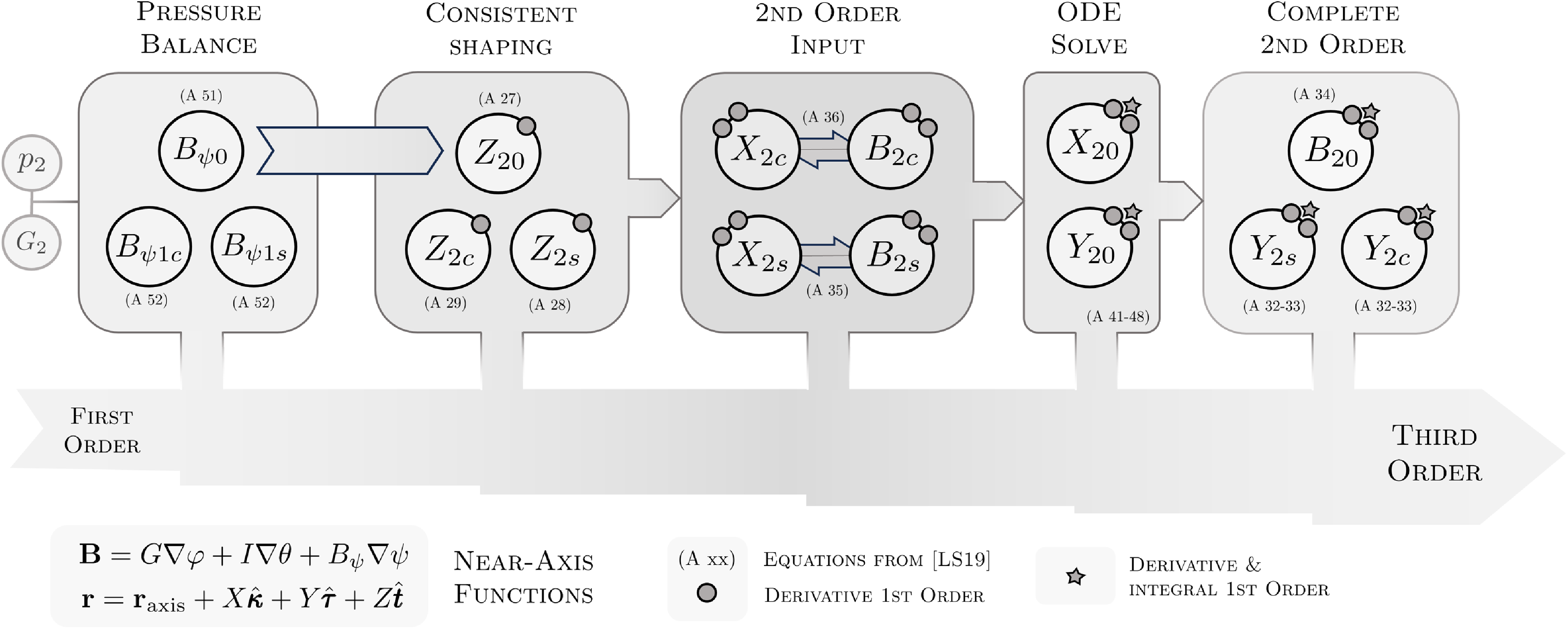
is summarised in a schematic way in figure 1, which we shall follow closely in the description that follows.
Inverse-coordinate near-axis construction to first order. Diagram depicting the key elements in the near-axis description of an equilibrium to first order, and the sequential order (left to right) in which to proceed. The construction starts with a shape for the magnetic axis and the magnetic field strength along it, both of which are given as inputs. To construct the neighbouring flux surfaces one must then provide the leading-order variation of the normal shaping $X_1$
, which directly relates to the field
$X_1$
, which directly relates to the field $B_1$
(this can go both ways). With that, one may then solve a differential equation on an auxiliary function
$B_1$
(this can go both ways). With that, one may then solve a differential equation on an auxiliary function $\sigma$
, which is all that is needed to complete the flux surface description through
$\sigma$
, which is all that is needed to complete the flux surface description through $Y_1$
. The encircled functions are the functions and parameters involved in the near-axis description, with the label (A xx) denoting the equations from Landreman & Sengupta (Reference Landreman and Sengupta2019) needed to find them.
$Y_1$
. The encircled functions are the functions and parameters involved in the near-axis description, with the label (A xx) denoting the equations from Landreman & Sengupta (Reference Landreman and Sengupta2019) needed to find them.
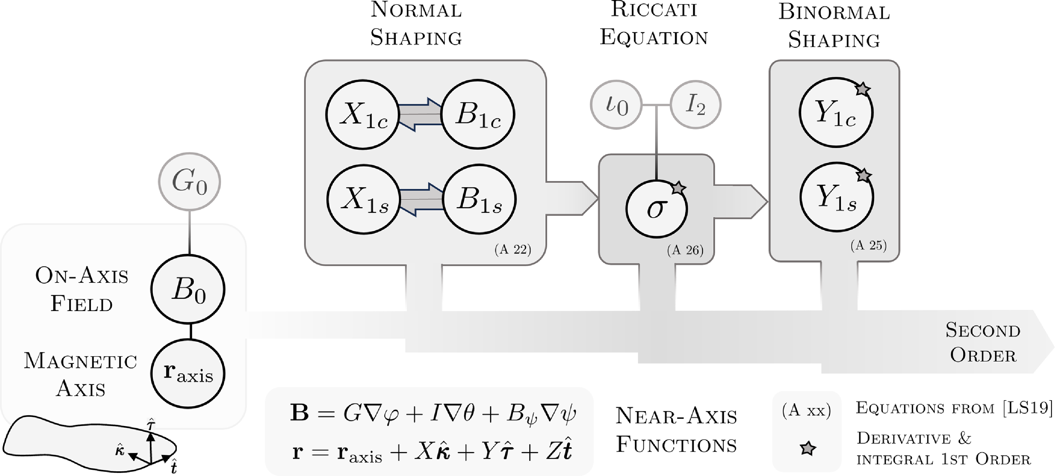
We already started (leftmost part of figure 1) the near-axis construction by the choice of an appropriate magnetic axis shape and the magnetic field strength on it. Naturally, when moving to $O(r)$
the field gains a finite flux surface build around the axis. Because of the analyticity constraint on the functions
$O(r)$
the field gains a finite flux surface build around the axis. Because of the analyticity constraint on the functions $X$
and
$X$
and $Y$
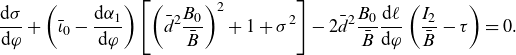
of (2.2), these surfaces must be elliptical in the FS frame. There is a certain amount of freedom available (although limited) in the problem to choose how to shape this elliptical surface (see figure 1). In particular, we must provide the function
$Y$
of (2.2), these surfaces must be elliptical in the FS frame. There is a certain amount of freedom available (although limited) in the problem to choose how to shape this elliptical surface (see figure 1). In particular, we must provide the function $X_1$
which specifies the distance along the normal from the flux surface to the axis as a function of
$X_1$
which specifies the distance along the normal from the flux surface to the axis as a function of $\chi$
and
$\chi$
and $\varphi$
. It is convenient to define it in terms of two
$\varphi$
. It is convenient to define it in terms of two $\phi$
-periodic functions (Garren & Boozer, Reference Garren and Boozer1991
Reference Garren and Boozerb
; Plunk et al. Reference Plunk, Landreman and Helander2019)
$\phi$
-periodic functions (Garren & Boozer, Reference Garren and Boozer1991
Reference Garren and Boozerb
; Plunk et al. Reference Plunk, Landreman and Helander2019) $\bar {d}(\varphi )\gt 0$
and
$\bar {d}(\varphi )\gt 0$
and $\alpha _1(\varphi )$
, such thatFootnote 2
$\alpha _1(\varphi )$
, such thatFootnote 2
 \begin{align} X_1=\bar {d}\cos \left (\chi -\alpha _1\right ). \\[-24pt] \nonumber \end{align}
The shaping $X_1$
is of particular physical significance: bringing the surface closer (further) to (from) the axis will (with a fixed gradient of
$X_1$
is of particular physical significance: bringing the surface closer (further) to (from) the axis will (with a fixed gradient of $B$
, from
$B$
, from $\nabla _\perp (B^2/2)=B^2\boldsymbol {\kappa }$
) lead to a larger (lower) magnetic field strength on the surface. Thus, the shaping brings in a direct control of the on-surface variation of
$\nabla _\perp (B^2/2)=B^2\boldsymbol {\kappa }$
) lead to a larger (lower) magnetic field strength on the surface. Thus, the shaping brings in a direct control of the on-surface variation of $|\mathbf {B}|$
. Within the context of the near axis, this formally translates to
$|\mathbf {B}|$
. Within the context of the near axis, this formally translates to $B_1=\kappa B_0X_1$
((A22) of LS). Note that this formulation is different from the standard one, where the magnetic field magnitude is provided as a control input to the problem (Garren & Boozer, Reference Garren and Boozer1991
Reference Garren and Boozera
; Landreman & Sengupta Reference Landreman and Sengupta2019; Rodríguez et al. Reference Rodríguez and Mackenbach2023; Landreman Reference Landreman2022). We need to do so because of the presence of ‘insensitive’ straight sections in which
$B_1=\kappa B_0X_1$
((A22) of LS). Note that this formulation is different from the standard one, where the magnetic field magnitude is provided as a control input to the problem (Garren & Boozer, Reference Garren and Boozer1991
Reference Garren and Boozera
; Landreman & Sengupta Reference Landreman and Sengupta2019; Rodríguez et al. Reference Rodríguez and Mackenbach2023; Landreman Reference Landreman2022). We need to do so because of the presence of ‘insensitive’ straight sections in which $B_1$
has an intrinsic form (in particular,
$B_1$
has an intrinsic form (in particular, $B_1=0$
wherever
$B_1=0$
wherever $\kappa =0$
). A similar observation will appear at higher orders.
$\kappa =0$
). A similar observation will appear at higher orders.
Specifying the distance from the surface to the axis along the normal only constitutes one part in the description of the shape of flux surfaces. To complete it, we must know the behaviour along the binormal as well. Finding that $Y_1$
constitutes the last steps of the first-order near-axis construction (see figure 1). To find it, we must remember that we are describing a flux surface, and thus any cross-section of the surface must be thread by a constant toroidal flux. This means that as the field strength changes in
$Y_1$
constitutes the last steps of the first-order near-axis construction (see figure 1). To find it, we must remember that we are describing a flux surface, and thus any cross-section of the surface must be thread by a constant toroidal flux. This means that as the field strength changes in $\varphi$
, so must the cross-sectional area, so that
$\varphi$
, so must the cross-sectional area, so that $X_1Y_1\sim 1/B_0$
. This justifies the condition
$X_1Y_1\sim 1/B_0$
. This justifies the condition $\bar {d}\gt 0$
, as flux surfaces would become infinitely elongated in the event of
$\bar {d}\gt 0$
, as flux surfaces would become infinitely elongated in the event of $\bar {d}$
ever vanishing. The exact relation between
$\bar {d}$
ever vanishing. The exact relation between $X_1$
and
$X_1$
and $Y_1$
is, however, not so simple, because besides the conservation of flux, one must make sure that the resulting surface is consistent with the solenoidal magnetic field that lives on it. The consequence of this careful balance is a strong relation between the shaping of the elliptic flux surfaces (including both the elongation and the rotation), the shape of the axis and the rotational transform,
$Y_1$
is, however, not so simple, because besides the conservation of flux, one must make sure that the resulting surface is consistent with the solenoidal magnetic field that lives on it. The consequence of this careful balance is a strong relation between the shaping of the elliptic flux surfaces (including both the elongation and the rotation), the shape of the axis and the rotational transform, $\iota _0$
.
$\iota _0$
.
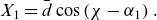
At a formal level, this careful balancing act reduces to the solution of a first-order nonlinear Riccati ( (Polyanin & Zaitsev Reference Polyanin and Zaitsev2017), § 1.4) differential equation ((A26) in LS) on a periodic auxiliary function $\sigma (\varphi )$
(taken in the stellarator symmetric case to satisfy
$\sigma (\varphi )$
(taken in the stellarator symmetric case to satisfy $\sigma (0)=0$
) and the rotational transform on axis,
$\sigma (0)=0$
) and the rotational transform on axis, $\iota _0$
,
$\iota _0$
,
 \begin{align} \frac {\mathrm {d}\sigma }{\mathrm {d}\varphi }+\left (\bar {\iota }_0-\frac {\mathrm {d}\alpha _1}{\mathrm {d}\varphi }\right )\left [\left (\bar {d}^2\frac { B_0}{\bar {B}}\right )^2+1+\sigma ^2\right ]-2\bar {d}^2\frac { B_0}{\bar {B}}\frac {\mathrm {d}\ell }{\mathrm {d}\varphi }\left (\frac {I_2}{\bar {B}}-\tau \right )=0. \end{align}
The rotational transform, here $\bar {\iota }_0=\iota _0-M$
, is a scalar parameter that must be chosen to guarantee periodicity of
$\bar {\iota }_0=\iota _0-M$
, is a scalar parameter that must be chosen to guarantee periodicity of $\sigma$
depending on the toroidal current
$\sigma$
depending on the toroidal current $I_2$
assumed (often set to zero) (Landreman & Sengupta Reference Landreman and Sengupta2018).Footnote 3 This equation has been explored in detail by other authors (Landreman, Sengupta & Plunk Reference Landreman, Sengupta and Plunk2019; Rodríguez et al. Reference Rodríguez and Mackenbach2023) and
$I_2$
assumed (often set to zero) (Landreman & Sengupta Reference Landreman and Sengupta2018).Footnote 3 This equation has been explored in detail by other authors (Landreman, Sengupta & Plunk Reference Landreman, Sengupta and Plunk2019; Rodríguez et al. Reference Rodríguez and Mackenbach2023) and $\sigma$
given a geometric interpretation of (roughly) signifying the rotation of the ellipses respect to the FS frame (Camacho Mata et al. Reference Camacho Mata, Plunk and Jorge2022; Rodríguez Reference Rodríguez2023). Once the
$\sigma$
given a geometric interpretation of (roughly) signifying the rotation of the ellipses respect to the FS frame (Camacho Mata et al. Reference Camacho Mata, Plunk and Jorge2022; Rodríguez Reference Rodríguez2023). Once the $\sigma$
-equation is solved,
$\sigma$
-equation is solved, $Y_1$
can be directly found ((A25) in LS),
$Y_1$
can be directly found ((A25) in LS),
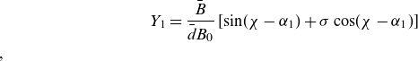 \begin{align} Y_1=\frac {\bar {B}}{\bar {d}B_0}\left [\sin\! (\chi -\alpha _1)+\sigma \cos\! (\chi -\alpha _1)\right ] \end{align},
and the first-order construction is completed.
2.4. Second-order near-axis construction
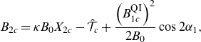
Much of the second-order construction can be understood as a natural continuation to the first order, where similar physics govern the way to proceed. There is, however, as indicated in figure 2, one significant difference: for the first time in the construction, the description of the field involves the pressure gradient, $p_2$
, directly. Sufficiently close to the axis, the magnetic field is force-free, which is why
$p_2$
, directly. Sufficiently close to the axis, the magnetic field is force-free, which is why $p$
was not involved at first order. The fulfilment of pressure balance is guaranteed by accommodating the magnetic field component
$p$
was not involved at first order. The fulfilment of pressure balance is guaranteed by accommodating the magnetic field component $B_\psi =\mathbf {B}\cdot \mathbf {e}_\psi$
(Boozer Reference Boozer1981). Formally, this involves the solution of simple first-order ordinary differential equations (ODEs) ((A51)–(A52) in LS), which may be done straightforwardly using periodic, vanishing endpoint boundary conditions. In addition, to balance a finite pressure gradient it is necessary to have a finite net current gradient. A formal statement of that is that
$B_\psi =\mathbf {B}\cdot \mathbf {e}_\psi$
(Boozer Reference Boozer1981). Formally, this involves the solution of simple first-order ordinary differential equations (ODEs) ((A51)–(A52) in LS), which may be done straightforwardly using periodic, vanishing endpoint boundary conditions. In addition, to balance a finite pressure gradient it is necessary to have a finite net current gradient. A formal statement of that is that $G_2+\iota _0 I_2$
(related to the radial variation of the net poloidal and toroidal currents), can be found algebraically at this point in the construction ((A50) in LS). Thus, there is one free constant in the second-order construction, with either
$G_2+\iota _0 I_2$
(related to the radial variation of the net poloidal and toroidal currents), can be found algebraically at this point in the construction ((A50) in LS). Thus, there is one free constant in the second-order construction, with either $G_2$
being determined by
$G_2$
being determined by $p_2$
or vice versa.
$p_2$
or vice versa.
Inverse-coordinate near-axis construction at second order. Diagram representing the key elements in the typical second-order near-axis equilibrium construction (left to right) to be taken as continuation of figure 1. The construction at second order starts by introducing the pressure gradient, $p_2$
, explicitly, which
$p_2$
, explicitly, which $B_\psi$
and the current
$B_\psi$
and the current $G_2$
must balance. The
$G_2$
must balance. The $Z_2$
shaping is then uniquely determined to remain consistent. Providing the
$Z_2$
shaping is then uniquely determined to remain consistent. Providing the $\theta$
-dependent shaping of
$\theta$
-dependent shaping of $X_2$
as input (or the, for poloidal
$X_2$
as input (or the, for poloidal $|\mathbf {B}|$
fields less convenient, alternative
$|\mathbf {B}|$
fields less convenient, alternative $B_2$
), the rest of the construction is uniquely determined, much like at first order. First one solves two coupled ODEs for the rigid displacement of flux surfaces (i.e. for
$B_2$
), the rest of the construction is uniquely determined, much like at first order. First one solves two coupled ODEs for the rigid displacement of flux surfaces (i.e. for $X_{20}$
and
$X_{20}$
and $Y_{20}$
), to finally complete the magnetic field and flux surface shaping in the binormal direction. The encircled functions are the key elements needed to describe the field, with the label (A xx) denoting the equations from Landreman & Sengupta (Reference Landreman and Sengupta2019) needed to find these quantities. The small circles on the edge of the functions denote that a derivative of lower-order quantities is required to compute the function. The star, in turn, denotes that the function is a solution of an ODE with a derivative of lower-order quantities in its inhomogeneous term.
$Y_{20}$
), to finally complete the magnetic field and flux surface shaping in the binormal direction. The encircled functions are the key elements needed to describe the field, with the label (A xx) denoting the equations from Landreman & Sengupta (Reference Landreman and Sengupta2019) needed to find these quantities. The small circles on the edge of the functions denote that a derivative of lower-order quantities is required to compute the function. The star, in turn, denotes that the function is a solution of an ODE with a derivative of lower-order quantities in its inhomogeneous term.
Once pressure is included in the problem, we solve for $Z_2$
(see figure 2). Formally, finding
$Z_2$
(see figure 2). Formally, finding $Z_2$
only involves operations of near-axis quantities already known, including their toroidal derivatives (see (A 27–29) in LS). This component describes the non-planar shape of cross-sections of constant
$Z_2$
only involves operations of near-axis quantities already known, including their toroidal derivatives (see (A 27–29) in LS). This component describes the non-planar shape of cross-sections of constant $\varphi$
. In that sense, it describes how the Boozer coordinate
$\varphi$
. In that sense, it describes how the Boozer coordinate $\varphi$
changes in the neighbourhood of the magnetic axis for it to remain consistent with the near-axis magnetic field.
$\varphi$
changes in the neighbourhood of the magnetic axis for it to remain consistent with the near-axis magnetic field.
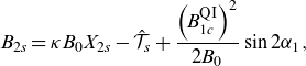
With the toroidal coordinate resolved, we now meet a step analogous to that with $X_1$
shaping at first order (see figure 2). We have the freedom to impose some shaping along the normal to the axis at second order. In particular, the second harmonic components
$X_1$
shaping at first order (see figure 2). We have the freedom to impose some shaping along the normal to the axis at second order. In particular, the second harmonic components $X_{2s}$
and
$X_{2s}$
and $X_{2c}$
, which affect directly the triangularity and up-down symmetry of the cross-sections (Rodríguez Reference Rodríguez2022, Reference Rodríguez2023). As it occurred at first order, the choice of this distance will, through the curvature, directly affect the corresponding harmonics of the second-order magnetic field strength
$X_{2c}$
, which affect directly the triangularity and up-down symmetry of the cross-sections (Rodríguez Reference Rodríguez2022, Reference Rodríguez2023). As it occurred at first order, the choice of this distance will, through the curvature, directly affect the corresponding harmonics of the second-order magnetic field strength $B_2$
((A 35–36) in LS),
$B_2$
((A 35–36) in LS),
 \begin{align} B_{2c} = \kappa B_0X_{2c}-\hat {\mathcal {T}}_c+\frac {\left(B_{1c}^{\mathrm {QI}} \right)^2}{2B_0}\cos 2\alpha _1, \\[-24pt] \nonumber \end{align}
 \begin{align} B_{2s}=\kappa B_0X_{2s}-\hat {\mathcal {T}}_s+\frac {\left(B_{1c}^{\mathrm {QI}} \right)^2}{2B_0}\sin 2\alpha _1, \\[6pt] \nonumber \end{align}
where $\hat {\mathcal {T}}_c$
and
$\hat {\mathcal {T}}_c$
and $\hat {\mathcal {T}}_s$
are known functions of first-order quantities (see appendix D), and
$\hat {\mathcal {T}}_s$
are known functions of first-order quantities (see appendix D), and $B_{1c}^{\mathrm {QI}}=B_0 \bar {d}\kappa$
. As it occurred at first order, at the straight sections of the field, the second-order shaping has no effect on the behaviour of the field (this favours, once again, the choice of
$B_{1c}^{\mathrm {QI}}=B_0 \bar {d}\kappa$
. As it occurred at first order, at the straight sections of the field, the second-order shaping has no effect on the behaviour of the field (this favours, once again, the choice of $X_2$
harmonics (
$X_2$
harmonics ( $X_{2c}$
and
$X_{2c}$
and $X_{2s}$
) as inputs, as opposed to
$X_{2s}$
) as inputs, as opposed to $B_2$
ones). At those points, the field becomes solely determined by the first-order solution. Elsewhere, the first-order solution also has a direct effect (physically from the need to preserve divergencelessness and tangent fieldlines), but present a larger degree of freedom. The choice
$B_2$
ones). At those points, the field becomes solely determined by the first-order solution. Elsewhere, the first-order solution also has a direct effect (physically from the need to preserve divergencelessness and tangent fieldlines), but present a larger degree of freedom. The choice $X_{2c}=0=X_{2s}$
, which we will refer to as minimal shaping, makes that underlying structure manifest at second order.
$X_{2c}=0=X_{2s}$
, which we will refer to as minimal shaping, makes that underlying structure manifest at second order.
From general MHD equilibria, we know that physical effects such as the Shafranov shift should come about here, influenced by the pressure gradient but also, and to a large extent, by the self-consistent shaping of the field ((Wesson Reference Wesson2011), § 3.7). This naturally brings us to the next step in the second-order near-axis construction (see figure 2), which is to self-consistently solve for $X_{20}$
and
$X_{20}$
and $Y_{20}$
. These two elements are measures of Shafranov shift in the normal and binormal direction (i.e. the relative rigid displacement of flux surfaces with radius) (Landreman Reference Landreman2021; Rodríguez Reference Rodríguez2022, Reference Rodríguez2023). To find these functions consistently with the rest of pieces of the construction requires the solution of two linear coupled first-order ODEs on
$Y_{20}$
. These two elements are measures of Shafranov shift in the normal and binormal direction (i.e. the relative rigid displacement of flux surfaces with radius) (Landreman Reference Landreman2021; Rodríguez Reference Rodríguez2022, Reference Rodríguez2023). To find these functions consistently with the rest of pieces of the construction requires the solution of two linear coupled first-order ODEs on $\varphi$
. These may be solved numerically in a straightforward way ((A41)–(A48) in LS), the considerations for half-helicity fields requiring us to work with half-periodic functions. With that solution and the second-order shaping inputs, the construction of the surface at second order is completed algebraically finding
$\varphi$
. These may be solved numerically in a straightforward way ((A41)–(A48) in LS), the considerations for half-helicity fields requiring us to work with half-periodic functions. With that solution and the second-order shaping inputs, the construction of the surface at second order is completed algebraically finding $Y_{2s}$
and
$Y_{2s}$
and $Y_{2c}$
to preserve, as we learnt at first order, the constant flux assumption as well as the appropriate shaping of the field lines over them ((A32)–(A33) in LS).
$Y_{2c}$
to preserve, as we learnt at first order, the constant flux assumption as well as the appropriate shaping of the field lines over them ((A32)–(A33) in LS).
Finally, we must compute the total magnetic field strength on the surface, of which only the second harmonics had been directly found after providing the normal shaping of the flux surfaces. The missing component is $B_{20}$
, i.e. the average
$B_{20}$
, i.e. the average $\psi$
-derivative of
$\psi$
-derivative of $|\mathbf {B}|$
on the surface. Of course, we could not compute this before knowing the complete shaping of the surfaces, and that is why its evaluation comes at last. Its construction is algebraic ((A34) in LS), similar to (2.7a)–(2.7
b
). Despite coming last in our solution method, the element
$|\mathbf {B}|$
on the surface. Of course, we could not compute this before knowing the complete shaping of the surfaces, and that is why its evaluation comes at last. Its construction is algebraic ((A34) in LS), similar to (2.7a)–(2.7
b
). Despite coming last in our solution method, the element $B_{20}$
plays a key role in physics, for instance MHD stability (Landreman & Jorge Reference Landreman and Jorge2020; Rodríguez Reference Rodríguez2023) and particle precession (Rodríguez & Mackenbach, Reference Rodríguez and Mackenbach2023; Rodríguez et al. Reference Rodríguez, Helander and Goodman2024).
$B_{20}$
plays a key role in physics, for instance MHD stability (Landreman & Jorge Reference Landreman and Jorge2020; Rodríguez Reference Rodríguez2023) and particle precession (Rodríguez & Mackenbach, Reference Rodríguez and Mackenbach2023; Rodríguez et al. Reference Rodríguez, Helander and Goodman2024).
This concludes the essential elements of the near-axis equilibrium construction at second order, for a field with poloidally closed $|\mathbf {B}|$
contours. The above holds regardless of whether the axis is half or integer helicity, though the former case does have subtleties related to periodicity and continuity, as discussed in appendix B.1.
$|\mathbf {B}|$
contours. The above holds regardless of whether the axis is half or integer helicity, though the former case does have subtleties related to periodicity and continuity, as discussed in appendix B.1.
3. Quasi-isodynamicity to second order
So far, the construction of the field near the axis has focused on the basic structure of an equilibrium stellarator symmetric magnetic field with nested flux surfaces and poloidally closed contours of $|\mathbf {B}|$
. These properties are not sufficient to ensure that field is omnigeneous (Hall & McNamara Reference Hall and McNamara1975; Cary & Shasharina Reference Cary and Shasharina1997) in the neighbourhood of the axis, i.e. the net radial drift of trapped particles will generally be non-vanishing. To complete the description of the field near the axis we must impose additional conditions, which in practice place severe constraints on the magnetic field magnitude
$|\mathbf {B}|$
. These properties are not sufficient to ensure that field is omnigeneous (Hall & McNamara Reference Hall and McNamara1975; Cary & Shasharina Reference Cary and Shasharina1997) in the neighbourhood of the axis, i.e. the net radial drift of trapped particles will generally be non-vanishing. To complete the description of the field near the axis we must impose additional conditions, which in practice place severe constraints on the magnetic field magnitude $|\mathbf {B}|$
.
$|\mathbf {B}|$
.
In the presence of stellarator symmetry, for the cancellation of the radial drift to occur, $|\mathbf {B}|$
must satisfy a number of symmetry conditions. This set of conditions on near-axis functions was originally derived to first order in Plunk et al. (Reference Plunk, Landreman and Helander2019), using the so-called Cary–Shasharina construction (Cary & Shasharina Reference Cary and Shasharina1997). In a recent paper (Rodríguez & Plunk, Reference Rodríguez and Plunk2023), the necessary conditions for quasi-isodynamicity were extended to second order in the near-axis expansion employing a more physical construction. Here we do not prove these conditions again, but simply present them, focusing on their consequences when considered alongside equilibrium.
$|\mathbf {B}|$
must satisfy a number of symmetry conditions. This set of conditions on near-axis functions was originally derived to first order in Plunk et al. (Reference Plunk, Landreman and Helander2019), using the so-called Cary–Shasharina construction (Cary & Shasharina Reference Cary and Shasharina1997). In a recent paper (Rodríguez & Plunk, Reference Rodríguez and Plunk2023), the necessary conditions for quasi-isodynamicity were extended to second order in the near-axis expansion employing a more physical construction. Here we do not prove these conditions again, but simply present them, focusing on their consequences when considered alongside equilibrium.
Let us start by recalling that in a stellarator symmetric configuration we must choose the magnetic field on axis to respect stellarator symmetry $B_0(\varphi )=B_0({-}\varphi )$
. That is, the magnetic well along the field line is symmetric, where
$B_0(\varphi )=B_0({-}\varphi )$
. That is, the magnetic well along the field line is symmetric, where $\varphi =0$
(in the domain
$\varphi =0$
(in the domain $\varphi \in [-\pi /N,\pi /N)$
and
$\varphi \in [-\pi /N,\pi /N)$
and $N$
is the number of field periods) corresponds to the bottom of the well and we consider a single well per field period. It is convenient to define the
$N$
is the number of field periods) corresponds to the bottom of the well and we consider a single well per field period. It is convenient to define the $\varphi$
domain in this way, as it simplifies the QI conditions. Defining
$\varphi$
domain in this way, as it simplifies the QI conditions. Defining $\varphi =0$
at
$\varphi =0$
at $B_{{max},0}$
as we do in the numerical implementation (and § 4) only lead to the addition of constant terms.Footnote 4 In order for the radial drift (
$B_{{max},0}$
as we do in the numerical implementation (and § 4) only lead to the addition of constant terms.Footnote 4 In order for the radial drift ( $\mathbf {v}_d\cdot \nabla \psi \sim \partial _\theta B_1$
) on each side of this well to cancel each other exactly, we require (Plunk et al. Reference Plunk, Landreman and Helander2019; Rodríguez & Plunk, Reference Rodríguez and Plunk2023)
$\mathbf {v}_d\cdot \nabla \psi \sim \partial _\theta B_1$
) on each side of this well to cancel each other exactly, we require (Plunk et al. Reference Plunk, Landreman and Helander2019; Rodríguez & Plunk, Reference Rodríguez and Plunk2023)
 \begin{align} {d}(\varphi )=-{d}({-}\varphi ), \end{align}
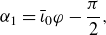 \begin{align} \alpha _1={\bar {\iota }_0}\varphi -\frac {\pi }{2}, \\[6pt] \nonumber \end{align}
where $d=\kappa \bar {d}$
and we have adopted the convention of
$d=\kappa \bar {d}$
and we have adopted the convention of $\alpha _1=-\pi /2$
at the bottom of the well.Footnote 5 Because by stellarator symmetry the curvature of the axis must have well defined parity about the bottom of the well,
$\alpha _1=-\pi /2$
at the bottom of the well.Footnote 5 Because by stellarator symmetry the curvature of the axis must have well defined parity about the bottom of the well, $\bar {d}$
must be even. From the first-order field construction it must also be non-zero,
$\bar {d}$
must be even. From the first-order field construction it must also be non-zero, $\bar {d}\gt 0$
. The signed curvature is then an odd function of
$\bar {d}\gt 0$
. The signed curvature is then an odd function of $\varphi$
at the bottom of the well, and thus it must have an odd zero of curvature there (as used in § 2.2). In addition to parity, the zero of curvature should be chosen to satisfy an additional condition to avoid breaking the poloidal topology of
$\varphi$
at the bottom of the well, and thus it must have an odd zero of curvature there (as used in § 2.2). In addition to parity, the zero of curvature should be chosen to satisfy an additional condition to avoid breaking the poloidal topology of $|\mathbf {B}|$
contours (i.e. bringing in puddles) at finite
$|\mathbf {B}|$
contours (i.e. bringing in puddles) at finite $r$
and thus violating omnigeneity (and in particular pseudosymmetry (Mikhailov et al. Reference Mikhailov, Shafranov, Subbotin, Isaev, Nührenberg, Zille and Cooper2002; Skovoroda Reference Skovoroda2005)) in the vicinity of field extrema. To achieve this, the order of the zero of curvature, call it
$r$
and thus violating omnigeneity (and in particular pseudosymmetry (Mikhailov et al. Reference Mikhailov, Shafranov, Subbotin, Isaev, Nührenberg, Zille and Cooper2002; Skovoroda Reference Skovoroda2005)) in the vicinity of field extrema. To achieve this, the order of the zero of curvature, call it $v$
, must be such that
$v$
, must be such that $d$
does not grow too strongly near the bottom of the
$d$
does not grow too strongly near the bottom of the $B_0$
well. This requires (see the discussion in Rodríguez & Plunk (Reference Rodríguez and Plunk2023))
$B_0$
well. This requires (see the discussion in Rodríguez & Plunk (Reference Rodríguez and Plunk2023)) $2v\geqslant u$
for
$2v\geqslant u$
for $B_0^{\prime}\sim \varphi ^{u-1}$
at the bottom of the well, and only equal when
$B_0^{\prime}\sim \varphi ^{u-1}$
at the bottom of the well, and only equal when $(u,v)=(2,1)$
. This very argument requires the critical points of
$(u,v)=(2,1)$
. This very argument requires the critical points of $B_0$
to match flattening points of the axis.Footnote 6
$B_0$
to match flattening points of the axis.Footnote 6
The other ingredient of QI at first order, the particular form of $\alpha _1$
, brings in an important issue. Quantities depending on
$\alpha _1$
, brings in an important issue. Quantities depending on $\alpha _1$
, including
$\alpha _1$
, including $B_1$
, are apparently not periodic (see (2.4)) if
$B_1$
, are apparently not periodic (see (2.4)) if $\alpha _1$
is not. In particular, unless
$\alpha _1$
is not. In particular, unless $\iota _0=M$
, the helicity of the axis, there will be a lack of periodicity across the edges of the domain (i.e. the top of the well). This is true even in the half-helicity case, as one must remember that
$\iota _0=M$
, the helicity of the axis, there will be a lack of periodicity across the edges of the domain (i.e. the top of the well). This is true even in the half-helicity case, as one must remember that $d$
is a half-periodic function. This limitation was recognised early in the construction of QI fields (Cary & Shasharina Reference Cary and Shasharina1997; Plunk et al. Reference Plunk, Landreman and Helander2019), and requires sacrificing omnigeneity in a finite region near the edges of the domain. These regions where a finite controlled deviation from QI is enacted through the function
$d$
is a half-periodic function. This limitation was recognised early in the construction of QI fields (Cary & Shasharina Reference Cary and Shasharina1997; Plunk et al. Reference Plunk, Landreman and Helander2019), and requires sacrificing omnigeneity in a finite region near the edges of the domain. These regions where a finite controlled deviation from QI is enacted through the function $\alpha _1$
(which as we saw in the equilibrium construction must be periodic) are called buffer regions (Plunk et al. Reference Plunk, Landreman and Helander2019; Camacho Mata et al. Reference Camacho Mata, Plunk and Jorge2022). There are multiple ways in which these buffer regions may be constructed, with various degrees of sophistication and smoothness associated with them. Defining the odd parity function
$\alpha _1$
(which as we saw in the equilibrium construction must be periodic) are called buffer regions (Plunk et al. Reference Plunk, Landreman and Helander2019; Camacho Mata et al. Reference Camacho Mata, Plunk and Jorge2022). There are multiple ways in which these buffer regions may be constructed, with various degrees of sophistication and smoothness associated with them. Defining the odd parity function $\tilde {\alpha }=\alpha _1+\pi /2$
(to preserve stellarator symmetry),
$\tilde {\alpha }=\alpha _1+\pi /2$
(to preserve stellarator symmetry), $\tilde {\alpha }$
must be constructed so that
$\tilde {\alpha }$
must be constructed so that $\tilde {\alpha }\approx \bar {\iota }\varphi$
in the central region and vanishes at the endpoints. The differences between different buffers arise in the details of how this is done. For the purpose of this paper, we shall consider two options. One we call standard, introduced in Camacho Mata et al. (Reference Camacho Mata, Plunk and Jorge2022), where a polynomial in
$\tilde {\alpha }\approx \bar {\iota }\varphi$
in the central region and vanishes at the endpoints. The differences between different buffers arise in the details of how this is done. For the purpose of this paper, we shall consider two options. One we call standard, introduced in Camacho Mata et al. (Reference Camacho Mata, Plunk and Jorge2022), where a polynomial in $\varphi$
is used to make
$\varphi$
is used to make $\tilde {\alpha }$
match
$\tilde {\alpha }$
match $2k+1$
derivatives with the ideal QI function at the bottom of the well, where
$2k+1$
derivatives with the ideal QI function at the bottom of the well, where $k\gt 0\in \mathbb {N}$
parametrises the family of buffers. Despite its simplicity, this choice has the potential issue presented by its non-smooth behaviour at the tops of the well, which, leads to discontinuous behaviour at second order in the construction. We present a smooth alternative, which we refer to as the smooth buffer, that is
$k\gt 0\in \mathbb {N}$
parametrises the family of buffers. Despite its simplicity, this choice has the potential issue presented by its non-smooth behaviour at the tops of the well, which, leads to discontinuous behaviour at second order in the construction. We present a smooth alternative, which we refer to as the smooth buffer, that is $C^\infty$
. In this case,
$C^\infty$
. In this case, $\tilde {\alpha }$
is written as a finite Fourier sine series, with its first
$\tilde {\alpha }$
is written as a finite Fourier sine series, with its first $2k+1$
derivatives matching those of the ideal QI scenario at the bottom of the well. The details of this and other constructions are presented in appendix B.2, alongside the issues of continuity and smoothness. Typical values of the parameter
$2k+1$
derivatives matching those of the ideal QI scenario at the bottom of the well. The details of this and other constructions are presented in appendix B.2, alongside the issues of continuity and smoothness. Typical values of the parameter $k$
correspond to
$k$
correspond to $k=5$
(roughly analogous to the
$k=5$
(roughly analogous to the $k=3$
choice for the standard construction, see table 3 in appendix B.2).
$k=3$
choice for the standard construction, see table 3 in appendix B.2).
Acknowledging and controlling the breaking of omnigeneity at first order through the use of buffers, we may construct physical fields that are approximately QI to first order. In the central region of the well the quality of omnigeneity is particularly high, and thus it is reasonable to ask about satisfying omnigeneity to next order there. Partial omnigeneity may be interpreted as the condition of no net radial drift for a part of the trapped particle population. For simplicity in the treatment, let us for now assume that the field is exactly QI at first order (see a more realistic treatment that takes the finite deviations into account in appendix C), and define
 \begin{align} B_2=B_{20}(\varphi )+B_{2c}(\varphi )\cos 2\chi +B_{2s}(\varphi )\sin 2\chi . \end{align}
A second-order QI field must then satisfy ((3.2a–c), Rodríguez & Plunk, Reference Rodríguez and Plunk2023)
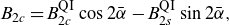 \begin{align} B_{2c}=B_{2c}^{\mathrm {QI}}\cos 2\bar {\alpha }-B_{2s}^{\mathrm {QI}}\sin 2\bar {\alpha }, \\[-6pt] \nonumber \end{align}
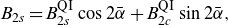 \begin{align} B_{2s}=B_{2s}^{\mathrm {QI}}\cos 2\bar {\alpha }+B_{2c}^{\mathrm {QI}}\sin 2\bar {\alpha }, \\[9pt] \nonumber \end{align}
where $\bar {\alpha }=\bar {\iota }_0\varphi -\pi /2$
is the ideal QI form of
$\bar {\alpha }=\bar {\iota }_0\varphi -\pi /2$
is the ideal QI form of $\alpha _1$
, and
$\alpha _1$
, and
 \begin{gather} B_{20}(\varphi )=B_{20}({-}\varphi ), \\[-24pt] \nonumber \end{gather}
 \begin{gather} B_{2s}^{\mathrm {QI}}(\varphi )=-B_{2s}^{\mathrm {QI}}({-}\varphi ),\\[-24pt] \nonumber \end{gather}
 \begin{gather} B_{2c}^{\mathrm {QI}}(\varphi )=\frac {1}{4}\left (\frac {B_0^2 d^2}{B_0^{\prime}}\right )^{\prime}, \\[-6pt] \nonumber \end{gather}
where primes denote derivatives in $\varphi$
. The first two conditions, (3.5a)–(3.5
b
), are statements of stellarator symmetry, and may be easily satisfied if we guarantee that everything in the problem has this symmetry. A straightforward analysis of the terms in (2.7a)–(2.7b) shows that the terms coming from first order have the right symmetry (see appendix D), and that the symmetry at second order is respected so long as one chooses
$\varphi$
. The first two conditions, (3.5a)–(3.5
b
), are statements of stellarator symmetry, and may be easily satisfied if we guarantee that everything in the problem has this symmetry. A straightforward analysis of the terms in (2.7a)–(2.7b) shows that the terms coming from first order have the right symmetry (see appendix D), and that the symmetry at second order is respected so long as one chooses $X_{2c}$
(
$X_{2c}$
( $X_{2s}$
) as odd (even) functions about the minimum of the well.
$X_{2s}$
) as odd (even) functions about the minimum of the well.
The third condition, (3.5c), is a more interesting one, as in this case $B_{2c}^{\mathrm {QI}}$
becomes fully determined by lower-order quantities. We now consider how to apply it to the relevant equilibrium equations, (2.7). For this comparison between QI and equilibrium, it is convenient to rewrite (2.7) in terms of
$B_{2c}^{\mathrm {QI}}$
becomes fully determined by lower-order quantities. We now consider how to apply it to the relevant equilibrium equations, (2.7). For this comparison between QI and equilibrium, it is convenient to rewrite (2.7) in terms of $B_{2c}^{\mathrm {QI}}$
, etc., by taking linear combinations as follows:
$B_{2c}^{\mathrm {QI}}$
, etc., by taking linear combinations as follows:
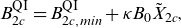 \begin{align} B_{2c}^{\mathrm {QI}}&=B_{2c,{min}}^{\mathrm {QI}}+\kappa B_0\tilde {X}_{2c}, \\[-6pt] \nonumber \end{align}
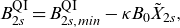 \begin{align} B_{2s}^{\mathrm {QI}}&=B_{2s,{min}}^{\mathrm {QI}}-\kappa B_0\tilde {X}_{2s}, \\[6pt] \nonumber \end{align}
where,
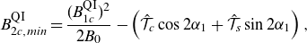 \begin{align} B_{2c,{min}}^{\mathrm {QI}}&=\frac {(B_{1c}^{\mathrm {QI}})^2}{2B_0}-\left (\hat {\mathcal {T}}_c\cos 2\alpha _1+\hat {\mathcal {T}}_s\sin 2\alpha _1\right ), \\[-6pt] \nonumber \end{align}
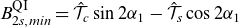 \begin{align} B_{2s,{min}}^{\mathrm {QI}}&=\hat {\mathcal {T}}_c\sin 2\alpha _1-\hat {\mathcal {T}}_s\cos 2\alpha _1 \\[6pt] \nonumber \end{align}
and $\tilde {X}_{2c}=X_{2c}\cos {2\alpha _1}+{X}_{2s}\sin {2\alpha _1}$
and
$\tilde {X}_{2c}=X_{2c}\cos {2\alpha _1}+{X}_{2s}\sin {2\alpha _1}$
and $\tilde {X}_{2s}={X}_{2c}\sin {2\alpha _1}-X_{2s}\cos {2\alpha _1}$
.
$\tilde {X}_{2s}={X}_{2c}\sin {2\alpha _1}-X_{2s}\cos {2\alpha _1}$
.
A straightforward attempt to impose omnigenity would be to simply substitute (3.5c) into (3.6a), yielding an algebraic equation for the free shaping function $\tilde {X}_{2c}$
. As hinted previously, however, the zeros of curvature complicate this, and a number of constraints at those points must be satisfied by the first order solution, depending of the order of those zeros, to ensure that shaping function
$\tilde {X}_{2c}$
. As hinted previously, however, the zeros of curvature complicate this, and a number of constraints at those points must be satisfied by the first order solution, depending of the order of those zeros, to ensure that shaping function $\tilde {X}_{2c}$
is non-singular.
$\tilde {X}_{2c}$
is non-singular.
To interpret what is happening, the omnigenity constraint imposed by (3.5c) can be thought of as ‘repairing’ defects in omnigeneity that are induced by the first-order solution. This requires specially shaping the second-order solution, but at locations where the axis straightens, such shaping is incapable of repairing the defects in omnigenity. One must do so by reaching back to first order, which boils down to satisfying additional pointwise constraints on the first-order solution. Namely,
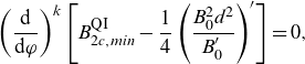 \begin{align} \left (\frac {\mathrm {d}}{\mathrm {d}\varphi }\right )^k\left [B_{2c,{min}}^{\mathrm {QI}}-\frac {1}{4}\left (\frac {B_0^2 d^2}{B_0^{\prime}}\right )^{\prime}\right ]=0, \end{align}
where $0\leqslant k\lt v$
. In short, looking at second order provides additional insight on the choices made at first order. A similar situation applies for
$0\leqslant k\lt v$
. In short, looking at second order provides additional insight on the choices made at first order. A similar situation applies for $B_{20}$
, the average radial derivative of
$B_{20}$
, the average radial derivative of $B$
(see the work in Rodríguez et al. (Reference Rodríguez, Helander and Goodman2024) for a discussion of it).
$B$
(see the work in Rodríguez et al. (Reference Rodríguez, Helander and Goodman2024) for a discussion of it).
Let us try to understand the contents of this condition by considering the leading order ( $k=0$
) implications of the constraint at the point of minimum
$k=0$
) implications of the constraint at the point of minimum $B_0$
. In the scenario of satisfying QI exactly at first order, we must satisfy at
$B_0$
. In the scenario of satisfying QI exactly at first order, we must satisfy at $\varphi =0$
,
$\varphi =0$
,
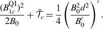 \begin{align} \frac {(B_{1c}^{\mathrm {QI}})^2}{2B_0}+\hat {\mathcal {T}}_c=\frac {1}{4}\left (\frac {B_0^2 d^2}{B_0^{\prime}}\right )^{\prime} .\end{align}
A local expansion in $\varphi$
(assuming the right-hand side to vanish)Footnote 7 yields
$\varphi$
(assuming the right-hand side to vanish)Footnote 7 yields
 \begin{align} \underbrace {\frac {\bar {d}^{\prime\prime}}{\bar {d}}\left (1+\frac {1}{e^2}\right )}_{\mathrm {Stretching}}+\underbrace {\frac {B_0^{\prime\prime}}{B_0}}_{\mathrm {Breathing}}+\underbrace {\left (\frac {\tau G_0}{B_0}\right )^2\left (1+\frac {3}{e^2}\right )}_{\mathrm {Rotation}}-\underbrace {\frac {4}{e^2}\left (\frac {G_0}{B_0}\right )^2\frac {I_2}{\bar {B}}\tau }_{\mathrm {Extra\ twist}}=0, \end{align}
where $e=\bar {B}/\bar {d}^2B_0$
is the elongation of the elliptic cross-section along the binormal at the bottom of the well and primes denote derivatives in
$e=\bar {B}/\bar {d}^2B_0$
is the elongation of the elliptic cross-section along the binormal at the bottom of the well and primes denote derivatives in $\varphi$
. This balance shows a physical competition between different elements that shape the resulting magnetic field lines. Stretching (variations in elongation) and breathing (variations in the cross-sectional area) of flux surfaces, alongside their rotation and twist shape field lines, and thus must collaborate to shape
$\varphi$
. This balance shows a physical competition between different elements that shape the resulting magnetic field lines. Stretching (variations in elongation) and breathing (variations in the cross-sectional area) of flux surfaces, alongside their rotation and twist shape field lines, and thus must collaborate to shape $B$
in a particular way so as to be omnigeneous. In the important stellarator-like scenario of minimal toroidal current, it follows from the above that it is necessary for
$B$
in a particular way so as to be omnigeneous. In the important stellarator-like scenario of minimal toroidal current, it follows from the above that it is necessary for $\bar {d}^{\prime\prime}/\bar {d}\lt 0$
, meaning that the cross-section will tend to become increasingly elongated (in the binormal direction) away from the bottom of the well. The larger the rotation and variation of
$\bar {d}^{\prime\prime}/\bar {d}\lt 0$
, meaning that the cross-section will tend to become increasingly elongated (in the binormal direction) away from the bottom of the well. The larger the rotation and variation of $B$
, the larger this stretching of flux surfaces needs to be.
$B$
, the larger this stretching of flux surfaces needs to be.
An additional $v-1$
constraints (where
$v-1$
constraints (where $v$
is the order of the zero of curvature) similar to (3.10) can be obtained by taking additional derivatives of (3.9) and matching functions order by order, as shown in (3.8). Once all such local requirements are satisfied, and this ‘straight’ mirror-like section of the field is left (sufficiently far from flattening points), one may obtain a well-behaved function
$v$
is the order of the zero of curvature) similar to (3.10) can be obtained by taking additional derivatives of (3.9) and matching functions order by order, as shown in (3.8). Once all such local requirements are satisfied, and this ‘straight’ mirror-like section of the field is left (sufficiently far from flattening points), one may obtain a well-behaved function $\tilde {X}_{2c}$
to enforce the second-order omnigenity constraint. However, this leaves us with little control on the amount of shaping at second order, which generally proves to be excessive (see some details on this way of approaching the problem in appendix E). If the emphasis is placed on minimising this shaping, we then have what we call the minimal shaping approach.
$\tilde {X}_{2c}$
to enforce the second-order omnigenity constraint. However, this leaves us with little control on the amount of shaping at second order, which generally proves to be excessive (see some details on this way of approaching the problem in appendix E). If the emphasis is placed on minimising this shaping, we then have what we call the minimal shaping approach.
The idea is to look for the subset of first-order fields for which one is capable of satisfying the omnigeneity condition at higher order, i.e. QI setting $X_{2s}=0=X_{2c}$
. In that case, the lower-order near-axis construction is fully responsible for the extent to which the field is more or less omnigeneous at second order. In practice this means that we need to choose
$X_{2s}=0=X_{2c}$
. In that case, the lower-order near-axis construction is fully responsible for the extent to which the field is more or less omnigeneous at second order. In practice this means that we need to choose $B_0$
,
$B_0$
, $\bar {d}$
and the axis shape (as well as
$\bar {d}$
and the axis shape (as well as $\alpha _1$
) so as to satisfy (3.9) in
$\alpha _1$
) so as to satisfy (3.9) in $\varphi$
(now not just at
$\varphi$
(now not just at $\varphi =0$
).
$\varphi =0$
).
Although we have verbalised the problem in a rather straightforward way, the problem is generally a hard one to solve (given its nonlinearity). It is thus natural to treat this as an optimisation problem where zeroth- and first-order inputs are varied to seek minimisation of $f_{\mathrm {QI}}=\left (B_{2c,{min}}^{\mathrm {QI}}-B_{2c}^{\mathrm {QI}}\right )^2$
, where the latter is the ideal omnigeneous form in (3.5c). Optimisation of near-axis fields is not unfamiliar (Landreman Reference Landreman2022; Jorge et al. Reference Jorge, Plunk, Drevlak, Landreman, Lobsien, Camacho Mata and Helander2022; Rodríguez et al. Reference Rodríguez and Mackenbach2023; Camacho-Mata & Plunk Reference Camacho-Mata and Plunk2023), and known codes and techniques may be used to that end. Recalling the presence of a buffer region extending from the tops of the well, it is logical to confine the optimisation of
$f_{\mathrm {QI}}=\left (B_{2c,{min}}^{\mathrm {QI}}-B_{2c}^{\mathrm {QI}}\right )^2$
, where the latter is the ideal omnigeneous form in (3.5c). Optimisation of near-axis fields is not unfamiliar (Landreman Reference Landreman2022; Jorge et al. Reference Jorge, Plunk, Drevlak, Landreman, Lobsien, Camacho Mata and Helander2022; Rodríguez et al. Reference Rodríguez and Mackenbach2023; Camacho-Mata & Plunk Reference Camacho-Mata and Plunk2023), and known codes and techniques may be used to that end. Recalling the presence of a buffer region extending from the tops of the well, it is logical to confine the optimisation of $f_{\mathrm {QI}}$
only to values of
$f_{\mathrm {QI}}$
only to values of $\varphi$
where the deviation of
$\varphi$
where the deviation of $\alpha _1$
from its ideal QI value is small. This qualitative choice of a region of interest can be made more quantitative by comparing the implications of breaking omnigeneity at first order to breaking it at second order. Some of the details are presented in appendix C. The main takeaway is nevertheless that wherever
$\alpha _1$
from its ideal QI value is small. This qualitative choice of a region of interest can be made more quantitative by comparing the implications of breaking omnigeneity at first order to breaking it at second order. Some of the details are presented in appendix C. The main takeaway is nevertheless that wherever $\alpha _{\mathrm {buf}}$
is small, then the QI
$\alpha _{\mathrm {buf}}$
is small, then the QI $B_{2c}$
criterion will dominate the behaviour, and thus one should enforce the QI condition there. We present an example of an optimised field following this construction in the next section.
$B_{2c}$
criterion will dominate the behaviour, and thus one should enforce the QI condition there. We present an example of an optimised field following this construction in the next section.
4. Numerical benchmark of second-order constructions
Having described the near-axis construction in detail in the preceding sections, we now present a number of numerical examples of near-axis fields with poloidal contours of $|\mathbf {B}|$
through (and including) second order. We do so for a variety of different inputs and benchmark the resulting constructions against the well established global equilibrium code VMEC (Hirshman & Whitson Reference Hirshman and Whitson1983). In that regard, we mirror the procedure in Landreman & Sengupta (Reference Landreman and Sengupta2019), which carried similar benchmarking work in the context of quasisymmetric fields. The agreement between the global solutions and the near-axis description in the limit of large aspect ratio should be taken as evidence of both the correct implementation of the near-axis code and the correctness of the near-axis construction. This numerical check is necessary to set a solid foundation to the second-order treatment of QI fields, so that it may be leveraged in future applications and studies.
$|\mathbf {B}|$
through (and including) second order. We do so for a variety of different inputs and benchmark the resulting constructions against the well established global equilibrium code VMEC (Hirshman & Whitson Reference Hirshman and Whitson1983). In that regard, we mirror the procedure in Landreman & Sengupta (Reference Landreman and Sengupta2019), which carried similar benchmarking work in the context of quasisymmetric fields. The agreement between the global solutions and the near-axis description in the limit of large aspect ratio should be taken as evidence of both the correct implementation of the near-axis code and the correctness of the near-axis construction. This numerical check is necessary to set a solid foundation to the second-order treatment of QI fields, so that it may be leveraged in future applications and studies.
To perform this numerical benchmark, we first need to construct the near-axis fields. We use numerical considerations like those spelled out in Landreman & Sengupta (Reference Landreman and Sengupta2019) and implemented in pyQSC. In the context of QI fields this was originally implemented in pyQIC, used in Jorge et al. (Reference Jorge, Plunk, Drevlak, Landreman, Lobsien, Camacho Mata and Helander2022), which we have significantly extended to appropriately deal with the second order.Footnote 8 In particular, a careful treatment of smoothness, buffers and the difficulties posed by half-helicity axes have been incorporated (these are the subject of some of the theoretical discussions touched upon in the main text and detailed in appendices B.1 and B.2).
Once we are able to numerically construct a near-axis field, we then proceed to make a comparison with global equilibria. We do so by constructing flux surface boundaries at different finite radii using the near-axis (Landreman & Sengupta Reference Landreman and Sengupta2019) (including the necessary third order fixes), and using them as inputs to global equilibria of different aspect ratios in VMEC (Hirshman & Whitson Reference Hirshman and Whitson1983).Footnote 9 The field near the axis may then be compared between the near-axis and global fields. To that end, we compute the magnetic field magnitude in Boozer coordinates using BOOZXFORM (Sanchez et al. Reference Sanchez, Hirshman, Ware, Berry and Spong2000), and by fitting the radial profiles of the various harmonics, construct estimates of $B_{0,\rm {VMEC}}$
,
$B_{0,\rm {VMEC}}$
, $B_{1,\rm {VMEC}}$
and
$B_{1,\rm {VMEC}}$
and $B_{2,\rm {VMEC}}$
. A comparison of the latter to
$B_{2,\rm {VMEC}}$
. A comparison of the latter to $B_2$
from within the near-axis framework and its behaviour across different aspect ratios,
$B_2$
from within the near-axis framework and its behaviour across different aspect ratios, $A$
, can then be used as a measure of correctness of the solution. We define
$A$
, can then be used as a measure of correctness of the solution. We define
 \begin{align} \Delta B_{{rms}.x}=\sqrt {\frac {1}{2\pi }\int _0^{2\pi }\left (B_{x}-B_{x,\rm {VMEC}}\right )^2\mathrm {d}\varphi }, \end{align}
for $x=20,\ 2s,\ 2c$
.
$x=20,\ 2s,\ 2c$
.
At extremely large aspect ratios ( $A\gt 100$
), the equilibrium solver starts to struggle finding solutions with the desired levels of accuracy, which hinders the comparison at such high values. The trend with
$A\gt 100$
), the equilibrium solver starts to struggle finding solutions with the desired levels of accuracy, which hinders the comparison at such high values. The trend with $A$
can nevertheless be used to judge the level of agreement between the asymptotic description and the full solution.
$A$
can nevertheless be used to judge the level of agreement between the asymptotic description and the full solution.
4.1. Minimally shaped vacuum configuration
Let us start our benchmark by looking at a simple case which we take from the recent publication of Camacho Mata et al. (Reference Camacho Mata, Plunk and Jorge2022). We consider the $N=2$
field in that paper, which is approximately QI at first order with a standard buffer region with
$N=2$
field in that paper, which is approximately QI at first order with a standard buffer region with $k=2$
. The axis is defined to have an integer helicity with first-order zeroes of curvature, parametrised by
$k=2$
. The axis is defined to have an integer helicity with first-order zeroes of curvature, parametrised by
 \begin{align} R\,[\text {m}] &= 1-\frac {1}{17}\cos 2\phi, \\[-6pt] \nonumber \end{align}
 \begin{align} Z\,[\text {m}] &= \frac {0.8}{2.04}\sin 2\phi +\frac {0.01}{2.04}\sin 4\phi, \\[9pt] \nonumber \end{align}
where the form of $R$
guarantees the correct behaviour of flattening points (Rodríguez et al. Reference Rodríguez, Sengupta and Bhattacharjee2022; Camacho Mata et al. Reference Camacho Mata, Plunk and Jorge2022). The magnetic field on axis is simply described by
$R$
guarantees the correct behaviour of flattening points (Rodríguez et al. Reference Rodríguez, Sengupta and Bhattacharjee2022; Camacho Mata et al. Reference Camacho Mata, Plunk and Jorge2022). The magnetic field on axis is simply described by $B_0\,[\text {T}]=1+0.15\cos 2\varphi$
, and
$B_0\,[\text {T}]=1+0.15\cos 2\varphi$
, and $\bar {d}=0.73$
is assumed constant. We extend this field into second order following the minimal shaping assumption; that is,
$\bar {d}=0.73$
is assumed constant. We extend this field into second order following the minimal shaping assumption; that is, $X_{2c}=0=X_{2s}$
. For this choice, the second-order field is a mere extension of the first order, and investigating the properties of this second-order completion may be used in the future as a tool to investigate the properties and suitability of the first-order near-axis construction, all within the near axis framework.
$X_{2c}=0=X_{2s}$
. For this choice, the second-order field is a mere extension of the first order, and investigating the properties of this second-order completion may be used in the future as a tool to investigate the properties and suitability of the first-order near-axis construction, all within the near axis framework.
Global equilibrium construction from the second-order near-axis field in § 4.1. The figure presents the second-order near-axis construction based on the $N=2$
field of Camacho Mata et al. (Reference Camacho Mata, Plunk and Jorge2022) presented in § 4.1. (a) Cross-sections at constant cylindrical angle in a half-period and 3-D rendering at
$N=2$
field of Camacho Mata et al. (Reference Camacho Mata, Plunk and Jorge2022) presented in § 4.1. (a) Cross-sections at constant cylindrical angle in a half-period and 3-D rendering at $A=10$
. The dotted line traces the magnetic axis, with crosses representing the intersection with the cross-sections. (b) Root-mean-square difference in the second-order near-axis magnetic field between the ideal near-axis description and the finite aspect ratio global equilibrium construction with VMEC. A reference quadratic scaling
$A=10$
. The dotted line traces the magnetic axis, with crosses representing the intersection with the cross-sections. (b) Root-mean-square difference in the second-order near-axis magnetic field between the ideal near-axis description and the finite aspect ratio global equilibrium construction with VMEC. A reference quadratic scaling $\propto 1/A^2$
is given, from which the convergence of the error deviated at larger aspect ratios. (c) Explicit comparison between the different poloidal components of the second-order magnetic field magnitude from the global VMEC equilibrium at different aspect ratios, and the ideal near-axis value (black dotted line).
$\propto 1/A^2$
is given, from which the convergence of the error deviated at larger aspect ratios. (c) Explicit comparison between the different poloidal components of the second-order magnetic field magnitude from the global VMEC equilibrium at different aspect ratios, and the ideal near-axis value (black dotted line).
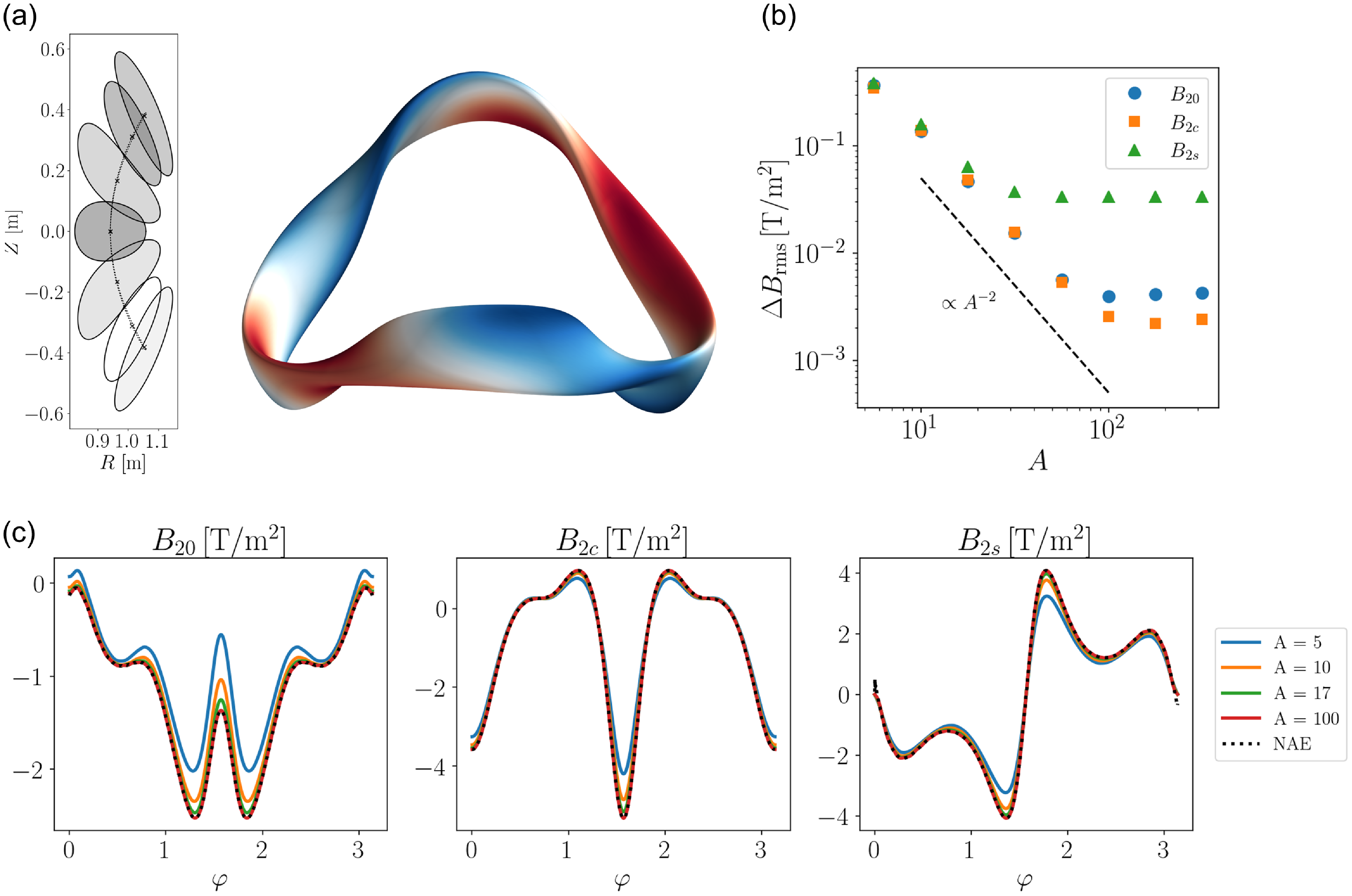
The construction of the near-axis field and the comparison with the global equilibrium is shown in figure 3. The top left plots show cross-sections and a flux surface of the configuration evaluated at $r\,[\text {m}]=0.1$
, which roughly corresponds to an aspect ratio of
$r\,[\text {m}]=0.1$
, which roughly corresponds to an aspect ratio of $A=1/r=10$
. The bottom plot shows a direct comparison between the different components of
$A=1/r=10$
. The bottom plot shows a direct comparison between the different components of $B_2$
as a function of
$B_2$
as a function of $\varphi$
for a number of aspect ratios, showing that as the aspect ratio
$\varphi$
for a number of aspect ratios, showing that as the aspect ratio $A$
is increased, the agreement becomes better. Even at as low an aspect ratio as
$A$
is increased, the agreement becomes better. Even at as low an aspect ratio as $A=5$
the second-order near-axis construction reproduces the behaviour of the equilibrium at least qualitatively. This points towards the significance and physical nature of second-order properties. The top right plot shows the level of agreement as a function of aspect ratio in a more quantitative fashion. It shows the root-mean-square difference between the VMEC and near-axis functions defined in (4.1). Although there is an initial improvement with increasing aspect ratio at small
$A=5$
the second-order near-axis construction reproduces the behaviour of the equilibrium at least qualitatively. This points towards the significance and physical nature of second-order properties. The top right plot shows the level of agreement as a function of aspect ratio in a more quantitative fashion. It shows the root-mean-square difference between the VMEC and near-axis functions defined in (4.1). Although there is an initial improvement with increasing aspect ratio at small $A$
, this seems to saturate quite rapidly (at approximately
$A$
, this seems to saturate quite rapidly (at approximately $A\sim 20$
). The reason behind this discrepancy can be traced to the behaviour of
$A\sim 20$
). The reason behind this discrepancy can be traced to the behaviour of $B_{2s}$
in figure 3(c). Near the endpoints of the domain, one can see that the function
$B_{2s}$
in figure 3(c). Near the endpoints of the domain, one can see that the function $B_{2s}$
from the near-axis construction is actually discontinuous. And of course, the global equilibrium solve cannot reproduce such unphysical features. Hence the saturation of the error at a level dictated by the size of the discontinuity.
$B_{2s}$
from the near-axis construction is actually discontinuous. And of course, the global equilibrium solve cannot reproduce such unphysical features. Hence the saturation of the error at a level dictated by the size of the discontinuity.
The origin of said discontinuity had already been discussed in the main text preceding this section: it is the lack of smoothness in the standard buffer. To show that this is responsible for the observed disagreement, we repeat the same numerical exercise, but this time using a smooth buffer with $k=5$
. The results are shown in figure 4, where the previous saturation of the error disappears.
$k=5$
. The results are shown in figure 4, where the previous saturation of the error disappears.
Comparison of second-order field of the equilibrium in figure 3 with smooth buffer regions. The figure presents the comparison of the second-order near-axis field for the same configuration as in figure 3 but for the difference in the analyticity of the construction near the field edges. (a) Root-mean-square difference in the second-order near-axis magnetic field between the ideal near-axis description and the finite aspect ratio global equilibrium construction with VMEC. A reference quadratic scaling $\propto 1/A^2$
is given, from which the convergence of the error deviated at larger aspect ratios. (c) Explicit comparison between the different poloidal components of the second-order magnetic field magnitude from the global VMEC equilibrium at different aspect ratios, and the ideal near-axis value (black dotted line). The agreement near the edge is better than that of figure 3.
$\propto 1/A^2$
is given, from which the convergence of the error deviated at larger aspect ratios. (c) Explicit comparison between the different poloidal components of the second-order magnetic field magnitude from the global VMEC equilibrium at different aspect ratios, and the ideal near-axis value (black dotted line). The agreement near the edge is better than that of figure 3.
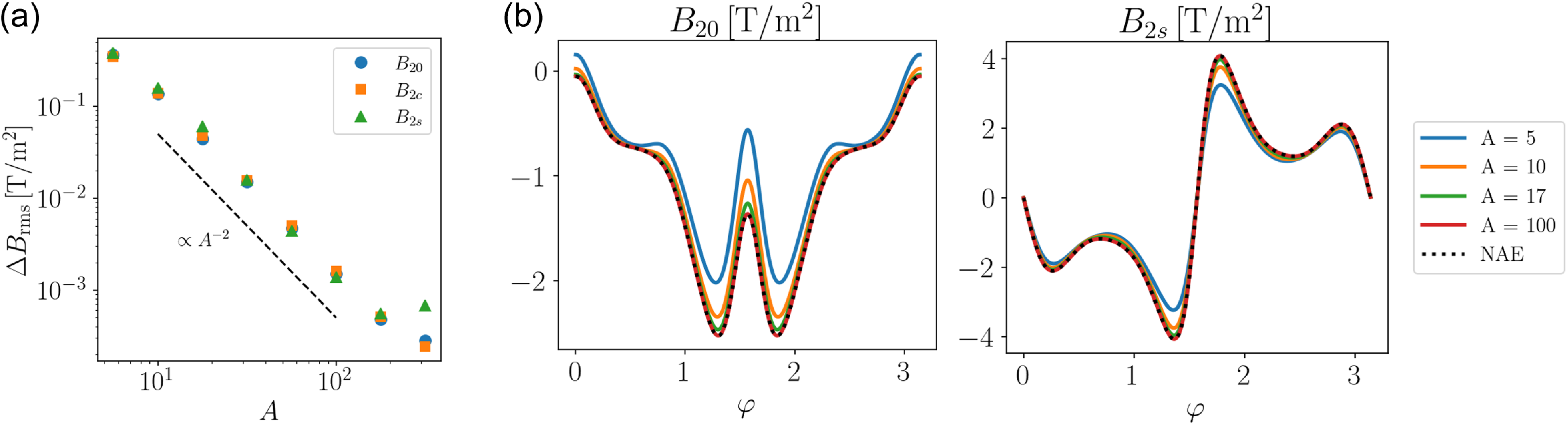
The disagreement between the near-axis and global equilibrium scales like $\sim 1/A^2$
(this is the difference in the second-order field
$\sim 1/A^2$
(this is the difference in the second-order field $B_2$
, and not
$B_2$
, and not $r^2B_2$
). This quadratic reduction of the error is expected from a construction that is accurate to second order, as the finite build of the near axis is (Landreman & Sengupta Reference Landreman and Sengupta2019). This requires the error to be at least
$r^2B_2$
). This quadratic reduction of the error is expected from a construction that is accurate to second order, as the finite build of the near axis is (Landreman & Sengupta Reference Landreman and Sengupta2019). This requires the error to be at least $1/A$
, but because of analyticity of the field near the magnetic axis, the
$1/A$
, but because of analyticity of the field near the magnetic axis, the $m=0,2$
harmonics only exhibit even powers and thus the scaling with
$m=0,2$
harmonics only exhibit even powers and thus the scaling with $1/A^2$
. This behaviour is observed over a wide range of aspect ratios. At the highest values of aspect ratio (in figure 4,
$1/A^2$
. This behaviour is observed over a wide range of aspect ratios. At the highest values of aspect ratio (in figure 4, $A=316$
) there appears to be some level of discrepancy as VMEC struggles to converge (note, however, the high demands we are placing on the code, as we require the field to be correct to approximately 1 part in
$A=316$
) there appears to be some level of discrepancy as VMEC struggles to converge (note, however, the high demands we are placing on the code, as we require the field to be correct to approximately 1 part in $10^8$
or more).
$10^8$
or more).
With this first example we show that: (i) the near-axis construction to second order for QI fields works; (ii) that the non-smooth constructions cannot be faithfully reproduced by global physical equilibria; but (iii) that their qualitative aspects can.
4.2.
Shaped, finite plasma- $\beta$
configuration
$\beta$
configuration

We now consider a more involved example that includes finite plasma $\beta$
and non-zero explicit second-order shaping. In this case, we base the construction off the
$\beta$
and non-zero explicit second-order shaping. In this case, we base the construction off the $N=3$
in Camacho Mata et al. (Reference Camacho Mata, Plunk and Jorge2022), with a smooth buffer region. The axis is defined approximately by
$N=3$
in Camacho Mata et al. (Reference Camacho Mata, Plunk and Jorge2022), with a smooth buffer region. The axis is defined approximately by
 \begin{align} R [\text {m}] & = 1+ 0.09075485\cos 3\phi -0.02058279 \cos 6\phi -0.01106766\cos 9\phi \nonumber\\ & \qquad -0.001644390e \cos 12\phi, \end{align}
 \begin{align} Z [\text {m}] & = 0.36 \sin 3\phi + 0.02\sin 6\phi + 0.01\sin 9\phi, \end{align}
which when implemented numerically one should carefully check to satisfy the vanishing curvature condition at the stellarator symmetric points. The magnetic strength on axis is $B_0\,[\text {T}]=1+0.25\cos 3\varphi$
, and
$B_0\,[\text {T}]=1+0.25\cos 3\varphi$
, and $\bar {d}=0.73$
once again. In this case we choose some arbitrary non-zero values for
$\bar {d}=0.73$
once again. In this case we choose some arbitrary non-zero values for $X_{2c}[\text {m}^{-1}]=0.1\sin 3\varphi -0.6\sin 6\varphi +0.1\sin 9\varphi$
and
$X_{2c}[\text {m}^{-1}]=0.1\sin 3\varphi -0.6\sin 6\varphi +0.1\sin 9\varphi$
and $X_{2s}[\text {m}^{-1}]=0.1-0.1\cos 6\varphi +0.6\cos 9\varphi$
. Finally, we put a finite toroidal current
$X_{2s}[\text {m}^{-1}]=0.1-0.1\cos 6\varphi +0.6\cos 9\varphi$
. Finally, we put a finite toroidal current $I_2\,[\text {T/m}] = -0.9$
and pressure gradient
$I_2\,[\text {T/m}] = -0.9$
and pressure gradient $p_2\,[\text {Pa/m}^2]=-6\times 10^5$
. The resulting field and comparison with VMEC is presented in figure 5. Once again, the quadratic scaling of the error shows agreement between the near-axis construction and the global equilibrium solve. Note that this time the equilibrium is significantly more shaped than in the case of § 4.1, in part as a consequence of the larger number of field periods (and thus larger toroidal derivatives) but also the explicit shaping introduced at second order. This increased complexity is apparent in the comparison of the different components of
$p_2\,[\text {Pa/m}^2]=-6\times 10^5$
. The resulting field and comparison with VMEC is presented in figure 5. Once again, the quadratic scaling of the error shows agreement between the near-axis construction and the global equilibrium solve. Note that this time the equilibrium is significantly more shaped than in the case of § 4.1, in part as a consequence of the larger number of field periods (and thus larger toroidal derivatives) but also the explicit shaping introduced at second order. This increased complexity is apparent in the comparison of the different components of $B_2$
, but also on the scaling of the error
$B_2$
, but also on the scaling of the error $\Delta B_{{rms}}$
itself, as the deviations from the ideal scaling occur at lower aspect ratios. This case is an example of one of the struggles in the design of near-axis QI fields, which is to avoid this extreme shaping.
$\Delta B_{{rms}}$
itself, as the deviations from the ideal scaling occur at lower aspect ratios. This case is an example of one of the struggles in the design of near-axis QI fields, which is to avoid this extreme shaping.
Global equilibrium construction from the second-order near-axis field in § 4.2. The figure presents the second-order near-axis construction based on Camacho Mata et al. (Reference Camacho Mata, Plunk and Jorge2022) presented in § 4.1 including finite $\beta$
, toroidal current and additional second-order shaping. (a) Cross-sections at constant cylindrical angle in a half-period and 3-D rendering at
$\beta$
, toroidal current and additional second-order shaping. (a) Cross-sections at constant cylindrical angle in a half-period and 3-D rendering at $A=10$
. The dotted line traces the magnetic axis, with crosses representing the intersection with the cross-sections. (b) Root-mean-square difference in the second-order near-axis magnetic field between the ideal near-axis description and the finite aspect ratio global equilibrium construction with VMEC. A reference quadratic scaling
$A=10$
. The dotted line traces the magnetic axis, with crosses representing the intersection with the cross-sections. (b) Root-mean-square difference in the second-order near-axis magnetic field between the ideal near-axis description and the finite aspect ratio global equilibrium construction with VMEC. A reference quadratic scaling $\propto 1/A^2$
is given, from which the convergence of the error deviated at larger aspect ratios. (c) Explicit comparison between the different poloidal components of the second-order magnetic field magnitude from the global VMEC equilibrium at different aspect ratios, and the ideal near-axis value (black dotted line).
$\propto 1/A^2$
is given, from which the convergence of the error deviated at larger aspect ratios. (c) Explicit comparison between the different poloidal components of the second-order magnetic field magnitude from the global VMEC equilibrium at different aspect ratios, and the ideal near-axis value (black dotted line).

4.3. Half-helicity case
The same systematic construction can be followed for the special QI class of fields with half-helicity axes. We construct an $N=3$
half-helicity field with a smooth
$N=3$
half-helicity field with a smooth $k=5$
buffer. When dealing with half-helicity axes, and especially when high control is required on the curvature and torsion, as is indeed needed in order to control the extreme shaping that is the tendency of QI fields, it is convenient to define the axis by directly parametrising the curvature and the torsion. In that case, one needs to reconstruct the axis by integrating FS equations, (2.3). The well-known drawback of doing so is that curvature and torsion must be chosen carefully to guarantee closure of the axis, which must be achieved numerically to a sufficiently high degree of accuracy. Failing to do so will lead to discontinuities (or lack of smoothness in the best of cases) in the near-axis construction of flux surfaces, and thus will lead to an unphysical field.Footnote 10 Taking this into account, we consider in this case,
$k=5$
buffer. When dealing with half-helicity axes, and especially when high control is required on the curvature and torsion, as is indeed needed in order to control the extreme shaping that is the tendency of QI fields, it is convenient to define the axis by directly parametrising the curvature and the torsion. In that case, one needs to reconstruct the axis by integrating FS equations, (2.3). The well-known drawback of doing so is that curvature and torsion must be chosen carefully to guarantee closure of the axis, which must be achieved numerically to a sufficiently high degree of accuracy. Failing to do so will lead to discontinuities (or lack of smoothness in the best of cases) in the near-axis construction of flux surfaces, and thus will lead to an unphysical field.Footnote 10 Taking this into account, we consider in this case,
 \begin{gather} \kappa [\text {m}^{-1}]=-\frac {8.0725268}{2}\left [1+\cos \left (6\pi \frac {\ell }{L}\right )\right ]\sin \left (3\pi \frac {\ell }{L}\right )\sin \left (6\pi \frac {\ell }{L}\right ), \\[-24pt] \nonumber \end{gather}
 \begin{gather} \tau [\text {m}^{-1}]= 1.34174997-0.133333\cos \left (6\pi \frac {\ell }{L}\right ), \\[6pt] \nonumber \end{gather}
and $L [\text {m}]= 2\pi$
, which gives a third-order zero at the bottom of the well and second order at the top. The magnetic field
$L [\text {m}]= 2\pi$
, which gives a third-order zero at the bottom of the well and second order at the top. The magnetic field $B_0$
and the shaping
$B_0$
and the shaping $\bar {d}$
are not presented explicitly in the text, but can be found in the repository associated with this paper, as they have been chosen carefully to limit the amount of elongation and shaping of the construction. The steps informing the choice of inputs and the use of the FS approach will be detailed in a future publication. We complete the inputs to the near-axis construction by choosing
$\bar {d}$
are not presented explicitly in the text, but can be found in the repository associated with this paper, as they have been chosen carefully to limit the amount of elongation and shaping of the construction. The steps informing the choice of inputs and the use of the FS approach will be detailed in a future publication. We complete the inputs to the near-axis construction by choosing $X_{2c}=0=X_{2s}$
.
$X_{2c}=0=X_{2s}$
.
Global equilibrium construction from the second-order near-axis field in § 4.3. The figure presents a second-order near-axis construction for a half-helicity, three period field. (a) Cross-sections at constant cylindrical angle in a half-period and 3-D rendering at $A=10$
. The dotted line traces the magnetic axis, with crosses representing the intersection with the cross-sections. (b) Root-mean-square difference in the second-order near-axis magnetic field between the ideal near-axis description and the finite aspect ratio global equilibrium construction with VMEC. A reference quadratic scaling
$A=10$
. The dotted line traces the magnetic axis, with crosses representing the intersection with the cross-sections. (b) Root-mean-square difference in the second-order near-axis magnetic field between the ideal near-axis description and the finite aspect ratio global equilibrium construction with VMEC. A reference quadratic scaling $\propto 1/A^2$
is given, from which the convergence of the error deviated at larger aspect ratios. The VMEC solver struggles at larger aspect ratios. (c) Explicit comparison between the different poloidal components of the second-order magnetic field magnitude from the global VMEC equilibrium at different aspect ratios, and the ideal near-axis value (black dotted line).
$\propto 1/A^2$
is given, from which the convergence of the error deviated at larger aspect ratios. The VMEC solver struggles at larger aspect ratios. (c) Explicit comparison between the different poloidal components of the second-order magnetic field magnitude from the global VMEC equilibrium at different aspect ratios, and the ideal near-axis value (black dotted line).
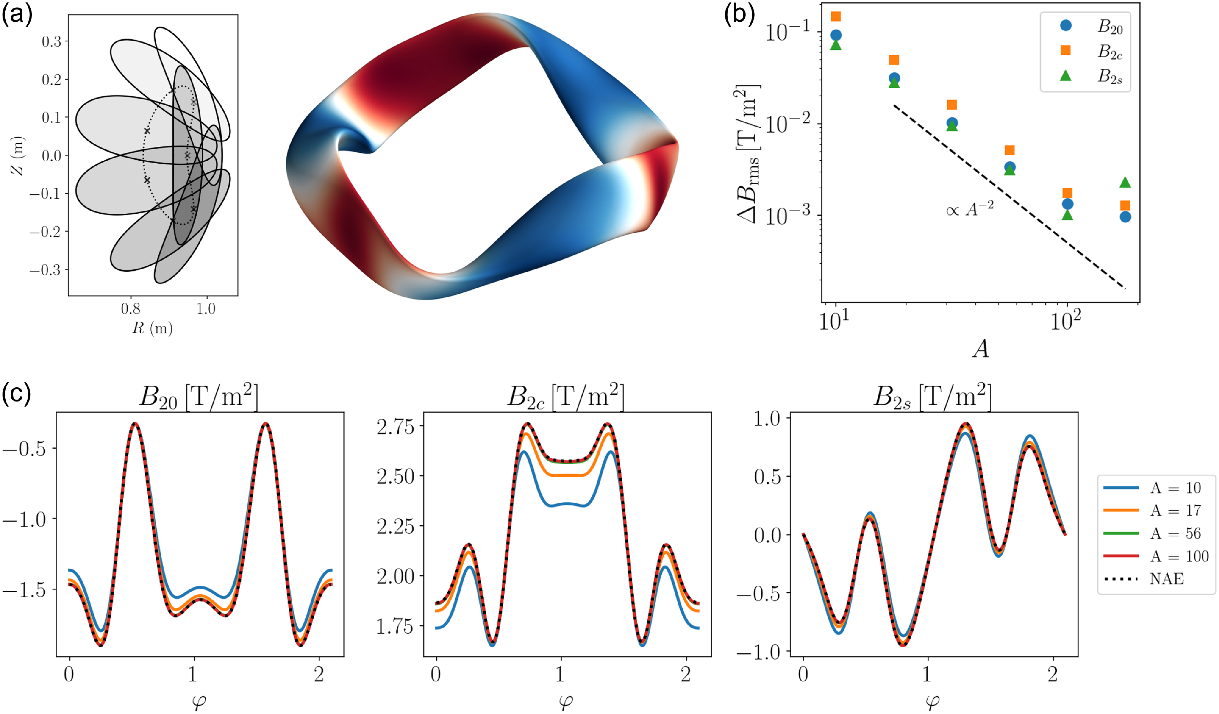
The results of the comparison with VMEC are shown in figure 6, where we get the expected agreement. This shows that the treatment of the half-helicity scenario (as discussed in § 2 and appendix B.1) and is indeed the correct one.
4.4. The QI optimised minimally shaped field
Finally, we present a field which has been optimised to be omnigeneous at second order near the bottom of the well following § 3. In this proof-of-principle exercise, we allowed the $Z$
harmonics as well as
$Z$
harmonics as well as $\bar {d}$
to vary as our degrees of freedom, and penalise deviations from omnigeneity at second order in the central 20 % of the domain. The starting point of the construction was the same as that of § 4.2, namely the
$\bar {d}$
to vary as our degrees of freedom, and penalise deviations from omnigeneity at second order in the central 20 % of the domain. The starting point of the construction was the same as that of § 4.2, namely the $N=3$
from Camacho Mata et al. (Reference Camacho Mata, Plunk and Jorge2022). The resulting
$N=3$
from Camacho Mata et al. (Reference Camacho Mata, Plunk and Jorge2022). The resulting $Z$
component of the axis,
$Z$
component of the axis,
 \begin{align} Z [\text {m}] \approx 0.397890 \sin 3\phi + 0.0244030\sin 6\phi + 0.00292413\sin 9\phi, \end{align}
and
 \begin{align} \bar {d} \approx 0.642233+0.000346819\cos 6\varphi +0.00114030\cos 9\varphi &+0.00366299\cos 12\varphi \nonumber \\ &-0.00230278\cos 15\varphi . \end{align}
Global equilibrium construction from the second-order near-axis field in § 4.4. The figure presents the second-order near-axis construction based on Camacho Mata et al. (Reference Camacho Mata, Plunk and Jorge2022) presented in § 4.4 that has been reshaped to satisfy the QI criterion at second order near $B_{{min}}$
. (a) Cross-sections at constant cylindrical angle in a half-period and 3-D rendering at
$B_{{min}}$
. (a) Cross-sections at constant cylindrical angle in a half-period and 3-D rendering at $A=10$
. The dotted line traces the magnetic axis, with crosses representing the intersection with the cross-sections. (b) Root-mean-square difference in the second-order near-axis magnetic field between the ideal near-axis description and the finite aspect ratio global equilibrium construction with VMEC. A reference quadratic scaling
$A=10$
. The dotted line traces the magnetic axis, with crosses representing the intersection with the cross-sections. (b) Root-mean-square difference in the second-order near-axis magnetic field between the ideal near-axis description and the finite aspect ratio global equilibrium construction with VMEC. A reference quadratic scaling $\propto 1/A^2$
is given, from which the convergence of the error deviated at larger aspect ratios. (c) Explicit comparison between the different poloidal components of the second-order magnetic field magnitude from the global VMEC equilibrium at different aspect ratios, and the ideal near-axis value (black dotted line). The shaded region indicates the
$\propto 1/A^2$
is given, from which the convergence of the error deviated at larger aspect ratios. (c) Explicit comparison between the different poloidal components of the second-order magnetic field magnitude from the global VMEC equilibrium at different aspect ratios, and the ideal near-axis value (black dotted line). The shaded region indicates the $\varphi$
range optimised for QI at second order.
$\varphi$
range optimised for QI at second order.
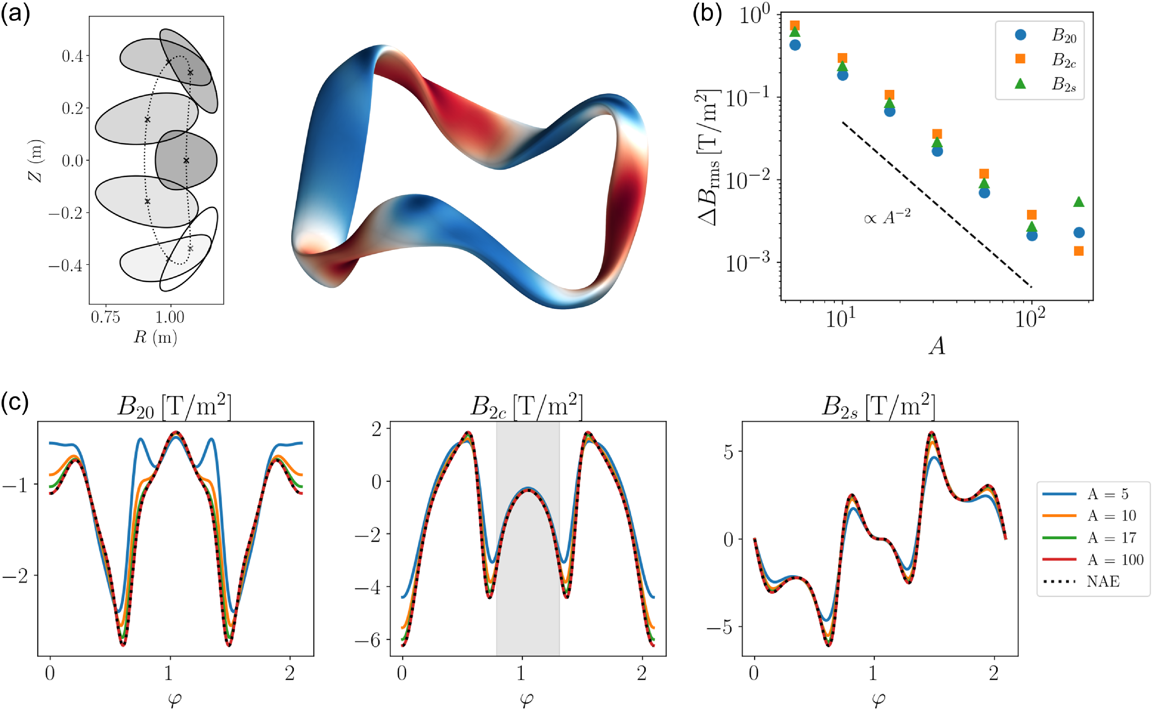
Once again, the comparison with VMEC shows agreement (see figure 7) over a range of aspect ratios, struggling to converge at very large aspect ratios, likely driven by the high degree of toroidal variation.
5. Conclusions
In this work we have described the practical and theoretical details that allow the solution of MHD equilibrium equations to second order in the near-axis expansion for the case of QI stellarators. For the first time, we are able to ‘directly construct’ configurations of this key class of stellarators to second order.
Our work builds on two previous works, Landreman & Sengupta (Reference Landreman and Sengupta2019) and Rodríguez & Plunk (Reference Rodríguez and Plunk2023), the first of which, although focusing on the class of quasisymmetric stellarators, established a general roadmap for constructing second-order stellarator equilibria, and the second of which described the necessary conditions to enforce the QI to this second order. To help make the discussion easier to follow, we provide a physical guide into the second-order theory, describing the solution process, inputs outputs and interdependencies; see in particular figures 1 and 2.
To fully extend second-order near-axis framework, it was necessary to establish appropriate forms of the inputs to the theory at both first and second order, with the latter being coupled to the former during the solution process. The case of half-helicity was found to be particularly subtle. This is also the case that tends to be found in integrated optimisation studies, so is particularly important to treat properly here. We established conditions to ensure continuity and smoothness of such solutions to the necessary order.
A key issue explored in this work is the degree to which the QI condition can be satisfied, in principle and in practice. At first order, it has been established that some violation is necessary for barely trapped particles (Plunk et al. Reference Plunk, Landreman and Helander2019), but here we present an approach to achieving higher-order QI that can make meaningful improvements on the first-order solution for deeply trapped particles. We show how the construction at first order directly impacts the behaviour at second order, especially near the field extrema. With that we learn that only special choices of these parameters and functions are consistent with a high degree of omnigeneity.
Finally, a thorough benchmarking was performed to verify the theoretical derivations and numerical implementation for the different topological classes of QI stellarators, and for both vacuum and finite-pressure solutions. The numerical examples show detailed asymptotic agreement with global equilibria solved with VMEC.
Near-axis theory is an important tool for tackling fundamental theoretical questions in stellarator optimisation, and has a number of practical applications such as initialising optimisation studies, and enabling the efficient exploration of optimisation space. These and other activities are greatly enhanced by completing the near axis, theory to second order, to incorporate key physics like stability, equilibrium shaping and effects related to plasma pressure such as the Shafaronov shift. Our results extend near-axis theory as a theoretical and practical tool for studying QI stellarators and can immediately benefit all activities that depend on it.
Acknowledgements
The authors would like to thank the help provided by J. Geiger, S. Lazerson and M. Cianciosa with VMEC, as well as fruitful discussion with M. Landreman and D. Panici.
Editor Peter Catto thanks the referees for their advice in evaluating this article.
Data availability
The data and scripts that support the findings of this study are openly available at the Zenodo repository with DOI/URL 10.5281/zenodo.13860071.
Declaration of interests
The authors report no conflict of interest.
Funding
E.R. was supported by a grant by Alexander-von-Humboldt-Stiftung, Bonn, Germany, through a postdoctoral research fellowship.
Appendix A. Theory of stellarator symmetric space curves with flattening points
Let us start this appendix by setting our object of study: a simple regular closed curve $\gamma :\ S^1\rightarrow \mathbb {R}^3$
. By simple we mean non-intersecting, and by regular that the curve is continuous and infinitely differentiable, parametrised by the length
$\gamma :\ S^1\rightarrow \mathbb {R}^3$
. By simple we mean non-intersecting, and by regular that the curve is continuous and infinitely differentiable, parametrised by the length $\ell$
along the curve. The curve length is defined to be
$\ell$
along the curve. The curve length is defined to be $L$
, which is the period of the parametrisation. Such a curve may be described by its
$L$
, which is the period of the parametrisation. Such a curve may be described by its $\mathbb {R}^3$
embedding
$\mathbb {R}^3$
embedding $\mathbf {r}_{{axis}}(\ell )$
.
$\mathbf {r}_{{axis}}(\ell )$
.
In order to introduce the standard notion of stellarator symmetry (Dewar & Hudson Reference Dewar and Hudson1998), it is convenient to frame the curve in a cylindrical coordinate system. In particular, we specialise for simplicity to curves that may be parametrised by the cylindrical angle $\phi$
in such a way that
$\phi$
in such a way that $\ell (\phi )$
is a bounded, strictly monotonically increasing function of
$\ell (\phi )$
is a bounded, strictly monotonically increasing function of $\phi$
with
$\phi$
with $\ell (0)=0$
and
$\ell (0)=0$
and $\ell (2\pi )=L$
. This guarantees a one-to-one between
$\ell (2\pi )=L$
. This guarantees a one-to-one between $\ell$
and
$\ell$
and $\phi$
, which we shall also take to be
$\phi$
, which we shall also take to be $C^\infty$
. The curve is therefore
$C^\infty$
. The curve is therefore $2\pi$
-periodic in
$2\pi$
-periodic in $\phi$
. This consideration rules out special curve shapes such as those whose projection onto the
$\phi$
. This consideration rules out special curve shapes such as those whose projection onto the $z=0$
plane do not correspond to the boundary of a star-shaped domain or curves with straight sections in the
$z=0$
plane do not correspond to the boundary of a star-shaped domain or curves with straight sections in the $z$
direction. With this, we write our embedded curve as
$z$
direction. With this, we write our embedded curve as
 \begin{align} \mathbf {r}_{{axis}}(\phi )=R(\phi )\hat {\boldsymbol{R}}(\phi )+Z(\phi )\hat {{\textit{z}}}, \end{align}
where $\{\hat {{\boldsymbol{R}}}(\phi ),\hat {\boldsymbol {\phi }}(\phi ), \hat { {\textit{z}}}\}$
represent the orthonormal basis of the cylindrical coordinates
$\{\hat {{\boldsymbol{R}}}(\phi ),\hat {\boldsymbol {\phi }}(\phi ), \hat { {\textit{z}}}\}$
represent the orthonormal basis of the cylindrical coordinates $\{R,\phi, z\}$
. We consider the functions
$\{R,\phi, z\}$
. We consider the functions $R$
and
$R$
and $Z$
to be
$Z$
to be $C^\infty$
and
$C^\infty$
and $2\pi$
-periodic in
$2\pi$
-periodic in $\phi$
, to provide a regular, smooth curve.
$\phi$
, to provide a regular, smooth curve.
We say a curve to be stellarator symmetric (Dewar & Hudson Reference Dewar and Hudson1998) about a point $\mathbf {r}_{{axis}}(\phi _0)$
if
$\mathbf {r}_{{axis}}(\phi _0)$
if $R(\phi _0+\hat {\phi })=R(\phi _0-\hat {\phi })$
and
$R(\phi _0+\hat {\phi })=R(\phi _0-\hat {\phi })$
and $Z(\phi _0+\hat {\phi })=-Z(\phi _0-\hat {\phi })$
. That is,
$Z(\phi _0+\hat {\phi })=-Z(\phi _0-\hat {\phi })$
. That is, $R$
is even and
$R$
is even and $Z$
is odd about stellarator-symmetric points. Note that by virtue of periodicity, stellarator symmetric points always come in pairs:
$Z$
is odd about stellarator-symmetric points. Note that by virtue of periodicity, stellarator symmetric points always come in pairs: $(\phi _0,\phi _0+\pi )$
for
$(\phi _0,\phi _0+\pi )$
for $0\leqslant \phi _0\lt \pi$
.
$0\leqslant \phi _0\lt \pi$
.
With our curve defined, we may try to construct the tangent to the curve, $ \hat {{\textit{t}}}$
. By definition,
$ \hat {{\textit{t}}}$
. By definition,
 \begin{align} \hat {{\textit{t}}}=\frac {\mathrm {d}\mathbf {r}_{{axis}}}{\mathrm {d}\ell }=\frac {1}{\ell ^{\prime}}\left [R^{\prime}\hat {\boldsymbol{R}}+R\hat {\boldsymbol {\phi }}+Z^{\prime}\hat {{\textit{z}}}\right ] \; : \; \begin{pmatrix} \mathrm {O} \\ \mathrm {E} \\ \mathrm {E} \end{pmatrix}_{\mathrm {cyl}}, \end{align}
where $\ell ^{\prime}=\sqrt {R^2+(R^{\prime})^2+(Z^{\prime})^2}\gt 0$
and primes denote derivatives with respect to
$\ell ^{\prime}=\sqrt {R^2+(R^{\prime})^2+(Z^{\prime})^2}\gt 0$
and primes denote derivatives with respect to $\phi$
(not
$\phi$
(not $\varphi$
as in the main text). The last part of the equality indicates the parity about the stellarator symmetric point that the three components of the vector (in the cylindrical basis) have following the properties of
$\varphi$
as in the main text). The last part of the equality indicates the parity about the stellarator symmetric point that the three components of the vector (in the cylindrical basis) have following the properties of $R$
and
$R$
and $Z$
, namely, even (E) and odd (O). This means that at stellarator symmetric points the curve must be orthogonal to
$Z$
, namely, even (E) and odd (O). This means that at stellarator symmetric points the curve must be orthogonal to $\hat {{\boldsymbol{R}}}$
.
$\hat {{\boldsymbol{R}}}$
.
To understand how this curve twists, we shall continue taking additional derivatives of the curve. Constructing
 \begin{align} \mathbf {r}_{{axis}}^{\prime\prime}=\left (R^{\prime\prime}-R\right )\hat {{\boldsymbol{R}}}+2R^{\prime}\hat {\boldsymbol {\phi }}+Z^{\prime\prime}\hat {{\textit{z}}}, \end{align}
we define the vector orthogonal to the curve,
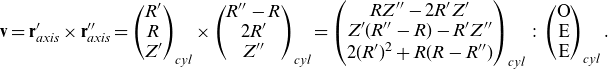 \begin{align} \mathbf {v}=\mathbf {r}_{{axis}}^{\prime}\times \mathbf {r}_{{axis}}^{\prime\prime}=\begin{pmatrix} R^{\prime} \\ R \\ Z^{\prime} \end{pmatrix}_{{cyl}}\times \begin{pmatrix} R^{\prime\prime}-R \\ 2R^{\prime} \\ Z^{\prime\prime} \end{pmatrix}_{{cyl}} =\begin{pmatrix} RZ^{\prime\prime}-2R^{\prime}Z^{\prime} \\ Z^{\prime}(R^{\prime\prime}-R)-R^{\prime}Z^{\prime\prime} \\ 2(R^{\prime})^2+R(R-R^{\prime\prime}) \end{pmatrix}_{ {cyl}} \; : \; \begin{pmatrix} \mathrm {O} \\ \mathrm {E} \\ \mathrm {E} \end{pmatrix}_{{cyl}}. \end{align}
This vector $\mathbf {v}$
has a very special interpretation in the context of space curves, as it is parallel to the conventional Frenet binormal vector (Mathews & Walker Reference Mathews and Walker1964; Animov Reference Animov2001), which we will denote
$\mathbf {v}$
has a very special interpretation in the context of space curves, as it is parallel to the conventional Frenet binormal vector (Mathews & Walker Reference Mathews and Walker1964; Animov Reference Animov2001), which we will denote $\hat {\boldsymbol {\tau }}_{\text {F}}=\mathbf {v}/|\mathbf {v}|$
. The binormal is uniquely defined then provided
$\hat {\boldsymbol {\tau }}_{\text {F}}=\mathbf {v}/|\mathbf {v}|$
. The binormal is uniquely defined then provided $\mathbf {r}_{{axis}}^{\prime}$
and
$\mathbf {r}_{{axis}}^{\prime}$
and $\mathbf {r}_{{axis}}^{\prime\prime}$
are linearly independent (and
$\mathbf {r}_{{axis}}^{\prime\prime}$
are linearly independent (and $\mathbf {r}_{{axis}}^{\prime\prime}$
is non-vanishing).
$\mathbf {r}_{{axis}}^{\prime\prime}$
is non-vanishing).
In addition to the above, the vector $\mathbf {v}$
can also be directly linked to the notion of curvature,
$\mathbf {v}$
can also be directly linked to the notion of curvature, $\kappa$
, defined as
$\kappa$
, defined as
 \begin{align} |\kappa |=\frac {1}{(\ell ^{\prime})^3}|\mathbf {v}|=\frac {1}{(\ell ^{\prime})^3}\sqrt {\left (v^R\right )^2+\left (v^\phi \right )^2+\left (v^z\right )^2}, \end{align}
where we have written the components of $\mathbf {v}$
explicitly.
$\mathbf {v}$
explicitly.
We call a point $\mathbf {r}_{{axis}}(\phi _0)$
at which
$\mathbf {r}_{{axis}}(\phi _0)$
at which $\kappa =0$
a flattening point. We characterise such points by a natural number
$\kappa =0$
a flattening point. We characterise such points by a natural number $\nu \in \mathbb {N}_{\gt 0}$
which we call the order of the flattening point or of the zero of curvature, defined as the order of the first non-vanishing
$\nu \in \mathbb {N}_{\gt 0}$
which we call the order of the flattening point or of the zero of curvature, defined as the order of the first non-vanishing $\phi$
derivative of the curvature
$\phi$
derivative of the curvature $\kappa$
. The properties of this point will determine the behaviour of the binormal in its neighbourhood.
$\kappa$
. The properties of this point will determine the behaviour of the binormal in its neighbourhood.
Let us now specialise to curves for which every point of stellarator symmetry is also a flattening point, as is required by omnigenity at first order. Because of the well-defined parity of the components of $\mathbf {v}$
, it is straightforward to see that the flattening point condition requires
$\mathbf {v}$
, it is straightforward to see that the flattening point condition requires $v^\phi (\phi _0)=0=v^z(\phi _0)$
(which are the even components). If the curvature were non-zero at
$v^\phi (\phi _0)=0=v^z(\phi _0)$
(which are the even components). If the curvature were non-zero at $\phi _0$
, then the binormal would be perpendicular to the radial direction, but this is not necessarily the case when
$\phi _0$
, then the binormal would be perpendicular to the radial direction, but this is not necessarily the case when $\kappa =0$
, because the leading components in the
$\kappa =0$
, because the leading components in the $\phi$
and
$\phi$
and $z$
directions also vanish. In fact, the orientation of the binormal in the neighbourhood of the point (and we say neighbourhood, because at the flattening point
$z$
directions also vanish. In fact, the orientation of the binormal in the neighbourhood of the point (and we say neighbourhood, because at the flattening point $\mathbf {v}=0$
) depends critically on which the order of the zero is. It is convenient to rewrite the order
$\mathbf {v}=0$
) depends critically on which the order of the zero is. It is convenient to rewrite the order $\nu$
for a stellarator symmetric flattening point as
$\nu$
for a stellarator symmetric flattening point as
 \begin{align} \nu =\min \left [ \{n\in \mathbb {N}^{{even}} \,:\, \partial _\phi ^n v^\phi \neq 0\ \mathrm {or}\ \partial _\phi ^n v^z \neq 0\} \cup \{n\in \mathbb {N}^{{odd}} \,:\, \partial _\phi ^n v^R \neq 0\}\right ], \end{align}
where parity of the various terms has been here leveraged. Depending on whether $\nu$
is even or odd, it is the odd or even parity components of
$\nu$
is even or odd, it is the odd or even parity components of $\mathbf {v}$
, respectively that will be first non-zero in the neighbourhood of the flattening point. This leading component defines the direction of
$\mathbf {v}$
, respectively that will be first non-zero in the neighbourhood of the flattening point. This leading component defines the direction of $\hat {\boldsymbol {\tau }}_{\text {F}}=\mathbf {v}/|\mathbf {v}|$
. If
$\hat {\boldsymbol {\tau }}_{\text {F}}=\mathbf {v}/|\mathbf {v}|$
. If $\nu \in \mathbb {N}^{\mathrm {even}}$
, the binormal is orthogonal to
$\nu \in \mathbb {N}^{\mathrm {even}}$
, the binormal is orthogonal to $\hat {{\boldsymbol {R}}}$
,
$\hat {{\boldsymbol {R}}}$
, $\hat {\boldsymbol {\tau }}_{\text {F}}\cdot \hat {{\boldsymbol{R}}}=0$
. Of course, as all the components of the vector
$\hat {\boldsymbol {\tau }}_{\text {F}}\cdot \hat {{\boldsymbol{R}}}=0$
. Of course, as all the components of the vector $\mathbf {v}$
are
$\mathbf {v}$
are $C^\infty$
, so will the Frenet frame across the said point. In the case of an odd order
$C^\infty$
, so will the Frenet frame across the said point. In the case of an odd order $\nu$
,
$\nu$
, $\hat {\boldsymbol {\tau }}_{\text {F}}$
becomes aligned with the radial direction
$\hat {\boldsymbol {\tau }}_{\text {F}}$
becomes aligned with the radial direction $\hat {{\boldsymbol{R}}}$
near the flattening point, and does actually undergoes a flip across it. This is the case because the dominant behaviour of
$\hat {{\boldsymbol{R}}}$
near the flattening point, and does actually undergoes a flip across it. This is the case because the dominant behaviour of $\mathbf {v}$
is odd in this scenario, and thus
$\mathbf {v}$
is odd in this scenario, and thus $\mathbf {v}/|\mathbf {v}|$
points in opposite directions. The Frenet frame is therefore discontinuous across odd flattening points.
$\mathbf {v}/|\mathbf {v}|$
points in opposite directions. The Frenet frame is therefore discontinuous across odd flattening points.
This discontinuity can be nevertheless reverted by redefining the binormal as part of the so-called signed frame (Plunk et al. Reference Plunk, Landreman and Helander2019), called also the $\beta$
frame by Carroll et al. (Reference Carroll, Köse and Sterling2013). In such a frame, the direction of the binormal is flipped across odd flattening points in such a way that it becomes continuous. The key insight is that this modified binormal can be shown to satisfy the FS equations, provided the curvature (and also the normal vector) are also signed. This flip makes the frame continuous across the flattening point, but it also makes it smooth. Throughout the text we denote the signed Frenet frame as
$\beta$
frame by Carroll et al. (Reference Carroll, Köse and Sterling2013). In such a frame, the direction of the binormal is flipped across odd flattening points in such a way that it becomes continuous. The key insight is that this modified binormal can be shown to satisfy the FS equations, provided the curvature (and also the normal vector) are also signed. This flip makes the frame continuous across the flattening point, but it also makes it smooth. Throughout the text we denote the signed Frenet frame as $(\hat {{\textit{t}}}, \hat {\boldsymbol {\kappa }},\hat {\boldsymbol {\tau }})$
, distinct from the conventional Frenet frame,
$(\hat {{\textit{t}}}, \hat {\boldsymbol {\kappa }},\hat {\boldsymbol {\tau }})$
, distinct from the conventional Frenet frame, $(\hat {{\textit{t}}}, \hat {\boldsymbol {\kappa }}_{\text {F}},\hat {\boldsymbol {\tau }}_{\text {F}})$
. Likewise we reserve the symbol
$(\hat {{\textit{t}}}, \hat {\boldsymbol {\kappa }}_{\text {F}},\hat {\boldsymbol {\tau }}_{\text {F}})$
. Likewise we reserve the symbol $\kappa$
to denote the signed curvature. Upon flipping the sign about an odd zero,
$\kappa$
to denote the signed curvature. Upon flipping the sign about an odd zero,
 \begin{align} \hat {\boldsymbol {\tau }}(\phi ) \; : \; \begin{pmatrix} \mathrm {E}^o \\ \mathrm {O}^o \\ \mathrm {O}^o \end{pmatrix}_{{cyl}}, \end{align}
where the superscript $^o$
indicates the odd order of the point. For an even flattening point, these components have the opposite parity.
$^o$
indicates the odd order of the point. For an even flattening point, these components have the opposite parity.
Now that we know how the binormal vector behaves, we can construct a complete picture of the signed FS frame, with the normal vector defined as
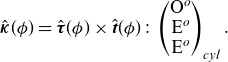 \begin{align} \hat {\boldsymbol {\kappa }}(\phi )=\hat {\boldsymbol {\tau }}(\phi ) \times \hat {{\textit{t}}}(\phi ) \; : \; \begin{pmatrix} \mathrm {O}^o \\ \mathrm {E}^o \\ \mathrm {E}^o \end{pmatrix}_{{cyl}}. \end{align}
Just to be clear, if the order of curvature is even, then the parity of the components of $\hat {\boldsymbol {\kappa }}$
and
$\hat {\boldsymbol {\kappa }}$
and $\hat {\boldsymbol {\tau }}$
are reversed.
$\hat {\boldsymbol {\tau }}$
are reversed.
There is an interesting question to be asked here about whether the signed frame is continuous or not globally. We have argued about these properties locally across a flattening point, but after going around the whole curve, the question remains of whether after all the flipping involved, the frame at $\phi =0$
is the same as
$\phi =0$
is the same as $\phi =2\pi$
. To that end, let us label each of the flattening points in our curve by an index
$\phi =2\pi$
. To that end, let us label each of the flattening points in our curve by an index $i\in \mathbb {N}\,:\, 0\leqslant i\lt n$
, where
$i\in \mathbb {N}\,:\, 0\leqslant i\lt n$
, where $n\in \mathbb {N}^{{even}}$
is the total number of points. To each point we assign an order of zeros
$n\in \mathbb {N}^{{even}}$
is the total number of points. To each point we assign an order of zeros $\nu _i$
. As we follow the axis, we define the total order of the curve as
$\nu _i$
. As we follow the axis, we define the total order of the curve as $\mathcal {V}=\sum _{i=0}^{n-1}\nu _i$
. The signed frame of a curve with an even order will be globally continuous. This is obviously true if all flattening points are even order; in case of an even number of odd such points, every time we cross one such point we gain a sign flip, and thus if an even number of these flips is to be counted, after a complete period, we are back to the start. However, if
$\mathcal {V}=\sum _{i=0}^{n-1}\nu _i$
. The signed frame of a curve with an even order will be globally continuous. This is obviously true if all flattening points are even order; in case of an even number of odd such points, every time we cross one such point we gain a sign flip, and thus if an even number of these flips is to be counted, after a complete period, we are back to the start. However, if $\mathcal {V}\in \mathbb {N}^{\mathrm {odd}}$
, we are left with a frame that is discontinuous at the edges of the period. The signed frame has a sign flip there. If in some abstract sense we were to extend the curve for another period, the frame would come back to itself. The signed frame for odd
$\mathcal {V}\in \mathbb {N}^{\mathrm {odd}}$
, we are left with a frame that is discontinuous at the edges of the period. The signed frame has a sign flip there. If in some abstract sense we were to extend the curve for another period, the frame would come back to itself. The signed frame for odd $\mathcal {V}$
curves is
$\mathcal {V}$
curves is $4\pi$
-periodic.
$4\pi$
-periodic.
The continuity of the frame within the period allows us to define the notion of helicity of the axis. We define this in the way that the self-linking number is defined in a curve free from flattening points (Moffatt & Ricca Reference Moffatt and Ricca1992; Fuller Jr, Reference Fuller and Edgar1999; Fuller Reference Fuller1971; Oberti & Ricca Reference Oberti and Ricca2016; Pfefferlé et al., Reference Pfefferlé, Gunderson, Hudson and Noakes2018; Rodríguez et al., Reference Rodríguez, Sengupta and Bhattacharjee2022). It is the linking number between the axis $\mathbf {r}_{{axis}}$
and the curve generated by an infinitesimal displacement of the curve in the direction of the signed binormal vector,
$\mathbf {r}_{{axis}}$
and the curve generated by an infinitesimal displacement of the curve in the direction of the signed binormal vector, $\mathbf {r}_b^{\mathcal {\delta }}(\phi )=\mathbf {r}_{{axis}}(\phi )+\delta \ \hat {\boldsymbol {\tau }}(\phi )$
. Note that in the case of even
$\mathbf {r}_b^{\mathcal {\delta }}(\phi )=\mathbf {r}_{{axis}}(\phi )+\delta \ \hat {\boldsymbol {\tau }}(\phi )$
. Note that in the case of even $\mathcal {V}$
curves this definition needs no further comment. In the case of odd
$\mathcal {V}$
curves this definition needs no further comment. In the case of odd $\mathcal {V}$
we need to be more careful as
$\mathcal {V}$
we need to be more careful as $\mathbf {r}_b^\delta$
is not a closed curve in a single
$\mathbf {r}_b^\delta$
is not a closed curve in a single $\phi$
period, and thus we need to define that curve using two toroidal transits, for which the function
$\phi$
period, and thus we need to define that curve using two toroidal transits, for which the function $\hat {\boldsymbol {\tau }}$
is naturally extended to be
$\hat {\boldsymbol {\tau }}$
is naturally extended to be $4\pi$
-periodic. With that, we define helicity in that case as the linking number between those two closed curves but divided by two. This division by two leads to the notion of half-period curves. In practice, computing the helicity of a curve does not require the explicit construction of the auxiliary curve
$4\pi$
-periodic. With that, we define helicity in that case as the linking number between those two closed curves but divided by two. This division by two leads to the notion of half-period curves. In practice, computing the helicity of a curve does not require the explicit construction of the auxiliary curve $\mathbf {r}_b^{\mathcal {\delta }}$
, and can be computed by counting the integer number of times that the binormal vector performs complete rotations about the axis in the
$\mathbf {r}_b^{\mathcal {\delta }}$
, and can be computed by counting the integer number of times that the binormal vector performs complete rotations about the axis in the $(R,z)$
plane (Landreman & Sengupta Reference Landreman and Sengupta2019; Rodríguez et al., Reference Rodríguez2022).
$(R,z)$
plane (Landreman & Sengupta Reference Landreman and Sengupta2019; Rodríguez et al., Reference Rodríguez2022).
Let us now specialise to the case of having only two distinct flattening points within a field period. This is the typical near-axis QI scenario in which there is a single magnetic well per period (Parra et al. Reference Parra, Calvo, Helander and Landreman2015). As stellarator symmetric points come in pairs (see above), we put them at the centre and edge of the domain. We take the central point (where the bottom of the well is) to be of odd order, as required for QI (Camacho Mata et al. Reference Camacho Mata, Plunk and Jorge2022; Rodríguez & Plunk, Reference Rodríguez and Plunk2023). In that case, an odd order maximum leads to an even $\mathcal {V}$
curve, an integer helicity and a continuous frame. That helicity ends up being an integer can also be argued geometrically by observing the behaviour of the normal at the flattening points. At both points
$\mathcal {V}$
curve, an integer helicity and a continuous frame. That helicity ends up being an integer can also be argued geometrically by observing the behaviour of the normal at the flattening points. At both points $\hat {\boldsymbol {\tau }}\propto \hat {{\boldsymbol{R}}}$
, and thus by periodicity the number of turns of the binormal has to be an integer. The case of half-integer helicity arises with an even flattening point at the edge of the domain. In this case
$\hat {\boldsymbol {\tau }}\propto \hat {{\boldsymbol{R}}}$
, and thus by periodicity the number of turns of the binormal has to be an integer. The case of half-integer helicity arises with an even flattening point at the edge of the domain. In this case $\hat {\boldsymbol {\kappa }}\cdot \hat {\boldsymbol{R}}$
is non-zero at such locations, and by parity, the normal must have opposite directions at each edge. This leads to a total of an odd number of
$\hat {\boldsymbol {\kappa }}\cdot \hat {\boldsymbol{R}}$
is non-zero at such locations, and by parity, the normal must have opposite directions at each edge. This leads to a total of an odd number of $\pi$
rotations, i.e. the half-helicity scenario.
$\pi$
rotations, i.e. the half-helicity scenario.
Appendix B. Continuity of the field
B.1 Continuity of half-helicity fields
Let us start our discussion of the continuity of the near-axis field construction by looking at the inverse-coordinate description of flux surfaces. We write in real space,
 \begin{align} \mathbf {r}=\mathbf {r}_{{axis}}+X\hat {\boldsymbol {\kappa }}+Y\hat {\boldsymbol {\tau }}+Z\hat {{\textit{t}}}, \qquad \text {(2.2)} \end{align}
where $\{\hat {{\textit{t}}},\hat {\boldsymbol {\kappa }}, \hat {\boldsymbol {\tau }}\}$
represent the signed Frenet triad of a regular, smooth, stellarator symmetric axis as described in appendix A. We shall consider the axis to have
$\{\hat {{\textit{t}}},\hat {\boldsymbol {\kappa }}, \hat {\boldsymbol {\tau }}\}$
represent the signed Frenet triad of a regular, smooth, stellarator symmetric axis as described in appendix A. We shall consider the axis to have $N$
-fold symmetry, and each period to have two flattening points, which coincide with a pair of stellarator symmetry points. In addition, choose the order of the midpoint to be odd (which will represent in the near-axis description the point of minimum
$N$
-fold symmetry, and each period to have two flattening points, which coincide with a pair of stellarator symmetry points. In addition, choose the order of the midpoint to be odd (which will represent in the near-axis description the point of minimum $|\mathbf {B}|$
along the axis) and label it as our origin,
$|\mathbf {B}|$
along the axis) and label it as our origin, $\varphi =0$
.
$\varphi =0$
.
B.1.1 Integer helicity axes
The case of an integer helicity axis (equivalently, an even $\mathcal {V}$
curve) is straightforward. First, regarding its construction, we showed in appendix A that this requires the order of the flattening at the edge of the period to be odd. In such a scenario the signed Frenet frame is continuous and smooth, meaning that so will
$\mathcal {V}$
curve) is straightforward. First, regarding its construction, we showed in appendix A that this requires the order of the flattening at the edge of the period to be odd. In such a scenario the signed Frenet frame is continuous and smooth, meaning that so will $\mathbf {r}$
, (2.2), provided the functions
$\mathbf {r}$
, (2.2), provided the functions $X,\ Y$
and
$X,\ Y$
and $Z$
are themselves
$Z$
are themselves $C^\infty$
, and periodic functions in
$C^\infty$
, and periodic functions in $\varphi$
and
$\varphi$
and $\theta$
. Thus, the near-axis framework can be set-up in the context of periodic, smooth functions. This scenario is the same as it is for quasisymmetric fields (Landreman & Sengupta Reference Landreman and Sengupta2019).
$\theta$
. Thus, the near-axis framework can be set-up in the context of periodic, smooth functions. This scenario is the same as it is for quasisymmetric fields (Landreman & Sengupta Reference Landreman and Sengupta2019).
B.1.2 Half-helicity axes
The half-helicity scenario is more subtle. Its construction requires a flattening point of even order at the edge of the domain, which, as discussed in the previous section, implies that the fractional rotation of the signed Frenet over the field period leaves it flipped. More precisely, this means that for $\varphi \in [0,2\pi /N)$
,
$\varphi \in [0,2\pi /N)$
,
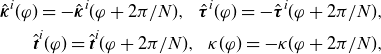 \begin{align} \hat {\boldsymbol {\kappa }}^i(\varphi )=-\hat {\boldsymbol {\kappa }}^i(\varphi +2\pi /N),\ \ \hat {\boldsymbol {\tau }}^i(\varphi )=-\hat {\boldsymbol {\tau }}^i(\varphi +2\pi /N), \nonumber \\ \hat {{\textit{t}}}^i(\varphi )=\hat {{\textit{t}}}^i(\varphi +2\pi /N),\ \ \kappa (\varphi )=-\kappa (\varphi +2\pi /N), \end{align}
where the superscripts denote the cylindrical components of the basis vectors. If it were not for the minus sign, then the frame would be continuous and $2\pi /N$
-periodic, but we see for the half-helicity case that it behaves as if its period was not
$2\pi /N$
-periodic, but we see for the half-helicity case that it behaves as if its period was not $2\pi /N$
, but rather
$2\pi /N$
, but rather $4\pi /N$
. That is, the signed Frenet frame becomes ‘half-periodic’ (i.e. periodic in the extended double-period domain).
$4\pi /N$
. That is, the signed Frenet frame becomes ‘half-periodic’ (i.e. periodic in the extended double-period domain).
A function that is smooth and continuous in the extended domain but has a sign jump in the real domain can generally be written as
 \begin{align} f(\varphi )=-f(\varphi +2\pi /N) \Leftrightarrow f(\varphi )=\tilde {f}_c(\varphi )\cos (N\varphi /2)+\tilde {f}_s(\varphi )\sin (N\varphi /2), \end{align}
where $\tilde {f}_{c/s}$
are smooth and periodic in
$\tilde {f}_{c/s}$
are smooth and periodic in $2\pi /N$
. This form follows from consideration of a function
$2\pi /N$
. This form follows from consideration of a function $f=\cos a\varphi$
and applying the condition that
$f=\cos a\varphi$
and applying the condition that $f(\varphi )=-f(\varphi +2\pi /N)$
, which implies
$f(\varphi )=-f(\varphi +2\pi /N)$
, which implies $a=N/2+nN$
where
$a=N/2+nN$
where $n\in \mathbb {Z}$
.
$n\in \mathbb {Z}$
.
An interesting property of these half-periodic functions is the following: any product of two half-periodic functions, (B.3), is a smooth periodic function. Therefore, in order for $\mathbf {r}$
, (2.2), to be smooth considering (B.2), we need the functions
$\mathbf {r}$
, (2.2), to be smooth considering (B.2), we need the functions $X$
and
$X$
and $Y$
to be half-periodic functions.
$Y$
to be half-periodic functions.
B.1.3 Continuity of first-order construction for half-helicity
Let us consider the first-order construction in the context of the requirements above. At this order, see figure 1, the functions $X_1$
and
$X_1$
and $B_1$
are the first to appear. We have just argued that the former must be a half-period function, while the latter should not because it is a physical quantity. Following Garren & Boozer (Reference Garren and Boozer1991
Reference Garren and Boozerb
), Plunk et al. (Reference Plunk, Landreman and Helander2019) and in particular the prescription in Camacho-Mata & Plunk (Reference Camacho-Mata and Plunk2023), we write
$B_1$
are the first to appear. We have just argued that the former must be a half-period function, while the latter should not because it is a physical quantity. Following Garren & Boozer (Reference Garren and Boozer1991
Reference Garren and Boozerb
), Plunk et al. (Reference Plunk, Landreman and Helander2019) and in particular the prescription in Camacho-Mata & Plunk (Reference Camacho-Mata and Plunk2023), we write
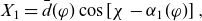 \begin{align} X_1=\bar {d}(\varphi )\cos \left [\chi -\alpha _1(\varphi )\right ], \end{align}
where $\chi =\theta -M\varphi$
, and
$\chi =\theta -M\varphi$
, and $M$
is the half-helicity of the signed frame. As shown in Section 5 of Camacho-Mata & Plunk (Reference Camacho-Mata and Plunk2023), the periodicity of
$M$
is the half-helicity of the signed frame. As shown in Section 5 of Camacho-Mata & Plunk (Reference Camacho-Mata and Plunk2023), the periodicity of $\alpha _1$
and
$\alpha _1$
and $\bar {d}$
are sufficient to ensure that
$\bar {d}$
are sufficient to ensure that $X_1({-}\pi /N)=-X_1(\pi /N)$
. Here we can go further and claim this condition for all derivatives, simply by recognising that as written,
$X_1({-}\pi /N)=-X_1(\pi /N)$
. Here we can go further and claim this condition for all derivatives, simply by recognising that as written, $X_1$
is a half-periodic function, (B.3).
$X_1$
is a half-periodic function, (B.3).
Now, we must make sure that the magnetic field magnitude is continuous and periodic. From (A22) in Landreman & Sengupta (Reference Landreman and Sengupta2019),
 \begin{align} B_1=\kappa X_1 B_0, \end{align}
where we recall that $\kappa$
is the signed curvature, which is also a half-periodic function. We have already seen that the product of two half-period functions is periodic, and thus so is
$\kappa$
is the signed curvature, which is also a half-periodic function. We have already seen that the product of two half-period functions is periodic, and thus so is $B_1$
.
$B_1$
.
To complete the picture at first order (see figure 1) it suffices to check that the same argument as for $X_1$
holds for
$X_1$
holds for $Y_1$
.Footnote 11 Thus, the prescription of Camacho-Mata & Plunk (Reference Camacho-Mata and Plunk2023) does indeed guarantee the correct behaviour of the near-axis construction to first order. Like for quasisymmetric stellarators (Landreman & Sengupta Reference Landreman and Sengupta2019; Rodríguez et al., Reference Rodríguez, Sengupta and Bhattacharjee2022), the helical angle
$Y_1$
.Footnote 11 Thus, the prescription of Camacho-Mata & Plunk (Reference Camacho-Mata and Plunk2023) does indeed guarantee the correct behaviour of the near-axis construction to first order. Like for quasisymmetric stellarators (Landreman & Sengupta Reference Landreman and Sengupta2019; Rodríguez et al., Reference Rodríguez, Sengupta and Bhattacharjee2022), the helical angle $\chi$
is particularly convenient to use as `poloidal’ angle respect to which the harmonic content in the near-axis expansion is defined. For the half-periodic
$\chi$
is particularly convenient to use as `poloidal’ angle respect to which the harmonic content in the near-axis expansion is defined. For the half-periodic $X_1$
and
$X_1$
and $Y_1$
this means that
$Y_1$
this means that $X_{1c}$
,
$X_{1c}$
, $Y_{1s}$
, etc. are periodic in the near-axis equilibrium equations of Landreman & Sengupta (Reference Landreman and Sengupta2019). This proves convenient when proceeding to second order in the expansion as well.
$Y_{1s}$
, etc. are periodic in the near-axis equilibrium equations of Landreman & Sengupta (Reference Landreman and Sengupta2019). This proves convenient when proceeding to second order in the expansion as well.
Before moving to next order, we summarise the periodicity and parity of the first-order functions in table 1.
Periodicity and parity of first-order near-axis. Table summarising the parity of the first-order near-axis expansion and whether they are of the half-periodic type or not. The parity is here considered respect to the centre of the domain (the bottom of the well), with the superscript $^o$
indicating that the parity applies to the point of odd curvature; note that the opposite parity applies at the edges of the domain in a half-helicity scenario. The functions correspond to the
$^o$
indicating that the parity applies to the point of odd curvature; note that the opposite parity applies at the edges of the domain in a half-helicity scenario. The functions correspond to the $\chi$
-harmonics of
$\chi$
-harmonics of $X_1$
,
$X_1$
, $Y_1$
and
$Y_1$
and $B_1$
.
$B_1$
.
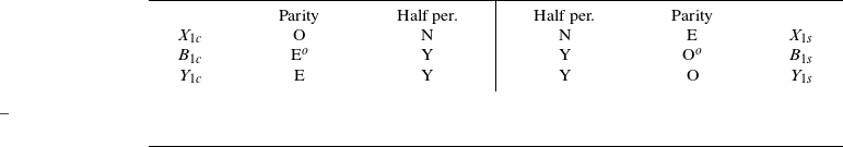
B.1.4 Continuity of second-order construction: half-helicity
Let us continue the construction to second order. Following the flow of the construction in figure 2, the first element to consider is $B_\psi$
which is directly connected to
$B_\psi$
which is directly connected to $B$
and
$B$
and $p$
through magnetohydrostatic (MHS) equilibrium. Although these are physical quantities, resolving the function in harmonics of the newly defined
$p$
through magnetohydrostatic (MHS) equilibrium. Although these are physical quantities, resolving the function in harmonics of the newly defined $\chi =\theta -M\varphi$
(see first-order discussion) makes functions
$\chi =\theta -M\varphi$
(see first-order discussion) makes functions $B_{1c}$
and
$B_{1c}$
and $B_{1s}$
half-periodic (see table 1). Thus, so will the harmonics of
$B_{1s}$
half-periodic (see table 1). Thus, so will the harmonics of $B_\psi$
.
$B_\psi$
.
To construct the function $Z$
next we only need first-order periodic quantities, with which all harmonics of
$Z$
next we only need first-order periodic quantities, with which all harmonics of $Z$
are smooth and periodic. Note that resolving
$Z$
are smooth and periodic. Note that resolving $Z$
in
$Z$
in $\chi$
-harmonics does not introduce the half-periodicity issues of
$\chi$
-harmonics does not introduce the half-periodicity issues of $B_{\psi 1}$
or
$B_{\psi 1}$
or $B_1$
. The reason is that at second order, harmonics involve
$B_1$
. The reason is that at second order, harmonics involve $2\chi =2\theta -2M\varphi$
, which becomes periodic under a sine or cosine. This points to a potential issue that arises at second order with the other elements,
$2\chi =2\theta -2M\varphi$
, which becomes periodic under a sine or cosine. This points to a potential issue that arises at second order with the other elements, $X_2$
and
$X_2$
and $Y_2$
, describing flux surfaces. Unlike at first order, the convenient definition of
$Y_2$
, describing flux surfaces. Unlike at first order, the convenient definition of $\alpha _1$
cannot account for the necessary half-periodicity of the harmonics. We must impose the half-periodic behaviour more explicitly.
$\alpha _1$
cannot account for the necessary half-periodicity of the harmonics. We must impose the half-periodic behaviour more explicitly.
Consider $X_{2c}$
and
$X_{2c}$
and $X_{2s}$
, which are inputs to the near-axis construction (see figure 2). We must choose these to be half-period functions, but they must also have a particular parity. Through (A34–36) of Landreman & Sengupta (Reference Landreman and Sengupta2019),
$X_{2s}$
, which are inputs to the near-axis construction (see figure 2). We must choose these to be half-period functions, but they must also have a particular parity. Through (A34–36) of Landreman & Sengupta (Reference Landreman and Sengupta2019), $X_2$
components are directly linked to
$X_2$
components are directly linked to $B_2$
, which must satisfy
$B_2$
, which must satisfy $B(\chi, \varphi )=B({-}\chi, -\varphi )$
by virtue of stellarator symmetry. Therefore,
$B(\chi, \varphi )=B({-}\chi, -\varphi )$
by virtue of stellarator symmetry. Therefore, $B_{2c}$
and
$B_{2c}$
and $B_{2s}$
must be even and odd functions of
$B_{2s}$
must be even and odd functions of $\varphi$
, respectively. As
$\varphi$
, respectively. As $\ell ^{\prime}\kappa X_{2c}=B_{2c}+\hat {\mathcal {T}}_c$
, and
$\ell ^{\prime}\kappa X_{2c}=B_{2c}+\hat {\mathcal {T}}_c$
, and $\hat {\mathcal {T}}_c$
can be shown to be even, it must be the case that
$\hat {\mathcal {T}}_c$
can be shown to be even, it must be the case that $X_{2c}$
is odd. Odd parity in addition to its half-periodic nature means that we may generally provide
$X_{2c}$
is odd. Odd parity in addition to its half-periodic nature means that we may generally provide $X_{2c}=\tilde {X}_{2c}^o\cos\! (N\varphi /2)+\tilde {X}_{2s}^e\sin \!(N\varphi /2)$
, where the tilde functions are periodic well defined parity (e-even or o-odd) of
$X_{2c}=\tilde {X}_{2c}^o\cos\! (N\varphi /2)+\tilde {X}_{2s}^e\sin \!(N\varphi /2)$
, where the tilde functions are periodic well defined parity (e-even or o-odd) of $\varphi$
. The product through
$\varphi$
. The product through $\kappa$
, as it occurred at first order, guarantees the consistency of
$\kappa$
, as it occurred at first order, guarantees the consistency of $X$
half-period condition with the periodic nature of
$X$
half-period condition with the periodic nature of $B$
. A similar argument follows for
$B$
. A similar argument follows for $X_{2s}$
and
$X_{2s}$
and $B_{2s}$
, but with the parity reversed; i.e.
$B_{2s}$
, but with the parity reversed; i.e. $X_{2s}$
must be even and
$X_{2s}$
must be even and $B_{2s}$
odd.
$B_{2s}$
odd.
The next elements in the construction are $X_{20}$
and
$X_{20}$
and $Y_{20}$
, which are the solutions to the system of equations comprising (A41–48) in Landreman & Sengupta (Reference Landreman and Sengupta2019). Term by term, one can be assured that the solution to the system of equations will be a half-period function provided that the prescription so far followed is continued. This means that we cannot exploit periodicity in solving this system of coupled ODEs. In particular, if we attempt a solution of the system of ODEs as the solution of the linear system
$Y_{20}$
, which are the solutions to the system of equations comprising (A41–48) in Landreman & Sengupta (Reference Landreman and Sengupta2019). Term by term, one can be assured that the solution to the system of equations will be a half-period function provided that the prescription so far followed is continued. This means that we cannot exploit periodicity in solving this system of coupled ODEs. In particular, if we attempt a solution of the system of ODEs as the solution of the linear system $({\boldsymbol{D}}+{\boldsymbol{A}})\mathbf {x}=\mathbf {c}$
where
$({\boldsymbol{D}}+{\boldsymbol{A}})\mathbf {x}=\mathbf {c}$
where $\mathbf {x}$
contains the values of functions
$\mathbf {x}$
contains the values of functions $X_{20}$
and
$X_{20}$
and $Y_{20}$
on regularly spaced collocation points, we cannot use pseudospectral matrices (Weideman & Reddy Reference Weideman and Reddy2000) like in Landreman & Sengupta (Reference Landreman and Sengupta2019) to solve the problem. We can nevertheless extend the treatment by defining the following pseudospectral differentiation matrix for equally spaced grid points of a half-periodic function,
$Y_{20}$
on regularly spaced collocation points, we cannot use pseudospectral matrices (Weideman & Reddy Reference Weideman and Reddy2000) like in Landreman & Sengupta (Reference Landreman and Sengupta2019) to solve the problem. We can nevertheless extend the treatment by defining the following pseudospectral differentiation matrix for equally spaced grid points of a half-periodic function,
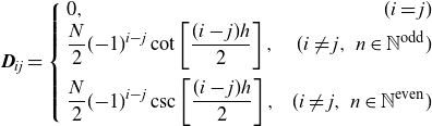 \begin{align} {{\textit{D}}}_{ij}=\begin{cases} \begin{aligned} &0, & (i=j) \\ &\frac {N}{2}({-}1)^{i-j}\cot \left [\frac {(i-j)h}{2}\right ], & (i\neq j,\ n\in \mathbb {N}^{\mathrm {odd}}) \\[5pt] &\frac {N}{2}({-}1)^{i-j}\csc \left [\frac {(i-j)h}{2}\right ], & (i\neq j,\ n\in \mathbb {N}^{\mathrm {even}}) \end{aligned} \end{cases} \end{align}
for $n$
the number of evenly spaced grid points and
$n$
the number of evenly spaced grid points and $h=2\pi /n$
.
$h=2\pi /n$
.
Once the system of equations is solved using this correct definition of ${\boldsymbol{D}}$
, the final step in the second-order construction (see figure 2) is straightforward. The algebraic operations can be seen to preserve the right half-periodic behaviour of
${\boldsymbol{D}}$
, the final step in the second-order construction (see figure 2) is straightforward. The algebraic operations can be seen to preserve the right half-periodic behaviour of $Y_{2c}$
and
$Y_{2c}$
and $Y_{2s}$
, while preserving the periodic nature of
$Y_{2s}$
, while preserving the periodic nature of $B_{20}$
through multiplication by
$B_{20}$
through multiplication by $\kappa$
. We have therefore shown that a consistent construction to second order is possible for half-helicity fields. We summarise the periodicity and parity of the second-order functions in table 2.
$\kappa$
. We have therefore shown that a consistent construction to second order is possible for half-helicity fields. We summarise the periodicity and parity of the second-order functions in table 2.
Periodicity and parity of second-order near-axis. Table summarising the parity of the second-order near-axis expansion and whether they are of the half-periodic type or not. The parity is here considered respect to the centre of the domain (the bottom of the well), with the superscript $^o$
denoting the different parity across the edges of the domain in a half-helicity scenario.
$^o$
denoting the different parity across the edges of the domain in a half-helicity scenario.
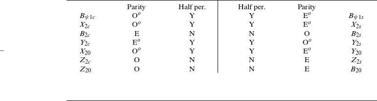
A final comment should be devoted to the scenario at third order. We only need third-order elements when it comes to constructing a description of the equilibrium boundary when the near-axis is used to construct global equilibria. This is important in § 4, the numerical comparison. The details and procedure can be found in Section 3 of Landreman & Sengupta (Reference Landreman and Sengupta2019), and here we must make sure that the shapes constructed following that are continuous and smooth. The answer is affirmative, as it is only the $\chi$
(and not
$\chi$
(and not $3\chi$
) harmonics that are needed to be non-zero, and the same way that the first order
$3\chi$
) harmonics that are needed to be non-zero, and the same way that the first order $X_1$
and
$X_1$
and $Y_1$
were well behaved, so are these. The procedure needs no change to accommodate the half-helicity problem.
$Y_1$
were well behaved, so are these. The procedure needs no change to accommodate the half-helicity problem.
B.2 Continuity of buffer region
We refer as buffer regions to the parts of the toroidal domain (which must include $B_{{max}}$
) in which a controlled deviation from QI is allowed for. This is a first-order near-axis notion (Plunk et al. Reference Plunk, Landreman and Helander2019; Camacho Mata et al. Reference Camacho Mata, Plunk and Jorge2022) arising from a clash between omnigeneity and the periodicity requirement of the field. Let us see how it arises and how it can be managed in a controlled way.
$B_{{max}}$
) in which a controlled deviation from QI is allowed for. This is a first-order near-axis notion (Plunk et al. Reference Plunk, Landreman and Helander2019; Camacho Mata et al. Reference Camacho Mata, Plunk and Jorge2022) arising from a clash between omnigeneity and the periodicity requirement of the field. Let us see how it arises and how it can be managed in a controlled way.
To this end, let us start by writing the first-order field as $B_1=\bar {d}\kappa \cos\! (\chi -\alpha _1)$
. In order to make the field periodic, we define here
$B_1=\bar {d}\kappa \cos\! (\chi -\alpha _1)$
. In order to make the field periodic, we define here $\chi =\theta -M\varphi$
with
$\chi =\theta -M\varphi$
with $M$
being the helicity of the axis (which we may take to be an integer for simplicity), and
$M$
being the helicity of the axis (which we may take to be an integer for simplicity), and $\bar {d}$
and
$\bar {d}$
and $\alpha _1$
as periodic functions.Footnote 12 The additional constraint of stellarator symmetry requires
$\alpha _1$
as periodic functions.Footnote 12 The additional constraint of stellarator symmetry requires $\bar {d}$
to be even and
$\bar {d}$
to be even and $\alpha _1=\tilde {\alpha }-\pi /2$
, where
$\alpha _1=\tilde {\alpha }-\pi /2$
, where $\tilde {\alpha }$
is an odd, periodic function. Finally, we have the QI conditions (Plunk et al. (Reference Plunk, Landreman and Helander2019); Rodríguez & Plunk (Reference Rodríguez and Plunk2023), (31)) which require
$\tilde {\alpha }$
is an odd, periodic function. Finally, we have the QI conditions (Plunk et al. (Reference Plunk, Landreman and Helander2019); Rodríguez & Plunk (Reference Rodríguez and Plunk2023), (31)) which require
 \begin{align} \alpha _1^{\mathrm {QI}}=\bar {\iota }_0\varphi -\pi /2. \end{align}
But clearly simply setting $\alpha _1 = \alpha _1^{\mathrm {QI}}$
violates periodicity, unless
$\alpha _1 = \alpha _1^{\mathrm {QI}}$
violates periodicity, unless $\bar {\iota }_0=\iota _0-M=0$
, which is generally not true. This is why it is generally not possible to grant QI exactly. For an approximate QI field, we need the choice of an odd periodic
$\bar {\iota }_0=\iota _0-M=0$
, which is generally not true. This is why it is generally not possible to grant QI exactly. For an approximate QI field, we need the choice of an odd periodic $\tilde {\alpha }$
that is close to the ideal QI behaviour, (B.7).
$\tilde {\alpha }$
that is close to the ideal QI behaviour, (B.7).
B.2.1 Piecewise buffer
The first approach considered in the literature to construct $\tilde {\alpha }$
can be found in Plunk et al. (Reference Plunk, Landreman and Helander2019). The periodic function is defined as a piecewise function,
$\tilde {\alpha }$
can be found in Plunk et al. (Reference Plunk, Landreman and Helander2019). The periodic function is defined as a piecewise function,
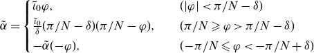 \begin{align} \tilde {\alpha }=\begin{cases} \bar {\iota }_0\varphi, \quad & (|\varphi |\lt \pi /N-\delta ) \\[3pt] \frac {\bar {\iota }_0}{\delta }(\pi /N-\delta )(\pi /N-\varphi ), \quad & (\pi /N\geqslant \varphi \gt \pi /N-\delta ) \\[3pt] -\tilde {\alpha }({-}\varphi ), \quad & ({-}\pi /N\leqslant \varphi \lt -\pi /N+\delta ) \end{cases} \end{align}
where the central region of the domain is exactly omnigeneous, and the breakup is restricted to narrow regions of width $\delta$
at the edges (input parameter). The piecewise function is
$\delta$
at the edges (input parameter). The piecewise function is $C^0$
, with the derivative being discontinuous at the joints of the domain. This lack of smoothness leads to an impossibility to proceed to second order, where the field becomes discontinuous. In addition, and as studied in Camacho Mata et al. (Reference Camacho Mata, Plunk and Jorge2022), the edge and the core being decoupled in this way leads to large variations in the field within the edge buffer, where the field needs to make, within a narrow space, the necessary corrections for a consistent field. Note that we have chosen a convention different from the original work of Camacho Mata et al. (Reference Camacho Mata, Plunk and Jorge2022), where
$C^0$
, with the derivative being discontinuous at the joints of the domain. This lack of smoothness leads to an impossibility to proceed to second order, where the field becomes discontinuous. In addition, and as studied in Camacho Mata et al. (Reference Camacho Mata, Plunk and Jorge2022), the edge and the core being decoupled in this way leads to large variations in the field within the edge buffer, where the field needs to make, within a narrow space, the necessary corrections for a consistent field. Note that we have chosen a convention different from the original work of Camacho Mata et al. (Reference Camacho Mata, Plunk and Jorge2022), where $\tilde {\alpha }=0$
at
$\tilde {\alpha }=0$
at $\varphi =0$
(our bottom of the well), instead of
$\varphi =0$
(our bottom of the well), instead of $(2M/N+1)\pi$
.
$(2M/N+1)\pi$
.
B.2.2 Standard buffer
Recognising the limitations of the above, in the recent work by Camacho Mata et al. (Reference Camacho Mata, Plunk and Jorge2022), a construction was presented which attempted a more smooth distribution of the buffer. In our present notation, that construction may be written as
 \begin{align} \tilde {\alpha } = \bar {\iota }_0\frac {\pi }{N}\left [\frac {\varphi }{\pi /N}-\left (\frac {\varphi }{\pi /N}\right )^{2k+1}\right ], \end{align}
which is as needed an odd function of $\varphi$
with the correct QI behaviour near
$\varphi$
with the correct QI behaviour near $\varphi \sim 0$
. The order
$\varphi \sim 0$
. The order $k\gt 0$
denotes the number of derivatives (
$k\gt 0$
denotes the number of derivatives ( $2k+1$
) that
$2k+1$
) that $\tilde {\alpha }$
match the ideal QI form (B.7) near the centre of the domain. The larger
$\tilde {\alpha }$
match the ideal QI form (B.7) near the centre of the domain. The larger $k$
is, the larger the central region of agreement, and thus the narrower the region with a significant deviation at the edges. To avoid some of the problems of the piecewise construction, typical values of
$k$
is, the larger the central region of agreement, and thus the narrower the region with a significant deviation at the edges. To avoid some of the problems of the piecewise construction, typical values of $k=2$
or
$k=2$
or $3$
are appropriate (Camacho Mata et al. Reference Camacho Mata, Plunk and Jorge2022; Camacho-Mata & Plunk Reference Camacho-Mata and Plunk2023). We call this construction the standard buffer.
$3$
are appropriate (Camacho Mata et al. Reference Camacho Mata, Plunk and Jorge2022; Camacho-Mata & Plunk Reference Camacho-Mata and Plunk2023). We call this construction the standard buffer.
Although the function is not piecewise, it is not smooth in the periodic domain either. The lack of smoothness is localised at the edges, $\varphi =\pm \pi /N$
, where
$\varphi =\pm \pi /N$
, where $\cos \tilde {\alpha }$
and
$\cos \tilde {\alpha }$
and $\sin \tilde {\alpha }$
are
$\sin \tilde {\alpha }$
are $C^2$
and
$C^2$
and $C^1$
, respectively. This means that first-order field quantities such as
$C^1$
, respectively. This means that first-order field quantities such as $B_1$
or
$B_1$
or $X_1$
will be clearly non-smooth.Footnote 13 In fact, the lack of smoothness is so readily observed that second-order field quantities will be unphysically discontinuous. Let us show this briefly.
$X_1$
will be clearly non-smooth.Footnote 13 In fact, the lack of smoothness is so readily observed that second-order field quantities will be unphysically discontinuous. Let us show this briefly.
Consider explicitly the evaluation of $B_{2s}$
, which directly depends on the derivative of
$B_{2s}$
, which directly depends on the derivative of $Z_{2s}$
, and as such, see figure 2, involves second derivatives of first-order quantities as
$Z_{2s}$
, and as such, see figure 2, involves second derivatives of first-order quantities as
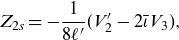 \begin{align} Z_{2s}=-\frac {1}{8\ell ^{\prime}}(V_2^{\prime}-2\bar {\iota }V_3), \end{align}
where
 \begin{align} V_2&=2[X_{1c}X_{1s}+Y_{1c}Y_{1s}], \\[-9pt] \nonumber \end{align}
 \begin{align} V_3 & = X_{1c}^2-X_{1s}^2+Y_{1c}^2-Y_{1s}^2. \\[6pt] \nonumber \end{align}
It can be shown through the explicit calculation of the dependence on $\tilde {\alpha }$
that
$\tilde {\alpha }$
that $V_3\in C^2$
and
$V_3\in C^2$
and $V_2\in C^1$
, so that
$V_2\in C^1$
, so that $Z_{2s}\in C^0$
, i.e. just about continuous. From (A35) in Landreman & Sengupta (Reference Landreman and Sengupta2019), one may relate
$Z_{2s}\in C^0$
, i.e. just about continuous. From (A35) in Landreman & Sengupta (Reference Landreman and Sengupta2019), one may relate $B_{2s}\sim Z_{2s}^{\prime}$
, meaning that the function
$B_{2s}\sim Z_{2s}^{\prime}$
, meaning that the function $B_{2s}$
is generally discontinuous (and non-symmetric) at the endpoints of the periodic domain. See figure 3 for an example of this. A similar argument shows that the other components of
$B_{2s}$
is generally discontinuous (and non-symmetric) at the endpoints of the periodic domain. See figure 3 for an example of this. A similar argument shows that the other components of $B$
are continuous, as well as the
$B$
are continuous, as well as the $X_2$
ad
$X_2$
ad $Y_2$
components.Footnote 14 Although the discontinuity limits the physicality of the second-order field, it occurs in a rather controlled fashion, as can also be seen in the example of figure 3.
$Y_2$
components.Footnote 14 Although the discontinuity limits the physicality of the second-order field, it occurs in a rather controlled fashion, as can also be seen in the example of figure 3.
The lack of smoothness can, however, limit some of the numerical procedures in the problem, such as the use of pseudospectral methods to solve ODEs, which rely on the assumption of periodicity and smoothness. In that case, even adopting the upgraded version of this buffer also presented in Camacho Mata et al. (Reference Camacho Mata, Plunk and Jorge2022), which raises the order of differentiability further, would be potentially problematic. It is typical to expect Gibb’s-like phenomena.
B.2.3 Smooth buffer
Following the previous discussion, it is natural to seek the construction of a buffer that is smooth everywhere and yet similar to functions like that of (B.9). Generally, we shall write $\tilde {\alpha }$
, which must be an odd, periodic, smooth function, as a sine Fourier series.
$\tilde {\alpha }$
, which must be an odd, periodic, smooth function, as a sine Fourier series.
Following the construction of the standard buffer, § B.2.2, we impose the following $k$
constraints that attempt to match
$k$
constraints that attempt to match $\tilde {\alpha }$
to its ideal QI form near
$\tilde {\alpha }$
to its ideal QI form near $\varphi =0$
:
$\varphi =0$
:
 \begin{align} \begin{cases} \begin{aligned} &\frac {\partial \tilde {\alpha }}{\partial \varphi }=\bar {\iota }_0, \\[3pt] &\left (\frac {\partial }{\partial \varphi }\right )^{2j+1}\tilde {\alpha }=0,\quad (1\lt j\leqslant k) \end{aligned} \end{cases} \end{align}
and everything is evaluated at $\varphi =0$
. The larger
$\varphi =0$
. The larger $k$
, the larger the number of derivatives near the origin that match the ideal QI case.
$k$
, the larger the number of derivatives near the origin that match the ideal QI case.
To satisfy these $k$
constraints uniquely, we restrict the sine Fourier series to the first
$k$
constraints uniquely, we restrict the sine Fourier series to the first $k$
harmonics, so that the conditions above reduce to a linear system of algebraic equations. Defining the vector
$k$
harmonics, so that the conditions above reduce to a linear system of algebraic equations. Defining the vector $\mathbf {a}$
as the one-indexed vector of Fourier coefficients, we may write
$\mathbf {a}$
as the one-indexed vector of Fourier coefficients, we may write
 \begin{align} \mathbf {a}_i=\frac {\bar {\iota }}{N}{{\boldsymbol{S}}}^{-1}_{i1}, \end{align}
where the matrix,
 \begin{align} {{\boldsymbol{S}}}_{ij}=({-}1)^{i+1}j^{2i+1}. \end{align}
That is, the first column of the inverse of ${\boldsymbol{S}}$
. At large
${\boldsymbol{S}}$
. At large $k$
(for
$k$
(for $k\gt 9$
in practice) the inversion of the matrix becomes problematic numerically due to the large discrepancy in magnitude in the matrix elements due to the strong exponential term.
$k\gt 9$
in practice) the inversion of the matrix becomes problematic numerically due to the large discrepancy in magnitude in the matrix elements due to the strong exponential term.
Given the similarities of this buffer construction with the standard one, § B.2.2, we may ask how they compare. For this comparison, we define an effective size of the buffer region as the fraction of the domain where the QI deviation is significant. In particular, we take the turning points where $\tilde {\alpha }^\prime = 0$
as measure. The comparison is shown in table 3. The smooth buffer struggles to narrow the buffer region down, and does so at the expense of a high harmonic content. Nevertheless, following the prescription of Camacho Mata et al. (Reference Camacho Mata, Plunk and Jorge2022), a reasonable choice of parameter would be
$\tilde {\alpha }^\prime = 0$
as measure. The comparison is shown in table 3. The smooth buffer struggles to narrow the buffer region down, and does so at the expense of a high harmonic content. Nevertheless, following the prescription of Camacho Mata et al. (Reference Camacho Mata, Plunk and Jorge2022), a reasonable choice of parameter would be $k=5$
for the smooth buffer (which we may also call Fourier buffer). Other alternatives could also be concocted, but these suffice.
$k=5$
for the smooth buffer (which we may also call Fourier buffer). Other alternatives could also be concocted, but these suffice.
Effective size of the buffer region. Table comparing the effective size of the buffer region (fraction of the domain) for different values of the parameter $k$
between the smooth and standard constructions.
$k$
between the smooth and standard constructions.
Appendix C. Deviation from omnigeneity at second order
This appendix presents an assessment of the level of omnigeneity breaking at second order in the near-axis expansion, taking into account its necessary violation at first order. An understanding of these deviations will resolve the toroidal extent about the minimum of the well in which it is meaningful to enforce the QI conditions at second order. This appendix draws heavily on the machinery developed in Rodríguez & Plunk (Reference Rodríguez and Plunk2023), of which a certain level of familiarity is assumed. The most essential elements are included here, but the reader is referred to the aforementioned paper for a more thorough and complete account.
Let us start by settling the type of field we are considering here: we focus on stellarator symmetric, single-well fields, of which the bottom of the well is taken to be at $\varphi =0$
. We define omnigeneity as the property of a field which satisfies
$\varphi =0$
. We define omnigeneity as the property of a field which satisfies
 \begin{align} Y(r,\alpha, \varphi ) = Y(r,\alpha, \eta (\varphi )), \end{align}
where
 \begin{align} Y=\frac {\nabla \psi \times \mathbf {B}\cdot \nabla B}{\mathbf {B}\cdot \nabla B}, \end{align}
and $\eta (\varphi )$
is a function that maps pairs of equal
$\eta (\varphi )$
is a function that maps pairs of equal $B$
points on either side of the magnetic well along a field line; i.e.
$B$
points on either side of the magnetic well along a field line; i.e. $B(\alpha, \eta (\varphi ))=B(\alpha, \varphi )$
and
$B(\alpha, \eta (\varphi ))=B(\alpha, \varphi )$
and $\eta (\varphi )\neq \varphi$
except for
$\eta (\varphi )\neq \varphi$
except for $\varphi =0$
and
$\varphi =0$
and $\alpha =\theta -\iota \varphi$
. This description may be interpreted as the condition for the radial magnetic drift displacement of particles to be equal but opposite on either side of the magnetic well.
$\alpha =\theta -\iota \varphi$
. This description may be interpreted as the condition for the radial magnetic drift displacement of particles to be equal but opposite on either side of the magnetic well.
An asymptotic consideration of (C.1) in the distance from the axis and careful consideration order-by-order yields the conditions of QI used in the main body of this paper and derived in Rodríguez & Plunk (Reference Rodríguez and Plunk2023), the lowest order of which were originally obtained in Plunk et al. (Reference Plunk, Landreman and Helander2019). Here, though, we are not interested on rederiving this exact problem. Instead, we want to assess the deviation in (C.1) induced by the existing limitations to achieve omnigeneity exactly. In particular, we shall consider a field that is QI at first order but for the presence of a buffer $\alpha _{\mathrm {buf}}$
,
$\alpha _{\mathrm {buf}}$
,
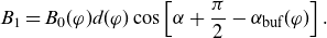 \begin{align} B_1=B_0(\varphi )d(\varphi )\cos \left [\alpha +\frac {\pi }{2}-\alpha _{\mathrm {buf}}(\varphi )\right ]. \end{align}
The field is ideally omnigeneous when $\alpha _{\mathrm {buf}}=0$
provided
$\alpha _{\mathrm {buf}}=0$
provided $d$
is odd (
$d$
is odd ( $B_0$
is even). The buffer must be an odd function of
$B_0$
is even). The buffer must be an odd function of $\varphi$
in order for the field to comply with stellarator symmetry. The presence of the buffer leads to an omnigeneity breaking that we may quantify to leading order
$\varphi$
in order for the field to comply with stellarator symmetry. The presence of the buffer leads to an omnigeneity breaking that we may quantify to leading order $O(r)$
as
$O(r)$
as
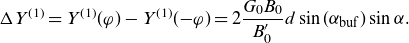 \begin{align} \Delta Y^{(1)}=Y^{(1)}(\varphi )-Y^{(1)}({-}\varphi )=2\frac {G_0B_0}{B_0^{\prime}}d\sin (\alpha _{\mathrm {buf}})\sin \alpha . \end{align}
The procedure may be repeated with the next order, in this case being careful to include the variation in the map $\eta$
due to the variation of
$\eta$
due to the variation of $B$
. Following Rodríguez & Plunk (Reference Rodríguez and Plunk2023), and after significant algebra, we write using the shorthand notation
$B$
. Following Rodríguez & Plunk (Reference Rodríguez and Plunk2023), and after significant algebra, we write using the shorthand notation $s_x=\sin x$
and
$s_x=\sin x$
and $c_x=\cos x$
,
$c_x=\cos x$
,
 \begin{align} \Delta Y^{(2)} & = Y^{(2)}(\varphi )-Y^{(2)}({-}\varphi )-\eta ^{(1)}(\varphi )\left (\partial _\varphi Y^{(1)}\right )({-}\varphi ) \end{align}
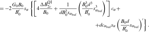 \begin{align} & =-2\frac {G_0B_0}{B_0^{\prime}}s_\alpha \left \{\left [4\frac {\Delta B_{2c}^{\mathrm {QI}}}{B_0}+\frac {1}{dB_0^2s_{\alpha _{\mathrm {buf}}}}\left (\frac {B_0^3d^3}{B_0^{\prime}}s_{\alpha _{\mathrm {buf}}}^3\right )^{\prime}\right ]c_\alpha +\right .\nonumber \\ &\hspace {7cm}\left .+dc_{\alpha _{\mathrm {buf}}}s_\alpha \left (\frac {B_0d}{B_0^{\prime}}s_{\alpha _{\mathrm {buf}}}\right )^{\prime}\right \}. \\[6pt] \nonumber \end{align}
The shorthand $\Delta B_{2c}^{\mathrm {QI}}=B_{2c}^{\mathrm {QI}}-(B_0^2d^2/B_0^{\prime})^{\prime}/4$
is zero when
$\Delta B_{2c}^{\mathrm {QI}}=B_{2c}^{\mathrm {QI}}-(B_0^2d^2/B_0^{\prime})^{\prime}/4$
is zero when $B_{2c}^{\mathrm {QI}}$
assumes its ideal QI form. Putting all together, we may write
$B_{2c}^{\mathrm {QI}}$
assumes its ideal QI form. Putting all together, we may write
 \begin{align} \Delta Y\approx 8r\frac {G_0B_0}{B_0^{\prime}}s_\alpha \Biggl \{\underbrace {\frac {ds_{\alpha _{\mathrm {buf}}}}{4}}_{\mathcal {Y}_0}+rc_\alpha \left [\frac {\Delta B_{2c}^{\mathrm {QI}}}{B_0}+\mathcal {Y}_1\right ]+rs_\alpha \mathcal {Y}_2\Biggr \} + O(r^3), \end{align}
where $\mathcal {Y}_i$
for
$\mathcal {Y}_i$
for $i=1,2$
may be directly read off (C.6). As it must be the case following the conditions of omnigeneity, when
$i=1,2$
may be directly read off (C.6). As it must be the case following the conditions of omnigeneity, when $\alpha _{\mathrm {buf}}=0$
, the omnigeneity condition reduces to
$\alpha _{\mathrm {buf}}=0$
, the omnigeneity condition reduces to $\Delta B_{2c}^{\mathrm {QI}}=0$
. When we acknowledge our impossibility to satisfy QI exactly at first order in the near-axis expansion, there are multiple contributors to omnigeneity breaking at second order. Insisting on the second order QI condition, namely
$\Delta B_{2c}^{\mathrm {QI}}=0$
. When we acknowledge our impossibility to satisfy QI exactly at first order in the near-axis expansion, there are multiple contributors to omnigeneity breaking at second order. Insisting on the second order QI condition, namely $\Delta B_{2c}^{\mathrm {QI}}=0$
, would only make sense in such a scenario if the other terms in (C.7), each with their own
$\Delta B_{2c}^{\mathrm {QI}}=0$
, would only make sense in such a scenario if the other terms in (C.7), each with their own $\alpha$
dependence, are sufficiently small; i.e. the other terms (which solely depend on first-order quantities) serve as meaningful thresholds for
$\alpha$
dependence, are sufficiently small; i.e. the other terms (which solely depend on first-order quantities) serve as meaningful thresholds for $\Delta B_{2c}^{\mathrm {QI}}/B_0$
.
$\Delta B_{2c}^{\mathrm {QI}}/B_0$
.
It is reasonable to assess all of these contributions near the bottom of the well, where $\alpha _{\mathrm {buf}}\approx 0$
, and thus we expect the QI breaking terms to be small. In fact, taking near the bottom of the well
$\alpha _{\mathrm {buf}}\approx 0$
, and thus we expect the QI breaking terms to be small. In fact, taking near the bottom of the well $d\sim \varphi ^v$
,
$d\sim \varphi ^v$
, $B_0^{\prime}\sim \varphi ^{u-1}$
and
$B_0^{\prime}\sim \varphi ^{u-1}$
and $\alpha _{\mathrm {buf}}\sim \varphi ^{2k+3}$
,Footnote 15 we have
$\alpha _{\mathrm {buf}}\sim \varphi ^{2k+3}$
,Footnote 15 we have
 \begin{align} I[\mathcal {Y}_0] = 2k+3+v, \quad I[\mathcal {Y}_1] = 2(2k+3+v)-u, \quad I[\mathcal {Y}_2] = 2k+3+2v-u, \end{align}
where $I[f]$
denotes the power of
$I[f]$
denotes the power of $\varphi$
of the function
$\varphi$
of the function $f$
near
$f$
near $\varphi =0$
. In this context, to respect QI to the level allowed by the breaking of QI at first order, it is reasonable to require
$\varphi =0$
. In this context, to respect QI to the level allowed by the breaking of QI at first order, it is reasonable to require $I[\Delta B_{2c}^{\mathrm {QI}}]\geqslant \min _{n\in \{0,1,2\}}\{I[\mathcal {Y}_n]\}$
, because otherwise the breaking at second order would be larger than that inherited from the first-order violation of QI in the neighbourhood of
$I[\Delta B_{2c}^{\mathrm {QI}}]\geqslant \min _{n\in \{0,1,2\}}\{I[\mathcal {Y}_n]\}$
, because otherwise the breaking at second order would be larger than that inherited from the first-order violation of QI in the neighbourhood of $\varphi = 0$
.
$\varphi = 0$
.
To proceed further, we must say something regarding the indices $u,\ v$
and
$u,\ v$
and $k$
. The constraint of omnigeneity at the bottom of the well imposes severe constraints in
$k$
. The constraint of omnigeneity at the bottom of the well imposes severe constraints in $u$
and
$u$
and $v$
(Rodríguez & Plunk, Reference Rodríguez and Plunk2023). If
$v$
(Rodríguez & Plunk, Reference Rodríguez and Plunk2023). If $u$
is very large, and thus the leading-order field is very flat near the bottom of the well, the first-order perturbation can easily lead to the appearance of defects in the magnetic field; i.e. a topological change in the contours near the bottom, which were called puddles in Rodríguez & Plunk (Reference Rodríguez and Plunk2023). This immediately leads to deconfinement of deeply trapped particles, and thus the requirement of omnigeneity at first order requires
$u$
is very large, and thus the leading-order field is very flat near the bottom of the well, the first-order perturbation can easily lead to the appearance of defects in the magnetic field; i.e. a topological change in the contours near the bottom, which were called puddles in Rodríguez & Plunk (Reference Rodríguez and Plunk2023). This immediately leads to deconfinement of deeply trapped particles, and thus the requirement of omnigeneity at first order requires $2v\geqslant u$
, and only equal in the special case
$2v\geqslant u$
, and only equal in the special case $(u,v)=(2,1)$
. With this constraint in mind,
$(u,v)=(2,1)$
. With this constraint in mind, $I[\mathcal {Y}_1]\geqslant I[\alpha _{\mathrm {buf}}^2]$
and
$I[\mathcal {Y}_1]\geqslant I[\alpha _{\mathrm {buf}}^2]$
and $I[\mathcal {Y}_2]\geqslant I[\alpha _{\mathrm {buf}}]$
, so that the contribution of
$I[\mathcal {Y}_2]\geqslant I[\alpha _{\mathrm {buf}}]$
, so that the contribution of $\mathcal {Y}_1$
may be neglected close to the bottom of the well. Thus, we are left with
$\mathcal {Y}_1$
may be neglected close to the bottom of the well. Thus, we are left with $I[\Delta B_{2c}^{\mathrm {QI}}]\geqslant I[\alpha _{\mathrm {buf}}]+\min \{v,2v-u\}$
, meaning that, at least, it is reasonable to impose the second-order QI condition in the region where the buffer is weak.
$I[\Delta B_{2c}^{\mathrm {QI}}]\geqslant I[\alpha _{\mathrm {buf}}]+\min \{v,2v-u\}$
, meaning that, at least, it is reasonable to impose the second-order QI condition in the region where the buffer is weak.
A more quantitative measure of the extent of the region near the bottom can be obtained by computing $\mathcal {Y}_n$
functions explicitly. Note, though, that an interpretation of what a ‘reasonable’ absolute value of this term is will depend on the precise features about an omnigeneous field that one seeks. Different considerations (say neoclassical transport through
$\mathcal {Y}_n$
functions explicitly. Note, though, that an interpretation of what a ‘reasonable’ absolute value of this term is will depend on the precise features about an omnigeneous field that one seeks. Different considerations (say neoclassical transport through $\epsilon _{\mathrm {eff}}$
(Nemov et al. Reference Nemov, Kasilov, Kernbichler and Heyn1999), fast particle confinement (Nemov et al. Reference Nemov, Kasilov, Kernbichler and Leitold2008; Velasco et al. Reference Velasco, Calvo, Mulas, Sánchez, Parra and Cappa2021) or other derived QI properties such as vanishing bootstrap current (Helander & Nührenberg, Reference Helander and Nührenberg2009)) will lead to different measures. We leave that for development in future applications and satisfy ourselves with the simple criterion of satisfying QI in the region where the buffer function is small.
$\epsilon _{\mathrm {eff}}$
(Nemov et al. Reference Nemov, Kasilov, Kernbichler and Heyn1999), fast particle confinement (Nemov et al. Reference Nemov, Kasilov, Kernbichler and Leitold2008; Velasco et al. Reference Velasco, Calvo, Mulas, Sánchez, Parra and Cappa2021) or other derived QI properties such as vanishing bootstrap current (Helander & Nührenberg, Reference Helander and Nührenberg2009)) will lead to different measures. We leave that for development in future applications and satisfy ourselves with the simple criterion of satisfying QI in the region where the buffer function is small.
Appendix D. Explicit form of second-order equations for
$B_2$

In this appendix we reproduce the key equations relating the harmonic components of $B_2$
and
$B_2$
and $X_2$
for reference. We do so instead of simply referring to LS due to the important role played by these equations. Reading off (A35) and (A36) in LS,
$X_2$
for reference. We do so instead of simply referring to LS due to the important role played by these equations. Reading off (A35) and (A36) in LS,
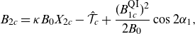 \begin{align} B_{2c} = \kappa B_0X_{2c}-\hat {\mathcal {T}}_c+\frac {(B_{1c}^{\mathrm {QI}})^2}{2B_0}\cos 2\alpha _1, \\[-24pt] \nonumber \end{align}
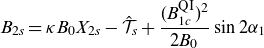 \begin{align} B_{2s}=\kappa B_0X_{2s}-\hat {\mathcal {T}}_s+\frac {(B_{1c}^{\mathrm {QI}})^2}{2B_0}\sin 2\alpha _1 \\[6pt] \nonumber \end{align}
where
 \begin{gather} B_{1c}^{\mathrm {QI}}=B_0\bar {d}\kappa, \\[-24pt] \nonumber \end{gather}
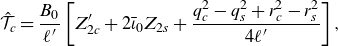 \begin{gather} \hat {\mathcal {T}}_c=\frac {B_0}{\ell ^{\prime}}\left [Z_{2c}^{\prime}+2\bar {\iota }_0 Z_{2s}+\frac {q_c^2-q_s^2+r_c^2-r_s^2}{4\ell ^{\prime}}\right ], \end{gather}
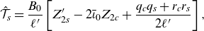 \begin{gather} \hat {\mathcal {T}}_s=\frac {B_0}{\ell ^{\prime}}\left [Z_{2s}^{\prime}-2\bar {\iota }_0 Z_{2c}+\frac {q_cq_s+r_cr_s}{2\ell ^{\prime}}\right ], \\[6pt] \nonumber \end{gather}
and using the notation of (A37)–(A40) in LS,
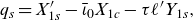 \begin{gather} q_s=X_{1s}^{\prime}-\bar {\iota }_0X_{1c}-\tau \ell ^{\prime}Y_{1s}, \\[-24pt] \nonumber \end{gather}
 \begin{gather} q_c=X_{1c}^{\prime}+\bar {\iota }_0X_{1s}-\tau \ell ^{\prime}Y_{1c}, \\[-24pt] \nonumber \end{gather}
 \begin{gather} r_s=Y_{1s}^{\prime}-\bar {\iota }_0Y_{1c}+\tau \ell ^{\prime}X_{1s}, \\[-24pt] \nonumber \end{gather}
 \begin{gather} r_c=Y_{1c}^{\prime}+\bar {\iota }_0Y_{1s}+\tau \ell ^{\prime}X_{1c}. \\[6pt] \nonumber \end{gather}
The parity of the different terms can be easily traced down by using the information regarding the parity of first and second-order near-axis functions in tables 1 and 2, in addition to $\kappa$
and
$\kappa$
and $\tau$
necessarily being odd and even about the minimum of the well.
$\tau$
necessarily being odd and even about the minimum of the well.
Appendix E. Alternative construction of second-order omnigeneous field
In § 3, we presented a way of constructing an equilibrium field to second order that satisfied omnigeneity to second order. This minimal shaping approach, in an attempt to minimise second-order shaping, considered the simple choice of $X_{2c}=0=X_{2s}$
, and focused on optimising the zeroth- and first-order near-axis choices to satisfy the QI constraints.
$X_{2c}=0=X_{2s}$
, and focused on optimising the zeroth- and first-order near-axis choices to satisfy the QI constraints.
There is naturally an alternative approach, in which the role of the first-order degrees of freedom is minimised, and the second-order shaping exploited as much as possible to satisfy the omnigeneous considerations on $|\mathbf {B}|$
. We call this the omnigeneous completion of the field. To proceed this way, one must follow the following steps.
$|\mathbf {B}|$
. We call this the omnigeneous completion of the field. To proceed this way, one must follow the following steps.
The little control on the second-order shaping of this approach leads, generally and in practice, to near-axis equilibria with large amounts of shaping, which limits the range of validity of the near-axis description itself. This breakdown manifests in the form of non-physically intersecting flux surfaces (Landreman Reference Landreman2021). Thus, we so far generally favour the minimal shaping alternative presented in the main text.
-
(i) Consistency condition: the first step in the construction is to make sure that the constraints at flattening points are satisfied. For a zero of curvature of order
$v$
(that is,
$\kappa \sim \phi ^v$
locally),(E.1)for
\begin{align} \frac {\mathrm {d}^{l}}{\mathrm {d}\varphi ^l}\left [\hat {\mathcal {T}}_c \cos {2\alpha _1}+\hat {\mathcal {T}}_s \sin {2\alpha _1}+\frac {B_0^2}{4}\left (\frac {d^2}{B_0^{\prime}}\right )^{\prime}\right ]_{\varphi =\varphi _c}=0, \end{align}
$l\in \mathbb {N}^{\mathrm {even}}\cup \{0\}$
such that
$0\leqslant l\lt v$
where
$\varphi _c$
represents the flattening point.Footnote 16 These are
$(v+1)/2$
(for
$v$
odd) constraints on lower-order quantities, which may be thought of as constraints on the local values of
$\bar {d}^{(l+2)}$
. This is the only step in which the construction restricts the lower-order near-axis choices. One must find a first-order construction that satisfies these constraints.
-
(ii) Choose the second-order shaping: once the conditions near the flattening points are satisfied, one can then solve (3.6a) for
$\tilde {X}_{2c}$
to find a shaping that enforces the omnigeneous behaviour everywhere. The key observation is that one may always do so provided step one is taken first; otherwise, the construction of
$\tilde {X}_{2c}$
is not well-posed. After choosing
$\tilde {X}_{2c}$
accordingly, the problem still retains some freedom in the choice of
$\tilde {X}_{2s}$
. Besides it being even to preserve stellarator symmetry, it is a free function. -
(iii) Construct second-order field: with these we have all the elements needed to revert (2.7a)–(2.7b), and complete the second-order construction (figure 2).


 Open access