


1. Introduction
Designing successful magnetic-confinement-fusion devices relies on understanding the transport of energy and particles in hot magnetised plasmas. In most modern fusion experiments, the majority of this transport out of the confined region of the plasma is a result of turbulent fluctuations on scales much smaller than the size of the device (and usually associated with the Larmor radius of one or more of the particle species in the plasma). These fluctuations are continuously excited by small-scale instabilities (often called ‘microinstabilities’) driven by the gradients of temperature and density of the large-scale plasma equilibrium. Understanding the conditions for the triggering of these instabilities and how they can be suppressed is therefore of crucial importance for designing devices that can support the larger gradients necessary for higher fusion performance.
Some of the early work on microinstabilities considered a simple inhomogeneous plasma in a straight magnetic field that is either uniform (Rudakov & Sagdeev Reference Rudakov and Sagdeev1961; Coppi et al. Reference Coppi, Furth, Rosenbluth and Sagdeev1966) or sheared (Coppi, Rosenbluth & Sagdeev Reference Coppi, Rosenbluth and Sagdeev1967; Cowley, Kulsrud & Sudan Reference Cowley, Kulsrud and Sudan1991; Newton, Cowley & Loureiro Reference Newton, Cowley and Loureiro2010). Such magnetic-field configurations are often called ‘slabs’ and so these instabilities are known as ‘slab instabilities’. However, the equilibrium magnetic field in magnetic-confinement-fusion devices is never completely straight. There exists a separate class of instabilities, often called ‘curvature-driven’ (or sometimes ‘toroidal’), that rely on the magnetic drifts resulting from the non-uniform magnetic field (Pogutse Reference Pogutse1968; Terry, Anderson & Horton Reference Terry, Anderson and Horton1982; Guzdar et al. Reference Guzdar, Chen, Tang and Rutherford1983; Romanelli Reference Romanelli1989; Biglari, Diamond & Rosenbluth Reference Biglari, Diamond and Rosenbluth1989). By definition, these instabilities do not exist in the slab geometry, sheared or otherwise. In toroidal geometry, one often finds that the corresponding eigenmodes are peaked near the outboard midplane, where the local gradients of the magnetic field and the plasma pressure are aligned. In some simple cases, e.g. the curvature-driven ion-temperature-gradient (cITG) mode, this can be demonstrated by ignoring the parallel variation of the magnetic drifts and solving the dispersion relation in what is sometimes called the ‘local kinetic limit’ (Romanelli Reference Romanelli1989). With this simplification, it is easy to show that cITG modes are unstable when the aforementioned gradients are aligned, and become stable at the inboard side of the device, where the gradients oppose each other (Beer Reference Beer1995). Therefore, magnetic curvature that is aligned with the plasma-pressure gradient is often referred to as ‘bad curvature’, on account of its ability to excite plasma microinstabilities. The same bad magnetic curvature is also responsible for large-scale magnetohydrodynamic (MHD) instabilities (Bateman & Peng Reference Bateman and Peng1977; White Reference White2014), further underscoring its destabilising nature. Analogously, ‘good curvature’ refers to magnetic curvature that points opposite to the pressure gradient.
Combined with the magnetic drifts, trapped particles can also drive linear instabilities. There are various trapped-electron (Adam et al. Reference Adam, Laval and Pellat1973, Reference Adam, Tang and Rutherford1976; Catto & Tsang Reference Catto and Tsang1978; Cheng & Chen Reference Cheng and Chen1981) and trapped-ion (Xu & Rosenbluth Reference Xu and Rosenbluth1991) modes, which are often considered to be important sources of turbulent fluctuations. These instabilities cannot be described using the same local analysis that is applicable to the cITG mode. In axisymmetric geometry, particles are trapped at the outboard, low-field side of the device, which coincides with the bad-curvature region. However, in non-axisymmetric geometry, the trapped-particle and bad-curvature regions may not necessarily overlap. This, combined with the fact that trapped-particle modes are typically only unstable in the bad-curvature regions, underlies some schemes for optimising stellarator configurations (Proll et al. Reference Proll, Helander, Connor and Plunk2012; Helander, Proll & Plunk Reference Helander, Proll and Plunk2013; Rodríguez et al. Reference Rodríguez, Helander and Goodman2024).
In this work, we investigate the properties of gyrokinetic (GK) curvature-driven microinstabilities and their localisation to regions of either good or bad magnetic curvature. Our analysis is based on GK conservation laws and is largely agnostic to the physical mechanisms that destabilise the fluctuations. First, we show that the conservation of a quantity we call the GK field invariant can be used to classify modes as either slab-like or curvature-driven. Furthermore, the evolution equation of this invariant provides a natural definition of good and bad magnetic curvature. Given a few reasonable assumptions (stated in detail in § 2.4), we show that the sign of the field invariant is related to the localisation of the curvature-driven modes to regions of either good or bad magnetic curvature. In the electrostatic limit, the field invariant is negative definite. This allows us to conclude that a large class of electrostatic curvature-driven modes (viz. those satisfying the assumptions of § 2.4), must be localised to regions of bad magnetic curvature. Consequently, we expect that modes driven unstable by good magnetic curvature are electromagnetic.
In the second half of this paper, we present a novel low- $\beta$
, electromagnetic, curvature-driven instability that we call the magnetic-drift mode (MDM) and that is triggered only in good-curvature regions. By comparing it with the well-known electrostatic, curvature-driven electron-temperature-gradient (cETG) instability, we discuss some of the distinctive features of the MDM. We argue that it may be related to some exotic species of microtearing modes seen in GK simulations in toroidal geometry (Jian et al. Reference Jian, Holland, Candy, Ding, Belli, Chan, Staebler, Garofalo, Mcclenaghan and Snyder2021; Patel Reference Patel2021).
$\beta$
, electromagnetic, curvature-driven instability that we call the magnetic-drift mode (MDM) and that is triggered only in good-curvature regions. By comparing it with the well-known electrostatic, curvature-driven electron-temperature-gradient (cETG) instability, we discuss some of the distinctive features of the MDM. We argue that it may be related to some exotic species of microtearing modes seen in GK simulations in toroidal geometry (Jian et al. Reference Jian, Holland, Candy, Ding, Belli, Chan, Staebler, Garofalo, Mcclenaghan and Snyder2021; Patel Reference Patel2021).
The rest of this paper is structured as follows. Its first part, § 2, which begins with a short summary of the relevant parts of GK theory and toroidal magnetic geometry (§ 2.1), is devoted to the conservation laws of free energy and of the GK field invariant defined in § 2.3. In § 2.4, we discuss the implications of the field invariant’s conservation for the stability of curvature-driven modes and define the local magnetic curvature whereby good- and bad-curvature regions can be distinguished. We discuss the local magnetic curvature in both simplified toroidal geometry (§ 2.4.1) and $Z$
-pinch geometry (§ 2.4.2). Then, in §3, we turn to the MDM and its properties. First, in § 3.1, we discuss the low-
$Z$
-pinch geometry (§ 2.4.2). Then, in §3, we turn to the MDM and its properties. First, in § 3.1, we discuss the low- $\beta$
, drift-kinetic ordering in the magnetic geometry of a
$\beta$
, drift-kinetic ordering in the magnetic geometry of a $Z$
-pinch, which provides the minimal model for the MDM. In § 3.2, we restrict ourselves to the two-dimensional limit, wherein we find that the electrostatic and electromagnetic fluctuations decouple. Here, we discover the MDM and compare it with the cETG mode. In §3.3, we provide qualitative estimates for the destabilisation threshold of the MDM in toroidal geometry and argue that this mode might have already been observed in GK simulations. Finally, in § 4, we summarise and discuss our results.
$Z$
-pinch, which provides the minimal model for the MDM. In § 3.2, we restrict ourselves to the two-dimensional limit, wherein we find that the electrostatic and electromagnetic fluctuations decouple. Here, we discover the MDM and compare it with the cETG mode. In §3.3, we provide qualitative estimates for the destabilisation threshold of the MDM in toroidal geometry and argue that this mode might have already been observed in GK simulations. Finally, in § 4, we summarise and discuss our results.
2. Gyrokinetic conservation laws
In this section, we recap the GK framework (Frieman & Chen Reference Frieman and Chen1982) before moving on to discuss the conservation laws that will prove relevant for curvature-driven instabilities. For a more comprehensive review of GK, see, for example Abel et al. (Reference Abel, Plunk, Wang, Barnes, Cowley, Dorland and Schekochihin2013) or Catto (Reference Catto2019).
2.1. Gyrokinetic equations in a magnetised plasma
In this work, we consider fluctuations that satisfy the GK ordering,
 \begin{equation} \frac {\omega }{\Omega _{s}} \sim \frac {\nu _{s s'}}{\Omega _{s}} \sim \frac {k_\parallel }{k_\perp } \sim \frac {q_{s} \phi }{T_{s}} \sim \frac {\delta B_\parallel }{B} \sim \frac {\left \rvert {\delta \boldsymbol{B}_\perp }\right \rvert }{B} \sim \frac {\rho _{s}}{L} \ll 1, \end{equation}
where $\omega$
is the characteristic frequency (or growth rate) of the fluctuations;
$\omega$
is the characteristic frequency (or growth rate) of the fluctuations; $k_\parallel$
and
$k_\parallel$
and $k_\perp$
are the characteristic fluctuation wavenumbers in the directions parallel and perpendicular to the equilibrium magnetic field
$k_\perp$
are the characteristic fluctuation wavenumbers in the directions parallel and perpendicular to the equilibrium magnetic field $\boldsymbol{B}$
, respectively;
$\boldsymbol{B}$
, respectively; $L$
is any characteristic length scale associated with the equilibrium;
$L$
is any characteristic length scale associated with the equilibrium; $\phi$
is the fluctuating electrostatic potential (the equilibrium electric field is assumed to be zero);
$\phi$
is the fluctuating electrostatic potential (the equilibrium electric field is assumed to be zero); $\delta B_\parallel$
and
$\delta B_\parallel$
and $\delta \boldsymbol{B}_\perp$
are the magnetic-field fluctuations parallel and perpendicular to the mean field, respectively;
$\delta \boldsymbol{B}_\perp$
are the magnetic-field fluctuations parallel and perpendicular to the mean field, respectively; $s$
labels the particle species (e.g. ions and electrons);
$s$
labels the particle species (e.g. ions and electrons); $\nu _{s s'}$
is the collision frequency between species
$\nu _{s s'}$
is the collision frequency between species $s$
and
$s$
and $s'$
. For each species
$s'$
. For each species $s$
, we define its charge
$s$
, we define its charge $q_{s}$
, mass
$q_{s}$
, mass $m_{s}$
, thermal speed
$m_{s}$
, thermal speed $v_{\text{th}{s}}$
, equilibrium temperature
$v_{\text{th}{s}}$
, equilibrium temperature $T_{s} = m_{s} v_{\text{th}{s}}^2/2$
, gyrofrequency
$T_{s} = m_{s} v_{\text{th}{s}}^2/2$
, gyrofrequency $\Omega _{s} = q_{s} B / m_{s} c$
, and gyroradius
$\Omega _{s} = q_{s} B / m_{s} c$
, and gyroradius $\rho _{s}=v_{\text{th}{s}} / |\Omega _{s}|$
.
$\rho _{s}=v_{\text{th}{s}} / |\Omega _{s}|$
.
Under (2.1), we expand the particle distribution function as
 \begin{equation} f_{s} = F_{s} + \delta f_{s}, \end{equation}
where $\delta f_{s} / F_{s} \sim \rho _{s} / L$
and the perturbed distribution function is further decomposed as
$\delta f_{s} / F_{s} \sim \rho _{s} / L$
and the perturbed distribution function is further decomposed as
 \begin{equation} \delta f_{s}({\boldsymbol{r}},{\boldsymbol{v}},t) = - \frac {q_{s} \phi ({\boldsymbol{r}},t)}{T_{s}} F_{s}({\boldsymbol{R}_{s}},\varepsilon _{s}) + h_{s}({\boldsymbol{R}_{s}}, \varepsilon _{s}, \mu _{s},t), \end{equation}
where ${\boldsymbol{R}_{s}} = {\boldsymbol{r}} - {{\hat {\boldsymbol{b}}}} \times {\boldsymbol{v}}_\perp /\Omega _{s} \equiv {\boldsymbol{r}} - \boldsymbol{\rho }_{s}(\vartheta )$
is the guiding-centre position,
${\boldsymbol{R}_{s}} = {\boldsymbol{r}} - {{\hat {\boldsymbol{b}}}} \times {\boldsymbol{v}}_\perp /\Omega _{s} \equiv {\boldsymbol{r}} - \boldsymbol{\rho }_{s}(\vartheta )$
is the guiding-centre position, ${{\hat {\boldsymbol{b}}}} = \boldsymbol{B} / B$
,
${{\hat {\boldsymbol{b}}}} = \boldsymbol{B} / B$
, $\vartheta$
is the gyroangle,
$\vartheta$
is the gyroangle, $\varepsilon _{s} = m_s v^2/2$
is the particle kinetic energy and
$\varepsilon _{s} = m_s v^2/2$
is the particle kinetic energy and $\mu _{s} = m_s v_\perp ^2 / 2B$
is the particle magnetic moment. The equilibrium distribution
$\mu _{s} = m_s v_\perp ^2 / 2B$
is the particle magnetic moment. The equilibrium distribution $F_{s}$
is a Maxwellian (i.e. an exponential distribution in
$F_{s}$
is a Maxwellian (i.e. an exponential distribution in $\varepsilon _{s}$
) with (nonuniform) density
$\varepsilon _{s}$
) with (nonuniform) density $n_{s}$
and temperature
$n_{s}$
and temperature $T_{s}$
. Assuming that the collisions between particles are sufficiently rare, and provided that there are no sonic mean flows,
$T_{s}$
. Assuming that the collisions between particles are sufficiently rare, and provided that there are no sonic mean flows, $h_{s}$
evolves according to the collisionless GK equation
$h_{s}$
evolves according to the collisionless GK equation
 \begin{equation} \frac {\partial }{\partial t} \left ( h_{s} - \frac {q_{s} \left \langle \chi \right \rangle _{{\boldsymbol{R}_{s}}}}{T_{s}} F_{s} \right ) + \left (v_\parallel {{\hat {\boldsymbol{b}}}} + \boldsymbol{v}_{\text{d}s} + \left \langle \boldsymbol{v}_{\chi } \right \rangle _{{\boldsymbol{R}_{s}}} \right ) \boldsymbol{\cdot } \frac {\partial {h_{s}}}{\partial {{\boldsymbol{R}_{s}}}} + \left \langle \boldsymbol{v}_{\chi } \right \rangle _{{\boldsymbol{R}_{s}}} \boldsymbol{\cdot } \frac {\partial {F_{s}}}{\partial {{\boldsymbol{R}_{s}}}} = 0, \end{equation}
where the parallel velocity is $v_\parallel = \sigma \sqrt {2(\varepsilon _{s} - \mu _{s} B)/m_{s}}$
and
$v_\parallel = \sigma \sqrt {2(\varepsilon _{s} - \mu _{s} B)/m_{s}}$
and $\sigma = \pm 1$
is its sign. In (2.4),
$\sigma = \pm 1$
is its sign. In (2.4), $\langle \dots \rangle _{{\boldsymbol{R}_{s}}}$
denotes the standard gyroaverage (over
$\langle \dots \rangle _{{\boldsymbol{R}_{s}}}$
denotes the standard gyroaverage (over $\vartheta$
) at constant
$\vartheta$
) at constant $\boldsymbol{R}_{s}$
. The GK potential
$\boldsymbol{R}_{s}$
. The GK potential $\chi = \phi - {\boldsymbol{v}}\boldsymbol{\cdot } \delta \boldsymbol{A}/c$
is defined in terms of the fluctuating electrostatic potential
$\chi = \phi - {\boldsymbol{v}}\boldsymbol{\cdot } \delta \boldsymbol{A}/c$
is defined in terms of the fluctuating electrostatic potential $\phi$
and vector potential
$\phi$
and vector potential $\delta \boldsymbol{A}$
.Footnote
1
This potential determines the GK drift velocity
$\delta \boldsymbol{A}$
.Footnote
1
This potential determines the GK drift velocity $\boldsymbol{v}_{\chi } = (c/B){{\hat {\boldsymbol{b}}}}\times {\boldsymbol{\nabla }} \chi$
, which gives rise to the nonlinear advection of
$\boldsymbol{v}_{\chi } = (c/B){{\hat {\boldsymbol{b}}}}\times {\boldsymbol{\nabla }} \chi$
, which gives rise to the nonlinear advection of $h_{s}$
, as well as to the linear drive associated with the gradients of the equilibrium distribution. The magnetic drifts in (2.4), which will be a central feature of the discussion below, are
$h_{s}$
, as well as to the linear drive associated with the gradients of the equilibrium distribution. The magnetic drifts in (2.4), which will be a central feature of the discussion below, are
 \begin{equation} \boldsymbol{v}_{\text{d}s} = \frac {{{\hat {\boldsymbol{b}}}}}{\Omega _{s}} \times \left ( v_\parallel ^2 {{\hat {\boldsymbol{b}}}}\boldsymbol{\cdot } {\boldsymbol{\nabla }}{{\hat {\boldsymbol{b}}}} + \frac {1}{2}v_\perp ^2 {\boldsymbol{\nabla }}\log B \right ). \end{equation}
Finally, under the GK ordering (2.1) and with the additional assumption that all fluctuations are on scales much larger than the plasma Debye length, the electromagnetic fields appearing in the GK equation (2.4) are determined by Ampère’s law
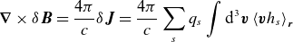 \begin{equation} {\boldsymbol{\nabla }}\times \delta \boldsymbol{B} = \frac {4\pi }{c}\delta \boldsymbol{J} = \frac {4\pi }{c} \sum _s q_{s} \int \textrm {d}^{3} \boldsymbol{v} \left \langle {\boldsymbol{v}}h_{s} \right \rangle _{\boldsymbol{r}} \end{equation}
and the quasineutrality condition
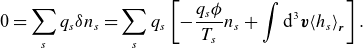 \begin{equation} 0 = \sum _{s} q_{s} \delta n_{s} = \sum _s q_{s} \left [ -\frac {q_{s} \phi }{T_{s}} n_{s} + \int \textrm {d}^{3} \boldsymbol{v}\!\left \langle h_{s} \right \rangle _{\boldsymbol{r}}\right ]. \end{equation}
Equation (2.6) is more commonly split into its parallel and perpendicular parts, as follows:
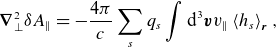 \begin{align} {\boldsymbol{\nabla }}_\perp ^2 \delta A_\parallel &= - \frac {4\pi }{c} \sum _s q_{s} \int \textrm {d}^{3} \boldsymbol{v} v_\parallel \left \langle h_{s} \right \rangle _{\boldsymbol{r}}, \end{align}
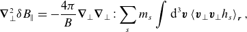 \begin{align} {\boldsymbol{\nabla }}_\perp ^2 \delta B_\parallel & = - \frac {4\pi }{B} {\boldsymbol{\nabla }}_\perp {\boldsymbol{\nabla }}_\perp : \sum _s m_{s} \int \textrm {d}^{3} \boldsymbol{v} \left \langle {\boldsymbol{v}}_\perp {\boldsymbol{v}}_\perp h_{s} \right \rangle _{\boldsymbol{r}}, \\[6pt] \nonumber \end{align}
in which form the latter obviously expresses perpendicular pressure balance.
2.2. Axisymmetric magnetic geometry
We assume that the equilibrium is axisymmetric and that there exist well-defined flux surfaces labelled by the poloidal flux $\psi$
. In this case, it can be shown (see, e.g. Abel et al. Reference Abel, Plunk, Wang, Barnes, Cowley, Dorland and Schekochihin2013) that the plasma equilibrium is, to lowest order in (2.1), a function only of
$\psi$
. In this case, it can be shown (see, e.g. Abel et al. Reference Abel, Plunk, Wang, Barnes, Cowley, Dorland and Schekochihin2013) that the plasma equilibrium is, to lowest order in (2.1), a function only of $\psi$
, i.e.
$\psi$
, i.e. $n_{s} = n_{s}(\psi )$
,
$n_{s} = n_{s}(\psi )$
, $T_{s} = T_{s}(\psi )$
, etc. The equilibrium magnetic field is given by
$T_{s} = T_{s}(\psi )$
, etc. The equilibrium magnetic field is given by $\boldsymbol{B} = {\boldsymbol{\nabla }}\alpha \times {\boldsymbol{\nabla }}\psi$
, where the Clebsch angle is
$\boldsymbol{B} = {\boldsymbol{\nabla }}\alpha \times {\boldsymbol{\nabla }}\psi$
, where the Clebsch angle is $\alpha = \varphi - q(\psi )\theta$
,
$\alpha = \varphi - q(\psi )\theta$
, $\varphi$
is the toroidal angle (the symmetry angle of the axisymmetric equilibrium),
$\varphi$
is the toroidal angle (the symmetry angle of the axisymmetric equilibrium), $\theta$
is the straight-field-line poloidal angle and
$\theta$
is the straight-field-line poloidal angle and $q$
is the safety factor (Kruskal & Kulsrud Reference Kruskal and Kulsrud1958; D’haeseleer et al. Reference D’haeseleer, Hitchon, Callen and Shohet1991). We take
$q$
is the safety factor (Kruskal & Kulsrud Reference Kruskal and Kulsrud1958; D’haeseleer et al. Reference D’haeseleer, Hitchon, Callen and Shohet1991). We take $\theta =0$
to correspond to the outboard midplane of the device.
$\theta =0$
to correspond to the outboard midplane of the device.
In what follows, we shall be working in a field-line-following coordinate system $(x, y, z)$
, where we use
$(x, y, z)$
, where we use $z$
as the coordinate along the equilibrium magnetic field, while
$z$
as the coordinate along the equilibrium magnetic field, while $x \propto \psi$
and
$x \propto \psi$
and $y \propto \alpha$
are the radial and binormal coordinates, respectively, with suitable constant normalisations so that they have units of length. In such a coordinate system,
$y \propto \alpha$
are the radial and binormal coordinates, respectively, with suitable constant normalisations so that they have units of length. In such a coordinate system, ${\boldsymbol{\nabla }} x \times {\boldsymbol{\nabla }} y = \boldsymbol{B} / {B_0}$
, where
${\boldsymbol{\nabla }} x \times {\boldsymbol{\nabla }} y = \boldsymbol{B} / {B_0}$
, where $B_0$
is some constant normalising magnetic field that depends on the choice of
$B_0$
is some constant normalising magnetic field that depends on the choice of $x$
and
$x$
and $y$
. An example of such a choice for
$y$
. An example of such a choice for $x$
,
$x$
, $y$
and
$y$
and $z$
is given in § 2.4.1.
$z$
is given in § 2.4.1.
Finally, let us note that even though the results in this section are derived and presented in axisymmetric geometry, they are readily generalisable to non-axisymmetric geometries.
2.3. Free energy and the GK field invariant
The GK system of equations conserves the free energy
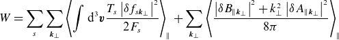
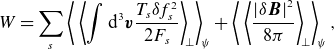 \begin{equation} W = \sum _s \left \langle \,\left \langle {\int \textrm {d}^{3} \boldsymbol{v} \frac {T_{s}\delta f_{s}^2}{2F_{s}}} \right \rangle _{\! \perp } \right \rangle _{\! \psi } + \left \langle \, \left \langle {\frac {\left \rvert {\delta \boldsymbol{B}}\right \rvert ^2}{8\pi }} \right \rangle _{\! \perp } \right \rangle _{\! \psi }, \end{equation}
where $\langle . \rangle _\perp$
and
$\langle . \rangle _\perp$
and $\langle . \rangle _\psi$
denote an intermediate-scale perpendicular average and the flux-surface average, respectively [see (A.1) and (A.6) for their precise definitions]. Physically, their combination is an average over a finite volume around a given flux surface whose radial size is large compared with the fluctuation wavelength
$\langle . \rangle _\psi$
denote an intermediate-scale perpendicular average and the flux-surface average, respectively [see (A.1) and (A.6) for their precise definitions]. Physically, their combination is an average over a finite volume around a given flux surface whose radial size is large compared with the fluctuation wavelength $\sim \rho _{s}$
but small compared with the scale of equilibrium variation
$\sim \rho _{s}$
but small compared with the scale of equilibrium variation $L$
. It can be shown (see Appendix B) that the (collisionless)Footnote
2
time evolution of the free energy is given by
$L$
. It can be shown (see Appendix B) that the (collisionless)Footnote
2
time evolution of the free energy is given by
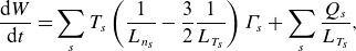 \begin{align} \frac {\textrm {d} {W}}{\textrm {d}{t}} = \sum _s T_{s}\left (\frac {1}{L_{n_{s}}} - \frac {3}{2}\frac {1}{L_{T_{s}}}\right ) \varGamma _s + \sum _s \frac {Q_{s}}{L_{T_{s}}}, \end{align}
where the right-hand side of (2.11) depends on the radial particle and heat (more precisely, energy) fluxes for each species, denoted by $\varGamma _s$
and
$\varGamma _s$
and $Q_s$
, respectively,
$Q_s$
, respectively,
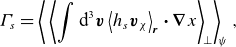 \begin{align} \varGamma _s &= \left \langle \,\left \langle \int \textrm {d}^{3} \boldsymbol{v}\left \langle h_{s} \boldsymbol{v}_{\chi } \right \rangle _{\boldsymbol{r}} \boldsymbol{\cdot } {\boldsymbol{\nabla }} x\right \rangle _{\! \perp }\right \rangle _{\! \psi }, \end{align}
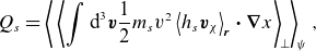 \begin{align} Q_{s} &= \left \langle \,\left \langle {\int \textrm {d}^{3} \boldsymbol{v}\frac {1}{2}m_{s} v^2\left \langle h_{s} \boldsymbol{v}_{\chi } \right \rangle _{\boldsymbol{r}} \boldsymbol{\cdot } {\boldsymbol{\nabla }} x} \right \rangle _{\! \perp } \right \rangle _{\! \psi } , \\[6pt] \nonumber \end{align}
and the density and temperature gradient length scales are defined as
 \begin{equation} \frac {1}{L_{n_{s}}} \equiv -\frac {\textrm {d}\,{\ln n_{s}}}{\textrm {d}{x}}, \quad \frac {1}{L_{T_{s}}} \equiv -\frac {\textrm {d}\,{\ln T_{s}}}{\textrm {d}{x}}. \end{equation}
Note that (2.11) is a local conservation law valid at any given flux surface. Thus, to lowest order in (2.1), free energy is injected and dissipated at every flux surface separately, i.e. there is no overall transport of free energy across flux surfaces (Abel et al. Reference Abel, Plunk, Wang, Barnes, Cowley, Dorland and Schekochihin2013). The right-hand side of (2.11) shows that free energy is injected into fluctuations by the density and heat fluxes along the gradients of the plasma equilibrium. The magnetic drifts are absent from (2.11). This is the well-known result that GK fluctuations cannot directly access the energy stored in the equilibrium magnetic field (Abel et al. Reference Abel, Plunk, Wang, Barnes, Cowley, Dorland and Schekochihin2013). Thus, even though the magnetic drifts are, by definition, required for any curvature-driven instability, we cannot use the conservation of free energy by itself to determine their role in the said instabilities.
To elucidate the role of the magnetic drifts, we construct another nonlinearly conserved quantity, which we call the GK field invariant, defined as
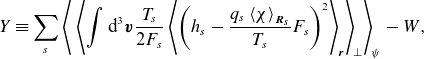 \begin{equation} Y \equiv \sum _s \left \langle \,\left \langle {\int \textrm {d}^{3} \boldsymbol{v} \frac {T_{s}}{2F_{s}} \left \langle \left (h_{s} - \frac {q_{s}\left \langle \chi \right \rangle _{{\boldsymbol{R}_{s}}}}{T_{s}}F_{s}\right )^2 \right \rangle _{\boldsymbol{r}}} \right \rangle _{\! \perp } \right \rangle _{\! \psi } - W, \end{equation}
where $\left \langle . \right \rangle _{\boldsymbol{r}}$
is the standard gyroaverage at fixed
$\left \langle . \right \rangle _{\boldsymbol{r}}$
is the standard gyroaverage at fixed $\boldsymbol{r}$
. The field invariant can be shown to satisfy (see Appendix B.4)
$\boldsymbol{r}$
. The field invariant can be shown to satisfy (see Appendix B.4)
 \begin{equation} \frac {\textrm {d}{Y}}{\textrm {d}{t}} = \sum _s \left \langle \,\left \langle {\int \textrm {d}^{3} \boldsymbol{v} \left \langle q_{s}\left \langle \chi \right \rangle _{{\boldsymbol{R}_{s}}}v_\parallel {{\hat {\boldsymbol{b}}}}\boldsymbol{\cdot }{\boldsymbol{\nabla }}h_{s} + q_{s} \left \langle \chi \right \rangle _{{\boldsymbol{R}_{s}}} \boldsymbol{v}_{\text{d}s} \boldsymbol{\cdot } {\boldsymbol{\nabla }}_\perp h_{s} \right \rangle _{\boldsymbol{r}}} \right \rangle _{\! \perp } \right \rangle _{\! \psi }. \end{equation}
It is related to the general two-dimensional invariants of GK (Schekochihin et al. Reference Schekochihin, Cowley, Dorland, Hammett, Howes, Quataert and Tatsuno2009; Plunk et al. Reference Plunk, Cowley, Schekochihin and Tatsuno2010) and can be thought of as a generalisation of the so-called ‘electrostatic invariant’ (Schekochihin et al. Reference Schekochihin, Cowley, Dorland, Hammett, Howes, Quataert and Tatsuno2009; Plunk et al. Reference Plunk, Cowley, Schekochihin and Tatsuno2010; Helander et al. Reference Helander, Proll and Plunk2013; Plunk & Helander Reference Plunk and Helander2023). Note that even though the nonlinear terms do not contribute to the evolution of $Y$
, it still evolves collisionlessly in a uniform plasma and a uniform magnetic field due to the presence of the parallel streaming term on the right-hand side of (2.16). In contrast,
$Y$
, it still evolves collisionlessly in a uniform plasma and a uniform magnetic field due to the presence of the parallel streaming term on the right-hand side of (2.16). In contrast, $W$
is a ‘true’ invariant for which
$W$
is a ‘true’ invariant for which $\textrm {d} W / \textrm {d} t$
vanishes exactly in the absence of equilibrium gradients and collisions. Thus, the relevance of the field invariant to the study of nonlinear turbulent saturation is likely limited to two-dimensional or nearly two-dimensional situations wherein the parallel-streaming term can be ignored (Plunk et al. Reference Plunk, Cowley, Schekochihin and Tatsuno2010).
$\textrm {d} W / \textrm {d} t$
vanishes exactly in the absence of equilibrium gradients and collisions. Thus, the relevance of the field invariant to the study of nonlinear turbulent saturation is likely limited to two-dimensional or nearly two-dimensional situations wherein the parallel-streaming term can be ignored (Plunk et al. Reference Plunk, Cowley, Schekochihin and Tatsuno2010).
Nevertheless, the field invariant can be a powerful tool in the study of linear instabilities.Footnote
3
The (collisionless) time evolution of $Y$
, given by (2.16), contains two contributions: one from parallel streaming and one from the magnetic drifts. We will shortly argue that the former is the physically important source of
$Y$
, given by (2.16), contains two contributions: one from parallel streaming and one from the magnetic drifts. We will shortly argue that the former is the physically important source of $Y$
for slab instabilities. The latter will turn out to determine the instability of curvature-driven modes. In Appendix B.4, we show that it can be written as
$Y$
for slab instabilities. The latter will turn out to determine the instability of curvature-driven modes. In Appendix B.4, we show that it can be written as
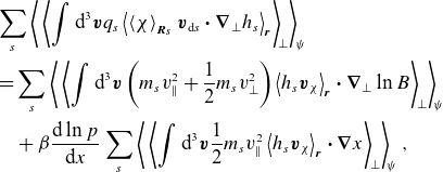 \begin{align} &\sum _s \left \langle \,\left \langle {\int \textrm {d}^{3} \boldsymbol{v} q_{s} \left \langle \left \langle \chi \right \rangle _{{\boldsymbol{R}_{s}}} \boldsymbol{v}_{\text{d}s}\boldsymbol{\cdot }{\boldsymbol{\nabla }}_\perp h_{s} \right \rangle _{\boldsymbol{r}}} \right \rangle _{\! \perp } \right \rangle _{\! \psi } \nonumber \\ & = \sum _s \left \langle \,\left \langle {\int \textrm {d}^{3} \boldsymbol{v} \left (m_{s}v_\parallel ^2 + \frac {1}{2}m_{s}v_\perp ^2 \right ) \left \langle h_{s} \boldsymbol{v}_{\chi } \right \rangle _{\boldsymbol{r}}\boldsymbol{\cdot } {\boldsymbol{\nabla }}_\perp \ln B} \right \rangle _{\! \perp } \right \rangle _{\! \psi } \nonumber \\ &\quad + \beta \frac {\textrm {d}\,{\ln p}}{\textrm{d}{x}} \sum _{s} \left \langle \, \left \langle \int \textrm {d}^{3} \boldsymbol{v} \frac {1}{2} m_{s} v_{\parallel}^{2} \left \langle h_{s} \boldsymbol{v}_{\chi } \right \rangle _{\boldsymbol{r}} \boldsymbol{\cdot } {\boldsymbol{\nabla }} x \right \rangle _{\! \perp } \right \rangle _{\! \psi }, \end{align}
where $\beta = 8\pi p / B^2$
is the plasma beta and
$\beta = 8\pi p / B^2$
is the plasma beta and $p = \sum _s n_{s}T_{s}$
is the equilibrium pressure. Equation (2.17) suggests that the injection of
$p = \sum _s n_{s}T_{s}$
is the equilibrium pressure. Equation (2.17) suggests that the injection of $Y$
due to the magnetic drifts has a form very similar to that of
$Y$
due to the magnetic drifts has a form very similar to that of $W$
, viz. it is proportional to the turbulent heat flux across the equilibrium magnetic field, but also depends directly on the gradient of the magnetic field. As the vector
$W$
, viz. it is proportional to the turbulent heat flux across the equilibrium magnetic field, but also depends directly on the gradient of the magnetic field. As the vector ${\boldsymbol{\nabla }}_\perp \ln B$
is, in general, not aligned with
${\boldsymbol{\nabla }}_\perp \ln B$
is, in general, not aligned with ${\boldsymbol{\nabla }} x$
, it is not straightforward to relate the injection terms of
${\boldsymbol{\nabla }} x$
, it is not straightforward to relate the injection terms of $W$
and
$W$
and $Y$
, i.e. the right-hand sides of (2.11) and (2.17). In § 2.4, we deal with this by making some additional assumptions about the nature of the instabilities and the magnetic geometry.
$Y$
, i.e. the right-hand sides of (2.11) and (2.17). In § 2.4, we deal with this by making some additional assumptions about the nature of the instabilities and the magnetic geometry.
2.3.1. Local limit
To make further progress, we restrict ourselves to what is commonly known as the ‘local $\delta f$
gyrokinetics’. Here ‘local’ means that we are integrating (2.4) in a domain of perpendicular size that is infinitesimal in comparison with the length scales associated with the plasma equilibrium
$\delta f$
gyrokinetics’. Here ‘local’ means that we are integrating (2.4) in a domain of perpendicular size that is infinitesimal in comparison with the length scales associated with the plasma equilibrium $F_{s}$
and the equilibrium magnetic field
$F_{s}$
and the equilibrium magnetic field $\boldsymbol{B}$
, and so the (perpendicular) gradients associated with the equilibrium are taken to be constant; ‘
$\boldsymbol{B}$
, and so the (perpendicular) gradients associated with the equilibrium are taken to be constant; ‘ $\delta f$
’ means that we only consider the evolution of small-amplitude fluctuations over times that are short compared with the transport time scale (over which the equilibrium evolves), with the equilibrium therefore assumed constant in time.
$\delta f$
’ means that we only consider the evolution of small-amplitude fluctuations over times that are short compared with the transport time scale (over which the equilibrium evolves), with the equilibrium therefore assumed constant in time.
In the local approximation, any fluctuating quantity $g({\boldsymbol{r}})$
can be written as
$g({\boldsymbol{r}})$
can be written as
 \begin{equation} g({\boldsymbol{r}}) = \sum _{{\boldsymbol{k}}_\perp } g_{{\boldsymbol{k}}_\perp }(z) \textrm {e}^{\textrm {i} k_x x + \textrm {i} k_y y}, \end{equation}
where the field-line-following coordinate system $(x, y, z)$
is defined at the end of § 2.2. Equation (2.18) can be thought of as an ensemble of modes in the ballooning representation (Connor, Hastie & Taylor Reference Connor, Hastie and Taylor1978). Alternatively, and perhaps more practically for numerical simulations, fluctuations have the form (2.18) when solving (2.4) in a field-line-following flux tube (Beer, Cowley & Hammett Reference Beer, Cowley and Hammett1995) and imposing periodic boundary conditions in the plane perpendicular to the magnetic field.Footnote
4
Further details on the validity of (2.18) and the relationship between the ballooning transformation and the local GK formulation can be found in Beer et al. (Reference Beer, Cowley and Hammett1995) and Appendix A. For the purposes of the following discussion, we consider modes in a periodic flux tube with an infinite extent along the field lines. In this case, the free energy (2.10) and field invariant (2.15) can be expressed as
$(x, y, z)$
is defined at the end of § 2.2. Equation (2.18) can be thought of as an ensemble of modes in the ballooning representation (Connor, Hastie & Taylor Reference Connor, Hastie and Taylor1978). Alternatively, and perhaps more practically for numerical simulations, fluctuations have the form (2.18) when solving (2.4) in a field-line-following flux tube (Beer, Cowley & Hammett Reference Beer, Cowley and Hammett1995) and imposing periodic boundary conditions in the plane perpendicular to the magnetic field.Footnote
4
Further details on the validity of (2.18) and the relationship between the ballooning transformation and the local GK formulation can be found in Beer et al. (Reference Beer, Cowley and Hammett1995) and Appendix A. For the purposes of the following discussion, we consider modes in a periodic flux tube with an infinite extent along the field lines. In this case, the free energy (2.10) and field invariant (2.15) can be expressed as
 \begin{equation} W = \sum _s \sum _{{\boldsymbol{k}}_\perp } \left \langle \int \textrm {d}^{3} \boldsymbol{v} \frac {T_{s}\left \rvert {\delta {f}_{{s}{{\boldsymbol{k}}_\perp }}}\right \rvert ^2}{2F_{s}}\right \rangle _ \parallel + \sum _{{\boldsymbol{k}}_\perp } \left \langle \frac {\left \rvert {\delta {B}_{\parallel {{\boldsymbol{k}}_\perp }}}\right \rvert ^2 + k_\perp ^2\left \rvert {\delta {A}_{\parallel {{\boldsymbol{k}}_\perp }}}\right \rvert ^2}{8\pi }\right \rangle _ \parallel \end{equation}
and
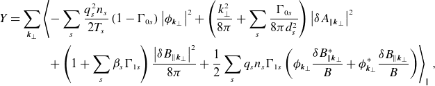 \begin{align} Y = \sum _{{\boldsymbol{k}}_\perp } & \left \langle -\sum _{s} \frac {q_{s}^2n_{s}}{2T_{s}}\left (1-\mathrm{\Gamma }_{0s}\right )\left \rvert {{\phi }_{{\boldsymbol{k}}_\perp }}\right \rvert ^2 + \left (\frac {k_\perp ^2}{8\pi } + \sum _s \frac {\mathrm{\Gamma }_{0s}}{8\pi d_{s}^2}\right )\left \rvert {\delta {A}_{\parallel {{\boldsymbol{k}}_\perp }}}\right \rvert ^2 \right .\nonumber \\ &\quad\!\!\!\left .+ \left (1 + \sum _s \beta _{s}\mathrm{\Gamma }_{1s}\right )\frac {\left \rvert {\delta {B}_{\parallel {{\boldsymbol{k}}_\perp }}}\right \rvert ^2}{8\pi } + \frac {1}{2}\sum _sq_{s}n_{s}\mathrm{\Gamma }_{1s}\left ({\phi }_{{\boldsymbol{k}}_\perp }\frac {\delta {B}_{\parallel {{\boldsymbol{k}}_\perp }}^*}{B} + {\phi }_{{\boldsymbol{k}}_\perp }^*\frac {\delta {B}_{\parallel {{\boldsymbol{k}}_\perp }}}{B}\right ) \right \rangle _\parallel , \end{align}
respectively, where $\langle .\rangle _\parallel$
denotes the parallel average [defined in (A.15)]. It is defined in such a way that the combination of the sum over
$\langle .\rangle _\parallel$
denotes the parallel average [defined in (A.15)]. It is defined in such a way that the combination of the sum over ${\boldsymbol{k}}_\perp$
and the parallel average is equivalent to the combination of the perpendicular and flux-surface average (see Appendix A.1 for details). In (2.20),
${\boldsymbol{k}}_\perp$
and the parallel average is equivalent to the combination of the perpendicular and flux-surface average (see Appendix A.1 for details). In (2.20), $d_{s} = \rho _{s}/\sqrt {\beta _{s}}$
and
$d_{s} = \rho _{s}/\sqrt {\beta _{s}}$
and $\beta _{s} = 8\pi n_{s}T_{s}/B^2$
are the skin depth (or inertial length) and plasma beta of species
$\beta _{s} = 8\pi n_{s}T_{s}/B^2$
are the skin depth (or inertial length) and plasma beta of species $s$
, respectively, and
$s$
, respectively, and
 \begin{align} \mathrm{\Gamma }_{0s} = \textrm {I}_0(\alpha _s)\textrm {e}^{-\alpha _s}, \quad \mathrm{\Gamma }_{1s} = \left [\textrm {I}_0(\alpha _s) - \textrm {I}_1(\alpha _s)\right ] \textrm {e}^{-\alpha _s}, \end{align}
where $\alpha _s = k_\perp ^2\rho _{s}^2/2$
,
$\alpha _s = k_\perp ^2\rho _{s}^2/2$
, $k_\perp ^2 = (k_x {\boldsymbol{\nabla }} x + k_y {\boldsymbol{\nabla }} y)^2$
, and
$k_\perp ^2 = (k_x {\boldsymbol{\nabla }} x + k_y {\boldsymbol{\nabla }} y)^2$
, and $\textrm {I}_0$
and
$\textrm {I}_0$
and $\textrm {I}_1$
are the modified Bessel functions of the first kind.
$\textrm {I}_1$
are the modified Bessel functions of the first kind.
When written as (2.19) and (2.20), it is evident that the field invariant $Y$
differs from the free energy
$Y$
differs from the free energy $W$
in two crucial ways. First, the distribution function
$W$
in two crucial ways. First, the distribution function $\delta f_{s}$
does not enter explicitly into the former, which contains contributions only from the electromagnetic fields, justifying the name ‘field’ invariant. Secondly, unlike the free energy, which is always positive,
$\delta f_{s}$
does not enter explicitly into the former, which contains contributions only from the electromagnetic fields, justifying the name ‘field’ invariant. Secondly, unlike the free energy, which is always positive, $Y$
is not sign definite, as is evident in (2.20). Since
$Y$
is not sign definite, as is evident in (2.20). Since $1 - \mathrm{\Gamma }_{0s}$
is strictly positive, the electrostatic part of the invariant, viz. the part proportional to
$1 - \mathrm{\Gamma }_{0s}$
is strictly positive, the electrostatic part of the invariant, viz. the part proportional to $\rvert {\phi }_{{\boldsymbol{k}}_\perp }\rvert ^2$
in (2.20), is negative definite, while including electromagnetic effects makes
$\rvert {\phi }_{{\boldsymbol{k}}_\perp }\rvert ^2$
in (2.20), is negative definite, while including electromagnetic effects makes $Y$
sign-indefinite. In particular,
$Y$
sign-indefinite. In particular, $Y$
can be positive only for large enough
$Y$
can be positive only for large enough $\delta {A}_{\parallel {{\boldsymbol{k}}_\perp }}$
and/or
$\delta {A}_{\parallel {{\boldsymbol{k}}_\perp }}$
and/or $\delta {B}_{\parallel {{\boldsymbol{k}}_\perp }}$
. These observations will be crucial for the arguments presented in § 2.4.
$\delta {B}_{\parallel {{\boldsymbol{k}}_\perp }}$
. These observations will be crucial for the arguments presented in § 2.4.
In general, the physical meaning of $Y$
is not transparent. However, in certain limits, it can be related to other, better-known conserved quantities. For instance, in the electrostatic limit, viz.
$Y$
is not transparent. However, in certain limits, it can be related to other, better-known conserved quantities. For instance, in the electrostatic limit, viz. $\delta {A}_{\parallel {{\boldsymbol{k}}_\perp }} = 0$
and
$\delta {A}_{\parallel {{\boldsymbol{k}}_\perp }} = 0$
and $\delta {B}_{\parallel {{\boldsymbol{k}}_\perp }} = 0$
, (2.20) becomes the usual electrostatic invariant (Schekochihin et al. Reference Schekochihin, Cowley, Dorland, Hammett, Howes, Quataert and Tatsuno2009; Plunk et al. Reference Plunk, Cowley, Schekochihin and Tatsuno2010; Helander et al. Reference Helander, Proll and Plunk2013)
$\delta {B}_{\parallel {{\boldsymbol{k}}_\perp }} = 0$
, (2.20) becomes the usual electrostatic invariant (Schekochihin et al. Reference Schekochihin, Cowley, Dorland, Hammett, Howes, Quataert and Tatsuno2009; Plunk et al. Reference Plunk, Cowley, Schekochihin and Tatsuno2010; Helander et al. Reference Helander, Proll and Plunk2013)
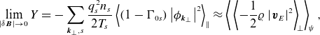 \begin{equation} \lim _{\rvert \delta \boldsymbol{B}\rvert \to 0} Y = -\sum _{{{\boldsymbol{k}}_\perp }, s} \frac {q_{s}^2n_{s}}{2T_{s}}\left \langle \left (1-\mathrm{\Gamma }_{0s}\right )\left \rvert {{\phi }_{{\boldsymbol{k}}_\perp }}\right \rvert ^2\right \rangle _ \parallel \approx \left \langle \,\left \langle {-\frac {1}{2}\varrho \left \rvert {\boldsymbol{v}_{E}}\right \rvert ^2} \right \rangle _{\! \perp } \right \rangle _{\! \psi }, \end{equation}
where the last (approximate) equality holds in the long-wavelength limit ( $k_\perp \rho _{s} \ll 1$
for all species
$k_\perp \rho _{s} \ll 1$
for all species $s$
). In this limit,
$s$
). In this limit, $Y$
is simply (the negative of) the total kinetic energy associated with the
$Y$
is simply (the negative of) the total kinetic energy associated with the $\boldsymbol{E}\times \boldsymbol{B}$
velocity of the particles
$\boldsymbol{E}\times \boldsymbol{B}$
velocity of the particles $\boldsymbol{v}_{E} = (c/B){{\hat {\boldsymbol{b}}}}\times {\boldsymbol{\nabla }}\phi$
and its total density
$\boldsymbol{v}_{E} = (c/B){{\hat {\boldsymbol{b}}}}\times {\boldsymbol{\nabla }}\phi$
and its total density $\varrho \equiv \sum _s m_{s}n_{s}$
. Restoring the contributions from the magnetic fluctuations, we find
$\varrho \equiv \sum _s m_{s}n_{s}$
. Restoring the contributions from the magnetic fluctuations, we find
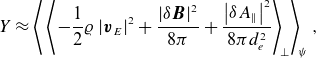 \begin{equation} Y \approx \left \langle \,\left \langle {-\frac {1}{2}\varrho \left \rvert {\boldsymbol{v}_{E}}\right \rvert ^2 + \frac {\left \rvert {\delta \boldsymbol{B}}\right \rvert ^2}{8\pi } + \frac {\left \rvert {\delta A_\parallel }\right \rvert ^2}{8\pi d_{e}^2}} \right \rangle _{\! \perp } \right \rangle _{\! \psi }, \end{equation}
where we have assumed a ‘typical’ plasma of multiple ion species and one electron species of significantly lower mass. The last term in (2.23), which dominates when $k_\perp d_{e} \ll 1$
, can be recognised as anastrophy (or ‘
$k_\perp d_{e} \ll 1$
, can be recognised as anastrophy (or ‘ $A_\parallel ^2$
-stuff’) – a well-known two-dimensional invariant of MHD (Fyfe & Montgomery Reference Fyfe and Montgomery1976; Pouquet Reference Pouquet1978; Schekochihin Reference Schekochihin2022). Thus, in the MHD limit, the field invariant can be though of as the anastrophy with an additional correction due to kinetic physics.
$A_\parallel ^2$
-stuff’) – a well-known two-dimensional invariant of MHD (Fyfe & Montgomery Reference Fyfe and Montgomery1976; Pouquet Reference Pouquet1978; Schekochihin Reference Schekochihin2022). Thus, in the MHD limit, the field invariant can be though of as the anastrophy with an additional correction due to kinetic physics.
Using (2.18), the free-energy conservation law (2.11) can be written as
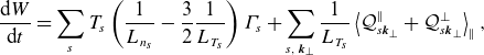 \begin{align} \frac {\textrm {d} {W}}{\textrm {d}{t}} &= \sum _s T_{s}\left (\frac {1}{L_{n_{s}}} - \frac {3}{2}\frac {1}{L_{T_{s}}}\right ) \varGamma _s + \sum _{s,\:{{\boldsymbol{k}}_\perp }} \frac {1}{L_{T_{s}}} \left \langle \mathcal{Q}^{\parallel }_{s{{\boldsymbol{k}}_\perp }} + \mathcal{Q}^{\perp }_{s{{\boldsymbol{k}}_\perp }}\right \rangle _ \parallel , \end{align}
where we have defined the local (in $z$
) radial fluxes of energy associated with parallel and perpendicular particle motion,
$z$
) radial fluxes of energy associated with parallel and perpendicular particle motion,
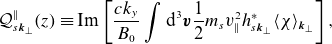 \begin{align} \mathcal{Q}^{\parallel }_{s{{\boldsymbol{k}}_\perp }}(z) &\equiv \text{Im} \left [\frac {c k_y}{{B_0}} \int \textrm {d}^{3} \boldsymbol{v} \frac {1}{2}m_{s}v_\parallel ^2 {h}_{{s}{{\boldsymbol{k}}_\perp }}^* \langle \chi \rangle _{{\boldsymbol{k}}_\perp }\right ], \end{align}
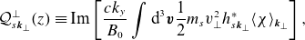 \begin{align} \mathcal{Q}^{\perp }_{s{{\boldsymbol{k}}_\perp }}(z) &\equiv \text{Im} \left [\frac {c k_y}{{B_0}} \int \textrm {d}^{3} \boldsymbol{v} \frac {1}{2}m_{s}v_\perp ^2 {h}_{{s}{{\boldsymbol{k}}_\perp }}^*\langle \chi \rangle _{{\boldsymbol{k}}_\perp }\right ], \\[6pt] \nonumber \end{align}
where $\langle \chi \rangle _{{\boldsymbol{k}}_\perp }$
is the Fourier-transformed gyroaveraged GK potential [see (B.18)]. These fluxes are related to the total heat flux by
$\langle \chi \rangle _{{\boldsymbol{k}}_\perp }$
is the Fourier-transformed gyroaveraged GK potential [see (B.18)]. These fluxes are related to the total heat flux by $Q_{s} = \sum _{{\boldsymbol{k}}_\perp }\langle \mathcal{Q}^{\parallel }_{s{{\boldsymbol{k}}_\perp }} + \mathcal{Q}^{\perp }_{s{{\boldsymbol{k}}_\perp }}\rangle _\parallel$
.
$Q_{s} = \sum _{{\boldsymbol{k}}_\perp }\langle \mathcal{Q}^{\parallel }_{s{{\boldsymbol{k}}_\perp }} + \mathcal{Q}^{\perp }_{s{{\boldsymbol{k}}_\perp }}\rangle _\parallel$
.
Similarly, for the field invariant, we find
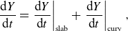 \begin{align} \frac {\textrm {d}{Y}}{\textrm {d}{t}} &= \left .\frac {\textrm {d}{Y}}{\textrm {d}{t}}\right \rvert _{\text{slab}} + \left .\frac {\textrm {d}{Y}}{\textrm {d}{t}}\right \rvert _{\text{curv}}, \end{align}
where we have separated the ‘slab’ contribution to (2.16) arising from the parallel streaming,
 \begin{equation} \left .\frac {\textrm {d}{Y}}{\textrm {d}{t}}\right \rvert _{\text{slab}} = \sum _{s,\: {{\boldsymbol{k}}_\perp }}\left \langle \int \textrm {d}^{3} \boldsymbol{v}\,q_{s}v_\parallel \langle \chi \rangle _{{\boldsymbol{k}}_\perp } {{\hat {\boldsymbol{b}}}}\boldsymbol{\cdot } {\boldsymbol{\nabla }} {h}_{{s}{{\boldsymbol{k}}_\perp }}^*\right \rangle _ \parallel , \end{equation}
and the ‘curvature’ one due to the magnetic drifts,
 \begin{equation} \left .\frac {\textrm {d}{Y}}{\textrm {d}{t}}\right \rvert _{\text{curv}} = 2\sum _{{\boldsymbol{k}}_\perp }\left \langle \mathcal{C}_{{\boldsymbol{k}}_\perp } \mathcal{Q}^{\parallel }_{{\boldsymbol{k}}_\perp }\right \rangle _ \parallel . \end{equation}
Here the local magnetic curvature is defined as
 \begin{equation} \mathcal{C}_{{\boldsymbol{k}}_\perp }(z) \equiv (2+a_{{\boldsymbol{k}}_\perp })\frac {{B_0}}{B} ({{\hat {\boldsymbol{b}}}}\times {\boldsymbol{\nabla }}_\perp \ln B) \boldsymbol{\cdot } \left ( {\boldsymbol{\nabla }} y + \frac {k_x}{k_y}{\boldsymbol{\nabla }} x\right ) + \frac {\beta }{2}\frac {\textrm {d}\,{\ln p}}{\textrm {d}{x}}, \end{equation}
where $a_{{\boldsymbol{k}}_\perp }(z) \equiv (\mathcal{Q}^{\perp }_{{\boldsymbol{k}}_\perp } - 2\mathcal{Q}^{\parallel }_{{\boldsymbol{k}}_\perp })/2\mathcal{Q}^{\parallel }_{{\boldsymbol{k}}_\perp }$
is the heat-flux anisotropy parameter, defined as the ratio of the total parallel
$a_{{\boldsymbol{k}}_\perp }(z) \equiv (\mathcal{Q}^{\perp }_{{\boldsymbol{k}}_\perp } - 2\mathcal{Q}^{\parallel }_{{\boldsymbol{k}}_\perp })/2\mathcal{Q}^{\parallel }_{{\boldsymbol{k}}_\perp }$
is the heat-flux anisotropy parameter, defined as the ratio of the total parallel $\mathcal{Q}^{\parallel }_{{\boldsymbol{k}}_\perp } \equiv \sum _s \mathcal{Q}^{\parallel }_{s{{\boldsymbol{k}}_\perp }}$
and perpendicular
$\mathcal{Q}^{\parallel }_{{\boldsymbol{k}}_\perp } \equiv \sum _s \mathcal{Q}^{\parallel }_{s{{\boldsymbol{k}}_\perp }}$
and perpendicular $\mathcal{Q}^{\perp }_{{\boldsymbol{k}}_\perp } \equiv \sum _s \mathcal{Q}^{\perp }_{s{{\boldsymbol{k}}_\perp }}$
heat fluxes. For isotropic fluctuations, in particular,
$\mathcal{Q}^{\perp }_{{\boldsymbol{k}}_\perp } \equiv \sum _s \mathcal{Q}^{\perp }_{s{{\boldsymbol{k}}_\perp }}$
heat fluxes. For isotropic fluctuations, in particular, $a_{{\boldsymbol{k}}_\perp } = 0$
.
$a_{{\boldsymbol{k}}_\perp } = 0$
.
When considering a single mode, the contributions to the right-hand side of (2.27) provide a natural distinction between slab and curvature-driven dynamics. By definition, the former are those that survive in a straight uniform magnetic field, where the magnetic drifts vanish, and so does (2.29). Thus, the parallel-streaming term (2.28) is the physically important source of $Y$
for slab instabilities even if both (2.28) and (2.29) happen to be nonzero in the presence of magnetic drifts. In contrast, curvature-driven modes are those whose dominant
$Y$
for slab instabilities even if both (2.28) and (2.29) happen to be nonzero in the presence of magnetic drifts. In contrast, curvature-driven modes are those whose dominant $Y$
-injection term is (2.29). These modes are destabilised by the combination of the thermal-equilibrium gradients and the magnetic geometry.
$Y$
-injection term is (2.29). These modes are destabilised by the combination of the thermal-equilibrium gradients and the magnetic geometry.
2.4. Curvature-driven temperature-gradient instabilities
Let us consider a single unstable mode, i.e. a fluctuation with given $k_x$
and
$k_x$
and $k_y$
, with amplitude proportional to
$k_y$
, with amplitude proportional to $\textrm {e}^{-\textrm {i}\omega t}$
, where
$\textrm {e}^{-\textrm {i}\omega t}$
, where $\text{Im}(\omega ) \gt 0$
is the growth rate. As both
$\text{Im}(\omega ) \gt 0$
is the growth rate. As both $W$
and
$W$
and $Y$
are quadratic in the fluctuation amplitude, this implies that the free energy and the field invariant associated with a single mode satisfy
$Y$
are quadratic in the fluctuation amplitude, this implies that the free energy and the field invariant associated with a single mode satisfy
 \begin{equation} \frac {\textrm {d} {W}}{\textrm {d}{t}} = 2\text{Im}(\omega ) W, \quad \frac {\textrm {d}{Y}}{\textrm {d}{t}} = 2\text{Im}(\omega ) Y. \end{equation}
We now make three simplifying assumptions.
-
(i) We assume that the injection of free energy of the mode is dominated by the heat rather than the particle fluxes, so we can ignore the latter in (2.24). We refer to such fluctuations as ‘temperature-gradient’ modes. While this might seem very restrictive, there are, in fact, many instabilities that satisfy this condition. One example are modes for which there is a main species $s$
, with all other species
$s'$
assumed adiabatic (or ‘modified’ adiabatic in the case of ion-scale turbulence: see Hammett et al. Reference Hammett, Beer, Dorland, Cowley and Smith1993). For such instabilities, the non-adiabatic distribution functions
$h_{s'}$
for the species
$s'\neq s$
are small, in which case the particle flux vanishes.
$s$
, with all other species
$s'$
assumed adiabatic (or ‘modified’ adiabatic in the case of ion-scale turbulence: see Hammett et al. Reference Hammett, Beer, Dorland, Cowley and Smith1993). For such instabilities, the non-adiabatic distribution functions
$h_{s'}$
for the species
$s'\neq s$
are small, in which case the particle flux vanishes. -
(ii) We assume that the unstable mode is curvature-driven and so the slab injection term in (2.27) can be ignored. The ratio of (2.28) and (2.29) for a curvature-driven mode can be estimated as
(2.32)where
\begin{align} \frac {\textrm {d} Y / \textrm {d} t \vert _{\text{slab}}}{\textrm {d} Y / \textrm {d} t \vert _{\text{curv}}} \sim \frac {k_\parallel v_{\text{th}{s}}}{\omega _{\text{d}s}}, \end{align}
$\omega _{\text{d}s} = {{\boldsymbol{k}}_\perp } \boldsymbol{\cdot } \boldsymbol{v}_{\text{d}s}$
is the magnetic-drift frequency and
$k_\parallel \sim ({{\hat {\boldsymbol{b}}}} \boldsymbol{\cdot } {\boldsymbol{\nabla }} h_{s}) / h_{s}$
is the effective parallel wavenumber. Therefore, the assumption of neglecting (2.28) in favour of (2.29) in (2.27) can be made asymptotic in the limit
$k_\parallel v_{\text{th}{s}} \ll \omega _{\text{d}s}$
, i.e. in the limit of long parallel length scales.Footnote
5
-
(iii) We assume that the heat flux is dominated by a single, ‘main’ species
$s$
. We make this choice purely for the purposes of simplifying the discussion below. Our arguments hold even if multiple species contribute to the injection of
$W$
and
$Y$
if the temperature gradients of the species that contribute the majority of the heat flux are aligned.


Without loss of generality, we can choose the flux-surface label $x$
so that
$x$
so that $L_{T_{s}} \gt 0$
. Therefore, due to (2.31) and the positive-definiteness of
$L_{T_{s}} \gt 0$
. Therefore, due to (2.31) and the positive-definiteness of $W$
, the heat flux
$W$
, the heat flux $Q_{s} = \langle \mathcal{Q}^{\parallel }_{s{{\boldsymbol{k}}_\perp }} + \mathcal{Q}^{\perp }_{s{{\boldsymbol{k}}_\perp }}\rangle _\parallel$
appearing in (2.24) must be positive for any unstable mode with
$Q_{s} = \langle \mathcal{Q}^{\parallel }_{s{{\boldsymbol{k}}_\perp }} + \mathcal{Q}^{\perp }_{s{{\boldsymbol{k}}_\perp }}\rangle _\parallel$
appearing in (2.24) must be positive for any unstable mode with $\text{Im}\:\omega \gt 0$
. This is intuitively clear: temperature-gradient-driven instabilities predominantly transport heat down the temperature gradient, from the hot to the cold regions of the equilibrium.
$\text{Im}\:\omega \gt 0$
. This is intuitively clear: temperature-gradient-driven instabilities predominantly transport heat down the temperature gradient, from the hot to the cold regions of the equilibrium.
Assuming that $\mathcal{Q}^{\parallel }_{s{{\boldsymbol{k}}_\perp }} \sim \mathcal{Q}^{\perp }_{s{{\boldsymbol{k}}_\perp }}$
(or at least that they have the same sign), (2.27), (2.29) and (2.31) imply thatFootnote
6
$\mathcal{Q}^{\parallel }_{s{{\boldsymbol{k}}_\perp }} \sim \mathcal{Q}^{\perp }_{s{{\boldsymbol{k}}_\perp }}$
(or at least that they have the same sign), (2.27), (2.29) and (2.31) imply thatFootnote
6
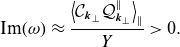 \begin{align} \text{Im}(\omega ) \approx \frac {\left \langle \mathcal{C}_{{\boldsymbol{k}}_\perp } \mathcal{Q}^{\parallel }_{{\boldsymbol{k}}_\perp }\right \rangle _ \parallel }{Y} \gt 0. \end{align}
Since the heat flux $\mathcal{Q}^{\parallel }_{{\boldsymbol{k}}_\perp }(z)$
is positive and the local magnetic curvature
$\mathcal{Q}^{\parallel }_{{\boldsymbol{k}}_\perp }(z)$
is positive and the local magnetic curvature $\mathcal{C}_{{\boldsymbol{k}}_\perp }(z)$
changes sign along the field line (we provide a simple example of this in § 2.4.1), in order for (2.33) to be satisfied, the heat flux must be larger at those locations along the field line where
$\mathcal{C}_{{\boldsymbol{k}}_\perp }(z)$
changes sign along the field line (we provide a simple example of this in § 2.4.1), in order for (2.33) to be satisfied, the heat flux must be larger at those locations along the field line where $\mathcal{C}_{{\boldsymbol{k}}_\perp }(z)$
has the same sign as
$\mathcal{C}_{{\boldsymbol{k}}_\perp }(z)$
has the same sign as $Y$
. Therefore, if
$Y$
. Therefore, if $Y \gt 0$
, the heat flux, and thus the mode amplitude, must peak at the places where
$Y \gt 0$
, the heat flux, and thus the mode amplitude, must peak at the places where $\mathcal{C}_{{\boldsymbol{k}}_\perp }(z) \gt 0$
: we call these the regions of good curvature. Analogously, if
$\mathcal{C}_{{\boldsymbol{k}}_\perp }(z) \gt 0$
: we call these the regions of good curvature. Analogously, if $Y \lt 0$
, then the mode amplitude must peak in the bad-curvature regions where
$Y \lt 0$
, then the mode amplitude must peak in the bad-curvature regions where $\mathcal{C}_{{\boldsymbol{k}}_\perp }(z) \lt 0$
. As we saw previously, for electrostatic modes,
$\mathcal{C}_{{\boldsymbol{k}}_\perp }(z) \lt 0$
. As we saw previously, for electrostatic modes, $Y$
becomes the well-known electrostatic invariant (2.22), which is negative definite. Thus, we conclude that electrostatic curvature-driven temperature-gradient modes must be localised to regions of bad curvature, regardless of the precise details of the physical mechanism of their instability. Analogously, any curvature-driven temperature-gradient mode that is unstable in a good-curvature region must be predominantly electromagnetic in the sense that the positive-definite
$Y$
becomes the well-known electrostatic invariant (2.22), which is negative definite. Thus, we conclude that electrostatic curvature-driven temperature-gradient modes must be localised to regions of bad curvature, regardless of the precise details of the physical mechanism of their instability. Analogously, any curvature-driven temperature-gradient mode that is unstable in a good-curvature region must be predominantly electromagnetic in the sense that the positive-definite $\delta {A}_{\parallel {{\boldsymbol{k}}_\perp }}$
and
$\delta {A}_{\parallel {{\boldsymbol{k}}_\perp }}$
and $\delta {B}_{\parallel {{\boldsymbol{k}}_\perp }}$
contributions to (2.20) must be larger than the negative-definite electrostatic ones, in order to ensure
$\delta {B}_{\parallel {{\boldsymbol{k}}_\perp }}$
contributions to (2.20) must be larger than the negative-definite electrostatic ones, in order to ensure $Y \gt 0$
. While such instabilities have been seen before in numerical simulations (Jian et al. Reference Jian, Holland, Candy, Ding, Belli, Chan, Staebler, Garofalo, Mcclenaghan and Snyder2021; Patel Reference Patel2021), we shall provide in § 3 the first known example of a simple, solvable model of a curvature-driven electromagnetic instability that exists only in good-curvature regions.
$Y \gt 0$
. While such instabilities have been seen before in numerical simulations (Jian et al. Reference Jian, Holland, Candy, Ding, Belli, Chan, Staebler, Garofalo, Mcclenaghan and Snyder2021; Patel Reference Patel2021), we shall provide in § 3 the first known example of a simple, solvable model of a curvature-driven electromagnetic instability that exists only in good-curvature regions.
Shortly, we shall see that, in simple geometry, (2.30) corroborates the expectation that the inboard, high-field side of the plasma has predominantly good curvature, while the outboard, low-field one has mostly bad curvature. However, the correlation between inboard–outboard side and good–bad curvature is not perfect. Indeed, as shown by Parisi et al. (Reference Parisi2020),Footnote 7 modes driven by bad curvature can be found far away from the outboard midplane.Footnote 8
Finally, let us note that if $\mathcal{Q}^{\parallel }_{s{{\boldsymbol{k}}_\perp }}$
and
$\mathcal{Q}^{\parallel }_{s{{\boldsymbol{k}}_\perp }}$
and $\mathcal{Q}^{\perp }_{s{{\boldsymbol{k}}_\perp }}$
have opposite signs, it may be possible to have an unstable, curvature-driven electrostatic mode in the good-curvature regions of the plasma. For instance, such a mode can exist if its heat fluxes peak where
$\mathcal{Q}^{\perp }_{s{{\boldsymbol{k}}_\perp }}$
have opposite signs, it may be possible to have an unstable, curvature-driven electrostatic mode in the good-curvature regions of the plasma. For instance, such a mode can exist if its heat fluxes peak where $\mathcal{C}_{{\boldsymbol{k}}_\perp } \gt 0$
and satisfy
$\mathcal{C}_{{\boldsymbol{k}}_\perp } \gt 0$
and satisfy
 \begin{equation} -\frac {1}{2} \mathcal{Q}^{\perp }_{s{{\boldsymbol{k}}_\perp }} \lt \mathcal{Q}^{\parallel }_{s{{\boldsymbol{k}}_\perp }} \lt 0. \end{equation}
This puts significant constraints on such modes, but does not necessarily rule out their existence. Such exotic fluctuations would transport perpendicular and parallel heat in opposite radial directions, thus driving the plasma towards a pressure anisotropy.
Before we consider a concrete example of a good-curvature electromagnetic instability, let us briefly discuss the meaning of $\mathcal{C}_{{\boldsymbol{k}}_\perp }$
in two different simplified magnetic geometries and show that it recovers the intuitive picture of good and bad curvature.
$\mathcal{C}_{{\boldsymbol{k}}_\perp }$
in two different simplified magnetic geometries and show that it recovers the intuitive picture of good and bad curvature.
2.4.1. Large-aspect-ratio circular flux surfaces
Using the standard choice of field-line-following coordinates made by Beer et al. (Reference Beer, Cowley and Hammett1995), viz.
 \begin{equation} x \equiv \frac {q_0}{{B_0} r_0}\left (\psi - \psi _0\right ), \quad y \equiv -\frac {r_0}{q_0}(\alpha - \alpha _0), \quad z \equiv \theta , \end{equation}
the local curvature in large-aspect-ratio, circular-flux-surface, low- $\beta$
configurations is
$\beta$
configurations is
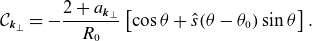 \begin{equation} \mathcal{C}_{{\boldsymbol{k}}_\perp } = -\frac {2+a_{{\boldsymbol{k}}_\perp }}{R_0} \left [\cos \theta + \hat {s}(\theta -\theta _0)\sin \theta \right ]. \end{equation}
In the above, $\psi _0$
and
$\psi _0$
and $\alpha _0$
are the coordinates of the field line at
$\alpha _0$
are the coordinates of the field line at $x=y=0$
,
$x=y=0$
, $q_0 = q(\psi _0)$
is the safety factor,
$q_0 = q(\psi _0)$
is the safety factor, $R_0$
and
$R_0$
and $r_0$
are the major and minor radius of its flux surface, respectively,
$r_0$
are the major and minor radius of its flux surface, respectively, $B_0$
is any suitable normalising magnetic field,
$B_0$
is any suitable normalising magnetic field, $\hat {s} = (r_0/q_0)\textrm {d} q / \textrm {d} r$
is the magnetic shear at
$\hat {s} = (r_0/q_0)\textrm {d} q / \textrm {d} r$
is the magnetic shear at $r=r_0$
, and
$r=r_0$
, and $\theta _0 = -k_x/\hat {s}k_y$
is the poloidal angle at which the radial projection of the wavenumber vanishes, viz.
$\theta _0 = -k_x/\hat {s}k_y$
is the poloidal angle at which the radial projection of the wavenumber vanishes, viz. ${{\boldsymbol{k}}_\perp }(\theta _0)\boldsymbol{\cdot }{\boldsymbol{\nabla }} x = 0$
.
${{\boldsymbol{k}}_\perp }(\theta _0)\boldsymbol{\cdot }{\boldsymbol{\nabla }} x = 0$
.
In figure 1, we plot (2.36) for different values of $\hat {s}$
and
$\hat {s}$
and $\theta _0$
. Figure 1(a) shows the simplest case of zero magnetic shear (
$\theta _0$
. Figure 1(a) shows the simplest case of zero magnetic shear ( $\hat {s} = 0$
), wherein the local magnetic curvature
$\hat {s} = 0$
), wherein the local magnetic curvature
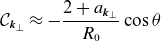 \begin{equation} \mathcal{C}_{{\boldsymbol{k}}_\perp } \approx -\frac {2+a_{{\boldsymbol{k}}_\perp }}{R_0} \cos \theta \end{equation}
is independent of $\theta _0$
. In this case, the regions of good and bad curvature coincide perfectly with the inboard and outboard sides of the device, respectively. Figures 1(b) and 1(c) demonstrate the inherent symmetry of (2.36) whereby the local effective magnetic curvature
$\theta _0$
. In this case, the regions of good and bad curvature coincide perfectly with the inboard and outboard sides of the device, respectively. Figures 1(b) and 1(c) demonstrate the inherent symmetry of (2.36) whereby the local effective magnetic curvature $\mathcal{C}_{{\boldsymbol{k}}_\perp }$
changes from bad to good (or vice versa) as a function of
$\mathcal{C}_{{\boldsymbol{k}}_\perp }$
changes from bad to good (or vice versa) as a function of $\theta - \theta _0$
if the mode is ‘reflected’ to the diametrically opposite side of the flux surface. More concretely,
$\theta - \theta _0$
if the mode is ‘reflected’ to the diametrically opposite side of the flux surface. More concretely, $\mathcal{C}_{{\boldsymbol{k}}_\perp } \mapsto -\mathcal{C}_{{\boldsymbol{k}}_\perp }$
under the mapping
$\mathcal{C}_{{\boldsymbol{k}}_\perp } \mapsto -\mathcal{C}_{{\boldsymbol{k}}_\perp }$
under the mapping $\theta \mapsto \theta + \pi$
and
$\theta \mapsto \theta + \pi$
and $\theta _0 \mapsto \theta _0 + \pi$
, which is evident from (2.36).
$\theta _0 \mapsto \theta _0 + \pi$
, which is evident from (2.36).
Note that the definition of good and bad curvature as $\mathcal{C}_{{\boldsymbol{k}}_\perp } \gt 0$
or
$\mathcal{C}_{{\boldsymbol{k}}_\perp } \gt 0$
or $\mathcal{C}_{{\boldsymbol{k}}_\perp } \lt 0$
is mode-specific because (2.37) [and, indeed, (2.30)] depends explicitly on the structure of the mode via
$\mathcal{C}_{{\boldsymbol{k}}_\perp } \lt 0$
is mode-specific because (2.37) [and, indeed, (2.30)] depends explicitly on the structure of the mode via $a_{{\boldsymbol{k}}_\perp }$
. Indeed,
$a_{{\boldsymbol{k}}_\perp }$
. Indeed, $a_{{\boldsymbol{k}}_\perp } \lt -2$
reverses the relationship between the sign of
$a_{{\boldsymbol{k}}_\perp } \lt -2$
reverses the relationship between the sign of $\mathcal{C}_{{\boldsymbol{k}}_\perp }$
and the outboard/inboard location in the toroidal geometry. However, this is a rather exotic scenario wherein the parallel and perpendicular heat fluxes have opposite signs [see also (2.34) and the discussion surrounding it]. As far as the authors are aware, no such instabilities are known to exist in fusion plasmas.
$\mathcal{C}_{{\boldsymbol{k}}_\perp }$
and the outboard/inboard location in the toroidal geometry. However, this is a rather exotic scenario wherein the parallel and perpendicular heat fluxes have opposite signs [see also (2.34) and the discussion surrounding it]. As far as the authors are aware, no such instabilities are known to exist in fusion plasmas.
Panels (a) to (c) visualise the circular-flux-surface local curvature (2.36) as a function of $\theta$
for three different values of
$\theta$
for three different values of $\hat {s}$
and
$\hat {s}$
and $\theta _0$
, as indicated in the title of each panel. The regions of good and bad local curvature are shaded in blue and red, respectively. The grey shaded regions correspond to the outboard side of the device, viz.
$\theta _0$
, as indicated in the title of each panel. The regions of good and bad local curvature are shaded in blue and red, respectively. The grey shaded regions correspond to the outboard side of the device, viz. $-\pi /2 + 2\pi n \lt \theta \lt \pi /2 + 2\pi n$
for some
$-\pi /2 + 2\pi n \lt \theta \lt \pi /2 + 2\pi n$
for some $n \in \mathbb{Z}$
.
$n \in \mathbb{Z}$
.
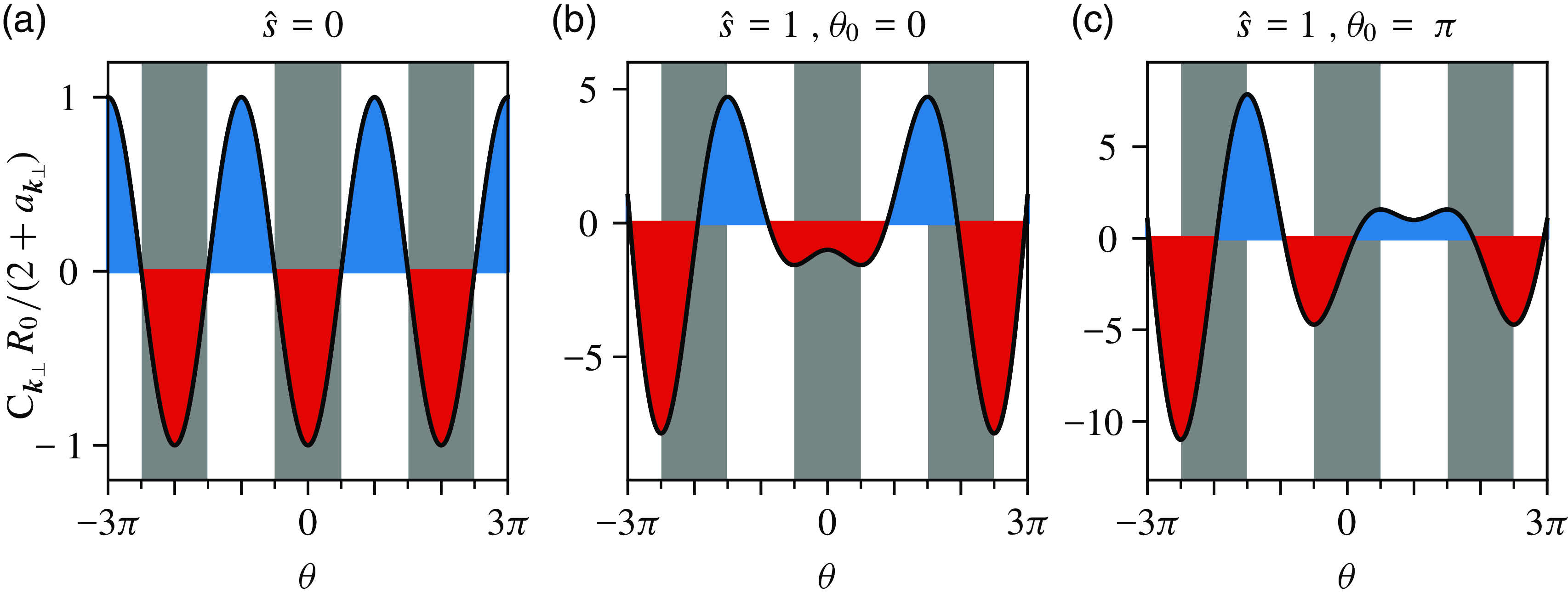
2.4.2. The
$Z$
-pinch

An even simpler description of curvature-driven modes can be obtained by ignoring entirely the variation of the field along $z$
. Sometimes called the ‘local kinetic approximation’ (Terry et al. Reference Terry, Anderson and Horton1982; Romanelli Reference Romanelli1989; Zocco et al. Reference Zocco, Xanthopoulos, Doerk, Connor and Helander2018), this is equivalent to the magnetic geometry of a
$z$
. Sometimes called the ‘local kinetic approximation’ (Terry et al. Reference Terry, Anderson and Horton1982; Romanelli Reference Romanelli1989; Zocco et al. Reference Zocco, Xanthopoulos, Doerk, Connor and Helander2018), this is equivalent to the magnetic geometry of a $Z$
-pinch if we also ignore the radial magnetic drifts. This
$Z$
-pinch if we also ignore the radial magnetic drifts. This $Z$
-pinch geometry is the minimal model for curvature-driven instabilities in the absence of trapped-particle effects and has been a popular setting for simple models of both linear and nonlinear physics (Ricci, Rogers & Dorland Reference Ricci, Rogers and Dorland2006; Kobayashi & Rogers Reference Kobayashi and Rogers2012; Kobayashi, Gürcan & Diamond Reference Kobayashi, Gürcan and Diamond2015; Ivanov et al. Reference Ivanov, Schekochihin, Dorland, Field and Parra2020, Reference Ivanov, Schekochihin and Dorland2022; Adkins et al. Reference Adkins, Schekochihin, Ivanov and Roach2022; Hallenbert & Plunk Reference Hallenbert and Plunk2022; Adkins, Ivanov & Schekochihin Reference Adkins, Ivanov and Schekochihin2023; Ivanov & Adkins Reference Ivanov and Adkins2023; Hoffmann, Frei & Ricci Reference Hoffmann, Frei and Ricci2023).
$Z$
-pinch geometry is the minimal model for curvature-driven instabilities in the absence of trapped-particle effects and has been a popular setting for simple models of both linear and nonlinear physics (Ricci, Rogers & Dorland Reference Ricci, Rogers and Dorland2006; Kobayashi & Rogers Reference Kobayashi and Rogers2012; Kobayashi, Gürcan & Diamond Reference Kobayashi, Gürcan and Diamond2015; Ivanov et al. Reference Ivanov, Schekochihin, Dorland, Field and Parra2020, Reference Ivanov, Schekochihin and Dorland2022; Adkins et al. Reference Adkins, Schekochihin, Ivanov and Roach2022; Hallenbert & Plunk Reference Hallenbert and Plunk2022; Adkins, Ivanov & Schekochihin Reference Adkins, Ivanov and Schekochihin2023; Ivanov & Adkins Reference Ivanov and Adkins2023; Hoffmann, Frei & Ricci Reference Hoffmann, Frei and Ricci2023).
In this geometry, we take $(x, y, z)$
to be local Cartesian coordinates, where
$(x, y, z)$
to be local Cartesian coordinates, where $z$
is now the distance along the field lines, and define the gradient scale length of the magnetic field
$z$
is now the distance along the field lines, and define the gradient scale length of the magnetic field $B = B(x)$
:
$B = B(x)$
:
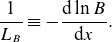 \begin{equation} \frac {1}{{L_B}} \equiv -\frac {\textrm {d}\,{\ln B}}{\textrm {d}{x}}. \end{equation}
Hence, we obtain
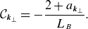 \begin{equation} \mathcal{C}_{{\boldsymbol{k}}_\perp } = -\frac {2+a_{{\boldsymbol{k}}_\perp }}{{L_B}}. \end{equation}
Therefore, in the $Z$
-pinch geometry,
$Z$
-pinch geometry, ${L_B} \lt 0$
and
${L_B} \lt 0$
and ${L_B} \gt 0$
correspond to good and bad curvature, respectively. As discussed before, we expect to find electrostatic curvature-driven instabilities only in the case
${L_B} \gt 0$
correspond to good and bad curvature, respectively. As discussed before, we expect to find electrostatic curvature-driven instabilities only in the case ${L_B} \gt 0$
(note that we are still assuming
${L_B} \gt 0$
(note that we are still assuming $L_{T_{s}} \gt 0$
). In the next section, we present an example of an electromagnetic instability in the
$L_{T_{s}} \gt 0$
). In the next section, we present an example of an electromagnetic instability in the $Z$
-pinch geometry that exists exclusively in good-curvature regions, viz.
$Z$
-pinch geometry that exists exclusively in good-curvature regions, viz. ${L_B} \lt 0$
.
${L_B} \lt 0$
.
3. Low-
$\beta$
, drift-kinetic fluctuations in the local kinetic limit

3.1. Ordering and equations
Our goal is to simplify the GK equation (2.4) in order to distil a minimum model for the good-curvature electromagnetic instability discussed in § 3.2.2. We limit ourselves to the low- $\beta$
, zero-magnetic-shear,
$\beta$
, zero-magnetic-shear, $Z$
-pinch geometry, and consider fluctuations that obey the ordering
$Z$
-pinch geometry, and consider fluctuations that obey the ordering
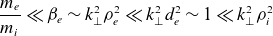 \begin{equation} \frac {m_{e}}{m_{i}}\ll \beta _{e} \sim k_\perp ^2\rho _{e}^2 \ll k_\perp ^2d_{e}^2 \sim 1 \ll k_\perp ^2 \rho _{i}^2 \end{equation}
and evolve on time scales
 \begin{equation} \omega \sim k_\parallel v_{\text{th}{e}} \sim \omega _{*{e}} \sim \omega _{T{e}} \sim \omega _{\text{d}e} \end{equation}
in a plasma of two species, electrons and ions. The drift frequencies in (3.2) are
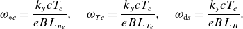 \begin{align} \omega _{*{e}} = \frac {k_y c T_{e}}{e B L_{n_{e}}}, \quad \omega _{T{e}} = \frac {k_y c T_{e}}{e B L_{T_{e}}}, \quad \omega _{\text{d}s} = \frac {k_y c T_{e}}{e B {L_B}}. \end{align}
In Appendix C, we show that, under the above assumptions, the fluctuations obey the electron drift-kinetic equation [see (C.12)]. Under the low- $\beta$
assumption,
$\beta$
assumption, $\delta B_\parallel$
is small and this drift-kinetic equation is closed by quasineutrality (2.7) and the parallel component of Ampère’s law (2.8) [see (C.13) and (C.14), respectively]. In Appendix C.1, we derive the forms of the free-energy and field-invariant conservation laws under the orderings (3.1) and (3.2). As expected, the free energy is a positive-definite quantity, injected by the radial heat flux. In contrast, the field invariant contains negative-definite electrostatic and positive-definite electromagnetic contributions. It is injected by the slab term, proportional to
$\delta B_\parallel$
is small and this drift-kinetic equation is closed by quasineutrality (2.7) and the parallel component of Ampère’s law (2.8) [see (C.13) and (C.14), respectively]. In Appendix C.1, we derive the forms of the free-energy and field-invariant conservation laws under the orderings (3.1) and (3.2). As expected, the free energy is a positive-definite quantity, injected by the radial heat flux. In contrast, the field invariant contains negative-definite electrostatic and positive-definite electromagnetic contributions. It is injected by the slab term, proportional to $k_\parallel$
, and by the curvature term, proportional to the magnetic-field gradient (2.38) and the radial heat flux.
$k_\parallel$
, and by the curvature term, proportional to the magnetic-field gradient (2.38) and the radial heat flux.
In Appendix D, we outline the derivation of the dispersion relation for the low- $\beta$
, drift-kinetic fluctuations. In the three-dimensional case (viz.
$\beta$
, drift-kinetic fluctuations. In the three-dimensional case (viz. $k_\parallel \neq 0$
), the dispersion relation is given by unwieldy and mostly unenlightening expressions that can be found in Appendix D. We now focus on the two-dimensional case, which represents a minimal model for (at least one example of) the good-curvature-driven instabilities.
$k_\parallel \neq 0$
), the dispersion relation is given by unwieldy and mostly unenlightening expressions that can be found in Appendix D. We now focus on the two-dimensional case, which represents a minimal model for (at least one example of) the good-curvature-driven instabilities.
3.2. Two-dimensional fluctuations
In the two-dimensional limit, viz. $k_\parallel = 0$
, the electron drift-kinetic equation decouples into its even and an odd parts in
$k_\parallel = 0$
, the electron drift-kinetic equation decouples into its even and an odd parts in $v_\parallel$
[see (C.15) and (C.16)]. The former, together with quasineutrality, describes purely electrostatic (
$v_\parallel$
[see (C.15) and (C.16)]. The former, together with quasineutrality, describes purely electrostatic ( $\delta A_\parallel = 0$
) modes. Their dispersion relation is found to be
$\delta A_\parallel = 0$
) modes. Their dispersion relation is found to be
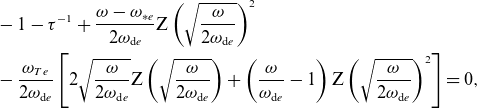 \begin{align} &-1-\tau ^{-1}+\frac {\omega -\omega _{*{e}}}{2\omega _{\text{d}e}}\textrm {Z}\left (\sqrt {\frac {\omega }{2\omega _{\text{d}e}}}\right )^2 \nonumber \\ &- \frac {\omega _{T{e}}}{2\omega _{\text{d}e}}\left [2\sqrt {\frac {\omega }{2\omega _{\text{d}e}}}\textrm {Z}\left (\sqrt {\frac {\omega }{2\omega _{\text{d}e}}}\right ) + \left (\frac {\omega }{\omega _{\text{d}e}}-1\right )\textrm {Z}\left (\sqrt {\frac {\omega }{2\omega _{\text{d}e}}}\right )^2\right ] = 0, \end{align}
where $\tau \equiv eT_{i} / q_{i} T_{e}$
and
$\tau \equiv eT_{i} / q_{i} T_{e}$
and $\textrm {Z}(\zeta )$
is the usual plasma dispersion function (Faddeeva & Terent’ev Reference Faddeeva and Terent’ev1954; Fried & Conte Reference Fried and Conte1961) given by
$\textrm {Z}(\zeta )$
is the usual plasma dispersion function (Faddeeva & Terent’ev Reference Faddeeva and Terent’ev1954; Fried & Conte Reference Fried and Conte1961) given by
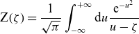 \begin{equation} \textrm {Z}(\zeta ) = \frac {1}{\sqrt {\pi }} \int _{-\infty }^{+\infty } \textrm {d} {u} \frac {\textrm {e}^{-u^2}}{u - \zeta } \end{equation}
for $\text{Im}(\zeta ) \gt 0$
and analytically continued to the entire complex plane. Equation (3.4) is the same as the dispersion relation derived by Biglari et al. (Reference Biglari, Diamond and Rosenbluth1989) and Zocco et al. (Reference Zocco, Xanthopoulos, Doerk, Connor and Helander2018) for the electrostatic cITG instability, up to replacing
$\text{Im}(\zeta ) \gt 0$
and analytically continued to the entire complex plane. Equation (3.4) is the same as the dispersion relation derived by Biglari et al. (Reference Biglari, Diamond and Rosenbluth1989) and Zocco et al. (Reference Zocco, Xanthopoulos, Doerk, Connor and Helander2018) for the electrostatic cITG instability, up to replacing $\tau \mapsto \tau ^{-1}$
and
$\tau \mapsto \tau ^{-1}$
and $i \mapsto e$
, which accounts for the fact that we are dealing with cETG instead. The solutions to (3.4) contain the familiar cETG modes that require bad magnetic curvature to be unstable.
$i \mapsto e$
, which accounts for the fact that we are dealing with cETG instead. The solutions to (3.4) contain the familiar cETG modes that require bad magnetic curvature to be unstable.
The odd part of the electron drift-kinetic equation and parallel Ampère’s law also form a closed system, this time of purely electromagnetic ( $\phi = 0$
) modes. Physically, these are fluctuations with no density or temperature perturbations but a nonzero parallel current. Their dispersion relation is
$\phi = 0$
) modes. Physically, these are fluctuations with no density or temperature perturbations but a nonzero parallel current. Their dispersion relation is
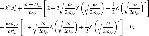 \begin{align} &-k_\perp ^2d_{e}^2 + \frac {\omega - \omega _{*{e}}}{\omega _{\text{d}e}} \left [2 + 2\sqrt {\frac {\omega }{2\omega _{\text{d}e}}}\textrm {Z}\left (\sqrt {\frac {\omega }{2\omega _{\text{d}e}}}\right ) + \frac {1}{2}\textrm {Z}\left (\sqrt {\frac {\omega }{2\omega _{\text{d}e}}}\right )^2 \right ] \nonumber \\ &-\frac {\omega \omega _{T{e}}}{\omega _{\text{d}e}^2}\left [1 + \sqrt {\frac {\omega }{2\omega _{\text{d}e}}}\textrm {Z}\left (\sqrt {\frac {\omega }{2\omega _{\text{d}e}}}\right ) +\frac {1}{2}\textrm {Z}\left (\sqrt {\frac {\omega }{2\omega _{\text{d}e}}}\right )^2 \right ]=0. \end{align}
The appearance of a square root in (3.4) and (3.6) means that additional care must be taken due to the presence of a branch cut in the complex plane. This is a well-known problem (Kim et al. Reference Kim, Kishimoto, Horton and Tajima1994; Kuroda et al. Reference Kuroda, Sugama, Kanno, Okamoto and Horton1998; Sugama Reference Sugama1999; Helander et al. Reference Helander, Mishchenko, Kleiber and Xanthopoulos2011; Mishchenko, Plunk & Helander Reference Mishchenko, Plunk and Helander2018) stemming from the presence of the magnetic drifts. The square-root branch must be chosen so that it agrees with the principal branch of the square-root function in the upper-half of the complex plane. Its branch cut can be anywhere in the lower-half of the complex $\omega$
plane. More details on how to handle the branch cuts and the analytic continuation of the dispersion relation in a
$\omega$
plane. More details on how to handle the branch cuts and the analytic continuation of the dispersion relation in a $Z$
-pinch can be found in Ivanov & Adkins (Reference Ivanov and Adkins2023).
$Z$
-pinch can be found in Ivanov & Adkins (Reference Ivanov and Adkins2023).
To avoid the complications arising from the square root, we have chosen to fix the sign of the magnetic-field gradient to $\omega _{\text{d}e} \gt 0$
. This is necessary in order to put
$\omega _{\text{d}e} \gt 0$
. This is necessary in order to put $\omega _{\text{d}e}$
under the square root in (3.4) and (3.6). With this choice, ‘bad curvature’ corresponds to
$\omega _{\text{d}e}$
under the square root in (3.4) and (3.6). With this choice, ‘bad curvature’ corresponds to $\omega _{T{e}} \gt 0$
, ‘good curvature’ to
$\omega _{T{e}} \gt 0$
, ‘good curvature’ to $\omega _{T{e}} \lt 0$
. This differs from our discussion in §§ 2.4 and 2.4.2 where we fixed the sign of the temperature-gradient length scale
$\omega _{T{e}} \lt 0$
. This differs from our discussion in §§ 2.4 and 2.4.2 where we fixed the sign of the temperature-gradient length scale $L_{T_{s}}$
but varied the local sign of the magnetic gradient. Note that we will only investigate equilibria in which the temperature and density gradients are aligned, i.e.
$L_{T_{s}}$
but varied the local sign of the magnetic gradient. Note that we will only investigate equilibria in which the temperature and density gradients are aligned, i.e. $L_{T_{s}}$
and
$L_{T_{s}}$
and $L_{n_{s}}$
will always have the same relative sign.
$L_{n_{s}}$
will always have the same relative sign.
Before we investigate the novel, good-curvature electromagnetic instability that is about to emerge, let us recap some of the properties of the more widely known electrostatic cETG instability. This will be useful later on in order to compare and contrast the electrostatic and electromagnetic curvature-driven instabilities.
3.2.1. Two-dimensional cETG instability
In the two-dimensional limit, the electrostatic dispersion relation (3.4) has three independent parameters, which are the temperature ratio $\tau$
and the normalised equilibrium gradients
$\tau$
and the normalised equilibrium gradients
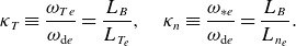 \begin{equation} \kappa _T \equiv \frac {\omega _{T{e}}}{\omega _{\text{d}e}} = \frac {{L_B}}{L_{T_{e}}}, \quad \kappa _n \equiv \frac {\omega _{*{e}}}{\omega _{\text{d}e}} = \frac {{L_B}}{L_{n_{e}}}. \end{equation}
In this notation, $\kappa _T \gt 0$
corresponds to bad magnetic curvature. Note that if we normalise
$\kappa _T \gt 0$
corresponds to bad magnetic curvature. Note that if we normalise $\omega$
to any of the diamagnetic frequencies (or, indeed, a combination of them), then the dispersion relation for the normalised frequency is independent of the perpendicular wavenumber
$\omega$
to any of the diamagnetic frequencies (or, indeed, a combination of them), then the dispersion relation for the normalised frequency is independent of the perpendicular wavenumber ${\boldsymbol{k}}_\perp$
. Equivalently, any linear solution to the (electrostatic) electron drift-kinetic equation (C.15) obeys
${\boldsymbol{k}}_\perp$
. Equivalently, any linear solution to the (electrostatic) electron drift-kinetic equation (C.15) obeys $\omega \propto k_y$
. This is a reflection of the scale invariance of electrostatic drift kinetics (Adkins et al. Reference Adkins, Ivanov and Schekochihin2023), which is only broken at small scales by the finite-Larmor-radius effects (viz. the Bessel functions) that we neglected in § 3.1. Figure 2 shows the growth rate and frequency of the unstable cETG mode. The instability exists only when
$\omega \propto k_y$
. This is a reflection of the scale invariance of electrostatic drift kinetics (Adkins et al. Reference Adkins, Ivanov and Schekochihin2023), which is only broken at small scales by the finite-Larmor-radius effects (viz. the Bessel functions) that we neglected in § 3.1. Figure 2 shows the growth rate and frequency of the unstable cETG mode. The instability exists only when $\kappa _T \gt \kappa _{T\text{crit}}$
, where
$\kappa _T \gt \kappa _{T\text{crit}}$
, where $\kappa _{T\text{crit}} \gt 0$
is some positive critical temperature gradient that depends on
$\kappa _{T\text{crit}} \gt 0$
is some positive critical temperature gradient that depends on $\tau$
and
$\tau$
and $\kappa _n$
. Additionally, the (real) frequency of the cETG mode satisfies
$\kappa _n$
. Additionally, the (real) frequency of the cETG mode satisfies $\text{Re}(\omega )/\omega _{T{e}} \gt 0$
, i.e. the phase velocity of the mode is in the electron diamagnetic direction.
$\text{Re}(\omega )/\omega _{T{e}} \gt 0$
, i.e. the phase velocity of the mode is in the electron diamagnetic direction.
Growth rate (a) and frequency (b) of the cETG mode as a function of the normalised temperature gradient $\kappa _T$
and inverse temperature ratio
$\kappa _T$
and inverse temperature ratio $\tau ^{-1}$
at zero density gradient (
$\tau ^{-1}$
at zero density gradient ( $\kappa _n = 0$
). These are the solutions of (3.4). The growth rate and frequency have been normalised by the fluid growth rate (3.9). Only the unstable, i.e.
$\kappa _n = 0$
). These are the solutions of (3.4). The growth rate and frequency have been normalised by the fluid growth rate (3.9). Only the unstable, i.e. $\text{Im}\:\omega \gt 0$
, region is shown.
$\text{Im}\:\omega \gt 0$
, region is shown.
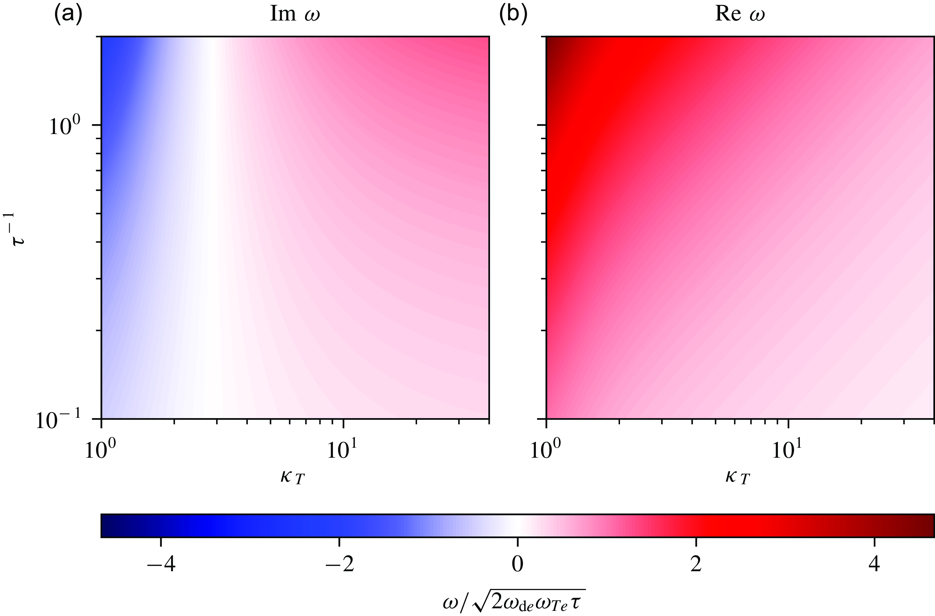
A key characteristic of the cETG instability is that it has a physically transparent ‘fluid’ limit. Mathematically, this limit corresponds to $\omega \gg \omega _{\text{d}e}$
, wherein we can use the asymptotic expansion
$\omega \gg \omega _{\text{d}e}$
, wherein we can use the asymptotic expansion
 \begin{equation} \textrm {Z}(\zeta ) \sim -\frac {1}{\zeta } -\frac {1}{2\zeta ^3} - \frac {3}{4\zeta ^5} + O\left ({\zeta ^{-7}}\right ), \end{equation}
valid for $\left \rvert {\zeta }\right \rvert \gg 1$
and
$\left \rvert {\zeta }\right \rvert \gg 1$
and $\text{Im}\:\zeta \gt 0$
. The electrostatic dispersion relation (3.4) then simplifies to
$\text{Im}\:\zeta \gt 0$
. The electrostatic dispersion relation (3.4) then simplifies to
 \begin{equation} \omega ^2 = -2\omega _{T{e}}\omega _{\text{d}e}\tau . \end{equation}
This is the well-known fluid cETG dispersion relation (Pogutse Reference Pogutse1968; Horton, Hong & Tang Reference Horton, Hong and Tang1988) that yields unstable solutions only if the curvature is bad, i.e. if $\omega _{T{e}}$
and
$\omega _{T{e}}$
and $\omega _{\text{d}e}$
have the same sign (or, equivalently,
$\omega _{\text{d}e}$
have the same sign (or, equivalently, $\kappa _T \gt 0$
). Evidently, the ‘fluid’ assumption
$\kappa _T \gt 0$
). Evidently, the ‘fluid’ assumption $\omega \gg \omega _{\text{d}e}$
is consistent with (3.9) only in the strongly driven regime
$\omega \gg \omega _{\text{d}e}$
is consistent with (3.9) only in the strongly driven regime $\omega _{T{e}} \gg \omega _{\text{d}e}$
.
$\omega _{T{e}} \gg \omega _{\text{d}e}$
.
The ‘fluidisation’ of ETG in the limit $\omega \gg \omega _{\text{d}e}$
can be justified rigorously by performing a systematic decomposition of the drift-kinetic equation into an infinite hierarchy of fluid moments. One popular way of doing this is the Hermite–Laguerre decomposition (Smith Reference Smith1997; Watanabe & Sugama Reference Watanabe and Sugama2004; Zocco & Schekochihin Reference Zocco and Schekochihin2011; Zocco et al. Reference Zocco, Loureiro, Dickinson, Numata and Roach2015; Loureiro et al. Reference Loureiro, Dorland, Fazendeiro, Kanekar, Mallet, Vilelas and Zocco2016; Mandell, Dorland & Landreman Reference Mandell, Dorland and Landreman2018; Adkins et al. Reference Adkins, Schekochihin, Ivanov and Roach2022; Frei et al. Reference Frei, Ernst and Ricci2022, Reference Frei, Hoffmann, Ricci, Brunner and Tecchioll2023; Mischenko Reference Mischenko2024). In the limit where the mode frequency is much larger than the ‘kinetic’ frequencies
$\omega \gg \omega _{\text{d}e}$
can be justified rigorously by performing a systematic decomposition of the drift-kinetic equation into an infinite hierarchy of fluid moments. One popular way of doing this is the Hermite–Laguerre decomposition (Smith Reference Smith1997; Watanabe & Sugama Reference Watanabe and Sugama2004; Zocco & Schekochihin Reference Zocco and Schekochihin2011; Zocco et al. Reference Zocco, Loureiro, Dickinson, Numata and Roach2015; Loureiro et al. Reference Loureiro, Dorland, Fazendeiro, Kanekar, Mallet, Vilelas and Zocco2016; Mandell, Dorland & Landreman Reference Mandell, Dorland and Landreman2018; Adkins et al. Reference Adkins, Schekochihin, Ivanov and Roach2022; Frei et al. Reference Frei, Ernst and Ricci2022, Reference Frei, Hoffmann, Ricci, Brunner and Tecchioll2023; Mischenko Reference Mischenko2024). In the limit where the mode frequency is much larger than the ‘kinetic’ frequencies $k_\parallel v_{\text{th}{e}}$
and
$k_\parallel v_{\text{th}{e}}$
and $\omega _{\text{d}e}$
, the moment hierarchy is naturally truncated to the six lowest-order fluid moments listed in Appendix A.5.4 of Adkins et al. (Reference Adkins, Schekochihin, Ivanov and Roach2022). Reducing this to the two-dimensional limit (
$\omega _{\text{d}e}$
, the moment hierarchy is naturally truncated to the six lowest-order fluid moments listed in Appendix A.5.4 of Adkins et al. (Reference Adkins, Schekochihin, Ivanov and Roach2022). Reducing this to the two-dimensional limit ( $k_\parallel = 0$
), we find a closed system of fluid equations describing the perturbations of the electron density
$k_\parallel = 0$
), we find a closed system of fluid equations describing the perturbations of the electron density $\delta n_{e}$
, parallel temperature
$\delta n_{e}$
, parallel temperature $\delta T_{\parallel {e}}$
and perpendicular temperature
$\delta T_{\parallel {e}}$
and perpendicular temperature $\delta T_{\perp {e}}$
(Adkins et al. Reference Adkins, Schekochihin, Ivanov and Roach2022), as follows:
$\delta T_{\perp {e}}$
(Adkins et al. Reference Adkins, Schekochihin, Ivanov and Roach2022), as follows:
 \begin{align} &\frac {\partial }{\partial t}\frac {\delta n_{e{\boldsymbol{k}}}}{{n_{e}}} + \textrm {i} \omega _{\text{d}e}\left (\frac {\delta T_{\parallel {e}{\boldsymbol{k}}}}{T_{e}} + \frac {\delta T_{\perp {e}{\boldsymbol{k}}}}{T_{e}}\right ) = 0, \end{align}
 \begin{align} &\frac {\partial }{\partial t}\frac {\delta T_{\parallel {e}{\boldsymbol{k}}}}{T_{e}} + \textrm {i} \omega _{T{e}} \frac {e{\phi }_{\boldsymbol{k}}}{T_{e}} = 0, \end{align}
 \begin{align} &\frac {\partial }{\partial t}\frac {\delta T_{\perp {e}{\boldsymbol{k}}}}{T_{e}} + \textrm {i} \omega _{T{e}} \frac {e{\phi }_{\boldsymbol{k}}}{T_{e}} = 0, \\[6pt] \nonumber \end{align}
where the density and electrostatic potential are related by $\delta n_{e{\boldsymbol{k}}}/{n_{e}} = -e{\phi }_{\boldsymbol{k}} / \tau T_{e}$
. The system (3.10)–(3.12) is the minimal fluid model for the strongly driven, two-dimensional, electrostatic collisionless cETG instability. It is straightforward to confirm that its dispersion relation is (3.9). The fluidisation of cETG is discussed further in Appendix E.
$\delta n_{e{\boldsymbol{k}}}/{n_{e}} = -e{\phi }_{\boldsymbol{k}} / \tau T_{e}$
. The system (3.10)–(3.12) is the minimal fluid model for the strongly driven, two-dimensional, electrostatic collisionless cETG instability. It is straightforward to confirm that its dispersion relation is (3.9). The fluidisation of cETG is discussed further in Appendix E.
3.2.2. Two-dimensional MDM
The electromagnetic dispersion relation (3.6) has three independent parameters, which are $k_\perp ^2d_{e}^2$
and the normalised gradients (3.7). Note that, in contrast with the electrostatic case, the perpendicular wavenumber enters explicitly as a parameter because the presence of the electron skin depth
$k_\perp ^2d_{e}^2$
and the normalised gradients (3.7). Note that, in contrast with the electrostatic case, the perpendicular wavenumber enters explicitly as a parameter because the presence of the electron skin depth $d_{e}$
breaks the scale invariance of the equations. Figure 3 shows the growth rate and frequency of the unstable solutions of (3.6) as a function of
$d_{e}$
breaks the scale invariance of the equations. Figure 3 shows the growth rate and frequency of the unstable solutions of (3.6) as a function of $k_\perp ^2d_{e}^2$
and
$k_\perp ^2d_{e}^2$
and $\kappa _T$
. The instability is present only when
$\kappa _T$
. The instability is present only when $\kappa _T \lt 0$
, i.e. when the magnetic curvature is good. This is the MDM. There are three stability boundaries, where the growth rate of the MDM vanishes. The details of their derivation can be found in Appendix F.
$\kappa _T \lt 0$
, i.e. when the magnetic curvature is good. This is the MDM. There are three stability boundaries, where the growth rate of the MDM vanishes. The details of their derivation can be found in Appendix F.
Growth rate (a) and frequency (b) of the MDM as a function of $k_\perp ^2d_{e}^2$
and
$k_\perp ^2d_{e}^2$
and $\kappa _T$
at
$\kappa _T$
at $\kappa _n = -1$
. These are the solutions of (3.6). The solid black lines are the stability boundaries, on which
$\kappa _n = -1$
. These are the solutions of (3.6). The solid black lines are the stability boundaries, on which $\text{Im}\:\omega =0$
. Their asymptotic slopes at large
$\text{Im}\:\omega =0$
. Their asymptotic slopes at large $\kappa _T$
are given by (3.15) and (3.16). On the horizontal dotted grey line, the MDM root of (3.6) is
$\kappa _T$
are given by (3.15) and (3.16). On the horizontal dotted grey line, the MDM root of (3.6) is $\omega = 0$
. The value of
$\omega = 0$
. The value of $k_\perp ^2d_{e}^2$
there is given by (3.13). The vertical dashed–dotted grey lines denote the ends of the solid black stability boundaries and are given by the limits of the black dashed line (3.14). In the hatched region, there does not exist a unique root that is continuously connected to the unstable MDM solution, thus we have omitted that part of the plot [see also the discussion after (3.16)].
$k_\perp ^2d_{e}^2$
there is given by (3.13). The vertical dashed–dotted grey lines denote the ends of the solid black stability boundaries and are given by the limits of the black dashed line (3.14). In the hatched region, there does not exist a unique root that is continuously connected to the unstable MDM solution, thus we have omitted that part of the plot [see also the discussion after (3.16)].
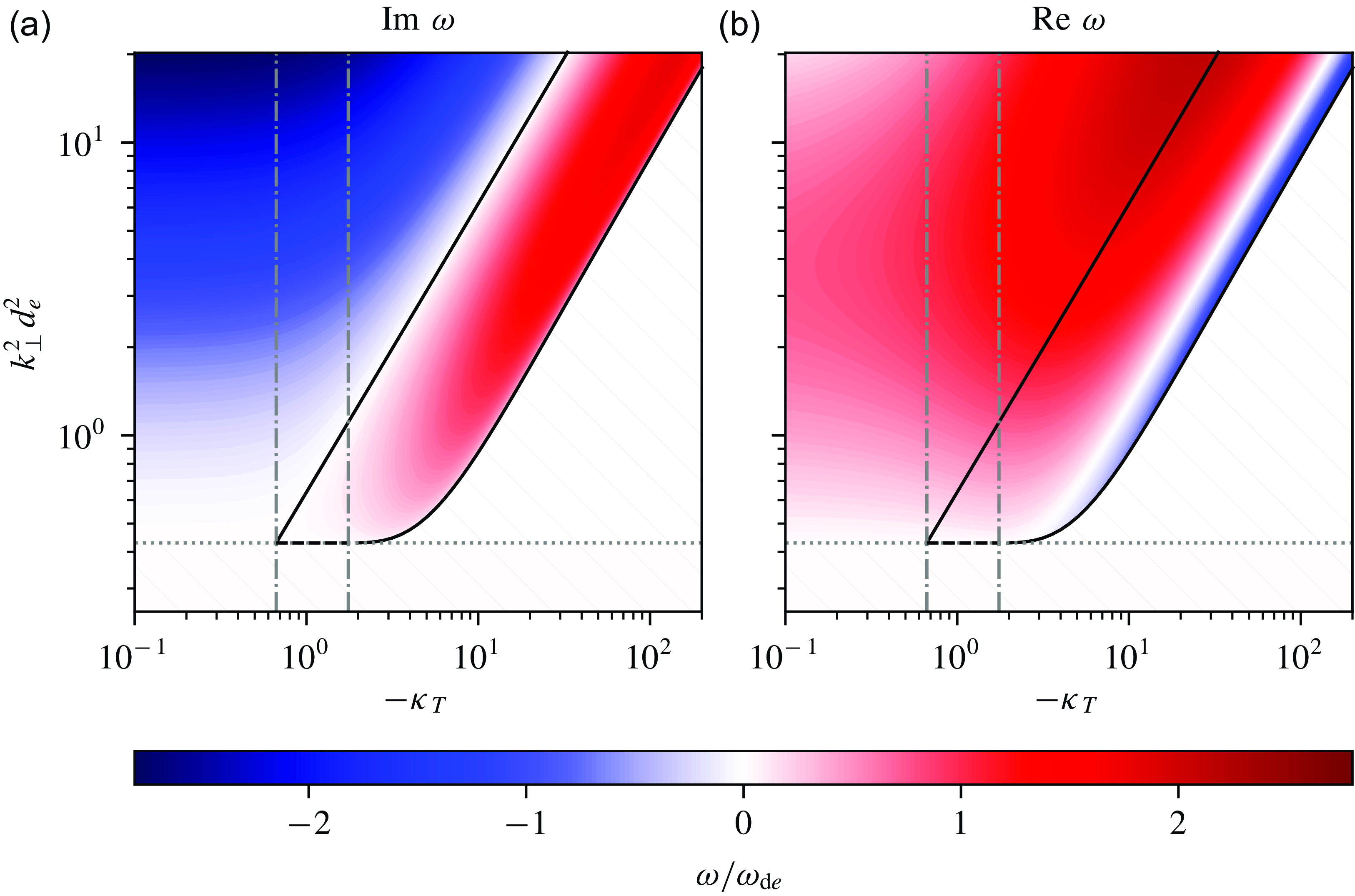
The first of these (the dotted grey line in figure 3) lies at $k_\perp ^2d_{e}^2 = k_{\perp \text{,min}}^2d_{e}^2$
, where
$k_\perp ^2d_{e}^2 = k_{\perp \text{,min}}^2d_{e}^2$
, where
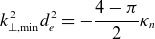 \begin{equation} k_{\perp \text{,min}}^2d_{e}^2 = -\frac {4-\pi }{2}\kappa _n \end{equation}
and is bounded by
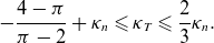 \begin{equation} -\frac {4-\pi }{\pi -2} + \kappa _n \leqslant \kappa _T \leqslant \frac {2}{3}\kappa _n. \end{equation}
On this line, $\omega = 0$
, i.e. both the frequency and growth rate of the MDM vanish. Note that, as promised above, we only consider equilibria where the temperature and density gradients are aligned. In particular, if
$\omega = 0$
, i.e. both the frequency and growth rate of the MDM vanish. Note that, as promised above, we only consider equilibria where the temperature and density gradients are aligned. In particular, if $\kappa _T$
is negative, then so is
$\kappa _T$
is negative, then so is $\kappa _n$
.
$\kappa _n$
.
The upper stability boundary (the solid black line in figure 3) asymptotes to
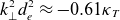 \begin{equation} k_\perp ^2d_{e}^2 \approx -0.61\kappa _T \end{equation}
at large $\kappa _T$
. To the left of it, the MDM solution of (3.6), having crossed the positive real line in the
$\kappa _T$
. To the left of it, the MDM solution of (3.6), having crossed the positive real line in the $\omega$
plane, is a damped mode. The lower stability boundary (the other solid black line in figure 3) asymptotes to
$\omega$
plane, is a damped mode. The lower stability boundary (the other solid black line in figure 3) asymptotes to
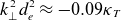 \begin{equation} k_\perp ^2d_{e}^2 \approx -0.09\kappa _T \end{equation}
at large $\kappa _T$
. On this boundary, the MDM solution and its complex conjugate collapse into a repeated root of (3.6), which, to the right of the boundary, splits into two purely real solutions. There is an ambiguity as to which of these should be thought of as the continuation of the MDM, so we have omitted that part of the plot. A similar issue occurs below
$\kappa _T$
. On this boundary, the MDM solution and its complex conjugate collapse into a repeated root of (3.6), which, to the right of the boundary, splits into two purely real solutions. There is an ambiguity as to which of these should be thought of as the continuation of the MDM, so we have omitted that part of the plot. A similar issue occurs below $k_{\perp \text{,min}}^2d_{e}^2$
, and so we have left that part of the plot empty as well. There are no unstable solutions in either of these regions, whether continuously connected to the MDM solution or not. We shall continue the discussion of the MDM solution in the complex plane in § 3.2.3.
$k_{\perp \text{,min}}^2d_{e}^2$
, and so we have left that part of the plot empty as well. There are no unstable solutions in either of these regions, whether continuously connected to the MDM solution or not. We shall continue the discussion of the MDM solution in the complex plane in § 3.2.3.
A characteristic feature of the MDM is that the sign of its real frequency is not given by either $\omega _{T{e}}$
or
$\omega _{T{e}}$
or $\omega _{\text{d}e}$
. The mode can propagate in either the electron (
$\omega _{\text{d}e}$
. The mode can propagate in either the electron ( $\text{Re} \: \omega /\omega _{T{e}} \gt 0$
) or the ion (
$\text{Re} \: \omega /\omega _{T{e}} \gt 0$
) or the ion ( $\text{Re} \: \omega /\omega _{T{e}} \lt 0$
) diamagnetic direction, depending on the size, but not the sign, of the temperature gradient. In contrast, the electrostatic cETG instability can be understood as a destabilised drift wave whose phase velocity is always in the electron diamagnetic direction. This variability of the direction of poloidal propagation of the MDM is not entirely surprising. Indeed, a defining property of the good magnetic curvature is that the magnetic drifts oppose the diamagnetic drifts that arise from the equilibrium gradients. Therefore, both poloidal directions can be associated with one of the electron drifts. In the strongly driven limit
$\text{Re} \: \omega /\omega _{T{e}} \lt 0$
) diamagnetic direction, depending on the size, but not the sign, of the temperature gradient. In contrast, the electrostatic cETG instability can be understood as a destabilised drift wave whose phase velocity is always in the electron diamagnetic direction. This variability of the direction of poloidal propagation of the MDM is not entirely surprising. Indeed, a defining property of the good magnetic curvature is that the magnetic drifts oppose the diamagnetic drifts that arise from the equilibrium gradients. Therefore, both poloidal directions can be associated with one of the electron drifts. In the strongly driven limit $\left \rvert {\kappa _T}\right \rvert \to \infty$
, the maximum growth rate is attained at
$\left \rvert {\kappa _T}\right \rvert \to \infty$
, the maximum growth rate is attained at
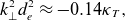 \begin{equation} k_\perp ^2d_{e}^2 \approx -0.14\kappa _T, \end{equation}
where the complex frequency is given by
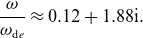 \begin{equation} \frac {\omega }{\omega _{\text{d}e}} \approx 0.12 + 1.88\textrm {i}. \end{equation}
Thus, the phase velocity of the fastest-growing, strongly driven MDM is in the direction of the electron magnetic drifts, which is opposite to that of the electron diamagnetic flows.
There is, however, an important physical distinction between the magnetic drifts, caused by the magnetic-field gradients, and the diamagnetic ones, resulting from the inhomogeneous plasma equilibrium. The magnetic drifts are ‘real’ particle drifts, while the diamagnetic ones are only ‘apparent’ drifts, in the sense that they are not associated with the motion of individual particles. Thus, resonant effects (like Landau damping) are possible only with the magnetic drifts. However, the MDM is not a resonant instability. This is manifestly true as the mode can propagate in either direction relative to the poloidal particle motion (given by the magnetic drift). We discuss this further in § 3.2.3, where we show that the MDM root of the dispersion relation (3.6) is continuously connected to a non-resonant, undamped magnetic drift wave propagating against the magnetic drifts.
Finally, unlike cETG, the MDM is not a fluid instability since its complex frequency always satisfies $\omega \lesssim \omega _{\text{d}e}$
. Consequently, the MDM does not have a fluid counterpart and cannot be captured by a low-order truncation of the infinite hierarchy of fluid moments of electron drift-kinetic equation. This is discussed further in Appendix E.
$\omega \lesssim \omega _{\text{d}e}$
. Consequently, the MDM does not have a fluid counterpart and cannot be captured by a low-order truncation of the infinite hierarchy of fluid moments of electron drift-kinetic equation. This is discussed further in Appendix E.
3.2.3. Physical ingredients and complex-plane behaviour of the MDM
Since the MDM is neither resonant nor ‘fluidisable’, it is difficult to come up with a convincing physical picture of the feedback mechanism that underpins this instability. Let us explore how the root of the dispersion relation (3.6) that corresponds to the MDM connects to other known low- $\beta$
modes. In figure 4, we show the complex-plane trajectory of the roots of (3.6) as functions of the temperature gradient
$\beta$
modes. In figure 4, we show the complex-plane trajectory of the roots of (3.6) as functions of the temperature gradient $\kappa _T$
.Footnote
9
$\kappa _T$
.Footnote
9
A visualisation of the motion of the MDM solution to (3.6) in the complex $\omega$
plane as a function of
$\omega$
plane as a function of $\kappa _T$
. The colours indicate the value of
$\kappa _T$
. The colours indicate the value of $\kappa _T$
, as indicated in the colour bar on the right-hand side. The zigzagging black line is the branch cut of the square root in (3.6).
$\kappa _T$
, as indicated in the colour bar on the right-hand side. The zigzagging black line is the branch cut of the square root in (3.6).
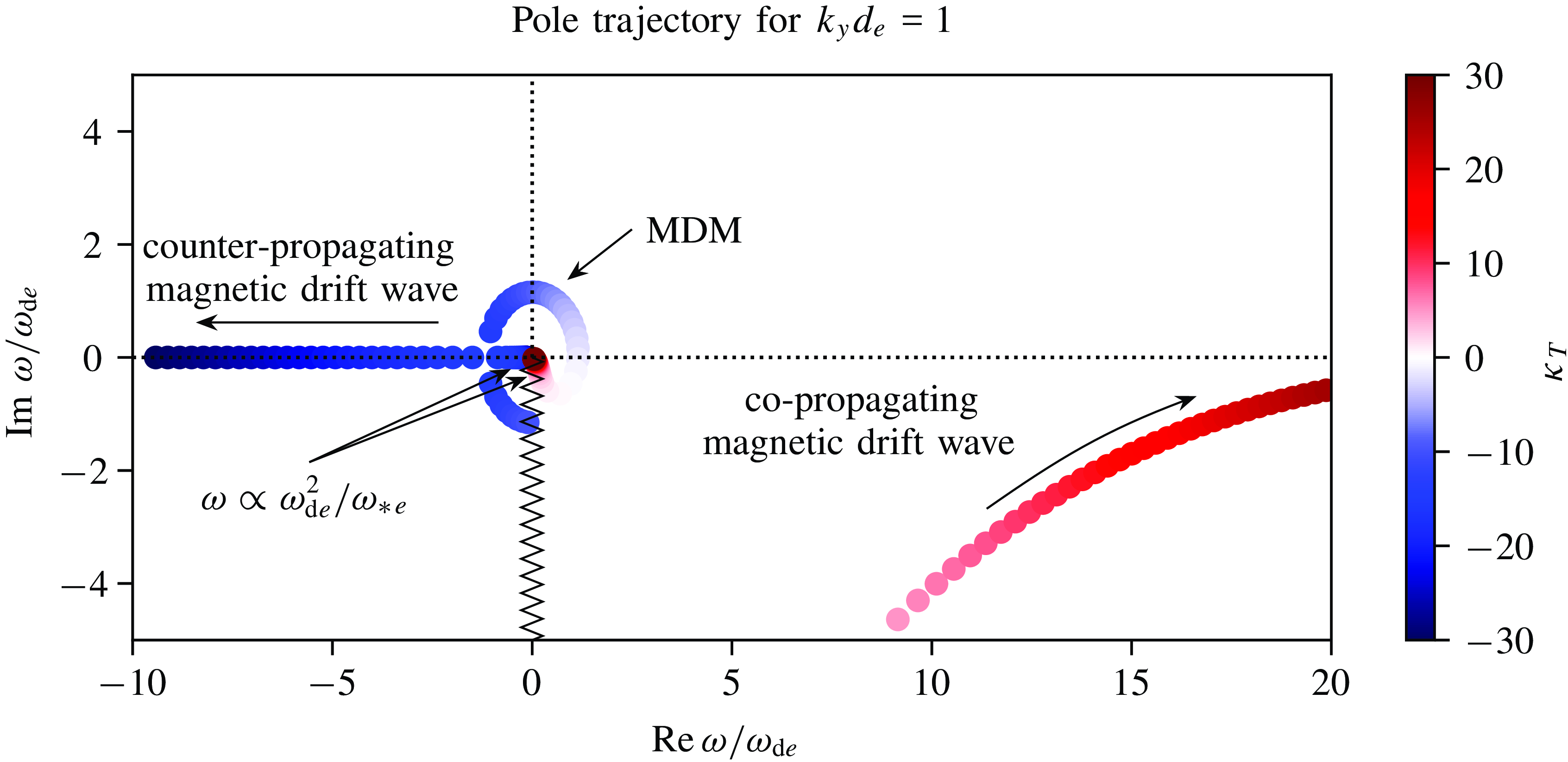
At large temperature gradients, viz. $\left \rvert {\kappa _T}\right \rvert \gg 1$
, there are two weakly damped (or undamped) solutions. The first one satisfies
$\left \rvert {\kappa _T}\right \rvert \gg 1$
, there are two weakly damped (or undamped) solutions. The first one satisfies $\omega \sim \omega _{T{e}} \gg \omega _{\text{d}e}$
for
$\omega \sim \omega _{T{e}} \gg \omega _{\text{d}e}$
for $\left \rvert {\kappa _T}\right \rvert \gg 1$
and can be identified as the magnetic drift wave (Adkins et al. Reference Adkins, Schekochihin, Ivanov and Roach2022; Chandran & Schekochihin Reference Chandran and Schekochihin2024). As
$\left \rvert {\kappa _T}\right \rvert \gg 1$
and can be identified as the magnetic drift wave (Adkins et al. Reference Adkins, Schekochihin, Ivanov and Roach2022; Chandran & Schekochihin Reference Chandran and Schekochihin2024). As $\omega \gg \omega _{\text{d}e}$
, this wave is a ‘fluid’ mode, and, as expected, can be described using only low-order moments of the distribution function. Setting
$\omega \gg \omega _{\text{d}e}$
, this wave is a ‘fluid’ mode, and, as expected, can be described using only low-order moments of the distribution function. Setting ${L}_{B}^{-1} = 0$
, we take the
${L}_{B}^{-1} = 0$
, we take the $v_\parallel$
moment of the electron drift-kinetic equation (C.16) to find the electron-momentum equation
$v_\parallel$
moment of the electron drift-kinetic equation (C.16) to find the electron-momentum equation
 \begin{equation} {n_{e}}m_{e}\frac {\partial {u_{\parallel {e}}}}{\partial {t}} = -\frac {\delta \boldsymbol{B}_\perp }{B}\boldsymbol{\cdot }{\boldsymbol{\nabla }} p_{e} -e{n_{e}} \delta E_\parallel . \end{equation}
Physically, (3.19) expresses the change in parallel momentum of the electrons as a result of the inductive parallel electric field (note that since $k_\parallel =0$
,
$k_\parallel =0$
, $\delta E_\parallel$
has no electrostatic part)
$\delta E_\parallel$
has no electrostatic part)
 \begin{equation} \delta E_\parallel = -\frac {1}{c}\frac {\partial {\delta A_\parallel }}{\partial {t}} \end{equation}
and the equilibrium pressure gradient along the perturbed field line
 \begin{equation} -\frac {\delta \boldsymbol{B}_\perp }{B} \boldsymbol{\cdot } {\boldsymbol{\nabla }} p_{e} = \left (\frac {p_{e}}{L_{n_{e}}} + \frac {p_{e}}{L_{T_{e}}}\right )\frac {\delta B_x}{B} \propto \left (\omega _{*{e}} + \omega _{T{e}}\right )\frac {\partial {\delta A_\parallel }}{\partial {y}}. \end{equation}
Combining (3.19) and the parallel Ampère’s law (C.14), we obtain a purely oscillating mode with frequency
 \begin{equation} \omega = \frac {\omega _{*{e}} + \omega _{T{e}}}{1 + k_\perp ^2d_{e}^2}. \end{equation}
With the inclusion of finite but small magnetic drifts, the fate of the magnetic drift wave is determined by the relative sign of $\omega _{\text{d}e}$
and the diamagnetic frequencies
$\omega _{\text{d}e}$
and the diamagnetic frequencies $\omega _{*{e}}$
and
$\omega _{*{e}}$
and $\omega _{T{e}}$
. If the magnetic drifts are aligned with the direction of propagation, i.e. if
$\omega _{T{e}}$
. If the magnetic drifts are aligned with the direction of propagation, i.e. if $\kappa _T \gt 0$
, then the wave experiences a form of Landau damping due to the resonance between the poloidal drift of the electrons and the phase velocity of the wave.Footnote
10
In contrast, if the magnetic drifts are opposite to the direction of propagation of the magnetic drift wave, i.e. if
$\kappa _T \gt 0$
, then the wave experiences a form of Landau damping due to the resonance between the poloidal drift of the electrons and the phase velocity of the wave.Footnote
10
In contrast, if the magnetic drifts are opposite to the direction of propagation of the magnetic drift wave, i.e. if $\kappa _T \lt 0$
, no resonance is possible and the wave remains undamped. The difference in behaviour of copropagating and counter-propagating drift waves is evident in figure 4. There, the dark red points show the behaviour of the solution as
$\kappa _T \lt 0$
, no resonance is possible and the wave remains undamped. The difference in behaviour of copropagating and counter-propagating drift waves is evident in figure 4. There, the dark red points show the behaviour of the solution as $\kappa _T \to +\infty$
, where the solution converges to a damped, copropagating magnetic drift wave. In contrast, as
$\kappa _T \to +\infty$
, where the solution converges to a damped, copropagating magnetic drift wave. In contrast, as $\kappa _T \to -\infty$
(dark blue points), the solution is an undamped, counter-propagating magnetic drift wave.
$\kappa _T \to -\infty$
(dark blue points), the solution is an undamped, counter-propagating magnetic drift wave.
Apart from the magnetic drift wave (3.22), a small but finite magnetic-drift frequency $\left \rvert {\omega _{\text{d}e}}\right \rvert \ll \left \rvert {\omega _{T{e}}}\right \rvert$
gives rise to another wave whose frequency satisfies
$\left \rvert {\omega _{\text{d}e}}\right \rvert \ll \left \rvert {\omega _{T{e}}}\right \rvert$
gives rise to another wave whose frequency satisfies
 \begin{equation} \omega \sim \frac {(k_\perp ^2 - k_{\perp \text{,min}}^2)d_{e}^2\omega _{\text{d}e}^2}{\omega _{T{e}}}. \end{equation}
This mode is purely oscillatory if $\kappa _T \lt 0$
and damped if
$\kappa _T \lt 0$
and damped if $\kappa _T \gt 0$
due to the resonance with the magnetic drifts. Unlike the magnetic drift wave, the wave (3.23) cannot be described in terms of low-order moments as
$\kappa _T \gt 0$
due to the resonance with the magnetic drifts. Unlike the magnetic drift wave, the wave (3.23) cannot be described in terms of low-order moments as $\omega \ll \omega _{\text{d}e}$
. As
$\omega \ll \omega _{\text{d}e}$
. As $\kappa _T$
is increased from
$\kappa _T$
is increased from $-\infty$
towards zero, the magnetic drift waves (3.22) and (3.23) are both undamped and counter-propagating (relative to the magnetic drift) if
$-\infty$
towards zero, the magnetic drift waves (3.22) and (3.23) are both undamped and counter-propagating (relative to the magnetic drift) if $k_\perp ^2d_{e}^2 \gt k_{\perp \text{,min}}^2d_{e}^2$
. The MDM appears when their frequencies meet at some finite, negative
$k_\perp ^2d_{e}^2 \gt k_{\perp \text{,min}}^2d_{e}^2$
. The MDM appears when their frequencies meet at some finite, negative $\kappa _T$
. This value of
$\kappa _T$
. This value of $\kappa _T$
lies on the lower stability boundary in figure 3. As
$\kappa _T$
lies on the lower stability boundary in figure 3. As $\kappa _T$
increases, the MDM solution changes from counter-propagating (
$\kappa _T$
increases, the MDM solution changes from counter-propagating ( $\omega \lt 0$
) to copropagating (
$\omega \lt 0$
) to copropagating ( $\omega \gt 0$
), before crossing the real line again when
$\omega \gt 0$
), before crossing the real line again when $\kappa _T$
crosses the upper stability boundary in figure 3 at some
$\kappa _T$
crosses the upper stability boundary in figure 3 at some $\kappa _T \lt 0$
. Increasing
$\kappa _T \lt 0$
. Increasing $\kappa _T$
further to
$\kappa _T$
further to $+\infty$
connects the MDM solution to the copropagating mode satisfying (3.23), which is resonantly damped. As
$+\infty$
connects the MDM solution to the copropagating mode satisfying (3.23), which is resonantly damped. As $\kappa _T \to +\infty$
, there is also a copropagating magnetic drift wave. This wave, unlike its counter-propagating part, is not connected to the MDM solution and experiences finite damping due to a resonance with the magnetic drifts. Figure 4 shows the motion of the modes in the complex
$\kappa _T \to +\infty$
, there is also a copropagating magnetic drift wave. This wave, unlike its counter-propagating part, is not connected to the MDM solution and experiences finite damping due to a resonance with the magnetic drifts. Figure 4 shows the motion of the modes in the complex $\omega$
plane as a function of
$\omega$
plane as a function of $\kappa _T$
.
$\kappa _T$
.
Finally, we can gain more insight into the MDM by artificially removing terms from the equations. While unphysical, this can help us understand how the feedback mechanism works and what the minimal set of ingredients for this instability is. We find that removing the ${\boldsymbol{\nabla }} B$
drifts, viz. the magnetic drifts proportional to
${\boldsymbol{\nabla }} B$
drifts, viz. the magnetic drifts proportional to $v_\perp ^2$
, does very little to change the behaviour of the instability. Even in their absence, we find a mode with the same qualitative behaviour as the MDM. However, removing the curvature drifts eliminates the instability completely. This is in stark contrast with the curvature-driven ETG instability discussed in § 3.2.1, which is qualitatively unchanged if either (but not both!) of the drifts is removed. In the strongly driven regime, its growth rate simply reduces by a factor of the square root of two if one of the drifts is not present. We outline these calculations in Appendix G.1. Then, in Appendix G.2, we abandon the Maxwellian equilibrium entirely and consider a greatly simplified
$v_\perp ^2$
, does very little to change the behaviour of the instability. Even in their absence, we find a mode with the same qualitative behaviour as the MDM. However, removing the curvature drifts eliminates the instability completely. This is in stark contrast with the curvature-driven ETG instability discussed in § 3.2.1, which is qualitatively unchanged if either (but not both!) of the drifts is removed. In the strongly driven regime, its growth rate simply reduces by a factor of the square root of two if one of the drifts is not present. We outline these calculations in Appendix G.1. Then, in Appendix G.2, we abandon the Maxwellian equilibrium entirely and consider a greatly simplified $F_{e}$
made up of two infinitely narrow (in
$F_{e}$
made up of two infinitely narrow (in $v_\parallel$
) colliding beams that allows us to obtain qualitatively the same mode. That model suggests that the stabilisation at
$v_\parallel$
) colliding beams that allows us to obtain qualitatively the same mode. That model suggests that the stabilisation at $\text{Re}\:\omega \gt 0$
, viz. the upper stability boundary in figure 3, is a consequence of the Landau-like damping of the copropagating MDM.
$\text{Re}\:\omega \gt 0$
, viz. the upper stability boundary in figure 3, is a consequence of the Landau-like damping of the copropagating MDM.
3.3. Magnetic-drift modes in three dimensions
Restoring finite $k_\parallel$
requires solving the three-dimensional dispersion relation (D.22). Figure 5 is a visualisation of such a solution for three-dimensional fluctuations in the
$k_\parallel$
requires solving the three-dimensional dispersion relation (D.22). Figure 5 is a visualisation of such a solution for three-dimensional fluctuations in the $Z$
-pinch geometry as a function of
$Z$
-pinch geometry as a function of $k_\perp ^2d_{e}^2$
and
$k_\perp ^2d_{e}^2$
and $\kappa _T$
. We see that finite
$\kappa _T$
. We see that finite $k_\parallel$
stabilises the MDM at large scales and low temperature gradients, but the instability survives at large gradients.
$k_\parallel$
stabilises the MDM at large scales and low temperature gradients, but the instability survives at large gradients.
The MDM growth rate for $\kappa _n = -1$
(as in figure 3) for four different values of
$\kappa _n = -1$
(as in figure 3) for four different values of $k_\parallel$
as indicated in the title of each panel. Note that (3.1) and (3.2) imply that the parallel wavenumber always satisfies
$k_\parallel$
as indicated in the title of each panel. Note that (3.1) and (3.2) imply that the parallel wavenumber always satisfies $k_\parallel {L_B} \sim \sqrt {\beta _{e}}$
. Unlike figure 3, we are only showing the regions of positive growth rate.
$k_\parallel {L_B} \sim \sqrt {\beta _{e}}$
. Unlike figure 3, we are only showing the regions of positive growth rate.
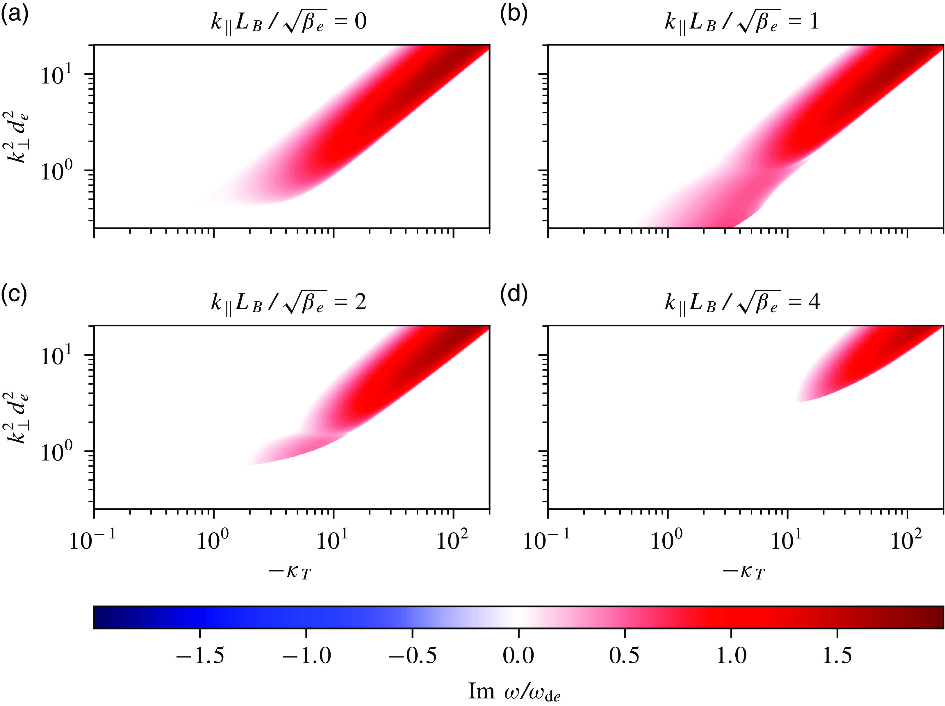
We can make the following heuristic argument about the size of $k_\parallel$
that will be sufficient to affect the MDM. Taking the strongly driven case
$k_\parallel$
that will be sufficient to affect the MDM. Taking the strongly driven case $\omega _{T{e}} \gg \omega _{\text{d}e}$
(or, equivalently,
$\omega _{T{e}} \gg \omega _{\text{d}e}$
(or, equivalently, $\kappa _T \gg 1$
), we expect that three-dimensional effects will not introduce any qualitative changes to the mode if
$\kappa _T \gg 1$
), we expect that three-dimensional effects will not introduce any qualitative changes to the mode if
 \begin{equation} k_\parallel v_{\text{th}{e}} \lesssim \omega _{\text{d}e} \quad \Rightarrow \quad k_\parallel {L_B} \lesssim k_y\rho _{e}. \end{equation}
By (3.15) and (3.16), the MDM exists at scales $k_\perp ^2d_{e}^2 \sim \kappa _T$
, so (3.24) implies
$k_\perp ^2d_{e}^2 \sim \kappa _T$
, so (3.24) implies
 \begin{equation} k_\parallel \lesssim \sqrt {\frac {\beta _{e}}{{L_B}L_{T_{e}}}}. \end{equation}
Since the MDM is destabilised only in the good-curvature region, the parallel extent of the mode is limited by the connection length between the inboard and outboard side of the device, viz.
 \begin{equation} k_\parallel \gtrsim \frac {1}{qR}, \end{equation}
where $q$
is the safety factor and
$q$
is the safety factor and $R\sim {L_B}$
is the major radius. Therefore, we expect the MDM to be destabilised in toroidal geometry if
$R\sim {L_B}$
is the major radius. Therefore, we expect the MDM to be destabilised in toroidal geometry if
 \begin{equation} \frac {\beta _{e}{L_B}}{L_{T_{e}}} \gtrsim \frac {1}{q^2}, \end{equation}
which shows that, for a fixed geometry, steeper temperature gradients and/or higher values of $\beta _{e}$
will trigger the MDM. In (3.27), we neglect order-unity factors that will undoubtedly impact the true condition for MDM destabilisation in toroidal geometry. However, we expect this simple scaling estimate to capture the trend of the MDM threshold as a function of
$\beta _{e}$
will trigger the MDM. In (3.27), we neglect order-unity factors that will undoubtedly impact the true condition for MDM destabilisation in toroidal geometry. However, we expect this simple scaling estimate to capture the trend of the MDM threshold as a function of $\beta _{e}$
and of the temperature gradient.
$\beta _{e}$
and of the temperature gradient.
In addition to the threshold for the MDM, we can make a rough estimate of the expected growth rate and compare it with that of other known instabilities. Recall that both the real and imaginary parts of the frequency of the MDM satisfy $\omega \sim \omega _{\text{d}e}$
. Combining this with the requirement that
$\omega \sim \omega _{\text{d}e}$
. Combining this with the requirement that $k_\perp ^2d_{e}^2 \sim \kappa _T$
, the growth rate of the MDM can be estimated as
$k_\perp ^2d_{e}^2 \sim \kappa _T$
, the growth rate of the MDM can be estimated as
 \begin{equation} \gamma _{\text{MDM}} \sim \frac {\rho _{e} v_{\text{th}{e}} k_y }{{L_B}} \sim \frac {v_{\text{th}{e}}}{\sqrt {{L_B}L_{T_{e}}}}\sqrt {\beta _{e}}. \end{equation}
To put this in the context of more common GK instabilities, let us compare it with the usual estimate for the growth rate of the cITG instability, viz.
 \begin{equation} \gamma _{\text{ITG}} \sim \frac {v_{\text{th}{i}}}{\sqrt {{L_B}L_{T_{i}}}}. \end{equation}
Assuming similar temperature gradients, viz. $L_{T_{i}} \sim L_{T_{e}}$
, we find
$L_{T_{i}} \sim L_{T_{e}}$
, we find
 \begin{equation} \frac {\gamma _{\text{MDM}}}{\gamma _{\text{ITG}}} \sim \sqrt {\frac {\beta _{e}m_{i}}{m_{e}}}, \end{equation}
and so the MDM growth rate is (potentially) larger than the cITG one in any device where $\beta _{e} \gg m_{e}/m_{i}$
.Footnote
11
Of course, (3.28)–(3.30) are very rough estimates that are true only within potentially important factors of order unity. They also fail to consider the possible mitigation of the instabilities due either to neglected linear effects, like toroidal geometry and magnetic shear, or to nonlinear effects, for example suppression of fluctuations as a result of multiscale interactions (Waltz, Candy & Fahey Reference Waltz, Candy and Fahey2007; Candy et al. Reference Candy, Waltz, Fahey and Holland2007; Maeyama et al. Reference Maeyama, Idomura, Watanabe, Nakata, Yagi, Miyato, Ishizawa and Nunami2015, Reference Maeyama, Watanabe, Idomura, Nakata, Ishizawa and Nunami2017; Hardman et al. Reference Hardman, Barnes, Roach and Parra2019, Reference Hardman, Barnes and Roach2020). It is also worth noting that, in electron-scale simulations of GK turbulence, even if present, the MDM is likely to be subdominant to the more common electrostatic ETG instabilities, whose growth rate,
$\beta _{e} \gg m_{e}/m_{i}$
.Footnote
11
Of course, (3.28)–(3.30) are very rough estimates that are true only within potentially important factors of order unity. They also fail to consider the possible mitigation of the instabilities due either to neglected linear effects, like toroidal geometry and magnetic shear, or to nonlinear effects, for example suppression of fluctuations as a result of multiscale interactions (Waltz, Candy & Fahey Reference Waltz, Candy and Fahey2007; Candy et al. Reference Candy, Waltz, Fahey and Holland2007; Maeyama et al. Reference Maeyama, Idomura, Watanabe, Nakata, Yagi, Miyato, Ishizawa and Nunami2015, Reference Maeyama, Watanabe, Idomura, Nakata, Ishizawa and Nunami2017; Hardman et al. Reference Hardman, Barnes, Roach and Parra2019, Reference Hardman, Barnes and Roach2020). It is also worth noting that, in electron-scale simulations of GK turbulence, even if present, the MDM is likely to be subdominant to the more common electrostatic ETG instabilities, whose growth rate,
 \begin{equation} \gamma _{\text{ETG}}\sim \frac {v_{\text{th}{e}}}{\sqrt {{L_B}L_{T_{e}}}}, \end{equation}
is a factor of $\beta _{e}^{-1/2}$
larger than (3.28). While this could make it harder to identify the MDM in linear simulations, its effects may still be crucial for the nonlinear turbulent state because it can drive turbulence in the good-curvature regions where the ETG modes are stable.
$\beta _{e}^{-1/2}$
larger than (3.28). While this could make it harder to identify the MDM in linear simulations, its effects may still be crucial for the nonlinear turbulent state because it can drive turbulence in the good-curvature regions where the ETG modes are stable.
It is likely that what we call the MDM here is, in fact, related to other, already observed good-curvature electromagnetic GK instabilities. The intermediate-wavelength microtearing mode reported by Patel (Reference Patel2021) is an electromagnetic, good-curvature mode with a phase speed in the ion diamagnetic direction. Additionally, Jian et al. (Reference Jian, Holland, Candy, Ding, Belli, Chan, Staebler, Garofalo, Mcclenaghan and Snyder2021) have performed linear and nonlinear GK simulations of high- $\beta$
DIII-D equilibria, wherein they have identified a mode that they call ‘slab microtearing mode’. Linearly, this mode is peaked at the good-curvature side of the device. Nonlinearly, it drives turbulent transport predominantly at the inboard side. Furthermore, they have identified it as a slab mode due to its strong dependence on
$\beta$
DIII-D equilibria, wherein they have identified a mode that they call ‘slab microtearing mode’. Linearly, this mode is peaked at the good-curvature side of the device. Nonlinearly, it drives turbulent transport predominantly at the inboard side. Furthermore, they have identified it as a slab mode due to its strong dependence on $q$
, being destabilised at large values of
$q$
, being destabilised at large values of $q$
, consistent with the analysis leading to (3.27). Both of these examples match the properties of the MDM, at least qualitatively.
$q$
, consistent with the analysis leading to (3.27). Both of these examples match the properties of the MDM, at least qualitatively.
4. Discussion
By considering the conservation laws of the free energy (2.11) and the field invariant (2.16) in GK, we have shown that the localisation of curvature-driven modes to regions of either good or bad magnetic curvature is a necessary condition for instability. In particular, these conservation laws, together with some reasonable assumptions stated in § 2.4, allow us to prove that all electrostatic curvature-driven instabilities are localised to the so-called bad-curvature regions of the plasma, where the local magnetic curvature (2.30) is negative. Consequently, any instabilities in the good-magnetic-curvature region must be electromagnetic. Modulo the assumptions stated in § 2.4, these results are independent of the precise nature of the instability. Note that a similar conclusion regarding the destabilising role of good magnetic curvature for electromagnetic modes was reached by Antonsen, Lane & Ramos (Reference Antonsen, Lane and Ramos1981) who derived conditions for instability based on an MHD-like variational principle. However, they did not provide an explicit example of such an instability and some of their assumptions ordered out the MDM as described in § 3.
The MDM, whose dispersion relation in a low- $\beta$ $Z$
-pinch is given by (3.6), is, as far as the authors are aware, the first example of a simple, analytically derivable, good-curvature instability. In the simple model wherein we have derived it, the MDM exists at perpendicular length scales comparable to the electron skin depth
$Z$
-pinch is given by (3.6), is, as far as the authors are aware, the first example of a simple, analytically derivable, good-curvature instability. In the simple model wherein we have derived it, the MDM exists at perpendicular length scales comparable to the electron skin depth $d_{e}$
and has a growth rate that is
$d_{e}$
and has a growth rate that is $\sqrt {\beta _{e}}$
smaller than that of the cETG instability and much larger than that of the cITG instability in plasmas with
$\sqrt {\beta _{e}}$
smaller than that of the cETG instability and much larger than that of the cITG instability in plasmas with $\beta _{e} \gg m_{e}/m_{i}$
. The fact that it is localised to the good-curvature regions of the equilibrium, where electrostatic modes like cETG and cITG are stable, means that the MDM can be the dominant one there.
$\beta _{e} \gg m_{e}/m_{i}$
. The fact that it is localised to the good-curvature regions of the equilibrium, where electrostatic modes like cETG and cITG are stable, means that the MDM can be the dominant one there.
As discussed in § 3.2.3, the MDM is neither resonant nor fluid. Physically, it arises as a result of the $v_\parallel ^2$
-dependent magnetic-curvature drifts and the parallel streaming of electrons along perturbed field lines. Even though simplified, the model wherein we derived the MDM is a particular asymptotic limit of GK. Therefore, we expect that, under the right conditions (some of which are outlined in § 3.3), the MDM exists in toroidal geometry, too. Indeed, it is likely that is related to some exotic varieties of microtearing mode seen in recent high-
$v_\parallel ^2$
-dependent magnetic-curvature drifts and the parallel streaming of electrons along perturbed field lines. Even though simplified, the model wherein we derived the MDM is a particular asymptotic limit of GK. Therefore, we expect that, under the right conditions (some of which are outlined in § 3.3), the MDM exists in toroidal geometry, too. Indeed, it is likely that is related to some exotic varieties of microtearing mode seen in recent high- $\beta$
GK simulations (Patel Reference Patel2021; Jian et al. Reference Jian, Holland, Candy, Ding, Belli, Chan, Staebler, Garofalo, Mcclenaghan and Snyder2021).
$\beta$
GK simulations (Patel Reference Patel2021; Jian et al. Reference Jian, Holland, Candy, Ding, Belli, Chan, Staebler, Garofalo, Mcclenaghan and Snyder2021).
Given that, both theoretically and experimentally, the vast majority of fusion-plasma research has concentrated on regimes where electrostatic instabilities dominate, it is unsurprising that the community has adopted the term ‘bad curvature’ for the locations where these modes are unstable. However, the pursuit of high- $\beta$
fusion devices, for example STEP (Tholerus et al. Reference Tholerus2024), has opened a Pandora’s box of electromagnetic instabilities and turbulence that challenge conventional intuition and suggest that the performance of such devices could be worse than expected if electromagnetic instabilities are not kept in check (Kennedy et al. Reference Kennedy, Giacomin, Casson, Dickinson, Hornsby, Patel and Roach2023; Giacomin et al. Reference Giacomin, Kennedy, Casson, C. J., Dickinson, Patel and Roach2024). The unstable MDM is likely only one of a class of good-curvature electromagnetic instabilities that are yet to be discovered and understood and whose role in the turbulent transport of high-
$\beta$
fusion devices, for example STEP (Tholerus et al. Reference Tholerus2024), has opened a Pandora’s box of electromagnetic instabilities and turbulence that challenge conventional intuition and suggest that the performance of such devices could be worse than expected if electromagnetic instabilities are not kept in check (Kennedy et al. Reference Kennedy, Giacomin, Casson, Dickinson, Hornsby, Patel and Roach2023; Giacomin et al. Reference Giacomin, Kennedy, Casson, C. J., Dickinson, Patel and Roach2024). The unstable MDM is likely only one of a class of good-curvature electromagnetic instabilities that are yet to be discovered and understood and whose role in the turbulent transport of high- $\beta$
plasmas is currently unknown. For example, good-curvature instabilities driven by trapped particles in non-axisymmetric plasmas could drive turbulence in stellarator equilibria otherwise thought to be (relatively) immune to trapped-particle instabilities (Rodríguez et al. Reference Rodríguez, Helander and Goodman2024. It is thus clear that the study of the good-curvature instabilities, like the MDM, is a fertile field for future work.
$\beta$
plasmas is currently unknown. For example, good-curvature instabilities driven by trapped particles in non-axisymmetric plasmas could drive turbulence in stellarator equilibria otherwise thought to be (relatively) immune to trapped-particle instabilities (Rodríguez et al. Reference Rodríguez, Helander and Goodman2024. It is thus clear that the study of the good-curvature instabilities, like the MDM, is a fertile field for future work.
Acknowledgements
We would like to thank the organisers of the 7th Vlasovia (2024) workshop in Florence, where an early version of this work was first presented. We would also like to thank the organisers of the 15th Plasma Kinetics Working Meeting (2024) and its hosts at the Wolfgang Pauli Institute in Vienna.
Editor Per Helander thanks the referees for their advice in evaluating this article.
Funding
This work was supported by the Engineering and Physical Sciences Research Council (EPSRC) [EP/R034737/1]. The work of A.A.S. was supported in part by the Simons Foundation via a Simons Investigator award. T.A.’s contributions were supported in part by the U.S. Department of Energy under contract number DE-AC02-09CH11466. The United States Government retains a non-exclusive, paid-up, irrevocable, world-wide license to publish or reproduce the published form of this manuscript, or allow others to do so, for United States Government purposes. T.A. also acknowledges the support of the Royal Society Te Apārangi, through Marsden-Fund grant MFP-UOO2221.
Declaration of interests
The authors report no conflict of interest.
Appendix A. Spatial averaging
The average $\langle \!\langle g({\boldsymbol{r}}) \rangle _{\! \perp } \rangle _{\! \psi }$
that appears in the GK conservation laws is a combination of a perpendicular and a flux-surface average. The former, defined as
$\langle \!\langle g({\boldsymbol{r}}) \rangle _{\! \perp } \rangle _{\! \psi }$
that appears in the GK conservation laws is a combination of a perpendicular and a flux-surface average. The former, defined as
 \begin{equation} \left \langle g({\boldsymbol{r}}) \right \rangle _\perp = \int _{S_\lambda } \textrm {d}^{2}{{\boldsymbol{r}}} \, g({\boldsymbol{r}}) \Bigg / \int _{S_\lambda } \textrm {d}^{2}{{\boldsymbol{r}}} \, \end{equation}
is an average in the plane perpendicular to $\boldsymbol{B}$
over an area
$\boldsymbol{B}$
over an area $S_\lambda$
with linear size
$S_\lambda$
with linear size $\lambda$
that is an intermediate length between the microscales associated with the gyroradii and the macroscale of the equilibrium, viz.
$\lambda$
that is an intermediate length between the microscales associated with the gyroradii and the macroscale of the equilibrium, viz.
 \begin{equation} \rho _{s} \ll \lambda \ll L. \end{equation}
By assumption in deriving the GK equation, if $g({\boldsymbol{r}})$
is a fluctuating quantity with perpendicular spatial scales
$g({\boldsymbol{r}})$
is a fluctuating quantity with perpendicular spatial scales
 \begin{equation} \frac {g}{\left \rvert {{\boldsymbol{\nabla }}_\perp g}\right \rvert } \sim \rho _{s}, \end{equation}
then the perpendicular average of $g$
is an equilibrium-like quantity with
$g$
is an equilibrium-like quantity with
 \begin{equation} \frac {\left \langle g \right \rangle _\perp }{\left \rvert {{\boldsymbol{\nabla }}_\perp \left \langle g \right \rangle _\perp }\right \rvert } \sim L. \end{equation}
In other words, the perpendicular average is a kind of coarse-graining that eliminates microscales. As a consequence, averaging a gradient of a fluctuating quantity reduces it by a factor of $\rho _{s}/L$
, viz.
$\rho _{s}/L$
, viz.
 \begin{equation} \frac {\left \rvert {\left \langle {\boldsymbol{\nabla }}_\perp g \right \rangle _\perp }\right \rvert }{\left \rvert {{\boldsymbol{\nabla }}_\perp g}\right \rvert } \sim \frac {\rho _{s}}{L} \ll 1. \end{equation}
The flux-surface average is defined as
 \begin{equation} \left \langle g({\boldsymbol{r}}) \right \rangle _\psi \equiv \lim _{\Delta \psi \to 0} \left [\int _{\Delta V(\psi )} \textrm {d}^{3} {{\boldsymbol{r}}}\, g({\boldsymbol{r}}) \Bigg / \int _{\Delta V(\psi )} \textrm {d}^{3}{{\boldsymbol{r}}} \,\right ], \end{equation}
where $\Delta V(\psi ) = V(\psi +\Delta \psi ) - V(\psi )$
and
$\Delta V(\psi ) = V(\psi +\Delta \psi ) - V(\psi )$
and $V(\psi )$
is the volume of the flux surface labelled by
$V(\psi )$
is the volume of the flux surface labelled by $\psi$
. The only property of the flux-surface average that we will need is that, for any
$\psi$
. The only property of the flux-surface average that we will need is that, for any $g$
,
$g$
,
 \begin{equation} \left \langle {\boldsymbol{\nabla }} \boldsymbol{\cdot }(\boldsymbol{B} g) \right \rangle _\psi = 0, \end{equation}
which is straightforward to derive using (A.6), the divergence theorem, and the fact that $\boldsymbol{B}\boldsymbol{\cdot }\boldsymbol{n} = 0$
where
$\boldsymbol{B}\boldsymbol{\cdot }\boldsymbol{n} = 0$
where $\boldsymbol{n}$
is the normal vector to the flux surface (Abel et al. Reference Abel, Plunk, Wang, Barnes, Cowley, Dorland and Schekochihin2013).
$\boldsymbol{n}$
is the normal vector to the flux surface (Abel et al. Reference Abel, Plunk, Wang, Barnes, Cowley, Dorland and Schekochihin2013).
A.1 Ballooning modes and local GK
Following Connor et al. (Reference Connor, Hastie and Taylor1978), we can represent any fluctuating quantity $g({\boldsymbol{r}})$
associated with a linear mode that satisfies (2.1) as
$g({\boldsymbol{r}})$
associated with a linear mode that satisfies (2.1) as
 \begin{equation} g({\boldsymbol{r}}) = \sum _{p = -\infty }^{+\infty } \hat {g}(\psi , \theta + 2\pi p) \textrm {e}^{\textrm {i} S(\psi , \theta + 2\pi p, \varphi )} + \text{c.c.}, \end{equation}
where the fast (viz. on the scale of $\rho _{s}$
) variation across the magnetic field lines is captured entirely by the eikonal
$\rho _{s}$
) variation across the magnetic field lines is captured entirely by the eikonal $S$
and
$S$
and $\hat {g}$
varies slowly (viz. on the equilibrium length scale
$\hat {g}$
varies slowly (viz. on the equilibrium length scale $L$
) as a function of the flux-surface label
$L$
) as a function of the flux-surface label $\psi$
. The eikonal is expressed as
$\psi$
. The eikonal is expressed as
 \begin{equation} S(\psi , \theta , \varphi ) = n(q\theta - \varphi ) + S_\psi (\psi ), \end{equation}
where $\varphi$
,
$\varphi$
, $q$
and
$q$
and $\theta$
are defined in § 2.2;
$\theta$
are defined in § 2.2; $n$
is the toroidal wavenumber;
$n$
is the toroidal wavenumber; $q(\psi )$
is the safety factor;
$q(\psi )$
is the safety factor; $\psi$
is the flux-surface label (typically, the poloidal flux). Since the perpendicular average (A.1) eliminates modes with fast perpendicular variation,
$\psi$
is the flux-surface label (typically, the poloidal flux). Since the perpendicular average (A.1) eliminates modes with fast perpendicular variation,
 \begin{equation} \left \langle f({\boldsymbol{r}}) g ({\boldsymbol{r}}) \right \rangle _\perp = 2\text{Re}\sum _{p = -\infty }^{+\infty } \hat {f}(\psi , \theta + 2\pi p)\hat {g}^*(\psi , \theta + 2\pi p) \end{equation}
for any two quantities $f({\boldsymbol{r}})$
and
$f({\boldsymbol{r}})$
and $g({\boldsymbol{r}})$
expressed as (A.8).Footnote
12
Flux-surface-averaging (A.10), we find
$g({\boldsymbol{r}})$
expressed as (A.8).Footnote
12
Flux-surface-averaging (A.10), we find
 \begin{align} \langle \!\langle f({\boldsymbol{r}})g({\boldsymbol{r}}) \rangle _{\! \perp } \rangle _{\! \psi } &= 2\text{Re} \!\sum _{p = -\infty }^{+\infty } \lim _{\Delta \psi \to 0} \frac {1}{\Delta V(\psi )} \int _{\Delta V(\psi )} \textrm {d}^{3}{{\boldsymbol{r}}} \, \hat {f}(\psi , \theta + 2\pi p)\hat {g}^*(\psi , \theta + 2\pi p) \nonumber \\ &= 2\text{Re}\! \sum _{p = -\infty }^{+\infty } \lim _{\Delta \psi \to 0} \frac {1}{\Delta V(\psi )}\! \int _{\Delta V(\psi )}\!\! \frac {\textrm {d} \varphi \textrm {d} \theta \textrm {d} \psi }{\mathcal{J}} \hat {f}(\psi , \theta {\kern-1pt}+{\kern-1pt} 2\pi p)\hat {g}^*(\psi , \theta {\kern-1pt}+{\kern-1pt} 2\pi p) \nonumber \\ &= 2\text{Re}\! \sum _{p = -\infty }^{+\infty } \lim _{\Delta \psi \to 0} \frac {\Delta \psi }{\Delta V(\psi )}\! \int _0^{2\pi }\!\! \textrm {d} \varphi\!\! \int _0^{2\pi }\! \frac {\textrm {d} \theta }{\mathcal{J}} \hat {f}(\psi , \theta + 2\pi p)\hat {g}^*(\psi , \theta + 2\pi p) \nonumber \\ &= 2\text{Re} \left \langle \hat {f}(\psi , \theta )\hat {g}^*(\psi , \theta )\right \rangle _ \parallel , \end{align}
where we have defined the parallel average of any function $\hat {f}(\psi , \theta )$
to be
$\hat {f}(\psi , \theta )$
to be
 \begin{equation} \left \langle \hat {f}(\psi , \theta )\right \rangle _ \parallel \equiv \int _{-\infty }^{+\infty } \frac {\textrm {d} \theta }{\mathcal{J}} \hat {f}(\psi , \theta ) \Bigg / \int _{0}^{2\pi } \frac {\textrm {d} \theta }{\mathcal{J}}. \end{equation}
In the above, $\mathcal{J} = ({\boldsymbol{\nabla }} \varphi \times {\boldsymbol{\nabla }} \theta )\boldsymbol{\cdot } {\boldsymbol{\nabla }} \psi$
is the Jacobian, and we have used the fact that, in axisymmetric geometry,
$\mathcal{J} = ({\boldsymbol{\nabla }} \varphi \times {\boldsymbol{\nabla }} \theta )\boldsymbol{\cdot } {\boldsymbol{\nabla }} \psi$
is the Jacobian, and we have used the fact that, in axisymmetric geometry, $\mathcal{J}$
is independent of
$\mathcal{J}$
is independent of $\varphi$
at fixed
$\varphi$
at fixed $\theta$
and
$\theta$
and $\psi$
.
$\psi$
.
Alternatively, in a GK flux tube with local coordinates $(x, y, z)$
and periodic boundary conditions across the field lines, we can Fourier transform in
$(x, y, z)$
and periodic boundary conditions across the field lines, we can Fourier transform in $x$
and
$x$
and $y$
as in (2.18). In such a flux tube, we define
$y$
as in (2.18). In such a flux tube, we define $\langle \!\langle . \rangle _{\! \perp } \rangle _{\! \psi }$
as the average over the entire flux tube
$\langle \!\langle . \rangle _{\! \perp } \rangle _{\! \psi }$
as the average over the entire flux tube
 \begin{equation} \langle \langle g({\boldsymbol{r}}) \rangle _{\! \perp } \rangle _{\! \psi } = \frac {1}{V_1} {\int \textrm {d}^{3} \boldsymbol{r}} g({\boldsymbol{r}}) \end{equation}
where $V_1$
is an appropriate normalising volume. Then, using (2.18) and (A.13), we find that, for two flux-tube quantities
$V_1$
is an appropriate normalising volume. Then, using (2.18) and (A.13), we find that, for two flux-tube quantities $f({\boldsymbol{r}})$
and
$f({\boldsymbol{r}})$
and $g({\boldsymbol{r}})$
,
$g({\boldsymbol{r}})$
,
 \begin{equation} \langle \langle f({\boldsymbol{r}})g({\boldsymbol{r}}) \rangle _{\! \perp } \rangle _{\! \psi } = \frac {S_\perp }{V_1}\sum _{{\boldsymbol{k}}_\perp } \int _{-\infty }^{+\infty } \frac {\textrm {d} z}{\mathcal{J}} f_{{\boldsymbol{k}}_\perp } g_{{\boldsymbol{k}}_\perp }^*, \end{equation}
where $S_\perp = \int \textrm {d} x \textrm {d} y$
is the perpendicular surface area of the flux tube and
$S_\perp = \int \textrm {d} x \textrm {d} y$
is the perpendicular surface area of the flux tube and $\mathcal{J} = ({\boldsymbol{\nabla }} x \times {\boldsymbol{\nabla }} y)\boldsymbol{\cdot } {\boldsymbol{\nabla }} z$
is the Jacobian of the flux-tube coordinate system. Note that
$\mathcal{J} = ({\boldsymbol{\nabla }} x \times {\boldsymbol{\nabla }} y)\boldsymbol{\cdot } {\boldsymbol{\nabla }} z$
is the Jacobian of the flux-tube coordinate system. Note that $\mathcal{J}$
is a function only of
$\mathcal{J}$
is a function only of $z$
since it is an equilibrium quantity whose length scale of variation
$z$
since it is an equilibrium quantity whose length scale of variation $L$
is much larger than the perpendicular extent of the flux tube (which is comparable to
$L$
is much larger than the perpendicular extent of the flux tube (which is comparable to $\rho _{s}$
). The above is equivalent to summing a spectrum of ballooning modes and averaging as per (A.12) if we define the parallel average in the flux tube as
$\rho _{s}$
). The above is equivalent to summing a spectrum of ballooning modes and averaging as per (A.12) if we define the parallel average in the flux tube as
 \begin{equation} \left \langle g\right \rangle _ \parallel \equiv \frac {S_\perp }{V_1} \int _{-\infty }^{+\infty } \frac {\textrm {d} z}{\mathcal{J}} g. \end{equation}
Note that the choice of $x \propto \psi$
and
$x \propto \psi$
and $y \propto \alpha$
that we made in § 2.1, together with
$y \propto \alpha$
that we made in § 2.1, together with $z = \theta$
implies
$z = \theta$
implies $\mathcal{J} \propto ({\boldsymbol{\nabla }} \varphi \times {\boldsymbol{\nabla }} \theta )\boldsymbol{\cdot } {\boldsymbol{\nabla }} \psi$
. In this case, the normalising volume is
$\mathcal{J} \propto ({\boldsymbol{\nabla }} \varphi \times {\boldsymbol{\nabla }} \theta )\boldsymbol{\cdot } {\boldsymbol{\nabla }} \psi$
. In this case, the normalising volume is
 \begin{equation} V_1 = \int _{\theta \in (0, 2\pi )} \textrm {d}^{3} {{\boldsymbol{r}}}\, = S_\perp \int _{0}^{2\pi } \frac {\textrm {d} \theta }{\mathcal{J}}, \end{equation}
i.e. it is the volume of the flux tube per $2\pi$
period in
$2\pi$
period in $\theta$
, and (A.15) becomes
$\theta$
, and (A.15) becomes
 \begin{equation} \left \langle g\right \rangle _ \parallel = \int _{-\infty }^{+\infty } \frac {\textrm {d} \theta }{\mathcal{J}} g \Bigg / \int _{0}^{2\pi } \frac {\textrm {d} \theta }{\mathcal{J}}. \end{equation}
Thus, (A.12) and (A.15) do indeed represent the same average.
More details on the correspondence between the ballooning representation and the local flux tubes can be found in Beer et al. (Reference Beer, Cowley and Hammett1995).
Appendix B. Gyrokinetic conservations laws
B.1 Alternative expression for
$W$

Let us show that the free energy (2.10) can also be expressed as
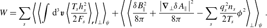 \begin{equation} W = \sum _s\left \langle \,\left \langle {\int \textrm {d}^{3} \boldsymbol{v}\left \langle \frac {T_{s}h_{s}^2}{2F_{s}} \right \rangle _{\boldsymbol{r}}} \right \rangle _{\! \perp } \right \rangle _{\! \psi } + \left \langle \,\left \langle {\frac {\delta B_\parallel ^2}{8\pi } + \frac {\left \rvert {{\boldsymbol{\nabla }}_\perp \delta A_\parallel }\right \rvert ^2}{8\pi } - \sum _s \frac {q_{s}^2n_{s}}{2T_{s}}\phi ^2} \right \rangle _{\! \perp } \right \rangle _{\! \psi }. \end{equation}
This is a standard result (see, e.g. Abel et al. Reference Abel, Plunk, Wang, Barnes, Cowley, Dorland and Schekochihin2013), but we prove it here for completeness. Using (2.3), we find
 \begin{equation} \sum _s \left \langle \,\left \langle {\int \textrm {d}^{3} \boldsymbol{v} \frac {T_{s}\delta f_{s}^2}{2F_{s}}} \right \rangle _{\! \perp } \right \rangle _{\! \psi } = \sum _s \left \langle \,\left \langle {\int \textrm {d}^{3} \boldsymbol{v} \left \langle \frac {T_{s}h_{s}^2}{2F_{s}} - q_{s} \phi h_{s} + \frac {q_{s}^2\phi ^2}{2T_{s}}F_{s} \right \rangle _{\boldsymbol{r}}} \right \rangle _{\! \perp } \right \rangle _{\! \psi }, \end{equation}
where the overall gyroaverage $\left \langle . \right \rangle _{\boldsymbol{r}}$
signifies that the
$\left \langle . \right \rangle _{\boldsymbol{r}}$
signifies that the $\textrm {d}^{3} \boldsymbol{v}\,$
integral is performed with
$\textrm {d}^{3} \boldsymbol{v}\,$
integral is performed with $\boldsymbol{r}$
held constant. By (2.7), we have
$\boldsymbol{r}$
held constant. By (2.7), we have
 \begin{equation} \sum _s \left \langle \,\left \langle {\int \textrm {d}^{3} \boldsymbol{v} \left \langle q_{s} \phi h_{s} \right \rangle _{\boldsymbol{r}}} \right \rangle _{\! \perp } \right \rangle _{\! \psi } = \sum _s \left \langle \,\left \langle {\int \textrm {d}^{3} \boldsymbol{v}\, q_{s}\phi \left \langle h_{s} \right \rangle _{\boldsymbol{r}}} \right \rangle _{\! \perp } \right \rangle _{\! \psi } = \sum _s \left \langle \,\left \langle {\frac {q_{s}^2n_{s}}{T_{s}}\phi ^2} \right \rangle _{\! \perp } \right \rangle _{\! \psi }, \end{equation}
and so (B.2) becomes
 \begin{equation} \sum _s \left \langle \,\left \langle {\int \textrm {d}^{3} \boldsymbol{v} \frac {T_{s}\delta f_{s}^2}{2F_{s}}} \right \rangle _{\! \perp } \right \rangle _{\! \psi } = \sum _s \left \langle \,\left \langle {\int \textrm {d}^{3} \boldsymbol{v} \left \langle \frac {T_{s}h_{s}^2}{2F_{s}} \right \rangle _{\boldsymbol{r}}} \right \rangle _{\! \perp } \right \rangle _{\! \psi } - \sum _s\left \langle \,\left \langle {\frac {q_{s}^2n_{s}}{2T_{s}}\phi ^2} \right \rangle _{\! \perp } \right \rangle _{\! \psi }. \end{equation}
Finally, using
 \begin{equation} \left \rvert {\delta \boldsymbol{B}}\right \rvert ^2 = \left \rvert {\delta B_\parallel {{\hat {\boldsymbol{b}}}} - {{\hat {\boldsymbol{b}}}} \times {\boldsymbol{\nabla }}_\perp \delta A_\parallel }\right \rvert ^2 = \delta B_\parallel ^2 + \left \rvert {{\boldsymbol{\nabla }}_\perp \delta A_\parallel }\right \rvert ^2, \end{equation}
we obtain (B.1). Note that, in the local limit, (B.1) can be written as
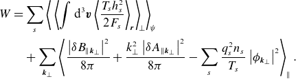 \begin{align} W &= \sum _s\left \langle \,\left \langle {\int \textrm {d}^{3} \boldsymbol{v} \left \langle \frac {T_{s}h_{s}^2}{2F_{s}} \right \rangle _{\boldsymbol{r}}} \right \rangle _{\! \perp } \right \rangle _{\! \psi } \nonumber \\ &\quad +\sum _{{\boldsymbol{k}}_\perp }\left \langle \frac {\left \rvert {\delta {B}_{\parallel {{\boldsymbol{k}}_\perp }}}\right \rvert ^2}{8\pi } + \frac {k_\perp ^2\left \rvert {\delta {A}_{\parallel {{\boldsymbol{k}}_\perp }}}\right \rvert ^2}{8\pi } - \sum _s \frac {q_{s}^2n_{s}}{T_{s}}\left \rvert {{\phi }_{{\boldsymbol{k}}_\perp }}\right \rvert ^2\right \rangle _ \parallel . \end{align}
B.2 Injection terms for
$W$

Here, we derive (2.11) and give explicit formulae for the particle and heat fluxes. To begin, using (2.4), we find
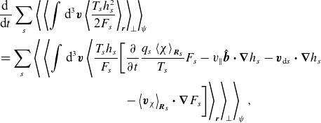 \begin{align} &\frac {\textrm {d}^{}}{\textrm {d}{t}} \sum _s \left \langle \,\left \langle {\int \textrm {d}^{3} \boldsymbol{v} \left \langle \frac {T_{s}h_{s}^2}{2F_{s}} \right \rangle _{\boldsymbol{r}}} \right \rangle _{\! \perp } \right \rangle _{\! \psi } \nonumber \\ &=\sum _s \left \langle \,\left \langle \int \textrm {d}^{3} \boldsymbol{v} \left \langle \frac {T_{s}h_{s}}{F_{s}} \bigg [ \frac {\partial }{\partial t}\frac {q_{s}\left \langle \chi \right \rangle _{{\boldsymbol{R}_{s}}}}{T_{s}}F_{s} - v_\parallel {{\hat {\boldsymbol{b}}}}\boldsymbol{\cdot }{\boldsymbol{\nabla }}h_{s} -\boldsymbol{v}_{\text{d}s}\boldsymbol{\cdot }{\boldsymbol{\nabla }}h_{s}\Bigg .\right .\right .\right .\nonumber \\ &\qquad \qquad\qquad\quad\qquad\ \left .\left .\left .\Bigg . - \left \langle {\boldsymbol{v}_{\chi }}\right \rangle _{{\boldsymbol{R}_{s}}}\boldsymbol{\cdot }{\boldsymbol{\nabla }}F_{s}\bigg ] \right \rangle _{\boldsymbol{r}} \right \rangle _{\! \perp } \right \rangle _{\! \psi }, \end{align}
where the $h_{s}\boldsymbol{v}_{\text{d}s}\boldsymbol{\cdot }{\boldsymbol{\nabla }}h_{s}$
term vanishes by (A.5) because it is an exact derivative, viz.
$h_{s}\boldsymbol{v}_{\text{d}s}\boldsymbol{\cdot }{\boldsymbol{\nabla }}h_{s}$
term vanishes by (A.5) because it is an exact derivative, viz.
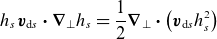 \begin{equation} h_{s}\boldsymbol{v}_{\text{d}s}\boldsymbol{\cdot }{\boldsymbol{\nabla }}_\perp h_{s} = \frac {1}{2}{\boldsymbol{\nabla }}_\perp \boldsymbol{\cdot } \left (\boldsymbol{v}_{\text{d}s} h_{s}^2\right ) \end{equation}
where the equality is correct to lowest order in (2.1) because $\boldsymbol{v}_{\text{d}s}$
is an equilibrium-like quantity whose perpendicular derivatives are small compared with those of
$\boldsymbol{v}_{\text{d}s}$
is an equilibrium-like quantity whose perpendicular derivatives are small compared with those of $h_{s}$
. Writing the velocity-space integral in terms of
$h_{s}$
. Writing the velocity-space integral in terms of $\varepsilon _{s}, \mu _{s}$
and
$\varepsilon _{s}, \mu _{s}$
and $\vartheta$
using
$\vartheta$
using
 \begin{equation} \int \textrm {d}^{3} \boldsymbol{v} = \sum _\sigma \int \frac {\textrm {d}\varepsilon _{s}\textrm {d}\mu _{s}\textrm {d}\vartheta }{m_{s}^2\left \rvert {v_\parallel }\right \rvert }B, \end{equation}
we find that the parallel streaming term in (B.7) also vanishes,
 \begin{align} &\left \langle \,\left \langle {\int \textrm {d}^{3} \boldsymbol{v} \left \langle \frac {T_{s}h_{s}}{F_{s}} v_\parallel {{\hat {\boldsymbol{b}}}}\boldsymbol{\cdot }{\boldsymbol{\nabla }}h_{s} \right \rangle _{\boldsymbol{r}}} \right \rangle _{\! \perp } \right \rangle _{\! \psi } \propto \left \langle \,\left \langle {\int \textrm {d}^{3} \boldsymbol{v}\, v_\parallel {{\hat {\boldsymbol{b}}}} \boldsymbol{\cdot } {\boldsymbol{\nabla }} \left (\frac {T_{s}}{F_{s}}\left \langle h_{s}^2 \right \rangle _{\boldsymbol{r}}\right )} \right \rangle _{\! \perp } \right \rangle _{\! \psi } \nonumber \\ &= \left \langle \,\left \langle {\sum _\sigma \int \frac {\textrm {d} \varepsilon _{s} \textrm {d} \mu _{s}\textrm {d}\vartheta }{m_{s}^2\left \rvert {v_\parallel }\right \rvert }v_\parallel \boldsymbol{B}\boldsymbol{\cdot }{\boldsymbol{\nabla }} \left (\frac {T_{s}}{F_{s}}\left \langle h_{s}^2 \right \rangle _{\boldsymbol{r}}\right )} \right \rangle _{\! \perp } \right \rangle _{\! \psi } \nonumber \\ &=\left \langle \,\left \langle {{\boldsymbol{\nabla }}\boldsymbol{\cdot }\sum _\sigma \int \sigma \frac {\textrm {d} \varepsilon _{s} \textrm {d} \mu _{s}\textrm {d}\vartheta }{m_{s}^2} \boldsymbol{B} \frac {T_{s}}{F_{s}}\left \langle h_{s}^2 \right \rangle _{\boldsymbol{r}}} \right \rangle _{\! \perp } \right \rangle _{\! \psi } = 0, \end{align}
where we used ${\boldsymbol{\nabla }} \boldsymbol{\cdot } \boldsymbol{B} = 0$
, (A.7), and the fact that
${\boldsymbol{\nabla }} \boldsymbol{\cdot } \boldsymbol{B} = 0$
, (A.7), and the fact that $T_{s}$
and
$T_{s}$
and $F_{s}$
vary only in the perpendicular direction to lowest order in (2.1).
$F_{s}$
vary only in the perpendicular direction to lowest order in (2.1).
To handle the first term in the square bracket in (B.7), we will need the following identity:
 \begin{align} &\left \langle \,\left \langle {\int \textrm {d}^{3} \boldsymbol{v} \left \langle h_{s} \left \langle \chi \right \rangle _{{\boldsymbol{R}_{s}}} \right \rangle _{\boldsymbol{r}}} \right \rangle _{\! \perp } \right \rangle _{\! \psi } \nonumber \\&= \left \langle \,\left \langle \sum _\sigma \! \int \! \frac {\textrm {d}\varepsilon _{s}\textrm {d}\mu _{s}\textrm {d}\vartheta }{m_{s}^2\left \rvert {v_\parallel }\right \rvert }B h_{s}\Big ({\boldsymbol{r}} - \boldsymbol{\rho }_{s}(\vartheta ), \varepsilon _{s}, \mu _{s}\Big )\right.\right. \quad \nonumber \\ &\qquad\ \left. \left. \int \! \frac {\textrm {d} \vartheta '}{2\pi }\chi \Big ({\boldsymbol{r}} - \boldsymbol{\rho }_{s}(\vartheta ) + \boldsymbol{\rho }_{s}(\vartheta '), \varepsilon _{s}, \mu _{s}, \vartheta '\Big )\! \right \rangle _{\! \perp } \right \rangle _{\! \psi } \nonumber \\&= \left \langle \,\left \langle {\sum _\sigma \! \int \! \frac {\textrm {d}\varepsilon _{s}\textrm {d}\mu _{s}\textrm {d}\vartheta }{m_{s}^2\left \rvert {v_\parallel }\right \rvert }B \int \frac {\textrm {d} \vartheta '}{2\pi } h_{s}\Big ({\boldsymbol{r}}' - \boldsymbol{\rho }_{s}(\vartheta '), \varepsilon _{s}, \mu _{s}\Big ) \chi ({\boldsymbol{r}}', \varepsilon _{s}, \mu _{s}, \vartheta ')} \right \rangle _{\! \perp } \right \rangle _{\! \psi } \nonumber \\&= \left \langle \,\left \langle {\sum _\sigma \! \int \! \frac {\textrm {d}\varepsilon _{s}\textrm {d}\mu _{s}\textrm {d}\vartheta '}{m_{s}^2\left \rvert {v_\parallel }\right \rvert }B h_{s}\Big ({\boldsymbol{r}}' - \boldsymbol{\rho }_{s}(\vartheta '), \varepsilon _{s}, \mu _{s}\Big ) \chi ({\boldsymbol{r}}', \varepsilon _{s}, \mu _{s}, \vartheta ')} \right \rangle _{\! \perp } \right \rangle _{\! \psi } \nonumber \\&= \left \langle \,\left \langle {\int \textrm {d}^{3} \boldsymbol{v} \left \langle h_{s} \chi \right \rangle _{\boldsymbol{r}}} \right \rangle _{\! \perp } \right \rangle _{\! \psi }, \end{align}
where, to obtain the final line, we have relabelled ${\boldsymbol{r}}' \mapsto {\boldsymbol{r}}$
,
${\boldsymbol{r}}' \mapsto {\boldsymbol{r}}$
, $\vartheta ' \mapsto \vartheta$
and used (B.9); the change of variables
$\vartheta ' \mapsto \vartheta$
and used (B.9); the change of variables ${\boldsymbol{r}}' = {\boldsymbol{r}} - \boldsymbol{\rho }_{s}(\vartheta ) + \boldsymbol{\rho }_{s}(\vartheta ')$
does not change the perpendicular spatial average in
${\boldsymbol{r}}' = {\boldsymbol{r}} - \boldsymbol{\rho }_{s}(\vartheta ) + \boldsymbol{\rho }_{s}(\vartheta ')$
does not change the perpendicular spatial average in $\langle \!\langle . \rangle _{\! \perp } \rangle _{\! \psi }$
to lowest order as
$\langle \!\langle . \rangle _{\! \perp } \rangle _{\! \psi }$
to lowest order as $\left \rvert {\boldsymbol{\rho }_{s}}\right \rvert \sim \rho _{s} \ll L$
. Using (B.11), we find
$\left \rvert {\boldsymbol{\rho }_{s}}\right \rvert \sim \rho _{s} \ll L$
. Using (B.11), we find
 \begin{align} &\sum _s q_{s} \left \langle \,\left \langle {\left \langle \int \textrm {d}^{3} \boldsymbol{v} h_{s}\frac {\partial {\left \langle \chi \right \rangle _{{\boldsymbol{R}_{s}}}}}{\partial {t}} \right \rangle _{\boldsymbol{r}}} \right \rangle _{\! \perp } \right \rangle _{\! \psi } &\nonumber \\ &= \left \langle \,\left \langle {\frac {\partial {\phi }}{\partial {t}} \sum _s q_{s} \int \textrm {d}^{3} \boldsymbol{v} \left \langle h_{s} \right \rangle _{\boldsymbol{r}}} \right \rangle _{\! \perp } \right \rangle _{\! \psi } - \left \langle \,\left \langle {\frac {\partial {\delta \boldsymbol{A}}}{\partial {t}} \boldsymbol{\cdot } \sum _s \frac {q_{s}}{c} \int \textrm {d}^{3} \boldsymbol{v} \left \langle {\boldsymbol{v}}h_{s} \right \rangle _{\boldsymbol{r}}} \right \rangle _{\! \perp } \right \rangle _{\! \psi } \nonumber \\ &= \frac {\textrm {d}^{}}{\textrm {d}{t}}\sum _s \left \langle \,\left \langle {\frac {q_{s}^2n_{s}}{2T_{s}}\phi ^2} \right \rangle _{\! \perp } \right \rangle _{\! \psi } - \left \langle \,\left \langle {\frac {\partial {\delta \boldsymbol{A}}}{\partial {t}}\boldsymbol{\cdot }\frac {{\boldsymbol{\nabla }}\times \delta \boldsymbol{B}}{4\pi }} \right \rangle _{\! \perp } \right \rangle _{\! \psi } \nonumber \\ &= \frac {\textrm {d}^{}}{\textrm {d}{t}}\sum _s \left \langle \,\left \langle {\frac {q_{s}^2n_{s}}{2T_{s}}\phi ^2} \right \rangle _{\! \perp } \right \rangle _{\! \psi } - \frac {\textrm {d}^{}}{\textrm {d}{t}}\left \langle \,\left \langle { \frac {\left \rvert {\delta \boldsymbol{B}}\right \rvert ^2}{8\pi }} \right \rangle _{\! \perp } \right \rangle _{\! \psi }, \end{align}
where we used (2.6) and (2.7). Therefore, adding together (B.4) and the second integral in (2.10) and taking a time derivative, we find
 \begin{equation} \frac {\textrm {d} {W}}{\textrm {d}{t}} = -\sum _s \left \langle \,\left \langle {\int \textrm {d}^{3} \boldsymbol{v} \left \langle \frac {T_{s}}{F_{s}}h_{s}\left \langle {\boldsymbol{v}_{\chi }} \right \rangle _{{\boldsymbol{R}_{s}}}\boldsymbol{\cdot }{\boldsymbol{\nabla }}F_{s} \right \rangle _{\boldsymbol{r}}} \right \rangle _{\! \perp } \right \rangle _{\! \psi }. \end{equation}
To calculate the right-hand side of (B.13), we use (2.14) to write, for a Maxwellian $F_{s}$
,
$F_{s}$
,
 \begin{align} {\boldsymbol{\nabla }} F_{s} = - {\boldsymbol{\nabla }} x \left [\frac {1}{L_{n_{s}}} + \frac {1}{L_{T_{s}}} \left ( \frac {v^2}{v_{\text{th}{s}}^2} - \frac {3}{2} \right ) \right ] F_{s}. \end{align}
Finally, using (B.11), we find that the time evolution of $W$
is given by (2.11)–(2.13).
$W$
is given by (2.11)–(2.13).
B.3 Expression for
$Y$

Let us now derive the expression (2.20) for the GK field invariant $Y$
. Expanding the first term in the integrand in (2.15), we find
$Y$
. Expanding the first term in the integrand in (2.15), we find
 \begin{equation} \sum _s \left \langle \,\left \langle {\int \textrm {d}^{3} \boldsymbol{v}\left \langle \frac {T_{s} h_{s}^2}{2F_{s}} - q_{s}\left \langle \chi \right \rangle _{{\boldsymbol{R}_{s}}}h_{s} + \frac {q_{s}^2\left (\left \langle \chi \right \rangle _{{\boldsymbol{R}_{s}}}\right )^2}{2T_{s}}F_{s} \right \rangle _{\boldsymbol{r}}} \right \rangle _{\! \perp } \right \rangle _{\! \psi }. \end{equation}
The second term in (B.15) is handled just like (B.12) to find
 \begin{align} &\sum _s \left \langle \,\left \langle {\int \textrm {d}^{3} \boldsymbol{v} \left \langle q_{s}\left \langle \chi \right \rangle _{{\boldsymbol{R}_{s}}}h_{s} \right \rangle _{\boldsymbol{r}}} \right \rangle _{\! \perp } \right \rangle _{\! \psi } = \left \langle \,\left \langle {\sum _s\frac {q_{s}^2n_{s}}{T_{s}}\phi ^2 - \frac {\left \rvert {{\boldsymbol{\nabla }}_\perp \delta A_\parallel }\right \rvert ^2}{4\pi } - \frac {\delta B_\parallel ^2}{4\pi }} \right \rangle _{\! \perp } \right \rangle _{\! \psi }. \end{align}
For the last term in the integrand in (B.15), we use the Fourier-space representation of the GK potential
 \begin{equation} \left \langle \chi \right \rangle _{{\boldsymbol{R}_{s}}} = \sum _{\boldsymbol{k}} \langle \chi \rangle _{{\boldsymbol{k}}_\perp } \textrm {e}^{\textrm {i} {\boldsymbol{k}}\boldsymbol{\cdot }{\boldsymbol{R}_{s}}}, \end{equation}
where
 \begin{align} \langle \chi \rangle _{{\boldsymbol{k}}_\perp } \equiv \textrm {J}_0(b_s)\left ({\phi }_{{\boldsymbol{k}}_\perp } - \frac {v_\parallel \delta {A}_{\parallel {{\boldsymbol{k}}_\perp }}}{c}\right ) + \frac {2\textrm {J}_1(b_s)}{b_s}\frac {T_{s}}{q_{s}}\frac {v_\perp ^2}{v_{\text{th}{s}}^2}\frac {\delta {B}_{\parallel {{\boldsymbol{k}}_\perp }}}{B}. \end{align}
Then,
 \begin{align} &\sum _s \left \langle \,\left \langle {\int \textrm {d}^{3} \boldsymbol{v} \left \langle \frac {q_{s}^2\left (\left \langle \chi \right \rangle _{{\boldsymbol{R}_{s}}}\right )^2}{2T_{s}}F_{s} \right \rangle _{\boldsymbol{r}}} \right \rangle _{\! \perp } \right \rangle _{\! \psi } \nonumber \\ &= \sum _{{{\boldsymbol{k}}_\perp }, s} \left \langle \int \textrm {d}^{3} \boldsymbol{v}\Bigg [ \frac {q_{s}^2}{2T_{s}}\left \rvert {{\phi }_{{\boldsymbol{k}}_\perp }}\right \rvert ^2\textrm {J}_0^2 + \frac {q_{s}^2v_\parallel ^2}{2c^2T_{s}}\left \rvert {\delta {A}_{\parallel {{\boldsymbol{k}}_\perp }}}\right \rvert ^2\textrm {J}_0^2 + \frac {T_{s}v_\perp ^4}{2v_{\text{th}{s}}^4}\left \rvert {\frac {\delta {B}_{\parallel {{\boldsymbol{k}}_\perp }}}{B}}\right \rvert ^2\frac {4\textrm {J}_1^2}{b_s^2} \Bigg .\right .\nonumber \\ &\left .\Bigg . \qquad \qquad \qquad + \frac {q_{s}v_\perp ^2}{2v_{\text{th}{s}}^2}\left ({\phi }_{{\boldsymbol{k}}_\perp }\frac {\delta {B}_{\parallel {{\boldsymbol{k}}_\perp }}^*}{B} +{\phi }_{{\boldsymbol{k}}_\perp }^*\frac {\delta {B}_{\parallel {{\boldsymbol{k}}_\perp }}}{B}\right ) \frac {2\textrm {J}_1\textrm {J}_0}{b_s} \Bigg ]F_{s}\right \rangle _\parallel . \end{align}
Using the identity
 \begin{equation} \int _0^{+\infty } \textrm {d} {x}\,x\textrm {J}_n(px)\textrm {J}_n(qx)\textrm {e}^{-ax^2} = \frac {1}{2a}\textrm {I}_n\left (\frac {pq}{2a}\right )\textrm {e}^{-(p^2+q^2)/2a}, \end{equation}
valid for any $n \in \mathbb{Z}$
, one can show that
$n \in \mathbb{Z}$
, one can show that
 \begin{align} &\int \textrm {d}^{3} \boldsymbol{v}\, \textrm {J}_0^2 F_{s} = n_{s} \mathrm{\Gamma }_{0s}, \end{align}
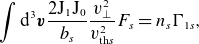 \begin{align} &\int \textrm {d}^{3} \boldsymbol{v} \frac {2\textrm {J}_1\textrm {J}_0}{b_s}\frac {v_\perp ^2}{v_{\text{th}{s}}^2}F_{s} = n_{s} \mathrm{\Gamma }_{1s}, \end{align}
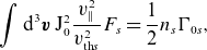 \begin{align} &\int \textrm {d}^{3} \boldsymbol{v}\, \textrm {J}_0^2\frac {v_\parallel ^2}{v_{\text{th}{s}}^2} F_{s} = \frac {1}{2}n_{s}\mathrm{\Gamma }_{0s}, \end{align}
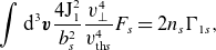 \begin{align} &\int \textrm {d}^{3} \boldsymbol{v} \frac {4\textrm {J}_1^2}{b_s^2}\frac {v_\perp ^4}{v_{\text{th}{s}}^4}F_{s} = 2n_{s}\mathrm{\Gamma }_{1s}, \\[6pt] \nonumber \end{align}
where $\mathrm{\Gamma }_{0s}$
and
$\mathrm{\Gamma }_{0s}$
and $\mathrm{\Gamma }_{1s}$
are defined in (2.21). Substituting (B.21)–(B.24) into (B.19), we find
$\mathrm{\Gamma }_{1s}$
are defined in (2.21). Substituting (B.21)–(B.24) into (B.19), we find
 \begin{align} &\sum _s \left \langle \,\left \langle {\int \textrm {d}^{3} \boldsymbol{v} \left \langle \frac {q_{s}^2\left (\left \langle \chi \right \rangle _{{\boldsymbol{R}_{s}}}\right )^2}{2T_{s}}F_{s} \right \rangle _{\boldsymbol{r}}} \right \rangle _{\! \perp } \right \rangle _{\! \psi } \nonumber \\ &=\sum _{{{\boldsymbol{k}}_\perp }, s}\left \langle \frac {q_{s}^2n_{s}\mathrm{\Gamma }_{0s}}{2T_{s}}\left \rvert {{\phi }_{{\boldsymbol{k}}_\perp }}\right \rvert ^2 + \frac {\mathrm{\Gamma }_{0s}\left \rvert {\delta {A}_{\parallel {{\boldsymbol{k}}_\perp }}}\right \rvert ^2}{8\pi d_{s}^2} + \frac {\beta _{s}\mathrm{\Gamma }_{1s}\left \rvert {\delta {B}_{\parallel {{\boldsymbol{k}}_\perp }}}\right \rvert ^2}{8\pi }\right . \nonumber \\ &\left .\qquad \qquad + \frac {q_{s}n_{s}\mathrm{\Gamma }_{1s}}{2}\left ({\phi }_{{\boldsymbol{k}}_\perp }\frac {\delta {B}_{\parallel {{\boldsymbol{k}}_\perp }}^*}{B} + {\phi }_{{\boldsymbol{k}}_\perp }^*\frac {\delta {B}_{\parallel {{\boldsymbol{k}}_\perp }}}{B}\right )\right \rangle _\parallel . \end{align}
Finally, combining (B.6), (B.15), (B.16) and (B.25), we arrive at (2.20). Note that combining the last two terms in (2.20) using
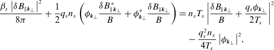 \begin{align} \frac {\beta _{s}\left \rvert {\delta {B}_{\parallel {{\boldsymbol{k}}_\perp }}}\right \rvert ^2}{8\pi } + \frac {1}{2}q_{s}n_{s}\left ({\phi }_{{\boldsymbol{k}}_\perp }\frac {\delta {B}_{\parallel {{\boldsymbol{k}}_\perp }}^*}{B} + {\phi }_{{\boldsymbol{k}}_\perp }^*\frac {\delta {B}_{\parallel {{\boldsymbol{k}}_\perp }}}{B}\right ) &= n_{s}T_{s}\left \rvert {\frac {\delta {B}_{\parallel {{\boldsymbol{k}}_\perp }}}{B} + \frac {q_{s}{\phi }_{{\boldsymbol{k}}_\perp }}{2T_{s}}}\right \rvert ^2\nonumber \\&\quad - \frac {q_{s}^2n_{s}}{4T_{s}}\left \rvert {{\phi }_{{\boldsymbol{k}}_\perp }}\right \rvert ^2\!, \end{align}
we can express $Y$
in terms of squares of the amplitudes as
$Y$
in terms of squares of the amplitudes as
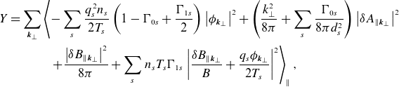 \begin{align} Y = \sum _{{\boldsymbol{k}}_\perp } &\left \langle -\sum _{s} \frac {q_{s}^2n_{s}}{2T_{s}}\left (1-\mathrm{\Gamma }_{0s} + \frac {\mathrm{\Gamma }_{1s}}{2}\right )\left \rvert {{\phi }_{{\boldsymbol{k}}_\perp }}\right \rvert ^2 + \left (\frac {k_\perp ^2}{8\pi } + \sum _s \frac {\mathrm{\Gamma }_{0s}}{8\pi d_{s}^2}\right )\left \rvert {\delta {A}_{\parallel {{\boldsymbol{k}}_\perp }}}\right \rvert ^2 \right .\nonumber \\ &\quad\!\!\left .+\frac {\left \rvert {\delta {B}_{\parallel {{\boldsymbol{k}}_\perp }}}\right \rvert ^2}{8\pi } + \sum _sn_{s}T_{s} \mathrm{\Gamma }_{1s} \left \rvert {\frac {\delta {B}_{\parallel {{\boldsymbol{k}}_\perp }}}{B} + \frac {q_{s}{\phi }_{{\boldsymbol{k}}_\perp }}{2T_{s}}}\right \rvert ^2\right \rangle _\parallel , \end{align}
where $\mathrm{\Gamma }_{0s}$
,
$\mathrm{\Gamma }_{0s}$
, $1 - \mathrm{\Gamma }_{0s}$
and
$1 - \mathrm{\Gamma }_{0s}$
and $\mathrm{\Gamma }_{1s}$
are all strictly positive.
$\mathrm{\Gamma }_{1s}$
are all strictly positive.
B.4 Injection terms for
$Y$

Taking a time derivative of the integral in (2.15) and substituting (2.4), we obtain
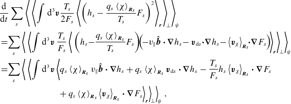 \begin{align} &\frac {\textrm {d}^{}}{\textrm {d}{t}}\sum _s \left \langle \,\left \langle {\int \textrm {d}^{3} \boldsymbol{v} \frac {T_{s}}{2F_{s}} \left \langle \left (h_{s} - \frac {q_{s}\left \langle \chi \right \rangle _{{\boldsymbol{R}_{s}}}}{T_{s}}F_{s}\right )^2 \right \rangle _{\boldsymbol{r}}} \right \rangle _{\! \perp } \right \rangle _{\! \psi } \nonumber \\ &=\!\sum _s\left \langle \,\left \langle {\int \textrm {d}^{3} \boldsymbol{v} \, \frac {T_{s}}{F_{s}} \left \langle \,\left (h_{s} \!-\! \frac {q_{s}\left \langle \chi \right \rangle _{{\boldsymbol{R}_{s}}}}{T_{s}}F_{s}\right ) \!\! \left (\!-v_\parallel {{\hat {\boldsymbol{b}}}}\boldsymbol{\cdot }{\boldsymbol{\nabla }}h_{s} \! - \boldsymbol{v}_{\text{d}s}\!\boldsymbol{\cdot }\!{\boldsymbol{\nabla }}h_{s}\!-\left \langle {\boldsymbol{v}_{\chi }} \right \rangle _{{\boldsymbol{R}_{s}}}\!\!\boldsymbol{\cdot }\!{\boldsymbol{\nabla }}F_{s}\right )\! \right \rangle _{\boldsymbol{r}}} \right \rangle _{\! \perp } \right \rangle _{\! \psi } \nonumber \\ &=\!\sum _s\left \langle \,\left \langle \int \textrm {d}^{3} \boldsymbol{v} \left \langle q_{s}\left \langle \chi \right \rangle _{{\boldsymbol{R}_{s}}}v_\parallel {{\hat {\boldsymbol{b}}}}\boldsymbol{\cdot }{\boldsymbol{\nabla }}h_{s} + q_{s} \left \langle \chi \right \rangle _{{\boldsymbol{R}_{s}}}\boldsymbol{v}_{\text{d}s}\boldsymbol{\cdot }{\boldsymbol{\nabla }}h_{s} - \frac {T_{s}}{F_{s}}h_{s}\left \langle {\boldsymbol{v}_{\chi }}\right \rangle _{{\boldsymbol{R}_{s}}}\boldsymbol{\cdot }{\boldsymbol{\nabla }}F_{s}\right .\right .\right . \nonumber \\ &\left .\left .\left . \qquad \qquad \qquad \ + \,q_{s} \left \langle \chi \right \rangle _{{\boldsymbol{R}_{s}}} \left \langle {\boldsymbol{v}_{\chi }} \right \rangle _{{\boldsymbol{R}_{s}}}\boldsymbol{\cdot }{\boldsymbol{\nabla }}F_{s}\right \rangle _{\boldsymbol{r}}\right \rangle _{\! \perp } \right \rangle _{\! \psi }, \end{align}
where the terms proportional to $h_{s} \boldsymbol{v}_{\text{d}s}\boldsymbol{\cdot }{\boldsymbol{\nabla }}h_{s}$
and
$h_{s} \boldsymbol{v}_{\text{d}s}\boldsymbol{\cdot }{\boldsymbol{\nabla }}h_{s}$
and $h_{s}v_\parallel {{\hat {\boldsymbol{b}}}}\boldsymbol{\cdot }{\boldsymbol{\nabla }}h_{s}$
have vanished for the same reason they did in (B.7). Additionally,
$h_{s}v_\parallel {{\hat {\boldsymbol{b}}}}\boldsymbol{\cdot }{\boldsymbol{\nabla }}h_{s}$
have vanished for the same reason they did in (B.7). Additionally,
 \begin{equation} \left \langle \chi \right \rangle _{{\boldsymbol{R}_{s}}} \left \langle {\boldsymbol{v}_{\chi }} \right \rangle _{{\boldsymbol{R}_{s}}}\boldsymbol{\cdot }{\boldsymbol{\nabla }}F_{s} = \left \langle \chi \right \rangle _{{\boldsymbol{R}_{s}}} \frac {c}{B} \left ({{\hat {\boldsymbol{b}}}} \times {\boldsymbol{\nabla }}_\perp \left \langle \chi \right \rangle _{{\boldsymbol{R}_{s}}}\right )\boldsymbol{\cdot } {\boldsymbol{\nabla }}F_{s} = -\frac {1}{2}{\boldsymbol{\nabla }}_\perp \boldsymbol{\cdot } \left (\left \langle \chi \right \rangle _{{\boldsymbol{R}_e}}^2 {{\hat {\boldsymbol{b}}}} \times {\boldsymbol{\nabla }}F_{s}\right ) \end{equation}
also vanishes to lowest order after integration [cf. (B.8)]. Finally, subtracting (B.13) from (B.28), we obtain (2.16).
Using (2.5) and (B.11), the magnetic-drift injection term becomes
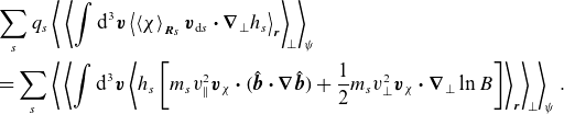 \begin{align} &\sum _s q_{s} \left \langle \,\left \langle {\int \textrm {d}^{3} \boldsymbol{v} \left \langle \left \langle \chi \right \rangle _{{\boldsymbol{R}_{s}}} \boldsymbol{v}_{\text{d}s}\boldsymbol{\cdot }{\boldsymbol{\nabla }}_\perp h_{s} \right \rangle _{\boldsymbol{r}}} \right \rangle _{\! \perp } \right \rangle _{\! \psi } \nonumber \\ &= \sum _s \left \langle \,\left \langle {\int \textrm {d}^{3} \boldsymbol{v} \left \langle h_{s} \left [m_{s}v_\parallel ^2 \boldsymbol{v}_{\chi }\boldsymbol{\cdot } ({{\hat {\boldsymbol{b}}}}\boldsymbol{\cdot }{\boldsymbol{\nabla }}{{\hat {\boldsymbol{b}}}}) + \frac {1}{2}m_{s}v_\perp ^2 \boldsymbol{v}_{\chi }\boldsymbol{\cdot } {\boldsymbol{\nabla }}_\perp \ln B \right ] \right \rangle _{\boldsymbol{r}}} \right \rangle _{\! \perp } \right \rangle _{\! \psi }. \end{align}
Using ${\boldsymbol{\nabla }}\times \boldsymbol{B} = (4\pi /c)\boldsymbol{J}$
and
${\boldsymbol{\nabla }}\times \boldsymbol{B} = (4\pi /c)\boldsymbol{J}$
and $\boldsymbol{J} \times \boldsymbol{B} = c{\boldsymbol{\nabla }} p$
, where
$\boldsymbol{J} \times \boldsymbol{B} = c{\boldsymbol{\nabla }} p$
, where $\boldsymbol{J}$
is the equilibrium current and
$\boldsymbol{J}$
is the equilibrium current and $p = \sum _s n_{s}T_{s}$
is the equilibrium pressure, (B.30) is simplified to (2.17).
$p = \sum _s n_{s}T_{s}$
is the equilibrium pressure, (B.30) is simplified to (2.17).
Appendix C. Derivation of the low-
$\beta$
drift-kinetic model

Our goal is to simplify the GK equation (2.4) in order to distil a minimum model for the good-curvature, electromagnetic instability discussed in § 3.2.2. First, we limit ourselves to the low- $\beta$
, zero-magnetic-shear
$\beta$
, zero-magnetic-shear $Z$
-pinch geometry, wherein (2.5) simplifies to
$Z$
-pinch geometry, wherein (2.5) simplifies to
 \begin{equation} \boldsymbol{v}_{\text{d}s} = -\frac {1}{\Omega _{s}{L_B}} \left ( v_\parallel ^2 + \frac {1}{2}v_\perp ^2 \right ){\hat {\boldsymbol{y}}}, \end{equation}
where
 \begin{equation} {L_B}^{-1} \equiv -{\hat {\boldsymbol{y}}} \boldsymbol{\cdot } ({{\hat {\boldsymbol{b}}}}\times {\boldsymbol{\nabla }} \ln B) \end{equation}
is the (inverse) length scale associated with the gradient of the magnetic-field strength. The main benefit of the $Z$
-pinch geometry is that (2.4) becomes homogeneous along the field lines. We are thus free to impose periodic boundary conditions in all three spatial dimensions and Fourier transform the distribution functionsFootnote
13
$Z$
-pinch geometry is that (2.4) becomes homogeneous along the field lines. We are thus free to impose periodic boundary conditions in all three spatial dimensions and Fourier transform the distribution functionsFootnote
13
 \begin{equation} h_{s} = \sum _{\boldsymbol{k}} {h}_{{s}{\boldsymbol{k}}} \textrm {e}^{\textrm {i} {\boldsymbol{k}}\boldsymbol{\cdot }{\boldsymbol{R}_{s}}} \end{equation}
and fields
 \begin{equation} \phi = \sum _{\boldsymbol{k}} {\phi }_{\boldsymbol{k}} \textrm {e}^{\textrm {i} {\boldsymbol{k}}\boldsymbol{\cdot }{\boldsymbol{r}}}, \quad \delta A_\parallel = \sum _{\boldsymbol{k}} \delta {A}_{\parallel {\boldsymbol{k}}} \textrm {e}^{\textrm {i} {\boldsymbol{k}}\boldsymbol{\cdot }{\boldsymbol{r}}}, \quad \delta B_\parallel = \sum _{\boldsymbol{k}} \delta {B}_{\parallel {\boldsymbol{k}}} \textrm {e}^{\textrm {i} {\boldsymbol{k}}\boldsymbol{\cdot }{\boldsymbol{r}}}. \end{equation}
Like in (B.18), the Fourier-transformed gyroaveraged GK potential is
 \begin{align} \left \langle \chi \right \rangle _{{\boldsymbol{R}_{s}}} = \sum _{\boldsymbol{k}} \langle \chi \rangle _{\boldsymbol{k}} \textrm {e}^{\textrm {i} {\boldsymbol{k}}\boldsymbol{\cdot }{\boldsymbol{R}_{s}}} = \sum _{\boldsymbol{k}} \left [\textrm {J}_0(b_s)\left ({\phi }_{\boldsymbol{k}} - \frac {v_\parallel \delta {A}_{\parallel {\boldsymbol{k}}}}{c}\right ) + \frac {2\textrm {J}_1(b_s)}{b_s}\frac {T_{s}}{q_{s}}\frac {v_\perp ^2}{v_{\text{th}{s}}^2}\frac {\delta {B}_{\parallel {\boldsymbol{k}}}}{B}\right ] \textrm {e}^{\textrm {i} {\boldsymbol{k}}\boldsymbol{\cdot }{\boldsymbol{R}_{s}}}. \end{align}
The GK equation (2.4) can then be written as
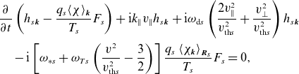 \begin{align} &\frac {\partial }{\partial t} \left ( {h}_{{s}{\boldsymbol{k}}} - \frac {q_{s} \langle \chi \rangle _{\boldsymbol{k}}}{T_{s}}F_{s} \right ) + \textrm {i} k_\parallel v_\parallel {h}_{{s}{\boldsymbol{k}}} + \textrm {i}\omega _{\text{d}s} \left (\frac {2v_\parallel ^2}{v_{\text{th}{s}}^2} + \frac {v_\perp ^2}{v_{\text{th}{s}}^2} \right ) {h}_{{s}{\boldsymbol{k}}} \nonumber \\ &\quad -\textrm {i} \left [ \omega _{*{s}} + \omega _{T{s}} \left ( \frac {v^2}{v_{\text{th}{s}}^2} - \frac {3}{2} \right ) \right ] \frac {q_{s} \left \langle \chi _{\boldsymbol{k}} \right \rangle _{{\boldsymbol{R}_{s}}}}{T_{s}}F_{s} = 0, \end{align}
where the drift frequencies are
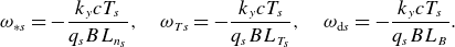 \begin{equation} \omega _{*{s}} = - \frac {k_y c T_{s}}{q_{s} B L_{n_{s}}}, \quad \omega _{T{s}} = -\frac {k_y c T_{s}}{q_{s} B L_{T_{s}}}, \quad \omega _{\text{d}s} = -\frac {k_y c T_{s}}{q_{s} B {L_B}}. \end{equation}
The field equations (2.7)–(2.9) become
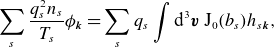 \begin{align} \sum _s \frac {q_{s}^2 n_{s}}{T_{s}} {\phi }_{\boldsymbol{k}} & = \sum _s q_{s} \int \textrm {d}^{3} \boldsymbol{v}\, \textrm {J}_0(b_s) {h}_{{s}{\boldsymbol{k}}}, \end{align}
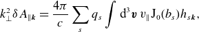 \begin{align} k_\perp ^2 \delta {A}_{\parallel {\boldsymbol{k}}} & = \frac {4\pi }{c} \sum _s q_{s} \int \textrm {d}^{3} \boldsymbol{v}\, v_\parallel \textrm {J}_0(b_s){h}_{{s}{\boldsymbol{k}}} , \end{align}
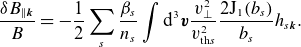 \begin{align} \frac {\delta {B}_{\parallel {\boldsymbol{k}}}}{B} &= - \frac {1}{2} \sum _s \frac {\beta _{s}}{n_{s}} \int \textrm {d}^{3} \boldsymbol{v} \frac {v_\perp ^2}{v_{\text{th}{s}}^2} \frac {2 \textrm {J}_1 (b_s)}{b_s} {h}_{{s}{\boldsymbol{k}}}. \\[6pt] \nonumber \end{align}
By restricting ourselves only to fluctuations that obey the orderings (3.1) and (3.2), we are able to make several simplifications. First, the contributions of $h_{i}$
to Maxwell’s equations (C.8)–(C.10) can be neglected because
$h_{i}$
to Maxwell’s equations (C.8)–(C.10) can be neglected because $\textrm {J}_0(b_i)\sim \textrm {J}_1(b_i)\sim (k_\perp \rho _{i})^{-1/2} \ll 1$
in the limit
$\textrm {J}_0(b_i)\sim \textrm {J}_1(b_i)\sim (k_\perp \rho _{i})^{-1/2} \ll 1$
in the limit $k_\perp \rho _{i} \gg 1$
, i.e. averaging over the large Larmor orbits of the ions results in an adiabatic ion response. Secondly,
$k_\perp \rho _{i} \gg 1$
, i.e. averaging over the large Larmor orbits of the ions results in an adiabatic ion response. Secondly, $k_\perp \rho _{e}\ll 1$
implies that the electrons become drift kinetic. This simplifies the Bessel functions in (C.5) and (C.8)–(C.10) to
$k_\perp \rho _{e}\ll 1$
implies that the electrons become drift kinetic. This simplifies the Bessel functions in (C.5) and (C.8)–(C.10) to $\textrm {J}_0(b_e) \approx 2\textrm {J}_1(b_e)/b_e \approx 1$
. Additionally,
$\textrm {J}_0(b_e) \approx 2\textrm {J}_1(b_e)/b_e \approx 1$
. Additionally, $\beta _{e} \ll 1$
implies that the parallel magnetic-field fluctuations are small. Indeed, using (C.9) and (C.10), we find
$\beta _{e} \ll 1$
implies that the parallel magnetic-field fluctuations are small. Indeed, using (C.9) and (C.10), we find
 \begin{equation} \frac {\delta B_\parallel }{\left \rvert {\delta \boldsymbol{B}_\perp }\right \rvert } \sim \frac {\delta {B}_{\parallel {\boldsymbol{k}}}}{k_\perp \delta {A}_{\parallel {\boldsymbol{k}}}} \sim \frac {m_{e}v_{\text{th}{e}}^2}{B} \frac {ck_\perp }{ev_{\text{th}{e}}} \sim k_\perp \rho _{e} \sim \sqrt {\beta _{e}} \ll 1. \end{equation}
Putting everything together, under the ordering (3.1), the low- $\beta$
dynamics are described by the electron drift-kinetic equation
$\beta$
dynamics are described by the electron drift-kinetic equation
 \begin{align} &\frac {\partial }{\partial t} \left ({h}_{{e}{\boldsymbol{k}}} + \frac {e{\phi }_{\boldsymbol{k}}}{T_{e}} F_{e} - \frac {2v_\parallel }{v_{\text{th}{e}}}\frac {\delta {A}_{\parallel {\boldsymbol{k}}}}{\rho _{e} B} F_{e} \right ) + \textrm {i}k_\parallel v_\parallel {h}_{{e}{\boldsymbol{k}}} + \textrm {i}\omega _{\text{d}e}\left (\frac {2v_\parallel ^2}{v_{\text{th}{e}}^2} + \frac {v_\perp ^2}{v_{\text{th}{e}}^2}\right ){h}_{{e}{\boldsymbol{k}}} \nonumber \\ &\quad + \textrm {i}\left [\omega _{*{e}} + \omega _{T{e}} \left ( \frac {v^2}{v_{\text{th}{s}}^2} - \frac {3}{2} \right ) \right ] \left (\frac {e{\phi }_{\boldsymbol{k}}}{T_{e}} - \frac {2v_\parallel }{v_{\text{th}{e}}}\frac {\delta {A}_{\parallel {\boldsymbol{k}}}}{\rho _{e} B}\right ) F_{e} = 0 \end{align}
and the field equations
 \begin{align} -(1 + \tau ^{-1})\frac {e{\phi }_{\boldsymbol{k}}}{T_{e}} &=\frac {1}{{n_{e}}}\int \textrm {d}^{3} \boldsymbol{v} {h}_{{e}{\boldsymbol{k}}} , \end{align}
 \begin{align} -k_\perp ^2d_{e}^2 \frac {\delta {A}_{\parallel {\boldsymbol{k}}}}{\rho _{e} B} &= \frac {1}{{n_{e}}}\int \textrm {d}^{3} \boldsymbol{v} \frac {v_\parallel }{v_{\text{th}{e}}}{h}_{{e}{\boldsymbol{k}}} = \frac {u_{\parallel {e}{\boldsymbol{k}}}}{v_{\text{th}{e}}}, \\[6pt] \nonumber \end{align}
where $u_{\parallel {e}}$
is the perturbed parallel electron flow. In the two-dimensional limit, viz.
$u_{\parallel {e}}$
is the perturbed parallel electron flow. In the two-dimensional limit, viz. $k_\parallel = 0$
, (C.12) decouples into its even part (in
$k_\parallel = 0$
, (C.12) decouples into its even part (in $v_\parallel$
)
$v_\parallel$
)
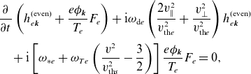 \begin{align} &\frac {\partial }{\partial t} \left ({h}_{{e}{\boldsymbol{k}}}^{\text{(even)}} + \frac {e{\phi }_{\boldsymbol{k}}}{T_{e}} F_{e}\right ) + \textrm {i} \omega _{\text{d}e}\left (\frac {2v_\parallel ^2}{v_{\text{th}{e}}^2} + \frac {v_\perp ^2}{v_{\text{th}{e}}^2}\right ){h}_{{e}{\boldsymbol{k}}}^{\text{(even)}} \nonumber \\ &\quad + \textrm {i}\left [\omega _{*{e}} + \omega _{T{e}} \left ( \frac {v^2}{v_{\text{th}{s}}^2} - \frac {3}{2} \right ) \right ] \frac {e{\phi }_{\boldsymbol{k}}}{T_{e}}F_{e} = 0, \end{align}
closed by (C.13), and its odd part
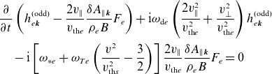 \begin{align} &\frac {\partial }{\partial t} \left ({h}_{{e}{\boldsymbol{k}}}^{\text{(odd)}} - \frac {2v_\parallel }{v_{\text{th}{e}}}\frac {\delta {A}_{\parallel {\boldsymbol{k}}}}{\rho _{e} B} F_{e} \right ) + \textrm {i} \omega _{\text{d}e}\left (\frac {2v_\parallel ^2}{v_{\text{th}{e}}^2} + \frac {v_\perp ^2}{v_{\text{th}{e}}^2}\right ){h}_{{e}{\boldsymbol{k}}}^{\text{(odd)}} \nonumber \\ &\quad - \textrm {i}\left [\omega _{*{e}} + \omega _{T{e}} \left ( \frac {v^2}{v_{\text{th}{s}}^2} - \frac {3}{2} \right ) \right ] \frac {2v_\parallel }{v_{\text{th}{e}}}\frac {\delta {A}_{\parallel {\boldsymbol{k}}}}{\rho _{e} B} F_{e} = 0 \end{align}
closed by (C.14).
C.1 Low-
$\beta$
conservation laws

Here, we use the orderings (3.1) and (3.2) to derive the asymptotic forms of the conservation laws (2.11) and (2.16).
First, the $h_{i}$
contribution to the free energy (B.1) is independently conserved and thus can be ignored. To see this, we use (2.4) to find
$h_{i}$
contribution to the free energy (B.1) is independently conserved and thus can be ignored. To see this, we use (2.4) to find
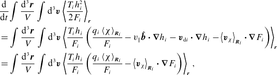 \begin{align} &\frac {\textrm {d}^{}}{\textrm {d}{t}} {\int \frac {\textrm {d}^{3} \boldsymbol{r}}{V}} \int \textrm {d}^{3} \boldsymbol{v} \left \langle \frac {T_{i}h_{i}^2}{2F_{i}} \right \rangle _{\boldsymbol{r}} \nonumber \\ &= {\int \frac {\textrm {d}^{3} \boldsymbol{r}}{V}} \int \textrm {d}^{3} \boldsymbol{v} \left \langle \frac {T_{i}h_{i}}{F_{i}}\left (\frac {q_{i} \left \langle \chi \right \rangle _{{\boldsymbol{R}_i}}}{F_{i}} - v_\parallel {{\hat {\boldsymbol{b}}}}\boldsymbol{\cdot }{\boldsymbol{\nabla }}h_{i} - \boldsymbol{v}_{\text{d}i} \boldsymbol{\cdot } {\boldsymbol{\nabla }} h_{i} - \left \langle {\boldsymbol{v}_{\chi }} \right \rangle _{{\boldsymbol{R}_{i}}}\boldsymbol{\cdot }{\boldsymbol{\nabla }}F_{i}\right ) \right \rangle _{\boldsymbol{r}} \nonumber \\ &= {\int \frac {\textrm {d}^{3} \boldsymbol{r}}{V}} \int \textrm {d}^{3} \boldsymbol{v} \left \langle \frac {T_{i}h_{i}}{F_{i}}\left (\frac {q_{i} \left \langle \chi \right \rangle _{{\boldsymbol{R}_i}}}{F_{i}} - \left \langle {\boldsymbol{v}_{\chi }}\right \rangle _{{\boldsymbol{R}_{i}}}\boldsymbol{\cdot }{\boldsymbol{\nabla }}F_{i}\right ) \right \rangle _{\boldsymbol{r}}, \end{align}
where the parallel-streaming and magnetic-drift terms vanish for the same reason as they do in the derivation of the free energy’s evolution equation given in Appendix B.2. For the remaining terms, we take advantage of the fact that, under (3.1), the ion gyroaverage of the GK potential is small, viz.
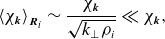 \begin{equation} \left \langle \chi _{\boldsymbol{k}} \right \rangle _{{\boldsymbol{R}_i}} \sim \frac {\chi _{\boldsymbol{k}}}{\sqrt {k_\perp \rho _{i}}} \ll \chi _{\boldsymbol{k}}, \end{equation}
where we used (B.18) and the asymptotic expansions
 \begin{equation} \left \rvert {\textrm {J}_0(x)}\right \rvert \sim \left \rvert {\textrm {J}_1(x)}\right \rvert \sim \frac {1}{\sqrt {x}}, \end{equation}
valid for $x \gg 1$
. Therefore, the last line of (C.17) vanishes to lowest order.
$x \gg 1$
. Therefore, the last line of (C.17) vanishes to lowest order.
Neglecting the $h_{i}$
contributions to (B.1), taking advantage of
$h_{i}$
contributions to (B.1), taking advantage of $k_\perp \rho _{e} \ll 1$
, dropping the parallel magnetic fluctuations, and using
$k_\perp \rho _{e} \ll 1$
, dropping the parallel magnetic fluctuations, and using
 \begin{align} \mathrm{\Gamma }_{0i} = O\left ({\frac {1}{k_\perp \rho _{i}}}\right ), \quad \mathrm{\Gamma }_{0e} = 1 - \frac {k_\perp ^2\rho _{e}^2}{2} + O\left ({k_\perp ^4\rho _{e}^4}\right ), \end{align}
 \begin{align} &\frac {\textrm {d} {W}}{\textrm {d}{t}} = \frac {Q^{\parallel }_e + Q^{\perp }_e}{L_{T_{e}}}, \quad \frac {\textrm {d}{Y}}{\textrm {d}{t}} = \left .\frac {\textrm {d}{Y}}{\textrm {d}{t}}\right \rvert _{\text{slab}} + \left .\frac {\textrm {d}{Y}}{\textrm {d}{t}}\right \rvert _{\text{drift}}, \end{align}
where
 \begin{align} &\left .\frac {\textrm {d}{Y}}{\textrm {d}{t}}\right \rvert _{\text{slab}} = {n_{e}}T_{e}v_{\text{th}{e}}{\int \frac {\textrm {d}^{3} \boldsymbol{r}}{V}}\! \left (\frac {u_{\parallel {e}}}{v_{\text{th}{e}}}\frac {\partial }{\partial {z}}\frac {e\phi }{T_{e}} + \frac {\delta A_\parallel }{\rho _{e} B}\:\frac {\partial }{\partial {z}}\frac {\delta p_{\parallel {e}}}{{n_{e}}T_{e}}\right ), \end{align}
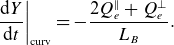 \begin{align} &\left .\frac {\textrm {d}{Y}}{\textrm {d}{t}}\right \rvert _{\text{curv}} = -\frac {2Q^{\parallel }_e + Q^{\perp }_e}{{L_B}}. \\[6pt] \nonumber \end{align}
The free energy and field invariant are given by
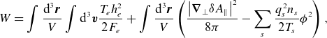 \begin{align} W &= {\int \frac {\textrm {d}^{3} \boldsymbol{r}}{V}}\int \textrm {d}^{3} \boldsymbol{v}\frac {T_{e}h_{e}^2}{2F_{e}} + {\int \frac {\textrm {d}^{3} \boldsymbol{r}}{V}}\left ( \frac {\left \rvert {{\boldsymbol{\nabla }}_\perp \delta A_\parallel }\right \rvert ^2}{8\pi } - \sum _s \frac {q_{s}^2n_{s}}{2T_{s}}\phi ^2\right ), \end{align}
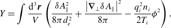 \begin{align} Y &= {\int \frac {\textrm {d}^{3} \boldsymbol{r}}{V}}\left (\frac {\delta A_\parallel ^2}{8\pi d_{e}^2} + \frac {\left \rvert {{\boldsymbol{\nabla }}_\perp \delta A_\parallel }\right \rvert ^2}{8\pi } -\frac {q_{i}^2{n_{i}}}{2T_{i}}\phi ^2\right ), \\[6pt] \nonumber \end{align}
respectively. In the above, $\delta p_{\parallel {e}} \equiv \int \textrm {d}^{3} \boldsymbol{v} m_{e}v_\parallel ^2h_{e}$
is the perturbed parallel electron pressure and
$\delta p_{\parallel {e}} \equiv \int \textrm {d}^{3} \boldsymbol{v} m_{e}v_\parallel ^2h_{e}$
is the perturbed parallel electron pressure and
 \begin{align} Q^{\parallel }_e &= \rho _{e}v_{\text{th}{e}}T_{e}{\int \frac {\textrm {d}^{3} \boldsymbol{r}}{V}} \int \textrm {d}^{3} \boldsymbol{v} \frac {v_\parallel ^2}{v_{\text{th}{e}}^2}\left (-\frac {1}{2}\frac {\partial }{\partial {y}}\frac {e\phi }{T_{e}} + \frac {v_\parallel }{v_{\text{th}{e}}}\frac {\partial }{\partial {y}}\frac {\delta A_\parallel }{\rho _{e} B}\right )h_{e}, \end{align}
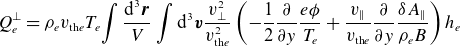 \begin{align} Q^{\perp }_e &= \rho _{e}v_{\text{th}{e}}T_{e}{\int \frac {\textrm {d}^{3} \boldsymbol{r}}{V}} \int \textrm {d}^{3} \boldsymbol{v} \frac {v_\perp ^2}{v_{\text{th}{e}}^2}\left (-\frac {1}{2}\frac {\partial }{\partial {y}}\frac {e\phi }{T_{e}} + \frac {v_\parallel }{v_{\text{th}{e}}}\frac {\partial }{\partial {y}}\frac {\delta A_\parallel }{\rho _{e} B}\right )h_{e} \\[6pt] \nonumber \end{align}
are the radial fluxes of energy associated with parallel and perpendicular electron motion, respectively. The first terms in the parentheses in (C.26) and (C.27) represent advection of parallel and perpendicular temperature, respectively, by the radial component of the $\boldsymbol{E}\times \boldsymbol{B}$
drift
$\boldsymbol{E}\times \boldsymbol{B}$
drift
 \begin{equation} \boldsymbol{v}_{E} \boldsymbol{\cdot } {\boldsymbol{\nabla }} x = -\frac {c}{B}\frac {\partial {\phi }}{\partial {y}}, \end{equation}
the second ones are the radial projection of transport along the exact field lines (sometimes called ‘flutter’ transport; Callen Reference Callen1977; Manheimer & Cook Reference Manheimer and Cook1978), whose radial perturbation is
 \begin{equation} \delta B_x = \frac {\partial {\delta A_\parallel }}{\partial {y}}. \end{equation}
Appendix D. Derivation of the low-
$\beta$
dispersion relation

The derivation of the dispersion relation is a direct application of the results of Ivanov & Adkins (Reference Ivanov and Adkins2023). The linear GK dispersion relation for a two-species, $Z$
-pinch plasma is
$Z$
-pinch plasma is
 \begin{equation} \left\lvert\begin{array}{l@{\quad}l@{\quad}l} L_{\phi \phi } & L_{\phi A} & L_{\phi B} \\ L_{A\phi } & L_{A A} & L_{A B} \\ L_{B\phi } & L_{B A} & L_{B B} \end{array}\right\rvert = 0, \end{equation}
where
 \begin{align} L_{\phi \phi } & = - \sum _s \frac {q_{s}^2 n_{s} T_{r}}{q_r^2 n_{r} T_{s}} \left \{ 1+ \left [\zeta _s - \zeta _{*s} + \eta _s \zeta _{*s} \left ( \partial _a + \partial _b + \frac {3}{2} \right ) \right ] \left .\mathcal{I}_{a,b}^{(s)} \right |_{a=b=1}\right \} , \end{align}
 \begin{align} L_{\phi A} & = 2\sum _s \frac {q_{s}^2 n_{s} v_{\text{th}{s}} T_{r}}{q_r^2 n_{r} v_{\text{th}{r}} T_{s}} \left [\zeta _s - \zeta _{*s} + \eta _s \zeta _{*s} \left ( \partial _a + \partial _b + \frac {3}{2} \right ) \right ] \left .\mathcal{J}_{a,b}^{(s)}\right |_{a=b=1}, \end{align}
 \begin{align} L_{\phi B} & = \sum _s \frac {q_{s} n_{s}}{q_r n_{r}} \left [\zeta _s - \zeta _{*s} + \eta _s \zeta _{*s} \left ( \partial _a + \partial _b + \frac {3}{2} \right ) \right ] \partial _b \left .{\mathcal{K}}_{a,b}^{(s)}\right |_{a=b=1}, \end{align}
 \begin{align} L_{A \phi } & = - \sum _s \frac {q_{s}^2 n_{s} v_{\text{th}{s}} T_{r}}{q_r^2 n_{r} v_{\text{th}{r}} T_{s}} \left [\zeta _s - \zeta _{*s} + \eta _s \zeta _{*s} \left ( \partial _a + \partial _b + \frac {3}{2} \right ) \right ] \left .\mathcal{J}_{a,b}^{(s)}\right |_{a=b=1} , \end{align}
 \begin{align} L_{AA} & = - \frac {B_0^2 ( k_\perp \rho _{r})^2}{8 \pi n_{r} T_{r}} - 2 \sum _s \frac {q_{s}^2 n_{s} m_r}{q_r^2 n_{r} m_s} \left [\zeta _s - \zeta _{*s} + \eta _s \zeta _{*s} \left ( \partial _a + \partial _b + \frac {3}{2} \right ) \right ] \partial _a \left .\mathcal{I}_{a,b}^{(s)}\right |_{a=b=1}, \end{align}
 \begin{align} L_{AB} & = \sum _s \frac {q_{s} n_{s} v_{\text{th}{s}}}{q_r n_{r} v_{\text{th}{r}}} \left [\zeta _s - \zeta _{*s} + \eta _s \zeta _{*s} \left ( \partial _a + \partial _b + \frac {3}{2} \right ) \right ] \partial _b \left .{\mathcal{L}}_{a,b}^{(s)}\right |_{a=b=1}, \\[8pt]\nonumber\end{align}
 \begin{align} L_{B\phi } & = - \sum _s \frac {\beta _s}{2} \frac {q_{s} T_{r}}{q_r T_{s}} \left [\zeta _s - \zeta _{*s} + \eta _s \zeta _{*s} \left ( \partial _a + \partial _b + \frac {3}{2} \right ) \right ] \partial _b \left .{\mathcal{K}}_{a,b}^{(s)}\right |_{a=b=1}, \end{align}
 \begin{align} L_{B A} & = \sum _s \beta _s \frac {q_{s} T_{r} v_{\text{th}{s}}}{q_r T_{s} v_{\text{th}{r}}} \left [\zeta _s - \zeta _{*s} + \eta _s \zeta _{*s} \left ( \partial _a + \partial _b + \frac {3}{2} \right ) \right ] \partial _b \left .{\mathcal{L}}_{a,b}^{(s)} \right |_{a=b=1}, \end{align}
 \begin{align} L_{BB} & = - 1 + \sum _s \frac {\beta _s}{2} \left [\zeta _s - \zeta _{*s} + \eta _s \zeta _{*s} \left ( \partial _a + \partial _b + \frac {3}{2} \right ) \right ] \partial _b^2 \left .{\mathcal{M}}_{a,b}^{(s)}\right |_{a=b=1}, \\[6pt] \nonumber \end{align}
where have normalised our expressions using an arbitrary reference species $r$
. We have also defined the following integrals:
$r$
. We have also defined the following integrals:
 \begin{align} \mathcal{I}_{a,b}^{(s)} & = \frac {1}{\sqrt {\pi }} \int _{-\infty }^\infty \textrm {d} u \int _0^\infty \textrm {d} \mu \: \frac { \textrm {e}^{-a u^2 - b \mu }}{u - \zeta _s + \left (2u^2 \zeta _{\kappa s} + \mu \zeta _{Bs} \right )} \textrm {J}_0^2(b_s), \end{align}
 \begin{align} \mathcal{J}_{a,b}^{(s)} & = \frac {1}{\sqrt {\pi }} \int _{-\infty }^\infty \textrm {d} u \int _0^\infty \textrm {d} \mu \: \frac { u \textrm {e}^{-a u^2 - b \mu }}{u - \zeta _s + \left (2u^2 \zeta _{\kappa s} + \mu \zeta _{Bs} \right )} \textrm {J}_0^2(b_s), \end{align}
 \begin{align} {\mathcal{K}}_{a,b}^{(s)} & = \frac {1}{\sqrt {\pi }} \int _{-\infty }^\infty \textrm {d} u \int _0^\infty \textrm {d} \mu \: \frac { \textrm {e}^{-a u^2 - b \mu }}{u - \zeta _s + \left (2u^2 \zeta _{\kappa s} + \mu \zeta _{Bs} \right )} \frac {2 \textrm {J}_0 (b_s) \textrm {J}_1 (b_s)}{b_s}, \end{align}
 \begin{align} {\mathcal{L}}_{a,b}^{(s)} & = \frac {1}{\sqrt {\pi }} \int _{-\infty }^\infty \textrm {d} u \int _0^\infty \textrm {d} \mu \: \frac { u \textrm {e}^{-a u^2 - b \mu }}{u - \zeta _s + \left (2u^2 \zeta _{\kappa s} + \mu \zeta _{Bs} \right )} \frac {2 \textrm {J}_0 (b_s) \textrm {J}_1 (b_s)}{b_s}, \end{align}
 \begin{align} {\mathcal{M}}_{a,b}^{(s)} & = \frac {1}{\sqrt {\pi }} \int _{-\infty }^\infty \textrm {d} u \int _0^\infty \textrm {d} \mu \: \frac { \textrm {e}^{-a u^2 - b \mu }}{u - \zeta _s + \left (2u^2 \zeta _{\kappa s} + \mu \zeta _{Bs} \right )} \left [\frac {2 \textrm {J}_1 (b_s)}{b_s} \right ]^2, \\[12pt] \nonumber \end{align}
and normalised frequencies
 \begin{align} \zeta _s = \frac {\textrm {i} p}{|k_\parallel | v_{\text{th}{s}}}, \quad \zeta _{*s} = \frac {\omega _{*s}}{|k_\parallel | v_{\text{th}{s}}}, \quad \zeta _{\kappa s} = \frac {\omega _{\kappa s}}{|k_\parallel | v_{\text{th}{s}}}, \quad \zeta _{{\boldsymbol{\nabla }} B s} = \frac {\omega _{{\boldsymbol{\nabla }} B s}}{|k_\parallel | v_{\text{th}{s}}}, \end{align}
where $\omega _{*{s}}$
is defined in (C.7) and the frequencies associated with the curvature and
$\omega _{*{s}}$
is defined in (C.7) and the frequencies associated with the curvature and ${\boldsymbol{\nabla }} B$
drifts are, respectively,
${\boldsymbol{\nabla }} B$
drifts are, respectively,
 \begin{align} \omega _{\kappa {s}} = \frac {v_{\text{th}{s}}^2 }{2\Omega _s} \boldsymbol{k}_\perp \boldsymbol{\cdot } \left [{{\hat {\boldsymbol{b}}}} \times ({{\hat {\boldsymbol{b}}}} \boldsymbol{\cdot } {\boldsymbol{\nabla }} ){{\hat {\boldsymbol{b}}}} \right ], \quad \omega _{{\boldsymbol{\nabla }} B{s}} = \frac {v_{\text{th}{s}}^2}{2\Omega _s} \boldsymbol{k}_\perp \boldsymbol{\cdot } \left ({{\hat {\boldsymbol{b}}}} \times {\boldsymbol{\nabla }} \ln B \right ). \end{align}
Using the orderings (3.1) and (3.2), we can make several simplifications to (D.2)–(D.10). First, $k_\perp \rho _{i} \gg 1$
implies that the ion integrals (D.11)–(D.15) are small since
$k_\perp \rho _{i} \gg 1$
implies that the ion integrals (D.11)–(D.15) are small since $b_i = k_\perp v_\perp /\Omega _{i} \sim k_\perp \rho _{i}$
and
$b_i = k_\perp v_\perp /\Omega _{i} \sim k_\perp \rho _{i}$
and $\textrm {J}_0(b_i) \to 0$
,
$\textrm {J}_0(b_i) \to 0$
, $\textrm {J}_1(b_i) \to 0$
as
$\textrm {J}_1(b_i) \to 0$
as $b_i \to \infty$
. Secondly, as the electrons are drift kinetic, viz.
$b_i \to \infty$
. Secondly, as the electrons are drift kinetic, viz. $b_e \sim k_\perp \rho _{e} \ll 1$
, we find that
$b_e \sim k_\perp \rho _{e} \ll 1$
, we find that $\textrm {J}_0(b_e) \to 1$
and
$\textrm {J}_0(b_e) \to 1$
and $2\textrm {J}_1(b_e)/b_e \to 1$
. Finally, the equilibrium pressure balance implies that, in the low-
$2\textrm {J}_1(b_e)/b_e \to 1$
. Finally, the equilibrium pressure balance implies that, in the low- $\beta$
limit,
$\beta$
limit, $\omega _{\kappa {s}} = \omega _{{\boldsymbol{\nabla }} B{s}} = \omega _{\text{d}s}$
, where the latter is defined in (C.7).
$\omega _{\kappa {s}} = \omega _{{\boldsymbol{\nabla }} B{s}} = \omega _{\text{d}s}$
, where the latter is defined in (C.7).
Combining all of this, the electron integrals (D.11)–(D.15) simplify as
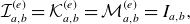 \begin{align} &\mathcal{I}_{a,b}^{(e)} = {\mathcal{K}}_{a,b}^{(e)} = {\mathcal{M}}_{a,b}^{(e)} = {I}_{a,b}, \end{align}
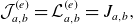 \begin{align} &\mathcal{J}_{a,b}^{(e)} = {\mathcal{L}}_{a,b}^{(e)} = {{J}_{a,b}}, \\[6pt] \nonumber \end{align}
where ${I}_{a,b}$
and
${I}_{a,b}$
and ${J}_{a,b}$
are given by
${J}_{a,b}$
are given by
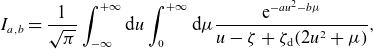 \begin{align} {I}_{a,b} &= \frac {1}{\sqrt {\pi }}\int _{-\infty }^{+\infty } \textrm {d} {u}\int _{0}^{+\infty } \textrm {d} {\mu } \frac {\textrm {e}^{-au^2 - b\mu }}{u - \zeta + \zeta _{\text{d}} (2u^2 + \mu )}, \end{align}
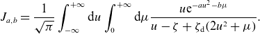 \begin{align} {{J}_{a,b}} &= \frac {1}{\sqrt {\pi }}\int _{-\infty }^{+\infty } \textrm {d} {u}\int _{0}^{+\infty } \textrm {d} {\mu } \frac {u\textrm {e}^{-au^2 - b\mu }}{u - \zeta + \zeta _{\text{d}} (2u^2 + \mu )}.\\[14pt] \nonumber\end{align}
We have normalised the frequencies as per (D.16) with $s = e$
, the normalised magnetic-drift frequency is
$s = e$
, the normalised magnetic-drift frequency is $\zeta _{\text{d}e} \equiv \omega _{\text{d}e} / \rvert k_\parallel \rvert v_{\text{th}{e}}$
, and the
$\zeta _{\text{d}e} \equiv \omega _{\text{d}e} / \rvert k_\parallel \rvert v_{\text{th}{e}}$
, and the $e$
subscript has been dropped. Finally, as
$e$
subscript has been dropped. Finally, as $\beta _{e} \ll 1$
, (D.8)–(D.10) imply
$\beta _{e} \ll 1$
, (D.8)–(D.10) imply $L_{B\phi } \to 0$
,
$L_{B\phi } \to 0$
, $L_{B A} \to 0$
and
$L_{B A} \to 0$
and $L_{B B} \to -1$
, so (D.1) becomes
$L_{B B} \to -1$
, so (D.1) becomes
 \begin{equation} 0 = \left\lvert\begin{array} {l@{\quad}l@{\quad}l}L_{\phi \phi } & L_{\phi A} & L_{\phi B} \\ L_{A\phi } & L_{A A} & L_{A B} \\ L_{B\phi } & L_{B A} & L_{B B} \end{array}\right\rvert = \left\lvert\begin{array} {c@{\quad}c@{\quad}c}L_{\phi \phi } & L_{\phi A} & L_{\phi B} \\ L_{A\phi } & L_{A A} & L_{A B} \\ 0 & 0 & -1 \end{array}\right\rvert = -(L_{\phi \phi } L_{A A} - L_{\phi A} L_{A\phi }), \end{equation}
where, using electrons as the reference species in (D.6)–(D.10) (i.e. setting $r=e$
), we have
$r=e$
), we have
 \begin{align} L_{\phi \phi } &= -1-\tau ^{-1} - \left [\zeta - \zeta _{*} + \zeta _{T} \left (\partial _a + \partial _b + \frac {3}{2}\right )\right ]\left .{I}_{a,b}\right \rvert _{a = b = 1}, \end{align}
 \begin{align} L_{A A} &= -k_\perp ^2d_{e}^2 - 2 \left [\zeta - \zeta _{*} + \zeta _{T} \left (\partial _a + \partial _b + \frac {3}{2}\right )\right ]\left .\partial _a {I}_{a,b}\right \rvert _{a = b = 1}, \end{align}
 \begin{align} L_{\phi A} &= -2L_{A\phi } = 2 \left [\zeta - \zeta _{*} + \zeta _{T} \left (\partial _a + \partial _b + \frac {3}{2}\right )\right ]\left .{{J}_{a,b}}\right \rvert _{a = b = 1}. \\[16pt] \nonumber \end{align}
Using the results of Ivanov & Adkins (Reference Ivanov and Adkins2023), we find
 \begin{align} &\!\!\left .{I}_{a,b}\right \rvert _{a = b = 1} = -\frac {1}{2\zeta _{\text{d}}}{\textrm {Z}_+}{\textrm {Z}_-}, \end{align}
 \begin{align} &\!\! \left .\partial _a{I}_{a,b}\right \rvert _{a = b = 1} = -\frac {1}{2\zeta _{\text{d}}}\left [2 + \frac {1}{\zeta _{\text{d}}}\left ({\textrm {Z}_+} - {\textrm {Z}_-}\right ) + \zeta _+{\textrm {Z}_-} + \zeta _-{\textrm {Z}_+} - \left (\frac {1}{4\zeta _{\text{d}}^2} - \frac {1}{2}{\textrm {Z}_+}{\textrm {Z}_-}\right )\right ], \end{align}
 \begin{align} &\!\!\left .{{J}_{a,b}}\right \rvert _{a = b = 1} = -\frac {1}{2\zeta _{\text{d}}}\left ({\textrm {Z}_+} - {\textrm {Z}_-} - \frac {{\textrm {Z}_+}{\textrm {Z}_-}}{2\zeta _{\text{d}}}\right ), \end{align}
 \begin{align} &\!\!\left (\!\partial _a + \partial _b + \frac {3}{2}\!\right )\left .{I}_{a,b}\right \rvert _{a = b = 1} = \frac {1}{2\zeta _{\text{d}}}\left [\zeta _+{\textrm {Z}_-} + \zeta _-{\textrm {Z}_+} + \left (\frac {\zeta }{\zeta _{\text{d}}} + \frac {1}{4\zeta _{\text{d}}^2} -1\right ){\textrm {Z}_+}{\textrm {Z}_-}\right ], \end{align}
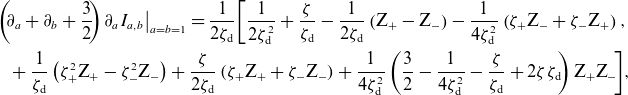 \begin{align} &\!\!\left (\!\partial _a + \partial _b + \frac {3}{2}\!\right )\!\left .\partial _a{I}_{a,b}\right \rvert _{a = b = 1} = \frac {1}{2\zeta _{\text{d}}}\bigg [\frac {1}{2\zeta _{\text{d}}^2} + \frac {\zeta }{\zeta _{\text{d}}} - \frac {1}{2\zeta _{\text{d}}}\left ({\textrm {Z}_+} - {\textrm {Z}_-}\right ) - \frac {1}{4\zeta _{\text{d}}^2}\left (\zeta _+{\textrm {Z}_-} + \zeta _-{\textrm {Z}_+}\right ),\nonumber \\&\!\!\!\quad + \frac {1}{\zeta _{\text{d}}}\left (\zeta _+^2{\textrm {Z}_+} - \zeta _-^2{\textrm {Z}_-}\right ) + \frac {\zeta }{2\zeta _{\text{d}}}\left (\zeta _+{\textrm {Z}_+} + \zeta _-{\textrm {Z}_-}\right ) + \frac {1}{4\zeta _{\text{d}}^2}\left (\frac {3}{2} - \frac {1}{4\zeta _{\text{d}}^2} - \frac {\zeta }{\zeta _{\text{d}}} + 2\zeta \zeta _{\text{d}}\!\right ){\textrm {Z}_+}{\textrm {Z}_-}\!\bigg ],\\[8pt]\nonumber \end{align}
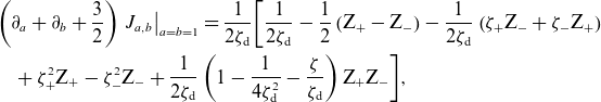 \begin{align} &\left (\partial _a + \partial _b + \frac {3}{2}\right )\left .{{J}_{a,b}}\right \rvert _{a = b = 1} = \frac {1}{2\zeta _{\text{d}}}\bigg [\frac {1}{2\zeta _{\text{d}}} - \frac {1}{2}\left ({\textrm {Z}_+} - {\textrm {Z}_-}\right ) - \frac {1}{2\zeta _{\text{d}}}\left (\zeta _+{\textrm {Z}_-} + \zeta _-{\textrm {Z}_+}\right ) \nonumber \\ &\quad + \zeta _+^2{\textrm {Z}_+} - \zeta _-^2{\textrm {Z}_-} + \frac {1}{2\zeta _{\text{d}}}\left (1 - \frac {1}{4\zeta _{\text{d}}^2}-\frac {\zeta }{\zeta _{\text{d}}}\right ){\textrm {Z}_+}{\textrm {Z}_-}\bigg ], \\[6pt] \nonumber \end{align}
where $\textrm {Z}_\pm = \textrm {Z}(\zeta _\pm )$
and
$\textrm {Z}_\pm = \textrm {Z}(\zeta _\pm )$
and
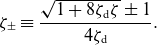 \begin{equation} \zeta _\pm \equiv \frac {\sqrt {1 + 8\zeta _{\text{d}}\zeta } \pm 1}{4\zeta _{\text{d}}}. \end{equation}
Substituting (D.26)–(D.31) into (D.23)–(D.25) and then into (D.22), we obtain a bulky but explicit dispersion relation for the system (C.12)–(C.14) that is straightforward to solve numerically.
D.1 Two-dimensional limit
The two-dimensional limit, i.e. $k_\parallel \to 0$
, corresponds to
$k_\parallel \to 0$
, corresponds to $\zeta \sim \zeta _{\text{d}} \to \infty$
, and so (D.32) becomes
$\zeta \sim \zeta _{\text{d}} \to \infty$
, and so (D.32) becomes
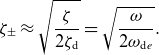 \begin{equation} \zeta _\pm \approx \sqrt {\frac {\zeta }{2\zeta _{\text{d}}}} = \sqrt {\frac {\omega }{2\omega _{\text{d}e}}}. \end{equation}
In writing (D.33), we have made use of our choice $\omega _{\text{d}e} \gt 0$
, which we discussed at the end of § 3. The two-dimensional limit is equivalent to dropping the
$\omega _{\text{d}e} \gt 0$
, which we discussed at the end of § 3. The two-dimensional limit is equivalent to dropping the $u$
term in the denominator of the integrands in (D.20) and (D.21). As its integrand becomes odd in
$u$
term in the denominator of the integrands in (D.20) and (D.21). As its integrand becomes odd in $u$
, (D.21) vanishes. In this case,
$u$
, (D.21) vanishes. In this case, $L_{\phi A} = L_{A\phi } = 0$
, so the dispersion relation (D.22) becomes
$L_{\phi A} = L_{A\phi } = 0$
, so the dispersion relation (D.22) becomes
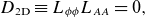 \begin{equation} D_{\text{2D}} \equiv L_{\phi \phi } L_{A A} = 0, \end{equation}
where $L_{\phi \phi }$
and
$L_{\phi \phi }$
and $L_{A A}$
are given by
$L_{A A}$
are given by
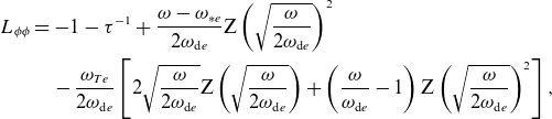 \begin{align} L_{\phi \phi } &= -1-\tau ^{-1}+\frac {\omega -\omega _{*{e}}}{2\omega _{\text{d}e}}\textrm {Z}\left (\sqrt {\frac {\omega }{2\omega _{\text{d}e}}}\right )^2 \nonumber \\ &\quad - \frac {\omega _{T{e}}}{2\omega _{\text{d}e}}\left [2\sqrt {\frac {\omega }{2\omega _{\text{d}e}}}\textrm {Z}\left (\sqrt {\frac {\omega }{2\omega _{\text{d}e}}}\right ) + \left (\frac {\omega }{\omega _{\text{d}e}}-1\right )\textrm {Z}\left (\sqrt {\frac {\omega }{2\omega _{\text{d}e}}}\right )^2\right ], \end{align}
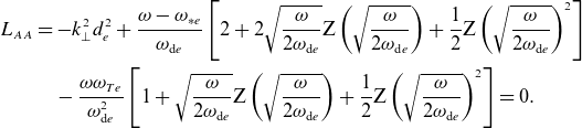 \begin{align} L_{A A}&=-k_\perp ^2d_{e}^2 + \frac {\omega - \omega _{*{e}}}{\omega _{\text{d}e}} \left [2 + 2\sqrt {\frac {\omega }{2\omega _{\text{d}e}}}\textrm {Z}\left (\sqrt {\frac {\omega }{2\omega _{\text{d}e}}}\right ) + \frac {1}{2}\textrm {Z}\left (\sqrt {\frac {\omega }{2\omega _{\text{d}e}}}\right )^2 \right ] \nonumber \\ &\quad -\frac {\omega \omega _{T{e}}}{\omega _{\text{d}e}^2}\left [1 + \sqrt {\frac {\omega }{2\omega _{\text{d}e}}}\textrm {Z}\left (\sqrt {\frac {\omega }{2\omega _{\text{d}e}}}\right ) +\frac {1}{2}\textrm {Z}\left (\sqrt {\frac {\omega }{2\omega _{\text{d}e}}}\right )^2 \right ]=0. \\[6pt] \nonumber \end{align}
Thus, the two-dimensional dispersion relation (D.34) splits into the electrostatic (3.4) and the electromagnetic (3.6) ones, given by $L_{\phi \phi } = 0$
and
$L_{\phi \phi } = 0$
and $L_{A A} = 0$
, respectively.
$L_{A A} = 0$
, respectively.
Appendix E. Fluid approximation for the MDM
To explore the cETG and MDM instabilities using a set of fluid moments, we follow Appendix A.5 of Adkins et al. (Reference Adkins, Schekochihin, Ivanov and Roach2022) and project the drift-kinetic equation (C.12) onto a set of Hermite (in $v_\parallel$
) and Laguerre (in
$v_\parallel$
) and Laguerre (in $v_\perp$
) basis functions. After truncating the infinite hierarchy to a total of
$v_\perp$
) basis functions. After truncating the infinite hierarchy to a total of $M$
Hermite and
$M$
Hermite and $L$
Laguerre functions, we obtain a set of
$L$
Laguerre functions, we obtain a set of $LM$
fluid equations, whose normal modes can be found by computing the eigenvalues of an
$LM$
fluid equations, whose normal modes can be found by computing the eigenvalues of an $LM\times LM$
matrix. The details of the decomposition can be found in Adkins et al. (Reference Adkins, Schekochihin, Ivanov and Roach2022). For the purposes of the discussion here,
$LM\times LM$
matrix. The details of the decomposition can be found in Adkins et al. (Reference Adkins, Schekochihin, Ivanov and Roach2022). For the purposes of the discussion here, $L$
and
$L$
and $M$
can be thought of as the ‘resolution’ of the fluid approximation in
$M$
can be thought of as the ‘resolution’ of the fluid approximation in $v_\perp$
and
$v_\perp$
and $v_\parallel$
, respectively.
$v_\parallel$
, respectively.
Panels (a) and (b) show the relative error between the unstable solution of (3.4) and that of the truncated Hermite–Laguerre hierarchy [see (A 64) of Adkins et al. (Reference Adkins, Schekochihin, Ivanov and Roach2022)] at varying numbers of Hermite and Laguerre moments, denoted by $M$
and
$M$
and $L$
, respectively, and two different values of
$L$
, respectively, and two different values of $\kappa _T$
, as labelled on the panels. We have set
$\kappa _T$
, as labelled on the panels. We have set $\kappa _n = 0$
. Here, we define the relative error between two quantities
$\kappa _n = 0$
. Here, we define the relative error between two quantities $a$
and
$a$
and $b$
as
$b$
as $\rvert {a-b}\rvert /\text{max}\lbrace \rvert {a}\rvert ,\rvert {b}\rvert \rbrace$
. Black denotes cases where the truncated fluid hierarchy has no unstable solution. For either
$\rvert {a-b}\rvert /\text{max}\lbrace \rvert {a}\rvert ,\rvert {b}\rvert \rbrace$
. Black denotes cases where the truncated fluid hierarchy has no unstable solution. For either $L = 0$
or
$L = 0$
or $M \lt 2$
, as
$M \lt 2$
, as $\kappa _T \to \infty$
, the growth rate is underpredicted by a factor of
$\kappa _T \to \infty$
, the growth rate is underpredicted by a factor of $\sqrt {2}$
and so the relative error converges to
$\sqrt {2}$
and so the relative error converges to $1 - 1/\sqrt {2} \approx 0.29$
. Panels (c) and (d) show the relative error for the MDM dispersion relation (3.6) at two different values of
$1 - 1/\sqrt {2} \approx 0.29$
. Panels (c) and (d) show the relative error for the MDM dispersion relation (3.6) at two different values of $\kappa _T$
and
$\kappa _T$
and $k_\perp ^2d_{e}^2$
, as labelled on each panel.
$k_\perp ^2d_{e}^2$
, as labelled on each panel.
Relative error between the unstable solutions obtained by solving the ETG (3.4) and the MDM (3.6) kinetic dispersion relations and those obtained from the truncated Hermite–Laguerre hierarchy at two different values of $(L, M)$
as a function of the temperature gradient
$(L, M)$
as a function of the temperature gradient $\kappa _T$
(as labelled in the legend). The ETG and MDM solutions are found at
$\kappa _T$
(as labelled in the legend). The ETG and MDM solutions are found at $\kappa _T \gt 0$
and
$\kappa _T \gt 0$
and $\kappa _T \lt 0$
, respectively. For both cases,
$\kappa _T \lt 0$
, respectively. For both cases, $\kappa _n = 0$
and
$\kappa _n = 0$
and $\tau = 1$
. To ensure that the MDM remains unstable as we increase
$\tau = 1$
. To ensure that the MDM remains unstable as we increase $\rvert{\kappa _T}\rvert$
, we have set
$\rvert{\kappa _T}\rvert$
, we have set $k_\perp ^2d_{e}^2 = -\kappa _T/5$
.
$k_\perp ^2d_{e}^2 = -\kappa _T/5$
.
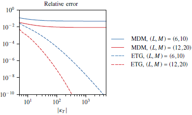
In figure 6(a,b), we show the relative error between the complex cETG frequency, obtained by solving (3.4) directly, and by finding the unstable normal mode of the truncated Hermite–Laguerre fluid hierarchy. As we increase the temperature gradient, the fluid and kinetic solutions converge as long as $M \gt 2$
and
$M \gt 2$
and $L \gt 1$
, i.e. if the fluctuations of parallel (3.11) and perpendicular (3.12) temperature are included in the fluid truncation. This is the expected behaviour given the discussion in § 3.2.1. If either
$L \gt 1$
, i.e. if the fluctuations of parallel (3.11) and perpendicular (3.12) temperature are included in the fluid truncation. This is the expected behaviour given the discussion in § 3.2.1. If either $\delta T_{\parallel {e}}$
or
$\delta T_{\parallel {e}}$
or $\delta T_{\perp {e}}$
is not included, it is easy to show that the resulting fluid dispersion relation is
$\delta T_{\perp {e}}$
is not included, it is easy to show that the resulting fluid dispersion relation is $\omega ^2 = -\omega _{T{e}}\omega _{\text{d}e}\tau$
, and thus the growth rate is underpredicted by a factor of
$\omega ^2 = -\omega _{T{e}}\omega _{\text{d}e}\tau$
, and thus the growth rate is underpredicted by a factor of $\sqrt {2}$
(see also Appendix G.1).
$\sqrt {2}$
(see also Appendix G.1).
The convergence of the kinetic and truncated-fluid solutions shows that the cETG instability is ‘fluidisable’, i.e. it can be described (asymptotically) using a set of fluid equations. The strongly driven limit $\kappa _T \to \infty$
is the natural one for the collisionless ‘fluidisation’ of the electron drift-kinetic equation (C.12). To see this, note that the frequencies in (C.12) can be split into two groups: the ‘kinetic frequencies’, containing the parallel streaming
$\kappa _T \to \infty$
is the natural one for the collisionless ‘fluidisation’ of the electron drift-kinetic equation (C.12). To see this, note that the frequencies in (C.12) can be split into two groups: the ‘kinetic frequencies’, containing the parallel streaming $k_\parallel v_\parallel$
and the magnetic drifts
$k_\parallel v_\parallel$
and the magnetic drifts $\omega _{\text{d}e}$
; and the ‘fluid frequencies’,
$\omega _{\text{d}e}$
; and the ‘fluid frequencies’, $\omega _{*{e}}$
and
$\omega _{*{e}}$
and $\omega _{T{e}}$
, which are proportional to the gradients of the plasma equilibrium profiles. In the Hermite–Laguerre decomposition, the terms proportional to the fluid frequencies appear only in the equations for the six lowest-order moments (Zocco & Schekochihin Reference Zocco and Schekochihin2011; Adkins et al. Reference Adkins, Schekochihin, Ivanov and Roach2022), while those proportional to the kinetic frequencies are responsible for coupling to higher-order moments.Footnote
14
Thus, in the strongly driven limit, wherein the fluid frequencies are asymptotically larger than the kinetic ones, if the mode frequency scales with the fluid frequencies [which is the case for the cETG dispersion relation (3.9)], the infinite hierarchy is asymptotically truncated to (at most) the six lowest-order moments. Note that this truncation is entirely collisionless.
$\omega _{T{e}}$
, which are proportional to the gradients of the plasma equilibrium profiles. In the Hermite–Laguerre decomposition, the terms proportional to the fluid frequencies appear only in the equations for the six lowest-order moments (Zocco & Schekochihin Reference Zocco and Schekochihin2011; Adkins et al. Reference Adkins, Schekochihin, Ivanov and Roach2022), while those proportional to the kinetic frequencies are responsible for coupling to higher-order moments.Footnote
14
Thus, in the strongly driven limit, wherein the fluid frequencies are asymptotically larger than the kinetic ones, if the mode frequency scales with the fluid frequencies [which is the case for the cETG dispersion relation (3.9)], the infinite hierarchy is asymptotically truncated to (at most) the six lowest-order moments. Note that this truncation is entirely collisionless.
In contrast to cETG, as discussed in § 3.2.2, the MDM satisfies $\omega \lesssim \omega _{\text{d}e}$
, and so we do not expect to be able to ‘fluidise’ it. In figure 6(c,d), we show the relative error between the MDM frequency, obtained by solving (3.6) directly, and by finding the unstable normal mode of the truncated Hermite–Laguerre fluid hierarchy. We observe that, even at very large values of the temperature gradient, the fluid approach does not provide a good approximation to the kinetic solution. To be more precise, for a fixed choice of
$\omega \lesssim \omega _{\text{d}e}$
, and so we do not expect to be able to ‘fluidise’ it. In figure 6(c,d), we show the relative error between the MDM frequency, obtained by solving (3.6) directly, and by finding the unstable normal mode of the truncated Hermite–Laguerre fluid hierarchy. We observe that, even at very large values of the temperature gradient, the fluid approach does not provide a good approximation to the kinetic solution. To be more precise, for a fixed choice of $L$
and
$L$
and $M$
, it is impossible to find parameters
$M$
, it is impossible to find parameters $\kappa _T$
and
$\kappa _T$
and $k_\perp ^2d_{e}^2$
for which the kinetic and fluid solutions converge to each other. This is further illustrated in figure 7 where we vary
$k_\perp ^2d_{e}^2$
for which the kinetic and fluid solutions converge to each other. This is further illustrated in figure 7 where we vary $\kappa _T$
for fixed
$\kappa _T$
for fixed $L$
and
$L$
and $M$
. We find that as
$M$
. We find that as $\kappa _T \to \infty$
, the error in the ETG solution decreases to zero. In contrast, as
$\kappa _T \to \infty$
, the error in the ETG solution decreases to zero. In contrast, as $\kappa _T \to -\infty$
, the error in the MDM solution converges to a finite, non-zero value. Thus, we conclude that the MDM cannot be captured by a finite set of fluid equations.Footnote
15
$\kappa _T \to -\infty$
, the error in the MDM solution converges to a finite, non-zero value. Thus, we conclude that the MDM cannot be captured by a finite set of fluid equations.Footnote
15
Appendix F. The MDM stability boundaries
Since the complex solutions $\omega$
to (3.6) are a smooth function of the parameters
$\omega$
to (3.6) are a smooth function of the parameters $k_\perp ^2d_{e}^2$
,
$k_\perp ^2d_{e}^2$
, ${L_B}/L_{T_{e}}$
and
${L_B}/L_{T_{e}}$
and ${L_B}/L_{n_{e}}$
, the region of instability seen in figure 3 is bounded by lines on which
${L_B}/L_{n_{e}}$
, the region of instability seen in figure 3 is bounded by lines on which $\omega \in \mathbb{R}$
, the stability boundaries. Recall that we have assumed that
$\omega \in \mathbb{R}$
, the stability boundaries. Recall that we have assumed that $\omega _{\text{d}e} \gt 0$
. Therefore,
$\omega _{\text{d}e} \gt 0$
. Therefore, $\sqrt {\omega /2\omega _{\text{d}e}}$
, which appears as the argument of the
$\sqrt {\omega /2\omega _{\text{d}e}}$
, which appears as the argument of the $\textrm {Z}$
functions in (3.6), lies on the positive real or positive imaginary axes if
$\textrm {Z}$
functions in (3.6), lies on the positive real or positive imaginary axes if $\omega \gt 0$
or
$\omega \gt 0$
or $\omega \lt 0$
, respectively. When
$\omega \lt 0$
, respectively. When $\omega \gt 0$
, we recover the upper solid black line in figure 3, while the lower one corresponds to
$\omega \gt 0$
, we recover the upper solid black line in figure 3, while the lower one corresponds to $\omega \lt 0$
. The dashed black line in figure 3 is a special case of the stability boundary where
$\omega \lt 0$
. The dashed black line in figure 3 is a special case of the stability boundary where $\omega = 0$
, not just its imaginary part. Let us try to understand this feature of figure 3 first.
$\omega = 0$
, not just its imaginary part. Let us try to understand this feature of figure 3 first.
F.1 Small-
$\omega$
limit

In the limit $\omega /\omega _{\text{d}e} \sim \delta \ll 1$
, we can expand the
$\omega /\omega _{\text{d}e} \sim \delta \ll 1$
, we can expand the $\textrm {Z}$
functions in the dispersion relation using
$\textrm {Z}$
functions in the dispersion relation using
 \begin{equation} \textrm {Z}(\zeta ) = \textrm {i}\sqrt {\pi } - 2\zeta -\textrm {i}\zeta ^2 + \frac {4}{3}\zeta ^3 + O\left ({\zeta ^4}\right ), \end{equation}
to obtain from (D.36)
 \begin{align} L_{A A} = &-k_\perp ^2d_{e}^2 - \frac {4-\pi }{2}\kappa _n + \frac {4-\pi - (\pi -2)(\kappa _n-\kappa _T)}{2}\frac {\omega }{\omega _{\text{d}e}} \nonumber \\ &- \textrm {i} \sqrt {\frac {\pi }{2}}\frac {2\kappa _n-3\kappa _T}{3}\left (\frac {\omega }{\omega _{\text{d}e}}\right )^{3/2} + O\left ({\delta ^2}\right ). \end{align}
Keeping only terms to $O({\delta ^0})$
, we find that
$O({\delta ^0})$
, we find that $\omega \ll \omega _{\text{d}e}$
solutions to
$\omega \ll \omega _{\text{d}e}$
solutions to $L_{A A} = 0$
exist only if
$L_{A A} = 0$
exist only if $k_\perp ^2d_{e}^2 + (4-\pi )\kappa _n/2 \sim \delta \ll 1$
. Indeed, the horizontal dotted line in figure 3, which specifies the minimum
$k_\perp ^2d_{e}^2 + (4-\pi )\kappa _n/2 \sim \delta \ll 1$
. Indeed, the horizontal dotted line in figure 3, which specifies the minimum $k_\perp ^2d_{e}^2$
for the instability and on which
$k_\perp ^2d_{e}^2$
for the instability and on which $\omega = 0$
is an exact solution, is
$\omega = 0$
is an exact solution, is $k_\perp ^2d_{e}^2 = k_{\perp \text{,min}}^2d_{e}^2$
, where
$k_\perp ^2d_{e}^2 = k_{\perp \text{,min}}^2d_{e}^2$
, where
 \begin{equation} k_{\perp \text{,min}}^2d_{e}^2 = -\frac {4-\pi }{2}\kappa _n. \end{equation}
Note that (3.13) implies that $\omega = 0$
is a solution only if
$\omega = 0$
is a solution only if $\kappa _n \lt 0$
. Expanding
$\kappa _n \lt 0$
. Expanding
 \begin{equation} \omega = \omega _0 + \omega _1 + \dots \end{equation}
in $\delta \ll 1$
, we find
$\delta \ll 1$
, we find
 \begin{equation} \frac {\omega _0}{\omega _{\text{d}e}} = \frac {2k_\perp ^2d_{e}^2 + (4-\pi )\kappa _T}{4-\pi - (\pi -2)(\kappa _n - \kappa _T)}. \end{equation}
Thus, to lowest order, $\omega \approx \omega _0 \in \mathbb{R}$
.
$\omega \approx \omega _0 \in \mathbb{R}$
.
To determine the growth rate, we proceed to next order, which, in combination with (F.5), yields
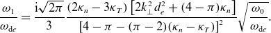 \begin{align} \frac {\omega _1}{\omega _{\text{d}e}} &= \frac {\textrm {i}\sqrt {2\pi }}{3}\frac {(2\kappa _n-3\kappa _T)\left [2k_\perp ^2d_{e}^2 + (4-\pi )\kappa _n\right ]}{\left [4-\pi -(\pi -2)(\kappa _n-\kappa _T)\right ]^2}\sqrt {\frac {\omega _0}{\omega _{\text{d}e}}}. \end{align}
If $\omega _0/\omega _{\text{d}e} \lt 0$
, then
$\omega _0/\omega _{\text{d}e} \lt 0$
, then $\omega _1$
is again purely real. In fact, it is not difficult to see that if
$\omega _1$
is again purely real. In fact, it is not difficult to see that if $\omega _0/\omega _{\text{d}e} \lt 0$
, then all terms in the perturbative expansion (F.4) are purely real. This happens because all integer powers of
$\omega _0/\omega _{\text{d}e} \lt 0$
, then all terms in the perturbative expansion (F.4) are purely real. This happens because all integer powers of $\omega$
in the expansion (F.2) have real coefficients while the half-integer ones have purely imaginary ones, which is itself a consequence of the pattern of alternating purely imaginary and purely real coefficients in the expansion of the
$\omega$
in the expansion (F.2) have real coefficients while the half-integer ones have purely imaginary ones, which is itself a consequence of the pattern of alternating purely imaginary and purely real coefficients in the expansion of the $\textrm {Z}$
function (F.1). Therefore, the small-
$\textrm {Z}$
function (F.1). Therefore, the small- $\omega$
expansion can yield solutions with finite
$\omega$
expansion can yield solutions with finite $\text{Im}\:\omega$
only if
$\text{Im}\:\omega$
only if $\omega _0/\omega _{\text{d}e} \gt 0$
.
$\omega _0/\omega _{\text{d}e} \gt 0$
.
If this is satisfied, then (F.6) has a positive imaginary part if
 \begin{equation} (2\kappa _n-3\kappa _T)\left [2k_\perp ^2d_{e}^2 + (4-\pi )\kappa _n\right ] \gt 0. \end{equation}
Suppose that
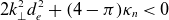 \begin{equation} 2k_\perp ^2d_{e}^2 + (4-\pi )\kappa _n \lt 0 \end{equation}
and
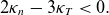 \begin{equation} 2\kappa _n-3\kappa _T \lt 0. \end{equation}
Since we have demanded $\omega _0/\omega _{\text{d}e} \gt 0$
, we need, from (F.5),
$\omega _0/\omega _{\text{d}e} \gt 0$
, we need, from (F.5),
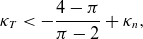 \begin{equation} \kappa _T \lt -\frac {4-\pi }{\pi -2} + \kappa _n, \end{equation}
which, together with (F.9), yields
 \begin{equation} \frac {\kappa _n}{3} \gt \frac {4-\pi }{\pi -2}, \end{equation}
which is a contradiction with the assumption (F.8), which is impossible when $\kappa _n \lt 0$
. Thus, (F.7) can be fulfilled only if
$\kappa _n \lt 0$
. Thus, (F.7) can be fulfilled only if
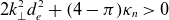 \begin{equation} 2k_\perp ^2d_{e}^2 + (4-\pi )\kappa _n \gt 0 \end{equation}
and
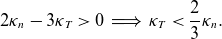 \begin{equation} 2\kappa _n-3\kappa _T \gt 0 \implies \kappa _T \lt \frac {2}{3}\kappa _n. \end{equation}
Combining (F.12) and (F.5), we find also that
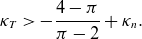 \begin{equation} \kappa _T \gt -\frac {4-\pi }{\pi -2} + \kappa _n. \end{equation}
Together, (F.13) and (F.14) give the left- and right-hand ends of the horizontal dashed line in figure 3, respectively.
F.2 Finite positive
$\omega$

Now, we turn to the case of marginal stability with the real frequency $\omega \gt 0$
and let
$\omega \gt 0$
and let $s \equiv \sqrt {\omega /2\omega _{\text{d}e}}$
, so the
$s \equiv \sqrt {\omega /2\omega _{\text{d}e}}$
, so the $\textrm {Z}$
functions in (3.6) become
$\textrm {Z}$
functions in (3.6) become
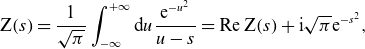 \begin{equation} \textrm {Z}(s) = \frac {1}{\sqrt {\pi }} \int _{-\infty }^{+\infty } \textrm {d} {u} \frac {\textrm {e}^{-u^2}}{u-s} = \text{Re}\:\textrm {Z}(s) + \textrm {i} \sqrt {\pi }\textrm {e}^{-s^2}, \end{equation}
where, since $s \in \mathbb{R}^+$
, the real part of
$s \in \mathbb{R}^+$
, the real part of $\textrm {Z}$
is given by the principal value of (3.5), viz.
$\textrm {Z}$
is given by the principal value of (3.5), viz.
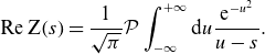 \begin{equation} \text{Re}\:\textrm {Z}(s) = \frac {1}{\sqrt {\pi }} \mathcal{P}\int _{-\infty }^{+\infty } \textrm {d} {u} \frac {\textrm {e}^{-u^2}}{u-s}. \end{equation}
Taking the imaginary part of the dispersion relation (3.6), we find
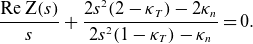 \begin{equation} \frac {\text{Re}\:\textrm {Z}(s)}{s} + \frac {2s^2(2 - \kappa _T) - 2\kappa _n}{2s^2(1 - \kappa _T) - \kappa _n}=0. \end{equation}
We now take two limits of (F.17): $s \ll 1$
and
$s \ll 1$
and $\kappa _T \gg 1$
.
$\kappa _T \gg 1$
.
When $s \ll 1$
, we can use (F.1), to expand
$s \ll 1$
, we can use (F.1), to expand
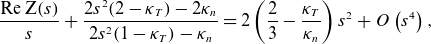 \begin{align} &\frac {\text{Re}\:\textrm {Z}(s)}{s} + \frac {2s^2(2 - \kappa _T) - 2\kappa _n}{2s^2(1 - \kappa _T) - \kappa _n} = 2\left (\frac {2}{3} - \frac {\kappa _T}{\kappa _n}\right )s^2 + O\left ({s^4}\right ), \end{align}
which then implies that the solution of (F.17) satisfies $s \to 0$
only if
$s \to 0$
only if $\kappa _T \to 2\kappa _n/3$
. This connects the positive-
$\kappa _T \to 2\kappa _n/3$
. This connects the positive- $\omega$
stability boundary to the left end of the small-
$\omega$
stability boundary to the left end of the small- $\omega$
stability boundary given by (F.13).
$\omega$
stability boundary given by (F.13).
In the strongly driven limit $\kappa _T \gg 1$
, (F.17) gives
$\kappa _T \gg 1$
, (F.17) gives $\text{Re}\:\textrm {Z}(s)\approx -s$
, which has a unique solution at
$\text{Re}\:\textrm {Z}(s)\approx -s$
, which has a unique solution at $s \approx 1.063$
. In this limit, the dispersion relation (3.6) becomes
$s \approx 1.063$
. In this limit, the dispersion relation (3.6) becomes
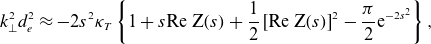 \begin{equation} k_\perp ^2d_{e}^2 \approx -2s^2\kappa _T\left \lbrace 1+s\text{Re}\:\textrm {Z}(s) + \frac {1}{2}\left [\text{Re}\:\textrm {Z}(s)\right ]^2-\frac {\pi }{2}\textrm {e}^{-2s^2}\right \rbrace , \end{equation}
which, upon substitution of $s \approx 1.063$
, gives us
$s \approx 1.063$
, gives us
 \begin{equation} k_\perp ^2d_{e}^2 \approx -0.61\kappa _T. \end{equation}
This is the asymptotic slope of the top solid line in figure 3.
F.3 Finite negative
$\omega$

If $\omega \lt 0$
, then the argument of the
$\omega \lt 0$
, then the argument of the $\textrm {Z}$
functions in (3.6) is purely imaginary. Let
$\textrm {Z}$
functions in (3.6) is purely imaginary. Let
 \begin{equation} \sqrt {\frac {\omega }{2\omega _{\text{d}e}}} \equiv \textrm {i} v, \end{equation}
where $v \gt 0$
. Then, (3.5) implies
$v \gt 0$
. Then, (3.5) implies $\textrm {Z}(\textrm {i} v) = \textrm {i} \text{Im} \: \textrm {Z}(\textrm {i} v)$
, where
$\textrm {Z}(\textrm {i} v) = \textrm {i} \text{Im} \: \textrm {Z}(\textrm {i} v)$
, where
 \begin{equation} \text{Im} \:\textrm {Z}(\textrm {i} v) = \frac {v}{\sqrt {\pi }}\int _{-\infty }^{+\infty } \textrm {d} {u} \frac {\textrm {e}^{-u^2}}{u^2 + v^2}. \end{equation}
In this case, the dispersion relation (3.6) is purely real and can be written as
 \begin{equation} k_\perp ^2d_{e}^2 = -\left (2v^2 + \kappa _n\right ) \left [2 - 2v\:\text{Im}\:\textrm {Z} - \frac {1}{2}\left (\text{Im}\:\textrm {Z}\right )^2\right ] + 2v^2\kappa _T \left [1 - v\:\text{Im}\:\textrm {Z} - \frac {1}{2}\left (\text{Im}\:\textrm {Z}\right )^2\right ]. \end{equation}
Once again, we consider two limits: $v \ll 1$
and
$v \ll 1$
and $\kappa _T \gg 1$
.
$\kappa _T \gg 1$
.
When $v \ll 1$
, we expand (F.23) to find
$v \ll 1$
, we expand (F.23) to find
 \begin{align} k_\perp ^2d_{e}^2 = &-\frac {4-\pi }{2}\kappa _n - \left [4-\pi -(\pi -2)\left (\kappa _n-\kappa _T\right )\right ]v^2 \nonumber \\ &+ 2\sqrt {\pi }\left (\kappa _T-\frac {2}{3}\kappa _n\right )v^3 + O\left ({v^4}\right ). \end{align}
Anticipating that the negative- $\omega$
stability boundary connects to the right-hand end (F.14) of the small-
$\omega$
stability boundary connects to the right-hand end (F.14) of the small- $\omega$
one, (F.13) and (F.14) imply that the coefficients of
$\omega$
one, (F.13) and (F.14) imply that the coefficients of $v^2$
and
$v^2$
and $v^3$
in (F.24) are positive and negative, respectively. Thus, the right-hand side of (F.24) peaks at finite
$v^3$
in (F.24) are positive and negative, respectively. Thus, the right-hand side of (F.24) peaks at finite $v \gt 0$
, and so (F.24) can be solved for any
$v \gt 0$
, and so (F.24) can be solved for any $k_\perp ^2d_{e}^2$
up to the value of that peak. Differentiating the right-hand side of (F.24) and substituting the value of
$k_\perp ^2d_{e}^2$
up to the value of that peak. Differentiating the right-hand side of (F.24) and substituting the value of $v$
at the local maximum, we find
$v$
at the local maximum, we find
 \begin{equation} k_\perp ^2d_{e}^2 = -\frac {4-\pi }{2}\kappa _n - \frac {\left [4-\pi -(\pi -2)\left (\kappa _n-\kappa _T\right )\right ]^3}{3\pi \left (3\kappa _T-2\kappa _n\right )^2}. \end{equation}
Thus, the start of the bottom solid line in figure 3 is a cubic curve.
In the strongly driven limit $\kappa _T \gg 1$
, (F.23) simplifies to
$\kappa _T \gg 1$
, (F.23) simplifies to
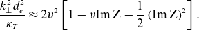 \begin{equation} \frac {k_\perp ^2d_{e}^2}{\kappa _T} \approx 2v^2 \left [1 - v\text{Im}\:\textrm {Z} - \frac {1}{2}\left (\text{Im}\:\textrm {Z}\right )^2\right ]. \end{equation}
The right-hand side of (F.26) is a positive function with a peak at $v \approx 0.95$
. Substituting this value into (F.26), we find that (F.26) has solutions for
$v \approx 0.95$
. Substituting this value into (F.26), we find that (F.26) has solutions for $v \in \mathbb{R}$
only if
$v \in \mathbb{R}$
only if $k_\perp ^2d_{e}^2 \lt k_{\perp , c}d_{e}^2$
, where
$k_\perp ^2d_{e}^2 \lt k_{\perp , c}d_{e}^2$
, where
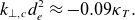 \begin{equation} k_{\perp , c}d_{e}^2 \approx -0.09\kappa _T. \end{equation}
This is the asymptotic slope at $\kappa _T \gg 1$
of the lower solid black line in figure 3.
$\kappa _T \gg 1$
of the lower solid black line in figure 3.
Appendix G. Reduced models of the MDM
In this appendix, we consider two different simplifications of the two-dimensional MDM dispersion relation (3.6). Note that these simplifications are ad hoc in the sense that they cannot be captured by any subsidiary asymptotic expansion of (3.6). Nevertheless, they allow us to understand the qualitative ingredients of our instability.
G.1 The
${\boldsymbol{\nabla }} B$
versus curvature drifts


First, let us discuss the consequences of turning off either the ${\boldsymbol{\nabla }} B$
or curvature drift, starting with the former. Removing the
${\boldsymbol{\nabla }} B$
or curvature drift, starting with the former. Removing the ${\boldsymbol{\nabla }} B$
drift, i.e. the
${\boldsymbol{\nabla }} B$
drift, i.e. the $v_\perp ^2$
-dependent contribution to the magnetic drifts in (C.12), is equivalent to changing the definition of
$v_\perp ^2$
-dependent contribution to the magnetic drifts in (C.12), is equivalent to changing the definition of ${I}_{a,b}$
in (D.20) to
${I}_{a,b}$
in (D.20) to
 \begin{equation} {I}_{a,b}^{(\text{no ${\boldsymbol{\nabla }} B$})} = \frac {1}{\sqrt {\pi }}\int _{-\infty }^{+\infty } \textrm {d} {u}\int _{0}^{+\infty } \textrm {d} {\mu } \frac {\textrm {e}^{-au^2 - b\mu }}{- \zeta + 2\zeta _{\text{d}} u^2} = \frac {1}{b\sqrt {\pi }}\int _{-\infty }^{+\infty } \textrm {d} {u} \frac {\textrm {e}^{-au^2}}{- \zeta + 2\zeta _{\text{d}} u^2}, \end{equation}
where we have explicitly taken the two-dimensional limit discussed in § 3.2. Assuming without loss of generality that $\zeta _{\text{d}} \gt 0$
, we can carry out the integration in (G.1) as
$\zeta _{\text{d}} \gt 0$
, we can carry out the integration in (G.1) as
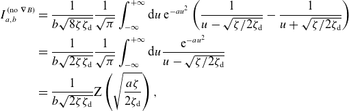 \begin{align} {I}_{a,b}^{(\text{no ${\boldsymbol{\nabla }} B$})} &= \frac {1}{b\sqrt {8\zeta \zeta _{\text{d}}}}\frac {1}{\sqrt {\pi }}\int _{-\infty }^{+\infty } \textrm {d} {u}\, \textrm {e}^{-au^2}\left (\frac {1}{u-\sqrt {\zeta /2\zeta _{\text{d}}}} - \frac {1}{u+\sqrt {\zeta /2\zeta _{\text{d}}}}\right ) \nonumber \\ &= \frac {1}{b\sqrt {2\zeta \zeta _{\text{d}}}}\frac {1}{\sqrt {\pi }}\int _{-\infty }^{+\infty } \textrm {d} {u}\frac { \textrm {e}^{-au^2}}{u-\sqrt {\zeta /2\zeta _{\text{d}}}} \nonumber \\ &= \frac {1}{b\sqrt {2\zeta \zeta _{\text{d}}}} \textrm {Z}\left (\sqrt {\frac {a\zeta }{2\zeta _{\text{d}}}}\right ), \end{align}
where we changed variables $u \mapsto -u$
to go from the first to the second line and then used the definition (3.5) of the plasma dispersion function. Substituting (G.2) into (D.24), we obtain the dispersion relation
$u \mapsto -u$
to go from the first to the second line and then used the definition (3.5) of the plasma dispersion function. Substituting (G.2) into (D.24), we obtain the dispersion relation
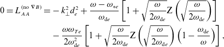 \begin{align} 0 = L_{A A}^{(\text{no ${\boldsymbol{\nabla }} B$})} = &-k_\perp ^2d_{e}^2 + \frac {\omega - \omega _{*{e}}}{\omega _{\text{d}e}}\left [1 + \sqrt {\frac {\omega }{2\omega _{\text{d}e}}}\textrm {Z}\left (\sqrt {\frac {\omega }{2\omega _{\text{d}e}}}\right )\right ] \nonumber \\ &-\frac {\omega \omega _{T{e}}}{2\omega _{\text{d}e}^2} \left [1 + \sqrt {\frac {\omega }{2\omega _{\text{d}e}}}\textrm {Z}\left (\sqrt {\frac {\omega }{2\omega _{\text{d}e}}}\right ) \left (1 - \frac {\omega _{\text{d}e}}{\omega }\right )\right ], \end{align}
where the similarity with (3.6) is evident. The numerical solution of (G.3) shown in figure 8 reveals a good-curvature, viz. $\kappa _T = \omega _{T{e}}/\omega _{\text{d}e} \lt 0$
, instability with the same qualitative behaviour as was seen in figure 3.
$\kappa _T = \omega _{T{e}}/\omega _{\text{d}e} \lt 0$
, instability with the same qualitative behaviour as was seen in figure 3.
In contrast, let us consider turning off the curvature drift, i.e. the $v_\parallel ^2$
-dependent contributions to the magnetic drifts in (C.12). Analogously to (G.1), we find that (D.20) becomes
$v_\parallel ^2$
-dependent contributions to the magnetic drifts in (C.12). Analogously to (G.1), we find that (D.20) becomes
 \begin{equation} {I}_{a,b}^{(\text{no curv})} = \frac {1}{\sqrt {\pi }}\int _{-\infty }^{+\infty } \textrm {d} {u}\int _{0}^{+\infty } \textrm {d} {\mu } \frac {\textrm {e}^{-au^2 - b\mu }}{- \zeta + \zeta _{\text{d}} \mu } = \frac {1}{\zeta _{\text{d}}\sqrt {a}}\int _{0}^{+\infty } \textrm {d} {\mu } \frac {\textrm {e}^{-b\mu }}{\mu - \zeta /\zeta _{\text{d}}}. \end{equation}
Again, we assume that $\zeta _{\text{d}} \gt 0$
. Additionally, we know that (G.4) is an analytic function in the upper half-plane, and so let us look for an alternative integral expression for (G.4) for
$\zeta _{\text{d}} \gt 0$
. Additionally, we know that (G.4) is an analytic function in the upper half-plane, and so let us look for an alternative integral expression for (G.4) for $\text{Re}\:\zeta \lt 0$
that we will later analytically continue to
$\text{Re}\:\zeta \lt 0$
that we will later analytically continue to $\text{Re}\:\zeta \gt 0$
. For
$\text{Re}\:\zeta \gt 0$
. For $\text{Re}\:\zeta \lt 0$
and
$\text{Re}\:\zeta \lt 0$
and $\zeta _{\text{d}} \gt 0$
, we let
$\zeta _{\text{d}} \gt 0$
, we let $\mu = -(t-1) \zeta / \zeta _{\text{d}}$
to find
$\mu = -(t-1) \zeta / \zeta _{\text{d}}$
to find
 \begin{equation} {I}_{a,b}^{(\text{no curv})} = \frac {1}{\zeta _{\text{d}}\sqrt {a}} \exp \left (-\frac {b\zeta }{\zeta _{\text{d}}}\right ) \int _1^{+\infty } \frac {\textrm {d}{t} \,}{t}\exp \left (\frac {b\zeta }{\zeta _{\text{d}}}t\right ) = \frac {1}{\zeta _{\text{d}}\sqrt {a}} \exp \left (-\frac {b\zeta }{\zeta _{\text{d}}}\right ) \textrm {E}_1\left (-\frac {b\zeta }{\zeta _{\text{d}}}\right ), \end{equation}
where $\textrm {E}_1$
is the exponential integral
$\textrm {E}_1$
is the exponential integral
 \begin{equation} \textrm {E}_1(x) \equiv \int _1^{+\infty } \textrm {d}{t} \, \frac {\textrm {e}^{-tx}}{t}. \end{equation}
The function $\textrm {E}_1$
is analytic in the complex plane with a branch cut along the negative real axis. Substituting (G.5) into (D.24), we find the dispersion relation
$\textrm {E}_1$
is analytic in the complex plane with a branch cut along the negative real axis. Substituting (G.5) into (D.24), we find the dispersion relation
 \begin{align} 0 = L_{A A}^{(\text{no curv})} = &-k_\perp ^2d_{e}^2 + \frac {\omega - \omega _{*{e}}}{\omega _{\text{d}e}}\textrm {e}^{-\omega /\omega _{\text{d}e}}\textrm {E}_1\left (\frac {\omega }{\omega _{\text{d}e}}\right ) \nonumber \\ &-\frac {\omega _{T{e}}}{\omega _{\text{d}e}} \left [1 + \frac {\omega }{\omega _{\text{d}e}}\textrm {e}^{-\omega /\omega _{\text{d}e}}\textrm {E}_1\left (\frac {\omega }{\omega _{\text{d}e}}\right )\right ]. \end{align}
To show that this dispersion relation does not contain an MDM-like instability, we consider the simpler case $\omega _{*{e}} = 0$
, wherein, using (G.4)–(G.6), we can express the entirety of (G.7) as
$\omega _{*{e}} = 0$
, wherein, using (G.4)–(G.6), we can express the entirety of (G.7) as
 \begin{equation} \int _{0}^{+\infty } \textrm {d} {\mu } \frac {\mu \textrm {e}^{-\mu }}{\mu - \omega / \omega _{\text{d}e}} = \frac {1 + k_\perp ^2d_{e}^2}{1 - \kappa _T}. \end{equation}
Since the right-hand side of (G.8) is always real, the imaginary part of the left-hand side,
 \begin{equation} \text{Im} \int _{0}^{+\infty } \textrm {d} {\mu } \frac {\mu \textrm {e}^{-\mu }}{\mu - \omega / \omega _{\text{d}e}} = \text{Im}(\omega / \omega _{\text{d}e}) \int _{0}^{+\infty } \textrm {d} {\mu } \frac {\mu \textrm {e}^{-\mu }}{\left \rvert {\mu - \omega / \omega _{\text{d}e}}\right \rvert ^2}, \end{equation}
must vanish. However, (G.9) is non-zero as long as $\text{Im}(\omega ) \gt 0$
.Footnote
16
Therefore, we conclude that the MDM is destabilised exclusively by the curvature drifts.
$\text{Im}(\omega ) \gt 0$
.Footnote
16
Therefore, we conclude that the MDM is destabilised exclusively by the curvature drifts.
This behaviour is drastically different from that of the ETG instability discussed in § 3.2.1. Indeed, analogously to (G.3) and (G.7), we can derive the two-dimensional ETG dispersion relations in the absence of ${\boldsymbol{\nabla }} B$
,
${\boldsymbol{\nabla }} B$
,
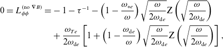 \begin{align} 0 = L_{\phi \phi }^{(\text{no ${\boldsymbol{\nabla }} B$})} = &-1 - \tau ^{-1} - \left (1 - \frac {\omega _{*{e}}}{\omega }\right )\sqrt {\frac {\omega }{2\omega _{\text{d}e}}}\textrm {Z}\left (\sqrt {\frac {\omega }{2\omega _{\text{d}e}}}\right ) \nonumber \\ & + \frac {\omega _{T{e}}}{2\omega _{\text{d}e}}\left [1 + \left (1 - \frac {\omega _{\text{d}e}}{\omega }\right )\sqrt {\frac {\omega }{2\omega _{\text{d}e}}}\textrm {Z}\left (\sqrt {\frac {\omega }{2\omega _{\text{d}e}}}\right )\right ], \end{align}
or of curvature drifts,
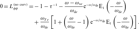 \begin{align} 0 = L_{\phi \phi }^{(\text{no curv})} = &-1 - \tau ^{-1} - \frac {\omega -\omega _{*{e}}}{\omega _{\text{d}e}}\textrm {e}^{-\omega /\omega _{\text{d}e}}\textrm {E}_1\left (-\frac {\omega }{\omega _{\text{d}e}}\right ) \nonumber \\ &+ \frac {\omega _{T{e}}}{\omega _{\text{d}e}} \left [1 + \left (\frac {\omega }{\omega _{\text{d}e}} - 1\right )\textrm {e}^{-\omega /\omega _{\text{d}e}}\textrm {E}_1\left (-\frac {\omega }{\omega _{\text{d}e}}\right )\right ]. \end{align}
Expanding in the strongly driven ( $\omega _{\text{d}e} \ll \omega \ll \omega _{T{e}}$
), zero-density-gradient (
$\omega _{\text{d}e} \ll \omega \ll \omega _{T{e}}$
), zero-density-gradient ( $\omega _{*{e}} = 0$
) limit considered in § 3.2.1, we find that both (G.10) and (G.11) yield
$\omega _{*{e}} = 0$
) limit considered in § 3.2.1, we find that both (G.10) and (G.11) yield
 \begin{equation} \omega ^2 = -\omega _{T{e}} \omega _{\text{d}e}\tau . \end{equation}
This dispersion relation can also be obtained directly from (3.10)–(3.12) by noticing that dropping the ${\boldsymbol{\nabla }} B$
drift simplifies the fluid equations to
${\boldsymbol{\nabla }} B$
drift simplifies the fluid equations to
 \begin{align} &\frac {\partial }{\partial t}\frac {\delta n_{e{\boldsymbol{k}}}}{{n_{e}}} + \textrm {i}\omega _{\text{d}e}\frac {\delta T_{\parallel {e}{\boldsymbol{k}}}}{T_{e}} = 0, \\[-12pt] \nonumber \end{align}
 \begin{align} &\frac {\partial }{\partial t}\frac {\delta T_{\parallel {e}{\boldsymbol{k}}}}{T_{e}} + \textrm {i}\omega _{T{e}}\frac {e{\phi }_{\boldsymbol{k}}}{T_{e}} = 0, \\[6pt] \nonumber \end{align}
whereas dropping the curvature drift yields
 \begin{align} &\frac {\partial }{\partial t}\frac {\delta n_{e{\boldsymbol{k}}}}{{n_{e}}} + \textrm {i}\omega _{\text{d}e}\frac {\delta T_{\perp {e}{\boldsymbol{k}}}}{T_{e}} = 0, \end{align}
 \begin{align} &\frac {\partial }{\partial t}\frac {\delta T_{\perp {e}{\boldsymbol{k}}}}{T_{e}} + \textrm {i}\omega _{T{e}}\frac {e{\phi }_{\boldsymbol{k}}}{T_{e}} = 0. \\[6pt] \nonumber \end{align}
In either case, we obtain the dispersion relation (G.12). This confirms that the curvature-driven ETG instability is indifferent to which magnetic drift couples the density and temperature fluctuations.
G.2 Colliding beams
Possibly the simplest version of the MDM can be obtained if we make the unphysical assumption that the unperturbed distribution function is
 \begin{equation} F_{e} = \frac {1}{2}{n_{e}} \delta (v_x)\delta (v_y) \left [\delta (v_\parallel - v_0) + \delta (v_\parallel + v_0)\right ], \end{equation}
where $v_0 = v_0(x)$
can be thought of as a spatially varying thermal speed: by definition,
$v_0 = v_0(x)$
can be thought of as a spatially varying thermal speed: by definition,
 \begin{equation} \frac {1}{2}v_{\text{th}{e}}^2 = \frac {1}{{n_{e}}}\int \textrm {d}^{3} \boldsymbol{v}\, v^2 F_{e} = v_0^2. \end{equation}
The temperature-gradient length scale (2.14) is then
 \begin{equation} \frac {1}{L_{T_{e}}} = -2 \frac {\textrm {d}\,{\ln v_0}}{\textrm {d}{x}}. \end{equation}
The distribution function (G.17) is made up of two counter-propagating beams aligned with the $z$
direction, with zero net momentum but radially varying energy. Such a distribution function is entirely unphysical in the sense that it would give rise to high-frequency instabilities that are outside the ordering (2.1). In other words, (G.17) is not a valid GK equilibrium distribution. Nevertheless, we can use it as an ad hoc toy model for the MDM.
$z$
direction, with zero net momentum but radially varying energy. Such a distribution function is entirely unphysical in the sense that it would give rise to high-frequency instabilities that are outside the ordering (2.1). In other words, (G.17) is not a valid GK equilibrium distribution. Nevertheless, we can use it as an ad hoc toy model for the MDM.

Note that the last term in the odd (in $v_\parallel$
) drift-kinetic equation (C.16) comes from the last term in (2.4), and thus (C.16) is
$v_\parallel$
) drift-kinetic equation (C.16) comes from the last term in (2.4), and thus (C.16) is
 \begin{align} &\frac {\partial }{\partial t} \left ({h}_{{e}{\boldsymbol{k}}}^{\text{(odd)}} - \frac {2v_\parallel }{v_{\text{th}{e}}}\frac {\delta {A}_{\parallel {\boldsymbol{k}}}}{\rho _{e} B} F_{e} \right ) + \textrm {i} \omega _{\text{d}e}\left (\frac {2v_\parallel ^2}{v_{\text{th}{e}}^2} + \frac {v_\perp ^2}{v_{\text{th}{e}}^2}\right ){h}_{{e}{\boldsymbol{k}}}^{\text{(odd)}}+ \textrm {i} k_y \frac {\rho _{e}v_{\text{th}{e}}}{2} \frac {2v_\parallel }{v_{\text{th}{e}}}\frac {\delta {A}_{\parallel {\boldsymbol{k}}}}{\rho _{e} B} \frac {\textrm {d}{F_{e}}}{\textrm {d}{x}} = 0. \end{align}
Substituting (G.17) instead of a Maxwellian $F_{e}$
into (G.20), we find that the odd drift-kinetic equation for a mode with complex frequency
$F_{e}$
into (G.20), we find that the odd drift-kinetic equation for a mode with complex frequency $\omega$
is
$\omega$
is
 \begin{align} &-\omega \left ({h}_{{e}{\boldsymbol{k}}}^{\text{(odd)}} - \frac {2v_\parallel }{v_{\text{th}{e}}}\frac {\delta {A}_{\parallel {\boldsymbol{k}}}}{\rho _{e} B} F_{e} \right ) + \omega _{\text{d}e}\left (\frac {2v_\parallel ^2}{v_{\text{th}{e}}^2} + \frac {v_\perp ^2}{v_{\text{th}{e}}^2}\right ){h}_{{e}{\boldsymbol{k}}}^{\text{(odd)}} - \omega _{*{e}} \frac {2v_\parallel }{v_{\text{th}{e}}}\frac {\delta {A}_{\parallel {\boldsymbol{k}}}}{\rho _{e} B}F_{e}\nonumber \\ &\quad - \omega _{T{e}} \frac {2v_\parallel }{v_{\text{th}{e}}}\frac {\delta {A}_{\parallel {\boldsymbol{k}}}}{\rho _{e} B} \frac {{n_{e}} v_0}{4} \delta (v_x)\delta (v_y) \frac {\partial }{\partial {v_\parallel }} \left [\delta (v_\parallel - v_0) - \delta (v_\parallel + v_0)\right ] = 0. \end{align}
Substituting ${h}_{{e}{\boldsymbol{k}}}^{\text{(odd)}}$
from (G.21) into Ampère’s law (C.14), we obtain the following dispersion relation:
${h}_{{e}{\boldsymbol{k}}}^{\text{(odd)}}$
from (G.21) into Ampère’s law (C.14), we obtain the following dispersion relation:
 \begin{equation} -k_\perp ^2d_{e}^2 - \frac {\omega -\omega _{*{e}} -\omega _{T{e}}}{\omega - \omega _{\text{d}e}} + \frac {\omega _{T{e}}\omega _{\text{d}e}}{(\omega - \omega _{\text{d}e})^2} = 0. \end{equation}
It is straightforward to show that (G.22) has unstable solutions when
 \begin{equation} (\kappa _n + \kappa _T - 1)^2 + 4\kappa _T (1+k_\perp ^2d_{e}^2) \lt 0, \end{equation}
which is possible only if $\kappa _T \lt 0$
. Note that in the case of zero magnetic drifts, viz.
$\kappa _T \lt 0$
. Note that in the case of zero magnetic drifts, viz. $\omega _{\text{d}e} = 0$
, (G.22) reproduces the magnetic drift wave (3.22).
$\omega _{\text{d}e} = 0$
, (G.22) reproduces the magnetic drift wave (3.22).
Figure 9 shows the unstable solutions of (G.22) for the same parameters as figures 3 and 8. The qualitative similarity between these is evident, in particular the fact that the unstable solutions of (G.22) can have either sign of $\text{Re}\:\omega$
. The main difference is that, in the limit
$\text{Re}\:\omega$
. The main difference is that, in the limit $k_\perp ^2d_{e}^2 \gg 1$
, the stability boundary associated with the
$k_\perp ^2d_{e}^2 \gg 1$
, the stability boundary associated with the $\text{Re}\:\omega \gt 0$
, i.e. copropagating, modes asymptotes to
$\text{Re}\:\omega \gt 0$
, i.e. copropagating, modes asymptotes to $\kappa _T \to 0^-$
, as can be seen directly from (G.23). This is consistent with the hypothesis that the stabilisation of the MDM at positive real frequency is due to the Landau-like damping arising from the magnetic drifts. The discontinuous nature of the distribution function (G.17) implies that only a single
$\kappa _T \to 0^-$
, as can be seen directly from (G.23). This is consistent with the hypothesis that the stabilisation of the MDM at positive real frequency is due to the Landau-like damping arising from the magnetic drifts. The discontinuous nature of the distribution function (G.17) implies that only a single $\omega$
, viz.
$\omega$
, viz. $\omega =\omega _{\text{d}e}$
, is resonant, unlike in the continuous case, where every
$\omega =\omega _{\text{d}e}$
, is resonant, unlike in the continuous case, where every $\omega \gt 0$
resonates with some particles.
$\omega \gt 0$
resonates with some particles.


 Open access