


1. Introduction
Taylor–Aris dispersion describes the enhanced spreading of solute in a fluid due to the coupled effects of advection and diffusion. G. I. Taylor (Reference Taylor1953) first developed an analytical solution for the long-term dispersive behaviour of solute based largely on the idea that the radial diffusion (i.e. transverse to flow) approximately balances axial dispersion caused by the non-uniform velocity field. The analysis was later formalised and significantly extended by Aris (Reference Aris1956). Aris introduced a solution method that is now called the method of moments (MoM). The MoM reformulates the dispersion problem in terms of axial integrals of the concentration field which correspond to, for example, the axial mean and variance of the solute zone. Generally, Taylor–Aris dispersion is highly relevant to a wide variety of applications, ranging from analytical chemistry to microfluidics and to large-scale environmental flows (Brenner & Edwards Reference Brenner and Edwards1993).
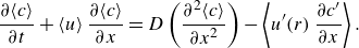
Taylor’s original analysis, focused on classic pressure-driven flow (PDF) in a cylindrical tube, provided a closed-form solution for solute dispersion for a regime that can be summarised as $L/a\gg P\hspace{0pt}e\gg 6.9$
. Here,
$L/a\gg P\hspace{0pt}e\gg 6.9$
. Here, $L$
is an axial distance of travel of the solute,
$L$
is an axial distance of travel of the solute, $a$
is the inner radius of the tube and
$a$
is the inner radius of the tube and $P\hspace{0pt}e$
is a Péclet number (
$P\hspace{0pt}e$
is a Péclet number ( $a\langle u\rangle /D$
where
$a\langle u\rangle /D$
where $D$
is the molecular diffusivity) based on
$D$
is the molecular diffusivity) based on $a$
and the area-averaged bulk velocity
$a$
and the area-averaged bulk velocity $\langle u\rangle$
(the brackets indicate a cross-sectional area average). This condition implies that the advective time scale,
$\langle u\rangle$
(the brackets indicate a cross-sectional area average). This condition implies that the advective time scale, $L/\langle u\rangle$
, is large relative to the characteristic time of transverse diffusion,
$L/\langle u\rangle$
, is large relative to the characteristic time of transverse diffusion, $a^{2}/D$
, which we will here refer to as the ‘long-time limit’ or the ‘quasi-steady’ regime of the problem. Aris (Reference Aris1956) subsequently expanded upon G. I. Taylor’s work in several important ways. First, he included the effects of axial molecular diffusion for the quasi-steady problem. Aris also generalised the problem and introduced the MoM as a mathematical framework that enables the analysis of solute dispersion across all time regimes, starting from arbitrary initial conditions. Aris’ MoM is applicable to channels of arbitrary cross-sectional geometries and, relevant here, to arbitrary velocity fields. Taylor’s analysis and Aris’ model in the quasi-steady (long-time) regime predict that the area-averaged concentration of the solute will reach an axial Gaussian distribution that has a variance which grows linearly with time. This linear growth can be characterised by an effective dispersion coefficient.
$a^{2}/D$
, which we will here refer to as the ‘long-time limit’ or the ‘quasi-steady’ regime of the problem. Aris (Reference Aris1956) subsequently expanded upon G. I. Taylor’s work in several important ways. First, he included the effects of axial molecular diffusion for the quasi-steady problem. Aris also generalised the problem and introduced the MoM as a mathematical framework that enables the analysis of solute dispersion across all time regimes, starting from arbitrary initial conditions. Aris’ MoM is applicable to channels of arbitrary cross-sectional geometries and, relevant here, to arbitrary velocity fields. Taylor’s analysis and Aris’ model in the quasi-steady (long-time) regime predict that the area-averaged concentration of the solute will reach an axial Gaussian distribution that has a variance which grows linearly with time. This linear growth can be characterised by an effective dispersion coefficient.
While neither Taylor nor Aris rigorously analysed the early variance growth of the solute zone, Barton (Reference Barton1983) significantly extended Aris’ MoM to analyse solute behaviour across time regimes and for arbitrary velocity fields. In particular, Barton derived general expressions for the first three integral moments of the concentration field, valid in all time regimes. In the same paper, Barton applied his work to three specific flow profiles and geometries for select initial conditions: plane Couette flow, Poiseuille flow in a cylindrical tube and an analytical approximation of turbulent channel flow.
Gill & Sankarasubramanian (Reference Gill and Sankarasubramanian1970, Reference Gill and Sankarasubramanian1971) developed a distinct yet related approach to the MoM to describe solute concentration in a manner valid across all time regimes. They formulated the solute concentration field as an infinite series of axial derivatives of the area-averaged solute concentration, a method known as a Kramers–Moyal-type expansion. The dispersion coefficients, which correspond to the integral moments of the solute distribution, emerge naturally as the eigenvalues of this solution ansatz. Since Gill & Sankarasubramanian’s work, Chatwin (Reference Chatwin1970, Reference Chatwin1972), Degance & Johns (Reference Degance and Johns1978a ,Reference Degance and Johns b ), Mauri (Reference Mauri1991) and Wang & Chen (Reference Wang and Chen2016) extended this Kramers–Moyal-type solution method to various dispersion problems. For a detailed discussion of Kramers–Moyal-type expansions and other pre-asymptotic solution methods, see Taghizadeh, Valdés-Parada & Wood (Reference Taghizadeh, Valdés-Parada and Wood2020). Note that Aris and Barton’s MoM (which we leverage in our analysis in § 4) is a largely different approach to solving dispersion problems than Gill’s Kramers–Moyal-type expansions. The MoM produces one partial and one ordinary differential equation (per moment) that govern the nth integral moment of the concentration field. These equations can often be solved directly by techniques such as eigenfunction expansions or Laplace transforms. In contrast, Gill’s method derives dispersion coefficients as eigenvalues of a Kramers–Moyal expansion of the solute concentration field. However, both solution methods involve deriving expressions for either the nth moment of the concentration field (MoM) or the nth dispersion coefficient (Kramers–Moyal), whence constructing a formulation for the (n+1)st and (n+2)nd moment or coefficient. Both processes therefore generate equations that build on others to describe progressively higher-order moments.
Several other solution methods have been developed for these problems which further extend the mathematical and physical understanding of solute dispersion. Brenner (Reference Brenner1980) generalised Aris’ framework by analysing the so-called local and total moments of the probability density function of a tracer particle in a spatially periodic cell. Brenner demonstrated that the solution of various moments can be obtained by solving the elliptical partial differential equation of a cell field $\boldsymbol{B}$
defined on an individual period cell. The solution can be used to compute a tensor that characterises the long-term dispersion behaviour of solutes. Brenner’s approach, known as the Brenner–Aris theory or the macrotransport paradigm, provides a very broad framework for understanding transport phenomena in heterogeneous systems, such as porous media.
$\boldsymbol{B}$
defined on an individual period cell. The solution can be used to compute a tensor that characterises the long-term dispersion behaviour of solutes. Brenner’s approach, known as the Brenner–Aris theory or the macrotransport paradigm, provides a very broad framework for understanding transport phenomena in heterogeneous systems, such as porous media.
Mercer & Roberts (Reference Mercer and Roberts1990) pioneered the use of infinite-dimensional centre manifold theory in the analysis of Taylor dispersion by obtaining higher-order asymptotic approximations for the classic, Taylor-type diffusive model. In a significant development, Balakotaiah & Chang (Reference Balakotaiah and Chang1995) applied centre manifold theory to flows with additional complexities, such as bulk reactions, surface reactions, adsorption and desorption and transverse velocity gradients. Rosencrans (Reference Rosencrans1997) further extended the use of centre manifold theory to dispersion in channels with slow axial variations in width.
Later, Stone & Brenner (Reference Stone and Brenner1999) formalised and extended Taylor’s (Reference Taylor1953) original solution method. Stone & Brenner introduced a more organised set of assumptions for the problem, more intuitive notation (which we will here adopt) and extended the solution to velocity fields which slowly vary in the axial direction. Consistent with the original Taylor analysis, Stone & Brenner’s solution method is valid for the long-time limit of the problem.
Beyond advancements in solution methods, much effort has been devoted to analysing dispersion in varying channel geometries and for a variety of velocity fields. We here focus on dispersion in electrokinetic phenomena in a cylindrical tube. Specifically, electroosmotic flow (EOF) plays a pivotal role in analytical chemistry processes and electrokinetic microfluidic applications. Electroosmotic flow refers to the bulk flow of a liquid induced by an externally applied electric field imparting Coulombic forces on the diffuse charges of electric double layers (EDLs; Hunter Reference Hunter1988). These EDLs form spontaneously on the wetted walls of a liquid-filled channel. Electroosmotic flow is inherently applicable to small (micron- and nanometre-scale) channels and offers electrical control of flow and solutes in devices with no moving parts. The Poisson–Boltzmann equation describes the electric potential throughout a tube caused by the EDL. The most common approximate solution to the latter is the Debye–Hückel approximation, which assumes low zeta potential ( $\zeta \lt 25.7\text{ mV}$
at room temperature; Probstein Reference Probstein1994, p. 193). Here, the zeta potential is defined as the electric potential at the shear plane (where the no-slip condition is applied). Using the Debye–Hückel approximation, Rice & Whitehead (Reference Rice and Whitehead1965) first described the EOF profile in a cylindrical tube by solving the steady Stokes equation for a Newtonian fluid. Given the linearity of the Stokes equation, the EOF profile is simply (arithmetically) superposable with PDF. Since Rice & Whitehead’s paper, many researchers have examined EOF velocity fields in a variety of contexts. This includes work in cylindrical channels with high zeta potentials (Levine et al. Reference Levine, Marriott, Neale and Epstein1975), channels with axially varying zeta potentials (Anderson & Idol Reference Anderson and Idol1985), porous media (Coelho et al. Reference Coelho, Shapiro, Thovert and Adler1996; Gupta, Coelho & Adler Reference Gupta, Coelho and Adler2006), annular geometries with both low (Tsao Reference Tsao2000) and finite (Kang, Yang & Huang Reference Kang, Yang and Huang2002) zeta potentials and rectangular channels (Wang et al. Reference Wang, Wong, Yang and Ooi2007; Mondal, Misra & De Reference Mondal, Misra and De2014). Additionally, note that applying a pressure gradient to a channel can cause a streaming potential to form (Scales et al. Reference Scales, Grieser, Healy, White and Chan1992). If substantial, this streaming potential can induce some amount of EOF. Hence, understanding the behaviour of EOF can be important even in the absence of an externally applied electric field, particularly in channels with thick EDLs relative to the channel radius (Kim & Kim Reference Kim and Kim2018; Riad, Khorshidi & Sadrzadeh Reference Riad, Khorshidi and Sadrzadeh2020).
$\zeta \lt 25.7\text{ mV}$
at room temperature; Probstein Reference Probstein1994, p. 193). Here, the zeta potential is defined as the electric potential at the shear plane (where the no-slip condition is applied). Using the Debye–Hückel approximation, Rice & Whitehead (Reference Rice and Whitehead1965) first described the EOF profile in a cylindrical tube by solving the steady Stokes equation for a Newtonian fluid. Given the linearity of the Stokes equation, the EOF profile is simply (arithmetically) superposable with PDF. Since Rice & Whitehead’s paper, many researchers have examined EOF velocity fields in a variety of contexts. This includes work in cylindrical channels with high zeta potentials (Levine et al. Reference Levine, Marriott, Neale and Epstein1975), channels with axially varying zeta potentials (Anderson & Idol Reference Anderson and Idol1985), porous media (Coelho et al. Reference Coelho, Shapiro, Thovert and Adler1996; Gupta, Coelho & Adler Reference Gupta, Coelho and Adler2006), annular geometries with both low (Tsao Reference Tsao2000) and finite (Kang, Yang & Huang Reference Kang, Yang and Huang2002) zeta potentials and rectangular channels (Wang et al. Reference Wang, Wong, Yang and Ooi2007; Mondal, Misra & De Reference Mondal, Misra and De2014). Additionally, note that applying a pressure gradient to a channel can cause a streaming potential to form (Scales et al. Reference Scales, Grieser, Healy, White and Chan1992). If substantial, this streaming potential can induce some amount of EOF. Hence, understanding the behaviour of EOF can be important even in the absence of an externally applied electric field, particularly in channels with thick EDLs relative to the channel radius (Kim & Kim Reference Kim and Kim2018; Riad, Khorshidi & Sadrzadeh Reference Riad, Khorshidi and Sadrzadeh2020).
The interplay between EOF and PDF introduces interesting flow dynamics that significantly affect solute dispersion. Datta & Kotamarthi (Reference Datta and Kotamarthi1990) first analysed Taylor–Aris dispersion for coupled EOF and PDF in cylindrical tubes, deriving an effective dispersion coefficient under long-time regimes. They also identified the optima of both the flow Péclet number and the relative magnitudes of PDF and EOF to minimise the theoretical plate height (Huang Reference Huang2021). However, Datta & Kotamarthi’s (Reference Datta and Kotamarthi1990) work had several limitations. For example, they did not present a derivation of their effective dispersion coefficient. They offered no benchmarking with other models (such as computational fluid dynamics models of dispersion or Brownian dynamics simulations). Datta & Kotamarthi (Reference Datta and Kotamarthi1990) also focused exclusively on the long-time (quasi-steady) regime. Griffiths & Nilson (Reference Griffiths and Nilson1999) later presented the coefficient of effective dispersion for pure EOF in both cylindrical tubes (a special case of Datta & Kotamarthi’s model) and a flow between large parallel plates. For both geometries, Griffiths & Nilson (Reference Griffiths and Nilson1999) considered the case of low zeta potential. Griffiths & Nilson (Reference Griffiths and Nilson1999) used an asymptotic method rather than the area-averaging method of Stone & Brenner (Reference Stone and Brenner1999), yet they considered a solution that is valid only in long-time regimes. Griffiths & Nilson (Reference Griffiths and Nilson2000) later generalised their models with numerical solutions to account for large zeta potentials. Zholkovskij, Masliyah & Czarnecki (Reference Zholkovskij, Masliyah and Czarnecki2003) subsequently analysed the long-term dispersive behaviour of solute under pure EOF in a channel with an arbitrary cross-section. Further analyses by Dutta & Leighton (Reference Dutta and Leighton2003) and Zholkovskij & Masliyah (Reference Zholkovskij and Masliyah2004) examined the effects of channel geometries on dispersion in coupled EOF and PDF, again focusing only on long-time regimes. Dutta (Reference Dutta2007) later investigated dispersion caused by EOF in a rectangular channel with low zeta potential. Thereafter, Paul & Ng (Reference Paul and Ng2012) analysed dispersion in pure EOF in a rectangular channel under low zeta potential across all time regimes.
More recent studies of solute dispersion have continued to focus largely on the long-term limit of the problem. For example, Dejam, Hassanzadeh & Chen (Reference Dejam, Hassanzadeh and Chen2015) examined dispersion in combined EOF and PDF in porous channels, while Hoshyargar et al. (Reference Hoshyargar, Talebi, Ashrafizadeh and Sadeghi2018) analysed the effects of viscoelastic fluids on dispersion, both in long-time regimes. Thus, most of the literature regarding Taylor–Aris dispersion of combined EOF and PDF is applicable only in physical regimes where $\textit{Pe}\lt \lt \sigma _{x}/a$
, where
$\textit{Pe}\lt \lt \sigma _{x}/a$
, where $\sigma _{x}$
is the characteristic width of the solute zone. This limitation is particularly important as microfluidic transport is oftentimes rapid enough that this quasi-steady regime does not apply (Stone & Kim Reference Stone and Kim2001). Lastly, we note that Taylor-type analysis also offers an approximation of the radial distribution of solute, and this radial distribution has never been addressed for neither EOF nor combined EOF and PDF.
$\sigma _{x}$
is the characteristic width of the solute zone. This limitation is particularly important as microfluidic transport is oftentimes rapid enough that this quasi-steady regime does not apply (Stone & Kim Reference Stone and Kim2001). Lastly, we note that Taylor-type analysis also offers an approximation of the radial distribution of solute, and this radial distribution has never been addressed for neither EOF nor combined EOF and PDF.
To our knowledge, all previous analyses of Taylor dispersion for coupled EOF and PDF focused on the long-term dispersion behaviour and were not able to provide a prediction of both the short- and long-term evolution of the solute zone. In the current study, we address this by presenting a more comprehensive analysis of Taylor–Aris dispersion for coupled EOF and PDF in cylindrical tubes. We first derive an expression for the EOF velocity profile that is valid for an EDL of arbitrary thickness relative to the channel radius. We then present a long-time analysis of the solute dispersion. To our knowledge, this is the first presentation of such a derivation and first analysis of the radial component of the resulting distribution. We next apply the MoM to analyse dispersion conditions across all time regimes. To this end, we derive the first two integral moments of the solute zone and examine specific initial conditions of solute. We benchmark both our Taylor-type and MoM formulations against Brownian dynamics simulations for a broad range of cases, including various time scales; flow Péclet numbers; relative magnitudes of EOF versus PDF; and tube radii relative to the Debye length. Finally, we present methods and analytical expressions useful in minimising dispersion for combined PDF and EOF in all time regimes. Specifically, we find optima associated with the relative magnitudes of EOF and PDF and the optimal Péclet number to minimise band broadening across all time regimes.
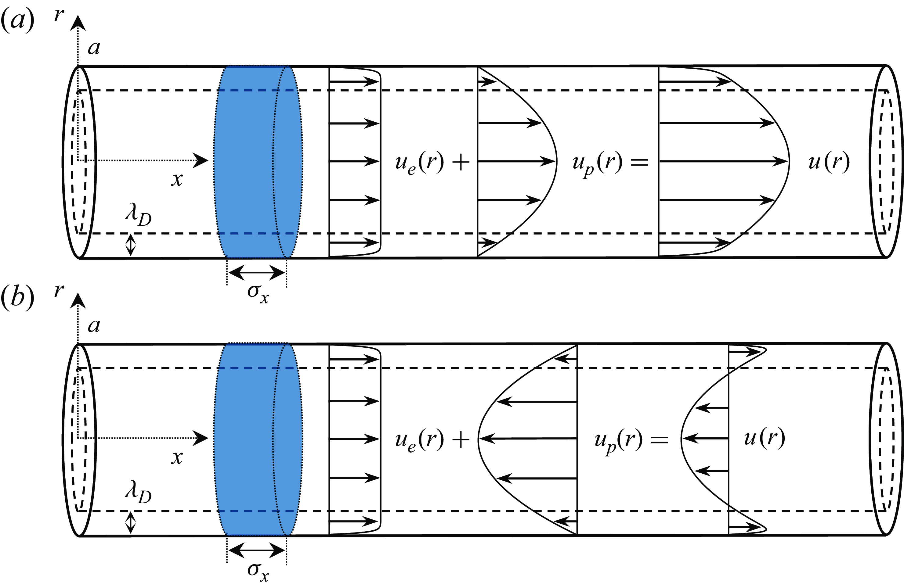
Schematics of a solute transported in a cylindrical tube of inner radius a under a combination of PDF and EOF. A solute zone of characteristic length of $\sigma _{x}$
is subjected to a flow consisting of combinations of steady PDF,
$\sigma _{x}$
is subjected to a flow consisting of combinations of steady PDF, $u_{p}(r)$
, and steady EOF,
$u_{p}(r)$
, and steady EOF, $u_{e}(r)$
, (with finite EDL thickness) along the axial direction,
$u_{e}(r)$
, (with finite EDL thickness) along the axial direction, $x$
.
$x$
. $(a)$
Pressure-driven flow and EOF in the same direction.
$(a)$
Pressure-driven flow and EOF in the same direction. $(b)$
Pressure-driven flow in opposition to EOF. The resulting net flow profile is denoted as
$(b)$
Pressure-driven flow in opposition to EOF. The resulting net flow profile is denoted as $u(r)$
, and Debye length is denoted as
$u(r)$
, and Debye length is denoted as $\lambda _{D}$
. Both the tube radius and Debye length are depicted enlarged relative to the axial length of the tube for clarity of presentation.
$\lambda _{D}$
. Both the tube radius and Debye length are depicted enlarged relative to the axial length of the tube for clarity of presentation.
2. Formulation of the basic flow and solute transport problem
2.1. Flow field and basic problem description
We study the flow and dispersion of a neutral (uncharged) solute subject to simultaneous PDF and EOF in a cylindrical tube of inner radius $a\,.$
Figure 1 shows schematics of an initial condition of the solute and example flow profiles. The flow is generated from applied axial pressure differentials (resulting in a Poiseuille-type flow component, see, e.g. Langlois & Deville Reference Langlois and Deville2014) and/or by EOF caused by the presence of a finite sized EDL at the wetted wall and an electric field applied along the axis of the tube. The EDL may or may not overlap with itself at the centre of the tube (see Appendix A). We will denote the characteristic axial width of the solute zone as
$a\,.$
Figure 1 shows schematics of an initial condition of the solute and example flow profiles. The flow is generated from applied axial pressure differentials (resulting in a Poiseuille-type flow component, see, e.g. Langlois & Deville Reference Langlois and Deville2014) and/or by EOF caused by the presence of a finite sized EDL at the wetted wall and an electric field applied along the axis of the tube. The EDL may or may not overlap with itself at the centre of the tube (see Appendix A). We will denote the characteristic axial width of the solute zone as $\sigma _{x}$
and assume the solute is of uniform molecular diffusivity (
$\sigma _{x}$
and assume the solute is of uniform molecular diffusivity ( $D$
) throughout the tube. The Debye length is denoted as
$D$
) throughout the tube. The Debye length is denoted as $\lambda _{D}$
. Let
$\lambda _{D}$
. Let $r^{*}=r/a$
denote the dimensionless radial coordinate and
$r^{*}=r/a$
denote the dimensionless radial coordinate and $\phi =a/\lambda _{D}$
be the tube radius scaled by Debye length. For EOF, we consider a general electrolyte and a wall zeta potential sufficiently weak such that the Debye–Hückel approximation holds (Probstein Reference Probstein1994). We will further neglect the effects of streaming potential on the fluid velocity field. Note the latter effects should not create new shapes of the velocity field but may introduce a coupling between EOF and PDF which is not explicitly treated here. We provide a derivation of the electric potential field and EOF velocity profile, valid for an EDL of arbitrary thickness relative to the channel radius, in Appendix A. From (A11), the electric potential field within the tube is given by
$\phi =a/\lambda _{D}$
be the tube radius scaled by Debye length. For EOF, we consider a general electrolyte and a wall zeta potential sufficiently weak such that the Debye–Hückel approximation holds (Probstein Reference Probstein1994). We will further neglect the effects of streaming potential on the fluid velocity field. Note the latter effects should not create new shapes of the velocity field but may introduce a coupling between EOF and PDF which is not explicitly treated here. We provide a derivation of the electric potential field and EOF velocity profile, valid for an EDL of arbitrary thickness relative to the channel radius, in Appendix A. From (A11), the electric potential field within the tube is given by $\psi (r^{*})=\zeta I_{0}(\phi r^{*})/I_{0}(\phi )$
, where
$\psi (r^{*})=\zeta I_{0}(\phi r^{*})/I_{0}(\phi )$
, where $I_{0}(z)$
is a zeroth-order modified Bessel function of the first kind and
$I_{0}(z)$
is a zeroth-order modified Bessel function of the first kind and $\zeta$
is the zeta potential. Further, from (A14), the EOF velocity profile can be expressed as
$\zeta$
is the zeta potential. Further, from (A14), the EOF velocity profile can be expressed as $u_{e}(r^{*})=u_{\textit{HS}}(1-\psi (r^{*})/\zeta )$
where
$u_{e}(r^{*})=u_{\textit{HS}}(1-\psi (r^{*})/\zeta )$
where $u_{\textit{HS}}=-\varepsilon _{e}E\zeta /\mu$
is the Helmholtz–Smoluchowski velocity scale. Here,
$u_{\textit{HS}}=-\varepsilon _{e}E\zeta /\mu$
is the Helmholtz–Smoluchowski velocity scale. Here, $\varepsilon _{e}$
is the permittivity of the fluid (assumed to be uniform throughout the tube),
$\varepsilon _{e}$
is the permittivity of the fluid (assumed to be uniform throughout the tube), $E$
is the magnitude of the applied electric field and
$E$
is the magnitude of the applied electric field and $\mu$
is the dynamic viscosity of the fluid. For a compact notation, we define the following dimensionless cross-sectional average of the radial electric potential:
$\mu$
is the dynamic viscosity of the fluid. For a compact notation, we define the following dimensionless cross-sectional average of the radial electric potential:
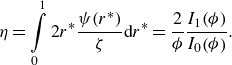 \begin{equation} \eta =\int \limits_{0}^{1}2r^{*}\frac{\psi\!\left(r^{*}\right)}{\zeta }\mathrm{d}r^{*}=\frac{2}{\phi }\frac{I_{1}\!\left(\phi \right)}{I_{0}\!\left(\phi \right)} .\end{equation}
Taking the area average of the EOF profile
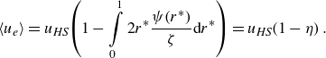 \begin{equation} \left\langle u_{e}\right\rangle =u_{\textit{HS}}\!\left(1-\int\limits _{0}^{1}2r^{*}\frac{\psi\!\left(r^{*}\right)}{\zeta }\mathrm{d}r^{*}\right)=u_{\textit{HS}}\!\left(1-\eta \right) .\end{equation}
Further, for the case of a thick EDL relative to the tube radius ( $\phi \ll 1$
), we can expand
$\phi \ll 1$
), we can expand $I_{0}$
using a Taylor series expansion. Neglecting terms of order
$I_{0}$
using a Taylor series expansion. Neglecting terms of order $O[\phi ^{4}]$
and higher, we can approximate
$O[\phi ^{4}]$
and higher, we can approximate
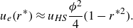 \begin{equation} u_{e} (r^{*})\approx u_{\textit{HS}}\frac{\phi ^{2}}{4} \big(1-r^{*2}\big) .\end{equation}
Thus, as the EDL becomes thicker relative to the radius of the channel, EOF tends to a parabolic profile, and $\phi$
informs the bulk velocity of the flow.
$\phi$
informs the bulk velocity of the flow.
The PDF profile is given as $u_{p}(r^{*})=2\langle u_{p}\rangle (1-r^{*2})$
with
$u_{p}(r^{*})=2\langle u_{p}\rangle (1-r^{*2})$
with $\langle u_{p}\rangle$
denoting the area-averaged PDF profile. A tube subject to both pressure gradients and EOF has a net velocity profile given by
$\langle u_{p}\rangle$
denoting the area-averaged PDF profile. A tube subject to both pressure gradients and EOF has a net velocity profile given by $u(r^{*})=u_{e}(r^{*})+u_{p}(r^{*})$
. Combining with (2.2), we can express the full velocity profile as
$u(r^{*})=u_{e}(r^{*})+u_{p}(r^{*})$
. Combining with (2.2), we can express the full velocity profile as
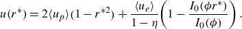 \begin{equation} u(r^{*})=2\langle u_{p}\rangle \big(1-r^{*2}\big)+\frac{\left\langle u_{e}\right\rangle }{1-\eta }\!\left(1-\frac{I_{0}\!\left(\phi r^{*}\right)}{I_{0}\!\left(\phi \right)}\right) .\end{equation}
The area average of (2.4) is simply $\langle u\rangle =\langle u_{e}\rangle +\langle u_{p}\rangle$
. Lastly, we take the deviation from this area average as
$\langle u\rangle =\langle u_{e}\rangle +\langle u_{p}\rangle$
. Lastly, we take the deviation from this area average as
 \begin{equation} u^{\prime} (r^{*})=u(r^{*})- \langle u \rangle = \langle u_{p} \rangle \big(1-2r^{*2}\big)+\frac{\left\langle u_{e}\right\rangle }{1-\eta }\!\left(\eta -\frac{I_{0}\!\left(\phi r^{*}\right)}{I_{0}\!\left(\phi \right)}\right) .\end{equation}
Figure 1(a) shows a flow profile where PDF and EOF are in the same direction, corresponding to values of $\langle u_{p}\rangle \gt 0$
and
$\langle u_{p}\rangle \gt 0$
and $\langle u_{e}\rangle \gt 0$
. Figure 1(b) shows a flow profile where EOF is opposed by PDF, corresponding to values of
$\langle u_{e}\rangle \gt 0$
. Figure 1(b) shows a flow profile where EOF is opposed by PDF, corresponding to values of $\langle u_{p}\rangle \lt 0\lt \langle u_{e}\rangle$
.
$\langle u_{p}\rangle \lt 0\lt \langle u_{e}\rangle$
.
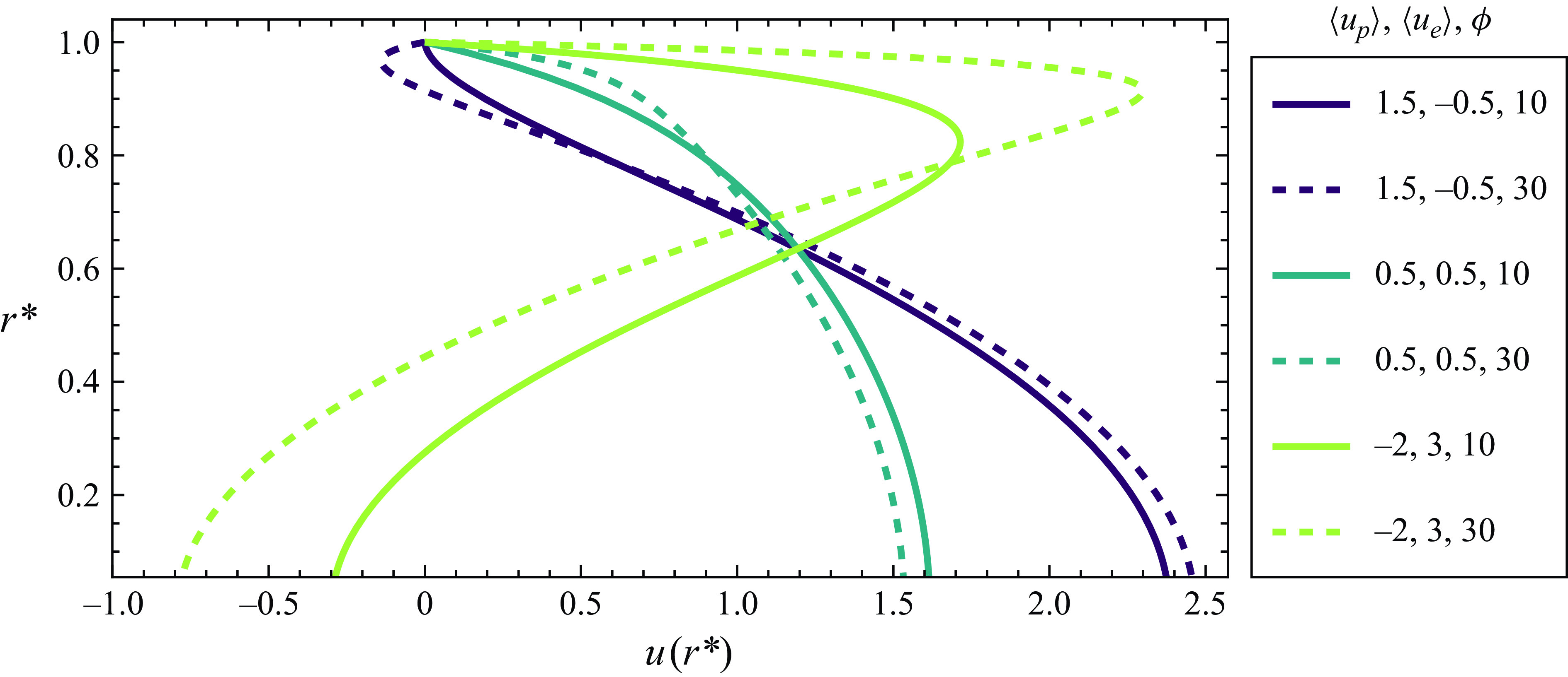
Figure 2 shows examples of the well-known axial flow profiles of combined PDF and EOF in coordinates of $u(r^{*})$
versus the dimensionless inner radius,
$u(r^{*})$
versus the dimensionless inner radius, $r^{*}$
. We show velocity profiles for three combinations of
$r^{*}$
. We show velocity profiles for three combinations of $\langle u_{p}\rangle$
and
$\langle u_{p}\rangle$
and $\langle u_{e}\rangle$
(three line colours) such that
$\langle u_{e}\rangle$
(three line colours) such that $\langle u_{e}\rangle +\langle u_{p}\rangle =1$
. For each combination of
$\langle u_{e}\rangle +\langle u_{p}\rangle =1$
. For each combination of $\langle u_{p}\rangle$
and
$\langle u_{p}\rangle$
and $\langle u_{e}\rangle$
, we present profiles for
$\langle u_{e}\rangle$
, we present profiles for $\phi$
values of 10 and 30 (different line types). We shall later show and discuss EOF profiles where
$\phi$
values of 10 and 30 (different line types). We shall later show and discuss EOF profiles where $\langle u_{p}\rangle \lt 0\lt \langle u_{e}\rangle$
which are useful for minimising the variance of the solute zone. That is, PDF in opposition to bulk EOF can be used to reduce dispersion for a fixed value of overall bulk velocity.
$\langle u_{p}\rangle \lt 0\lt \langle u_{e}\rangle$
which are useful for minimising the variance of the solute zone. That is, PDF in opposition to bulk EOF can be used to reduce dispersion for a fixed value of overall bulk velocity.
Example axial flow profiles for three combinations of PDF and EOF, and two values of the tube radius scaled by the Debye length, $\phi$
. The ordinate shows dimensionless radius,
$\phi$
. The ordinate shows dimensionless radius, $r^{*}$
, and the abscissa is the flow velocity,
$r^{*}$
, and the abscissa is the flow velocity, $u(r^{*})$
. The three line colours correspond to cases of EOF in opposition to bulk PDF, EOF and PDF in the same direction and PDF in opposition to bulk EOF. For each combination of EOF and PDF, profiles are shown for
$u(r^{*})$
. The three line colours correspond to cases of EOF in opposition to bulk PDF, EOF and PDF in the same direction and PDF in opposition to bulk EOF. For each combination of EOF and PDF, profiles are shown for $\phi$
values of 10 and 30 (different line types). All curves were produced with unit bulk velocity.
$\phi$
values of 10 and 30 (different line types). All curves were produced with unit bulk velocity.
2.2. Convective diffusion of solute
We will consider the advective diffusion of a neutral solute subject to the aforementioned velocity profiles. The governing equation, boundary conditions and initial condition for the concentration $c(r,x,t)$
of a solute are
$c(r,x,t)$
of a solute are
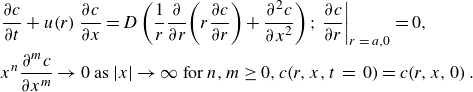 \begin{align} &\frac{\partial c}{\partial t}+u\!\left(r\right)\frac{\partial c}{\partial x}=D\left(\frac{1}{r}\frac{\partial }{\partial r}\!\left(r\frac{\partial c}{\partial r}\right)+\frac{\partial ^{2}c}{\partial x^{2}}\right); \left.\frac{\partial c}{\partial r}\right| _{r\,=\,a,0}=0,\nonumber\\ &x^{n}\frac{\partial ^{m}c}{\partial x^{m}}\rightarrow 0\text{ as }\!\left| x\right| \rightarrow \infty \text{ for }n, m\geq 0,c\!\left(r,x,t\,=\,0\right) = c\!\left(r,x,0\right). \end{align}
Here, the boundary condition at $r=0$
is a result of the assumed azimuthal symmetry and
$r=0$
is a result of the assumed azimuthal symmetry and $c(r,x,0)$
denotes the initial solute distribution. We shall consider two analytical solution methods for this equation in §§ 3 and 4.
$c(r,x,0)$
denotes the initial solute distribution. We shall consider two analytical solution methods for this equation in §§ 3 and 4.
2.3. Brownian dynamics simulations
We will employ Brownian dynamics simulations (Schlick Reference Schlick2002) to benchmark our analytical solutions of the concentration field, effective dispersion coefficient, radial solute distribution and optimal relative magnitudes of EOF and PDF to minimise dispersion. Each of our Brownian dynamics simulations consisted of 5000 point particles. We considered particles distributed initially uniformly across the cross-section of the tube. At each time step in these simulations, each particle is subject to an advection as per (2.4) and a diffusion (random) displacement. The system was allowed to evolve according to the first-order forward Euler method. For each test case, multiple simulations with random seed initial conditions were run, and the reported results represent their average. In this work, we use an identical Brownian dynamics simulation model to that of Chang & Santiago (Reference Chang and Santiago2023) (except for the fact that we here use finer time steps and consider only a channel of uniform radius). This provides a benchmark for the accuracy of our simulations. Additionally, further details around the Brownian dynamics simulations may be found in Chang & Santiago (Reference Chang and Santiago2023). Lastly, all simulation code and results required to recreate the figures of this manuscript may be found on GitHub (csamuel133/Taylor_dispersion_EOF_PDF_Alltime).
3. Taylor dispersion solution of the quasi-steady regime
We here present a derivation of the effective Taylor dispersion (Taylor Reference Taylor1953) for combined PDF and EOF. We will use an area-averaging and deviation formulation (and notation) similar to that of Stone & Brenner (Reference Stone and Brenner1999). Accordingly, we seek to derive the two-dimensional solute concentration field in regimes where the observation time scale is large with respect to the characteristic time of transverse diffusion, for flows described in § 2.1. We expand the concentration and flow fields into cross-sectional averages, defined as $\langle (.)\rangle = (1/\pi a^{2})\int _{0}^{a}2\pi r(.)\mathrm{d}r$
, and deviations therefrom,
$\langle (.)\rangle = (1/\pi a^{2})\int _{0}^{a}2\pi r(.)\mathrm{d}r$
, and deviations therefrom, $(.)^{\prime}$
, such that
$(.)^{\prime}$
, such that $(.)^{\prime} = (.)-\langle (.)\rangle$
. First, we expand (2.6) as
$(.)^{\prime} = (.)-\langle (.)\rangle$
. First, we expand (2.6) as
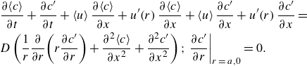 \begin{align} &\frac{\partial \!\left\langle c\right\rangle }{\partial t}+\frac{\partial c^{\prime}}{\partial t}+\left\langle u\right\rangle \frac{\partial \!\left\langle c\right\rangle }{\partial x}+u^{\prime}\!\left(r\right)\frac{\partial \!\left\langle c\right\rangle }{\partial x}+\left\langle u\right\rangle \frac{\partial c^{\prime}}{\partial x}+u^{\prime}\!\left(r\right)\frac{\partial c^{\prime}}{\partial x}=\nonumber\\ &D\left(\frac{1}{r}\frac{\partial }{\partial r}\!\left(r\frac{\partial c^{\prime}}{\partial r}\right)+\frac{\partial ^{2}\!\left\langle c\right\rangle }{\partial x^{2}}+\frac{\partial ^{2}c^{\prime}}{\partial x^{2}}\right);\left.\frac{\partial c^{\prime}}{\partial r}\right| _{r\, =\, a,0}=0. \end{align}
Taking the area average of this equation
 \begin{equation} \frac{\partial \!\left\langle c\right\rangle }{\partial t}+\left\langle u\right\rangle \frac{\partial \!\left\langle c\right\rangle }{\partial x}=D\left(\frac{\partial ^{2}\!\left\langle c\right\rangle }{\partial x^{2}}\right)-\left\langle u^{\prime}\!\left(r\right)\frac{\partial c^{\prime}}{\partial x}\right\rangle .\end{equation}
Subtracting (3.2) from (3.1), we derive an expression for the deviation variable $c^{\prime}$
 \begin{equation} \frac{\partial c^{\prime}}{\partial t}+u^{\prime}\!\left(r\right)\frac{\partial \!\left\langle c\right\rangle }{\partial x}+\left\langle u\right\rangle \frac{\partial c^{\prime}}{\partial x}+u^{\prime}\!\left(r\right)\frac{\partial c^{\prime}}{\partial x}=D\left(\frac{1}{r}\frac{\partial }{\partial r}\!\left(r\frac{\partial c^{\prime}}{\partial r}\right)+\frac{\partial ^{2}c^{\prime}}{\partial x^{2}}\right)+\left\langle u^{\prime}\!\left(r\right)\frac{\partial c^{\prime}}{\partial x}\right\rangle .\end{equation}
The latter equation is again subject to the condition that $\partial c^{\prime}/\partial r| _{r=a,0}=0$
. Let
$\partial c^{\prime}/\partial r| _{r=a,0}=0$
. Let $c_{o}$
denote the characteristic scale (magnitude) of the area-averaged concentration of solute and
$c_{o}$
denote the characteristic scale (magnitude) of the area-averaged concentration of solute and $c_{o}{}^{\prime}$
denote the (much smaller) characteristic scale for the deviation from this average. We non-dimensionalise (3.3) using
$c_{o}{}^{\prime}$
denote the (much smaller) characteristic scale for the deviation from this average. We non-dimensionalise (3.3) using
 \begin{equation} r^{*}=\frac{r}{a} ;\, x_{\sigma^{*}}=\frac{x}{\sigma _{x}} ;\, t^{*}=\frac{t\!\left\langle u\right\rangle }{\sigma _{x}} ;\, {\hat u^{\prime}}=\frac{u^{\prime}\!\left(r\right)}{\left\langle u\right\rangle } ;\, {\left\langle \hat u\right\rangle }=\frac{\left\langle u\right\rangle }{\left\langle u\right\rangle } ;\, c^{\prime*}=\frac{c^{\prime}}{c_{o}{}^{\prime}} ;\, \left\langle c\right\rangle ^{*}=\frac{\left\langle c\right\rangle }{c_{o}} .\end{equation}
Note that we choose the width of the solute cloud as the characteristic axial scale. This choice is different than that of Taylor (Reference Taylor1953) and Stone & Brenner (Reference Stone and Brenner1999), who chose a macroscopic, dimensional length $L$
along the channel to a detector. This is an important distinction as combined (and opposed) PDF and EOF profiles with zero area-averaged net (bulk) velocity result in a dynamic condition wherein the solute zone disperses but its centroid does not move. In the latter case, a distance to a detector L has no meaning. As in Taylor’s (Reference Taylor1953) original analysis, we assume that the magnitude of the area-averaged concentration field is much larger than the magnitude of the deviation therefrom. Next, we assume that the characteristic axial width of the solute cloud is much greater than the inner radius of the tube (
$L$
along the channel to a detector. This is an important distinction as combined (and opposed) PDF and EOF profiles with zero area-averaged net (bulk) velocity result in a dynamic condition wherein the solute zone disperses but its centroid does not move. In the latter case, a distance to a detector L has no meaning. As in Taylor’s (Reference Taylor1953) original analysis, we assume that the magnitude of the area-averaged concentration field is much larger than the magnitude of the deviation therefrom. Next, we assume that the characteristic axial width of the solute cloud is much greater than the inner radius of the tube ( $\sigma _{x}\gg a$
). Further assuming the characteristic advection time of the cloud over
$\sigma _{x}\gg a$
). Further assuming the characteristic advection time of the cloud over $\sigma _{x}$
is large compared with radial diffusion time, we consider three smallness parameters as follows:
$\sigma _{x}$
is large compared with radial diffusion time, we consider three smallness parameters as follows:
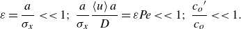 \begin{equation} \varepsilon =\frac{a}{\sigma _{x}}\lt \lt 1 ;\, \frac{a}{\sigma _{x}}\frac{\left\langle u\right\rangle a}{D}=\varepsilon \textit{Pe}\lt \lt 1 ;\, \frac{c_{o}{}^{\prime}}{c_{o}}\lt \lt 1 .\end{equation}
Here, $\textit{Pe}=a\langle u\rangle /D$
is the flow Péclet number. Our non-dimensionalisation of (3.3) then becomes
$\textit{Pe}=a\langle u\rangle /D$
is the flow Péclet number. Our non-dimensionalisation of (3.3) then becomes
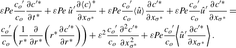 \begin{align} &\varepsilon \textit{Pe}\frac{c_{o}{}^{\prime}}{c_{o}}\frac{\partial c^{\prime*}}{\partial t^{*}}+\varepsilon \textit{Pe} \,{\hat u^{\prime}}\frac{\partial \!\left\langle c\right\rangle^{*}}{\partial x_{\sigma ^{\ast}}}+\varepsilon \textit{Pe}\frac{c_{o}{}^{\prime}}{c_{o}}{\langle \hat u\rangle }\frac{\partial c^{\prime*}}{\partial x_{\sigma^{\ast}}}+\varepsilon \textit{Pe}\frac{c_{o}{}^{\prime}}{c_{o}}{\hat u^{\prime}}\frac{\partial c^{\prime*}}{\partial x_{\sigma^{\ast}}}=\nonumber\\ &\frac{c_{o}{}^{\prime}}{c_{o}}\!\left(\frac{1}{r^{*}}\frac{\partial }{\partial r^{*}}\!\left(r^{*}\frac{\partial c^{\prime*}}{\partial r^{*}}\right)\right)+\varepsilon ^{2}\frac{c_{o}{}^{\prime}}{c_{o}}\frac{\partial ^{2}c^{\prime*}}{\partial x_{\sigma^{\ast}}^{2}}+\varepsilon \textit{Pe}\frac{c_{o}{}^{\prime}}{c_{o}}\!\left\langle {\hat u^{\prime}}\frac{\partial c^{\prime*}}{\partial x_{\sigma ^{\ast}}}\right\rangle . \end{align}
Keeping only terms with one smallness parameter, and keeping only the radial term in dimensionless form, we find
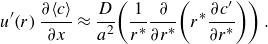 \begin{equation} u^{\prime}\!\left(r\right)\frac{\partial \!\left\langle c\right\rangle }{\partial x}\approx \frac{D}{a^{2}}\!\left(\frac{1}{r^{*}}\frac{\partial }{\partial r^{*}}\!\left(r^{*}\frac{\partial c^{\prime}}{\partial r^{*}}\right)\right) .\end{equation}
This approximate balance between the non-uniform advective dispersion and the radial diffusion is a classic result for Taylor dispersion (Taylor Reference Taylor1953). Next, we multiply (3.7) by $r^{*}$
and integrate,
$r^{*}$
and integrate,
 \begin{align} &\frac{\partial \!\left\langle c\right\rangle }{\partial x}\int \left[r^{*}\!\left(\langle u_{p}\rangle \!\left(1-2r^{*2}\right)+\frac{\left\langle u_{e}\right\rangle }{1-\eta }\!\left(\eta -\frac{I_{0}\!\left(\phi r^{*}\right)}{I_{0}\!\left(\phi \right)}\right)\right)\right]\mathrm{d}r^{*}= \nonumber \\&\quad\frac{\partial \!\left\langle c\right\rangle }{\partial x}\!\left(\langle u_{p} \rangle \!\left(\frac{r^{*2}}{2}-\frac{r^{*4}}{2}\right) +\frac{\left\langle u_{e}\right\rangle }{1-\eta }\!\left(\eta \frac{r^{*2}}{2}-r^{*}\frac{I_{1}\!\left(\phi r^{*}\right)}{\phi I_{0}\!\left(\phi \right)}\right)\right)\approx \frac{D}{a^{2}}\!\left(r^{*}\frac{\partial c^{\prime}}{\partial r^{*}}\right)+C. \end{align}
We use the boundary condition at $r^{*}=1$
to see that the constant of integration
$r^{*}=1$
to see that the constant of integration $C$
must vanish. We divide by
$C$
must vanish. We divide by $r^{*}$
, multiply both sides by
$r^{*}$
, multiply both sides by $a^{2}/D$
, and integrate from 0 to
$a^{2}/D$
, and integrate from 0 to $r^{*}$
, arriving at
$r^{*}$
, arriving at
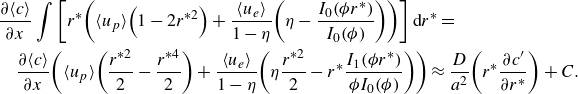
 \begin{align} c^{\prime}\!\left(r,x,t\right)&=c^{\prime}\!\left(0,x,t\right)+\frac{a^{2}}{D}\frac{\partial \!\left\langle c\right\rangle }{\partial x}\!\left(\frac{ \langle u_{p}\rangle }{4}\!\left(r^{*2}-\frac{r^{*4}}{2}\right)\right.\nonumber \\&\quad+\left.\frac{\left\langle u_{e}\right\rangle }{1-\eta }\!\left(\eta \frac{r^{*2}}{4}-\frac{I_{0}\!\left(\phi r^{*}\right)-1}{\phi ^{2}I_{0}\!\left(\phi \right)}\right)\right). \end{align}
Applying cross-sectional averaging, we are left with
 \begin{equation} 0=c^{\prime}\!\left(0,x,t\right)+\frac{a^{2}}{D}\frac{\partial \!\left\langle c\right\rangle }{\partial x}\!\left(\frac{ \langle u_{p} \rangle }{12}+\frac{\left\langle u_{e}\right\rangle }{1-\eta }\!\left(\frac{\eta }{8}-\frac{\eta }{\phi ^{2}}+\frac{1}{\phi ^{2}I_{0}\!\left(\phi \right)}\right)\right) .\end{equation}
Subtracting (3.10) from (3.9), we derive
 \begin{align} c^{\prime}\!\left(r,x,t\right)&=\frac{a^{2}}{D}\frac{\partial \!\left\langle c\right\rangle }{\partial x}\!\left(\frac{ \langle u_{p} \rangle }{4}\!\left(r^{*2}-\frac{1}{3}-\frac{r^{*4}}{2}\right)\right.\nonumber \\&\quad+\left.\frac{\left\langle u_{e}\right\rangle }{1-\eta }\!\left(-\frac{\eta }{8}+\frac{\eta }{\phi ^{2}}+\eta \frac{r^{*2}}{4}-\frac{I_{0}\!\left(\phi r^{*}\right)}{\phi ^{2}I_{0}\!\left(\phi \right)}\right)\right) . \end{align}
Equation (3.11), combined with our solution for $\partial \langle c\rangle /\partial x$
, will provide an analytical expression for the unsteady, two-dimensional (radial and axial) distribution of the solute. To our knowledge, this is the first reported expression for the radial concentration of solute for combined EOF and PDF. We will use (3.11) to show solute concentration profiles versus axial position for several values of
$\partial \langle c\rangle /\partial x$
, will provide an analytical expression for the unsteady, two-dimensional (radial and axial) distribution of the solute. To our knowledge, this is the first reported expression for the radial concentration of solute for combined EOF and PDF. We will use (3.11) to show solute concentration profiles versus axial position for several values of $r^{*}$
in figure 3. We will then visualise the two-dimensional solute concentration field in figures 4 and 5, and visualise the radial solute distribution alone in figure 6. Returning to (3.9), we take the derivative with respect to
$r^{*}$
in figure 3. We will then visualise the two-dimensional solute concentration field in figures 4 and 5, and visualise the radial solute distribution alone in figure 6. Returning to (3.9), we take the derivative with respect to $x$
, multiply by
$x$
, multiply by $u^{\prime}(r)$
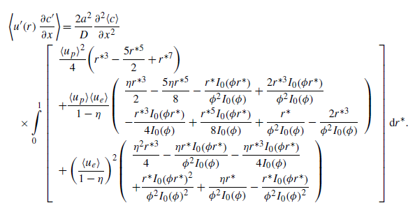
, and apply cross-sectional averaging
$u^{\prime}(r)$
, and apply cross-sectional averaging
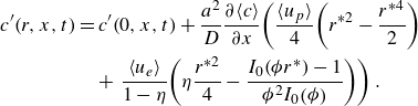
The four figure panels show axial solute concentration profiles corresponding to four combinations of the Péclet number based on EOF, $\textit{Pe}_{e}$
, the Péclet number based on PDF,
$\textit{Pe}_{e}$
, the Péclet number based on PDF, $\textit{Pe}_{p}$
, and the tube radius scaled by Debye length,
$\textit{Pe}_{p}$
, and the tube radius scaled by Debye length, $\phi$
. The ordinate shows dimensionless solute concentration,
$\phi$
. The ordinate shows dimensionless solute concentration, $c^{*}(x^{\prime*}|r^{*},\tau )=\pi a^{3}c(x^{\prime*}|r^{*},\tau )/N$
, and the abscissa is dimensionless axial position in a frame moving at the solute bulk velocity,
$c^{*}(x^{\prime*}|r^{*},\tau )=\pi a^{3}c(x^{\prime*}|r^{*},\tau )/N$
, and the abscissa is dimensionless axial position in a frame moving at the solute bulk velocity, $x^{\prime*}=x^{*}-\tau P\hspace{0pt}e$
. In each panel, solute concentration curves are shown at three values of dimensionless time (different line colours) for three distinct dimensionless radial positions (different line types), resulting in nine total concentration profiles per panel. The dimensionless solute concentration is obtained by evaluating (3.40) for an initial ‘top hat’ of solute with a width negligible to the final axial width of the solute and then normalising the solute concentration as
$x^{\prime*}=x^{*}-\tau P\hspace{0pt}e$
. In each panel, solute concentration curves are shown at three values of dimensionless time (different line colours) for three distinct dimensionless radial positions (different line types), resulting in nine total concentration profiles per panel. The dimensionless solute concentration is obtained by evaluating (3.40) for an initial ‘top hat’ of solute with a width negligible to the final axial width of the solute and then normalising the solute concentration as $c^{*}(x^{\prime*}|r^{*},\tau )=\pi a^{3}c(x^{\prime*}|r^{*},\tau )/N$
.
$c^{*}(x^{\prime*}|r^{*},\tau )=\pi a^{3}c(x^{\prime*}|r^{*},\tau )/N$
.
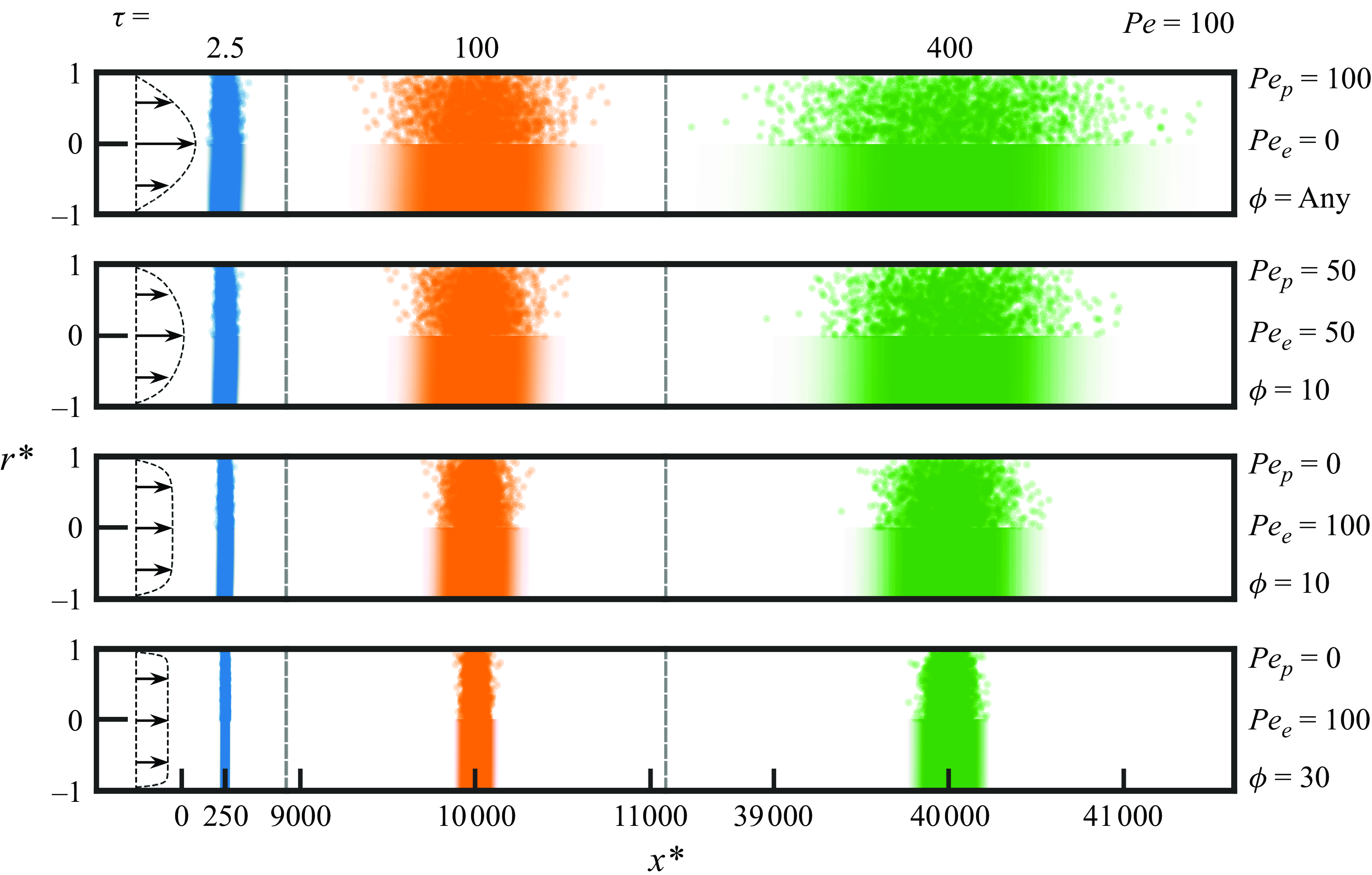
Benchmark comparisons between Brownian dynamics simulations and the analytical solution of the quasi-steady solute concentration field at three values of dimensionless time, $\tau =\textit{tD}/a^{2}$
. The figure shows dimensionless radius,
$\tau =\textit{tD}/a^{2}$
. The figure shows dimensionless radius, $r^{*}$
, on the ordinate and dimensionless axial position,
$r^{*}$
, on the ordinate and dimensionless axial position, $x^{*}$
, on the abscissa. The top half of each panel shows individual particles from the Brownian dynamics simulations and the bottom half of each panel shows the concentration field predicted by the analytical solution in (3.40). Panels show four combinations of the Péclet number based on PDF,
$x^{*}$
, on the abscissa. The top half of each panel shows individual particles from the Brownian dynamics simulations and the bottom half of each panel shows the concentration field predicted by the analytical solution in (3.40). Panels show four combinations of the Péclet number based on PDF, $P\hspace{0pt}e_{p}$
, the Péclet number based on EOF,
$P\hspace{0pt}e_{p}$
, the Péclet number based on EOF, $P\hspace{0pt}e_{e}$
, and the tube radius scaled by Debye length,
$P\hspace{0pt}e_{e}$
, and the tube radius scaled by Debye length, $\phi$
. The far left of the panels shows the flow profile used to generate the data for each row. Figure was produced with a Péclet number of
$\phi$
. The far left of the panels shows the flow profile used to generate the data for each row. Figure was produced with a Péclet number of $\textit{Pe}=100$
(§ B of the SM has similar figures for
$\textit{Pe}=100$
(§ B of the SM has similar figures for $\textit{Pe}=$
20 and 1000).
$\textit{Pe}=$
20 and 1000).
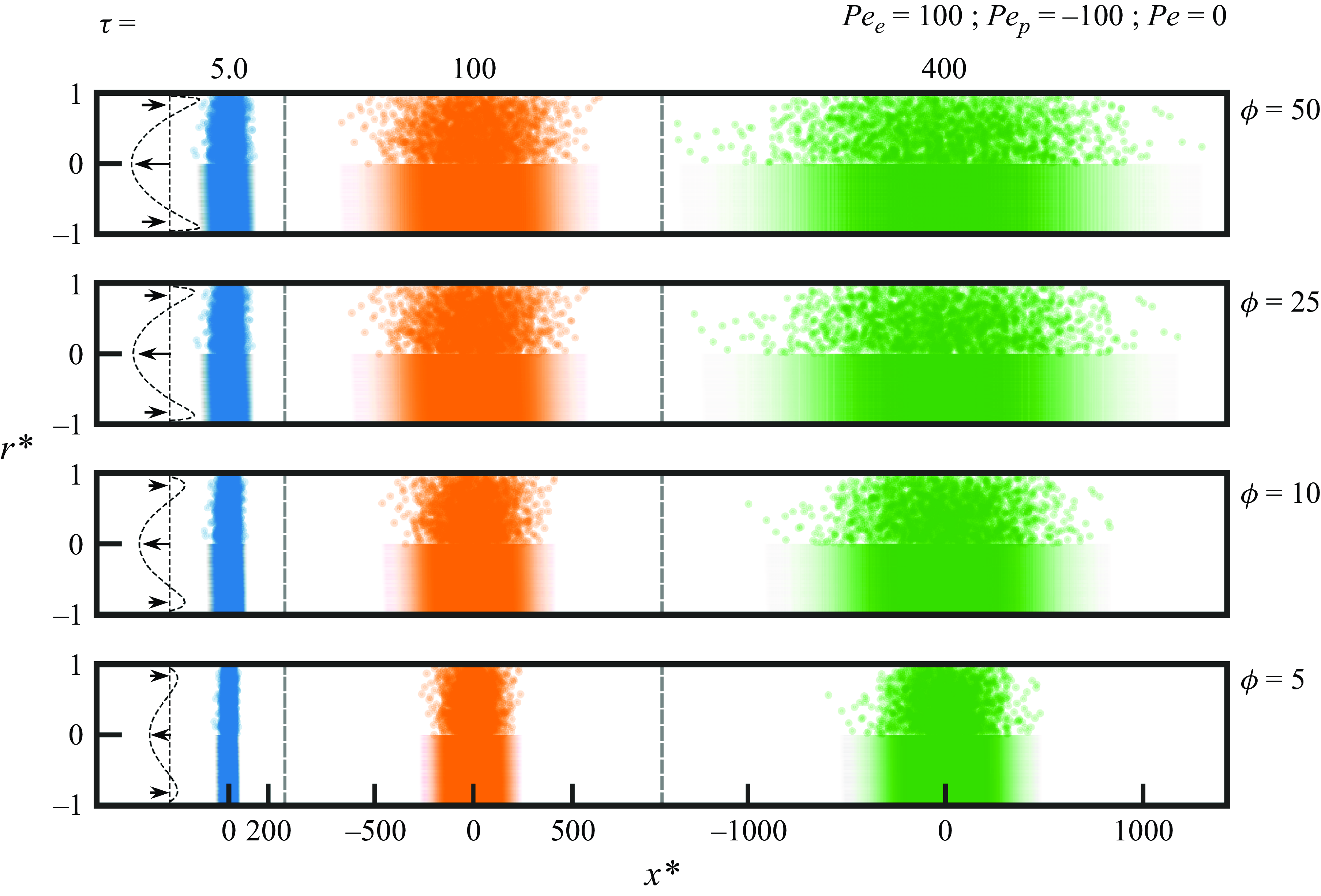
Benchmark comparisons between Brownian dynamics simulations and the analytical solution of the quasi-steady solute concentration field at three values of dimensionless time, $\tau =\textit{tD}/a^{2}$
. Solute zones were subject to flows wherein EOF is perfectly opposed by PDF to achieve a net flow with zero area-averaged bulk velocity. Panels show solute zones for four values of the tube radius scaled by Debye length,
$\tau =\textit{tD}/a^{2}$
. Solute zones were subject to flows wherein EOF is perfectly opposed by PDF to achieve a net flow with zero area-averaged bulk velocity. Panels show solute zones for four values of the tube radius scaled by Debye length, $\phi$
. The figure shows dimensionless radius,
$\phi$
. The figure shows dimensionless radius, $r^{*}$
, on the ordinate and dimensionless axial position,
$r^{*}$
, on the ordinate and dimensionless axial position, $x^{*}$
, on the abscissa. The top half of each panel shows individual particles from the Brownian dynamics simulations and the bottom half of each panel shows the concentration field predicted by the analytical solution in (3.40). The far left of the panels shows the flow profile used to generate the data for each row. Figure was produced with Péclet numbers based on EOF bulk velocity and PDF bulk velocity of
$x^{*}$
, on the abscissa. The top half of each panel shows individual particles from the Brownian dynamics simulations and the bottom half of each panel shows the concentration field predicted by the analytical solution in (3.40). The far left of the panels shows the flow profile used to generate the data for each row. Figure was produced with Péclet numbers based on EOF bulk velocity and PDF bulk velocity of $\textit{Pe}_{e}=100$
and
$\textit{Pe}_{e}=100$
and $\textit{Pe}_{p}=-100$
, respectively.
$\textit{Pe}_{p}=-100$
, respectively.
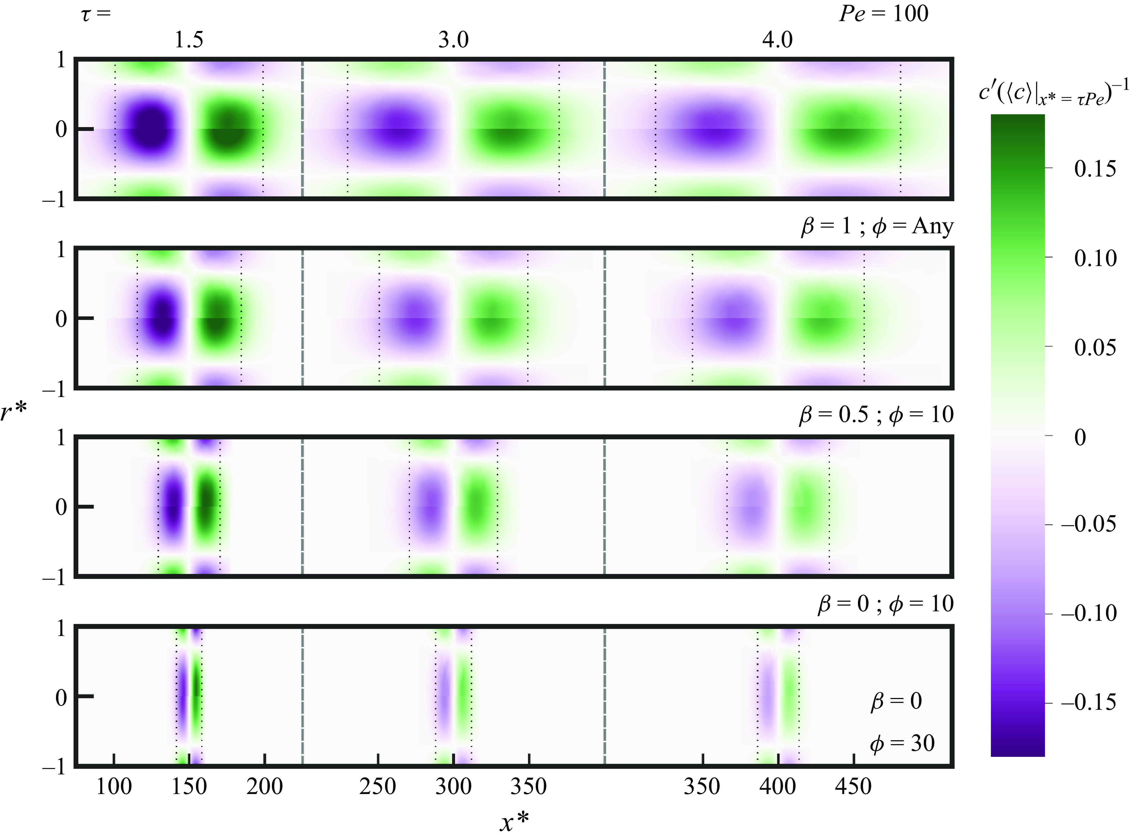
Comparisons between the analytical solution and Brownian dynamics simulations of the normalised quasi-steady radial distribution of solute at three values of dimensionless time, $\tau$
. The radial distribution is normalised as
$\tau$
. The radial distribution is normalised as $c^{\prime}(r^{*},x^{*},\tau )/\langle c\rangle (x^{*}=\tau \textit{Pe},\tau )$
where
$c^{\prime}(r^{*},x^{*},\tau )/\langle c\rangle (x^{*}=\tau \textit{Pe},\tau )$
where $\langle c\rangle (x^{*}=\tau \textit{Pe},\tau )$
is the area-averaged concentration at the mean axial position of solute. Dimensionless radius,
$\langle c\rangle (x^{*}=\tau \textit{Pe},\tau )$
is the area-averaged concentration at the mean axial position of solute. Dimensionless radius, $r^{*}$
, is shown on the ordinate and dimensionless axial position,
$r^{*}$
, is shown on the ordinate and dimensionless axial position, $x^{*}$
, is shown on the abscissa. The top half of each panel shows the radial solute distribution calculated from the Brownian dynamics simulations and the bottom half of each panel shows the analytical solution (given by the second term on the right-hand side of (3.40)). Panels show four combinations of the fraction of bulk velocity caused by pressure,
$x^{*}$
, is shown on the abscissa. The top half of each panel shows the radial solute distribution calculated from the Brownian dynamics simulations and the bottom half of each panel shows the analytical solution (given by the second term on the right-hand side of (3.40)). Panels show four combinations of the fraction of bulk velocity caused by pressure, $\beta$
, and the tube radius scaled by Debye length,
$\beta$
, and the tube radius scaled by Debye length, $\phi$
. The dotted black lines denote two axial standard deviations of the Brownian particles’ position about their mean position. Figure was produced with a Péclet number of
$\phi$
. The dotted black lines denote two axial standard deviations of the Brownian particles’ position about their mean position. Figure was produced with a Péclet number of $\textit{Pe}=100$
.
$\textit{Pe}=100$
.
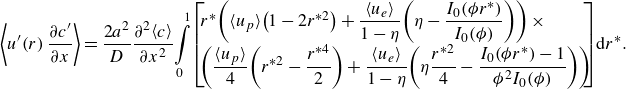 \begin{equation} \left\langle u^{\prime}\!\left(r\right)\frac{\partial c^{\prime}}{\partial x}\right\rangle =\frac{2a^{2}}{D}\frac{\partial ^{2}\!\left\langle c\right\rangle }{\partial x^{2}}\!\int \limits_{0}^{1}\!\left[\!\!\begin{array}{l} r^{*}\!\left( \langle u_{p} \rangle \!\left(1-2r^{*2}\right)+\dfrac{\left\langle u_{e}\right\rangle }{1-\eta }\!\left(\eta -\dfrac{I_{0}\!\left(\phi r^{*}\right)}{I_{0}\!\left(\phi \right)}\right)\right) \times \\[6pt]\left(\dfrac{ \langle u_{p} \rangle }{4}\!\left(r^{*2}-\dfrac{r^{*4}}{2}\right)+\dfrac{\left\langle u_{e}\right\rangle }{1-\eta }\!\left(\eta \dfrac{r^{*2}}{4}-\dfrac{I_{0}\!\left(\phi r^{*}\right)-1}{\phi ^{2}I_{0}\!\left(\phi \right)}\right)\right) \end{array}\!\!\!\right]\!\mathrm{d}r^{*}. \end{equation}
Expanding the right-hand side of (3.12) and simplifying yields 17 terms. We collect these into three groups as follows:
 \begin{align} &\left\langle u^{\prime}\!\left(r\right)\dfrac{\partial c^{\prime}}{\partial x}\right\rangle =\dfrac{2a^{2}}{D}\dfrac{\partial ^{2}\!\left\langle c\right\rangle }{\partial x^{2}}\nonumber\\&\quad \times \int \limits_{0}^{1} \left[\begin{array}{l} \dfrac{ \langle u_{p} \rangle ^{2}}{4}\!\left(r^{*3}-\dfrac{5r^{*5}}{2}+r^{*7}\right)\\[9pt] +\dfrac{ \langle u_{p} \rangle \!\left\langle u_{e}\right\rangle }{1-\eta }\!\left(\begin{array}{l} \dfrac{\eta r^{*3}}{2}-\dfrac{5\eta r^{*5}}{8}-\dfrac{r^{*}I_{0}\!\left(\phi r^{*}\right)}{\phi ^{2}I_{0}\!\left(\phi \right)}+\dfrac{2r^{*3}I_{0}\!\left(\phi r^{*}\right)}{\phi ^{2}I_{0}\!\left(\phi \right)}\\[9pt] -\dfrac{r^{*3}I_{0}\!\left(\phi r^{*}\right)}{4I_{0}\!\left(\phi \right)}+\dfrac{r^{*5}I_{0}\!\left(\phi r^{*}\right)}{8I_{0}\!\left(\phi \right)}+\dfrac{r^{*}}{\phi ^{2}I_{0}\!\left(\phi \right)}-\dfrac{2r^{*3}}{\phi ^{2}I_{0}\!\left(\phi \right)} \end{array}\right)\\[26pt] +\left(\dfrac{\left\langle u_{e}\right\rangle }{1-\eta }\right)^{2}\!\left(\begin{array}{l} \dfrac{\eta ^{2}r^{*3}}{4}-\dfrac{\eta r^{*}I_{0}\!\left(\phi r^{*}\right)}{\phi ^{2}I_{0}\!\left(\phi \right)}-\dfrac{\eta r^{*3}I_{0}\!\left(\phi r^{*}\right)}{4I_{0}\!\left(\phi \right)}\\[9pt] +\dfrac{r^{*}I_{0}\!\left(\phi r^{*}\right)^{2}}{\phi ^{2}I_{0}\!\left(\phi \right)^{2}}+\dfrac{\eta r^{*}}{\phi ^{2}I_{0}\!\left(\phi \right)}-\dfrac{r^{*}I_{0}\!\left(\phi r^{*}\right)}{\phi ^{2}I_{0}\!\left(\phi \right)^{2}} \end{array}\right) \end{array}\right]\mathrm{d}r^{*} .\nonumber\\[5pt] \end{align}
Evaluating the integral in (3.13), we obtain
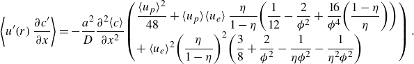 \begin{equation} \left\langle u^{\prime}\!\left(r\right)\dfrac{\partial c^{\prime}}{\partial x}\right\rangle =-\dfrac{a^{2}}{D}\dfrac{\partial ^{2}\!\left\langle c\right\rangle }{\partial x^{2}}\!\left(\begin{array}{l} \dfrac{ \langle u_{p} \rangle ^{2}}{48}+ \langle u_{p} \rangle \!\left\langle u_{e}\right\rangle \dfrac{\eta }{1-\eta }\!\left(\dfrac{1}{12}-\dfrac{2}{\phi ^{2}}+\dfrac{16}{\phi ^{4}}\!\left(\dfrac{1-\eta }{\eta }\right)\right)\\ +\left\langle u_{e}\right\rangle ^{2}\!\left(\dfrac{\eta }{1-\eta }\right)^{2}\!\left(\dfrac{3}{8}+\dfrac{2}{\phi ^{2}}-\dfrac{1}{\eta \phi ^{2}}-\dfrac{1}{\eta ^{2}\phi ^{2}}\right) \end{array}\right) .\end{equation}
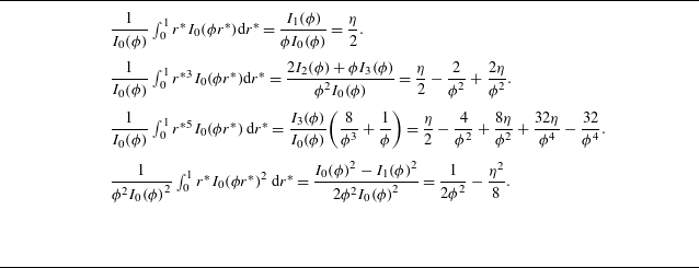
Table 1 lists the relevant integrals involving modified Bessel functions of the first kind which were used in this evaluation. Next, for a compact notation, we define
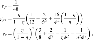 \begin{align} \gamma _{p}&=\frac{1}{48}\nonumber\\ \gamma _{pe}&=\frac{\eta }{1-\eta }\!\left(\frac{1}{12}-\frac{2}{\phi ^{2}}+\frac{16}{\phi ^{4}}\!\left(\frac{1-\eta }{\eta }\right)\right)\nonumber\\ \gamma _{e}&=\left(\frac{\eta }{1-\eta }\right)^{2}\!\left(\frac{3}{8}+\frac{2}{\phi ^{2}}-\frac{1}{\eta \phi ^{2}}-\frac{1}{\eta ^{2}\phi ^{2}}\right), \end{align}
which allows us to express (3.14) as
 \begin{equation} \left\langle u^{\prime}\!\left(r\right)\frac{\partial c^{\prime}}{\partial x}\right\rangle =-\frac{a^{2}}{D}\frac{\partial ^{2}\!\left\langle c\right\rangle }{\partial x^{2}}\!\left( \langle u_{p} \rangle ^{2}\gamma _{p}+ \langle u_{p}\rangle \!\left\langle u_{e}\right\rangle \gamma _{pe}+\left\langle u_{e}\right\rangle ^{2}\gamma _{e}\right) .\end{equation}
Substituting (3.16) into (3.2), we derive the following one-dimensional, unsteady partial differential equation describing the area-averaged concentration field:
 \begin{equation} \frac{\partial \!\left\langle c\right\rangle }{\partial t}+\left\langle u\right\rangle \frac{\partial \!\left\langle c\right\rangle }{\partial x}=\frac{\partial ^{2}\!\left\langle c\right\rangle }{\partial x^{2}}\!\left(D+\frac{a^{2}}{D}\!\left( \langle u_{p}\rangle ^{2}\gamma _{p}+ \langle u_{p} \rangle \!\left\langle u_{e}\right\rangle \gamma _{pe}+\left\langle u_{e}\right\rangle ^{2}\gamma _{e}\right)\right) .\end{equation}
Integrals applicable to the evaluation of (3.13).
The first, third and second parenthetic terms on the right-hand side respectively capture the effects of dispersion caused by PDF alone, by EOF alone and by the coupled, non-superposable effects of simultaneous PDF and EOF. From the latter equation, the effective dispersion coefficient valid for the Taylor-type limit of the problem is
 \begin{equation} D_{\textit{eff}}=D+\frac{a^{2}}{D}\!\left( \langle u_{p} \rangle ^{2}\gamma _{p} + \langle u_{p} \rangle \!\left\langle u_{e}\right\rangle \gamma _{pe}+\left\langle u_{e}\right\rangle ^{2}\gamma _{e}\right) .\end{equation}
Note that, in analogy to Taylor’s (Reference Taylor1953) original analysis, (3.17) has the form of a one-dimensional unsteady diffusion equation with the molecular diffusivity replaced by an effective dispersion coefficient given by (3.18). As such, the solution is an initial value problem that requires an initial axial distribution of the area-averaged solute. However, the solution of (3.17) does not accurately predict the evolution of solute until sufficient time has passed relative to the characteristic time of transverse diffusion, $a^{2}/D$
. In other words, this solution is valid as long as the solute variance gained in early times (during the pre-asymptotic dispersion regime) is small compared with either the initial variance or the variance gained due to the (long-term) Taylor dispersion. We will soon explore predictions by this solution given specific initial conditions. In § 4, we will derive dispersion solutions (given various initial conditions) which are valid for both short and long times. Next, we note that (3.18) is equivalent to the solution reported by Datta & Kotamarthi (Reference Datta and Kotamarthi1990) for the dimensional dispersion coefficient (see their equation (37)). Datta & Kotamarthi reported deriving their solution by applying a Taylor-type analysis but, as mentioned earlier, did not present a derivation in any detail. Further, we note that (3.18), for pure PDF (
$a^{2}/D$
. In other words, this solution is valid as long as the solute variance gained in early times (during the pre-asymptotic dispersion regime) is small compared with either the initial variance or the variance gained due to the (long-term) Taylor dispersion. We will soon explore predictions by this solution given specific initial conditions. In § 4, we will derive dispersion solutions (given various initial conditions) which are valid for both short and long times. Next, we note that (3.18) is equivalent to the solution reported by Datta & Kotamarthi (Reference Datta and Kotamarthi1990) for the dimensional dispersion coefficient (see their equation (37)). Datta & Kotamarthi reported deriving their solution by applying a Taylor-type analysis but, as mentioned earlier, did not present a derivation in any detail. Further, we note that (3.18), for pure PDF ( $\langle u_{p}\rangle =\langle u\rangle$
), reduces to Aris’ (Reference Aris1956) classic solution of
$\langle u_{p}\rangle =\langle u\rangle$
), reduces to Aris’ (Reference Aris1956) classic solution of $D_{\textit{eff}}=D+D^{-1}a^{2}\langle u_{p}\rangle ^{2}\gamma _{p}$
. Additionally, for pure EOF (
$D_{\textit{eff}}=D+D^{-1}a^{2}\langle u_{p}\rangle ^{2}\gamma _{p}$
. Additionally, for pure EOF ( $\langle u_{e}\rangle =\langle u\rangle$
), (3.18) becomes
$\langle u_{e}\rangle =\langle u\rangle$
), (3.18) becomes $D_{\textit{eff}}=D+D^{-1}a^{2}\langle u_{e}\rangle ^{2}\gamma _{e}$
, which agrees analytically with Griffiths & Nilson’s (Reference Griffiths and Nilson1999) solution of the coefficient of effective dispersion (their equation (38); see § A of the supplementary material (SM) for proof).
$D_{\textit{eff}}=D+D^{-1}a^{2}\langle u_{e}\rangle ^{2}\gamma _{e}$
, which agrees analytically with Griffiths & Nilson’s (Reference Griffiths and Nilson1999) solution of the coefficient of effective dispersion (their equation (38); see § A of the supplementary material (SM) for proof).
Next, we scale the expression for the dispersion coefficient. To this end, we note that $\langle u_{p}\rangle$
and
$\langle u_{p}\rangle$
and $\langle u_{e}\rangle$
are signed quantities. They are also variables which are fully independent of each other (e.g. they can be independently controlled in an experiment). Hence, we define here two corresponding (signed) Péclet numbers of the form
$\langle u_{e}\rangle$
are signed quantities. They are also variables which are fully independent of each other (e.g. they can be independently controlled in an experiment). Hence, we define here two corresponding (signed) Péclet numbers of the form $P\hspace{0pt}e_{p}=a\langle u_{p}\rangle /D$
and
$P\hspace{0pt}e_{p}=a\langle u_{p}\rangle /D$
and $P\hspace{0pt}e_{e}=a\langle u_{e}\rangle /D$
. For both, we use the characteristic length scale of the cylinder radius. The non-dimensional dispersion coefficient is then
$P\hspace{0pt}e_{e}=a\langle u_{e}\rangle /D$
. For both, we use the characteristic length scale of the cylinder radius. The non-dimensional dispersion coefficient is then
 \begin{equation} D_{\textit{eff}}^{*}=\frac{D_{\textit{eff}}}{D}=1+\textit{Pe}_{p}^{2}\gamma _{p}+\textit{Pe}_{p}\textit{Pe}_{e} \gamma _{pe}+\textit{Pe}_{e}^{2}\gamma _{e} .\end{equation}
The last three terms on the right-hand side again capture the effects of pure PDF, coupled PDF and EOF and pure EOF. Because the values of $\gamma$
are functions of
$\gamma$
are functions of $\phi$
(cf. (3.15)),
$\phi$
(cf. (3.15)), $D_{\textit{eff}}^{*}$
is a function of only three dimensionless parameters:
$D_{\textit{eff}}^{*}$
is a function of only three dimensionless parameters: $\textit{Pe}_{p}, \textit{Pe}_{e}$
and
$\textit{Pe}_{p}, \textit{Pe}_{e}$
and $\phi$
.
$\phi$
.
Before continuing our presentation, we briefly compare our (3.19) with the non-dimensional dispersion coefficient presented by Datta & Kotamarthi (Reference Datta and Kotamarthi1990). The latter authors chose to combine the signed quantities $\langle u_{p}\rangle$
and
$\langle u_{p}\rangle$
and $\langle u_{e}\rangle$
as a sum within a single global Péclet number of the form
$\langle u_{e}\rangle$
as a sum within a single global Péclet number of the form $\textit{Pe}=(\langle u_{p}\rangle +\langle u_{e}\rangle )a/D$
. Further, they chose to use the ratio
$\textit{Pe}=(\langle u_{p}\rangle +\langle u_{e}\rangle )a/D$
. Further, they chose to use the ratio $\beta =\langle u_{p}\rangle /\langle u\rangle$
to distinguish between the effects of EOF and PDF. Their approach yields the following result:
$\beta =\langle u_{p}\rangle /\langle u\rangle$
to distinguish between the effects of EOF and PDF. Their approach yields the following result:
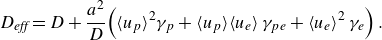
 \begin{equation} D_{\textit{eff}}^{*}=1+P\hspace{0pt}e^{2}\!\left(\beta ^{2}\gamma _{p}+\beta \left(1-\beta \right)\gamma _{pe}+\left(1-\beta \right)^{2}\gamma _{e}\right) .\end{equation}
In this formulation, $D_{\textit{eff}}^{*}$
is again a function of three parameters, but these are now
$D_{\textit{eff}}^{*}$
is again a function of three parameters, but these are now $\phi, \beta$
and
$\phi, \beta$
and $P\hspace{0pt}e$
. We note this combination of two velocity scales into a single Péclet number is most useful to characterise dispersion when EOF and PDF act in the same direction. We recommend the formulation of (3.19) for cases wherein EOF and PDF are in opposition. When EOF and PDF are opposed and nearly equal in magnitude,
$P\hspace{0pt}e$
. We note this combination of two velocity scales into a single Péclet number is most useful to characterise dispersion when EOF and PDF act in the same direction. We recommend the formulation of (3.19) for cases wherein EOF and PDF are in opposition. When EOF and PDF are opposed and nearly equal in magnitude, $P\hspace{0pt}e$
approaches zero while
$P\hspace{0pt}e$
approaches zero while $\beta$
approaches infinity at the same rate and evaluation of (3.20) is more cumbersome than (3.19).
$\beta$
approaches infinity at the same rate and evaluation of (3.20) is more cumbersome than (3.19).
We can rewrite (3.20) as follows:
 \begin{equation} \frac{48}{\textit{Pe}^{2}}\!\left(D_{\textit{eff}}^{*}-1\right)=48\left(\beta ^{2}\gamma _{p}+\beta \!\left(1-\beta \right)\gamma _{pe}+\left(1-\beta \right)^{2}\gamma _{e}\right) .\end{equation}
This formulation enables exploration of the full solution and in a manner most useful when EOF and PDF are not perfectly opposed. We will use this formulation to plot and benchmark the grouping $48\textit{Pe}^{-2}(D_{\textit{eff}}^{*}-1)$
in heatmaps where the independent variables are
$48\textit{Pe}^{-2}(D_{\textit{eff}}^{*}-1)$
in heatmaps where the independent variables are $\beta$
and
$\beta$
and $\phi$
(see figure 7). Further, we will benchmark
$\phi$
(see figure 7). Further, we will benchmark $D_{\textit{eff}}^{*}$
against Brownian dynamics simulations for the case of perfectly opposed PDF and EOF in figure 8. Lastly, we note (3.21) conveniently reduces to unity for the case of parabolic flow. Parabolic flow is achieved by pure PDF or for combinations of PDF and EOF with thick EDLs (since thick-EDL solutions also lead to parabolic EOF).
$D_{\textit{eff}}^{*}$
against Brownian dynamics simulations for the case of perfectly opposed PDF and EOF in figure 8. Lastly, we note (3.21) conveniently reduces to unity for the case of parabolic flow. Parabolic flow is achieved by pure PDF or for combinations of PDF and EOF with thick EDLs (since thick-EDL solutions also lead to parabolic EOF).
Contour plots of our quasi-steady analytical solution $(a)$
versus Brownian dynamics simulations
$(a)$
versus Brownian dynamics simulations $(b)$
of the normalised effective dispersion coefficient. In both cases, the effective dispersion coefficient is normalised as
$(b)$
of the normalised effective dispersion coefficient. In both cases, the effective dispersion coefficient is normalised as $48\textit{Pe}^{-2}(D_{\textit{eff}}^{*}-1)$
where
$48\textit{Pe}^{-2}(D_{\textit{eff}}^{*}-1)$
where $D_{\textit{eff}}^{*}$
is the effective dispersion coefficient. This non-dimensional quantity is plotted versus the fraction of bulk velocity caused by pressure,
$D_{\textit{eff}}^{*}$
is the effective dispersion coefficient. This non-dimensional quantity is plotted versus the fraction of bulk velocity caused by pressure, $\beta$
, and the radius scaled by Debye length,
$\beta$
, and the radius scaled by Debye length, $\phi$
. The panels cover the entire dynamics of quasi-steady dispersion for all relative EDL thicknesses and many velocity profiles. The white dashed lines show the variance-minimising contour for values of
$\phi$
. The panels cover the entire dynamics of quasi-steady dispersion for all relative EDL thicknesses and many velocity profiles. The white dashed lines show the variance-minimising contour for values of $\beta$
as a function of
$\beta$
as a function of $\phi$
. These lines are obtained from (3.32) for the analytical solution and numerically for the Brownian dynamics simulations.
$\phi$
. These lines are obtained from (3.32) for the analytical solution and numerically for the Brownian dynamics simulations.
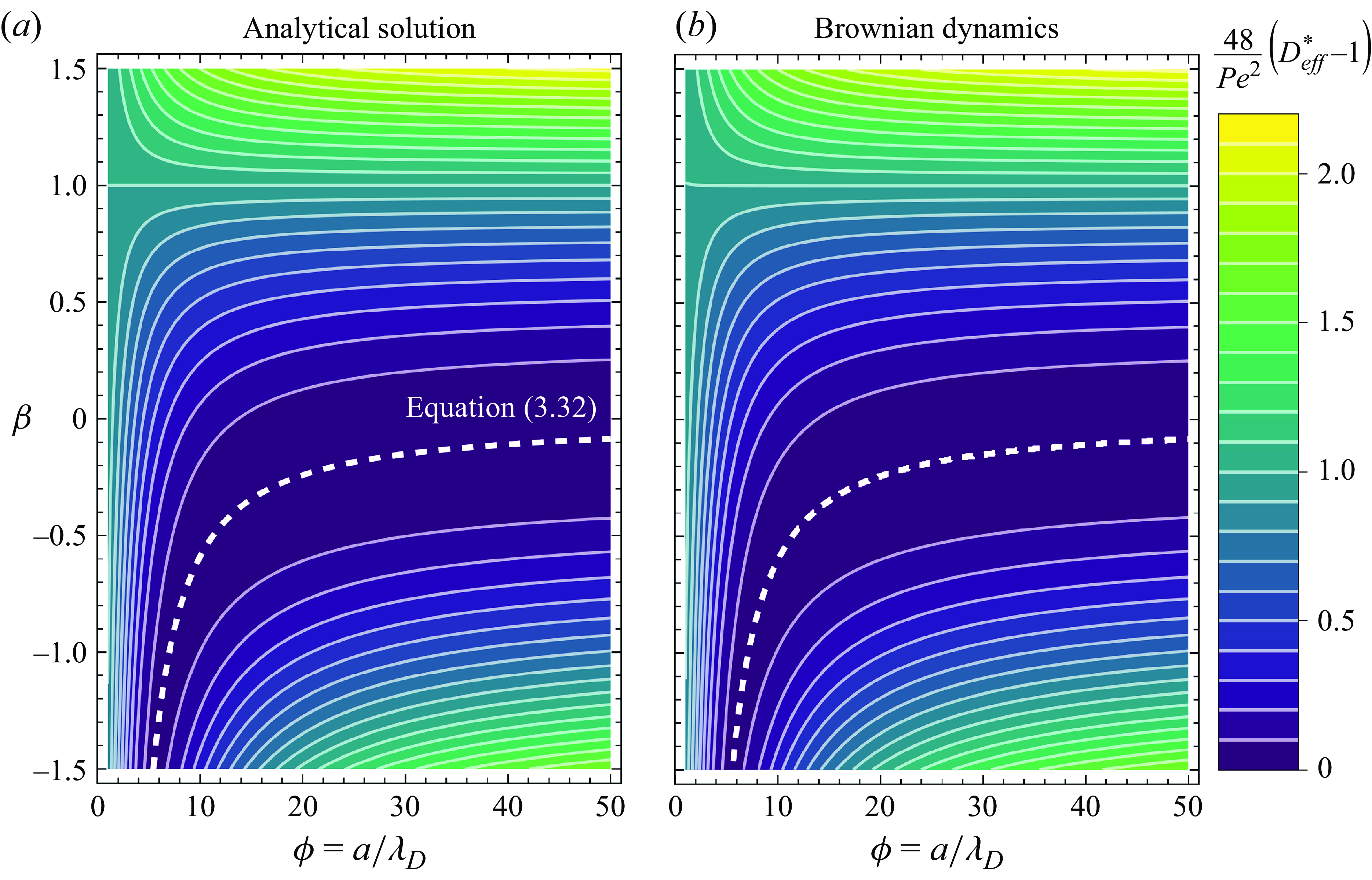
Contour plots of our quasi-steady analytical solution $(a)$
versus Brownian dynamics simulations
$(a)$
versus Brownian dynamics simulations $(b)$
of the dimensionless effective dispersion coefficient for the case of perfectly opposed EOF and PDF. The dimensionless dispersion coefficient
$(b)$
of the dimensionless effective dispersion coefficient for the case of perfectly opposed EOF and PDF. The dimensionless dispersion coefficient $D_{\textit{eff}}^{*}$
is plotted versus the Péclet number based on PDF,
$D_{\textit{eff}}^{*}$
is plotted versus the Péclet number based on PDF, $P\hspace{0pt}e_{p}$
, and the radius scaled by Debye length,
$P\hspace{0pt}e_{p}$
, and the radius scaled by Debye length, $\phi$
. The Péclet number based on PDF is fixed to be equal in magnitude but opposite in sign to the Péclet number based on EOF,
$\phi$
. The Péclet number based on PDF is fixed to be equal in magnitude but opposite in sign to the Péclet number based on EOF, $P\hspace{0pt}e_{e}$
. For perfectly opposed PDF and EOF,
$P\hspace{0pt}e_{e}$
. For perfectly opposed PDF and EOF, $D_{\textit{eff}}^{*}$
decreases as
$D_{\textit{eff}}^{*}$
decreases as $\phi$
decreases.
$\phi$
decreases.
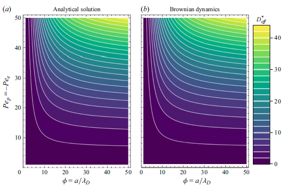
We now continue with our derivation for the two-dimensional concentration field. We first evaluate the solution of (3.17) for an initial delta function condition for the solute of the form
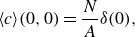 \begin{equation} \left\langle c\right\rangle \!\left(0,0\right)=\frac{N}{A}\delta (0), \end{equation}
where $N/A$
is the moles of solute per unit cross-sectional area of the channel, and the delta function
$N/A$
is the moles of solute per unit cross-sectional area of the channel, and the delta function $\delta (x)$
has dimensions of inverse length. Defining
$\delta (x)$
has dimensions of inverse length. Defining $x^{\prime}=x-\langle u\rangle t$
as an axial coordinate for a reference frame moving at net bulk velocity, the area-averaged solute distribution for this fundamental case is
$x^{\prime}=x-\langle u\rangle t$
as an axial coordinate for a reference frame moving at net bulk velocity, the area-averaged solute distribution for this fundamental case is
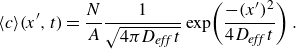 \begin{equation} \langle c\rangle (x^{\prime},t)=\frac{N}{A}\frac{1}{\sqrt{4\pi D_{\textit{eff}}\,t}}\exp\!\left(\frac{-(x^{\prime})^{2}}{4D_{\textit{eff}}\,t}\right) .\end{equation}
This solution can be interpreted as the Green’s function (also know as heat kernel) for (3.17) which, as we discuss in the next section, can be used to construct a wide variety of solutions for more complex initial conditions. Further, the first derivative of (3.23) with respect to axial dimension is
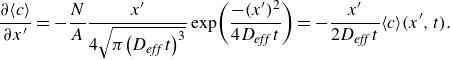 \begin{equation} \frac{\partial \!\left\langle c\right\rangle }{\partial x^{\prime}}=-\frac{N}{A}\frac{x^{\prime}}{4\sqrt{\pi \!\left(D_{\textit{eff}}\,t\right)^{3}}}\exp\!\left(\frac{-(x^{\prime})^{2}}{4D_{\textit{eff}}\,t}\right)=-\frac{x^{\prime}}{2D_{\textit{eff}}\,t}\!\left\langle c\right\rangle \! (x^{\prime},t) .\end{equation}
Equations (3.23) and (3.24) can be combined with (3.11) to obtain a solution of the full two-dimensional, unsteady solute concentration for a delta function initial condition as follows:
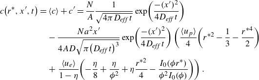 \begin{align} c\!\left(r^{*},x^{\prime},t\right)&=\left\langle c\right\rangle +c^{\prime}=\frac{N}{A}\frac{1}{\sqrt{4\pi D_{\textit{eff}}\,t}}\exp\!\left(\frac{-(x^{\prime})^{2}}{4D_{\textit{eff}}\,t}\right)\nonumber\\&\quad - \frac{Na^{2}x^{\prime}}{4AD\sqrt{\pi \!\left(D_{\textit{eff}}\,t\right)^{3}}}\exp\!\left(\frac{-(x^{\prime})^{2}}{4D_{\textit{eff}}\,t}\right)\left(\frac{ \langle u_{p}\rangle }{4}\!\left(r^{*2}-\frac{1}{3}-\frac{r^{*4}}{2}\right)\right.\nonumber\\&\quad +\left.\frac{\left\langle u_{e}\right\rangle }{1-\eta }\!\left(-\frac{\eta }{8}+\frac{\eta }{\phi ^{2}}+\eta \frac{r^{*2}}{4}-\frac{I_{0}\!\left(\phi r^{*}\right)}{\phi ^{2}I_{0}\!\left(\phi \right)}\right)\right). \end{align}
To our knowledge, (3.25) is the first reported expression which provides both the axial and radial distribution of solute for combined EOF and PDF.
3.1. Unsteady, two-dimensional solutions for arbitrary initial conditions
Given the linearity of (3.17), we leverage a Green’s function to present the concentration field as a function of arbitrary initial conditions. The Green’s function for this case is the solution of (3.17) for a delta function initial condition (Cole Reference Cole2011). From (3.23), the Green’s function is
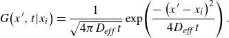 \begin{equation} G\!\left(x^{\prime},t|x_{i}\right)=\frac{1}{\sqrt{4\pi D_{\textit{eff}}\,t}}\exp\!\left(\frac{-\left(x^{\prime}-x_{i}\right)^{2}}{4D_{\textit{eff}}\,t}\right) .\end{equation}
Whence, combining with (3.11), we construct the solution to some arbitrary initial condition $\langle c\rangle (x^{\prime},0)$
as follows:
$\langle c\rangle (x^{\prime},0)$
as follows:
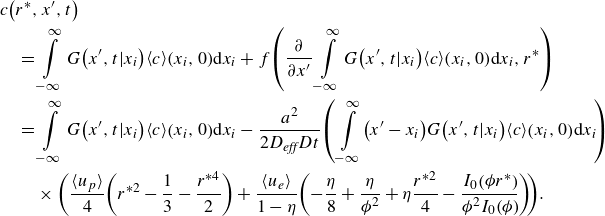 \begin{align} &c\!\left(r^{*},x^{\prime},t\right)\nonumber \\&\quad =\int\limits_{-\infty }^{\infty }G\!\left(x^{\prime},t|x_{i}\right)\!\left\langle c\right\rangle \!\left(x_{i},0\right)\!\mathrm{d}x_{i} +f\!\left(\frac{\partial }{\partial x^{\prime}}\int\limits_{-\infty }^{\infty }G\!\left(x^{\prime},t|x_{i}\right)\!\left\langle c\right\rangle \!\left(x_{i},0\right)\! \mathrm{d}x_{i},r^{*}\right)\nonumber\\&\quad = \int\limits_{-\infty }^{\infty }G\!\left(x^{\prime},t|x_{i}\right)\!\left\langle c\right\rangle \!\left(x_{i},0\right)\! \mathrm{d}x_{i} -\frac{a^{2}}{2D_{\textit{eff}}Dt}\!\left(\int\limits_{\,-\infty }^{\infty }\!\left(x^{\prime}-x_{i}\right)\!G\!\left(x^{\prime},t|x_{i}\right)\! \left\langle c\right\rangle \!\left(x_{i},0\right)\! \mathrm{d}x_{i}\!\right)\nonumber\\&\qquad \times \left(\frac{ \langle u_{p} \rangle }{4}\!\left(r^{*2}-\frac{1}{3}-\frac{r^{*4}}{2}\right)+\frac{\left\langle u_{e}\right\rangle }{1-\eta }\!\left(-\frac{\eta }{8}+\frac{\eta }{\phi ^{2}}+\eta \frac{r^{*2}}{4}-\frac{I_{0}\!\left(\phi r^{*}\right)\!}{\phi ^{2}I_{0}\!\left(\phi \right)\!}\right)\!\right)\!. \end{align}
3.2. Variance growth valid for any initial condition
We derive a general expression for the growth of the solute area-averaged variance valid for any initial condition. Let $v_{2}$
denote the axial variance of the solute about the axial mean defined such that
$v_{2}$
denote the axial variance of the solute about the axial mean defined such that
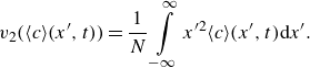 \begin{equation} v_{2}(\langle c \rangle \kern2pt \!(x',t)) = \frac{1}{N}\int\limits _{-\infty }^{\infty }x^{\prime2}\!\left\langle c\right\rangle \! (x^{\prime},t)\mathrm{d}x^{\prime} .\end{equation}
Equation (3.28) can be expressed in terms of $G(x^{\prime},t|x_{i})$
as follows:
$G(x^{\prime},t|x_{i})$
as follows:
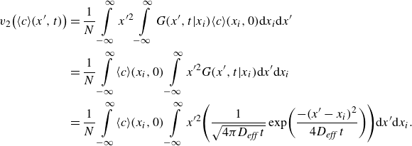 \begin{align} v_{2}\!\left(\left\langle c\right\rangle \!(x^{\prime},t)\right)&=\frac{1}{N}\int\limits_{-\infty }^{\infty }x^{\prime2}\int\limits_{-\infty }^{\infty }G (x^{\prime},t|x_{i})\!\left\langle c\right\rangle \!\left(x_{i},0\right)\!\mathrm{d}x_{i}\mathrm{d}x^{\prime}\nonumber\\&= \frac{1}{N}\int\limits_{-\infty }^{\infty }\!\left\langle c\right\rangle \!\left(x_{i},0\right)\int\limits_{-\infty }^{\infty }x^{\prime2}G (x^{\prime},t|x_{i}) \mathrm{d}x^{\prime}\mathrm{d}x_{i}\nonumber\\&= \frac{1}{N}\int\limits_{-\infty }^{\infty }\!\left\langle c\right\rangle \!\left(x_{i},0\right)\int\limits_{-\infty }^{\infty }x^{\prime2}\!\left(\frac{1}{\sqrt{4\pi D_{\textit{eff}}\,t}}\exp\!\left(\frac{-(x^{\prime}-x_{i})^{2}}{4D_{\textit{eff}}\,t}\right)\right)\!\mathrm{d}x^{\prime} \mathrm{d}x_{i}. \end{align}
We recognise the last interior integral as the second moment of a Gaussian with mean $x_{i}$
and variance
$x_{i}$
and variance $2D_{\textit{eff}}\,t$
. This implies
$2D_{\textit{eff}}\,t$
. This implies
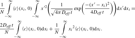 \begin{align} &\frac{1}{N}\int\limits_{-\infty }^{\infty }\!\left\langle c\right\rangle \!\left(x_{i},0\right)\int\limits_{-\infty }^{\infty }x^{\prime2}\!\left(\frac{1}{\sqrt{4\pi D_{\textit{eff}}\,t}}\exp\!\left(\frac{-(x^{\prime}-x_{i})^{2}}{4D_{\textit{eff}}\,t}\right)\right)\!\mathrm{d}x^{\prime}\mathrm{d}x_{i}=\nonumber\\ & \frac{2D_{\textit{eff}}\,t}{N}\int\limits_{-\infty }^{\infty }\!\left\langle c\right\rangle \!\left(x_{i},0\right)\!\mathrm{d}x_{i}+\frac{1}{N}\int\limits_{-\infty }^{\infty }{x_{i}}^{2}\!\left\langle c\right\rangle \!\left(x_{i},0\right)\!\mathrm{d}x_{i}. \end{align}
Therefore, variance grows as
 \begin{equation} v_{2}(\left\langle c\right\rangle \! (x^{\prime},t))=2D_{\textit{eff}}\,t+v_{2}(\langle c\rangle \kern2pt \!(x^{\prime},0)) .\end{equation}
That is, the solute variance for all time is simply the sum of its initial value and $2D_{\textit{eff}}\,t$
.
$2D_{\textit{eff}}\,t$
.
3.3. Minimisation of variance for transporting solute over arbitrary axial distances
We here derive analytical expressions and present methods to minimise the axial variance of solute as it is transported over an arbitrary, non-zero axial distance. As such, we do not consider the case of $\langle u\rangle =0$
(e.g. wherein EOF and PDF are perfectly opposed), ensuring the parameter
$\langle u\rangle =0$
(e.g. wherein EOF and PDF are perfectly opposed), ensuring the parameter $\beta =\langle u_{p}\rangle /\langle u\rangle$
remains finite.
$\beta =\langle u_{p}\rangle /\langle u\rangle$
remains finite.
First, we consider the relatively rare case where the practitioner can vary the relative EDL thickness ( $\phi$
) as is possible in some nanochannel systems. To minimise variance growth, the EDL should be made as relatively thin as possible (
$\phi$
) as is possible in some nanochannel systems. To minimise variance growth, the EDL should be made as relatively thin as possible ( $\phi \rightarrow \infty$
) as this minimises dispersion.
$\phi \rightarrow \infty$
) as this minimises dispersion.
The fraction of bulk velocity associated with pressure required to minimise the growth of the solute variance, $\beta _{o}$
, as a function of the tube radius scaled by Debye length,
$\beta _{o}$
, as a function of the tube radius scaled by Debye length, $\phi$
. The inset shows the variance-minimising normalised flow profiles,
$\phi$
. The inset shows the variance-minimising normalised flow profiles, $\hat{u}_{o}(r^{*})$
, for select values of
$\hat{u}_{o}(r^{*})$
, for select values of $\phi$
of 1, 5, 10, 25 and 50. Opposing EOF with PDF can be used to suppress dispersion.
$\phi$
of 1, 5, 10, 25 and 50. Opposing EOF with PDF can be used to suppress dispersion.
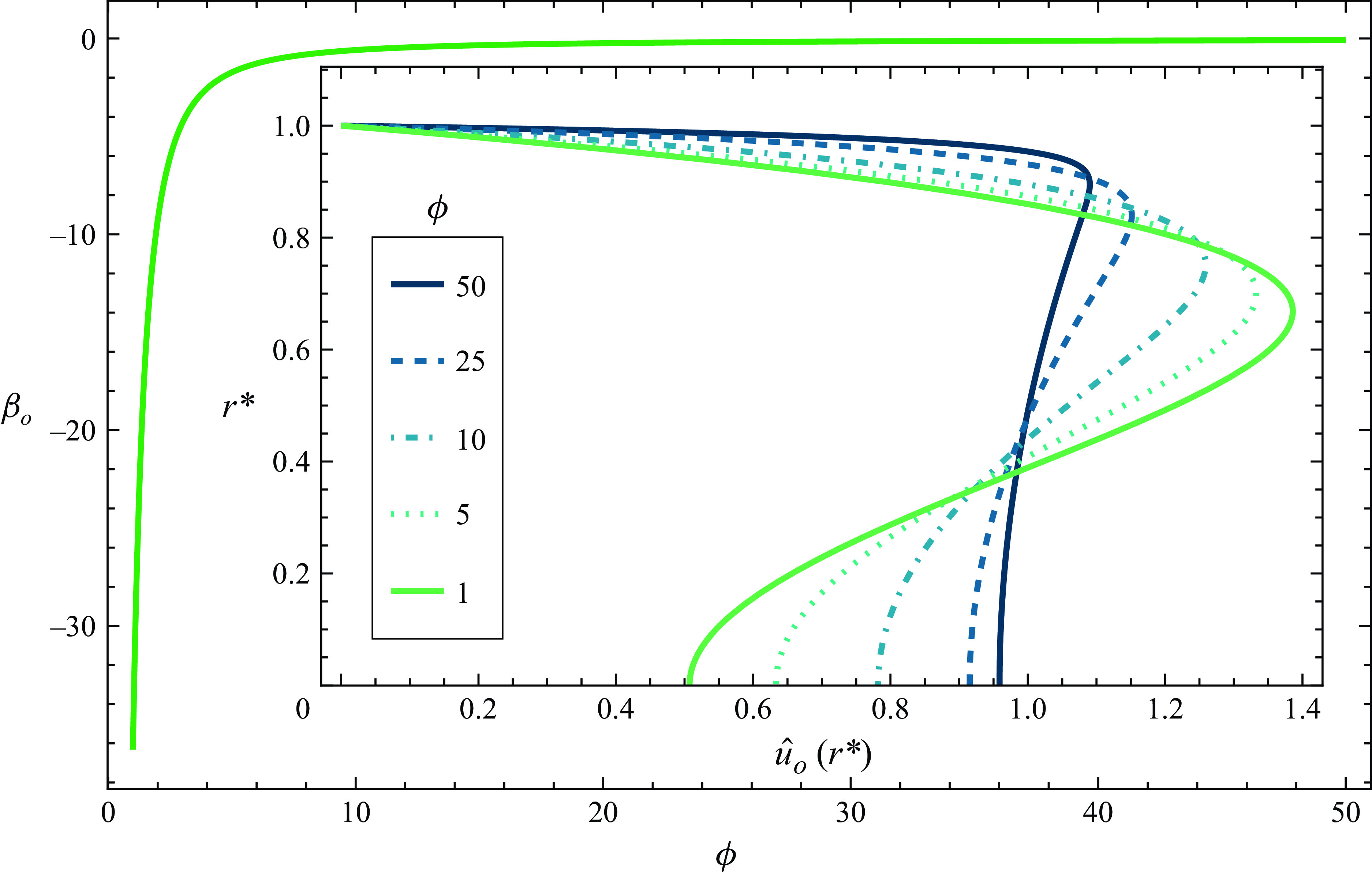
Next, we consider a more practical situation. Assume the channel geometry and Debye length of a system are fixed. This fixes the relative EDL thickness $\phi$
. To minimise variance, (3.20) shows that we should consider both
$\phi$
. To minimise variance, (3.20) shows that we should consider both $\beta$
and
$\beta$
and $\textit{Pe}$
. From (3.31), we see that minimisation of variance in terms of the parameter
$\textit{Pe}$
. From (3.31), we see that minimisation of variance in terms of the parameter $\beta$
implies a minimisation of
$\beta$
implies a minimisation of $D_{\textit{eff}}$
. We proceed by taking the partial derivative of (3.20) with respect to
$D_{\textit{eff}}$
. We proceed by taking the partial derivative of (3.20) with respect to $\beta$
and setting the resulting expression equal to zero. The variance-minimising value of
$\beta$
and setting the resulting expression equal to zero. The variance-minimising value of $\beta$
, denoted here as
$\beta$
, denoted here as $\beta _{o}$
, is then
$\beta _{o}$
, is then
 \begin{equation} \beta _{o}=\frac{\gamma _{pe}-2\gamma _{e}}{2\left(\gamma _{pe}-\gamma _{e}-\gamma _{p}\right)} .\end{equation}
Interestingly, and somewhat counterintuitively, we find that $\beta _{o}$
is determined completely by
$\beta _{o}$
is determined completely by $\phi$
and is independent of
$\phi$
and is independent of $P\hspace{0pt}e$
. For any one value
$P\hspace{0pt}e$
. For any one value $\phi$
, there is a unique combination of EOF and PDF which minimises variance and is applicable to all bulk velocities, tube radii and solute diffusivities (which determine
$\phi$
, there is a unique combination of EOF and PDF which minimises variance and is applicable to all bulk velocities, tube radii and solute diffusivities (which determine $P\hspace{0pt}e$
). We shall see that this optimum velocity profile shape is achieved by opposing EOF with progressively stronger PDF as the EDL becomes thicker (we will discuss this further when presenting figure 9). Datta & Kotamarthi (Reference Datta and Kotamarthi1990) also identified this optimum
$P\hspace{0pt}e$
). We shall see that this optimum velocity profile shape is achieved by opposing EOF with progressively stronger PDF as the EDL becomes thicker (we will discuss this further when presenting figure 9). Datta & Kotamarthi (Reference Datta and Kotamarthi1990) also identified this optimum $\beta _{o}$
(see equation (50) of Datta & Kotamarthi Reference Datta and Kotamarthi1990). However, we note that Datta & Kotamarthi focused their presentation on the minimisation of the theoretical plate height. Theoretical plate heights are traditional figures of merit for species separation systems, including electrophoresis and chromatography, which aim to capture the number of peaks detectable using a certain column (i.e. channel) length (see Huang Reference Huang2021). We here will instead focus on the more fundamental problem of minimising
$\beta _{o}$
(see equation (50) of Datta & Kotamarthi Reference Datta and Kotamarthi1990). However, we note that Datta & Kotamarthi focused their presentation on the minimisation of the theoretical plate height. Theoretical plate heights are traditional figures of merit for species separation systems, including electrophoresis and chromatography, which aim to capture the number of peaks detectable using a certain column (i.e. channel) length (see Huang Reference Huang2021). We here will instead focus on the more fundamental problem of minimising $D_{\textit{eff}}$
and axial variance. Lastly, we henceforth denote the flow profile based on a value of
$D_{\textit{eff}}$
and axial variance. Lastly, we henceforth denote the flow profile based on a value of $\beta =\beta _{o}$
as
$\beta =\beta _{o}$
as $u_{o}(r^{*})$
(and define
$u_{o}(r^{*})$
(and define $\hat{u}_{o}(r^{*})=u_{o}(r^{*})/\langle u\rangle$
).
$\hat{u}_{o}(r^{*})=u_{o}(r^{*})/\langle u\rangle$
).
Next, we explore the effects of flow Péclet number on the minimum dispersion conditions. From (3.31), assuming some negligible initial width of the solute (compared with its final value), the final variance of the solute cloud reduces simply to $2D_{\textit{eff}}\,t$
. First, we non-dimensionalise the solute variance as
$2D_{\textit{eff}}\,t$
. First, we non-dimensionalise the solute variance as $2D_{\textit{eff}}^{*}\tau =2D_{\textit{eff}}\,t/a^{2}$
, where
$2D_{\textit{eff}}^{*}\tau =2D_{\textit{eff}}\,t/a^{2}$
, where $\tau =tD/a^{2}$
is the dimensionless time. We wish to minimise
$\tau =tD/a^{2}$
is the dimensionless time. We wish to minimise $2D_{\textit{eff}}^{*}\tau$
for some finite distance travelled
$2D_{\textit{eff}}^{*}\tau$
for some finite distance travelled $L$
or, in dimensionless form,
$L$
or, in dimensionless form, $L^{*}=L/a$
. To proceed, we first multiply (3.20) by the dimensionless time
$L^{*}=L/a$
. To proceed, we first multiply (3.20) by the dimensionless time $\tau =L^{*}/\textit{Pe}$
 \begin{equation} \frac{L^{*}}{\textit{Pe}}D_{\textit{eff}}^{*}=\frac{L^{*}}{\textit{Pe}}+L^{*}P\hspace{0pt}e\left(\beta ^{2}\gamma _{p}+\beta \left(1-\beta \right)\gamma _{pe}+\left(1-\beta \right)^{2}\gamma _{e}\right) .\end{equation}
We differentiate the right-hand side of (3.33) with respect to $P\hspace{0pt}e$
and set this equal to zero
$P\hspace{0pt}e$
and set this equal to zero
 \begin{equation} -\frac{L^{*}}{\textit{Pe}^{2}}+L^{*}\!\left(\beta ^{2}\gamma _{p}+\beta \left(1-\beta \right)\gamma _{pe}+\left(1-\beta \right)^{2}\gamma _{e}\right)=0 .\end{equation}
Recall we here assume $\textit{Pe}\neq 0$
. Multiplying (3.34) by
$\textit{Pe}\neq 0$
. Multiplying (3.34) by $P\hspace{0pt}e^{2}$
, the roots of the resulting equation can be expressed as
$P\hspace{0pt}e^{2}$
, the roots of the resulting equation can be expressed as
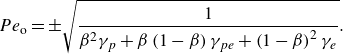 \begin{equation} P\hspace{0pt}e_{\mathrm{o}}=\pm \sqrt{\frac{1}{\beta ^{2}\gamma _{p}+\beta \left(1-\beta \right)\gamma _{pe}+\left(1-\beta \right)^{2}\gamma _{e}}} .\end{equation}
This compact expression yields the Péclet number that minimises the rate of growth of the variance per unit of axial distance travelled. Since we assumed a negligible initial width of the solute, the resulting variance-minimising $\textit{Pe}$
is independent of
$\textit{Pe}$
is independent of $L^{*}$
. Note the
$L^{*}$
. Note the $\pm$
simply reflects the symmetry of the system for bulk velocities in the ‘positive’ or ‘negative’ direction and can therefore be discarded. Equation (3.35) then provides the optimum Péclet number to minimise variance for transporting solute for any values of the parameters
$\pm$
simply reflects the symmetry of the system for bulk velocities in the ‘positive’ or ‘negative’ direction and can therefore be discarded. Equation (3.35) then provides the optimum Péclet number to minimise variance for transporting solute for any values of the parameters $\beta$
and
$\beta$
and $\phi$
. If one considers variations of
$\phi$
. If one considers variations of $\beta$
(i.e. adjustments of the relative strength of EOF and PDF), then the substitution of (3.32) into (3.35) conveniently reduces
$\beta$
(i.e. adjustments of the relative strength of EOF and PDF), then the substitution of (3.32) into (3.35) conveniently reduces $P\hspace{0pt}e_{\mathrm{o}}$
to a function of only the fixed parameter
$P\hspace{0pt}e_{\mathrm{o}}$
to a function of only the fixed parameter $\phi$
. If instead
$\phi$
. If instead $\beta$
is taken to be fixed, then (3.35) provides
$\beta$
is taken to be fixed, then (3.35) provides $P\hspace{0pt}e_{\mathrm{o}}$
as a function of both
$P\hspace{0pt}e_{\mathrm{o}}$
as a function of both $\phi$
and the value of
$\phi$
and the value of $\beta$
. In either case, the relations
$\beta$
. In either case, the relations $\beta \textit{Pe}=\textit{Pe}_{p}$
and
$\beta \textit{Pe}=\textit{Pe}_{p}$
and $(1-\beta )\textit{Pe}=\textit{Pe}_{e}$
can be used to find the variance-minimising PDF and EOF components once
$(1-\beta )\textit{Pe}=\textit{Pe}_{e}$
can be used to find the variance-minimising PDF and EOF components once $P\hspace{0pt}e_{\mathrm{o}}$
is known.
$P\hspace{0pt}e_{\mathrm{o}}$
is known.
We note that (3.35) may be interpreted as the variance-minimising ratio of advective to diffusive flux for transporting solute. In regimes where advection only slightly increases dispersion (e.g. dominant EOF with a thin EDL), the dispersion is dominated by molecular diffusion. In such regimes, the time to transport solute should then be minimised by increasing the EOF velocity and $\textit{Pe}$
. Hence,
$\textit{Pe}$
. Hence, $P\hspace{0pt}e_{\mathrm{o}}$
will be large for such velocity fields. We shall show (in the discussion of figure 10) that, for finite
$P\hspace{0pt}e_{\mathrm{o}}$
will be large for such velocity fields. We shall show (in the discussion of figure 10) that, for finite $\phi, P\hspace{0pt}e_{\mathrm{o}}$
achieves a maximum (with respect to
$\phi, P\hspace{0pt}e_{\mathrm{o}}$
achieves a maximum (with respect to $\beta$
) at the variance-minimising combination of EOF and PDF,
$\beta$
) at the variance-minimising combination of EOF and PDF, $\beta _{o}$
. To demonstrate this, we differentiate (3.35) with respect to
$\beta _{o}$
. To demonstrate this, we differentiate (3.35) with respect to $\beta$
and set the resulting quantity equal to zero
$\beta$
and set the resulting quantity equal to zero
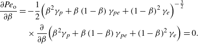 \begin{align} \frac{\partial \textit{Pe}_{\mathrm{o}}}{\partial \beta }&=-\frac{1}{2}\!\left(\beta ^{2}\gamma _{p}+\beta \left(1-\beta \right)\gamma _{pe}+\left(1-\beta \right)^{2}\gamma _{e}\right)^{-\frac{3}{2}}\nonumber\\&\quad\times\frac{\partial }{\partial \beta }\!\left(\beta ^{2}\gamma _{p}+\beta \left(1-\beta \right)\gamma _{pe}+\left(1-\beta \right)^{2}\gamma _{e}\right)=0 .\end{align}
Surface plots for analytical solutions of the quasi-steady state, variance-minimising Péclet number, $\textit{Pe}_{o}$
. In
$\textit{Pe}_{o}$
. In $(a)$
, a surface of
$(a)$
, a surface of $\textit{Pe}_{o}$
is plotted as a function of the fraction of bulk velocity caused by pressure,
$\textit{Pe}_{o}$
is plotted as a function of the fraction of bulk velocity caused by pressure, $\beta$
, and the tube radius scaled by Debye length,
$\beta$
, and the tube radius scaled by Debye length, $\phi$
. For constant values of
$\phi$
. For constant values of $\phi, \textit{Pe}_{o}$
exhibits a maximum at the aforementioned variance-minimising fraction of bulk velocity caused by pressure,
$\phi, \textit{Pe}_{o}$
exhibits a maximum at the aforementioned variance-minimising fraction of bulk velocity caused by pressure, $\beta _{o}$
. In
$\beta _{o}$
. In $(b)$
, a surface of
$(b)$
, a surface of $2D_{\textit{eff}}^{*}\tau$
is plotted for solute travelling an example dimensionless axial distance of
$2D_{\textit{eff}}^{*}\tau$
is plotted for solute travelling an example dimensionless axial distance of $L^{*}=\tau \textit{Pe}=50$
as a function of
$L^{*}=\tau \textit{Pe}=50$
as a function of $\beta$
and
$\beta$
and $P\hspace{0pt}e$
. Here, the white circle indicates the minimum of
$P\hspace{0pt}e$
. Here, the white circle indicates the minimum of $2D_{\textit{eff}}^{*}\tau$
as determined analytically by (3.32) and (3.35). Figure 10(b) was produced with an example relative EDL thickness of
$2D_{\textit{eff}}^{*}\tau$
as determined analytically by (3.32) and (3.35). Figure 10(b) was produced with an example relative EDL thickness of $\phi =50$
.
$\phi =50$
.
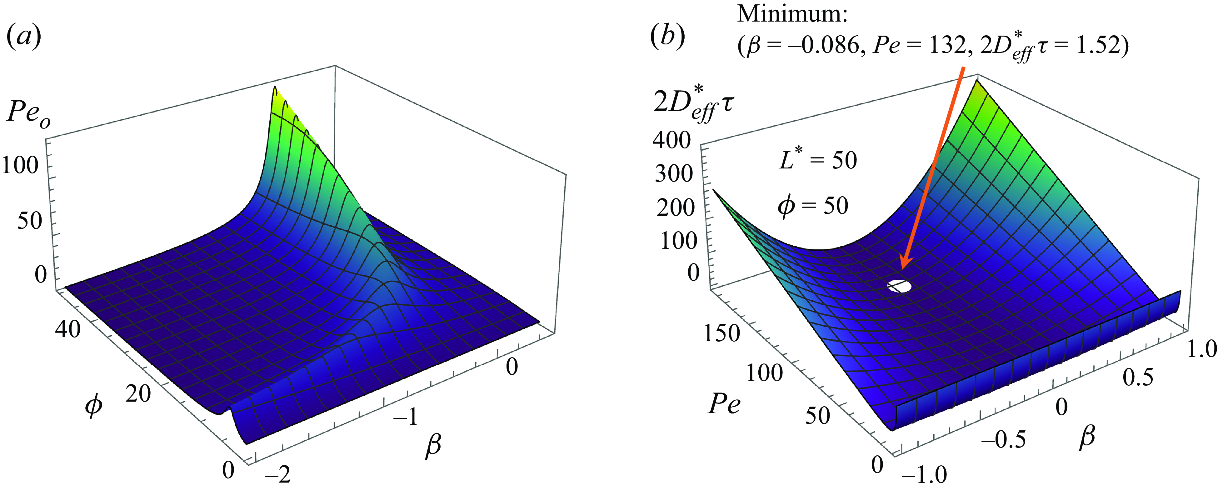
The prefactor parenthetic term on the right-hand side (raised to $-3/2$
) is always non-zero. Therefore, the right-hand side of (3.36) vanishes only when
$-3/2$
) is always non-zero. Therefore, the right-hand side of (3.36) vanishes only when $\beta =\beta _{o}$
. Hence, we conclude that (at a fixed value of
$\beta =\beta _{o}$
. Hence, we conclude that (at a fixed value of $\phi$
) the
$\phi$
) the $P\hspace{0pt}e_{\mathrm{o}}$
function achieves a maximum at
$P\hspace{0pt}e_{\mathrm{o}}$
function achieves a maximum at $\beta _{o}$
.
$\beta _{o}$
.
Lastly, we note that our (3.35) is mathematically equivalent to Datta & Kotamarthi’s (Reference Datta and Kotamarthi1990) equation (51). However, we again point out that Datta & Kotamarthi derived their optimal $\textit{Pe}$
by minimising the theoretical plate height (and we here do not need to invoke such figures of merit).
$\textit{Pe}$
by minimising the theoretical plate height (and we here do not need to invoke such figures of merit).
3.4. Example solution for a ‘top hat’ initial condition
In the case of an initial ‘top hat’ of solute, centred at $x^{\prime}=0$
, the initial conditions are
$x^{\prime}=0$
, the initial conditions are
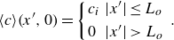 \begin{equation} \langle c\rangle (x^{\prime},0)=\left\{\begin{array}{ll} c_{i} & | x^{\prime}| \leq L_{o}\\[4pt] 0 & | x^{\prime}| \gt L_{o} \end{array}\right. .\end{equation}
Here, $c_{i}$
denotes the initial concentration of solute (with units of moles per litre) and
$c_{i}$
denotes the initial concentration of solute (with units of moles per litre) and $L_{o}$
denotes half of the initial width of the ‘top hat’. First, we compute the convolution of this initial condition with Green’s function as
$L_{o}$
denotes half of the initial width of the ‘top hat’. First, we compute the convolution of this initial condition with Green’s function as
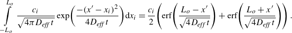 \begin{equation} \int\limits_{-L_{o}}^{L_{o}}\frac{c_{i}}{\sqrt{4\pi D_{\textit{eff}}\,t}}\exp\!\left(\frac{-(x^{\prime}-x_{i})^{2}}{4D_{\textit{eff}}\,t}\right)\!\mathrm{d}x_{i}=\frac{c_{i}}{2}\!\left(\mathrm{erf}\!\left(\frac{L_{o}-x^{\prime}}{\sqrt{4D_{\textit{eff}}\,t}}\right)+\mathrm{erf}\!\left(\frac{L_{o}+x^{\prime}}{\sqrt{4D_{\textit{eff}}\,t}}\right)\right) .\end{equation}
For the radial distribution of solute, we calculate
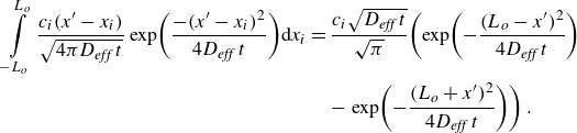 \begin{align} \int\limits_{-L_{o}}^{L_{o}}\frac{c_{i} (x^{\prime}-x_{i})}{\sqrt{4\pi D_{\textit{eff}}\,t}}\exp\!\left(\frac{-(x^{\prime}-x_{i})^{2}}{4D_{\textit{eff}}\,t}\right)\!\mathrm{d}x_{i}&=\frac{c_{i}\sqrt{D_{\textit{eff}}\,t}}{\sqrt{\pi }}\!\left(\exp\!\left(-\frac{(L_{o}-x^{\prime})^{2}}{4D_{\textit{eff}}\,t}\right)\right.\nonumber\\&\quad-\left.\exp\!\left(-\frac{(L_{o}+x^{\prime})^{2}}{4D_{\textit{eff}}\,t}\right)\right) .\end{align}
Substituting (3.38) and (3.39) into (3.27), we see that, in the ‘top hat’ case, the overall concentration field can be expressed as
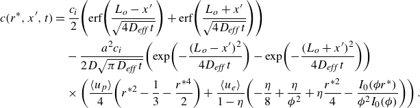 \begin{align} c(r^{*},x^{\prime},t)&= \frac{c_{i}}{2}\!\left(\mathrm{erf}\!\left(\frac{L_{o}-x^{\prime}}{\sqrt{4D_{\textit{eff}}\,t}}\right)+\mathrm{erf}\!\left(\frac{L_{o}+x^{\prime}}{\sqrt{4D_{\textit{eff}}\,t}}\right)\right)\nonumber\\ &\quad-\frac{a^{2}c_{i}}{2D\sqrt{\pi D_{\textit{eff}}\,t}}\!\left(\exp\!\left(-\frac{(L_{o}-x^{\prime})^{2}}{4D_{\textit{eff}}\,t}\right)-\exp\!\left(-\frac{(L_{o}+x^{\prime})^{2}}{4D_{\textit{eff}}\,t}\right)\right)\nonumber\\ &\quad\times \left(\frac{\langle u_{p}\rangle }{4}\!\left(r^{*2}-\frac{1}{3}-\frac{r^{*4}}{2}\right)+\frac{\left\langle u_{e}\right\rangle }{1-\eta }\!\left(-\frac{\eta }{8}+\frac{\eta }{\phi ^{2}}+\eta \frac{r^{*2}}{4}-\frac{I_{0}\!\left(\phi r^{*}\right)}{\phi ^{2}I_{0}\!\left(\phi \right)}\right)\right). \end{align}
Again, (3.40) is valid for the Taylor-type limit of the problem (cf. (3.4) and (3.5)).
4. Method of moments solution for transient dispersive behaviour
We present a solution for the integral moments of the solute zone which is valid for all times. Our solution will also be valid for solute zones with arbitrary axial widths. We follow the MoM solution method originated by Aris (Reference Aris1956), as significantly expanded and developed by Barton (Reference Barton1983). Barton advanced the MoM by employing eigenfunction expansions from Sturm–Liouville theory to derive general expressions for the integral moments of the concentration field. Barton’s analysis applies to arbitrary flow profiles and arbitrary channel cross-sections. We will here use Barton’s general framework to analyse the behaviour of solute subject to coupled EOF and PDF in a cylindrical tube. We note there are several key differences between our MoM formulation and our quasi-steady, Taylor-type analysis from § 3. First, the conditions $\textit{Pe}\lt \lt \sigma _{x}/a$
and
$\textit{Pe}\lt \lt \sigma _{x}/a$
and $a/\sigma _{x}\lt \lt 1$
are not required for our MoM formulation. Second, consistent with the MoM, we non-dimensionalise axial position with the inner radius of the tube and not the characteristic width of the solute cloud (
$a/\sigma _{x}\lt \lt 1$
are not required for our MoM formulation. Second, consistent with the MoM, we non-dimensionalise axial position with the inner radius of the tube and not the characteristic width of the solute cloud ( $x^{*}=x/a$
). Third, we non-dimensionalise the concentration field with the total moles of solute in the tube and the characteristic volume of the tube (
$x^{*}=x/a$
). Third, we non-dimensionalise the concentration field with the total moles of solute in the tube and the characteristic volume of the tube ( $c^{*}(r^{*},x^{*},\tau )=\pi a^{3}c(r^{*},x^{*},\tau )/N$
). Lastly, we non-dimensionalise our velocity profile as follows:
$c^{*}(r^{*},x^{*},\tau )=\pi a^{3}c(r^{*},x^{*},\tau )/N$
). Lastly, we non-dimensionalise our velocity profile as follows:
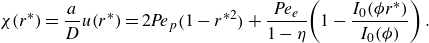 \begin{equation} \chi (r^{*})=\frac{a}{D}u (r^{*})=2\textit{Pe}_{p}\big(1-r^{*2}\big)+\frac{\textit{Pe}_{e}}{1-\eta }\!\left(1-\frac{I_{0}\!\left(\phi r^{*}\right)}{I_{0}\!\left(\phi \right)}\right) .\end{equation}
The latter can be interpreted as a Péclet number in terms of the (radially varying) velocity profile. In terms of these newly defined variables, the dimensionless convection–diffusion equation and boundary conditions are
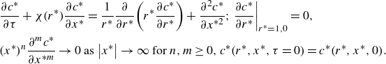 \begin{align} &\frac{\partial c^{*}}{\partial \tau }+\chi (r^{*})\frac{\partial c^{*}}{\partial x^{*}}=\frac{1}{r^{*}}\frac{\partial }{\partial r^{*}}\!\left(r^{*}\frac{\partial c^{*}}{\partial r^{*}}\right)+\frac{\partial ^{2}c^{*}}{\partial x^{*2}}; \left.\frac{\partial c^{*}}{\partial r^{*}}\right| _{r^{*}=1,0}=0,\nonumber\\ & (x^{*})^{n}\frac{\partial ^{m}c^{*}}{\partial x^{*m}}\rightarrow 0\text{ as }\!\left| x^{*}\right| \rightarrow \infty \text{ for }n, m\geq 0,c^{*}(r^{*},x^{*},\tau =0)=c^{*}(r^{*},x^{*},0). \end{align}
Defining $c _{n}^{*}(r^{*},\tau )=\int _{-\infty }^{\infty }(x^{*})^{n}c^{*}(r^{*},x^{*},\tau )\mathrm{d}x^{*}$
as the nth moment of solute along the axial direction, we can multiply (4.2) by
$c _{n}^{*}(r^{*},\tau )=\int _{-\infty }^{\infty }(x^{*})^{n}c^{*}(r^{*},x^{*},\tau )\mathrm{d}x^{*}$
as the nth moment of solute along the axial direction, we can multiply (4.2) by $(x^*)^{n}$
and integrate with respect to
$(x^*)^{n}$
and integrate with respect to $x^{*}$
, yielding
$x^{*}$
, yielding
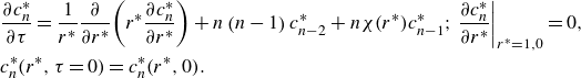 \begin{align} &\frac{\partial c _{n}^{*}}{\partial \tau }=\frac{1}{r^{*}}\frac{\partial }{\partial r^{*}}\!\left(r^{*}\frac{\partial c _{n}^{*}}{\partial r^{*}}\right)+n\left(n-1\right)c _{n-2}^{*}+n \chi (r^{*})c _{n-1}^{*};\left.\frac{\partial c _{n}^{*}}{\partial r^{*}}\right| _{r^{*}=1,0}=0,\nonumber\\ & c _{n}^{*}(r^{*},\tau =0)=c _{n}^{*}(r^{*},0). \end{align}
Taking an area average of (4.3)
 \begin{equation} \frac{dM_{n}}{d\tau }=n\left(n-1\right)\langle c _{n-2}^{*} \rangle +n \langle \chi (r^{*})c _{n-1}^{*} \rangle ;\, M_{n}\!\left(\tau =0\right)=M_{n}\!\left(0\right) .\end{equation}
Here, $M_{n}(\tau )=\int _{0}^{1}2r^{*}c _{n}^{*}(r^{*},\tau )\mathrm{d}r^{*}$
and
$M_{n}(\tau )=\int _{0}^{1}2r^{*}c _{n}^{*}(r^{*},\tau )\mathrm{d}r^{*}$
and $M_{n}(0)$
are respectively the nth moment of the solute zone and the initial value of the nth moment of solute. Equation (4.4) is then the governing initial value problem for the nth moment of the concentration field. We note that solutions from (4.4) for the nth moment of solute depend upon the solutions of
$M_{n}(0)$
are respectively the nth moment of the solute zone and the initial value of the nth moment of solute. Equation (4.4) is then the governing initial value problem for the nth moment of the concentration field. We note that solutions from (4.4) for the nth moment of solute depend upon the solutions of $c _{n-1}^{*}(r^{*},\tau )$
and
$c _{n-1}^{*}(r^{*},\tau )$
and $c _{n-2}^{*}(r^{*},\tau )$
from (4.3). In this way, solutions for the higher-order moments of solute must be ‘built up’ from solutions of lower-order moments of solute along the axial direction. To this end, we will solve (4.3) with the method of separation of variables. Given the cylindrical geometry of our formulation, the Sturm–Liouville eigenvalue problem (Amrein, Hinz & Pearson Reference Amrein, Hinz and Pearson2005) associated with our solution method is
$c _{n-2}^{*}(r^{*},\tau )$
from (4.3). In this way, solutions for the higher-order moments of solute must be ‘built up’ from solutions of lower-order moments of solute along the axial direction. To this end, we will solve (4.3) with the method of separation of variables. Given the cylindrical geometry of our formulation, the Sturm–Liouville eigenvalue problem (Amrein, Hinz & Pearson Reference Amrein, Hinz and Pearson2005) associated with our solution method is
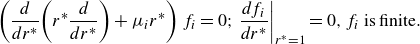 \begin{align} \left(\frac{d}{dr^{*}}\!\left(r^{*}\frac{d}{dr^{*}}\right)+\mu _{i}r^{*}\right)f_{i}=0;\left.\frac{df_{i}}{dr^{*}}\right| _{r^{*}=1}=0,f_{i}\,{\mathrm {is\,finite}}. \end{align}
The orthonormal eigenfunctions and discrete eigenvalues of (4.5) are
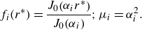 \begin{equation} f_{i} (r^{*})=\frac{J_{0}\!\left(\alpha _{i}r^{*}\right)}{J_{0}\!\left(\alpha _{i}\right)};\mu _{i}=\alpha _{i}^{2} .\end{equation}
Here, $J_{v}(z)$
denotes a Bessel function of the first kind of order
$J_{v}(z)$
denotes a Bessel function of the first kind of order $v$
, and
$v$
, and $\alpha _{i}$
is the ith root of
$\alpha _{i}$
is the ith root of $J_{1}(z)$
. As previously mentioned, Barton (Reference Barton1983) provided a general formulation of the first moment of the concentration field in terms of the eigenfunctions associated with arbitrary tube geometries and arbitrary velocity profiles. Importantly, Barton showed that the first moment of the concentration field satisfies the equation
$J_{1}(z)$
. As previously mentioned, Barton (Reference Barton1983) provided a general formulation of the first moment of the concentration field in terms of the eigenfunctions associated with arbitrary tube geometries and arbitrary velocity profiles. Importantly, Barton showed that the first moment of the concentration field satisfies the equation
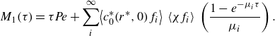 \begin{equation} M_{1}(\tau )=\tau \textit{Pe}+\sum _{i}^{\infty }\!\left\langle c _{0}^{*}(r^{*},0)f_{i}\right\rangle \,\left\langle \chi f_{i}\right\rangle \,\left(\frac{1-e^{-{\mu _{i}}\tau }}{\mu _{i}}\right) .\end{equation}
Without loss of generality, we have assumed that $M_{1}(0)=0$
. To apply Barton’s approach to the current geometry and velocity fields, we must evaluate the following eigenfunction-weighted area average of the velocity profile in (4.1)
$M_{1}(0)=0$
. To apply Barton’s approach to the current geometry and velocity fields, we must evaluate the following eigenfunction-weighted area average of the velocity profile in (4.1)
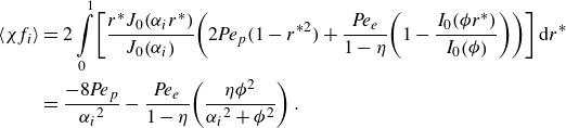 \begin{align} \left\langle \chi f_{i}\right\rangle &=2\int\limits_{0}^{1} \!\left[\frac{r^{*}J_{0} \big(\alpha _{i}r^{*}\big)}{J_{0}\!\left(\alpha _{i}\right)}\!\left(2\textit{Pe}_{p} \big(1-r^{*2}\big)+\frac{\textit{Pe}_{e}}{1-\eta }\!\left(1-\frac{I_{0}\!\left(\phi r^{*}\right)}{I_{0}\!\left(\phi \right)}\right)\right)\right]\mathrm{d}r^{*}\nonumber\\&=\frac{-8\textit{Pe}_{p}}{{\alpha _{i}}^{2}}-\frac{\textit{Pe}_{e}}{1-\eta }\!\left(\frac{\eta \phi ^{2}}{{\alpha _{i}}^{2}+\phi ^{2}}\right) .\end{align}
The substitution of (4.8) into (4.7) then provides the axial mean of the solute zone as a function of the eigenfunction-weighted area average of arbitrary initial conditions, $\langle c _{0}^{*}(r^{*},0)f_{i}\rangle$
.
$\langle c _{0}^{*}(r^{*},0)f_{i}\rangle$
.
In this work, we discuss the term $\langle c_{0}^{*}(r^{*},0)f_{i}\rangle$
for two interesting initial conditions. The first initial condition we will consider is the case of solute that is distributed uniformly across the cross-section of the tube. For such initial conditions
$\langle c_{0}^{*}(r^{*},0)f_{i}\rangle$
for two interesting initial conditions. The first initial condition we will consider is the case of solute that is distributed uniformly across the cross-section of the tube. For such initial conditions
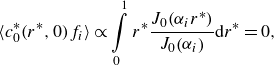 \begin{equation} \langle c _{0}^{*}(r^{*},0)f_{i}\rangle \propto \int\limits_{0}^{1}r^{*}\frac{J_{0}\!\left(\alpha _{i}r^{*}\right)}{J_{0}\!\left(\alpha _{i}\right)}\mathrm{d} r^{*}=0, \end{equation}
so (4.7) reduces to simply $M_{1}(\tau )=\tau \textit{Pe}$
(where
$M_{1}(\tau )=\tau \textit{Pe}$
(where $P\hspace{0pt}e$
is a signed quantity or zero). The latter reflects the fact that the solute zone (eventually) moves at the net bulk velocity of the flow. The second initial condition we will consider is an initial delta distribution of solute at
$P\hspace{0pt}e$
is a signed quantity or zero). The latter reflects the fact that the solute zone (eventually) moves at the net bulk velocity of the flow. The second initial condition we will consider is an initial delta distribution of solute at $r^{*}=0$
. From the definition of the delta distribution,
$r^{*}=0$
. From the definition of the delta distribution, $\langle c _{0}^{*}(r^{*},0)f_{i}\rangle =2J_{0}(0)/J_{0}(\alpha _{i})$
, whence
$\langle c _{0}^{*}(r^{*},0)f_{i}\rangle =2J_{0}(0)/J_{0}(\alpha _{i})$
, whence
 \begin{equation} M_{1}(\tau )=\tau \textit{Pe}+\sum _{i}^{\infty }\frac{2}{J_{0}\!\left(\alpha _{i}\right)}\!\left(\frac{-8\textit{Pe}_{p}}{{\alpha _{i}}^{2}}-\frac{\textit{Pe}_{e}}{1-\eta }\!\left(\frac{\eta \phi ^{2}}{{\alpha _{i}}^{2}+\phi ^{2}}\right)\right)\left(\frac{1-e^{-{{\alpha _{i}}^{2}}\tau }}{{\alpha _{i}}^{2}}\right) .\end{equation}
In the limit as $\tau \rightarrow \infty$
, (4.10) again reflects the fact that the solute zone ultimately moves at bulk velocity. Also, (4.10) shows that the mean of the solute cloud will in general deviate from that predicted by our quasi-steady solution. In most practical applications, this deviation is small and negligible. Further, in contrast to our quasi-steady solution, the mean axial location of the solute as predicted by this MoM formulation depends explicitly on the initial condition of solute. As per (4.9), this dependence vanishes for initial distributions of solute which are uniform across the cross-section of the tube, simplifying the problem of solving for higher-order moments of the solute zone. Given this, we shall only consider such initial conditions in our solution of the variance of the solute zone.
$\tau \rightarrow \infty$
, (4.10) again reflects the fact that the solute zone ultimately moves at bulk velocity. Also, (4.10) shows that the mean of the solute cloud will in general deviate from that predicted by our quasi-steady solution. In most practical applications, this deviation is small and negligible. Further, in contrast to our quasi-steady solution, the mean axial location of the solute as predicted by this MoM formulation depends explicitly on the initial condition of solute. As per (4.9), this dependence vanishes for initial distributions of solute which are uniform across the cross-section of the tube, simplifying the problem of solving for higher-order moments of the solute zone. Given this, we shall only consider such initial conditions in our solution of the variance of the solute zone.
Before continuing we explicitly write here the quasi-steady limits of (4.7) and (4.10) for the case of pure PDF. Substituting $\textit{Pe}_{p}=\textit{Pe}$
and transforming into a moving frame given by
$\textit{Pe}_{p}=\textit{Pe}$
and transforming into a moving frame given by $M_{1}^{\prime}(\tau )=M_{1}(\tau )-\tau \textit{Pe}$
, the values of
$M_{1}^{\prime}(\tau )=M_{1}(\tau )-\tau \textit{Pe}$
, the values of $M_{1}(\tau )$
specified by (4.7) and (4.10) each reduce, respectively, to
$M_{1}(\tau )$
specified by (4.7) and (4.10) each reduce, respectively, to
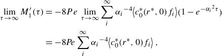 \begin{align} \lim _{\tau \rightarrow \infty }M_{1}^{\prime}(\tau )&=-8P\hspace{0pt}e\,\lim _{\tau \rightarrow \infty }\sum _{i}^{\infty }{\alpha _{i}}^{-4}\!\left\langle c _{0}^{*}(r^{*},0)f_{i}\right\rangle \!\big(1-e^{-{{\alpha _{i}}^{2}}\tau }\big)\nonumber\\&=-8\textit{Pe}\sum _{i}^{\infty }{\alpha _{i}}^{-4}\!\left\langle c _{0}^{*}(r^{*},0)f_{i}\right\rangle, \end{align}
and
 \begin{equation} \lim _{\tau \rightarrow \infty }M_{1}^{\prime}(\tau )=-16P\hspace{0pt}e\underset{\tau \rightarrow \infty }{\enspace \lim }\sum _{i}^{\infty }{\alpha _{i}}^{-4}\frac{1}{J_{0}\!\left(\alpha _{i}\right)}\!\Big(1-e^{-{{\alpha _{i}}^{2}}\tau }\Big)=-16\textit{Pe}\sum _{i}^{\infty }{\alpha _{i}}^{-4}\frac{1}{J_{0}\!\left(\alpha _{i}\right)} .\end{equation}
Equations (4.11) and (4.12) agree with Aris’ (Reference Aris1956) solution for the mean axial location of the solute. Specifically, (4.11) is equivalent to Aris’ (21) and (4.12) is equivalent to Aris’ (32) for an initial delta distribution of solute at $r^{*}=0$
.
$r^{*}=0$
.
Now that we have a solution for the first moment of solute, we can proceed with the separation of variables solution to ‘build up’ our solution for the second moment of solute, as previously mentioned. Accordingly, Barton (Reference Barton1983) further showed that the second moment of the solute distribution about the axial mean (again, for arbitrary geometries and velocity fields) behaves as follows:
 \begin{equation} v_{2}(\tau )=M_{2}-\left(M_{1}\right)^{2}=v_{2}\!\left(0\right)+2\left(1+\sum _{i}^{\infty }\frac{\left\langle \chi f_{i}\right\rangle ^{2}}{\mu _{i}}\right)\tau -2\sum _{i}^{\infty }\!\left\langle \chi f_{i}\right\rangle ^{2}\!\left(\frac{1-e^{-{\mu _{i}}\tau }}{{\mu _{i}}^{2}}\right) .\end{equation}
For the current work, $\langle \chi f_{i}\rangle$
and
$\langle \chi f_{i}\rangle$
and $\mu _{i}$
are given by (4.8) and (4.6), respectively. Equation (4.13) applies to solute that is initially distributed uniformly across the cross-section of the tube. Useful in comparing our MoM and quasi-steady formulations, we also define the transient effective dispersion coefficient to be half the rate of change of variance
$\mu _{i}$
are given by (4.8) and (4.6), respectively. Equation (4.13) applies to solute that is initially distributed uniformly across the cross-section of the tube. Useful in comparing our MoM and quasi-steady formulations, we also define the transient effective dispersion coefficient to be half the rate of change of variance
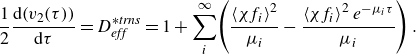 \begin{equation} \frac{1}{2}\frac{\mathrm{d}\!\left(v_{2}(\tau )\right)}{\mathrm{d}\tau }=D_{\textit{eff}}^{*\textit{trns}}=1+\sum _{i}^{\infty }\!\left(\frac{\left\langle \chi f_{i}\right\rangle ^{2}}{\mu _{i}}-\frac{\left\langle \chi f_{i}\right\rangle ^{2}e^{-{\mu _{i}}\tau }}{\mu _{i}}\right) .\end{equation}
(We note that Barton neither discusses this formulation nor makes this comparison.) Equation (4.14) provides the transient effective dispersion coefficient as a function of four dimensionless parameters ( $\textit{Pe}_{p}, \textit{Pe}_{e}, \tau$
and
$\textit{Pe}_{p}, \textit{Pe}_{e}, \tau$
and $\phi$
), and is also useful to the case of perfectly opposed EOF and PDF. However, because (4.14) is a function of four parameters, it is difficult to present clear visualisations of different regimes of the solution. To remedy this, we will again formulate the dispersion coefficient in terms of the parameter
$\phi$
), and is also useful to the case of perfectly opposed EOF and PDF. However, because (4.14) is a function of four parameters, it is difficult to present clear visualisations of different regimes of the solution. To remedy this, we will again formulate the dispersion coefficient in terms of the parameter $\beta$
and a Péclet number based on the sum of the EOF and PDF bulk velocities,
$\beta$
and a Péclet number based on the sum of the EOF and PDF bulk velocities, $\textit{Pe}=(\langle u_{p}\rangle +\langle u_{e}\rangle )a/D$
. Then, letting
$\textit{Pe}=(\langle u_{p}\rangle +\langle u_{e}\rangle )a/D$
. Then, letting $\hat{u}(r^{*})=u(r^{*})/\langle u\rangle$
, we write
$\hat{u}(r^{*})=u(r^{*})/\langle u\rangle$
, we write
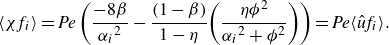 \begin{equation} \left\langle \chi f_{i}\right\rangle =\textit{Pe}\left(\frac{-8\beta }{{\alpha _{i}}^{2}}-\frac{(1-\beta)}{1-\eta }\!\left(\frac{\eta \phi ^{2}}{{\alpha _{i}}^{2}+\phi ^{2}}\right)\right)=\textit{Pe} \langle \hat{u}\!f_{i}\rangle .\end{equation}
Substituting (4.15) into (4.14), we may now again define a bulk Péclet-independent dispersion parameter as
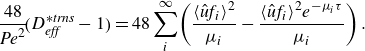 \begin{equation} \frac{48}{\textit{Pe}^{2}}\!\big(D_{\textit{eff}}^{*\textit{trns}}-1\big)=48\sum _{i}^{\infty }\!\left(\frac{\langle \hat{u}\!f_{i} \rangle ^{2}}{\mu _{i}}-\frac{ \langle \hat{u}\!f_{i} \rangle ^{2}e^{-{\mu _{i}}\tau }}{\mu _{i}}\right) .\end{equation}
The right-hand side of (4.16) is a function only of the dimensionless parameters $\beta, \phi$
and
$\beta, \phi$
and $\tau$
. This makes it easier to visualise than (4.14). We use the effective dispersion coefficient provided by (4.16) in most subsequent figures. Further, (4.16) asymptotes to our quasi-steady solution of the normalised dispersion coefficient (given by (3.21)) as
$\tau$
. This makes it easier to visualise than (4.14). We use the effective dispersion coefficient provided by (4.16) in most subsequent figures. Further, (4.16) asymptotes to our quasi-steady solution of the normalised dispersion coefficient (given by (3.21)) as $\tau \rightarrow \infty$
(we will note this in the discussion of figure 11).
$\tau \rightarrow \infty$
(we will note this in the discussion of figure 11).
Benchmark comparisons between Brownian dynamics simulations and the analytical solution of the early, transient growth of the effective dispersion coefficient normalised as $48\textit{Pe}^{-2}(D_{\textit{eff}}^{*\textit{trns}}-1)$
(non-solid curves) versus dimensionless time,
$48\textit{Pe}^{-2}(D_{\textit{eff}}^{*\textit{trns}}-1)$
(non-solid curves) versus dimensionless time, $\tau =\textit{tD}/a^{2}$
. The non-solid curves show the analytical solutions as derived from the MoM. The open markers show Brownian dynamics simulations benchmarking of the solutions. Curves in
$\tau =\textit{tD}/a^{2}$
. The non-solid curves show the analytical solutions as derived from the MoM. The open markers show Brownian dynamics simulations benchmarking of the solutions. Curves in $(a)$
are indexed by varying values of the tube radius scaled by Debye length,
$(a)$
are indexed by varying values of the tube radius scaled by Debye length, $\phi$
. Curves in
$\phi$
. Curves in $(b)$
are indexed by varying values of the fraction of bulk velocity caused by pressure,
$(b)$
are indexed by varying values of the fraction of bulk velocity caused by pressure, $\beta$
. The translucent horizontal line segments denote the analytical, quasi-steady state solutions.
$\beta$
. The translucent horizontal line segments denote the analytical, quasi-steady state solutions.
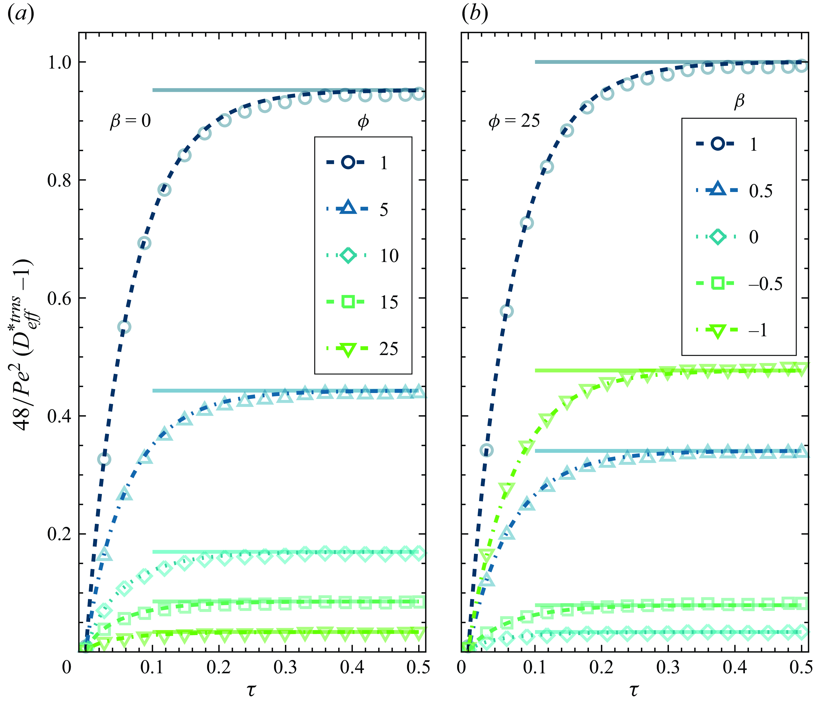
We note that for the special case of pure PDF ( $\textit{Pe}_{p}=\textit{Pe}$
), (4.13) reduces to Barton’s (Reference Barton1983) solution for the variance of solute in a cylindrical tube (Barton’s equation (5.4)). Further, again for pure PDF, (4.14) analytically reduces to Taghizadeh et al.’s (Reference Taghizadeh, Valdés-Parada and Wood2020) solution for the transient effective dispersion coefficient (Taghizadeh et al.’s equation (7.3)). Taghizadeh et al. analysed the dispersion of solute subject to purely PDF in a cylindrical tube across all time regimes. They applied a cross-sectional-averaging method and derived an analytical expression for the aforementioned transient effective dispersion coefficient, as well as an associated one-dimensional convection–diffusion equation (Taghizadeh et al.’s equation (6.6)). To find solutions to this area-averaged convection–diffusion equation, Taghizadeh et al. relied on a (numerical) finite element method. Lastly, for
$\textit{Pe}_{p}=\textit{Pe}$
), (4.13) reduces to Barton’s (Reference Barton1983) solution for the variance of solute in a cylindrical tube (Barton’s equation (5.4)). Further, again for pure PDF, (4.14) analytically reduces to Taghizadeh et al.’s (Reference Taghizadeh, Valdés-Parada and Wood2020) solution for the transient effective dispersion coefficient (Taghizadeh et al.’s equation (7.3)). Taghizadeh et al. analysed the dispersion of solute subject to purely PDF in a cylindrical tube across all time regimes. They applied a cross-sectional-averaging method and derived an analytical expression for the aforementioned transient effective dispersion coefficient, as well as an associated one-dimensional convection–diffusion equation (Taghizadeh et al.’s equation (6.6)). To find solutions to this area-averaged convection–diffusion equation, Taghizadeh et al. relied on a (numerical) finite element method. Lastly, for $\textit{Pe}_{p}=\textit{Pe}$
and in the limit as
$\textit{Pe}_{p}=\textit{Pe}$
and in the limit as $\tau \rightarrow \infty$
, (4.14) reduces to Aris’ (Reference Aris1956) solution for the steady effective dispersion coefficient (Aris’ equation (26)). Hence, our solutions for the solute variance and effective dispersion coefficient agree with and reduce to those of Aris (Reference Aris1956), Barton (Reference Barton1983) and Taghizadeh et al. (Reference Taghizadeh, Valdés-Parada and Wood2020) for the special case of pure PDF.
$\tau \rightarrow \infty$
, (4.14) reduces to Aris’ (Reference Aris1956) solution for the steady effective dispersion coefficient (Aris’ equation (26)). Hence, our solutions for the solute variance and effective dispersion coefficient agree with and reduce to those of Aris (Reference Aris1956), Barton (Reference Barton1983) and Taghizadeh et al. (Reference Taghizadeh, Valdés-Parada and Wood2020) for the special case of pure PDF.
Lastly, we offer a note regarding the second or third moments about the mean for the current velocity fields. For arbitrary initial conditions, such a solution requires the evaluation of the following integral:
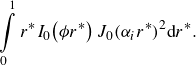 \begin{equation} \int\limits _{0}^{1}r^{*}I_{0}\!\left(\phi r^{*}\right)J_{0} (\alpha _{i}r^{*})^{2}\mathrm{d}r^{*} .\end{equation}
We know of no analytical solution to this integral.
4.1. Minimisation of variance for transporting solute over a fixed axial distance
We analytically explore the minimisation of variance for transporting solute over some fixed axial distance of interest. This treatment considers, for example, an engineering situation in a microfluidic device where a cloud of solute is transported a distance $L$
from one location in a microchannel to a second location over some characteristic time
$L$
from one location in a microchannel to a second location over some characteristic time $\tau _{o}$
. The following analysis allows the user of this device to maximise the area-averaged concentration of the arriving solute by minimising dispersion. Importantly, and in contrast to the optimisation in § 3.3, this analysis applies to values of the characteristic transport time
$\tau _{o}$
. The following analysis allows the user of this device to maximise the area-averaged concentration of the arriving solute by minimising dispersion. Importantly, and in contrast to the optimisation in § 3.3, this analysis applies to values of the characteristic transport time $\tau _{o}$
that are any duration relative to the characteristic time of transverse diffusion,
$\tau _{o}$
that are any duration relative to the characteristic time of transverse diffusion, $a^{2}/D$
. In particular, the following analysis is applicable to processes which are brief (in terms of
$a^{2}/D$
. In particular, the following analysis is applicable to processes which are brief (in terms of $\tau _{o}$
) compared with the transverse diffusion time. The fixed value of solute transport distance is here relevant (whereas the precise distance of transport was irrelevant in § 3.3). We are only interested in minimising variance for moving solute, so we preclude the case of
$\tau _{o}$
) compared with the transverse diffusion time. The fixed value of solute transport distance is here relevant (whereas the precise distance of transport was irrelevant in § 3.3). We are only interested in minimising variance for moving solute, so we preclude the case of $\langle u\rangle \approx 0$
. First, if
$\langle u\rangle \approx 0$
. First, if $\phi$
may be varied, then it should be made as large as possible to help minimise variance (as mentioned in § 3.3). However, we henceforth assume
$\phi$
may be varied, then it should be made as large as possible to help minimise variance (as mentioned in § 3.3). However, we henceforth assume $\phi$
to be finite and fixed. Because we assumed
$\phi$
to be finite and fixed. Because we assumed $\langle u\rangle \neq 0$
, it is convenient to optimise the velocity profile in terms of the parameters
$\langle u\rangle \neq 0$
, it is convenient to optimise the velocity profile in terms of the parameters $\beta =\langle u_{p}\rangle /\langle u\rangle$
and
$\beta =\langle u_{p}\rangle /\langle u\rangle$
and $\textit{Pe}$
. Substituting (4.15) into (4.13), we first present the variance of the solute zone in terms of these parameters
$\textit{Pe}$
. Substituting (4.15) into (4.13), we first present the variance of the solute zone in terms of these parameters
 \begin{equation} v_{2}(\tau )=v_{2}\!\left(0\right)+2\left(1+\textit{Pe}^{2}\sum _{i}^{\infty }\frac{ \langle \hat{u}f_{i} \rangle ^{2}}{\mu _{i}}\right)\tau -2\textit{Pe}^{2}\sum _{i}^{\infty } \langle \hat{u}f_{i}\rangle ^{2}\!\left(\frac{1-e^{-{\mu _{i}}\tau }}{{\mu _{i}}^{2}}\right) .\end{equation}
Given this formulation, we will show that the value of $\beta$
required to minimise variance for transporting solute over a fixed distance (henceforth denoted
$\beta$
required to minimise variance for transporting solute over a fixed distance (henceforth denoted $\beta _{o}^{\textit{trns}}(\tau _{o})$
) depends only on the characteristic dimensionless time to transport solute over that given distance,
$\beta _{o}^{\textit{trns}}(\tau _{o})$
) depends only on the characteristic dimensionless time to transport solute over that given distance, $\tau _{o}$
, and the dimensionless parameter
$\tau _{o}$
, and the dimensionless parameter $\phi$
. Now, we solved the steady Stokes equation for our velocity profile. Hence, upon injection of solute into the tube, all parameters related to the velocity field (e.g.
$\phi$
. Now, we solved the steady Stokes equation for our velocity profile. Hence, upon injection of solute into the tube, all parameters related to the velocity field (e.g. $\beta, \phi$
and
$\beta, \phi$
and $\textit{Pe}$
) are immediately ‘set’ and cannot vary with time. For the minimisation, we differentiate (4.18) with respect to
$\textit{Pe}$
) are immediately ‘set’ and cannot vary with time. For the minimisation, we differentiate (4.18) with respect to $\beta$
, substitute
$\beta$
, substitute $\tau =\tau _{o}$
, and then set the resulting quantity equal to zero
$\tau =\tau _{o}$
, and then set the resulting quantity equal to zero
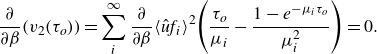 \begin{equation} \frac{\partial }{\partial \beta }\!\left(v_{2}\!\left(\tau _{o}\right)\right)=\sum _{i}^{\infty }\frac{\partial }{\partial \beta } \langle \hat{u}\!f_{i} \rangle ^{2}\!\left(\frac{\tau _{o}}{\mu _{i}}-\frac{1-e^{-{\mu _{i}}{\tau _{o}}}}{\mu _{i}^{2}}\right)=0 .\end{equation}
The only value dependent on $\beta$
in (4.19) is
$\beta$
in (4.19) is $\langle \hat{u}f_{i}\rangle ^{2}$
, so we evaluate as follows:
$\langle \hat{u}f_{i}\rangle ^{2}$
, so we evaluate as follows:
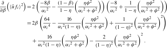 \begin{align} \frac{\partial }{\partial \beta }\!\left(\langle \hat{u}f_{i} \rangle ^{2}\right)&=2\left(\frac{-8\beta }{{\alpha _{i}}^{2}}-\frac{(1-\beta)}{1-\eta }\!\left(\frac{\eta \phi ^{2}}{{\alpha _{i}}^{2}+\phi ^{2}}\right)\right)\left(\frac{-8}{{\alpha _{i}}^{2}}+\frac{1}{1-\eta }\!\left(\frac{\eta \phi ^{2}}{{\alpha _{i}}^{2}+\phi ^{2}}\right)\right)\nonumber\\&= 2\beta \left(\frac{64}{{\alpha _{i}}^{4}}-\frac{16}{{\alpha _{i}}^{2}\!\left(1-\eta \right)}\!\left(\frac{\eta \phi ^{2}}{{\alpha _{i}}^{2}+\phi ^{2}}\right)+\frac{1}{\left(1-\eta \right)^{2}}\!\left(\frac{\eta \phi ^{2}}{{\alpha _{i}}^{2}+\phi ^{2}}\right)^{2}\right)\nonumber\\&\quad +\frac{16}{{\alpha _{i}}^{2}\!\left(1-\eta \right)}\!\left(\frac{\eta \phi ^{2}}{{\alpha _{i}}^{2}+\phi ^{2}}\right)-\frac{2}{\left(1-\eta \right)^{2}}\!\left(\frac{\eta \phi ^{2}}{{\alpha _{i}}^{2}+\phi ^{2}}\right)^{2}. \end{align}
We substitute (4.20) into (4.19) and rearrange to find
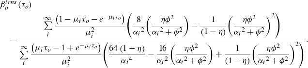 \begin{align} & \beta^{trns}_{o}(\tau_{o}) \nonumber \\& \quad =\frac{\sum\limits _{i}^{\infty }\dfrac{\left(1-\mu _{i}\tau _{o}-e^{-{\mu _{i}}{\tau _{o}}}\right)}{\mu _{i}^{2}}\!\left(\dfrac{8}{{\alpha _{i}}^{2}}\!\left(\dfrac{\eta \phi ^{2}}{{\alpha _{i}}^{2}+\phi ^{2}}\right)-\dfrac{1}{\left(1-\eta \right)}\!\left(\dfrac{\eta \phi ^{2}}{{\alpha _{i}}^{2}+\phi ^{2}}\right)^{2}\right)}{\sum\limits _{i}^{\infty }\dfrac{\left(\mu _{i}\tau _{o}-1+e^{-{\mu _{i}}{\tau _{o}}}\right)}{\mu _{i}^{2}}\!\left(\dfrac{64\left(1-\eta \right)}{{\alpha _{i}}^{4}}-\dfrac{16}{{\alpha _{i}}^{2}}\!\left(\dfrac{\eta \phi ^{2}}{{\alpha _{i}}^{2}+\phi ^{2}}\right)+\dfrac{1}{\left(1-\eta \right)}\!\left(\dfrac{\eta \phi ^{2}}{{\alpha _{i}}^{2}+\phi ^{2}}\right)^{2}\right)} .\end{align}
The latter expression provides the unique value of $\beta$
that minimises the dispersion across all time regimes. Equation (4.21) depends only on
$\beta$
that minimises the dispersion across all time regimes. Equation (4.21) depends only on $\tau _{o}$
and
$\tau _{o}$
and $\phi$
. For example, if we specify the value of
$\phi$
. For example, if we specify the value of $\tau _{o}$
as the characteristic time to transport solute through a tube, then (4.21) can be used to find the fixed value of
$\tau _{o}$
as the characteristic time to transport solute through a tube, then (4.21) can be used to find the fixed value of $\beta _{o}^{\textit{trns}}(\tau _{o})$
that minimises variance for such transport. We note that (4.21) asymptotes to
$\beta _{o}^{\textit{trns}}(\tau _{o})$
that minimises variance for such transport. We note that (4.21) asymptotes to $\beta _{o}$
of our quasi-steady solution as
$\beta _{o}$
of our quasi-steady solution as $\tau _{o}\rightarrow \infty$
(see figure 12).
$\tau _{o}\rightarrow \infty$
(see figure 12).
Deviation of the transient value of the variance-minimising fraction of bulk velocity caused by pressure, $\beta _{o}^{\textit{trns}}(\tau _{o})$
, from the quasi-steady state value,
$\beta _{o}^{\textit{trns}}(\tau _{o})$
, from the quasi-steady state value, $\beta _{o}$
, versus the characteristic dimensionless time of interest,
$\beta _{o}$
, versus the characteristic dimensionless time of interest, $\tau _{o}$
. The curves are indexed by the tube radius scaled by Debye length,
$\tau _{o}$
. The curves are indexed by the tube radius scaled by Debye length, $\phi$
. The inset is a closeup for the interval of
$\phi$
. The inset is a closeup for the interval of $0\lt \tau _{o}\lt 0.1$
. Dispersion caused by predominantly EOF with very thin EDLs (e.g.
$0\lt \tau _{o}\lt 0.1$
. Dispersion caused by predominantly EOF with very thin EDLs (e.g. $\phi \gt 50$
) very quickly asymptotes to quasi-steady state dynamics.
$\phi \gt 50$
) very quickly asymptotes to quasi-steady state dynamics.
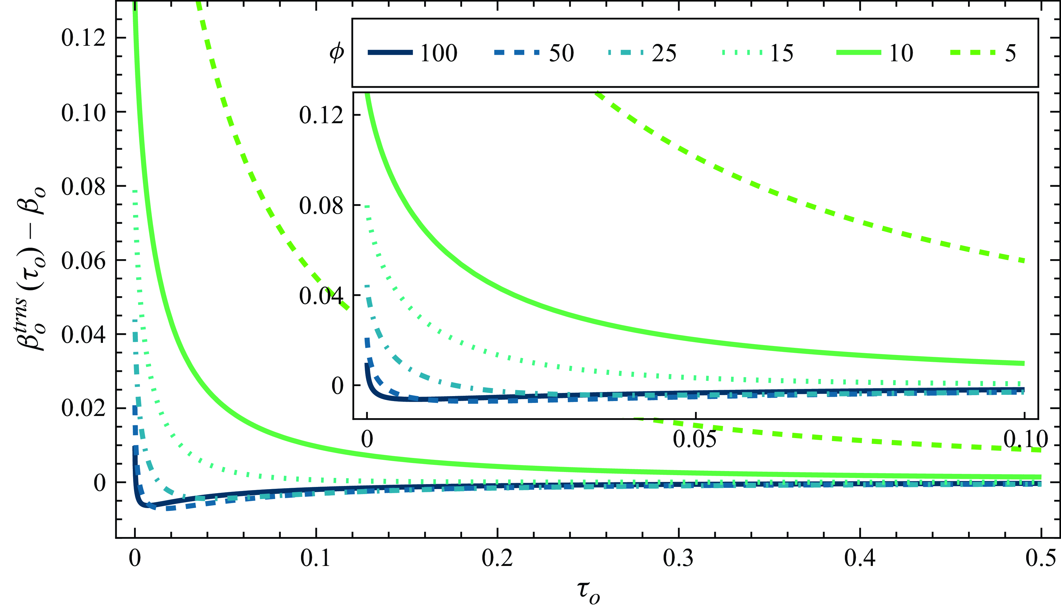
Next, we are also interested in deriving the optimum Péclet number $P\hspace{0pt}e_{o}^{\textit{trns}}$
to minimise the variance for transporting the solute over some fixed dimensionless axial distance of interest,
$P\hspace{0pt}e_{o}^{\textit{trns}}$
to minimise the variance for transporting the solute over some fixed dimensionless axial distance of interest, $L^{*}$
. To this end, we substitute
$L^{*}$
. To this end, we substitute $\tau =L^{*}/\textit{Pe}$
into (4.18), then set the derivative with respect to
$\tau =L^{*}/\textit{Pe}$
into (4.18), then set the derivative with respect to $P\hspace{0pt}e$
equal to zero
$P\hspace{0pt}e$
equal to zero
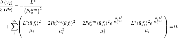 \begin{align} &\frac{\partial \left(v_{2}\right)}{\partial \left(\textit{Pe}\right)}=-\frac{L^{*}}{\left(\textit{Pe}_{o}^{\textit{trns}}\right)^{2}}\nonumber\\&\quad+\sum _{i}^{\infty }\!\left(\frac{L^{*}\!\langle \hat{u}f_{i}\rangle ^{2}}{\mu _{i}}-\frac{2\textit{Pe}_{o}^{\textit{trns}} \langle \hat{u}f_{i}\rangle ^{2}}{\mu _{i}^{2}}+\frac{2\textit{Pe}_{o}^{\textit{trns}} \langle \hat{u}f_{i}\rangle ^{2}e^{\frac{-\mu _{i}L^{*}}{\textit{Pe}_{o}^{\textit{trns}}}}}{\mu _{i}^{2}}+\frac{L^{*} \langle \hat{u}f_{i}\rangle ^{2}e^{\frac{-\mu _{i}L^{*}}{\textit{Pe}_{o}^{\textit{trns}}}}}{\mu _{i}}\right)=0 .\end{align}
Multiplying by $(P\hspace{0pt}e_{o}^{\textit{trns}})^{2}$
and rearranging, (4.22) can be expressed as
$(P\hspace{0pt}e_{o}^{\textit{trns}})^{2}$
and rearranging, (4.22) can be expressed as
 \begin{equation} -L^{*}+\sum _{i}^{\infty }\!\left(\!L^{*}\!\left(P\hspace{0pt}e_{o}^{\textit{trns}}\right)^{2}\frac{\langle \hat{u}f_{i}\rangle ^{2}}{\mu _{i}}\!\left(\!1+e^{\frac{-\mu _{i}L^{*}}{\textit{Pe}_{o}^{\textit{trns}}}}\right)+2\left(P\hspace{0pt}e_{o}^{\textit{trns}}\right)^{3}\frac{ \langle \hat{u}f_{i}\rangle ^{2}}{\mu _{i}^{2}}\!\left(e^{\frac{-\mu _{i}L^{*}}{\textit{Pe}_{o}^{\textit{trns}}}}-1\right)\!\right)=0 .\end{equation}
We will now explain the process to find the optimum combination of $\beta$
and
$\beta$
and $\textit{Pe}$
to minimise variance for transporting solute over a fixed axial distance (again assuming
$\textit{Pe}$
to minimise variance for transporting solute over a fixed axial distance (again assuming $\phi$
to be fixed). Recall from (4.15) that
$\phi$
to be fixed). Recall from (4.15) that $\langle \hat{u}f_{i}\rangle$
and therefore (4.23) are functions of
$\langle \hat{u}f_{i}\rangle$
and therefore (4.23) are functions of $\beta$
. Thus, to find the global optimum value of
$\beta$
. Thus, to find the global optimum value of $P\hspace{0pt}e_{o}^{\textit{trns}}$
for a fixed value of
$P\hspace{0pt}e_{o}^{\textit{trns}}$
for a fixed value of $L^{*}$
, we first substitute the
$L^{*}$
, we first substitute the $\beta _{o}^{\textit{trns}}(\tau _{o})$
function as given by (4.21) into (4.23). We then substitute
$\beta _{o}^{\textit{trns}}(\tau _{o})$
function as given by (4.21) into (4.23). We then substitute $\tau _{o}=L^{*}/P\hspace{0pt}e_{o}^{\textit{trns}}$
into (4.23). Next, we solve the resulting equation for
$\tau _{o}=L^{*}/P\hspace{0pt}e_{o}^{\textit{trns}}$
into (4.23). Next, we solve the resulting equation for $P\hspace{0pt}e_{o}^{\textit{trns}}$
using the Newton–Raphson method (Engquist Reference Engquist2015, pp. 1023–1028) or some other root-finding method. Once we have
$P\hspace{0pt}e_{o}^{\textit{trns}}$
using the Newton–Raphson method (Engquist Reference Engquist2015, pp. 1023–1028) or some other root-finding method. Once we have $P\hspace{0pt}e_{o}^{\textit{trns}}$
for a given value of
$P\hspace{0pt}e_{o}^{\textit{trns}}$
for a given value of $L^{*}$
, we can again use the relationship
$L^{*}$
, we can again use the relationship $\tau _{o}=L^{*}/P\hspace{0pt}e_{o}^{\textit{trns}}$
to find the corresponding value of
$\tau _{o}=L^{*}/P\hspace{0pt}e_{o}^{\textit{trns}}$
to find the corresponding value of $\tau _{o}$
. Next, using (4.21), we compute the specific value of
$\tau _{o}$
. Next, using (4.21), we compute the specific value of $\beta _{o}^{\textit{trns}}(\tau _{o})$
at that value of
$\beta _{o}^{\textit{trns}}(\tau _{o})$
at that value of $\tau _{o}$
. Thus, this process gives the fixed global optimum values of
$\tau _{o}$
. Thus, this process gives the fixed global optimum values of $\textit{Pe}$
and
$\textit{Pe}$
and $\beta$
to minimise variance for transporting solute over a dimensionless distance
$\beta$
to minimise variance for transporting solute over a dimensionless distance $L^{*}$
. Lastly, per figure 13, we note that
$L^{*}$
. Lastly, per figure 13, we note that $P\hspace{0pt}e_{o}^{\textit{trns}}$
asymptotes to
$P\hspace{0pt}e_{o}^{\textit{trns}}$
asymptotes to $\textit{Pe}_{o}$
as
$\textit{Pe}_{o}$
as $L^{*}\rightarrow \infty$
.
$L^{*}\rightarrow \infty$
.
Solutions related to the transient variance-minimising Péclet number, $\textit{Pe}_{o}^{\textit{trns}}$
. In
$\textit{Pe}_{o}^{\textit{trns}}$
. In $(a), \textit{Pe}_{o}^{\textit{trns}}$
is plotted as a function of the dimensionless axial distance of travel,
$(a), \textit{Pe}_{o}^{\textit{trns}}$
is plotted as a function of the dimensionless axial distance of travel, $L^{*}$
. The non-solid curves indicate transient solutions from the MoM. The translucent horizontal line segments denote the associated quasi-steady state solutions. The quasi-steady and transient solutions agree asymptotically after approximately
$L^{*}$
. The non-solid curves indicate transient solutions from the MoM. The translucent horizontal line segments denote the associated quasi-steady state solutions. The quasi-steady and transient solutions agree asymptotically after approximately $L^{*}=100$
.
$L^{*}=100$
. $(b)$
Variance,
$(b)$
Variance, $v_{2}(\tau _{o}=L^{*}/\textit{Pe})$
, of the solute zone after travelling a dimensionless axial distance of
$v_{2}(\tau _{o}=L^{*}/\textit{Pe})$
, of the solute zone after travelling a dimensionless axial distance of $L^{*}=100$
as a function of Péclet number,
$L^{*}=100$
as a function of Péclet number, $P\hspace{0pt}e$
. The red dots indicate minima of
$P\hspace{0pt}e$
. The red dots indicate minima of $v_{2}(\tau _{o})$
as determined from the solution of
$v_{2}(\tau _{o})$
as determined from the solution of $\textit{Pe}_{o}^{\textit{trns}}$
from (4.23). For both panels, curves are indexed by the tube radius scaled by Debye length,
$\textit{Pe}_{o}^{\textit{trns}}$
from (4.23). For both panels, curves are indexed by the tube radius scaled by Debye length, $\phi$
. Figure 13 was produced by setting
$\phi$
. Figure 13 was produced by setting $\tau _{o}=L^{*}/\textit{Pe}$
and
$\tau _{o}=L^{*}/\textit{Pe}$
and $\beta =\beta _{o}^{\textit{trns}}(\tau _{o})$
.
$\beta =\beta _{o}^{\textit{trns}}(\tau _{o})$
.
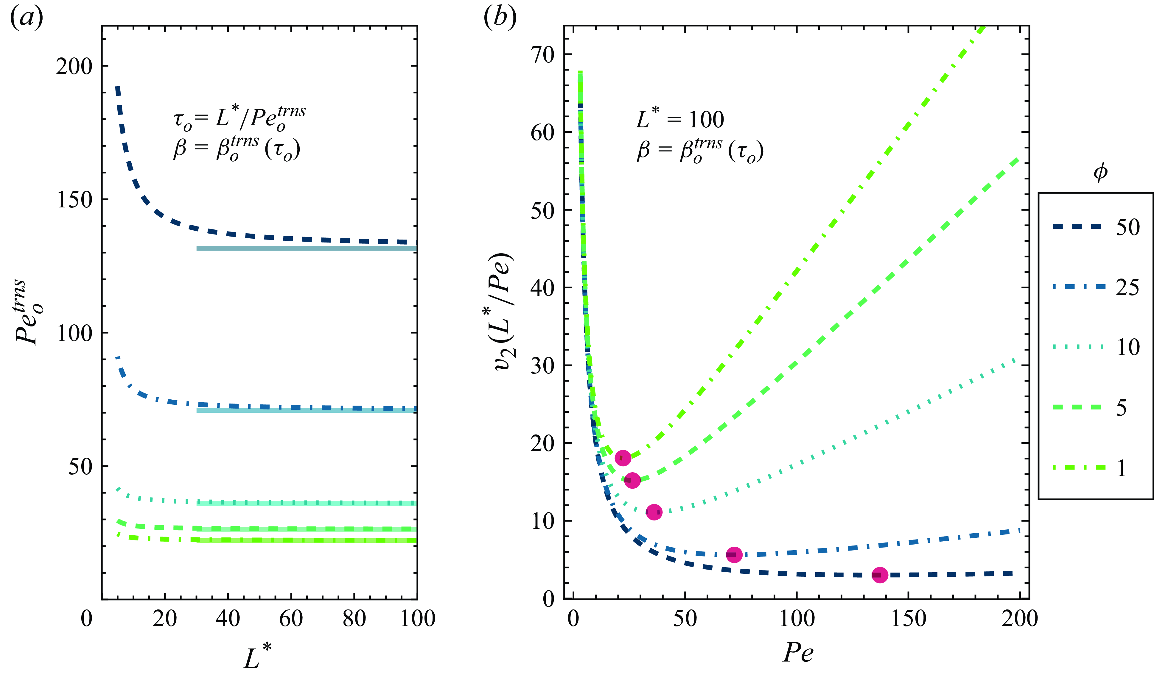
5. Results and discussion
We first visualise our analytical solution for the concentration field given a ‘top hat’ initial condition (equation (3.40)). Figure 3 shows solute concentration profiles, determined from the quasi-steady solution. Each curve shows the normalised solute concentration, $c^{*}(x^{\prime*}|r^{*},\tau )=\pi a^{3}c(x^{\prime*}|r^{*},\tau )/N$
, on the ordinate. The abscissa is a dimensionless axial position in a frame moving at solute bulk velocity,
$c^{*}(x^{\prime*}|r^{*},\tau )=\pi a^{3}c(x^{\prime*}|r^{*},\tau )/N$
, on the ordinate. The abscissa is a dimensionless axial position in a frame moving at solute bulk velocity, $x^{\prime*}=x^{*}-\tau P\hspace{0pt}e$
. These curves are axial profiles from the two-dimensional unsteady solution at select radial coordinates and select times as indicated in the figure. Profiles are shown for four combinations of
$x^{\prime*}=x^{*}-\tau P\hspace{0pt}e$
. These curves are axial profiles from the two-dimensional unsteady solution at select radial coordinates and select times as indicated in the figure. Profiles are shown for four combinations of $\textit{Pe}_{e}, \textit{Pe}_{p}$
and
$\textit{Pe}_{e}, \textit{Pe}_{p}$
and $\phi$
, corresponding to the four figure panels. Each individual panel shows solute concentration profiles at three distinct values of dimensionless time (different line colours) for three separate radial positions (different line types), resulting in nine solute profiles per panel. EOF with thin EDLs results in very little solute dispersion and thus exhibits the highest solute concentrations. In contrast, EOF with relatively thick EDLs or PDF causes the solute to disperse quickly. Additionally, the radial deviation of solute is relatively small for all values of
$\phi$
, corresponding to the four figure panels. Each individual panel shows solute concentration profiles at three distinct values of dimensionless time (different line colours) for three separate radial positions (different line types), resulting in nine solute profiles per panel. EOF with thin EDLs results in very little solute dispersion and thus exhibits the highest solute concentrations. In contrast, EOF with relatively thick EDLs or PDF causes the solute to disperse quickly. Additionally, the radial deviation of solute is relatively small for all values of $\tau$
shown, but easily observable for
$\tau$
shown, but easily observable for $\tau \leq 5$
.
$\tau \leq 5$
.
We next compare our expression for the concentration field resulting from a ‘top hat’ initial condition (cf. (3.40)) with Brownian dynamics simulations to benchmark our analytical model. Figure 4 shows comparisons for the temporal evolution of the solute concentration field at an example bulk Péclet number of 100. The radius of the tube has been enlarged relative to the axial length for clarity of presentation. The three columns (solute shown in blue, orange and green) correspond to values of dimensionless time, $\tau =\textit{tD}/a^{2}$
, of 2.5, 100 and 400, respectively. The dimensionless radius,
$\tau =\textit{tD}/a^{2}$
, of 2.5, 100 and 400, respectively. The dimensionless radius, $r^{*}$
, is on the ordinate and dimensionless axial position,
$r^{*}$
, is on the ordinate and dimensionless axial position, $x^{*}$
, is on the abscissa. The four rows are plots for example values of
$x^{*}$
, is on the abscissa. The four rows are plots for example values of $P\hspace{0pt}e_{p}, P\hspace{0pt}e_{e}$
and
$P\hspace{0pt}e_{p}, P\hspace{0pt}e_{e}$
and $\phi$
, consistent with various combinations of EOF and PDF. The analytical solution and Brownian dynamics simulations show excellent agreement for all combinations of parameters. This figure shows the full, two-dimensional concentration field, including the radial distribution of solute particles for both the Brownian dynamics simulations and the solute stream (cf. (3.11)). The radial variation of solute for this Péclet number is very slight. Figure 4 was made with a value of
$\phi$
, consistent with various combinations of EOF and PDF. The analytical solution and Brownian dynamics simulations show excellent agreement for all combinations of parameters. This figure shows the full, two-dimensional concentration field, including the radial distribution of solute particles for both the Brownian dynamics simulations and the solute stream (cf. (3.11)). The radial variation of solute for this Péclet number is very slight. Figure 4 was made with a value of $\textit{Pe}=100$
; we provide similar figures for values of
$\textit{Pe}=100$
; we provide similar figures for values of $\textit{Pe}=$
20 and 1000 in § B of the SM.
$\textit{Pe}=$
20 and 1000 in § B of the SM.
As per (3.19), for $\textit{Pe}_{p}$
and
$\textit{Pe}_{p}$
and $\textit{Pe}_{e}$
both greater than or equal to zero, the rate of growth of the variance decreases as
$\textit{Pe}_{e}$
both greater than or equal to zero, the rate of growth of the variance decreases as $\phi$
increases or
$\phi$
increases or $\textit{Pe}_{p}/\textit{Pe}_{e}$
decreases. That is, for EOF and PDF in the same direction, variance growth is smaller for thinner EDLs and/or larger relative amounts of EOF compared to PDF.
$\textit{Pe}_{p}/\textit{Pe}_{e}$
decreases. That is, for EOF and PDF in the same direction, variance growth is smaller for thinner EDLs and/or larger relative amounts of EOF compared to PDF.
Figure 5 shows comparisons between Brownian dynamics simulations and the analytical solution of the temporal evolution of solute for the specific case where EOF is perfectly opposed by PDF (resulting in a flow with zero area-averaged bulk velocity). The plot was constructed with example values of $\textit{Pe}_{e}=100, \textit{Pe}_{p}=-100$
and four values of
$\textit{Pe}_{e}=100, \textit{Pe}_{p}=-100$
and four values of $\phi$
(corresponding to the four rows). Dimensionless radius,
$\phi$
(corresponding to the four rows). Dimensionless radius, $r^{*}$
, is shown on the ordinate and dimensionless axial position,
$r^{*}$
, is shown on the ordinate and dimensionless axial position, $x^{*}$
, is on the abscissa. The three columns (solute clouds in blue, orange and green) correspond to values of dimensionless time,
$x^{*}$
, is on the abscissa. The three columns (solute clouds in blue, orange and green) correspond to values of dimensionless time, $\tau$
, of 5.0, 100 and 400, respectively. The analytical solution and Brownian dynamics simulations show excellent agreement for all combinations of parameters.
$\tau$
, of 5.0, 100 and 400, respectively. The analytical solution and Brownian dynamics simulations show excellent agreement for all combinations of parameters.
Figure 6 shows comparisons between the analytical solution (cf. (3.40)) and Brownian dynamics simulations of the temporal development of the normalised radial distribution of solute, $c^{\prime}(r^{*},x^{*},\tau )/\langle c\rangle (x^{*}=\tau \textit{Pe},\tau )=c^{\prime}(\langle c\rangle | _{x^{*}=\tau \textit{Pe}})^{-1}$
. Here,
$c^{\prime}(r^{*},x^{*},\tau )/\langle c\rangle (x^{*}=\tau \textit{Pe},\tau )=c^{\prime}(\langle c\rangle | _{x^{*}=\tau \textit{Pe}})^{-1}$
. Here, $\langle c\rangle (x^{*}=\tau \textit{Pe},\tau )$
is the area-averaged concentration at the mean axial position of solute. For figure 6, we chose an example Péclet number of 100. For the Brownian dynamics, we considered the average results of 3000 separate simulation realisations with random seed initial conditions. In each realisation, we tracked 5000 particles initially arranged in a disk and distributed uniformly across the channel cross-section. The three columns correspond to values of dimensionless time,
$\langle c\rangle (x^{*}=\tau \textit{Pe},\tau )$
is the area-averaged concentration at the mean axial position of solute. For figure 6, we chose an example Péclet number of 100. For the Brownian dynamics, we considered the average results of 3000 separate simulation realisations with random seed initial conditions. In each realisation, we tracked 5000 particles initially arranged in a disk and distributed uniformly across the channel cross-section. The three columns correspond to values of dimensionless time, $\tau$
, of 1.5, 3.0 and 4.0. The dimensionless radius,
$\tau$
, of 1.5, 3.0 and 4.0. The dimensionless radius, $r^{*}$
, is on the ordinate and dimensionless axial position,
$r^{*}$
, is on the ordinate and dimensionless axial position, $x^{*}$
, is on the abscissa. The range of
$x^{*}$
, is on the abscissa. The range of $x^{*}$
is the same within each column. The dotted black lines denote two standard deviations of the Brownian particles’ axial positions about their mean position. The four rows correspond to the four values of
$x^{*}$
is the same within each column. The dotted black lines denote two standard deviations of the Brownian particles’ axial positions about their mean position. The four rows correspond to the four values of $\beta$
and
$\beta$
and $\phi$
shown (parameters equivalent to the four rows of figure 4). As before, Brownian dynamics simulations are plotted in the top half of each channel, and the Taylor-type solution on the bottom. To aid comparison, the number densities estimated from the Brownian simulations were smoothed via cubic interpolation to generate a scalar surface that minimises the net curvature of the simulation data. The analytical solution shows very good agreement with Brownian dynamics simulations for all choices of flow parameters. At the mean axial position of the solute (
$\phi$
shown (parameters equivalent to the four rows of figure 4). As before, Brownian dynamics simulations are plotted in the top half of each channel, and the Taylor-type solution on the bottom. To aid comparison, the number densities estimated from the Brownian simulations were smoothed via cubic interpolation to generate a scalar surface that minimises the net curvature of the simulation data. The analytical solution shows very good agreement with Brownian dynamics simulations for all choices of flow parameters. At the mean axial position of the solute ( $x^{*}=\tau \textit{Pe}$
),
$x^{*}=\tau \textit{Pe}$
), $c^{\prime}$
is identically zero across the entire channel cross-section. As the quantity
$c^{\prime}$
is identically zero across the entire channel cross-section. As the quantity $x^{*}-\tau \textit{Pe}$
grows large in magnitude,
$x^{*}-\tau \textit{Pe}$
grows large in magnitude, $c^{\prime}$
is a relatively small perturbation on the area-average concentration (and becomes smaller as
$c^{\prime}$
is a relatively small perturbation on the area-average concentration (and becomes smaller as $\tau$
increases). For example, at
$\tau$
increases). For example, at $\tau =4.0$
, the maximum observed magnitude of
$\tau =4.0$
, the maximum observed magnitude of $c^{\prime}(\langle c\rangle | _{x^{*}=\tau \textit{Pe}})^{-1}$
at the axial centreline was 0.12 (which we observed for pure PDF). By comparison, at
$c^{\prime}(\langle c\rangle | _{x^{*}=\tau \textit{Pe}})^{-1}$
at the axial centreline was 0.12 (which we observed for pure PDF). By comparison, at $\tau =10$
(not shown), the maximum value of
$\tau =10$
(not shown), the maximum value of $c^{\prime}(\langle c\rangle | _{x^{*}=\tau \textit{Pe}})^{-1}$
is 0.08. For
$c^{\prime}(\langle c\rangle | _{x^{*}=\tau \textit{Pe}})^{-1}$
is 0.08. For $\tau =100$
(not shown), this maximum magnitude of
$\tau =100$
(not shown), this maximum magnitude of $c^{\prime}(\langle c\rangle | _{x^{*}=\tau \textit{Pe}})^{-1}$
is 0.02. Lastly,
$c^{\prime}(\langle c\rangle | _{x^{*}=\tau \textit{Pe}})^{-1}$
is 0.02. Lastly, $c^{\prime}(\langle c\rangle | _{x^{*}=\tau \textit{Pe}})^{-1}$
approaches zero much faster (temporally) for thin-EDL EOF than for either PDF or thick-EDL EOF. We shall discuss this (and its effects on the characteristic time to reach quasi-steady dispersion dynamics) further when presenting figure 11.
$c^{\prime}(\langle c\rangle | _{x^{*}=\tau \textit{Pe}})^{-1}$
approaches zero much faster (temporally) for thin-EDL EOF than for either PDF or thick-EDL EOF. We shall discuss this (and its effects on the characteristic time to reach quasi-steady dispersion dynamics) further when presenting figure 11.
Next, figure 7 shows comparisons between the analytical solution (given by (3.21)) and Brownian dynamics simulations of the normalised effective dispersion coefficient, $48\textit{Pe}^{-2}(D_{\textit{eff}}^{*}-1)$
, as a function of
$48\textit{Pe}^{-2}(D_{\textit{eff}}^{*}-1)$
, as a function of $\beta$
and
$\beta$
and $\phi$
. The function
$\phi$
. The function $48\textit{Pe}^{-2}(D_{\textit{eff}}^{*}-1)$
reduces to unity when the effective dispersion coefficient approaches that of the classical Taylor dispersion for a simple parabolic flow profile. The analytical model shows excellent agreement with the Brownian dynamics simulations across the entire regime of flows. This includes both thin and thick (including overlapping) EDLs. The velocity fields evaluated in figure 7 include flows with PDF supporting EOF as well as PDF in opposition to EOF. The normalised dispersion coefficient
$48\textit{Pe}^{-2}(D_{\textit{eff}}^{*}-1)$
reduces to unity when the effective dispersion coefficient approaches that of the classical Taylor dispersion for a simple parabolic flow profile. The analytical model shows excellent agreement with the Brownian dynamics simulations across the entire regime of flows. This includes both thin and thick (including overlapping) EDLs. The velocity fields evaluated in figure 7 include flows with PDF supporting EOF as well as PDF in opposition to EOF. The normalised dispersion coefficient $48\textit{Pe}^{-2}(D_{\textit{eff}}^{*}-1)$
decreases as
$48\textit{Pe}^{-2}(D_{\textit{eff}}^{*}-1)$
decreases as $\phi$
increases (thinner EDLs) for values of
$\phi$
increases (thinner EDLs) for values of $0\leq \beta \leq 1$
, and tends to increase as
$0\leq \beta \leq 1$
, and tends to increase as $\phi$
increases for values of
$\phi$
increases for values of $\beta$
outside this interval. Interestingly, for values of
$\beta$
outside this interval. Interestingly, for values of $\beta$
near zero (EOF-dominated) and sufficiently thin EDLs,
$\beta$
near zero (EOF-dominated) and sufficiently thin EDLs, $48\textit{Pe}^{-2}(D_{\textit{eff}}^{*}-1)$
is small and insensitive to
$48\textit{Pe}^{-2}(D_{\textit{eff}}^{*}-1)$
is small and insensitive to $\beta$
. Next, as mentioned earlier, the flow profiles of thick EDLs asymptote to a parabola and so the dispersion in this regime is controlled solely by the bulk Péclet number, and
$\beta$
. Next, as mentioned earlier, the flow profiles of thick EDLs asymptote to a parabola and so the dispersion in this regime is controlled solely by the bulk Péclet number, and $D_{\textit{eff}}^{*}$
asymptotes to the classic Taylor dispersion value.
$D_{\textit{eff}}^{*}$
asymptotes to the classic Taylor dispersion value.
The contour (dashed curve) of minimum $48\textit{Pe}^{-2}(D_{\textit{eff}}^{*}-1)$
is given analytically by (3.32). The analytical solution of the variance-minimising value of
$48\textit{Pe}^{-2}(D_{\textit{eff}}^{*}-1)$
is given analytically by (3.32). The analytical solution of the variance-minimising value of $\beta$
as a function of
$\beta$
as a function of $\phi$
agrees very well with the minimum determined using the Brownian dynamics simulations. We show an extended range of this curve (as well as example optimum flow profiles) in figure 9.
$\phi$
agrees very well with the minimum determined using the Brownian dynamics simulations. We show an extended range of this curve (as well as example optimum flow profiles) in figure 9.
Figure 8 shows comparisons between the analytical solution (from (3.19)) and Brownian dynamics simulations of the dimensionless effective dispersion coefficient, $D_{\textit{eff}}^{*}$
, for the case of perfectly opposed EOF and PDF, such that
$D_{\textit{eff}}^{*}$
, for the case of perfectly opposed EOF and PDF, such that $P\hspace{0pt}e=0$
. The Péclet number based on PDF is fixed to be equal in magnitude but opposite in sign to the Péclet number based on EOF. We note that figure 8 applies to positive and negative values of
$P\hspace{0pt}e=0$
. The Péclet number based on PDF is fixed to be equal in magnitude but opposite in sign to the Péclet number based on EOF. We note that figure 8 applies to positive and negative values of $P\hspace{0pt}e_{p}$
. The analytical solution of
$P\hspace{0pt}e_{p}$
. The analytical solution of $D_{\textit{eff}}^{*}$
shows excellent agreement with Brownian dynamics simulations for all tested cases. Additionally, contrary to the case where EOF and PDF are in the same direction, we see that
$D_{\textit{eff}}^{*}$
shows excellent agreement with Brownian dynamics simulations for all tested cases. Additionally, contrary to the case where EOF and PDF are in the same direction, we see that $D_{\textit{eff}}^{*}$
tends to decrease as
$D_{\textit{eff}}^{*}$
tends to decrease as $\phi$
decreases. We attribute this to the fact that (per (2.3)) the EOF profile assumes parabolic form for small values of
$\phi$
decreases. We attribute this to the fact that (per (2.3)) the EOF profile assumes parabolic form for small values of $\phi$
, and so opposed PDF and EOF combine to form a profile with near-zero velocity gradients.
$\phi$
, and so opposed PDF and EOF combine to form a profile with near-zero velocity gradients.
In figure 9, we explore the opposition of EOF with PDF required to minimise the rate of growth of the solute variance for all relative EDL thicknesses. We consider cases where the net area-averaged bulk velocity is equal to unity. Note the latter assumption precludes the trivial case where (thick EDL) parabolic EOF is used to exactly cancel out PDF, leading to low velocities (and velocity gradients) throughout the channel. The outer part of figure 9 shows the variance-minimising fraction of bulk velocity caused by pressure, $\beta _{o}$
, as a function of
$\beta _{o}$
, as a function of $\phi$
(cf. (3.32)). In the inset of figure 9, we plot the normalised velocity profiles (of EOF opposed by PDF) which lead to minimum dispersion for five example values of the relative EDL thickness. First,
$\phi$
(cf. (3.32)). In the inset of figure 9, we plot the normalised velocity profiles (of EOF opposed by PDF) which lead to minimum dispersion for five example values of the relative EDL thickness. First, $\beta _{o}$
decreases rapidly to large negative values as EDLs become thick (
$\beta _{o}$
decreases rapidly to large negative values as EDLs become thick ( $\phi$
below approximately 8). The latter is a somewhat counter-intuitive result. For thick EDLs, a minimum dispersion condition with a fixed net bulk velocity of unity implies a fairly large electric field opposed by increasingly strong PDF. This PDF adds velocity gradients to the near-centreline regions of the flow. However, importantly, this strong PDF opposition also increases the velocity differences between the wall and near-wall regions (for
$\phi$
below approximately 8). The latter is a somewhat counter-intuitive result. For thick EDLs, a minimum dispersion condition with a fixed net bulk velocity of unity implies a fairly large electric field opposed by increasingly strong PDF. This PDF adds velocity gradients to the near-centreline regions of the flow. However, importantly, this strong PDF opposition also increases the velocity differences between the wall and near-wall regions (for $\phi$
below approximately ten), helping particles retarded by wall effects ‘catch up’ to the rest of the solute zone. For thinner EDLs (increasing
$\phi$
below approximately ten), helping particles retarded by wall effects ‘catch up’ to the rest of the solute zone. For thinner EDLs (increasing $\phi$
), the EOF is inherently less dispersive, and the minimum dispersion rate can be achieved by opposing with progressively lower magnitude PDF. Accordingly,
$\phi$
), the EOF is inherently less dispersive, and the minimum dispersion rate can be achieved by opposing with progressively lower magnitude PDF. Accordingly, $\beta _{o}$
asymptotes to zero (from negative values) for large
$\beta _{o}$
asymptotes to zero (from negative values) for large $\phi$
.
$\phi$
.
Next, we will visualise the expressions which we derived for minimal variance growth of the solute. First, figure 10(a) shows the variance-minimising Péclet number, $\textit{Pe}_{o}$
, as a function of the fraction of bulk velocity caused by pressure,
$\textit{Pe}_{o}$
, as a function of the fraction of bulk velocity caused by pressure, $\beta$
, and the tube radius scaled by Debye length,
$\beta$
, and the tube radius scaled by Debye length, $\phi$
. The
$\phi$
. The $\textit{Pe}_{o}$
function reaches a maximum at
$\textit{Pe}_{o}$
function reaches a maximum at $\beta _{o}$
(cf. figure 9). In general, we observe that
$\beta _{o}$
(cf. figure 9). In general, we observe that $\textit{Pe}_{o}$
is inversely related to the effective dispersion coefficient (i.e. figure 10(a)’s colour map is the opposite of figure 7’s). We next consider minimal dispersion conditions for travel of the solute over arbitrary lengths. As one example, figure 10(b) shows a surface of the change in solute variance after travelling a dimensionless axial distance of
$\textit{Pe}_{o}$
is inversely related to the effective dispersion coefficient (i.e. figure 10(a)’s colour map is the opposite of figure 7’s). We next consider minimal dispersion conditions for travel of the solute over arbitrary lengths. As one example, figure 10(b) shows a surface of the change in solute variance after travelling a dimensionless axial distance of $L^{*}=\tau \textit{Pe}=50$
(given by
$L^{*}=\tau \textit{Pe}=50$
(given by $2D_{\textit{eff}}^{*}\tau$
) as a function of
$2D_{\textit{eff}}^{*}\tau$
) as a function of $\beta$
and
$\beta$
and $\textit{Pe}$
. Figure 10(b) was constructed with an example value of
$\textit{Pe}$
. Figure 10(b) was constructed with an example value of $\phi =50$
. The white circle is the minimum change in variance as predicted from our analytical solutions of
$\phi =50$
. The white circle is the minimum change in variance as predicted from our analytical solutions of $\beta _{o}$
and
$\beta _{o}$
and $\textit{Pe}_{o}$
from (3.32) and (3.35), respectively. Similar to figure 7, there is a low-variance region for flows dominated by EOF (
$\textit{Pe}_{o}$
from (3.32) and (3.35), respectively. Similar to figure 7, there is a low-variance region for flows dominated by EOF ( $\beta$
values near zero).
$\beta$
values near zero).
Figure 11 shows comparisons between Brownian dynamics simulations and the analytical solution (from our MoM formulation) of the early, transient behaviour of the coefficient of effective dispersion. We show a normalised function of the transient dispersion coefficient, $48\textit{Pe}^{-2}(D_{\textit{eff}}^{*\textit{trns}}-1)$
, versus dimensionless time,
$48\textit{Pe}^{-2}(D_{\textit{eff}}^{*\textit{trns}}-1)$
, versus dimensionless time, $\tau$
. Figure 11(a) shows transient solutions for five values of the tube radius scaled by Debye length (
$\tau$
. Figure 11(a) shows transient solutions for five values of the tube radius scaled by Debye length ( $\phi$
) for pure EOF. Figure 11(b) shows solutions for five values of
$\phi$
) for pure EOF. Figure 11(b) shows solutions for five values of $\beta$
for a fixed relative tube radius of
$\beta$
for a fixed relative tube radius of $\phi =25$
. Our MoM solution and Brownian dynamics simulations show excellent agreement for all variations of
$\phi =25$
. Our MoM solution and Brownian dynamics simulations show excellent agreement for all variations of $\phi$
and
$\phi$
and $\beta$
we analysed, and for all time regimes. Interestingly, dispersion caused by near-parabolic velocity profiles (e.g.
$\beta$
we analysed, and for all time regimes. Interestingly, dispersion caused by near-parabolic velocity profiles (e.g. $\phi \lt 10$
or values of
$\phi \lt 10$
or values of $\beta$
near 1) tends to take longer to asymptote to quasi-steady dynamics. In contrast, EOF-dominated profiles with thin EDLs (e.g.
$\beta$
near 1) tends to take longer to asymptote to quasi-steady dynamics. In contrast, EOF-dominated profiles with thin EDLs (e.g. $\beta$
near 0 and
$\beta$
near 0 and $\phi \gt 25$
) more quickly asymptote to quasi-steady dynamics. The characteristic time to reach quasi-steady dynamics is well known to be the characteristic time of radial diffusion. For thin-EDL EOF (near-plug flow), the solute has a much shorter distance to travel to homogenise across the EDL than for either thick-EDL EOF or PDF (parabolic flow). For all cases, our quasi-steady and transient solutions (given by (3.21) and (4.16), respectively) agree asymptotically after approximately dimensionless time of
$\phi \gt 25$
) more quickly asymptote to quasi-steady dynamics. The characteristic time to reach quasi-steady dynamics is well known to be the characteristic time of radial diffusion. For thin-EDL EOF (near-plug flow), the solute has a much shorter distance to travel to homogenise across the EDL than for either thick-EDL EOF or PDF (parabolic flow). For all cases, our quasi-steady and transient solutions (given by (3.21) and (4.16), respectively) agree asymptotically after approximately dimensionless time of $\tau =0.5$
. To give some intuition, for a cylindrical channel of inner radius
$\tau =0.5$
. To give some intuition, for a cylindrical channel of inner radius $a=50{\unicode[Arial]{x0B5}}\, \text{m}$
and solute of molecular diffusivity
$a=50{\unicode[Arial]{x0B5}}\, \text{m}$
and solute of molecular diffusivity $D=10^{-10}\,\mathrm{m}^{2}\,\mathrm{s}^{-1}, \tau =0.5$
corresponds to
$D=10^{-10}\,\mathrm{m}^{2}\,\mathrm{s}^{-1}, \tau =0.5$
corresponds to $t=12.5\,\mathrm{s}$
.
$t=12.5\,\mathrm{s}$
.
Next, we consider the optimum fraction of bulk flow caused by PDF (to minimise dispersion) predicted by the MoM. As per the MoM solution, this optimum fraction varies with time and approaches the $\beta _{o}$
of the quasi-steady solution. To this end, figure 12 shows the deviation of the transient value of the variance-minimising fraction of bulk velocity caused by pressure,
$\beta _{o}$
of the quasi-steady solution. To this end, figure 12 shows the deviation of the transient value of the variance-minimising fraction of bulk velocity caused by pressure, $\beta _{o}^{\textit{trns}}(\tau _{o})$
, from the quasi-steady state value,
$\beta _{o}^{\textit{trns}}(\tau _{o})$
, from the quasi-steady state value, $\beta _{o}$
, as a function of the characteristic dimensionless time of interest,
$\beta _{o}$
, as a function of the characteristic dimensionless time of interest, $\tau _{o}$
. Again, note that near-parabolic velocity profiles (thick EDLs) take much longer to reach quasi-steady dynamics than flows with very thin EDLs (larger values of
$\tau _{o}$
. Again, note that near-parabolic velocity profiles (thick EDLs) take much longer to reach quasi-steady dynamics than flows with very thin EDLs (larger values of $\phi$
). Interestingly (from a theoretical if not practical point of view), for thin EDLs (
$\phi$
). Interestingly (from a theoretical if not practical point of view), for thin EDLs ( $\phi$
greater than approximately 25),
$\phi$
greater than approximately 25), $\beta _{o}^{\textit{trns}}(\tau _{o})$
‘undershoots’
$\beta _{o}^{\textit{trns}}(\tau _{o})$
‘undershoots’ $\beta _{o}$
and briefly predicts lower optimum values of
$\beta _{o}$
and briefly predicts lower optimum values of $\beta$
than the quasi-steady solution.
$\beta$
than the quasi-steady solution.
Lastly, we present a visualisation of the variance-minimising Péclet number solution from the MoM formulation. Figure 13(a) shows the variance-minimising Péclet number, $\textit{Pe}_{o}^{\textit{trns}}$
, as a function of the dimensionless axial distance of travel,
$\textit{Pe}_{o}^{\textit{trns}}$
, as a function of the dimensionless axial distance of travel, $L^{*}$
. For thin-EDL EOF (large values of
$L^{*}$
. For thin-EDL EOF (large values of $\phi$
),
$\phi$
), $\textit{Pe}_{o}^{\textit{trns}}$
takes a longer dimensionless axial distance to asymptote to quasi-steady dynamics than for flows with near-parabolic profiles (small values of
$\textit{Pe}_{o}^{\textit{trns}}$
takes a longer dimensionless axial distance to asymptote to quasi-steady dynamics than for flows with near-parabolic profiles (small values of $\phi$
). However, because
$\phi$
). However, because $\textit{Pe}_{o}^{\textit{trns}}$
is larger for larger values of
$\textit{Pe}_{o}^{\textit{trns}}$
is larger for larger values of $\phi$
, and we have the relation
$\phi$
, and we have the relation $\tau _{o}=L^{*}/\textit{Pe}, \textit{Pe}_{o}^{\textit{trns}}$
takes similar amounts of dimensionless time to asymptote to quasi-steady dynamics, irrespective of the value of
$\tau _{o}=L^{*}/\textit{Pe}, \textit{Pe}_{o}^{\textit{trns}}$
takes similar amounts of dimensionless time to asymptote to quasi-steady dynamics, irrespective of the value of $\phi$
. The curves in figure 13(b) show variance after travelling a dimensionless axial distance of
$\phi$
. The curves in figure 13(b) show variance after travelling a dimensionless axial distance of $L^{*}=100$
as a function of Péclet number. Figure 13 was created for a value of the ratio of PDF bulk velocity to net flow bulk velocity of
$L^{*}=100$
as a function of Péclet number. Figure 13 was created for a value of the ratio of PDF bulk velocity to net flow bulk velocity of $\beta =\beta _{o}^{\textit{trns}}(\tau _{o})$
. Our analytical solution for
$\beta =\beta _{o}^{\textit{trns}}(\tau _{o})$
. Our analytical solution for $\textit{Pe}_{o}^{\textit{trns}}$
(the red dots on figure 13(b), given by (4.23)) successfully predicts the minimum variance in all tested cases. Additionally, variance varies more rapidly with Péclet number for smaller values of
$\textit{Pe}_{o}^{\textit{trns}}$
(the red dots on figure 13(b), given by (4.23)) successfully predicts the minimum variance in all tested cases. Additionally, variance varies more rapidly with Péclet number for smaller values of $\phi$
than for larger values.
$\phi$
than for larger values.
6. Summary and conclusions
We performed a Taylor-type analysis for the long-term dispersive behaviour of a neutral solute subjected to simultaneous PDF and EOF in a long, thin cylindrical tube. We first derived a formulation for the EOF velocity profile, valid for an EDL of arbitrary thickness relative to the channel radius. We then performed a classic scaling analysis of the convection diffusion equation, demonstrating that axial dispersion due to the non-uniform velocity field must be in approximate balance with radial diffusion, which allowed us to derive the coefficient of effective dispersion. In the process, we also derived the radial deviation from the area-averaged concentration field. This allowed us to describe the full, two-dimensional concentration field (including the radial component) as a function of the initial conditions of the solute in long-time regimes. To our knowledge, this is the first full description of the concentration field, with the radial component, for combined EOF and PDF. Ours is also, to our knowledge, the first published derivation of the dispersion coefficient for these flows.
Next, we described the behaviour of variance growth and presented analytical methods to optimise the flow Péclet number and combination of EOF and PDF required to minimise the rate of growth of the variance (for some finite axial length travelled). We demonstrated that, to minimise the rate of growth of the variance, it is optimal to oppose EOF with progressively stronger PDF as the EDLs become thicker. Additionally, we showed that the optimum Péclet number tends to be inversely related to the effective dispersion of a normalised flow regime (e.g. thin-EDL EOF with unit bulk velocity tends to have a large optimum Péclet number whereas unit PDF has a low optimum Péclet number). Lastly, we presented the unsteady, two-dimensional concentration field for the specific example initial conditions of a ‘top hat’ of solute and an initial delta distribution of solute. The major features of our analytical solutions were successfully benchmarked with Brownian dynamics simulations. The latter included the dispersion coefficient, the two-dimensional concentration field, the radial solute distribution and the optimum value of $\beta$
to minimise dispersion for a wide range of cases.
$\beta$
to minimise dispersion for a wide range of cases.
Next, we analysed the transient dispersive behaviour of the solute using the MoM. The MoM maintains two key advantages over Taylor-type analysis in that solutions are valid across all time regimes and the width of the solute cloud (including its initial width) can be any size relative to the inner radius of the tube. We derived analytical solutions for the axial mean and variance of the solute zone, allowing us to analyse the early behaviour of the solute. We demonstrated that the transient effective dispersion coefficient asymptotes to the quasi-steady effective dispersion coefficient. We presented analytical methods to minimise the variance for transporting the solute over a fixed axial distance. As expected, the transient parameters (including the $P\hspace{0pt}e_{o}^{\textit{trns}}$
and
$P\hspace{0pt}e_{o}^{\textit{trns}}$
and $\beta _{o}^{\textit{trns}}(\tau _{o})$
functions) required to minimise dispersion asymptote to the corresponding asymptotic values predicted by the quasi-steady, Taylor-type analysis. The transient dispersion coefficient,
$\beta _{o}^{\textit{trns}}(\tau _{o})$
functions) required to minimise dispersion asymptote to the corresponding asymptotic values predicted by the quasi-steady, Taylor-type analysis. The transient dispersion coefficient, $D_{\textit{eff}}^{*\textit{trns}}$
, was successfully benchmarked with Brownian dynamics simulations for a wide range of cases. In all tested cases, our analytical models (both Taylor-type and MoM formulations) showed excellent agreement with Brownian dynamics simulations.
$D_{\textit{eff}}^{*\textit{trns}}$
, was successfully benchmarked with Brownian dynamics simulations for a wide range of cases. In all tested cases, our analytical models (both Taylor-type and MoM formulations) showed excellent agreement with Brownian dynamics simulations.
One limitation of this work is that it is restricted to physical regimes with a sufficiently low zeta potential such that the Debye–Hückel approximation applies. Further work might treat the case of high zeta potential numerically (or using an analytical approximation). An additional area for future work might also analyse early (transient) variance growth for solutes whose initial distribution is non-uniform across the cross-section of the tube.
In conclusion, this work presented benchmarked (compared with Brownian dynamics simulations) predictions of the behaviour of a neutral solute subjected to simultaneous EOF and PDF in all time regimes. Additionally, we presented analytical methods to minimise hydrodynamic dispersion in a wide range of physical regimes.
Supplementary material.
Supplementary material is available at https://doi.org/10.1017/jfm.2025.335.
Acknowledgements.
This research received no specific grant from any funding agency, commercial or not-for-profit sectors.
Declaration of interests.
The authors report no conflict of interest.
Appendix A. Derivation of the electroosmotic flow velocity profile
We here derive an expression for the EOF velocity profile $u_{e}(r)$
in a cylindrical tube under the Debye–Hückel approximation. To include the effect of an EDL overlapping with itself at the channel centreline, we assume the ions in the channel are in equilibrium with an electroneutral reservoir. The latter assumption neglects complex unsteady effects associated with channel-to-reservoir charge transport, such as unsteady concentration polarisation (Zangle, Mani & Santiago Reference Zangle, Mani and Santiago2009). To begin, we first derive a formulation for the electric charge density
$u_{e}(r)$
in a cylindrical tube under the Debye–Hückel approximation. To include the effect of an EDL overlapping with itself at the channel centreline, we assume the ions in the channel are in equilibrium with an electroneutral reservoir. The latter assumption neglects complex unsteady effects associated with channel-to-reservoir charge transport, such as unsteady concentration polarisation (Zangle, Mani & Santiago Reference Zangle, Mani and Santiago2009). To begin, we first derive a formulation for the electric charge density $\rho (\boldsymbol{r})$
due to the presence of an EDL. Let
$\rho (\boldsymbol{r})$
due to the presence of an EDL. Let $\boldsymbol{r}=(r,\theta, x)$
denote the general three-dimensional position vector,
$\boldsymbol{r}=(r,\theta, x)$
denote the general three-dimensional position vector, $\boldsymbol{c}=(0,\theta, x)$
denote position at the axial centreline of the channel,
$\boldsymbol{c}=(0,\theta, x)$
denote position at the axial centreline of the channel, $\boldsymbol{a}=(a,\theta, x)$
represent position at the slipping plane and
$\boldsymbol{a}=(a,\theta, x)$
represent position at the slipping plane and $\boldsymbol{w}$
indicate position within an electroneutral reservoir connected to the channel. Define
$\boldsymbol{w}$
indicate position within an electroneutral reservoir connected to the channel. Define $\overline{\mu }_{i}$
as the electrochemical potential of the ith species. At equilibrium there are no gradients in the electrochemical potential, and the electrochemical potential and relevant boundary conditions can be expressed as
$\overline{\mu }_{i}$
as the electrochemical potential of the ith species. At equilibrium there are no gradients in the electrochemical potential, and the electrochemical potential and relevant boundary conditions can be expressed as
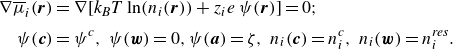 \begin{align} \nabla \overline{\mu }_{i}\!\left(\boldsymbol{r}\right) & = \nabla \!\left[k_{\textit{B}}T\ln \!\left(n_{i}\!\left(\boldsymbol{r}\right)\right)+z_{i}e\,\psi \!\left(\boldsymbol{r}\right)\right]=0; \nonumber \\[4pt] \psi\!\left(\boldsymbol{c}\right) & =\psi ^{c},\ \psi\!\left(\boldsymbol{w}\right)=0,\psi\!\left(\boldsymbol{a}\right)=\zeta,\ n_{i}\!\left(\boldsymbol{c}\right)=n_{i}^{c},\ n_{i}\!\left(\boldsymbol{w}\right)=n_{i}^{\textit{res}}. \end{align}
Here, $k_{\textit{B}}$
is the Boltzmann constant,
$k_{\textit{B}}$
is the Boltzmann constant, $T$
is the absolute temperature,
$T$
is the absolute temperature, $e\enspace$
is the elementary charge,
$e\enspace$
is the elementary charge, $\zeta$
is the electric potential at the slipping plane and
$\zeta$
is the electric potential at the slipping plane and $n_{i}(\boldsymbol{r})$
and
$n_{i}(\boldsymbol{r})$
and $z_{i}$
are respectively the ion density function and valence number of the ith species. First, we will derive an explicit relationship between the ion density function and the electric potential field. We begin by integrating (A1) in the radial coordinate
$z_{i}$
are respectively the ion density function and valence number of the ith species. First, we will derive an explicit relationship between the ion density function and the electric potential field. We begin by integrating (A1) in the radial coordinate
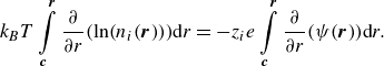 \begin{equation} k_{\textit{B}}T\int\limits_{\boldsymbol{c}}^{\boldsymbol{r}}\frac{\partial }{\partial r}\!\left(\ln \!\left(n_{i}\!\left(\boldsymbol{r}\right)\right)\right)\!\mathrm{d}r=-z_{i}e\int\limits_{\boldsymbol{c}}^{\boldsymbol{r}}\frac{\partial }{\partial r}\!\left(\psi\!\left(\boldsymbol{r}\right)\right)\!\mathrm{d}r .\end{equation}
Evaluating (A2), we may express the ion density function in terms of the ion density at the axial centreline, the electric potential at the axial centreline and the electric potential field
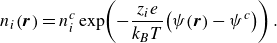 \begin{equation} n_{i}\!\left(\boldsymbol{r}\right)=n_{i}^{c}\exp\!\left(-\frac{z_{i}e}{k_{\textit{B}}T}\!\left(\psi\!\left(\boldsymbol{r}\right)-\psi ^{c}\right)\right) .\end{equation}
We derive a relation between the ion density at the axial centreline and the ion density in the reservoir. To this end, we rearrange (A1) as
 \begin{equation} k_{\textit{B}}T\nabla \!\left(\ln \!\left(n_{i}\!\left(\boldsymbol{r}\right)\right)\right)=-z_{i}e\nabla \!\left(\psi\!\left(\boldsymbol{r}\right)\right) .\end{equation}
Next, define $\boldsymbol{x}\colon \{[0,1]\rightarrow [\boldsymbol{c},\boldsymbol{w}]| \nabla _{\boldsymbol{x}}\,\overline{\mu }_{i}(\boldsymbol{r})=0\}$
as a path between the axial centreline and the reservoir at a constant electrochemical potential. Integrating (A4) along
$\boldsymbol{x}\colon \{[0,1]\rightarrow [\boldsymbol{c},\boldsymbol{w}]| \nabla _{\boldsymbol{x}}\,\overline{\mu }_{i}(\boldsymbol{r})=0\}$
as a path between the axial centreline and the reservoir at a constant electrochemical potential. Integrating (A4) along $\boldsymbol{x}$
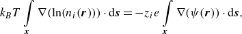 \begin{equation} k_{\textit{B}}T\int\limits_{\boldsymbol{x}}\nabla \!\left(\ln \!\left(n_{i}\!\left(\boldsymbol{r}\right)\right)\right)\cdot \mathrm{d}\boldsymbol{s}=-z_{i}e \int\limits_{\boldsymbol{x}}\nabla \!\left(\psi\!\left(\boldsymbol{r}\right)\right)\cdot \mathrm{d}\boldsymbol{s}, \end{equation}
we arrive at the following formulation relating the ion density at the axial centreline, the ion density in the reservoir and the axial centreline potential:
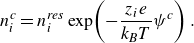 \begin{equation} n_{i}^{c}=n_{i}^{\textit{res}}\exp\!\left(-\frac{z_{i}e}{k_{\textit{B}}T}\psi ^{c}\right) .\end{equation}
From (A3) and (A6), the electric charge density can be expressed as
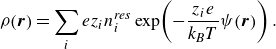 \begin{equation} \rho\!\left(\boldsymbol{r}\right)=\sum _{i}ez_{i}n_{i}^{\textit{res}}\exp\!\left(-\frac{z_{i}e}{k_{\textit{B}}T}\psi\!\left(\boldsymbol{r}\right)\right) .\end{equation}
Given this formulation of the electric charge density, we shall now derive an expression for the electric potential field $\psi (\boldsymbol{r})$
using the Debye–Hückel approximation. First, we apply the Debye–Hückel approximation to (A7)
$\psi (\boldsymbol{r})$
using the Debye–Hückel approximation. First, we apply the Debye–Hückel approximation to (A7)
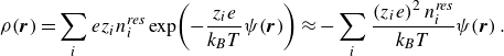 \begin{equation} \rho\!\left(\boldsymbol{r}\right)=\sum _{i}e z_{i}n_{i}^{\textit{res}}\exp\!\left(-\frac{z_{i}e}{k_{\textit{B}}T}\psi\! \left(\boldsymbol{r}\right)\right)\approx -\sum _{i}\frac{\left(z_{i}e\right)^{2}n_{i}^{\textit{res}}}{k_{\textit{B}}T}\psi \!\left(\boldsymbol{r}\right) .\end{equation}
Let $\varepsilon _{e}$
denote the permittivity of the fluid, which is assumed to be uniform throughout the channel. We may then define the Debye length as
$\varepsilon _{e}$
denote the permittivity of the fluid, which is assumed to be uniform throughout the channel. We may then define the Debye length as
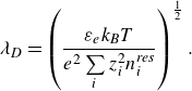 \begin{equation} \lambda _{D}=\left(\frac{\varepsilon _{e}k_{\textit{B}}T}{e^{2}\sum\limits _{i}z_{i}^{2}n_{i}^{\textit{res}}}\right)^{\frac{1}{2}} .\end{equation}
Note that (A9) is a Debye length defined in terms of the ion density in an electroneutral reservoir. Proceeding with the derivation, we henceforth consider a long, thin channel, so we neglect near-channel end edge effects (e.g. transition to the reservoir). Namely, we consider locations in the channel of sufficient distance from the ends of the channel so that we may approximate $\psi (\boldsymbol{r})\approx \psi (r)$
. Substituting (A8) and (A9) into Gauss’s law
$\psi (\boldsymbol{r})\approx \psi (r)$
. Substituting (A8) and (A9) into Gauss’s law
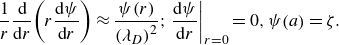 \begin{equation} \frac{1}{r}\frac{{\rm d}}{{\rm d}r}\!\left(r\frac{{\rm d}\psi }{{\rm d}r}\right)\approx \frac{\psi\! \left(r\right)}{\left(\lambda _{D}\right)^{2}};\left.\frac{{\rm d}\psi }{{\rm d}r}\right| _{r=0}=0,\psi\!\left(a\right)=\zeta .\end{equation}
Solving (A10) with the Frobenius method
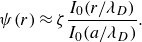 \begin{equation} \psi\!\left(r\right)\approx \zeta \frac{I_{0}\!\left(r/\lambda _{D}\right)}{I_{0}\!\left(a/\lambda _{D}\right)} .\end{equation}
Equation (A11) analytically describes the electric potential field under the Debye–Hückel approximation. Further, evaluating (A11) at $r=0$
, we see that the centreline electric potential is given by
$r=0$
, we see that the centreline electric potential is given by
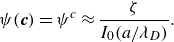 \begin{equation} \psi\!\left(\boldsymbol{c}\right)=\psi ^{c}\approx \frac{\zeta }{I_{0}\!\left(a/\lambda _{D}\right)} .\end{equation}
That is, $\psi ^{c}$
reaches a maximum value of
$\psi ^{c}$
reaches a maximum value of $\zeta$
for a very thick EDL relative to the tube radius then decays rapidly (nearly exponentially) as
$\zeta$
for a very thick EDL relative to the tube radius then decays rapidly (nearly exponentially) as $a/\lambda _{D}$
grows large. Next, using the expression for the electric potential field in (A11), we shall now derive a description of the EOF velocity profile. Assuming the external electric field
$a/\lambda _{D}$
grows large. Next, using the expression for the electric potential field in (A11), we shall now derive a description of the EOF velocity profile. Assuming the external electric field $E$
is uniform and acts solely in the axial direction, the Stokes flow equation can be expressed as
$E$
is uniform and acts solely in the axial direction, the Stokes flow equation can be expressed as
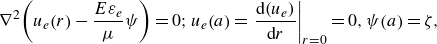 \begin{equation} \nabla ^{2}\!\left(u_{e}\!\left(r\right)-\frac{E\varepsilon _{e}}{\mu }\psi \right)=0;u_{e}\!\left(a\right)=\left.\frac{{\rm d}\!\left(u_{e}\right)}{{\rm d}r}\right| _{r=0}=0,\psi\!\left(a\right)=\zeta, \end{equation}
with $\mu$
denoting the dynamic viscosity of the fluid. The solution to (A13) is
$\mu$
denoting the dynamic viscosity of the fluid. The solution to (A13) is
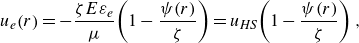 \begin{equation} u_{e}\!\left(r\right)=-\frac{\zeta E\varepsilon _{e}}{\mu }\!\left(1-\frac{\psi\!\left(r\right)}{\zeta }\right)=u_{\textit{HS}}\!\left(1-\frac{\psi\!\left(r\right)}{\zeta }\right), \end{equation}
where $u_{\textit{HS}}=-\mu ^{-1}\zeta E\varepsilon _{e}$
is the Helmholtz–Smoluchowski velocity scale. Substituting (A11) into (A14)
$u_{\textit{HS}}=-\mu ^{-1}\zeta E\varepsilon _{e}$
is the Helmholtz–Smoluchowski velocity scale. Substituting (A11) into (A14)
 \begin{equation} u_{e}\!\left(r\right)=-\frac{\zeta E\varepsilon _{e}}{\mu }\!\left(1-\frac{I_{0}\!\left(r/\lambda _{D}\right)}{I_{0}\!\left(a/\lambda _{D}\right)}\right)=u_{\textit{HS}}\!\left(1-\frac{I_{0}\!\left(r/\lambda _{D}\right)}{I_{0}\!\left(a/\lambda _{D}\right)}\right) .\end{equation}
Equation (A15) provides an analytical formulation for the EOF velocity profile for an EDL of arbitrary thickness relative to the channel radius. We achieve this by expressing (A15) in terms of a Debye length defined using the ion density in an electroneutral reservoir at equilibrium with the channel (cf. (A9)).
Note (A15) is nearly identical to the EOF velocity profile reported by Rice & Whitehead (Reference Rice and Whitehead1965). However, Rice & Whitehead considered a theoretical cylindrical tube without an associated electroneutral reservoir for their derivation. As such, Rice & Whitehead used a Debye length defined simply through a ‘bulk ion density’. We interpret the latter as a theoretical point where the ion density is electroneutral. We note that, when an EDL is highly overlapped with itself, there is net charge throughout the regions of the channel occupied by diffuse ions. Our approach here avoids these technicalities by considering a channel in equilibrium with an electroneutral reservoir. In the end, we note that equation (A15) is equivalent to Rice & Whitehead’s (Reference Rice and Whitehead1965) formulation for the EOF velocity profile apart from this small discrepancy in the definition of the Debye length.


 Open access