





1. Introduction
Self-aligning particles are defined as rigid bodies that reach an equilibrium orientation in a simple shear flow (SSF) in the absence of any external forces or torques (Bretherton Reference Bretherton1962; Singh, Koch & Stroock Reference Singh, Koch and Stroock2013; Borker, Stroock & Koch Reference Borker, Stroock and Koch2018). Unlike most rigid particles, which undergo continuous rotation in shear flows, self-aligning particles (SAPs) permanently align near the fluid lamellae. This behaviour arises purely from particle geometry and hydrodynamic interactions (HIs) with the background flow. Particularly, ring-shaped SAPs, such as the example shown in figure 1(a), exhibit this self-alignment phenomenon at moderate aspect ratios for a diverse range of cross-sectional shapes (Borker et al. Reference Borker, Stroock and Koch2018, Reference Borker, Stroock and Koch2024). Furthermore, these ring-shaped SAPs exhibit remarkable stability, maintaining their aligned orientation even amidst secondary disturbances induced by perturbations to the shear flow, interparticle interactions or Brownian motion (Borker, Stroock & Koch Reference Borker, Stroock and Koch2024). While the existence and robustness of self-alignment have been established, its quantitative implications on the suspension rheology remain unexplored. In particular, it is not known whether suppressing tumbling fundamentally alters the mechanisms by which particles generate stresses in a suspension, or how permanent alignment changes the emergence or strength of non-Newtonian behaviour. Addressing these questions is the central goal of the present work.
In this study, we use dynamic numerical simulations to demonstrate that permanent alignment leads to a qualitatively distinct rheological response: SAP suspensions generate significantly smaller shear stresses than suspensions of equivalent tumbling particles, while simultaneously producing larger normal stress differences. This arises from the fundamentally distinct stress-generating mechanisms in SAP suspensions compared with those operative in tumbling-particle suspensions. In particular, for SAPs at moderate aspect ratios, the dipole per unit length along the centreline of the ring’s cross-section is the primary contributor to particle stresses, whereas in tumbling rings of comparable aspect ratio the contribution from the force per unit length dominates. This difference leads to shear stresses that are smaller by approximately an order of magnitude for SAPs. The asymmetric equilibrium orientation of SAPs about the gradient–vorticity plane also generates normal stresses from purely hydrodynamic effects unlike the normal stresses generated in tumbling-particle suspensions, which require irreversible effects like collisions or Brownian motion (Petrie Reference Petrie1999; Borker & Koch Reference Borker and Koch2023). As a consequence of this difference, normal stresses in SAP suspensions scale linearly with particle number density, in contrast to the quadratic scaling observed in suspensions of non-Brownian tumbling particles, causing SAP suspensions to exhibit non-Newtonian behaviour at moderate particle concentrations.
We investigate the unusual rheology of a suspension of SAPs using the slender body theory (SBT) framework (Batchelor Reference Batchelor1970; Borker & Koch Reference Borker and Koch2019), a methodology previously employed to compute the rheology of suspensions containing tumbling fibres (Rahnama, Koch & Shaqfeh Reference Rahnama, Koch and Shaqfeh1995; Mackaplow & Shaqfeh Reference Mackaplow and Shaqfeh1996; Butler & Shaqfeh Reference Butler and Shaqfeh2002; Snook et al. Reference Snook, Davidson, Butler, Pouliquen and Guazzelli2014) or rings (Borker & Koch Reference Borker and Koch2023). Within this framework, we study pairwise interactions (PIs) between SAPs, as well as PIs between a SAP and a tumbling torus, to compute particle stresses at dilute concentrations. These simulations are also used to establish design rules for passively tuning both the rheology and orientational microstructure of suspensions by selecting specific particle geometries or by incorporating controlled fractions of tumbling particles into SAP suspensions. We further investigate multiparticle interactions (MIs) between SAPs in a periodic domain to characterize suspension rheology at moderate particle number densities. Boundary element method (BEM) simulations are also employed to compute particle stresses on a wide range of ring-shaped geometries, enabling us to generalize our results to other families of SAPs. Brownian dynamics (BD) simulations are also conducted to quantify the shear rate dependence of the shear viscosity and normal stresses in the suspension associated with Brownian forces acting on particles that are sufficiently small. Our findings here indicate that a suspension of SAPs not only exhibits an anisotropic orientational microstructure, but also has a distinct non-Newtonian behaviour compared with suspensions of tumbling particles.
Fabrication methods for SAPs include multistep photolithography (Branch Reference Branch2016) or 3D printing (Di Giusto, Bergougnoux & Guazzelli Reference Di Giusto, Bergougnoux and Guazzelli2025). Their permanent alignment could enable the production of composites with highly anisotropic microstructures using a suspension of SAPs (Borker et al. Reference Borker, Stroock and Koch2024). Such anisotropies would be difficult to achieve with traditional high-aspect-ratio particles, such as fibres or discs, as they only temporarily align near fluid lamellae (Yasuda, Mori & Nakamura Reference Yasuda, Mori and Nakamura2002; Borker et al. Reference Borker, Stroock and Koch2024). Such materials with precise control of the orientational microstructure can be manufactured through conventional processing flow techniques like injection moulding, casting or thin film coating (Dealy & Wissbrun Reference Dealy and Wissbrun2012) which have been successful in manufacturing composites infused with tumbling fibres (Lundell, Söderberg & Alfredsson Reference Lundell, Söderberg and Alfredsson2011) or flakes (Mansouri et al. Reference Mansouri, Burford, Cheng and Hanu2005; Yu et al. Reference Yu, Ramesh, Itkis, Bekyarova and Haddon2007). The SAPs that are also conductive can be used to make lightweight heat spreader materials crucial for thermal management in electric vehicle batteries (Feng et al. Reference Feng, Wei, Sun, Wang, Lan, Shang, Ding, Bai, Yang and Yang2022; He et al. Reference He, Zhang, Wang, Zhang, Xiao, Niu and Yao2022) and 5G devices (Niu et al. Reference Niu, Ren, Guo, Małycha, Orzechowski and Bai2020). Alternatively, SAPs with specific surface functionalities could find utility in fabricating highly porous materials tailored for catalytic applications, leveraging the precise alignment and high surface area to volume ratio of high aspect ratio ring-shaped SAPs (Wittstock et al. Reference Wittstock, Zielasek, Biener, Friend and Bäumer2010; Pan et al. Reference Pan, Paschoalino, Bayram, Blum and Mauzeroll2019).
The long direction(s) of thin particles (rod-like or disc-like) spends a long time normal to the gradient direction $\hat {\boldsymbol{e}}_2$
, but eventually rotates across the flow–vorticity plane, referred henceforth as a tumble/flip (Jeffery Reference Jeffery1922; Bretherton Reference Bretherton1962). In contrast, SAPs permanently align near the flow–vorticity (
$\hat {\boldsymbol{e}}_2$
, but eventually rotates across the flow–vorticity plane, referred henceforth as a tumble/flip (Jeffery Reference Jeffery1922; Bretherton Reference Bretherton1962). In contrast, SAPs permanently align near the flow–vorticity ( $\hat {\boldsymbol{e}}_1\hat {\boldsymbol{e}}_3$
) plane deviating from the norm of continuous rotation exhibited by most other rigid bodies. The longitudinal direction of axisymmetric SAPs aligns in the extensional quadrant of the SSF, as depicted in figure 1(b), and subtends a small angle
$\hat {\boldsymbol{e}}_1\hat {\boldsymbol{e}}_3$
) plane deviating from the norm of continuous rotation exhibited by most other rigid bodies. The longitudinal direction of axisymmetric SAPs aligns in the extensional quadrant of the SSF, as depicted in figure 1(b), and subtends a small angle $\delta$
with the flow direction. The right-hand coordinate system formed by the flow (
$\delta$
with the flow direction. The right-hand coordinate system formed by the flow ( $\hat {\boldsymbol{e}}_1$
), gradient (
$\hat {\boldsymbol{e}}_1$
), gradient ( $\hat {\boldsymbol{e}}_2$
) and vorticity (–
$\hat {\boldsymbol{e}}_2$
) and vorticity (– $\hat {\boldsymbol{e}}_3$
) directions of the SSF is used as the fixed reference frame throughout this study. The orientation of a ring’s symmetry axis is termed as
$\hat {\boldsymbol{e}}_3$
) directions of the SSF is used as the fixed reference frame throughout this study. The orientation of a ring’s symmetry axis is termed as $\boldsymbol{p}$
and at its equilibrium orientation is denoted by
$\boldsymbol{p}$
and at its equilibrium orientation is denoted by $\boldsymbol{p}_S=[-\sin (\delta ), \cos (\delta ), 0]$
, as depicted in figure 1(b).
$\boldsymbol{p}_S=[-\sin (\delta ), \cos (\delta ), 0]$
, as depicted in figure 1(b).
For an axisymmetric particle, the unit vector along its axis of symmetry, $\boldsymbol{p}$
, describes the particle orientation and its dynamics are governed by Jeffery’s equation,
$\boldsymbol{p}$
, describes the particle orientation and its dynamics are governed by Jeffery’s equation,
 \begin{eqnarray} \frac {{\rm d}\boldsymbol{p}}{{\rm d}t} = \boldsymbol{p}\boldsymbol{\cdot }\boldsymbol{\varOmega }_\infty + \lambda \left (\boldsymbol{p\boldsymbol{\cdot }E}_\infty - \boldsymbol{ppp\boldsymbol{\cdot }E}_\infty \right ), \end{eqnarray}
where $\boldsymbol{\varOmega }_\infty$
is the vorticity tensor,
$\boldsymbol{\varOmega }_\infty$
is the vorticity tensor, $\boldsymbol{E}_\infty$
is the rate of strain tensor and
$\boldsymbol{E}_\infty$
is the rate of strain tensor and $\lambda$
is the Bretherton parameter that depends solely on the particle geometry (Jeffery Reference Jeffery1922; Bretherton Reference Bretherton1962). For most axisymmetric particles,
$\lambda$
is the Bretherton parameter that depends solely on the particle geometry (Jeffery Reference Jeffery1922; Bretherton Reference Bretherton1962). For most axisymmetric particles, $|\lambda |\lt 1$
, and the solution of (1.1) corresponds to periodic Jeffery orbits (Jeffery Reference Jeffery1922). The time evolution of the azimuthal angle,
$|\lambda |\lt 1$
, and the solution of (1.1) corresponds to periodic Jeffery orbits (Jeffery Reference Jeffery1922). The time evolution of the azimuthal angle, $\phi$
, and polar angle,
$\phi$
, and polar angle, $\theta$
describing the particle orientation is then given by
$\theta$
describing the particle orientation is then given by
 \begin{eqnarray} \tan \left (\phi \right )&=& \delta _T \tan \left ( \frac {t}{\left (\delta _T + \delta _T^{-1}\right )} + \bar {\tau }\right )\! , \nonumber \\\tan \left (\theta \right ) &=& \frac {\bar {C} \delta _T}{\sqrt {\delta _T^2\cos ^2\left (\phi \right ) + \sin ^2\left (\phi \right )}} , \end{eqnarray}
where $t$
is the non-dimensional time,
$t$
is the non-dimensional time, $\bar {C}$
is the orbit constant,
$\bar {C}$
is the orbit constant, $\bar {\tau }$
is the phase angle and
$\bar {\tau }$
is the phase angle and $\delta _T=\sqrt {(1+\lambda )/(1-\lambda )}$
is the inverse effective aspect ratio of the particle. The magnitude of
$\delta _T=\sqrt {(1+\lambda )/(1-\lambda )}$
is the inverse effective aspect ratio of the particle. The magnitude of $\delta _T$
characterizes the fraction of time a particle spends tumbling or flipping during one Jeffery period. For tumbling particles, this fraction of time spent in flipping plays a central role in determining the particle-induced stresses in the suspension (Rahnama et al. Reference Rahnama, Koch and Shaqfeh1995; Borker & Koch Reference Borker and Koch2023), and will be important in later discussions.
$\delta _T$
characterizes the fraction of time a particle spends tumbling or flipping during one Jeffery period. For tumbling particles, this fraction of time spent in flipping plays a central role in determining the particle-induced stresses in the suspension (Rahnama et al. Reference Rahnama, Koch and Shaqfeh1995; Borker & Koch Reference Borker and Koch2023), and will be important in later discussions.
When $|\lambda |\gt 1$
, the solution to (1.1) no longer corresponds to periodic orbits and instead converges to one of the fixed nodes
$|\lambda |\gt 1$
, the solution to (1.1) no longer corresponds to periodic orbits and instead converges to one of the fixed nodes $\pm \boldsymbol{p}_S$
. The transient solution in this regime is given by
$\pm \boldsymbol{p}_S$
. The transient solution in this regime is given by
 \begin{eqnarray} \tan \left (\phi \right )&=& - \tan (\delta ) \left (\frac {\beta + \exp \left (\textit{sign}(\lambda )\sqrt {\lambda ^2-1}t\right )}{\beta - \exp \left (\textit{sign}(\lambda )\sqrt {\lambda ^2-1}t\right )} \right ) \!, \nonumber \\\tan \left (\theta \right ) &=& \frac {\bar {C}}{\sqrt {|\tan ^2(\delta )\cos ^2\left (\phi \right ) - \sin ^2\left (\phi \right ))|}} , \end{eqnarray}
where
 \begin{align} \begin{split} \beta = (\tan (\phi _0) - \tan (\delta ))/(\tan (\phi _0) + \tan (\delta )),\\\bar {C} = \tan (\theta _0) \sqrt {|\tan ^2(\delta )\cos ^2(\phi_0 ) - \sin ^2(\phi_0 ))|} \end{split} \end{align}
is the trajectory constant, $\phi _0$
is the initial azimuthal angle and
$\phi _0$
is the initial azimuthal angle and $\theta _0$
is the initial polar angle of the particle orientation. Ring-shaped SAPs satisfy
$\theta _0$
is the initial polar angle of the particle orientation. Ring-shaped SAPs satisfy $\lambda \leqslant -1$
, whereas fibre-like SAPs described in Bretherton (Reference Bretherton1962) have
$\lambda \leqslant -1$
, whereas fibre-like SAPs described in Bretherton (Reference Bretherton1962) have $\lambda \geq 1$
. For ring-shaped SAPs considered in this work, (1.3) indicates that at long times the azimuthal angle
$\lambda \geq 1$
. For ring-shaped SAPs considered in this work, (1.3) indicates that at long times the azimuthal angle $\phi$
approaches
$\phi$
approaches $-\delta$
(or
$-\delta$
(or $(\pi -\delta )$
depending on the initial orientation), while the polar angle
$(\pi -\delta )$
depending on the initial orientation), while the polar angle $\theta$
approaches
$\theta$
approaches $\pi /2$
. This corresponds to the equilibrium orientation
$\pi /2$
. This corresponds to the equilibrium orientation $\boldsymbol{p}_S$
. The equilibrium alignment angle
$\boldsymbol{p}_S$
. The equilibrium alignment angle $\delta$
is related to the Bretherton parameter
$\delta$
is related to the Bretherton parameter $\lambda$
through
$\lambda$
through $\delta =(1/2)\cos ^{-1}(-1/\lambda )$
(Singh et al. Reference Singh, Koch and Stroock2013; Borker et al. Reference Borker, Stroock and Koch2018).
$\delta =(1/2)\cos ^{-1}(-1/\lambda )$
(Singh et al. Reference Singh, Koch and Stroock2013; Borker et al. Reference Borker, Stroock and Koch2018).
(a) Schematic depicting the coordinate system; a T-ring that can self-align at aspect ratios greater than or equal to $A^*=26$
, rotating slower than an equivalent tumbler (ET) for
$A^*=26$
, rotating slower than an equivalent tumbler (ET) for $A\lt A^*$
. The orientation vector
$A\lt A^*$
. The orientation vector $\boldsymbol{p}$
and the vector denoting the centreline
$\boldsymbol{p}$
and the vector denoting the centreline $\boldsymbol{r}_{\!c}$
is also shown. (b) Schematic of a SAP in its equilibrium orientation,
$\boldsymbol{r}_{\!c}$
is also shown. (b) Schematic of a SAP in its equilibrium orientation, $\boldsymbol{p}_S$
, where the plane of the ring makes an angle
$\boldsymbol{p}_S$
, where the plane of the ring makes an angle $\delta$
with the flow–vorticity plane. Equivalently the orientation vector
$\delta$
with the flow–vorticity plane. Equivalently the orientation vector $\boldsymbol{p}$
makes an angle
$\boldsymbol{p}$
makes an angle $\delta$
with the gradient direction. The unstable orientation of an SAP, denoted by
$\delta$
with the gradient direction. The unstable orientation of an SAP, denoted by $\boldsymbol{p}_U$
, is also shown.
$\boldsymbol{p}_U$
, is also shown.

We investigate rings whose cross-sections resemble an inverted alphabet ‘T’, shown in figure 1(a), and refer to these geometries as T-rings. The T-rings serve as model geometries to elucidate the qualitative nature of particle stresses in a suspension of SAPs. A T-ring rotates like an equivalent torus when the aspect ratio $A$
is much smaller than a critical aspect ratio,
$A$
is much smaller than a critical aspect ratio, $A^*$
; rotates significantly slower than a torus when
$A^*$
; rotates significantly slower than a torus when $(A^*-A)\ll A^*$
; and self-aligns when
$(A^*-A)\ll A^*$
; and self-aligns when $A$
is greater than or equal to
$A$
is greater than or equal to $A^*$
, making an angle
$A^*$
, making an angle $\delta$
with the flow–vorticity plane, as shown in figure 1(b). Here,
$\delta$
with the flow–vorticity plane, as shown in figure 1(b). Here, $A$
is the particle aspect ratio defined as the ratio of the particle’s extent normal and parallel to the axis of symmetry of the ring. The critical aspect ratio
$A$
is the particle aspect ratio defined as the ratio of the particle’s extent normal and parallel to the axis of symmetry of the ring. The critical aspect ratio $A^*$
is the aspect ratio at which the particle is perfectly aligned in the flow–vorticity plane. The equilibrium angle reaches a peak value at
$A^*$
is the aspect ratio at which the particle is perfectly aligned in the flow–vorticity plane. The equilibrium angle reaches a peak value at $A=55$
and gradually decreases with further increase in the aspect ratio, as depicted in figure 2. This qualitative dependence of the alignment angle on the particle aspect ratio holds true for other ring-shaped SAPs as shown in figure 3 of Borker et al. (Reference Borker, Stroock and Koch2024). For ring-shaped particles, the Bretherton parameter (Bretherton Reference Bretherton1962; Singh et al. Reference Singh, Koch and Stroock2013; Borker et al. Reference Borker, Stroock and Koch2018) takes the form
$A=55$
and gradually decreases with further increase in the aspect ratio, as depicted in figure 2. This qualitative dependence of the alignment angle on the particle aspect ratio holds true for other ring-shaped SAPs as shown in figure 3 of Borker et al. (Reference Borker, Stroock and Koch2024). For ring-shaped particles, the Bretherton parameter (Bretherton Reference Bretherton1962; Singh et al. Reference Singh, Koch and Stroock2013; Borker et al. Reference Borker, Stroock and Koch2018) takes the form
 \begin{eqnarray} \lambda = -1 + \frac {C_\lambda }{A^2}\left (\ln (8A)-\frac {3}{2}\right ) - \frac {C_\alpha }{A}, \end{eqnarray}
where $C_\lambda$
and
$C_\lambda$
and $C_\alpha$
are constants that only depend on the particle geometry (Borker et al. Reference Borker, Stroock and Koch2024) and can be evaluated using the BEM (Borker et al. Reference Borker, Stroock and Koch2018). For a torus, the values
$C_\alpha$
are constants that only depend on the particle geometry (Borker et al. Reference Borker, Stroock and Koch2024) and can be evaluated using the BEM (Borker et al. Reference Borker, Stroock and Koch2018). For a torus, the values $C_\lambda =(3/2)$
and
$C_\lambda =(3/2)$
and $C_\alpha =0$
were derived from SBT (Borker & Koch Reference Borker and Koch2019), implying that
$C_\alpha =0$
were derived from SBT (Borker & Koch Reference Borker and Koch2019), implying that $\lambda \gt -1$
for all aspect ratios and that a torus cannot self-align. The value of
$\lambda \gt -1$
for all aspect ratios and that a torus cannot self-align. The value of $\lambda$
for rings with various other cross-sectional shapes is available in Borker et al. (Reference Borker, Stroock and Koch2018, Reference Borker, Stroock and Koch2024). The critical aspect ratio
$\lambda$
for rings with various other cross-sectional shapes is available in Borker et al. (Reference Borker, Stroock and Koch2018, Reference Borker, Stroock and Koch2024). The critical aspect ratio $A^*$
for ring-shaped SAPs is the aspect ratio for which
$A^*$
for ring-shaped SAPs is the aspect ratio for which $\lambda =-1$
and is given by the solution of the implicit equation
$\lambda =-1$
and is given by the solution of the implicit equation $C_\alpha A^* = C_\lambda (\ln (8A^*)-3/2)$
. The simulations of Borker et al. (Reference Borker, Stroock and Koch2018, Reference Borker, Stroock and Koch2024) indicate that
$C_\alpha A^* = C_\lambda (\ln (8A^*)-3/2)$
. The simulations of Borker et al. (Reference Borker, Stroock and Koch2018, Reference Borker, Stroock and Koch2024) indicate that $C_\lambda$
is typically
$C_\lambda$
is typically $O(1)$
and the value of
$O(1)$
and the value of $A^*$
is typically large. This indicates that
$A^*$
is typically large. This indicates that $C_\alpha =O(1/A^*)\ll 1$
(ignoring the logarithmic term) is numerically small for most SAPs. The fact that
$C_\alpha =O(1/A^*)\ll 1$
(ignoring the logarithmic term) is numerically small for most SAPs. The fact that $C_\alpha =O(1/A^*)\ll 1$
will be an important factor while comparing the magnitude of stresses between SAPs and ETs.
$C_\alpha =O(1/A^*)\ll 1$
will be an important factor while comparing the magnitude of stresses between SAPs and ETs.
Comparision of the time period for Tori (o) and tumbling T-rings ( $\square$
) with
$\square$
) with $A\lt A^*$
and the magnitude of the equilibrium angle
$A\lt A^*$
and the magnitude of the equilibrium angle $\delta$
for SAPs (
$\delta$
for SAPs ( $\square$
), i.e. T-rings with
$\square$
), i.e. T-rings with $A\geqslant A^*$
. The time period of rotation for SAPs is infinite as they remain permanently aligned at their equilibrium orientation.
$A\geqslant A^*$
. The time period of rotation for SAPs is infinite as they remain permanently aligned at their equilibrium orientation.

Equation (1.5) can be used to derive the scaling of the time period for tumbling particles and the alignment angle for SAPs with $A$
, which are depicted in figure 2. Ignoring the logarithmic terms in (1.5) simplifies the scaling arguments of several quantities of interest throughout the remainder of the paper. The time-period,
$A$
, which are depicted in figure 2. Ignoring the logarithmic terms in (1.5) simplifies the scaling arguments of several quantities of interest throughout the remainder of the paper. The time-period, $4\pi /\sqrt {1-\lambda ^2}$
, of a torus is linearly proportional to the aspect ratio
$4\pi /\sqrt {1-\lambda ^2}$
, of a torus is linearly proportional to the aspect ratio $A$
(Borker & Koch 2019, Reference Borker and Koch2023). The time period for tumbling T-rings far away from the critical aspect ratio, i.e.
$A$
(Borker & Koch 2019, Reference Borker and Koch2023). The time period for tumbling T-rings far away from the critical aspect ratio, i.e. $(A^*-A)=O(A^*)$
, is also proportional to
$(A^*-A)=O(A^*)$
, is also proportional to $A$
. The scaling for tumbling T-rings and SAPs near the critical aspect ratio
$A$
. The scaling for tumbling T-rings and SAPs near the critical aspect ratio $A=A^*$
can be obtained by simplifying the expression for the Bretherton parameter through the substitution of
$A=A^*$
can be obtained by simplifying the expression for the Bretherton parameter through the substitution of $C_\alpha$
in terms of
$C_\alpha$
in terms of $A^*$
and
$A^*$
and $C_\lambda$
in (1.5):
$C_\lambda$
in (1.5):
 \begin{eqnarray} \lambda = -1 + \frac {C_\lambda }{A^2}\left (\left (\ln (8A)-\frac {3}{2}\right ) - \frac {A}{A^*}\left (\ln (8A^*)-\frac {3}{2}\right )\right )\!. \end{eqnarray}
Due to the slow change in the logarithmic term, we can use the Taylor expansion $\ln (8A)\approx \ln (8A^*) + \Delta A/A^*$
to further simplify the expression,
$\ln (8A)\approx \ln (8A^*) + \Delta A/A^*$
to further simplify the expression,
 \begin{eqnarray} \lambda \approx -1 - C_\lambda \left (\ln (8A^*)-\frac {5}{2}\right ) \left (\frac {\Delta A}{A^*}\frac {1}{A^2}\right ), \end{eqnarray}
where $\Delta A=A-A^*$
. Equation (1.7) has the correct scaling with the aspect ratio as
$\Delta A=A-A^*$
. Equation (1.7) has the correct scaling with the aspect ratio as $A\rightarrow A^*$
and also as
$A\rightarrow A^*$
and also as $A\rightarrow \infty$
. However, (1.7) also captures the predictions for T-rings across the whole range of aspect ratios for T-rings as depicted by the solid lines in figure 2. Unlike the tumbling period of tori that is linear with
$A\rightarrow \infty$
. However, (1.7) also captures the predictions for T-rings across the whole range of aspect ratios for T-rings as depicted by the solid lines in figure 2. Unlike the tumbling period of tori that is linear with $A$
, the time period for tumbling T-rings near the critical aspect ratio, i.e.
$A$
, the time period for tumbling T-rings near the critical aspect ratio, i.e. $(A^*-A)\ll A^*$
, scales as
$(A^*-A)\ll A^*$
, scales as $A\sqrt {A^*/|\Delta A|}$
, indicating the divergence of the time period as
$A\sqrt {A^*/|\Delta A|}$
, indicating the divergence of the time period as $A\rightarrow A^{*-}$
. The T-rings within this range of aspect ratios remain in their flow-aligned state significantly longer than thin-fibre or thin-disk like particles with comparable aspect ratios. For,
$A\rightarrow A^{*-}$
. The T-rings within this range of aspect ratios remain in their flow-aligned state significantly longer than thin-fibre or thin-disk like particles with comparable aspect ratios. For, $A\geqslant A^*$
, the particle remains permanently aligned with an equilibrium angle,
$A\geqslant A^*$
, the particle remains permanently aligned with an equilibrium angle, $\delta =(1/2) \cos ^{-1}(-1/\lambda )\approx \sqrt {(1+\lambda )/(2\lambda )}$
, which scales as
$\delta =(1/2) \cos ^{-1}(-1/\lambda )\approx \sqrt {(1+\lambda )/(2\lambda )}$
, which scales as $\sqrt {\Delta A/A^*}/A$
, according to (1.7). Thus,
$\sqrt {\Delta A/A^*}/A$
, according to (1.7). Thus, $\delta^2$
increases linearly with
$\delta^2$
increases linearly with $A$
when
$A$
when $\Delta A\ll A^*$
, reaches a peak near
$\Delta A\ll A^*$
, reaches a peak near $A=2A^*$
and then scales as
$A=2A^*$
and then scales as $A^{-1}$
when
$A^{-1}$
when $A^*\ll A$
, which is similar to the result obtained from BEM simulation as depicted in figure 2. The overall scaling results are summarized in table 1. Numerical simulations of Borker et al. (Reference Borker, Stroock and Koch2024) indicate that the alignment angle of SAPs,
$A^*\ll A$
, which is similar to the result obtained from BEM simulation as depicted in figure 2. The overall scaling results are summarized in table 1. Numerical simulations of Borker et al. (Reference Borker, Stroock and Koch2024) indicate that the alignment angle of SAPs, $\delta$
, is small for all SAPs discovered to date, causing these particles to exert smaller shear stresses compared with equivalent tumbling particles.
$\delta$
, is small for all SAPs discovered to date, causing these particles to exert smaller shear stresses compared with equivalent tumbling particles.
Scaling for the time-period of rotation ( $\sim 2\pi /\delta _T$
), for tumbling T-rings or tori, and the alignment angle
$\sim 2\pi /\delta _T$
), for tumbling T-rings or tori, and the alignment angle $\delta$
, for self-aligning T-rings.
$\delta$
, for self-aligning T-rings.

The outline of the remainder of the paper is as follows. Section 2 analyses the contribution to particle stresses from isolated non-interacting particles and describes the qualitative mechanisms generating stresses in SAPs. The shear rate dependence of the rheology of SAPs associated with Brownian motion is described in § 3. Section 4.1 presents the contribution to shear stresses from PIs between SAPs. In § 4.2, we present design rules for precisely tuning the shear viscosity and orientational anisotropy of SAP suspensions by adding tumbling particles. The influence of MIs is explored in § 4.3. Section 4.4, examines normal stress differences, including interparticle interactions and discusses the Weissenberg phenomena expected in SAP suspensions. Conclusions and possible directions for future research are summarized in § 5. Throughout this study, the radius of the ring $R$
, defined as half the extent of the ring in its plane, the shear rate of the SSF
$R$
, defined as half the extent of the ring in its plane, the shear rate of the SSF $\gamma$
and the fluid viscosity
$\gamma$
and the fluid viscosity $\mu_{\kern-1pt f}$
are used to non-dimensionalize all pertinent properties.
$\mu_{\kern-1pt f}$
are used to non-dimensionalize all pertinent properties.
2. Rheology of a suspension of isolated SAPs
In this section, we relate the particle stresses to the orientational microstructure, identify the dominant hydrodynamic mechanisms across different aspect ratios of T-rings, and finally generalize these results to other SAP geometries. The hydrodynamic contribution of a particle to the average suspension stress is computed from the stresslet tensor, $\boldsymbol{S}_{\textit{Hyd}}$
, which represents the symmetric, deviatoric part of the first moment of the stresses exerted by the particle on the fluid. For isolated axisymmetric particles,
$\boldsymbol{S}_{\textit{Hyd}}$
, which represents the symmetric, deviatoric part of the first moment of the stresses exerted by the particle on the fluid. For isolated axisymmetric particles, $\boldsymbol{S}_{\textit{Hyd}}$
has the following dependence on the particle orientation
$\boldsymbol{S}_{\textit{Hyd}}$
has the following dependence on the particle orientation $\boldsymbol{p}$
:
$\boldsymbol{p}$
:
 \begin{eqnarray} \boldsymbol{S}_{\textit{Hyd}}\left (\boldsymbol{p}\right ) = \xi _1 \boldsymbol{E}_\infty & + & \xi _2 \left (\boldsymbol{E}_\infty \boldsymbol{\cdot }\boldsymbol{pp} +\boldsymbol{pp}\boldsymbol{\cdot }\boldsymbol{E}_\infty - \frac {2}{3}\boldsymbol{E}_\infty :\boldsymbol{ppI}\right ) \nonumber \\& + & \xi _3 \left (\boldsymbol{E}_\infty : \boldsymbol{pppp} - \frac {1}{3}\boldsymbol{E}_\infty :\boldsymbol{ppI}\right )\!. \end{eqnarray}
Here $\xi _i$
for
$\xi _i$
for $i\in \{1,2,3\}$
are
$i\in \{1,2,3\}$
are $O(\epsilon )$
constants that solely depend on the particle geometry, with
$O(\epsilon )$
constants that solely depend on the particle geometry, with $\xi _1 + \xi _2 = O(1/A^{2})$
(Kim & Karrila Reference Kim and Karrila2013; Borker & Koch Reference Borker and Koch2023) and
$\xi _1 + \xi _2 = O(1/A^{2})$
(Kim & Karrila Reference Kim and Karrila2013; Borker & Koch Reference Borker and Koch2023) and $\epsilon =1/\ln (8A)$
is a small parameter that emerges in the SBT treatment of a ring (Borker & Koch Reference Borker and Koch2019). The constants
$\epsilon =1/\ln (8A)$
is a small parameter that emerges in the SBT treatment of a ring (Borker & Koch Reference Borker and Koch2019). The constants $\xi _1,\xi _2,\xi _3$
, were obtained from SBT of Borker & Koch (Reference Borker and Koch2019) that also includes effects of non-circularity of the cross-sectional shape. The values are given by (A1)–(A3) in Appendix A and they compare well with the corresponding values obtained numerically from BEM calculations as shown in figure 17. As per SBT, the values of
$\xi _1,\xi _2,\xi _3$
, were obtained from SBT of Borker & Koch (Reference Borker and Koch2019) that also includes effects of non-circularity of the cross-sectional shape. The values are given by (A1)–(A3) in Appendix A and they compare well with the corresponding values obtained numerically from BEM calculations as shown in figure 17. As per SBT, the values of $\xi _1$
,
$\xi _1$
, $\xi _2$
and
$\xi _2$
and $\xi _3$
have the same
$\xi _3$
have the same $O(\epsilon )$
scaling with the aspect ratio of the particle for both SAPs and ETs, only differing in their numerical values. This implies that the difference in the magnitude of the particle stresses between these two particles is primarily determined by the difference in their orientational microstructure.
$O(\epsilon )$
scaling with the aspect ratio of the particle for both SAPs and ETs, only differing in their numerical values. This implies that the difference in the magnitude of the particle stresses between these two particles is primarily determined by the difference in their orientational microstructure.
The stresslet for an isolated axisymmetric particle averaged over the steady state orientation distribution is
 \begin{eqnarray} \langle \boldsymbol{S}_{\textit{Hyd}}\rangle _J = \xi _1 \boldsymbol{E}_\infty & + & \xi _2 \left (\boldsymbol{E}_\infty \boldsymbol{\cdot }\langle\, \boldsymbol{pp}\rangle _J+\langle\, \boldsymbol{pp}\rangle _J\boldsymbol{\cdot }\boldsymbol{E}_\infty - \frac {2}{3}\boldsymbol{E}_\infty :\langle\, \boldsymbol{pp}\rangle _J\boldsymbol{I}\right ) \nonumber \\ & + & \xi _3 \left (\boldsymbol{E}_\infty : \langle\, \boldsymbol{pppp} \rangle _J- \frac {1}{3}\boldsymbol{E}_\infty :\langle\, \boldsymbol{pp}\rangle _J\boldsymbol{I}\right ), \end{eqnarray}
where the angular bracket $\langle \boldsymbol{\cdot }\rangle _J$
indicates an average over the steady state orbit distribution and Jeffery rotation for tumblers and corresponds to
$\langle \boldsymbol{\cdot }\rangle _J$
indicates an average over the steady state orbit distribution and Jeffery rotation for tumblers and corresponds to $\boldsymbol{S}_{\textit{Hyd}}$
at
$\boldsymbol{S}_{\textit{Hyd}}$
at $\boldsymbol{p}=\boldsymbol{p}_S$
for SAPs. The particle shear stress
$\boldsymbol{p}=\boldsymbol{p}_S$
for SAPs. The particle shear stress $n\langle S_{\textit{Hyd}}\rangle _J=n\langle \boldsymbol{S}_{\textit{Hyd}}\rangle _J:\hat {\boldsymbol{e}}_1\hat {\boldsymbol{e}}_2$
is directly related to the specific viscosity of the suspension,
$n\langle S_{\textit{Hyd}}\rangle _J=n\langle \boldsymbol{S}_{\textit{Hyd}}\rangle _J:\hat {\boldsymbol{e}}_1\hat {\boldsymbol{e}}_2$
is directly related to the specific viscosity of the suspension,
 \begin{eqnarray} \Delta \mu =\left (\frac {\mu }{\mu_{\kern-1pt f}}-1\right )=n\langle S_{\textit{Hyd}}\rangle _J+O(n^2), \end{eqnarray}
where $n$
is the number density non-dimensionalized by
$n$
is the number density non-dimensionalized by $R^{-3}$
and
$R^{-3}$
and $\mu$
is the shear viscosity of the suspension. The value of
$\mu$
is the shear viscosity of the suspension. The value of $\langle S_{\textit{Hyd}}\rangle _J$
may be expressed explicitly in terms of the azimuthal angle
$\langle S_{\textit{Hyd}}\rangle _J$
may be expressed explicitly in terms of the azimuthal angle $\phi$
and the polar angle
$\phi$
and the polar angle $\theta$
of the particle orientation as
$\theta$
of the particle orientation as
 \begin{eqnarray} \langle S_{\textit{Hyd}}\rangle _J= \left (\frac {\xi _3}{4} \big\langle \sin ^4(\theta )\sin ^2(4\phi )\big\rangle _J- \frac {\xi _2}{2} \big\langle \cos ^2(\theta ) \big\rangle _J\right ) + \frac {1}{2}\left (\xi _1+\xi _2\right ) . \end{eqnarray}
The variation of $\langle S_{\textit{Hyd}}\rangle _J$
with
$\langle S_{\textit{Hyd}}\rangle _J$
with $A$
is depicted in figure 3(a) for SAPs and ETs (Borker & Koch Reference Borker and Koch2023). The steady state orbit distribution for tumbling particles was obtained either through PI simulations of Borker & Koch (Reference Borker and Koch2023) (symbols) or from the Leal–Hinch distribution for weak Brownian motion (Leal & Hinch Reference Leal and Hinch1971) (solid line), both yielding nearly the same magnitude of particle stresses (Borker & Koch Reference Borker and Koch2023).
$A$
is depicted in figure 3(a) for SAPs and ETs (Borker & Koch Reference Borker and Koch2023). The steady state orbit distribution for tumbling particles was obtained either through PI simulations of Borker & Koch (Reference Borker and Koch2023) (symbols) or from the Leal–Hinch distribution for weak Brownian motion (Leal & Hinch Reference Leal and Hinch1971) (solid line), both yielding nearly the same magnitude of particle stresses (Borker & Koch Reference Borker and Koch2023).
Figure 3(a) indicates that SAPs generate much smaller shear stresses in the suspension compared with equivalent tumbling tori of the same aspect ratio. For a tumbling torus, the stresses generated during the short tumbling phase are an order of magnitude greater than the stresses generated during its phase of temporary alignment near the flow–vorticity plane (Rahnama et al. Reference Rahnama, Koch and Shaqfeh1995; Borker & Koch Reference Borker and Koch2023). The greater distortion of streamlines during the tumbling phase causes the higher contribution to the stresses. On the contrary, SAPs remain permanently aligned near the flow–vorticity plane at all times and thereby have a much smaller contribution to $\langle S_{\textit{Hyd}}\rangle _J$
as shown in figure 3(a) for
$\langle S_{\textit{Hyd}}\rangle _J$
as shown in figure 3(a) for $A\gt A^*$
. Therefore, a suspension of SAPs should have a much smaller specific viscosity compared with a suspension of planar tumbling particles of similar aspect ratio at moderate number densities.
$A\gt A^*$
. Therefore, a suspension of SAPs should have a much smaller specific viscosity compared with a suspension of planar tumbling particles of similar aspect ratio at moderate number densities.
Particle shear stresses in SAP suspensions. (a) Particle shear stress $n\langle S_{\textit{Hyd}}\rangle _J$
as a function of the aspect ratio
$n\langle S_{\textit{Hyd}}\rangle _J$
as a function of the aspect ratio $A$
for T-rings (
$A$
for T-rings ( $\square$
) and ETs (o) calculated using orientation distributions obtained from PI simulations (symbols) and Leal and Hinch’s theory for weak Brownian motion (solid line). (b) The contribution from the dipole per unit length,
$\square$
) and ETs (o) calculated using orientation distributions obtained from PI simulations (symbols) and Leal and Hinch’s theory for weak Brownian motion (solid line). (b) The contribution from the dipole per unit length, $\xi _1 + \xi _2$
, (dashed line) and the force per unit length (solid line) for T-rings (thick lines) and a torus (thin lines).
$\xi _1 + \xi _2$
, (dashed line) and the force per unit length (solid line) for T-rings (thick lines) and a torus (thin lines).

The expression in (2.4) reveals that particle-induced shear stresses in SAP suspensions arise from two physically distinct mechanisms. The term $n\xi _3\delta ^2=O(n\epsilon \Delta A/(A^{2}A^*))$
is driven by the force per unit length exerted by the particle on the fluid and is proportional to the difference in the local velocity between the particle and the background SSF at the centreline of the ring. In contrast, the term
$n\xi _3\delta ^2=O(n\epsilon \Delta A/(A^{2}A^*))$
is driven by the force per unit length exerted by the particle on the fluid and is proportional to the difference in the local velocity between the particle and the background SSF at the centreline of the ring. In contrast, the term $n(\xi _1+\xi _2)/2=O(n/A^{2})$
corresponds to the contribution from the dipole per unit length, which arises from the first moment of traction on the particle surface about a moment arm whose length scales with the size of the particle’s cross-section,
$n(\xi _1+\xi _2)/2=O(n/A^{2})$
corresponds to the contribution from the dipole per unit length, which arises from the first moment of traction on the particle surface about a moment arm whose length scales with the size of the particle’s cross-section, $A^{-1}$
. The scaling implies that the dipole per unit length contribution dominates for particles with aspect ratios sufficiently close to
$A^{-1}$
. The scaling implies that the dipole per unit length contribution dominates for particles with aspect ratios sufficiently close to $A^*$
, i.e.
$A^*$
, i.e. $|\Delta A|\ll A^*$
. Boundary element method calculations confirm these scaling arguments and figure 3(b) illustrates the dipole dominated regime for T-ring shaped SAPs in the range
$|\Delta A|\ll A^*$
. Boundary element method calculations confirm these scaling arguments and figure 3(b) illustrates the dipole dominated regime for T-ring shaped SAPs in the range $26\lt A\lt 100$
. To our knowledge, the emergence of a qualitatively distinct stress-generation mechanism associated with the dipole per unit length in rigid particle suspensions has not been reported previously.
$26\lt A\lt 100$
. To our knowledge, the emergence of a qualitatively distinct stress-generation mechanism associated with the dipole per unit length in rigid particle suspensions has not been reported previously.
In the force per unit length dominated regime, $A\gg A^*$
, the shear stresses scale as
$A\gg A^*$
, the shear stresses scale as $n\epsilon /(AA^*)$
and for T-ring shaped SAPs this regime starts around
$n\epsilon /(AA^*)$
and for T-ring shaped SAPs this regime starts around $A=100$
as depicted in figure 3(b). In this regime, the shear stress for these SAPs has the same scaling with
$A=100$
as depicted in figure 3(b). In this regime, the shear stress for these SAPs has the same scaling with $A$
as ETs for which
$A$
as ETs for which $\langle S_{\textit{Hyd}}\rangle _J$
is
$\langle S_{\textit{Hyd}}\rangle _J$
is $O(\epsilon \delta _T)=O(\epsilon /A)$
, derived from an
$O(\epsilon \delta _T)=O(\epsilon /A)$
, derived from an $O(\epsilon )$
stresslet of a tumbling ring multiplied by the
$O(\epsilon )$
stresslet of a tumbling ring multiplied by the $O(1/A)$
tumbling frequency (Rahnama et al. Reference Rahnama, Koch and Shaqfeh1995; Mackaplow & Shaqfeh Reference Mackaplow and Shaqfeh1996; Borker & Koch Reference Borker and Koch2023). However, the numerical value for the particle stresses is smaller for SAPs compared with ETs by a factor of
$O(1/A)$
tumbling frequency (Rahnama et al. Reference Rahnama, Koch and Shaqfeh1995; Mackaplow & Shaqfeh Reference Mackaplow and Shaqfeh1996; Borker & Koch Reference Borker and Koch2023). However, the numerical value for the particle stresses is smaller for SAPs compared with ETs by a factor of $O(1/A^*)\ll 1$
which explains the behaviour shown in figure 3(a). Figure 3(b) further shows that, for
$O(1/A^*)\ll 1$
which explains the behaviour shown in figure 3(a). Figure 3(b) further shows that, for $A\gg 100$
, the force per unit length contributions for SAPs and ETs exhibit identical scaling with the aspect ratio, while the corresponding dipole contributions are negligible in comparison.
$A\gg 100$
, the force per unit length contributions for SAPs and ETs exhibit identical scaling with the aspect ratio, while the corresponding dipole contributions are negligible in comparison.
Tumbling T-rings near the critical aspect ratio, i.e. $|\Delta A|\ll A^*$
and
$|\Delta A|\ll A^*$
and $A\lt A^*$
, also exert much lower stresses than ETs because the particle remains aligned in the flow–vorticity plane for larger portions of the period and the dominant contribution arises from the dipole per unit length, as illustrated in figure 3(b). The scaling of particle shear stresses with the aspect ratio for T-rings and tori is summarized in table 2. Figure 3(a) also depicts the ensemble average stresslet exerted by a sheared suspension of equivalent cylindrical discs (
$A\lt A^*$
, also exert much lower stresses than ETs because the particle remains aligned in the flow–vorticity plane for larger portions of the period and the dominant contribution arises from the dipole per unit length, as illustrated in figure 3(b). The scaling of particle shear stresses with the aspect ratio for T-rings and tori is summarized in table 2. Figure 3(a) also depicts the ensemble average stresslet exerted by a sheared suspension of equivalent cylindrical discs (
 dashed line), where the coefficients $\xi _1$
,
$\xi _1$
, $\xi _2$
and
$\xi _2$
and $\xi _3$
were obtained from BEM calculations (Borker et al. Reference Borker, Stroock and Koch2018) and the orientation distribution corresponds to the Leal–Hinch distribution for weak Brownian motion (Leal & Hinch Reference Leal and Hinch1971). The shear stresses in a suspension of discs, due to their occasional tumbling, are also considerably greater than the corresponding value for SAPs of the same size and aspect ratio.
$\xi _3$
were obtained from BEM calculations (Borker et al. Reference Borker, Stroock and Koch2018) and the orientation distribution corresponds to the Leal–Hinch distribution for weak Brownian motion (Leal & Hinch Reference Leal and Hinch1971). The shear stresses in a suspension of discs, due to their occasional tumbling, are also considerably greater than the corresponding value for SAPs of the same size and aspect ratio.
Scaling for the particle shear stress of isolated particles, $n\langle {S}_{\textit{Hyd}}\rangle _J$
, for T-rings or tori, correct to
$n\langle {S}_{\textit{Hyd}}\rangle _J$
, for T-rings or tori, correct to $O(n)$
.
$O(n)$
.

The dependence of particle shear stress on aspect ratio for other SAP geometries also qualitatively mirrors the trend observed for T-rings. Figure 4 shows $\langle S_{\textit{Hyd}}\rangle _J$
as a function of
$\langle S_{\textit{Hyd}}\rangle _J$
as a function of $A$
for rings of various cross-sectional shapes and their values were obtained using boundary-element method calculations of Borker et al. (Reference Borker, Stroock and Koch2018). For tumbling particles, we used the Leal–Hinch distribution (Leal & Hinch Reference Leal and Hinch1971). The shear stresslet
$A$
for rings of various cross-sectional shapes and their values were obtained using boundary-element method calculations of Borker et al. (Reference Borker, Stroock and Koch2018). For tumbling particles, we used the Leal–Hinch distribution (Leal & Hinch Reference Leal and Hinch1971). The shear stresslet $\langle S_{\textit{Hyd}}\rangle _J$
for all SAPs shown in figure 4 have the same qualitative dependence on the particle aspect ratio as that described for T-rings: the particle stresses are similar to a torus when
$\langle S_{\textit{Hyd}}\rangle _J$
for all SAPs shown in figure 4 have the same qualitative dependence on the particle aspect ratio as that described for T-rings: the particle stresses are similar to a torus when $A\ll A^*$
; are smaller than a torus when
$A\ll A^*$
; are smaller than a torus when $|\Delta A|\ll A^*$
and
$|\Delta A|\ll A^*$
and $A\lt A^*$
; and are much smaller than a torus when the particle self-aligns, i.e.
$A\lt A^*$
; and are much smaller than a torus when the particle self-aligns, i.e. $A\geqslant A^*$
.
$A\geqslant A^*$
.
Particle shear stresses in suspensions of rings of various cross-sectional shapes at different aspect ratios obtained from boundary-element-method simulations described in Borker et al. (Reference Borker, Stroock and Koch2018).

Importantly, figure 4 demonstrates that SAPs with distinct cross-sectional geometries exert shear stresses of comparable magnitude when $\Delta A=O(A^*)$
. In this practically relevant aspect ratio regime, the particle shear stress is dominated by the dipole per unit length along the centreline of the ring. Since this contribution scales with the square of the particle’s cross-sectional size,
$\Delta A=O(A^*)$
. In this practically relevant aspect ratio regime, the particle shear stress is dominated by the dipole per unit length along the centreline of the ring. Since this contribution scales with the square of the particle’s cross-sectional size, $1/A^2$
, SAPs with
$1/A^2$
, SAPs with $A=O(A^*)$
exhibit similar shear stresses regardless of the detailed cross-sectional shape. To our knowledge, the observation that SAPs of different shapes generate shear stresses of similar magnitude at the same aspect ratio has not been previously identified.
$A=O(A^*)$
exhibit similar shear stresses regardless of the detailed cross-sectional shape. To our knowledge, the observation that SAPs of different shapes generate shear stresses of similar magnitude at the same aspect ratio has not been previously identified.
Additionally, at large aspect ratios $A\gg A^*$
, figure 4 indicates that families of SAPs with lower values of
$A\gg A^*$
, figure 4 indicates that families of SAPs with lower values of $A^*$
exert larger shear stresses at the same particle aspect ratio. This is also consistent with our earlier scaling argument that SAPs exert particle stresses that are
$A^*$
exert larger shear stresses at the same particle aspect ratio. This is also consistent with our earlier scaling argument that SAPs exert particle stresses that are $O(1/A^*)$
smaller compared with a torus when
$O(1/A^*)$
smaller compared with a torus when $A\gg A^*$
.
$A\gg A^*$
.
The results in figure 4 could enable researchers to identify particle geometries that exert low particle shear stresses in their aligned state. The balance between low aspect ratio and the intricacies of the cross-sectional shape could also be used to determine the ideal SAP geometry from the perspective of the particle fabrication process. For instance, rings with the cross-sectional shape termed as the ’L-ring’ in figure 4 have been fabricated using two-step photolithography for a wide range of aspect ratios (Branch Reference Branch2016). Boundary element method simulations of Borker et al. (Reference Borker, Stroock and Koch2018) allow one to explore additional shapes that might be more amenable to fabrication than the ones studied in this work.
The first $\langle N_1\rangle _J$
(
$\langle N_1\rangle _J$
( $\square$
) and second
$\square$
) and second $\langle N_2\rangle _J$
(
$\langle N_2\rangle _J$
( $\bigtriangleup$
) normal stress difference as a function of the aspect ratio
$\bigtriangleup$
) normal stress difference as a function of the aspect ratio $A$
for T-ring shaped SAPs. Lines are the theoretical fit to the data described by the equations.
$A$
for T-ring shaped SAPs. Lines are the theoretical fit to the data described by the equations.

A suspension of isolated SAPs also generates non-zero normal stresses owing to the particle’s asymmetric equilibrium orientation about the gradient–vorticity plane. This is in contrast with tumbling particles which produce no net normal stresses because in a purely hydrodynamic Stokes suspension of tumblers, the microstructure remains symmetric about the gradient–vorticity plane and remains invariant upon reversal of shear due to Stokes flow reversibility (Borker & Koch Reference Borker and Koch2023). As a result, irreversible mechanisms such as particle collisions or Brownian motion are necessary to produce finite normal stresses in suspensions of tumbling particles (Petrie Reference Petrie1999; Borker & Koch Reference Borker and Koch2023). However, permanent alignment breaks this symmetry. In addition to its stable fixed orientation $\boldsymbol{p}_S$
, a SAP also has an unstable fixed node termed
$\boldsymbol{p}_S$
, a SAP also has an unstable fixed node termed $\boldsymbol{p}_U=\boldsymbol{p}_S-2\boldsymbol{p}_S\boldsymbol{\cdot }\hat {\boldsymbol{e}}_1\hat {\boldsymbol{e}}_1$
which is oriented along the reflection of
$\boldsymbol{p}_U=\boldsymbol{p}_S-2\boldsymbol{p}_S\boldsymbol{\cdot }\hat {\boldsymbol{e}}_1\hat {\boldsymbol{e}}_1$
which is oriented along the reflection of $\boldsymbol{p}_S$
about the gradient–vorticity plane, as depicted in figure 1(b). The orientation trajectories starting very close to this unstable node diverge from it. Thus, upon shear reversal, the stable and unstable fixed points of a SAP exchange identities and an infinitesimal disturbance is then sufficient to break Stokes flow reversibility, resulting in non-zero normal stresses. Consequently, the normal stresses in a suspension of SAPs are proportional to
$\boldsymbol{p}_S$
about the gradient–vorticity plane, as depicted in figure 1(b). The orientation trajectories starting very close to this unstable node diverge from it. Thus, upon shear reversal, the stable and unstable fixed points of a SAP exchange identities and an infinitesimal disturbance is then sufficient to break Stokes flow reversibility, resulting in non-zero normal stresses. Consequently, the normal stresses in a suspension of SAPs are proportional to $n$
rather than following the
$n$
rather than following the $n^2$
proportionality observed for other non-Brownian rigid particles (Petrie Reference Petrie1999).
$n^2$
proportionality observed for other non-Brownian rigid particles (Petrie Reference Petrie1999).
The first, $\langle N_1\rangle _J = n \langle \boldsymbol{S}_{\textit{Hyd}}\rangle _J:(\hat {\boldsymbol{e}}_1\hat {\boldsymbol{e}}_1- \hat {\boldsymbol{e}}_2\hat {\boldsymbol{e}}_2)$
and second,
$\langle N_1\rangle _J = n \langle \boldsymbol{S}_{\textit{Hyd}}\rangle _J:(\hat {\boldsymbol{e}}_1\hat {\boldsymbol{e}}_1- \hat {\boldsymbol{e}}_2\hat {\boldsymbol{e}}_2)$
and second, $\langle N_2\rangle _J = n \langle \boldsymbol{S}_{\textit{Hyd}}\rangle _J:(\hat {\boldsymbol{e}}_2\hat {\boldsymbol{e}}_2- \hat {\boldsymbol{e}}_3\hat {\boldsymbol{e}}_3)$
normal stress difference as a function of
$\langle N_2\rangle _J = n \langle \boldsymbol{S}_{\textit{Hyd}}\rangle _J:(\hat {\boldsymbol{e}}_2\hat {\boldsymbol{e}}_2- \hat {\boldsymbol{e}}_3\hat {\boldsymbol{e}}_3)$
normal stress difference as a function of $A$
for SAPs are depicted in figure 5. The functional dependence of the normal stresses on
$A$
for SAPs are depicted in figure 5. The functional dependence of the normal stresses on $A$
mimics the dependence of the alignment angle on
$A$
mimics the dependence of the alignment angle on $A$
. This can be understood from the observation that the
$A$
. This can be understood from the observation that the $O(\epsilon \delta )$
force per unit length is confined to the plane of the ring and directed towards its centre of mass when
$O(\epsilon \delta )$
force per unit length is confined to the plane of the ring and directed towards its centre of mass when $\boldsymbol{p}=\boldsymbol{p}_S$
. Since the plane of the ring is aligned near the flow–vorticity plane, the moment of the force along the gradient direction is smaller than its value in the vorticity or flow directions. This causes an
$\boldsymbol{p}=\boldsymbol{p}_S$
. Since the plane of the ring is aligned near the flow–vorticity plane, the moment of the force along the gradient direction is smaller than its value in the vorticity or flow directions. This causes an $\epsilon \delta$
scaling for both normal stresses and also explains the positive value of
$\epsilon \delta$
scaling for both normal stresses and also explains the positive value of $\langle N_1\rangle _J$
and the negative value of
$\langle N_1\rangle _J$
and the negative value of $\langle N_2\rangle _J$
. The approximate values of the normal stresses for T-ring SAPs are given by
$\langle N_2\rangle _J$
. The approximate values of the normal stresses for T-ring SAPs are given by $\langle N_1\rangle _J = 80.2n\epsilon \sqrt {\Delta A/A^*}/A$
and
$\langle N_1\rangle _J = 80.2n\epsilon \sqrt {\Delta A/A^*}/A$
and $\langle N_2\rangle _J = -18.0n\epsilon \sqrt {\Delta A/A^*}/A$
as depicted in figure 5 as lines. These approximations agreed well with the BEM calculations.
$\langle N_2\rangle _J = -18.0n\epsilon \sqrt {\Delta A/A^*}/A$
as depicted in figure 5 as lines. These approximations agreed well with the BEM calculations.
The qualitative dependence of normal stresses on the particle aspect ratio described for T-rings also extends to other SAP geometries. Figure 6 depicts the variation of the first normal stress difference as a function of the particle aspect ratio for ring-shaped SAPs with different cross-sectional geometries. The magnitude of the second normal stress difference $\langle N_2\rangle _J$
was also found to be approximately equal to
$\langle N_2\rangle _J$
was also found to be approximately equal to $-0.22\langle N_1\rangle _J$
for all shapes and aspect ratios studied here (
$-0.22\langle N_1\rangle _J$
for all shapes and aspect ratios studied here ( $26\leqslant A\leq 100$
). Furthermore, the magnitude of normal stresses exerted by SAPs was greater than the shear stresses exerted by them, i.e.
$26\leqslant A\leq 100$
). Furthermore, the magnitude of normal stresses exerted by SAPs was greater than the shear stresses exerted by them, i.e. $n|\langle S_{\textit{Hyd}}\rangle |\lt \langle N_i\rangle _J$
. This contrasts the behaviour observed in other rigid particle suspensions, wherein the particle shear stress is greater than the magnitude of the normal stresses generated by the particles at dilute concentrations (Petrie Reference Petrie1999; Zarraga et al. Reference Zarraga, Hill, Leighton and David2000; Snook et al. Reference Snook, Davidson, Butler, Pouliquen and Guazzelli2014). Moreover, the magnitude of normal stress differences predicted for SAP suspensions at
$n|\langle S_{\textit{Hyd}}\rangle |\lt \langle N_i\rangle _J$
. This contrasts the behaviour observed in other rigid particle suspensions, wherein the particle shear stress is greater than the magnitude of the normal stresses generated by the particles at dilute concentrations (Petrie Reference Petrie1999; Zarraga et al. Reference Zarraga, Hill, Leighton and David2000; Snook et al. Reference Snook, Davidson, Butler, Pouliquen and Guazzelli2014). Moreover, the magnitude of normal stress differences predicted for SAP suspensions at $n=0.1$
are comparable to experimental values reported for spherical particle suspensions at volume fractions of
$n=0.1$
are comparable to experimental values reported for spherical particle suspensions at volume fractions of $O(1)$
or fibre suspensions with
$O(1)$
or fibre suspensions with $n$
(number density normalized by the cube of the fibre half-length) of
$n$
(number density normalized by the cube of the fibre half-length) of $O(A)$
, where
$O(A)$
, where $A$
is the aspect ratio of the fibre (Snook et al. Reference Snook, Davidson, Butler, Pouliquen and Guazzelli2014; Bounoua, Kuzhir & Lemaire Reference Bounoua, Kuzhir and Lemaire2016). Overall, these results highlight that SAPs induce a rheological response that fundamentally deviates from the well-established behaviour of other rigid particle suspensions (Petrie Reference Petrie1999; Stickel & Powell Reference Stickel and Powell2005; Denn & Morris Reference Denn and Morris2014).
$A$
is the aspect ratio of the fibre (Snook et al. Reference Snook, Davidson, Butler, Pouliquen and Guazzelli2014; Bounoua, Kuzhir & Lemaire Reference Bounoua, Kuzhir and Lemaire2016). Overall, these results highlight that SAPs induce a rheological response that fundamentally deviates from the well-established behaviour of other rigid particle suspensions (Petrie Reference Petrie1999; Stickel & Powell Reference Stickel and Powell2005; Denn & Morris Reference Denn and Morris2014).
The first normal stress difference $\langle N_1\rangle _J$
as a function of
$\langle N_1\rangle _J$
as a function of $A$
for SAPs of various cross-sections obtained from boundary-element-method simulations described in Borker et al. (Reference Borker, Stroock and Koch2018). The second normal stress difference was found to approximately follow the relationship
$A$
for SAPs of various cross-sections obtained from boundary-element-method simulations described in Borker et al. (Reference Borker, Stroock and Koch2018). The second normal stress difference was found to approximately follow the relationship $\langle N_2\rangle _J = -0.22 \langle N_1\rangle _J$
.
$\langle N_2\rangle _J = -0.22 \langle N_1\rangle _J$
.

3. Shear rate dependence on SAP rheology due to Brownian motion
At sufficiently small particle sizes, Brownian forces can disrupt the equilibrium orientation of SAPs and a sufficiently large shear rate is needed to preserve their self-aligning behaviour. Borker et al. (Reference Borker, Stroock and Koch2024) used an analytical solution of the convection diffusion equation of the steady state distribution for the azimuthal angle $\phi$
to derive the magnitude of a critical shear rate, termed as
$\phi$
to derive the magnitude of a critical shear rate, termed as $\gamma ^*$
, beyond which the shear flow dominates over the effects of Brownian motion. Their analysis determined that
$\gamma ^*$
, beyond which the shear flow dominates over the effects of Brownian motion. Their analysis determined that $\gamma ^*$
was
$\gamma ^*$
was $D_r\delta ^{-3}$
and is given by
$D_r\delta ^{-3}$
and is given by
 \begin{align} \gamma ^* = D_r\delta ^{-3} = \frac {1}{\delta ^3} \frac {(2-3\epsilon )k_B\varTheta }{8\pi ^2\mu_{\kern-1pt f}\epsilon R^3} \left (\frac {A}{A_S}\right )^3, \end{align}
where $\varTheta$
is the temperature of the suspension,
$\varTheta$
is the temperature of the suspension, $k_B$
is the Boltzmann constant and we have used the Stokes–Einstein relationship to represent
$k_B$
is the Boltzmann constant and we have used the Stokes–Einstein relationship to represent $D_r$
as the product of
$D_r$
as the product of $\mu_{\kern-1pt f}^{-1}$
,
$\mu_{\kern-1pt f}^{-1}$
, $k_B\varTheta$
, the inverse cube of the ring’s radius
$k_B\varTheta$
, the inverse cube of the ring’s radius $R^{-3}$
and
$R^{-3}$
and $M_r=(2-3\epsilon )/(8\pi ^2 \epsilon (A_S/A)^3)$
, the non-dimensional rotary mobility of an axisymmetric ring, and
$M_r=(2-3\epsilon )/(8\pi ^2 \epsilon (A_S/A)^3)$
, the non-dimensional rotary mobility of an axisymmetric ring, and $A_S$
being the SBT aspect ratio (see Appendix A). This critical shear rate directly follows from the analytical solution of the steady state one-dimensional convection diffusion equation for the probability density
$A_S$
being the SBT aspect ratio (see Appendix A). This critical shear rate directly follows from the analytical solution of the steady state one-dimensional convection diffusion equation for the probability density $P(\phi )$
for the azimuthal angle of an isolated SAP,
$P(\phi )$
for the azimuthal angle of an isolated SAP,
 \begin{eqnarray} \frac {\rm d}{{\rm d}\phi }\left (\dot {\phi }_J P - \frac {1}{Pe} \frac {{\rm d}P}{{\rm d}\phi }\right ) = 0, \end{eqnarray}
where $\dot {\phi }_J = (1+\lambda \cos (2\phi ))/2$
is the Jeffery rotation rate (§ 1) and
$\dot {\phi }_J = (1+\lambda \cos (2\phi ))/2$
is the Jeffery rotation rate (§ 1) and $ \textit{Pe}=\gamma /D_r$
is a rotary Péclet number quantifying the relative magnitude of the aligning shear flow and the diffusive Brownian motion. In the large Péclet number limit relevant for self-alignment (Borker et al. Reference Borker, Stroock and Koch2024), (3.2) has an analytical solution using the method of matched asymptotics. The outer solution of
$ \textit{Pe}=\gamma /D_r$
is a rotary Péclet number quantifying the relative magnitude of the aligning shear flow and the diffusive Brownian motion. In the large Péclet number limit relevant for self-alignment (Borker et al. Reference Borker, Stroock and Koch2024), (3.2) has an analytical solution using the method of matched asymptotics. The outer solution of $P(\phi )$
when
$P(\phi )$
when $\phi =O(1)$
is
$\phi =O(1)$
is $2C_o/(1+\lambda \cos (2\phi ))$
, where
$2C_o/(1+\lambda \cos (2\phi ))$
, where $C_o$
is a constant determined by matching to an inner solution near the equilibrium orientation,
$C_o$
is a constant determined by matching to an inner solution near the equilibrium orientation, $\phi =-\delta$
. In the inner region, when
$\phi =-\delta$
. In the inner region, when $\phi +\delta =O(\delta )$
, (3.2) can be rescaled using the variable
$\phi +\delta =O(\delta )$
, (3.2) can be rescaled using the variable $\eta = \phi /\delta$
and the Jeffery rotation rate can be approximated as
$\eta = \phi /\delta$
and the Jeffery rotation rate can be approximated as $\dot {\phi }_J = \phi ^2 + \delta ^2$
. The inner solution then satisfies
$\dot {\phi }_J = \phi ^2 + \delta ^2$
. The inner solution then satisfies
 \begin{eqnarray} \frac {d}{{\rm d}\eta }\left (\big (\eta ^2+1\big ) P - \frac {1}{\delta ^3Pe} \frac {{\rm d}P}{{\rm d}\eta }\right ) = 0. \end{eqnarray}
The diffusive term in (3.3) remains the leading-order term when $\textit{Pe}=O(\delta ^{-3})$
or lower, thereby defining a critical Péclet number separating distinct dynamical regimes.
$\textit{Pe}=O(\delta ^{-3})$
or lower, thereby defining a critical Péclet number separating distinct dynamical regimes.
At high shear rates, i.e. $\gamma \gg \gamma ^*$
(equivalently,
$\gamma \gg \gamma ^*$
(equivalently, $ \textit{Pe}\gg \delta ^{-3}$
), the results of Borker et al. (Reference Borker, Stroock and Koch2024) indicate that SAPs wobble around their equilibrium orientation and Brownian motion is too weak to induce any tumbles. As the shear rate is lowered in the range
$ \textit{Pe}\gg \delta ^{-3}$
), the results of Borker et al. (Reference Borker, Stroock and Koch2024) indicate that SAPs wobble around their equilibrium orientation and Brownian motion is too weak to induce any tumbles. As the shear rate is lowered in the range $\gamma =O(\gamma ^*)$
, a SAP increases its wobbling amplitude and starts tumbling occasionally. However, a SAP remains aligned for longer durations compared with ETs. At much smaller shear rates
$\gamma =O(\gamma ^*)$
, a SAP increases its wobbling amplitude and starts tumbling occasionally. However, a SAP remains aligned for longer durations compared with ETs. At much smaller shear rates $\gamma \ll \gamma ^*$
, SAPs lose their self-aligning behaviour and the orientational dynamics of SAPs is similar to ETs. Thus, the critical Péclet number
$\gamma \ll \gamma ^*$
, SAPs lose their self-aligning behaviour and the orientational dynamics of SAPs is similar to ETs. Thus, the critical Péclet number $ \textit{Pe}=\delta ^{-3}$
(or equivalently a shear rate of
$ \textit{Pe}=\delta ^{-3}$
(or equivalently a shear rate of $\gamma ^*=D_r\delta ^{-3}$
) separates three qualitatively distinct regimes for SAPs (Borker et al. Reference Borker, Stroock and Koch2024). The full matched solution to (3.2) as described in Borker et al. (Reference Borker, Stroock and Koch2024) is given by
$\gamma ^*=D_r\delta ^{-3}$
) separates three qualitatively distinct regimes for SAPs (Borker et al. Reference Borker, Stroock and Koch2024). The full matched solution to (3.2) as described in Borker et al. (Reference Borker, Stroock and Koch2024) is given by
 \begin{align} P(\phi ) & = C_o \textit{Pe}\delta \exp \left [Pe \delta ^3\left (\frac {\phi ^3}{3\delta ^3}-\frac {\phi }{\delta }\right )\right ] \int ^{\infty }_{\phi /\delta } {\rm d}x' \exp \left [- \textit{Pe}\delta ^3\left (\frac {x'^3}{3}-x'\right )\right ] \nonumber \\& \quad+ \frac {2C_o}{1+\lambda \cos \left (2\phi \right )} - \frac {C_o}{\phi ^2-\delta ^2}, \end{align}
where $C_o$
is a constant obtained by the normalization condition
$C_o$
is a constant obtained by the normalization condition $\int ^{\pi /2}_{-\pi /2} {\rm d}\phi P(\phi ) = 1/2$
.
$\int ^{\pi /2}_{-\pi /2} {\rm d}\phi P(\phi ) = 1/2$
.
Shear rate dependence of rheology of SAP suspensions. Variation of (a) $\langle S_{\textit{Hyd}}\rangle _B$
, (b) the tumbling frequency of particles, (c)
$\langle S_{\textit{Hyd}}\rangle _B$
, (b) the tumbling frequency of particles, (c) $\langle N_{1}\rangle _B$
and (d)
$\langle N_{1}\rangle _B$
and (d) $\langle N_{2}\rangle _B$
with the Péclet number
$\langle N_{2}\rangle _B$
with the Péclet number $ \textit{Pe}=\gamma /D_r$
. Error bars on the graphs were smaller than the size of the symbol.
$ \textit{Pe}=\gamma /D_r$
. Error bars on the graphs were smaller than the size of the symbol.

We investigated the shear rate dependence of the particle stresses using BD simulations (Gabdoulline & Wade Reference Gabdoulline and Wade1998; Borker et al. Reference Borker, Stroock and Koch2024) by computing the average orientational distribution of SAPs. We use $A=55$
particles to examine the differences between Brownian SAPs and ETs. Particle stresses correct to
$A=55$
particles to examine the differences between Brownian SAPs and ETs. Particle stresses correct to $O(n)$
are expressed as
$O(n)$
are expressed as $n(\langle \boldsymbol{S}_{\textit{Hyd}}\rangle _B + \langle \boldsymbol{S}_{B}\rangle _B)$
, where
$n(\langle \boldsymbol{S}_{\textit{Hyd}}\rangle _B + \langle \boldsymbol{S}_{B}\rangle _B)$
, where $\langle \boldsymbol{\cdot }\rangle _B$
denotes the ensemble average over the steady state orientation distribution obtained from BD simulations,
$\langle \boldsymbol{\cdot }\rangle _B$
denotes the ensemble average over the steady state orientation distribution obtained from BD simulations, $\boldsymbol{S}_{\textit{Hyd}}$
is obtained from (2.1),
$\boldsymbol{S}_{\textit{Hyd}}$
is obtained from (2.1), $\boldsymbol{S}_{B}= 3 \textit{Pe}^{-1} M_r^{-1}\lambda (\boldsymbol{pp}-\boldsymbol{I}/3)$
is the Brownian stresslet driven by the angular velocity associated with the Brownian diffusion motion across the gradients in the orientation probability distribution (Leal & Hinch Reference Leal and Hinch1971; Brenner Reference Brenner1974).
$\boldsymbol{S}_{B}= 3 \textit{Pe}^{-1} M_r^{-1}\lambda (\boldsymbol{pp}-\boldsymbol{I}/3)$
is the Brownian stresslet driven by the angular velocity associated with the Brownian diffusion motion across the gradients in the orientation probability distribution (Leal & Hinch Reference Leal and Hinch1971; Brenner Reference Brenner1974).
Figure 7(a) shows the variation of $\langle {S}_{\textit{Hyd}}\rangle =\langle \boldsymbol{S}_{\textit{Hyd}}\rangle _B:\hat {\boldsymbol{e}}_1\hat {\boldsymbol{e}}_2$
, with
$\langle {S}_{\textit{Hyd}}\rangle =\langle \boldsymbol{S}_{\textit{Hyd}}\rangle _B:\hat {\boldsymbol{e}}_1\hat {\boldsymbol{e}}_2$
, with $ \textit{Pe}$
for a SAP and an ET both of
$ \textit{Pe}$
for a SAP and an ET both of $A=55$
. In the high shear rate regime, i.e.
$A=55$
. In the high shear rate regime, i.e. $ \textit{Pe}\gg \gamma ^*/D_r=\delta ^{-3}=3.7\times 10^4$
, SAPs have a much smaller magnitude of the shear stress compared with ETs. This is because Brownian motion only causes occasional wobbling of SAPs around their equilibrium orientation. In this high shear rate flow regime, the results discussed in § 2 would be valid for other aspect ratios as well as other SAP geometries after accounting for the corresponding value of
$ \textit{Pe}\gg \gamma ^*/D_r=\delta ^{-3}=3.7\times 10^4$
, SAPs have a much smaller magnitude of the shear stress compared with ETs. This is because Brownian motion only causes occasional wobbling of SAPs around their equilibrium orientation. In this high shear rate flow regime, the results discussed in § 2 would be valid for other aspect ratios as well as other SAP geometries after accounting for the corresponding value of $\gamma ^*$
, and the magnitude of the particle stresses would be smaller for SAPs by a factor of
$\gamma ^*$
, and the magnitude of the particle stresses would be smaller for SAPs by a factor of $O(1/A^*)$
compared with ETs as discussed in § 2. With reduced
$O(1/A^*)$
compared with ETs as discussed in § 2. With reduced $ \textit{Pe}$
in the range of
$ \textit{Pe}$
in the range of $ \textit{Pe}=O(\delta ^{-3})$
, the particle shear stresses exerted by SAPs slowly increase due to the gradual increase in their tumbling frequency caused by Brownian motion. Figure 7(b) illustrates the increase in tumbling frequency with reducing
$ \textit{Pe}=O(\delta ^{-3})$
, the particle shear stresses exerted by SAPs slowly increase due to the gradual increase in their tumbling frequency caused by Brownian motion. Figure 7(b) illustrates the increase in tumbling frequency with reducing $ \textit{Pe}$
. The tumbling frequency of SAPs was smaller than the tumbling frequency of ETs in this range which ensures that the stresses exerted by SAPs are also lower. For
$ \textit{Pe}$
. The tumbling frequency of SAPs was smaller than the tumbling frequency of ETs in this range which ensures that the stresses exerted by SAPs are also lower. For $ \textit{Pe}\ll \delta ^{-3}$
, the rotational dynamics of SAPs and ETs is nearly identical and the stresses, which are determined by the ensemble average of the moments of the particle orientation, are also of similar magnitude. For
$ \textit{Pe}\ll \delta ^{-3}$
, the rotational dynamics of SAPs and ETs is nearly identical and the stresses, which are determined by the ensemble average of the moments of the particle orientation, are also of similar magnitude. For $ \textit{Pe}\gg 1$
, the contribution of Brownian stresses was found to be insignificant compared with the hydrodynamic stresses (Leal & Hinch Reference Leal and Hinch1971; Brenner Reference Brenner1974) and thus,
$ \textit{Pe}\gg 1$
, the contribution of Brownian stresses was found to be insignificant compared with the hydrodynamic stresses (Leal & Hinch Reference Leal and Hinch1971; Brenner Reference Brenner1974) and thus, $\langle {S}_{\textit{Hyd}}\rangle$
described in figure 7(a) is an accurate description of the total particle shear stresses.
$\langle {S}_{\textit{Hyd}}\rangle$
described in figure 7(a) is an accurate description of the total particle shear stresses.
For SAPs near the critical aspect ratio, $\Delta A\ll A^*$
, the value of
$\Delta A\ll A^*$
, the value of $\gamma ^*$
, being proportional to
$\gamma ^*$
, being proportional to $\delta ^{-3}=A^3(A^*/\Delta A)^{3/2}$
, would grow to large values. However, our BD simulations indicated that even such SAPs had lower shear stresses than ETs because they tumbled much less frequently at the same
$\delta ^{-3}=A^3(A^*/\Delta A)^{3/2}$
, would grow to large values. However, our BD simulations indicated that even such SAPs had lower shear stresses than ETs because they tumbled much less frequently at the same $ \textit{Pe}$
, similar to the behaviour depicted in figure 7(b) for
$ \textit{Pe}$
, similar to the behaviour depicted in figure 7(b) for $A=55$
T-rings. The value of
$A=55$
T-rings. The value of $\langle {S}_{\textit{Hyd}}\rangle$
for SAPs sufficiently far from the critical aspect ratio, i.e.
$\langle {S}_{\textit{Hyd}}\rangle$
for SAPs sufficiently far from the critical aspect ratio, i.e. $\Delta A=O(A^*)$
, had a shear rate dependence that was qualitatively similar to the one shown in figure 7(a) associated with smaller shear stresses than ETs at
$\Delta A=O(A^*)$
, had a shear rate dependence that was qualitatively similar to the one shown in figure 7(a) associated with smaller shear stresses than ETs at $\gamma =O(\gamma ^*)$
and a lower high Péclet number plateau.
$\gamma =O(\gamma ^*)$
and a lower high Péclet number plateau.
The variation of the first and second normal stress differences with $ \textit{Pe}$
are also shown in figures 7(c) and 7(d), respectively. The normal stress differences in a SAP suspension for
$ \textit{Pe}$
are also shown in figures 7(c) and 7(d), respectively. The normal stress differences in a SAP suspension for $ \textit{Pe} \gg \gamma ^*/D_r$
are much greater than the corresponding
$ \textit{Pe} \gg \gamma ^*/D_r$
are much greater than the corresponding $O(n \textit{Pe}^{-1})$
values for ETs (or other tumbling particles) caused by the asymmetry in the orientational microstructure discussed earlier in § 2. We observed a small reduction in the magnitude of the normal stresses at a
$O(n \textit{Pe}^{-1})$
values for ETs (or other tumbling particles) caused by the asymmetry in the orientational microstructure discussed earlier in § 2. We observed a small reduction in the magnitude of the normal stresses at a $ \textit{Pe}=O(\delta ^{-3})$
which was caused because of slightly greater symmetry in the microstructure across the gradient–vorticity and flow–vorticity planes compared with the equilibrium orientation of the particles. At lower shear rates,
$ \textit{Pe}=O(\delta ^{-3})$
which was caused because of slightly greater symmetry in the microstructure across the gradient–vorticity and flow–vorticity planes compared with the equilibrium orientation of the particles. At lower shear rates, $ \textit{Pe} \ll \delta ^{-3}$
, the normal stresses generated by SAPs are nearly identical to those generated by ETs.
$ \textit{Pe} \ll \delta ^{-3}$
, the normal stresses generated by SAPs are nearly identical to those generated by ETs.
4. Stresses from interparticle interactions
The particle stresses of a non-Brownian SAP are also affected by HIs with other particles in the suspension. Borker et al. (Reference Borker, Stroock and Koch2024) demonstrated that SAPs maintain their alignment near the flow–vorticity plane, with particle interactions causing only minor deviations from the equilibrium orientation $\boldsymbol{p}_S$
. In this section, we initially discuss the changes in shear viscosity and normal stresses due to PIs of SAPs using a SBT treatment of the ring, which is valid for
$\boldsymbol{p}_S$
. In this section, we initially discuss the changes in shear viscosity and normal stresses due to PIs of SAPs using a SBT treatment of the ring, which is valid for $n\ll 1$
. We then discuss the effects of MIs when
$n\ll 1$
. We then discuss the effects of MIs when $n=O(1)$
obtained using periodic box simulations of SAPs. The SBT approach has been extensively utilized to accurately predict the rheology of fibre suspensions (Rahnama et al. Reference Rahnama, Koch and Shaqfeh1995; Mackaplow & Shaqfeh Reference Mackaplow and Shaqfeh1996; Butler & Shaqfeh Reference Butler and Shaqfeh2002; Snook et al. Reference Snook, Davidson, Butler, Pouliquen and Guazzelli2014; Butler & Snook Reference Butler and Snook2018), and more recently, to evaluate the rheology of a suspension of tumbling rings (Borker & Koch Reference Borker and Koch2023) and to study the microstructure of SAPs (Borker et al. Reference Borker, Stroock and Koch2024). Here, we extend this approach to study the rheology of SAP suspensions and understand how particle interactions change the stresses compared with the values described in § 2. The velocity disturbance generated by a high-aspect ratio T-ring can be described by the SBT methodology of Borker & Koch (Reference Borker and Koch2019). The leading-order force per unit length exerted by a T-ring on the fluid is the same as the force per unit length generated by a torus of major radius of
$n=O(1)$
obtained using periodic box simulations of SAPs. The SBT approach has been extensively utilized to accurately predict the rheology of fibre suspensions (Rahnama et al. Reference Rahnama, Koch and Shaqfeh1995; Mackaplow & Shaqfeh Reference Mackaplow and Shaqfeh1996; Butler & Shaqfeh Reference Butler and Shaqfeh2002; Snook et al. Reference Snook, Davidson, Butler, Pouliquen and Guazzelli2014; Butler & Snook Reference Butler and Snook2018), and more recently, to evaluate the rheology of a suspension of tumbling rings (Borker & Koch Reference Borker and Koch2023) and to study the microstructure of SAPs (Borker et al. Reference Borker, Stroock and Koch2024). Here, we extend this approach to study the rheology of SAP suspensions and understand how particle interactions change the stresses compared with the values described in § 2. The velocity disturbance generated by a high-aspect ratio T-ring can be described by the SBT methodology of Borker & Koch (Reference Borker and Koch2019). The leading-order force per unit length exerted by a T-ring on the fluid is the same as the force per unit length generated by a torus of major radius of $1-1.2A^{-1}$
and a minor radius of
$1-1.2A^{-1}$
and a minor radius of $a=1.06A^{-1}$
. This force per unit length, termed as
$a=1.06A^{-1}$
. This force per unit length, termed as $\boldsymbol{f}_{\textit{SSF}}$
, is
$\boldsymbol{f}_{\textit{SSF}}$
, is $O(\epsilon )$
. The SBT method of Borker & Koch (Reference Borker and Koch2019) also incorporates the force per unit length contributions from non-circularity of the cross-section, which are an
$O(\epsilon )$
. The SBT method of Borker & Koch (Reference Borker and Koch2019) also incorporates the force per unit length contributions from non-circularity of the cross-section, which are an $O(\epsilon ^2)$
contribution driven by the relative velocity between the particle and the imposed SSF at the centreline of the ring cross-section and an
$O(\epsilon ^2)$
contribution driven by the relative velocity between the particle and the imposed SSF at the centreline of the ring cross-section and an $O(\epsilon /A)$
contribution driven by the gradient in the imposed SSF. The latter contribution is responsible for generating a counter-vorticity rotation that leads to the self-aligning behaviour of SAPs. The force per unit length from SBT closely aligns with the cross-sectional average force-density from BEM calculations described in Borker et al. (Reference Borker, Stroock and Koch2018). Figure 17(a) shows the variation of the force per unit length from SBT when the particle is oriented along
$O(\epsilon /A)$
contribution driven by the gradient in the imposed SSF. The latter contribution is responsible for generating a counter-vorticity rotation that leads to the self-aligning behaviour of SAPs. The force per unit length from SBT closely aligns with the cross-sectional average force-density from BEM calculations described in Borker et al. (Reference Borker, Stroock and Koch2018). Figure 17(a) shows the variation of the force per unit length from SBT when the particle is oriented along $\boldsymbol{p}_S$
and equivalent values obtained from BEM simulations, corroborating the validity of SBT to accurately capture HIs between SAPs.
$\boldsymbol{p}_S$
and equivalent values obtained from BEM simulations, corroborating the validity of SBT to accurately capture HIs between SAPs.
The velocity disturbance generated by the force distribution, $\boldsymbol{f}_{\textit{SSF}}$
, located on the centreline of the cross-section of an isolated ring is given by
$\boldsymbol{f}_{\textit{SSF}}$
, located on the centreline of the cross-section of an isolated ring is given by
 \begin{align} \boldsymbol{u}'_{\infty }(\boldsymbol{r}) = \frac {1}{8\pi } \oint _{\boldsymbol{r}_{\mathbb{C}}} \boldsymbol{dr'} \boldsymbol{f}_{\textit{SSF}}\boldsymbol{\cdot }\left (\frac {\boldsymbol{I}}{|\boldsymbol{r-r'}|}+\frac {\left (\boldsymbol{r-r'}\right )\left (\boldsymbol{r-r'}\right )}{|\boldsymbol{r-r'}|^3}\right ), \end{align}
where the integral is taken over the centreline of the ring’s cross-section. This velocity disturbance induces a hydrodynamic force per unit length on a neighbouring ring, denoted by $\boldsymbol{f}_{\textit{HI}}$
. Leading-order SBT equations can be used to compute
$\boldsymbol{f}_{\textit{HI}}$
. Leading-order SBT equations can be used to compute $\boldsymbol{f}_{\textit{HI}}$
, as well as the linear and angular velocity induced by a neighbouring particle (see section II.B of Borker & Koch Reference Borker and Koch2023).
$\boldsymbol{f}_{\textit{HI}}$
, as well as the linear and angular velocity induced by a neighbouring particle (see section II.B of Borker & Koch Reference Borker and Koch2023).
The effect of frictionless mechanical contact between two rings is also captured by applying a repulsive force that prevents the centreline of the rings from passing through each other. Instead of computing the separation between the surface of the two T-rings, which is a computationally expensive exercise, we compute the minimum separation between the centrelines of the cross-sections of the two rings, $\eta$
, as depicted in the schematic in figure 18. The value
$\eta$
, as depicted in the schematic in figure 18. The value $\hat {\eta } = \eta -2a_S$
is used as the separation distance while applying the repulsive force. The repulsive force,
$\hat {\eta } = \eta -2a_S$
is used as the separation distance while applying the repulsive force. The repulsive force, $\boldsymbol{F}_{\textit{con}}$
, is directed along the line connecting the points of minimum separation such that the particles are pushed away from each other. We adopt the functional form previously used to study the rheology of tumbling discs (Meng & Higdon Reference Meng and Higdon2008) and tumbling tori (Borker & Koch Reference Borker and Koch2023),
$\boldsymbol{F}_{\textit{con}}$
, is directed along the line connecting the points of minimum separation such that the particles are pushed away from each other. We adopt the functional form previously used to study the rheology of tumbling discs (Meng & Higdon Reference Meng and Higdon2008) and tumbling tori (Borker & Koch Reference Borker and Koch2023),
 \begin{align} \boldsymbol{F}_{\textit{con}} =8\pi C_p \frac {\hat {\eta }_{m}}{\hat {\eta }}\left (\left (1-\frac {\hat {\eta }}{\hat {\eta }_{m}}\right )-\frac {1}{2}\left (1-\frac {\hat {\eta }}{\hat {\eta }_{m}}\right )^2\right )^3 \boldsymbol{d}, \end{align}
where $\boldsymbol{d}$
is a unit vector connecting the closest points on the two centrelines,
$\boldsymbol{d}$
is a unit vector connecting the closest points on the two centrelines, $C_p$
is an
$C_p$
is an $O(1)$
constant controlling the magnitude of the contact force, and the force is applied for
$O(1)$
constant controlling the magnitude of the contact force, and the force is applied for $\hat {\eta }\leqslant \hat {\eta }_{m}$
. This form ensures that the particle trajectories do not change from this force except at very small separations of
$\hat {\eta }\leqslant \hat {\eta }_{m}$
. This form ensures that the particle trajectories do not change from this force except at very small separations of $O(a_S)=O(A^{-1})$
. In all simulations, we set
$O(a_S)=O(A^{-1})$
. In all simulations, we set $\hat {\eta }_{m}=10^{-2}a_S$
and limit the force to a maximum value corresponding to
$\hat {\eta }_{m}=10^{-2}a_S$
and limit the force to a maximum value corresponding to $\hat {\eta }=10^{-4}a_{S}$
. The changes in the linear and angular velocity of the particle from the long-range HIs and the short-range repulsive forces are obtained by applying the force- and torque-free condition following the steps outlined in section II.B of Borker & Koch (Reference Borker and Koch2023).
$\hat {\eta }=10^{-4}a_{S}$
. The changes in the linear and angular velocity of the particle from the long-range HIs and the short-range repulsive forces are obtained by applying the force- and torque-free condition following the steps outlined in section II.B of Borker & Koch (Reference Borker and Koch2023).
4.1. Pairwise interactions (PIs)
The simulation method for PIs involves calculating the particle trajectories of two SAPs initially separated widely in the flow-direction, $1\ll |\Delta r_{0,1}|$
. The relative initial positions in the gradient,
$1\ll |\Delta r_{0,1}|$
. The relative initial positions in the gradient, $\Delta r_{0,2}=O(1)$
, and vorticity,
$\Delta r_{0,2}=O(1)$
, and vorticity, $\Delta r_{0,3}=O(1)$
, directions are randomly chosen in a specified region of area
$\Delta r_{0,3}=O(1)$
, directions are randomly chosen in a specified region of area $\mathbb{S} =O(1)$
. As the two SAPs approach each other due to the relative motion induced by the background SSF, both their translational and rotational dynamics are impacted by long-range HIs and short-range mechanical contacts. These interactions modify the particle stresslet relative to its isolated-particle value, described in § 2, during the course of the trajectory, even though the particles ultimately return to their stable equilibrium orientation
$\mathbb{S} =O(1)$
. As the two SAPs approach each other due to the relative motion induced by the background SSF, both their translational and rotational dynamics are impacted by long-range HIs and short-range mechanical contacts. These interactions modify the particle stresslet relative to its isolated-particle value, described in § 2, during the course of the trajectory, even though the particles ultimately return to their stable equilibrium orientation $\boldsymbol{p}_S$
at the end of the interaction.
$\boldsymbol{p}_S$
at the end of the interaction.
These transient stresses induced during the interaction provide $O(n^2)$
corrections to the particle stresses in the suspension. These transient stresses for SAPs, can be separated into three distinct categories: (i)
$O(n^2)$
corrections to the particle stresses in the suspension. These transient stresses for SAPs, can be separated into three distinct categories: (i) $ \boldsymbol{S}_p$
, the stresslet arising from the transient deviation of the particle orientation from
$ \boldsymbol{S}_p$
, the stresslet arising from the transient deviation of the particle orientation from $\boldsymbol{p}_S$
; (ii)
$\boldsymbol{p}_S$
; (ii) $\boldsymbol{S}_f$
, the stresslet associated with the velocity disturbance from long-range HIs incorporated through
$\boldsymbol{S}_f$
, the stresslet associated with the velocity disturbance from long-range HIs incorporated through $\boldsymbol{f}_{\textit{HI}}$
; and (iii)
$\boldsymbol{f}_{\textit{HI}}$
; and (iii) $ \boldsymbol{S}_{\textit{con}}$
, the stresslet resulting from contact forces that prevent particles from passing through each other. The particle stress
$ \boldsymbol{S}_{\textit{con}}$
, the stresslet resulting from contact forces that prevent particles from passing through each other. The particle stress $\boldsymbol{\sigma }_p$
in the suspension can be described as
$\boldsymbol{\sigma }_p$
in the suspension can be described as
 \begin{align} \boldsymbol{\sigma }_p = n\langle \boldsymbol{S}_{\textit{Hyd}}\rangle _J + n^2 \left (\frac {\langle \boldsymbol{S}_p\rangle }{n} + \frac {\langle \boldsymbol{S}_f\rangle }{n} + \frac {\langle \boldsymbol{S}_{\textit{con}} \rangle }{n}\right ), \end{align}
where the $O(n^2)$
terms are the ensemble average values of the three different contributions described earlier,
$O(n^2)$
terms are the ensemble average values of the three different contributions described earlier, $\langle \boldsymbol{\cdot }\rangle$
representing the ensemble average over all realizations of PIs. This decomposition enables a clear separation of orientational, hydrodynamic and contact-driven contributions to the rheology.
$\langle \boldsymbol{\cdot }\rangle$
representing the ensemble average over all realizations of PIs. This decomposition enables a clear separation of orientational, hydrodynamic and contact-driven contributions to the rheology.
The value of $\langle \boldsymbol{S}_p\rangle$
can be evaluated by computing the change in
$\langle \boldsymbol{S}_p\rangle$
can be evaluated by computing the change in $\boldsymbol{S}_{\textit{Hyd}}$
relative to
$\boldsymbol{S}_{\textit{Hyd}}$
relative to $\langle \boldsymbol{S}_{\textit{Hyd}}\rangle _J$
, during the trajectory. The ensemble average of
$\langle \boldsymbol{S}_{\textit{Hyd}}\rangle _J$
, during the trajectory. The ensemble average of $\boldsymbol{S}_{p}=(\boldsymbol{S}_{\textit{Hyd}} - \langle \boldsymbol{S}_{\textit{Hyd}}\rangle _J)$
is
$\boldsymbol{S}_{p}=(\boldsymbol{S}_{\textit{Hyd}} - \langle \boldsymbol{S}_{\textit{Hyd}}\rangle _J)$
is

where the inner time integral is taken over each PI trajectory, and the outer integral is taken over all values of the initial cross-streamline separations of the two particles in the gradient–vorticity plane. We used a Monte Carlo summation to evaluate the integral because it is computationally more efficient for tumbling particles, which have four additional degrees of freedom corresponding to initial orientations of the two particles (Borker & Koch Reference Borker and Koch2023). This orientation distribution is described by a Jeffery orbit distribution and a phase angle chosen uniformly between $(-\pi ,\pi ]$
. The details of obtaining the orbit distribution are described in section II.D of Borker & Koch (Reference Borker and Koch2023). The value of
$(-\pi ,\pi ]$
. The details of obtaining the orbit distribution are described in section II.D of Borker & Koch (Reference Borker and Koch2023). The value of $\langle \boldsymbol{S}_p\rangle$
can be alternatively computed as
$\langle \boldsymbol{S}_p\rangle$
can be alternatively computed as
 \begin{align} \langle \boldsymbol{S}_p\rangle = n \frac {\mathbb{S}}{N} \sum _{j=1}^{N} \Delta r_{0,2,j} \int ^{\infty }_{-\infty } {\rm d}t \left (\boldsymbol{S}_{\textit{Hyd}} - \langle \boldsymbol{S}_{\textit{Hyd}}\rangle _J \right ), \end{align}
where $N$
is the number of different initial relative positions of two SAPs in the gradient–vorticity plane which are chosen uniformly over a specified region of area
$N$
is the number of different initial relative positions of two SAPs in the gradient–vorticity plane which are chosen uniformly over a specified region of area $\mathbb{S}=O(1)$
, and
$\mathbb{S}=O(1)$
, and $\Delta r_{0,2,j}$
is the initial relative separation in the gradient direction that weights the contributions from different trajectories based on the SSF driven particle flux across the gradient–vorticity plane (Da Cunha & Hinch Reference Da Cunha and Hinch1996; Borker & Koch Reference Borker and Koch2023).
$\Delta r_{0,2,j}$
is the initial relative separation in the gradient direction that weights the contributions from different trajectories based on the SSF driven particle flux across the gradient–vorticity plane (Da Cunha & Hinch Reference Da Cunha and Hinch1996; Borker & Koch Reference Borker and Koch2023).
Direct evaluation of the integrals in (4.4)–(4.5) leads to non-convergent integrals because the integrand in (4.5), $\boldsymbol{S}_{\textit{Hyd}} - \langle \boldsymbol{S}_{\textit{Hyd}}\rangle _J$
, is proportional to the velocity disturbance generated by a neighbouring ring which decays as
$\boldsymbol{S}_{\textit{Hyd}} - \langle \boldsymbol{S}_{\textit{Hyd}}\rangle _J$
, is proportional to the velocity disturbance generated by a neighbouring ring which decays as $O(\Delta r^{-3})$
,
$O(\Delta r^{-3})$
, $\Delta r$
being the interparticle distance. To obtain a physically meaningful, absolutely convergent integral, we therefore need to adopt a renormalization strategy that subtracts a contribution whose ensemble average is identically zero but whose far-field functional form matches that of the original integrand at
$\Delta r$
being the interparticle distance. To obtain a physically meaningful, absolutely convergent integral, we therefore need to adopt a renormalization strategy that subtracts a contribution whose ensemble average is identically zero but whose far-field functional form matches that of the original integrand at $O(\Delta r^{-3})$
. This approach follows the classical renormalization framework introduced by Batchelor & Green (Reference Batchelor and Green1972) for spheres and subsequently extended to non-spherical particles by Borker & Koch (Reference Borker and Koch2023). The motivation for the term used for the renormalization procedure can be determined by understanding the fact that PIs occur in a dilute suspension of perfectly aligned SAPs rather than in a background Newtonian fluid. Consider, the linearized change in a SAP’s orientation,
$O(\Delta r^{-3})$
. This approach follows the classical renormalization framework introduced by Batchelor & Green (Reference Batchelor and Green1972) for spheres and subsequently extended to non-spherical particles by Borker & Koch (Reference Borker and Koch2023). The motivation for the term used for the renormalization procedure can be determined by understanding the fact that PIs occur in a dilute suspension of perfectly aligned SAPs rather than in a background Newtonian fluid. Consider, the linearized change in a SAP’s orientation, $\boldsymbol{\Delta p}$
, due to the velocity disturbance generated by a uniform suspension of perfectly aligned SAPs. The ensemble average value of
$\boldsymbol{\Delta p}$
, due to the velocity disturbance generated by a uniform suspension of perfectly aligned SAPs. The ensemble average value of $\boldsymbol{\Delta p}$
should be zero, because the mean velocity gradient in a uniform suspension of perfectly aligned SAPs is the same as that in the imposed shear flow, i.e.
$\boldsymbol{\Delta p}$
should be zero, because the mean velocity gradient in a uniform suspension of perfectly aligned SAPs is the same as that in the imposed shear flow, i.e. $\boldsymbol{\varOmega }_\infty +\boldsymbol{E}_\infty$
. This ensemble average can also be evaluated using pairwise trajectory approach by computing
$\boldsymbol{\varOmega }_\infty +\boldsymbol{E}_\infty$
. This ensemble average can also be evaluated using pairwise trajectory approach by computing $\boldsymbol{\Delta p}$
for a SAP as it is influenced by all possible approaches of perfectly aligned SAPs.
$\boldsymbol{\Delta p}$
for a SAP as it is influenced by all possible approaches of perfectly aligned SAPs.
The term to be subtracted from (4.5) for the renormalization procedure is
 \begin{align} \boldsymbol{\Delta S}^{\textit{RN}}_{\textit{Hyd}}(\boldsymbol{\Delta p},\boldsymbol{p}_S) & = \xi _2 \bigg (\boldsymbol{E}_\infty \boldsymbol{\cdot }\left (\boldsymbol{\Delta p}\,\boldsymbol{p}_S + \boldsymbol{p}_S\,\boldsymbol{\Delta p} \right )+\left (\boldsymbol{\Delta p}\,\boldsymbol{p}_S + \boldsymbol{p}_S\,\boldsymbol{\Delta p} \right )\boldsymbol{\cdot }\boldsymbol{E}_\infty \nonumber \\& \quad - \frac {2}{3}\boldsymbol{E}_\infty :\left (\boldsymbol{\Delta p}\,\boldsymbol{p}_S + \boldsymbol{p}_S\,\boldsymbol{\Delta p}\right )\boldsymbol{I}\bigg ) \nonumber \\& \quad + \xi _3 \bigg (\boldsymbol{E}_\infty : \big (\boldsymbol{\Delta p}\,\boldsymbol{p}_S \boldsymbol{p}_S \boldsymbol{p}_S + \boldsymbol{p}_S\,\boldsymbol{\Delta p} \, \boldsymbol{p}_S \boldsymbol{p}_S +\boldsymbol{p}_S \boldsymbol{p}_S \, \boldsymbol{\Delta p}\, \boldsymbol{p}_S\nonumber \\& \quad + \boldsymbol{p}_S \boldsymbol{p}_S \boldsymbol{p}_S \,\boldsymbol{\Delta p}\big ) - \frac {1}{3}\boldsymbol{E}_\infty :\left (\boldsymbol{\Delta p}\,\boldsymbol{p}_S+\boldsymbol{p}_S\,\boldsymbol{\Delta p}\right )+ 2\boldsymbol{p}_S \boldsymbol{p}_S \, \boldsymbol{\Delta p}\cdot\boldsymbol{p}_S\boldsymbol{I}\bigg ), \end{align}
where the rate of change of $\Delta \boldsymbol{p}$
with time is given by
$\Delta \boldsymbol{p}$
with time is given by
 \begin{eqnarray} \frac {{\rm d}\boldsymbol{\Delta p}}{{\rm d}t} & = & \boldsymbol{\omega }_{RN}\times \boldsymbol{p}_S + \boldsymbol{\Delta p}\boldsymbol{\cdot }\boldsymbol{\varOmega }_\infty + \lambda \big (\boldsymbol{E}_\infty \boldsymbol{\cdot }\boldsymbol{\Delta p} \nonumber \\ & - & \boldsymbol{E}_\infty :\left (\boldsymbol{\Delta p}\,\boldsymbol{p}_S \boldsymbol{p}_S + \boldsymbol{p}_S \boldsymbol{\Delta p}\,\boldsymbol{p}_S + \boldsymbol{p}_S \boldsymbol{p}_S \, \boldsymbol{\Delta p}\right )\big ). \end{eqnarray}
Here, $\boldsymbol{\omega }_{RN}$
is the angular velocity induced from the velocity disturbance of a perfectly aligned SAP translating along the fluid streamline with the same initial cross-streamline separation as the original trajectory calculation. Using the same initial cross-streamline separations as the original calculation reduced the statistical error associated with the Monte Carlo summation (Borker & Koch Reference Borker and Koch2023). The first term is rotation caused by the gradient in the velocity disturbance produced by a suspension of non-interacting SAPs in the form of
$\boldsymbol{\omega }_{RN}$
is the angular velocity induced from the velocity disturbance of a perfectly aligned SAP translating along the fluid streamline with the same initial cross-streamline separation as the original trajectory calculation. Using the same initial cross-streamline separations as the original calculation reduced the statistical error associated with the Monte Carlo summation (Borker & Koch Reference Borker and Koch2023). The first term is rotation caused by the gradient in the velocity disturbance produced by a suspension of non-interacting SAPs in the form of $\boldsymbol{\omega }_{RN}$
. The second and third terms together are the Jeffery rotation rate correct to linear order in
$\boldsymbol{\omega }_{RN}$
. The second and third terms together are the Jeffery rotation rate correct to linear order in $\boldsymbol{\Delta p}$
(obtained through a Taylor series expansion of (2.1)) and is induced by the deviation of the particle’s orientation from
$\boldsymbol{\Delta p}$
(obtained through a Taylor series expansion of (2.1)) and is induced by the deviation of the particle’s orientation from $\boldsymbol{p}_S$
. For a given set of initial conditions, the value of
$\boldsymbol{p}_S$
. For a given set of initial conditions, the value of ${\rm d}\boldsymbol{\Delta p}/{\rm d}t$
for the renormalized equation matches the original calculation at
${\rm d}\boldsymbol{\Delta p}/{\rm d}t$
for the renormalized equation matches the original calculation at $O(\Delta r^{-3})$
(Borker & Koch Reference Borker and Koch2023). This implies that
$O(\Delta r^{-3})$
(Borker & Koch Reference Borker and Koch2023). This implies that $\boldsymbol{\Delta p}+ \boldsymbol{p}_S$
from the linearized equation also matches
$\boldsymbol{\Delta p}+ \boldsymbol{p}_S$
from the linearized equation also matches $\boldsymbol{p}$
from the original calculation for each trajectory at
$\boldsymbol{p}$
from the original calculation for each trajectory at $O(\Delta r^{-3})$
. Therefore,
$O(\Delta r^{-3})$
. Therefore, $\boldsymbol{S}_{\textit{Hyd}} - \langle \boldsymbol{S}_{\textit{Hyd}}\rangle _J$
also matches to
$\boldsymbol{S}_{\textit{Hyd}} - \langle \boldsymbol{S}_{\textit{Hyd}}\rangle _J$
also matches to $O(\Delta r^{-3})$
. The renormalized integral for computing
$O(\Delta r^{-3})$
. The renormalized integral for computing $\langle \boldsymbol{S}_p\rangle$
is
$\langle \boldsymbol{S}_p\rangle$
is
 \begin{align} \langle \boldsymbol{S}_p\rangle = n \frac {\mathbb{S}}{N} \sum _{j=1}^{N} \Delta r_{0,2,j} \int ^{\infty }_{-\infty } {\rm d}t \left (\boldsymbol{S}_{\textit{Hyd}} - \langle \boldsymbol{S}_{\textit{Hyd}}\rangle _J - \boldsymbol{\Delta S}^{\textit{RN}}_{\textit{Hyd}} \big(\boldsymbol{\Delta p},\boldsymbol{p}_S \big)\right ). \end{align}
Figure 8(a) illustrates the original (dashed black line) and renormalized (solid red line) orientation trajectory of the particles for a given initial cross-streamline separation of the two particles which is much larger than unity. In the renormalized trajectory, the fluctuations in the particle orientation are nearly zero within the accuracy of the numerical simulation. Figure 8(b) shows the contribution of the $12$
component of
$12$
component of $\boldsymbol{S}_p$
from original and renormalized (
$\boldsymbol{S}_p$
from original and renormalized ( ${S}_{p,12}-\Delta S^{\textit{RN}}_{Hyd,12}$
) calculations, which also depicts a similar trend. This suggests that the integral in (4.8) rapidly converges with increasing values of the initial cross-streamline separation of the particles. For tumbling particles, the constant orientation vector
${S}_{p,12}-\Delta S^{\textit{RN}}_{Hyd,12}$
) calculations, which also depicts a similar trend. This suggests that the integral in (4.8) rapidly converges with increasing values of the initial cross-streamline separation of the particles. For tumbling particles, the constant orientation vector $\boldsymbol{p}_S$
in (4.6)–(4.8), is replaced by a time varying Jeffery trajectory of the particle described by (1.2), and the details are available in section II.C of Borker & Koch (Reference Borker and Koch2023).
$\boldsymbol{p}_S$
in (4.6)–(4.8), is replaced by a time varying Jeffery trajectory of the particle described by (1.2), and the details are available in section II.C of Borker & Koch (Reference Borker and Koch2023).
Renormalization of PI trajectories for SAPs at large cross-streamline separations. (a) The time evolution of the flow component of the orientation vector of a SAP relative to its equilibrium value for the original calculation, $({p}_1-{p}_{S,1})/\delta$
(dashed line) and the renormalized calculation,
$({p}_1-{p}_{S,1})/\delta$
(dashed line) and the renormalized calculation, $({p}_1-{p}_{S,1} - {\Delta p}_1 )/\delta$
. Time evolution of the 12 components of the stresslet tensor, (b)
$({p}_1-{p}_{S,1} - {\Delta p}_1 )/\delta$
. Time evolution of the 12 components of the stresslet tensor, (b) $\boldsymbol{S}_{p}$
and (c)
$\boldsymbol{S}_{p}$
and (c) $\boldsymbol{S}_f$
. The cross-streamline separation of the particles was
$\boldsymbol{S}_f$
. The cross-streamline separation of the particles was $(\Delta r_{0,2},\Delta r_{0,3}) = (6.16, 1.09)$
.
$(\Delta r_{0,2},\Delta r_{0,3}) = (6.16, 1.09)$
.

The HI contribution to the stresslet $\langle \boldsymbol{S}_f\rangle$
is given by
$\langle \boldsymbol{S}_f\rangle$
is given by
 \begin{align} \langle \boldsymbol{S}_f\rangle = n \frac { \mathbb{S}}{N} \sum _{j=1}^{N} \Delta r_{0,2,j} \int ^{\infty }_{-\infty } {\rm d}t \left ( \left [\oint ds\left (\frac {\boldsymbol{r}_{\!c} \boldsymbol{f}_{\textit{HI}}+\boldsymbol{f}_{\textit{HI}}\boldsymbol{r}_{\!c}}{2}-\frac {\boldsymbol{f}_{\textit{HI}}\boldsymbol{\cdot }\boldsymbol{r}_{\!c}}{3}\right ) \right ]- \boldsymbol{S}^{\textit{RN}}_{\kern-1pt f} \right ), \end{align}
where $\boldsymbol{r}_{\!c}$
is the centreline position of the ring cross-section,
$\boldsymbol{r}_{\!c}$
is the centreline position of the ring cross-section, $s$
denotes the position along
$s$
denotes the position along $\boldsymbol{r}_{\!c}$
,
$\boldsymbol{r}_{\!c}$
, $ds$
is the elemental length along
$ds$
is the elemental length along $\boldsymbol{r}_{\!c}$
and the inner integral is evaluated along
$\boldsymbol{r}_{\!c}$
and the inner integral is evaluated along $\boldsymbol{r}_{\!c}$
. The renormalization HI stresslet
$\boldsymbol{r}_{\!c}$
. The renormalization HI stresslet $\boldsymbol{S}^{\textit{RN}}_{\kern-1pt f}$
is the stresslet associated with the force per unit length
$\boldsymbol{S}^{\textit{RN}}_{\kern-1pt f}$
is the stresslet associated with the force per unit length $\boldsymbol{f}_{\textit{HI}}^{\textit{RN}}$
on a SAP due to the velocity disturbance produced by a non-interacting SAP aligned at their equilibrium orientation. For each initial cross-streamline separation, we evaluate
$\boldsymbol{f}_{\textit{HI}}^{\textit{RN}}$
on a SAP due to the velocity disturbance produced by a non-interacting SAP aligned at their equilibrium orientation. For each initial cross-streamline separation, we evaluate $\boldsymbol{f}_{\textit{HI}}^{\textit{RN}}$
due to the velocity disturbance from a SAP translating with the SSF and has a fixed orientation corresponding to
$\boldsymbol{f}_{\textit{HI}}^{\textit{RN}}$
due to the velocity disturbance from a SAP translating with the SSF and has a fixed orientation corresponding to $\boldsymbol{p}=\boldsymbol{p}_S$
(Borker & Koch Reference Borker and Koch2023). The contributions from
$\boldsymbol{p}=\boldsymbol{p}_S$
(Borker & Koch Reference Borker and Koch2023). The contributions from $\boldsymbol{S}_f$
and
$\boldsymbol{S}_f$
and $\boldsymbol{S}^{\textit{RN}}_{\kern-1pt f}$
are identical at
$\boldsymbol{S}^{\textit{RN}}_{\kern-1pt f}$
are identical at $O(\Delta r^{-3})$
when
$O(\Delta r^{-3})$
when $\Delta r\gg 1$
, where
$\Delta r\gg 1$
, where $\boldsymbol{S}_f$
is the term inside the brackets
$\boldsymbol{S}_f$
is the term inside the brackets $[ \boldsymbol{\cdot }]$
in (4.9). For a trajectory with a large cross-streamline separation, the time evolution of
$[ \boldsymbol{\cdot }]$
in (4.9). For a trajectory with a large cross-streamline separation, the time evolution of ${S}_{f,12}$
and
${S}_{f,12}$
and ${S}_{f,12}-{S}^{\textit{RN}}_{f,12}$
are depicted in figure 8(c), indicating that the renormalized integral converges rapidly. For tumbling rings, the implementation is described in section II.C of Borker & Koch (Reference Borker and Koch2023). The ensemble average value of
${S}_{f,12}-{S}^{\textit{RN}}_{f,12}$
are depicted in figure 8(c), indicating that the renormalized integral converges rapidly. For tumbling rings, the implementation is described in section II.C of Borker & Koch (Reference Borker and Koch2023). The ensemble average value of $\boldsymbol{S}^{\textit{RN}}_{\kern-1pt f}$
is identically zero as the ensemble average of the velocity disturbance across the suspension is identically zero. This renormalization method of obtaining an absolutely convergent summation is similar to the one used for spheres (Batchelor & Green Reference Batchelor and Green1972).
$\boldsymbol{S}^{\textit{RN}}_{\kern-1pt f}$
is identically zero as the ensemble average of the velocity disturbance across the suspension is identically zero. This renormalization method of obtaining an absolutely convergent summation is similar to the one used for spheres (Batchelor & Green Reference Batchelor and Green1972).
The contribution of the normal contact forces to the stresslet is given by
 \begin{align} \langle \boldsymbol{S}_{\textit{con}}\rangle = n\frac { \mathbb{S}}{N} \sum _{j=1}^{N} \Delta r_{0,2,j} \int ^{\infty }_{-\infty } {\rm d}t \frac {1}{2}\left (\frac {\boldsymbol{\Delta r} \boldsymbol{F}_{\textit{con}}+\boldsymbol{F}_{\textit{con}}\boldsymbol{\Delta r}}{2}-\frac {\boldsymbol{F}_{\textit{con}}\boldsymbol{\cdot }\boldsymbol{\Delta r}\boldsymbol{I}}{3}\right ), \end{align}
where $\boldsymbol{F}_{\textit{con}}$
is the contact force needed to prevent particles from passing through each other during the interaction (see section II.A of Borker & Koch (Reference Borker and Koch2023)).
$\boldsymbol{F}_{\textit{con}}$
is the contact force needed to prevent particles from passing through each other during the interaction (see section II.A of Borker & Koch (Reference Borker and Koch2023)).
Figure 9 depicts the transient trajectories of pertinent variables of interest of an $A=40$
SAP during three distinct PIs. These trajectories have some of the largest contributions to the
$A=40$
SAP during three distinct PIs. These trajectories have some of the largest contributions to the $O(n^2)$
particle stresses induced by PIs. Figure 9(a) illustrates the translational trajectories of the SAP during these PIs. The trajectory is asymmetric about the gradient–vorticity plane and the relative cross-streamline separation of the particles also changes during the interaction. This cross-streamline displacement is responsible for inducing translational hydrodynamic diffusion of particles in the suspension (Borker & Koch Reference Borker and Koch2023). This translational hydrodynamic diffusivity can be quantified from the ensemble average of the cross-streamline displacements (Da Cunha & Hinch Reference Da Cunha and Hinch1996; Borker & Koch Reference Borker and Koch2023)
$O(n^2)$
particle stresses induced by PIs. Figure 9(a) illustrates the translational trajectories of the SAP during these PIs. The trajectory is asymmetric about the gradient–vorticity plane and the relative cross-streamline separation of the particles also changes during the interaction. This cross-streamline displacement is responsible for inducing translational hydrodynamic diffusion of particles in the suspension (Borker & Koch Reference Borker and Koch2023). This translational hydrodynamic diffusivity can be quantified from the ensemble average of the cross-streamline displacements (Da Cunha & Hinch Reference Da Cunha and Hinch1996; Borker & Koch Reference Borker and Koch2023)
 \begin{align} D_{ii} = \frac {n}{2}\frac {\mathbb{S}}{N}\sum _{j=1}^{N} \Delta r_{0,2,j} \left (\Delta r_{f,i}\right )^2, \end{align}
where $\Delta r_{f,i}$
, for
$\Delta r_{f,i}$
, for $i\in \{2,3\}$
, is the cross-streamline displacement of the particle from its initial streamline. Figure 19 depicts the hydrodynamic diffusivities,
$i\in \{2,3\}$
, is the cross-streamline displacement of the particle from its initial streamline. Figure 19 depicts the hydrodynamic diffusivities, $D_{22}$
and
$D_{22}$
and $D_{33}$
, of T-rings and tori with varying aspect ratios, indicating that SAPs have orders of magnitude smaller dispersion in a suspension compared with tumbling particles. This is primarily caused by the
$D_{33}$
, of T-rings and tori with varying aspect ratios, indicating that SAPs have orders of magnitude smaller dispersion in a suspension compared with tumbling particles. This is primarily caused by the $O(1)$
cross-streamline displacements caused by mechanical contacts between tumbling particles (Borker & Koch Reference Borker and Koch2023) causing
$O(1)$
cross-streamline displacements caused by mechanical contacts between tumbling particles (Borker & Koch Reference Borker and Koch2023) causing $O(1)$
cross-streamline displacements, while SAPs mainly interact through weak HIs (Borker et al. Reference Borker, Stroock and Koch2024).
$O(1)$
cross-streamline displacements, while SAPs mainly interact through weak HIs (Borker et al. Reference Borker, Stroock and Koch2024).
Figure 9(b) shows the $O(\delta )$
displacement of the particle’s orientation relative to
$O(\delta )$
displacement of the particle’s orientation relative to $\boldsymbol{p}_S$
that illustrates the wobbling of a SAP around its stable orientation during PIs with another SAP. The magnitude of the wobbling was found to be
$\boldsymbol{p}_S$
that illustrates the wobbling of a SAP around its stable orientation during PIs with another SAP. The magnitude of the wobbling was found to be $O(\delta )$
for trajectories which had large contributions to the suspension properties. Figures 9(c) and 9(d) represent the corresponding changes in
$O(\delta )$
for trajectories which had large contributions to the suspension properties. Figures 9(c) and 9(d) represent the corresponding changes in $S_{p,12}$
and
$S_{p,12}$
and $S_{f,12}$
as a function of the separation between the centres of mass of the two SAPs in the flow direction. These results demonstrate that even when particles approach each other, the induced stresses remain small in the range
$S_{f,12}$
as a function of the separation between the centres of mass of the two SAPs in the flow direction. These results demonstrate that even when particles approach each other, the induced stresses remain small in the range $10^{-3}$
–
$10^{-3}$
– $10^{-2}$
.
$10^{-2}$
.
Trajectories of SAPs due to PIs with another SAP that have some of the largest contributions to the particle stresses. (a) Relative separation of the two SAPs in the flow and gradient directions. (b) Change in the particle’s orientation vector projected in the flow–vorticity plane. The change in (c) $S_{p,12}$
and (d)
$S_{p,12}$
and (d) $S_{f,12}$
as a function of the separation between the centre of masses of the two SAPs in the flow direction. The symbol o in the graphs represents the point of minimum separation of the particles’s centre of mass in the flow direction. Different lines indicate three different initial cross-streamline separations.
$S_{f,12}$
as a function of the separation between the centre of masses of the two SAPs in the flow direction. The symbol o in the graphs represents the point of minimum separation of the particles’s centre of mass in the flow direction. Different lines indicate three different initial cross-streamline separations.

The components of the stresslet tensor that contribute to the shear viscosity of the suspension are denoted by $\langle S_i\rangle =\langle \boldsymbol{S}_i\rangle :\hat {\boldsymbol{e}}_1\hat {\boldsymbol{e}}_2$
, with
$\langle S_i\rangle =\langle \boldsymbol{S}_i\rangle :\hat {\boldsymbol{e}}_1\hat {\boldsymbol{e}}_2$
, with $i\in \{p,f,con\}$
. Figure 10 shows the variation of
$i\in \{p,f,con\}$
. Figure 10 shows the variation of $\langle {S}_i\rangle$
with the particle aspect ratio
$\langle {S}_i\rangle$
with the particle aspect ratio $A$
. It is evident that shear stresses associated with PIs are substantially smaller for SAPs compared with ETs. This difference arises primarily from the contrasting nature of the interactions. For ETs, the dominant contributions come from collisions between a tumbling and a temporarily aligned particles (Rahnama et al. Reference Rahnama, Koch and Shaqfeh1995; Borker & Koch Reference Borker and Koch2023), which cause large
$A$
. It is evident that shear stresses associated with PIs are substantially smaller for SAPs compared with ETs. This difference arises primarily from the contrasting nature of the interactions. For ETs, the dominant contributions come from collisions between a tumbling and a temporarily aligned particles (Rahnama et al. Reference Rahnama, Koch and Shaqfeh1995; Borker & Koch Reference Borker and Koch2023), which cause large $O(1)$
deviations in their positions and orientations, as illustrated in figure 4(a–d) of Borker & Koch (Reference Borker and Koch2023). Hydrodynamic interactions would cause smaller
$O(1)$
deviations in their positions and orientations, as illustrated in figure 4(a–d) of Borker & Koch (Reference Borker and Koch2023). Hydrodynamic interactions would cause smaller $O(\epsilon )$
changes in the particle’s orientation, position and stresslet. Consequently, collisions have the dominant contribution to particle stresses associated with PIs of ETs (Borker & Koch Reference Borker and Koch2023). On the contrary, SAPs mainly interact through purely HIs rather than mechanical contacts. This is reflected in their much smaller magnitude of contact stresses compared with ETs, as depicted in figure 10(c), and the lower collision frequency as shown in figure 8(a) of Borker et al. (Reference Borker, Stroock and Koch2024). The trajectories in figure 9 also illustrate the weak interaction of SAPs. The permanent alignment of SAPs near the fluid lamellae not only reduces the leading-order shear stresses compared with ETs but also lowers the strength of interparticle interactions and the stresses generated during these interactions.
$O(\epsilon )$
changes in the particle’s orientation, position and stresslet. Consequently, collisions have the dominant contribution to particle stresses associated with PIs of ETs (Borker & Koch Reference Borker and Koch2023). On the contrary, SAPs mainly interact through purely HIs rather than mechanical contacts. This is reflected in their much smaller magnitude of contact stresses compared with ETs, as depicted in figure 10(c), and the lower collision frequency as shown in figure 8(a) of Borker et al. (Reference Borker, Stroock and Koch2024). The trajectories in figure 9 also illustrate the weak interaction of SAPs. The permanent alignment of SAPs near the fluid lamellae not only reduces the leading-order shear stresses compared with ETs but also lowers the strength of interparticle interactions and the stresses generated during these interactions.
Contributions to the shear stress from PI. Variation of (a) $\langle {S}_p\rangle$
, the contribution driven by changes in orientation from the isolated particle trajectory (for tumblers) or the equilibrium orientation (for SAPs); (b)
$\langle {S}_p\rangle$
, the contribution driven by changes in orientation from the isolated particle trajectory (for tumblers) or the equilibrium orientation (for SAPs); (b) $\langle {S}_f\rangle$
, the contribution from pairwise HIs; and (c)
$\langle {S}_f\rangle$
, the contribution from pairwise HIs; and (c) $\langle {S}_{\textit{con}}\rangle$
, the contribution from mechanical contacts; with the aspect ratio,
$\langle {S}_{\textit{con}}\rangle$
, the contribution from mechanical contacts; with the aspect ratio, $A$
. Lines represent SBT scaling with aspect ratio summarized in table 3.
$A$
. Lines represent SBT scaling with aspect ratio summarized in table 3.

We provide further insights from scaling arguments into the origin of the smaller stresses from interparticle interactions in SAPs compared with ETs. Our simulations indicated that the dominant PIs occurred at $O(1)$
gradient separations, implying that the duration of interaction is also expected to be
$O(1)$
gradient separations, implying that the duration of interaction is also expected to be $O(1)$
. The scaling of
$O(1)$
. The scaling of $\langle {S}_i\rangle$
would thus be equivalent to the scaling of the integrand in (4.8)–(4.10). The variation of
$\langle {S}_i\rangle$
would thus be equivalent to the scaling of the integrand in (4.8)–(4.10). The variation of $\langle {S}_p\rangle$
with
$\langle {S}_p\rangle$
with $A$
is depicted in figure 10(a) for both SAPs and ETs, and the behaviour mirrors the trends observed in the aspect ratio dependence of
$A$
is depicted in figure 10(a) for both SAPs and ETs, and the behaviour mirrors the trends observed in the aspect ratio dependence of $\langle S_{\textit{Hyd}}\rangle _J$
illustrated in figure 3(a). The HIs of SAPs induce an
$\langle S_{\textit{Hyd}}\rangle _J$
illustrated in figure 3(a). The HIs of SAPs induce an $O(\epsilon \delta )=O(\epsilon \sqrt {\Delta A/A^*}/A)$
change in particle orientation relative to
$O(\epsilon \delta )=O(\epsilon \sqrt {\Delta A/A^*}/A)$
change in particle orientation relative to $\boldsymbol{p}_S$
, while contacting interactions only cause an
$\boldsymbol{p}_S$
, while contacting interactions only cause an $O(\delta ^2)=O(\Delta A/(A^*A^2))$
change. Therefore,
$O(\delta ^2)=O(\Delta A/(A^*A^2))$
change. Therefore, $\langle {S}_p\rangle$
scales as
$\langle {S}_p\rangle$
scales as $O(n\epsilon ^2\Delta A/(A^*A^2))$
. For ETs, by contrast, mechanical contact between a tumbling and a temporarily aligned ET, occurring with a frequency of
$O(n\epsilon ^2\Delta A/(A^*A^2))$
. For ETs, by contrast, mechanical contact between a tumbling and a temporarily aligned ET, occurring with a frequency of $O(\delta _T)$
, induces a large
$O(\delta _T)$
, induces a large $O(1)$
change in the orientation relative to the particle’s periodic Jeffery trajectory for each such interaction. This results in an overall contribution of
$O(1)$
change in the orientation relative to the particle’s periodic Jeffery trajectory for each such interaction. This results in an overall contribution of $O(n\epsilon \delta _T)=O(n\epsilon /A)$
to
$O(n\epsilon \delta _T)=O(n\epsilon /A)$
to $\langle {S}_p\rangle$
(Borker & Koch Reference Borker and Koch2023). The scaling also indicates that the magnitude of
$\langle {S}_p\rangle$
(Borker & Koch Reference Borker and Koch2023). The scaling also indicates that the magnitude of $\langle {S}_p\rangle$
for SAPs with aspect ratios that are sufficiently far away from
$\langle {S}_p\rangle$
for SAPs with aspect ratios that are sufficiently far away from $A^*$
, i.e.
$A^*$
, i.e. $A\gg A^*$
, is expected to be
$A\gg A^*$
, is expected to be $O(1/A^*)\ll 1$
smaller than for ETs which is consistent with the observation in figure 10(a). The solid lines in figure 10(a) represents the aforementioned scalings for SAPs and ETs and their values are described in table 3.
$O(1/A^*)\ll 1$
smaller than for ETs which is consistent with the observation in figure 10(a). The solid lines in figure 10(a) represents the aforementioned scalings for SAPs and ETs and their values are described in table 3.
The HI shear stresslet $\langle {S}_f\rangle$
is driven by the velocity disturbance from neighbouring particles,
$\langle {S}_f\rangle$
is driven by the velocity disturbance from neighbouring particles, $|\boldsymbol{u}^\prime _\infty |$
, which is
$|\boldsymbol{u}^\prime _\infty |$
, which is $O(\epsilon \delta )=O( \epsilon \sqrt {\Delta A/A^*}/A)$
, based on SBT (Borker & Koch 2019, Reference Borker and Koch2023). The SBT indicates the magnitude of the stresses generated from these velocity disturbances should be
$O(\epsilon \delta )=O( \epsilon \sqrt {\Delta A/A^*}/A)$
, based on SBT (Borker & Koch 2019, Reference Borker and Koch2023). The SBT indicates the magnitude of the stresses generated from these velocity disturbances should be $O(\epsilon |\boldsymbol{u}^\prime _\infty |)$
and therefore
$O(\epsilon |\boldsymbol{u}^\prime _\infty |)$
and therefore $\langle {S}_f\rangle$
scales as
$\langle {S}_f\rangle$
scales as $O(\epsilon ^2 \sqrt {\Delta A/A^*}/A)$
. In comparison, for tumbling particles,
$O(\epsilon ^2 \sqrt {\Delta A/A^*}/A)$
. In comparison, for tumbling particles, $\langle {S}_f\rangle =O(\epsilon ^2\delta _T)=O(\epsilon ^2/A)$
, exhibiting a similar aspect ratio scaling for
$\langle {S}_f\rangle =O(\epsilon ^2\delta _T)=O(\epsilon ^2/A)$
, exhibiting a similar aspect ratio scaling for $A\gg A^*$
, albeit with a numerically larger magnitude due to stronger PIs.
$A\gg A^*$
, albeit with a numerically larger magnitude due to stronger PIs.
Finally, the contribution from contact forces for SAPs is also notably lower than for ETs, as depicted in figure 10(c). This difference arises because the $O(\delta ^2)=O(\Delta A/(A^*A^2))$
collision frequency of SAPs is much smaller compared with the
$O(\delta ^2)=O(\Delta A/(A^*A^2))$
collision frequency of SAPs is much smaller compared with the $O(1/A)$
collision frequency of ETs, dominated by collisions between tumbling and temporarily aligned particles (Borker & Koch Reference Borker and Koch2023). Moreover,
$O(1/A)$
collision frequency of ETs, dominated by collisions between tumbling and temporarily aligned particles (Borker & Koch Reference Borker and Koch2023). Moreover, $\langle S_{\textit{con}}\rangle$
was found to be negative for SAPs. The negative sign can be explained by the observation during the typical binary collision events that the contact force was approximately oriented along the gradient direction
$\langle S_{\textit{con}}\rangle$
was found to be negative for SAPs. The negative sign can be explained by the observation during the typical binary collision events that the contact force was approximately oriented along the gradient direction $\pm \hat {\boldsymbol{e}}_2$
when the point of contact relative to the particle’s centre of mass was approximately oriented along
$\pm \hat {\boldsymbol{e}}_2$
when the point of contact relative to the particle’s centre of mass was approximately oriented along $\mp \hat {\boldsymbol{e}}_1$
. This indicates that the contribution to the
$\mp \hat {\boldsymbol{e}}_1$
. This indicates that the contribution to the $\hat {\boldsymbol{e}}_1\hat {\boldsymbol{e}}_2$
component of
$\hat {\boldsymbol{e}}_1\hat {\boldsymbol{e}}_2$
component of $\langle \boldsymbol{S}_{\textit{con}}\rangle$
should have a negative sign. Our simulations also indicate that the magnitude of these contributions to the ensemble average were an order of magnitude smaller compared with
$\langle \boldsymbol{S}_{\textit{con}}\rangle$
should have a negative sign. Our simulations also indicate that the magnitude of these contributions to the ensemble average were an order of magnitude smaller compared with $\langle S_{p}\rangle$
and
$\langle S_{p}\rangle$
and $\langle S_{f}\rangle$
.
$\langle S_{f}\rangle$
.
Overall, our dynamic simulations demonstrate the key physical insight that the intrinsic flow alignment of SAPs limits the strength of PIs between particles and any additional stresses generated in the process. We demonstrate that SAPs primarily interact through weak long range HIs unlike tumbling planar particles which interact through binary collisions. The SAPs with other geometries, described in Borker et al. (Reference Borker, Stroock and Koch2018, Reference Borker, Stroock and Koch2024) should also follow the same trends described here.
4.2. Tuneable microstructure and viscosity using SAP–ET mixtures
In addition to PIs between SAPs, we also studied the PIs between a SAP and an ET. Figure 11(a) describes the change in the position of an ET relative to the SAP in the flow–gradient plane. The trajectories in figure 11 represent cases that generate some of the largest stresses in a SAP due to interactions with an ET. The thicker sections of each trajectory represent portions of the trajectory when the particles were in mechanical contact with each other. Figure 11(b) shows the change in the particle’s orientation projected on the flow–gradient plane. This indicates that not all collisions with a tumbling particle cause a SAP to tumble. Notice that the orientational disturbances induced by the ET are significantly larger than those present during a SAP–SAP interaction. Figures 11(c) and 11(d) illustrate the change in $S_{p,12}$
and
$S_{p,12}$
and $S_{f,12}$
, respectively, as a function of the relative separation of the ET from the SAP in the flow direction. Firstly, the magnitudes of the stresses are much larger than those described in figures 9(c) and 9(d). The sharp rise is caused by both physical collisions (thicker segment of the trajectory) and long range HIs (thinner segments of the trajectory) induced by the passing tumbling particle. The tumbling particles induce minimal stresses when they are sufficiently far away from the SAP even within an
$S_{f,12}$
, respectively, as a function of the relative separation of the ET from the SAP in the flow direction. Firstly, the magnitudes of the stresses are much larger than those described in figures 9(c) and 9(d). The sharp rise is caused by both physical collisions (thicker segment of the trajectory) and long range HIs (thinner segments of the trajectory) induced by the passing tumbling particle. The tumbling particles induce minimal stresses when they are sufficiently far away from the SAP even within an $O(1)$
distance. The major contribution to the stress on the SAP was caused by its deviation from its equilibrium orientation, i.e.
$O(1)$
distance. The major contribution to the stress on the SAP was caused by its deviation from its equilibrium orientation, i.e. $S_{p,12}$
compared with
$S_{p,12}$
compared with $S_{f,12}$
or
$S_{f,12}$
or $S_{con,12}$
.
$S_{con,12}$
.
Trajectories of $A=40$
SAPs due to PIs with
$A=40$
SAPs due to PIs with $A=40$
torus that have some of the largest contributions to the particle stresses. (a) Separation of the ET relative to the SAP in the flow and gradient directions. (b) Change in the orientation vector of the SAP projected in the flow–gradient plane. The change in (c)
$A=40$
torus that have some of the largest contributions to the particle stresses. (a) Separation of the ET relative to the SAP in the flow and gradient directions. (b) Change in the orientation vector of the SAP projected in the flow–gradient plane. The change in (c) $S_{p,12}$
and (d)
$S_{p,12}$
and (d) $S_{f,12}$
as a function of the relative separation of the ET from the SAP in the flow direction.
$S_{f,12}$
as a function of the relative separation of the ET from the SAP in the flow direction.

Properties for SAP–ET mixtures. (a) Specific viscosity and (b) flow-alignment parameter of a mixture of $A=40$
SAPs and ETs as a function of the non-dimensional number density,
$A=40$
SAPs and ETs as a function of the non-dimensional number density, $n$
, at different particle fractions of ETs,
$n$
, at different particle fractions of ETs, $\chi$
. The shaded area corresponds to 95 % interval confidence intervals.
$\chi$
. The shaded area corresponds to 95 % interval confidence intervals.

These simulations in conjunction with SAP–SAP interactions studied here and the ET–ET interactions of Borker & Koch (Reference Borker and Koch2023) allow one to estimate how the orientational microstructure and specific viscosity change with small additions of ETs in SAP suspensions. The specific viscosity of a suspension of SAPs can be precisely increased by adding a small and controlled fraction of ETs to the suspension. The specific viscosity, $\Delta \mu$
, for a mixture of SAPs and ETs can be computed from the following equation:
$\Delta \mu$
, for a mixture of SAPs and ETs can be computed from the following equation:
 \begin{eqnarray} \Delta \mu = &n&\left ((1-\chi )\langle S_{\textit{Hyd}}\rangle _{J,S} + \chi \langle S_{\textit{Hyd}}\rangle _{J,T}\right ) \nonumber \\ &+& n^2\left ((1-\chi )^2 \langle S\rangle _{\textit{PI},S}+ \chi (1-\chi )\langle S\rangle _{PI,ST} + \chi ^2\langle S\rangle _{\textit{PI},T} \right ), \end{eqnarray}
where $\chi \ll 1$
is the particle fraction of ETs,
$\chi \ll 1$
is the particle fraction of ETs, $\langle S\rangle _{PI}=\langle S_p\rangle +\langle S_f\rangle +\langle S_{\textit{con}}\rangle$
; the subscripts
$\langle S\rangle _{PI}=\langle S_p\rangle +\langle S_f\rangle +\langle S_{\textit{con}}\rangle$
; the subscripts $S,T$
correspond to values from PI trajectories of two SAPs and two ETs, respectively; and the subscript ST corresponds to values evaluated from PI trajectories between a SAP and an ET (see S4 of Borker et al. (Reference Borker, Stroock and Koch2024)). Equation (4.12) is valid for
$S,T$
correspond to values from PI trajectories of two SAPs and two ETs, respectively; and the subscript ST corresponds to values evaluated from PI trajectories between a SAP and an ET (see S4 of Borker et al. (Reference Borker, Stroock and Koch2024)). Equation (4.12) is valid for $\epsilon ^2\delta ^2/(\epsilon ^2 \delta ^2 + \delta _T)\ll \chi \ll 1$
, wherein the steady state distribution of orbit constants of the ETs is influenced mainly by interactions with other ETs rather than SAPs. Equation (4.12) suggests that
$\epsilon ^2\delta ^2/(\epsilon ^2 \delta ^2 + \delta _T)\ll \chi \ll 1$
, wherein the steady state distribution of orbit constants of the ETs is influenced mainly by interactions with other ETs rather than SAPs. Equation (4.12) suggests that $\Delta \mu$
is linearly proportional to
$\Delta \mu$
is linearly proportional to $\chi$
at
$\chi$
at $O(n)$
and its value changes from the value corresponding to SAPs at
$O(n)$
and its value changes from the value corresponding to SAPs at $\chi =0$
to the value corresponding to ETs at
$\chi =0$
to the value corresponding to ETs at $\chi =1$
. Adding a small controlled number of ETs to SAP suspensions provides a flexible route for independently tuning the suspension viscosity and orientational microstructure. Our simulations reveal that the dominant
$\chi =1$
. Adding a small controlled number of ETs to SAP suspensions provides a flexible route for independently tuning the suspension viscosity and orientational microstructure. Our simulations reveal that the dominant $O(n^2)$
contributions to the viscosity arise from cross-interactions between SAPs and ETs rather than from ET–ET interactions.
$O(n^2)$
contributions to the viscosity arise from cross-interactions between SAPs and ETs rather than from ET–ET interactions.
To illustrate the predictions of (4.12), figure 12(a) shows $\Delta \mu$
correct to
$\Delta \mu$
correct to $O(n^2)$
for a mixture of
$O(n^2)$
for a mixture of $A=40$
particles for three different particle fractions of ETs:
$A=40$
particles for three different particle fractions of ETs: $\chi =0.05,0.10, 0.2$
. Figure 12(a) indicates that the specific viscosity of a mixture with 5 % ETs, i.e.
$\chi =0.05,0.10, 0.2$
. Figure 12(a) indicates that the specific viscosity of a mixture with 5 % ETs, i.e. $\chi =0.05$
, is only approximately 14 % of the value of
$\chi =0.05$
, is only approximately 14 % of the value of $\Delta \mu$
for a suspension of pure ETs at a non-dimensional number density of
$\Delta \mu$
for a suspension of pure ETs at a non-dimensional number density of $n=0.1$
. The alignment of the particles relative to the flow–vorticity plane would also change with
$n=0.1$
. The alignment of the particles relative to the flow–vorticity plane would also change with $n$
and
$n$
and $\chi$
, and this can be quantified using a mixture average of the flow-alignment parameter
$\chi$
, and this can be quantified using a mixture average of the flow-alignment parameter $k$
defined as
$k$
defined as $(3/2)(1-\langle p_2^2 \rangle )$
(Borker & Koch Reference Borker and Koch2023; Borker et al. Reference Borker, Stroock and Koch2024). The flow-alignment parameter
$(3/2)(1-\langle p_2^2 \rangle )$
(Borker & Koch Reference Borker and Koch2023; Borker et al. Reference Borker, Stroock and Koch2024). The flow-alignment parameter $k$
is 0 when the centreline of the ring-shaped particles is perfectly aligned in the flow–vorticity plane and 1 when the particles have an isotropic orientation distribution. The variation of
$k$
is 0 when the centreline of the ring-shaped particles is perfectly aligned in the flow–vorticity plane and 1 when the particles have an isotropic orientation distribution. The variation of $k$
with
$k$
with $n$
for different mixtures of
$n$
for different mixtures of $A=40$
particles is shown in figure 12(b), where the values were obtained from the simulation results of Borker et al. (Reference Borker, Stroock and Koch2024) (see (S4.1) and section S4 in their work). Therefore, one could choose the appropriate value of the particle fraction of ETs,
$A=40$
particles is shown in figure 12(b), where the values were obtained from the simulation results of Borker et al. (Reference Borker, Stroock and Koch2024) (see (S4.1) and section S4 in their work). Therefore, one could choose the appropriate value of the particle fraction of ETs, $\chi$
, at a given non-dimensional number density,
$\chi$
, at a given non-dimensional number density, $n$
, to obtain the desired microstructural anisotropy and shear viscosity using results described in figure 12. Furthermore, by dynamically controlling the fraction of ETs in the suspension one could also construct composites with precisely controlled gradients in its orientational microstructure, which could be of interest to material scientists.
$n$
, to obtain the desired microstructural anisotropy and shear viscosity using results described in figure 12. Furthermore, by dynamically controlling the fraction of ETs in the suspension one could also construct composites with precisely controlled gradients in its orientational microstructure, which could be of interest to material scientists.
4.3. Multiparticle interactions (MIs)
We also conducted dynamic MI simulations within a periodic box to compute the effect of MIs on the rheology of SAP suspensions at $n=O(1)$
. We followed the methodology established for rigid fibre suspensions (Butler & Shaqfeh Reference Butler and Shaqfeh2002; Tornberg & Shelley Reference Tornberg and Shelley2004; Saintillan, Darve & Shaqfeh Reference Saintillan, Darve and Shaqfeh2005; Snook et al. Reference Snook, Davidson, Butler, Pouliquen and Guazzelli2014; Butler & Snook Reference Butler and Snook2018). These simulations track changes in the stresslet, translational and rotational velocities of the particle induced by the
$n=O(1)$
. We followed the methodology established for rigid fibre suspensions (Butler & Shaqfeh Reference Butler and Shaqfeh2002; Tornberg & Shelley Reference Tornberg and Shelley2004; Saintillan, Darve & Shaqfeh Reference Saintillan, Darve and Shaqfeh2005; Snook et al. Reference Snook, Davidson, Butler, Pouliquen and Guazzelli2014; Butler & Snook Reference Butler and Snook2018). These simulations track changes in the stresslet, translational and rotational velocities of the particle induced by the $O(\epsilon \delta )$
velocity disturbances generated by the leading-order force per unit length of neighbouring particles and the contact forces over time. The methodology is explained in detail in Saintillan et al. (Reference Saintillan, Darve and Shaqfeh2005) and the exact implementation for rings is given in Borker et al. (Reference Borker, Stroock and Koch2024). The particle stresses are given by
$O(\epsilon \delta )$
velocity disturbances generated by the leading-order force per unit length of neighbouring particles and the contact forces over time. The methodology is explained in detail in Saintillan et al. (Reference Saintillan, Darve and Shaqfeh2005) and the exact implementation for rings is given in Borker et al. (Reference Borker, Stroock and Koch2024). The particle stresses are given by
 \begin{align} \boldsymbol{\sigma }_p = n\left (\langle \boldsymbol{S}_{\textit{Hyd}}\rangle _{\textit{MI}}+ \langle \boldsymbol{S}_f\rangle _{\textit{MI}}+ \langle \boldsymbol{S}_{\textit{con}} \rangle _{\textit{MI}}\right ), \end{align}
where $\langle \boldsymbol{S}_{\textit{Hyd}}\rangle _{\textit{MI}}$
corresponds to the stresses on each particle from the imposed SSF,
$\langle \boldsymbol{S}_{\textit{Hyd}}\rangle _{\textit{MI}}$
corresponds to the stresses on each particle from the imposed SSF, $\langle \boldsymbol{S}_f\rangle _{\textit{MI}}$
is the stresslet associated with the velocity disturbances generated by the presence of particles in the suspension and
$\langle \boldsymbol{S}_f\rangle _{\textit{MI}}$
is the stresslet associated with the velocity disturbances generated by the presence of particles in the suspension and $\langle \boldsymbol{S}_{\textit{con}} \rangle _{\textit{MI}}$
is the stresslet associated with mechanical contact events. The portion of the stresslet termed as
$\langle \boldsymbol{S}_{\textit{con}} \rangle _{\textit{MI}}$
is the stresslet associated with mechanical contact events. The portion of the stresslet termed as $\langle \boldsymbol{S}_{\textit{Hyd}}\rangle _{\textit{MI}}$
is computed as the time average of the volume averaged value of
$\langle \boldsymbol{S}_{\textit{Hyd}}\rangle _{\textit{MI}}$
is computed as the time average of the volume averaged value of $\boldsymbol{S}_{\textit{Hyd}}$
in the suspension and given by
$\boldsymbol{S}_{\textit{Hyd}}$
in the suspension and given by
 \begin{eqnarray} \langle \boldsymbol{S}_{\textit{Hyd}}\rangle _{\textit{MI}} = \frac {1}{T_{Me}} \int _{T_e}^{T_M} {\rm d}t \langle \boldsymbol{S}_{\textit{Hyd}}\rangle _t =\frac {1}{T_{Me}} \int _{T_e}^{T_M} {\rm d}t \frac {1}{N_p} \sum _{j=1}^{N_p} \boldsymbol{S}_{\textit{Hyd}}(\boldsymbol{p}_j), \end{eqnarray}
where $T_M$
is the time over which the simulation is carried out,
$T_M$
is the time over which the simulation is carried out, $T_e$
is the equilibration time for the particles in the periodic box to reach their statistical steady state orientation distribution,
$T_e$
is the equilibration time for the particles in the periodic box to reach their statistical steady state orientation distribution, $ T_{Me} = T_M - T_e$
,
$ T_{Me} = T_M - T_e$
, $N_p$
is the number of particles in the periodic box,
$N_p$
is the number of particles in the periodic box, $j$
represents the index of the particle in the periodic box and
$j$
represents the index of the particle in the periodic box and $\langle \boldsymbol{S}_{\textit{Hyd}}\rangle _t$
is the transient volume average value of
$\langle \boldsymbol{S}_{\textit{Hyd}}\rangle _t$
is the transient volume average value of $\boldsymbol{S}_{\textit{Hyd}}$
in the suspension. Our simulations indicated that the suspension remained homogenous during the course of the simulation. This enables us to represent the volume averaged particle properties as an average over all the particles in the periodic box as described in (4.14). The time averaging was carried out for durations that were much greater than
$\boldsymbol{S}_{\textit{Hyd}}$
in the suspension. Our simulations indicated that the suspension remained homogenous during the course of the simulation. This enables us to represent the volume averaged particle properties as an average over all the particles in the periodic box as described in (4.14). The time averaging was carried out for durations that were much greater than $O(\delta ^{-1})=O(A\sqrt {A^*/\Delta A})$
to ensure that the orientational distribution of SAPs relaxed to their statistical steady state distribution (see S2 of the Supplementary material of Borker et al. (Reference Borker, Stroock and Koch2024) for additional details). The hydrodynamic stresslet
$O(\delta ^{-1})=O(A\sqrt {A^*/\Delta A})$
to ensure that the orientational distribution of SAPs relaxed to their statistical steady state distribution (see S2 of the Supplementary material of Borker et al. (Reference Borker, Stroock and Koch2024) for additional details). The hydrodynamic stresslet $\langle \boldsymbol{S}_{\textit{Hyd}}\rangle _{\textit{MI}}$
is equivalent to
$\langle \boldsymbol{S}_{\textit{Hyd}}\rangle _{\textit{MI}}$
is equivalent to $\langle \boldsymbol{S}_{\textit{Hyd}}\rangle _{J}+\langle \boldsymbol{S}_{p}\rangle$
from PIs when
$\langle \boldsymbol{S}_{\textit{Hyd}}\rangle _{J}+\langle \boldsymbol{S}_{p}\rangle$
from PIs when $n\ll 1$
.
$n\ll 1$
.
Similarly, $\langle \boldsymbol{S}_{f}\rangle _{\textit{MI}}$
is calculated as the time average of the volume averaged value of the stresslet associated with the velocity disturbances generated by all neighbouring particles and given by
$\langle \boldsymbol{S}_{f}\rangle _{\textit{MI}}$
is calculated as the time average of the volume averaged value of the stresslet associated with the velocity disturbances generated by all neighbouring particles and given by
 \begin{eqnarray} \langle \boldsymbol{S}_f\rangle _{\textit{MI}} &=& \frac {1}{T_{Me}} \int _{T_e}^{T_M} {\rm d}t \langle \boldsymbol{S}_{f}\rangle _t \nonumber \\ &=&\frac {1}{T_{Me}} \int _{T_e}^{T_M} {\rm d}t\frac {1}{N_p} \sum _{j=1}^{N_p} \oint _{\mathbb{S}_j} ds\left (\frac {\boldsymbol{r}^j_{c} \boldsymbol{f}^j_{\textit{HI}}+\boldsymbol{f}^j_{\textit{HI}}\boldsymbol{r}^j_{c}}{2}-\frac {\boldsymbol{f}^j_{\textit{HI}}\boldsymbol{\cdot }\boldsymbol{r}^j_{c}}{3}\right ), \end{eqnarray}
where the line integral is carried out over the centreline of the jth particle, $\mathbb{S}_j$
;
$\mathbb{S}_j$
; $\boldsymbol{f}^j_{\textit{HI}}$
is the force per unit length on the centreline of the jth particle associated with the velocity disturbances from all other particles in the suspension;
$\boldsymbol{f}^j_{\textit{HI}}$
is the force per unit length on the centreline of the jth particle associated with the velocity disturbances from all other particles in the suspension; $\boldsymbol{r}^j_{c}$
is the centreline position of the jth ring; and
$\boldsymbol{r}^j_{c}$
is the centreline position of the jth ring; and $\langle \boldsymbol{S}_{f}\rangle _t$
is the transient volume average value of the stresslet associated with velocity disturbances in the suspension. The stresslet from contact stresses,
$\langle \boldsymbol{S}_{f}\rangle _t$
is the transient volume average value of the stresslet associated with velocity disturbances in the suspension. The stresslet from contact stresses, $\langle \boldsymbol{S}_{\textit{con}}\rangle _{\textit{MI}}$
, is given by
$\langle \boldsymbol{S}_{\textit{con}}\rangle _{\textit{MI}}$
, is given by
 \begin{align} \langle \boldsymbol{S}_{\textit{con}}\rangle _{\textit{MI}} & = \frac {1}{T_{Me}} \int _{T_e}^{T_M} {\rm d}t \langle \boldsymbol{S}_{\textit{con}}\rangle _t \nonumber \\& =\frac {1}{T_{Me}}\int _{T_e}^{T_M} {\rm d}t\frac {1}{N_p}\sum _{j=1}^{N_p}\sum _{k=1\atop {k\neq j}}^{N_p}\left (\frac {\boldsymbol{r}^j_{c,k} \boldsymbol{F}^j_{con,k}+\boldsymbol{F}^j_{con,k}\boldsymbol{r}^j_{c,k}}{2}-\frac {\boldsymbol{F}^j_{con,k}\boldsymbol{\cdot }\boldsymbol{r}^j_{c,k}\boldsymbol{I}}{3}\right ), \end{align}
where $\langle \boldsymbol{S}_{\textit{con}}\rangle _t$
is the average value of the stresslet associated with particle contact at a given time, the inner summation represents the stresslet generated by the jth particle due to mechanical contacts with neighbouring particles and its summand is the stresslet generated by the jth particle due to contact with the kth particle arising from a contact force,
$\langle \boldsymbol{S}_{\textit{con}}\rangle _t$
is the average value of the stresslet associated with particle contact at a given time, the inner summation represents the stresslet generated by the jth particle due to mechanical contacts with neighbouring particles and its summand is the stresslet generated by the jth particle due to contact with the kth particle arising from a contact force, $\boldsymbol{F}^j_{con,k}$
, acting at the contact point
$\boldsymbol{F}^j_{con,k}$
, acting at the contact point $\boldsymbol{r}^j_{c,k}$
(measured relative to the centre of mass of the jth particle). At dilute concentrations, i.e.
$\boldsymbol{r}^j_{c,k}$
(measured relative to the centre of mass of the jth particle). At dilute concentrations, i.e. $n\ll 1$
,
$n\ll 1$
, $\langle \boldsymbol{S}_{f}\rangle _{\textit{MI}}$
and
$\langle \boldsymbol{S}_{f}\rangle _{\textit{MI}}$
and $\langle \boldsymbol{S}_{\textit{con}} \rangle _{\textit{MI}}$
would be equivalent to
$\langle \boldsymbol{S}_{\textit{con}} \rangle _{\textit{MI}}$
would be equivalent to $\langle \boldsymbol{S}_{f}\rangle$
and
$\langle \boldsymbol{S}_{f}\rangle$
and $\langle \boldsymbol{S}_{\textit{con}}\rangle$
from the PI simulations, respectively.
$\langle \boldsymbol{S}_{\textit{con}}\rangle$
from the PI simulations, respectively.
The transiently evolving specific viscosity is calculated as
 \begin{eqnarray} \Delta \mu (t) = n\left (\langle \boldsymbol{S}_{\textit{Hyd}}\rangle _t + \langle \boldsymbol{S}_{f}\rangle _t + \langle \boldsymbol{S}_{\textit{con}}\rangle _{t}\right ). \end{eqnarray}
Figure 13(a) illustrates the transient evolution of the specific viscosity in a suspension of SAPs or ETs of $A=40$
initially possessing an isotropic orientation distribution. Initially both SAPs and ETs exert the same stresses because most particles are in their tumbling state. The initial drop in
$A=40$
initially possessing an isotropic orientation distribution. Initially both SAPs and ETs exert the same stresses because most particles are in their tumbling state. The initial drop in $\Delta \mu$
for both SAPs and ETs is caused by the alignment of the particles close to the flow–vorticity plane. The ETs only temporarily align near the flow–vorticity plane, but then start tumbling and interacting with other particles through mechanical contact. In contrast, SAPs approach their equilibrium orientation
$\Delta \mu$
for both SAPs and ETs is caused by the alignment of the particles close to the flow–vorticity plane. The ETs only temporarily align near the flow–vorticity plane, but then start tumbling and interacting with other particles through mechanical contact. In contrast, SAPs approach their equilibrium orientation $\boldsymbol{p}_S$
that is near the flow–vorticity plane closely following the transient Jeffery trajectory of isolated particles (see (1.3)), and remain near
$\boldsymbol{p}_S$
that is near the flow–vorticity plane closely following the transient Jeffery trajectory of isolated particles (see (1.3)), and remain near $\boldsymbol{p}_S$
, imparting much smaller shear stresses. The tilt of SAPs relative to the fluid lamellae approaches an
$\boldsymbol{p}_S$
, imparting much smaller shear stresses. The tilt of SAPs relative to the fluid lamellae approaches an $O(\delta )$
value in an
$O(\delta )$
value in an $O(\delta ^{-1})$
time (Borker et al. Reference Borker, Stroock and Koch2024) and thereby the shear stresses also approach their steady state value of
$O(\delta ^{-1})$
time (Borker et al. Reference Borker, Stroock and Koch2024) and thereby the shear stresses also approach their steady state value of $O(\epsilon \Delta A/(A^*A^2))$
in that time as shown in figure 13(a). Understanding this transient behaviour is crucial for various applications, such as manufacturing anisotropic composite films using a coating process or fabricating a component using injection moulding. The suspension requires an
$O(\epsilon \Delta A/(A^*A^2))$
in that time as shown in figure 13(a). Understanding this transient behaviour is crucial for various applications, such as manufacturing anisotropic composite films using a coating process or fabricating a component using injection moulding. The suspension requires an $O(A\sqrt {A^*/\Delta A})$
dwell time upstream of the coating die to ensure that all particles have a sufficient time to align along the fluid lamellae. Because SAPs have weak interparticle interactions, Jeffery’s solution offers an approximate treatment of the transient change in the rheology and the orientational microstructure of the suspension, facilitating die and processing flow design.
$O(A\sqrt {A^*/\Delta A})$
dwell time upstream of the coating die to ensure that all particles have a sufficient time to align along the fluid lamellae. Because SAPs have weak interparticle interactions, Jeffery’s solution offers an approximate treatment of the transient change in the rheology and the orientational microstructure of the suspension, facilitating die and processing flow design.
The steady state simulations of SAPs indicated that MIs caused a minimal change in the shear stresses compared with the isolated particle result shown in figure 13(b). This primarily resulted from the tendency of SAPs to remain aligned close to the fluid lamellae even when the non-dimensional number density reaches a moderate value of $n=0.3$
. Borker et al. (Reference Borker, Stroock and Koch2024) indicated that at low particle concentrations the hydrodynamic velocity disturbance generated by SAPs was too weak to cause tumbling and at sufficiently high concentrations mechanical contact prevented the particles from tumbling causing the particles to be restricted near the flow–vorticity plane. This ensured that the value of
$n=0.3$
. Borker et al. (Reference Borker, Stroock and Koch2024) indicated that at low particle concentrations the hydrodynamic velocity disturbance generated by SAPs was too weak to cause tumbling and at sufficiently high concentrations mechanical contact prevented the particles from tumbling causing the particles to be restricted near the flow–vorticity plane. This ensured that the value of $\langle {S}_{\textit{Hyd}}\rangle _{\textit{MI}}$
was close to
$\langle {S}_{\textit{Hyd}}\rangle _{\textit{MI}}$
was close to $S_{\textit{Hyd}}(\boldsymbol{p}_S)$
, the shear stresslet exerted by isolated SAPs. The values of
$S_{\textit{Hyd}}(\boldsymbol{p}_S)$
, the shear stresslet exerted by isolated SAPs. The values of $\langle {S}_f\rangle _{\textit{MI}}$
and
$\langle {S}_f\rangle _{\textit{MI}}$
and $\langle {S}_{\textit{con}}\rangle _{\textit{MI}}$
were found to be an order of magnitude smaller, being close to the values predicted by the PI simulations. Overall, even with the inclusion of MI effects, the shear viscosity of a suspension of SAPs was much smaller than the viscosity of ETs as shown in figure 13(b).
$\langle {S}_{\textit{con}}\rangle _{\textit{MI}}$
were found to be an order of magnitude smaller, being close to the values predicted by the PI simulations. Overall, even with the inclusion of MI effects, the shear viscosity of a suspension of SAPs was much smaller than the viscosity of ETs as shown in figure 13(b).
For a suspension of tumbling tori to have the same viscosity as an $A=40$
SAP suspension at
$A=40$
SAP suspension at $n=0.1$
requires the tori to have aspect ratios of O(400) based on the extrapolation of the scaling fit of
$n=0.1$
requires the tori to have aspect ratios of O(400) based on the extrapolation of the scaling fit of $\Delta \mu =54.8n\epsilon \delta _T(1+0.9(1+3.56\epsilon )n)$
for a torus ((3.5) of Borker & Koch (Reference Borker and Koch2023)). The SAPs provide access to particle suspensions with small
$\Delta \mu =54.8n\epsilon \delta _T(1+0.9(1+3.56\epsilon )n)$
for a torus ((3.5) of Borker & Koch (Reference Borker and Koch2023)). The SAPs provide access to particle suspensions with small $\Delta \mu$
values and high degrees of anisotropy that are inaccessible using equivalent tumbling particles. The SAPs also have lower viscosity compared with other planar particles such as cylindrical discs as shown in figure 13(b). For discs, the viscosity only includes contributions from (2.2) which were evaluated using BEM simulations assuming the Leal–Hinch distribution (Leal & Hinch Reference Leal and Hinch1971). In general SAPs should have a lower viscosity compared with other planar tumbling particles. The stresslet of an isolated SAP perfectly oriented along its equilibrium orientation provided a good measure of the specific viscosity of the suspension because interparticle interactions between SAPs were weak. Therefore,
$\Delta \mu$
values and high degrees of anisotropy that are inaccessible using equivalent tumbling particles. The SAPs also have lower viscosity compared with other planar particles such as cylindrical discs as shown in figure 13(b). For discs, the viscosity only includes contributions from (2.2) which were evaluated using BEM simulations assuming the Leal–Hinch distribution (Leal & Hinch Reference Leal and Hinch1971). In general SAPs should have a lower viscosity compared with other planar tumbling particles. The stresslet of an isolated SAP perfectly oriented along its equilibrium orientation provided a good measure of the specific viscosity of the suspension because interparticle interactions between SAPs were weak. Therefore, $\langle S_{\textit{Hyd}}\rangle _J$
for ring-shaped SAPs with various cross-sectional shapes shown in figure 3(b) could be used to predict the specific viscosity of the suspension and one could then choose a particular SAP geometry for the desired specific viscosity. The shear stress for T-rings is approximately given by
$\langle S_{\textit{Hyd}}\rangle _J$
for ring-shaped SAPs with various cross-sectional shapes shown in figure 3(b) could be used to predict the specific viscosity of the suspension and one could then choose a particular SAP geometry for the desired specific viscosity. The shear stress for T-rings is approximately given by
 \begin{eqnarray} \langle S_{\textit{Hyd}}\rangle _J &=& \frac {53.5}{A^2} + \frac {125.0}{A^*}\frac {1}{A\log (8 A)} \left (\frac {A-A^*}{A}\right ), \end{eqnarray}
which captures the dominant dependence on particle aspect ratio near the critical value $A=O(A^*)$
as shown by the solid line in figure 3. Since the shear stresses for different ring-shaped SAPs are similar in magnitude, as indicated in figure 3, (4.18) also serves as a useful estimate for the particle stresslet induced by other SAP geometries in the aspect ratio range
$A=O(A^*)$
as shown by the solid line in figure 3. Since the shear stresses for different ring-shaped SAPs are similar in magnitude, as indicated in figure 3, (4.18) also serves as a useful estimate for the particle stresslet induced by other SAP geometries in the aspect ratio range $A=O(A^*)$
.
$A=O(A^*)$
.
Shear stress from MI simulations. (a) Transient evolution of the specific viscosity in a suspension of SAPs and ETs, with particles initially oriented isotropically. The specific viscosity of SAP suspensions decreases rapidly as the particles align with their equilibrium orientation. (b) Specific viscosity as a function of the non-dimensional number density $n$
for SAPs, ETs and discs. For SAPs, the specific viscosity is obtained from isolated particle calculations using (2.2), and from PI and MI simulations. For ETs, results from PI and MI simulation are presented. For discs, only the isolated particle values are included and calculated using (2.2). The errorbars and shaded regions represent 95 % confidence intervals.
$n$
for SAPs, ETs and discs. For SAPs, the specific viscosity is obtained from isolated particle calculations using (2.2), and from PI and MI simulations. For ETs, results from PI and MI simulation are presented. For discs, only the isolated particle values are included and calculated using (2.2). The errorbars and shaded regions represent 95 % confidence intervals.

4.4. First and second normal stress difference
As discussed in § 2, SAP suspensions exhibit non-zero normal stress differences even at dilute concentrations due to the asymmetry in their orientation relative to the gradient–vorticity plane. In this subsection, we include the effects of interparticle interactions on normal stress differences and demonstrate its influence on the suspension flow. The first and second normal stress difference in the suspension calculated from PI simulations are given by
 \begin{eqnarray} N_{i} &=& \langle N_i\rangle _J + \langle N_i\rangle = \langle N_i\rangle _J + n\bigl ( \delta _{i1} (\hat {\boldsymbol{e}}_1\hat {\boldsymbol{e}}_1- \hat {\boldsymbol{e}}_2\hat {\boldsymbol{e}}_2)\nonumber \\ &+&\delta _{i2}(\hat {\boldsymbol{e}}_2\hat {\boldsymbol{e}}_2 - \hat {\boldsymbol{e}}_3\hat {\boldsymbol{e}}_3)\bigr ):\left ( \langle \boldsymbol{S}_{p}\rangle + \langle \boldsymbol{S}_f\rangle + \langle \boldsymbol{S}_{\textit{con}} \rangle \right ), \end{eqnarray}
and from MI simulations is
 \begin{align} N_{i} =&\langle N_i\rangle _{\textit{MI}} = n\bigl ( \delta _{i1} (\hat {\boldsymbol{e}}_1\hat {\boldsymbol{e}}_1- \hat {\boldsymbol{e}}_2\hat {\boldsymbol{e}}_2)\nonumber \\ &\quad+\delta _{i2}(\hat {\boldsymbol{e}}_2\hat {\boldsymbol{e}}_2 - \hat {\boldsymbol{e}}_3\hat {\boldsymbol{e}}_3)\bigr ):\left ( \langle \boldsymbol{S}_{\textit{Hyd}}\rangle _{\textit{MI}}+ \langle \boldsymbol{S}_f\rangle _{\textit{MI}}+ \langle \boldsymbol{S}_{\textit{con}} \rangle _{\textit{MI}} \right ), \end{align}
where $i\in \{1,2\}$
. The
$i\in \{1,2\}$
. The $O(n^2)$
contributions to the normal stress differences from PIs, i.e.
$O(n^2)$
contributions to the normal stress differences from PIs, i.e. $\langle N_i\rangle$
, were notably smaller for SAPs compared with ETs because of their weaker interparticle interactions. Figure 14(a,b) illustrates the variation of
$\langle N_i\rangle$
, were notably smaller for SAPs compared with ETs because of their weaker interparticle interactions. Figure 14(a,b) illustrates the variation of $\langle N_1\rangle /n^2$
and
$\langle N_1\rangle /n^2$
and $\langle N_2\rangle /n^2$
with the particle aspect ratio using PI simulations. Although SAPs exhibit non-zero normal stresses at
$\langle N_2\rangle /n^2$
with the particle aspect ratio using PI simulations. Although SAPs exhibit non-zero normal stresses at $O(n)$
, our simulations indicated that their interactions induced minimal alterations relative to the isolated particle values described in figure 5(a). In contrast, normal stresses in a suspension of ETs were generated from colliding trajectories (Borker & Koch Reference Borker and Koch2023). Colliding trajectories for tumbling rings induced asymmetry in the particle’s orientational trajectory about the gradient–vorticity and flow–vorticity planes and generated a much larger
$O(n)$
, our simulations indicated that their interactions induced minimal alterations relative to the isolated particle values described in figure 5(a). In contrast, normal stresses in a suspension of ETs were generated from colliding trajectories (Borker & Koch Reference Borker and Koch2023). Colliding trajectories for tumbling rings induced asymmetry in the particle’s orientational trajectory about the gradient–vorticity and flow–vorticity planes and generated a much larger $O(\epsilon )$
stresses during the interaction.
$O(\epsilon )$
stresses during the interaction.
Figure 14(c,d) describe the variation of the first and second normal stress difference in a suspension of SAPs and ETs as a function of the non-dimensional number density, $n$
. These results confirm that the magnitudes of normal stresses generated by SAPs are numerically higher than those generated by ETs at the same particle concentrations, in the range
$n$
. These results confirm that the magnitudes of normal stresses generated by SAPs are numerically higher than those generated by ETs at the same particle concentrations, in the range $0\lt n\lt 0.3$
. Moreover, the periodic box simulations (symbols) for SAPs corroborated the finding that interparticle interactions contributed little to the normal stresses and the major contribution arose from asymmetry of the equilibrium orientation about the gradient–vorticity plane. This indicates that the normal stress difference in SAP suspensions can be accurately estimated using isolated-particle BEM calculations (Borker et al. Reference Borker, Stroock and Koch2018), even at moderate concentrations. For T-ring shaped SAPs, the normal stress differences are well described by the semiempirical relations
$0\lt n\lt 0.3$
. Moreover, the periodic box simulations (symbols) for SAPs corroborated the finding that interparticle interactions contributed little to the normal stresses and the major contribution arose from asymmetry of the equilibrium orientation about the gradient–vorticity plane. This indicates that the normal stress difference in SAP suspensions can be accurately estimated using isolated-particle BEM calculations (Borker et al. Reference Borker, Stroock and Koch2018), even at moderate concentrations. For T-ring shaped SAPs, the normal stress differences are well described by the semiempirical relations
 \begin{align} \langle N_{1}\rangle _J = n\frac {80.2}{A\log (8A)} \sqrt {\frac {A-A^*}{A^*}}, \\[-28pt] \nonumber \end{align}
 \begin{align} \langle N_{2}\rangle _J = -0.22 \langle N_{1}\rangle _J. \\[0pt] \nonumber \end{align}
This functional form also applies to other ring-shaped SAPs, with the prefactor in (4.21) lying in the range $60{-}120$
.
$60{-}120$
.
Contributions to the normal stresses from interparticle interactions. (a) The PI contributions to the first ( $\langle N_1\rangle$
) and (b) second (
$\langle N_1\rangle$
) and (b) second ( $\langle N_2\rangle$
) normal stress difference as a function of the particle aspect ratio for T-rings (
$\langle N_2\rangle$
) normal stress difference as a function of the particle aspect ratio for T-rings ( $\square$
) and tori (o). The solid line represents extrapolation of the scaling fit for tori from Borker & Koch (Reference Borker and Koch2023). (c) The first (
$\square$
) and tori (o). The solid line represents extrapolation of the scaling fit for tori from Borker & Koch (Reference Borker and Koch2023). (c) The first ( $N_{1}$
) and (d) second (
$N_{1}$
) and (d) second ( $N_{2}$
) normal stress difference for a suspension of
$N_{2}$
) normal stress difference for a suspension of $A=40$
SAP (–) and ET (:) using PI simulations (lines) and using MI simulations (symbols). Shaded regions and error bars are 95 % confidence intervals from the corresponding simulation values.
$A=40$
SAP (–) and ET (:) using PI simulations (lines) and using MI simulations (symbols). Shaded regions and error bars are 95 % confidence intervals from the corresponding simulation values.

The magnitude of the normal stress difference provides a direct measure of the non-Newtonian nature of a particle suspension. When normal stress differences are negligible, the rheology of particle suspensions can be adequately described by an effective viscosity. The extent of the non-Newtonian behaviour is commonly quantified by the ratio of first normal stress difference to the shear stress in the suspension, defined as $\alpha _i = N_i/(1 +\sigma _{p,12})$
(Singh & Nott Reference Singh and Nott2003; Maklad & Poole Reference Maklad and Poole2021). In SAP suspensions,
$\alpha _i = N_i/(1 +\sigma _{p,12})$
(Singh & Nott Reference Singh and Nott2003; Maklad & Poole Reference Maklad and Poole2021). In SAP suspensions, $\alpha _1$
is positive, while
$\alpha _1$
is positive, while $\alpha _2$
is negative and approximately one-fifth the magnitude of
$\alpha _2$
is negative and approximately one-fifth the magnitude of $\alpha _1$
. This trend is qualitatively similar to that observed in suspensions of other high-aspect-ratio, tumbling particles such as fibres (Petrich, Koch & Cohen Reference Petrich, Koch and Cohen2000; Snook et al. Reference Snook, Davidson, Butler, Pouliquen and Guazzelli2014; Bounoua et al. Reference Bounoua, Kuzhir and Lemaire2016) and tori (Borker & Koch Reference Borker and Koch2023). At sufficiently low particle volume fractions,
$\alpha _1$
. This trend is qualitatively similar to that observed in suspensions of other high-aspect-ratio, tumbling particles such as fibres (Petrich, Koch & Cohen Reference Petrich, Koch and Cohen2000; Snook et al. Reference Snook, Davidson, Butler, Pouliquen and Guazzelli2014; Bounoua et al. Reference Bounoua, Kuzhir and Lemaire2016) and tori (Borker & Koch Reference Borker and Koch2023). At sufficiently low particle volume fractions, $\varPhi$
, SAP suspensions generate larger normal stress differences than suspensions of other rigid particles such as spheres (Zarraga et al. Reference Zarraga, Hill, Leighton and David2000; Singh & Nott Reference Singh and Nott2003), fibres (Snook et al. Reference Snook, Davidson, Butler, Pouliquen and Guazzelli2014; Bounoua et al. Reference Bounoua, Kuzhir and Lemaire2016) or discs (Bertevas, Fan & Tanner Reference Bertevas, Fan and Tanner2010). This behaviour is illustrated in figure 15(a), which describes the variation of
$\varPhi$
, SAP suspensions generate larger normal stress differences than suspensions of other rigid particles such as spheres (Zarraga et al. Reference Zarraga, Hill, Leighton and David2000; Singh & Nott Reference Singh and Nott2003), fibres (Snook et al. Reference Snook, Davidson, Butler, Pouliquen and Guazzelli2014; Bounoua et al. Reference Bounoua, Kuzhir and Lemaire2016) or discs (Bertevas, Fan & Tanner Reference Bertevas, Fan and Tanner2010). This behaviour is illustrated in figure 15(a), which describes the variation of $\alpha _1$
with the particle volume fraction. For visual clarity, the data for sphere suspensions are plotted as
$\alpha _1$
with the particle volume fraction. For visual clarity, the data for sphere suspensions are plotted as $-\alpha _1$
to facilitate comparison. Experimental measurements indicate that, at sufficiently low volume fractions, suspensions of spheres or fibres generate negligible normal stresses due to dominant HIs that preserve microstructural symmetry. The dashed and dotted lines extrapolate the PI simulation results to higher concentrations (
$-\alpha _1$
to facilitate comparison. Experimental measurements indicate that, at sufficiently low volume fractions, suspensions of spheres or fibres generate negligible normal stresses due to dominant HIs that preserve microstructural symmetry. The dashed and dotted lines extrapolate the PI simulation results to higher concentrations ( $0.3\lt n\lt 2$
) for
$0.3\lt n\lt 2$
) for $A=40$
SAP and ET suspensions, respectively. These trends suggest that SAP suspensions can sustain higher
$A=40$
SAP and ET suspensions, respectively. These trends suggest that SAP suspensions can sustain higher $\alpha _1$
values than other high-aspect-ratio particles. Only the experimental results for a suspension of
$\alpha _1$
values than other high-aspect-ratio particles. Only the experimental results for a suspension of $A=50$
fibres by Petrich et al. (Reference Petrich, Koch and Cohen2000) approach the values predicted for SAPs at similar particle volume fractions. However, their analysis assumed
$A=50$
fibres by Petrich et al. (Reference Petrich, Koch and Cohen2000) approach the values predicted for SAPs at similar particle volume fractions. However, their analysis assumed $N_2=0$
, implying that their values depicted in figure 15(a) represent
$N_2=0$
, implying that their values depicted in figure 15(a) represent $(N_1-N_2)/(1 + \sigma _{p,12})$
. Since more recent measurements have shown that
$(N_1-N_2)/(1 + \sigma _{p,12})$
. Since more recent measurements have shown that $N_2$
is typically negative and comparable in magnitude to
$N_2$
is typically negative and comparable in magnitude to $N_1$
(Snook et al. Reference Snook, Davidson, Butler, Pouliquen and Guazzelli2014; Bounoua et al. Reference Bounoua, Kuzhir and Lemaire2016), their value of
$N_1$
(Snook et al. Reference Snook, Davidson, Butler, Pouliquen and Guazzelli2014; Bounoua et al. Reference Bounoua, Kuzhir and Lemaire2016), their value of $\alpha _1$
is likely overestimated compared with SAP suspensions. Figure 15(b) also shows the ratio of the second and the first normal stress difference, highlighting that the magnitudes of
$\alpha _1$
is likely overestimated compared with SAP suspensions. Figure 15(b) also shows the ratio of the second and the first normal stress difference, highlighting that the magnitudes of $N_1$
and
$N_1$
and $N_2$
are comparable across most particle suspensions. Together, these results demonstrate that SAP suspensions exhibit non-Newtonian effects of similar magnitude as other particle suspensions, but at much lower particle volume fractions.
$N_2$
are comparable across most particle suspensions. Together, these results demonstrate that SAP suspensions exhibit non-Newtonian effects of similar magnitude as other particle suspensions, but at much lower particle volume fractions.
(a) Ratio of the first normal stress difference to the shear stress, and (b) ratio of the second to the first normal stress difference, as functions of particle volume fraction for suspensions of SAPs, tori, fibres, discs, and spheres. For SAPs, data are shown from MIs ( ) and PIs (
 ). The dashed (–) and dotted (:) lines are extrapolations of the PI results for $A=40$
SAPs and tori (Borker & Koch Reference Borker and Koch2023), respectively, with the shaded regions representing 95 % confidence intervals. Other datasets include:
$A=40$
SAPs and tori (Borker & Koch Reference Borker and Koch2023), respectively, with the shaded regions representing 95 % confidence intervals. Other datasets include: $A=40$
tori (Borker & Koch Reference Borker and Koch2023),
$A=40$
tori (Borker & Koch Reference Borker and Koch2023), $A=18, 33$
fibres (Bounoua et al. Reference Bounoua, Kuzhir and Lemaire2016),
$A=18, 33$
fibres (Bounoua et al. Reference Bounoua, Kuzhir and Lemaire2016), $A=17, 32$
fibres (Snook et al. Reference Snook, Davidson, Butler, Pouliquen and Guazzelli2014),
$A=17, 32$
fibres (Snook et al. Reference Snook, Davidson, Butler, Pouliquen and Guazzelli2014), $A=50$
fibres (Petrich et al. Reference Petrich, Koch and Cohen2000),
$A=50$
fibres (Petrich et al. Reference Petrich, Koch and Cohen2000), $A=5$
discs (Bertevas et al. Reference Bertevas, Fan and Tanner2010) and spheres (
$A=5$
discs (Bertevas et al. Reference Bertevas, Fan and Tanner2010) and spheres ( $\diamond$
= Singh & Nott (Reference Singh and Nott2003)). The data for spheres represents
$\diamond$
= Singh & Nott (Reference Singh and Nott2003)). The data for spheres represents $-\alpha _1$
in (a) and
$-\alpha _1$
in (a) and $N_2/N_1$
in (b) for ease of visual representation. Additional experimental data extending beyond the plotted range can be found in the respective references.
$N_2/N_1$
in (b) for ease of visual representation. Additional experimental data extending beyond the plotted range can be found in the respective references.

Non-zero normal stress differences in particle suspensions can lead to various phenomena, including particle migration (Morris & Boulay Reference Morris and Boulay1999; Ramachandran & Leighton Jr Reference Ramachandran, Leighton and David2008), the Weissenberg effect (rod climbing or dipping phenomenon) (Weissenberg Reference Weissenberg1947; Nunez et al. Reference Nunez, Ribeiro, Arney, Feng and Joseph1994; Boyer, Pouliquen & Guazzelli Reference Boyer, Pouliquen and Guazzelli2011; More et al. Reference More, Patterson, Pashkovski and McKinley2023), secondary flows in curved or non-circular pipes (Barnes Reference Barnes2003; Maklad & Poole Reference Maklad and Poole2021), interfacial instabilities involving flow of multiple particle suspensions (Brady & Carpen Reference Brady and Carpen2002) and die swelling (Tanner Reference Tanner1970; Mezi et al. Reference Mezi, Ausias, Grohens and Férec2019). While these effects are prominent in polymeric liquids, they can also emerge in particle suspensions at sufficiently large particle concentrations (Morris & Boulay Reference Morris and Boulay1999; Boyer et al. Reference Boyer, Pouliquen and Guazzelli2011). Given that SAP suspensions generate significant normal stresses, many of these effects should be observable even at moderate particle concentrations of $n=O(1)$
. As an example, we examine the Weissenberg effect by estimating the meniscus rise when a rod rotates in a large pool of SAP suspension.
$n=O(1)$
. As an example, we examine the Weissenberg effect by estimating the meniscus rise when a rod rotates in a large pool of SAP suspension.
The Weissenberg effect is most notable in polymeric liquids (Barnes, Hutton & Walters Reference Barnes, Hutton and Walters1989; More et al. Reference More, Patterson, Pashkovski and McKinley2023), where a positive first normal stress difference acts as a hoop stress around the rotating rod, driving fluid radially inward and causing the meniscus to rise until it reaches a steady height profile (Barnes et al. Reference Barnes, Hutton and Walters1989). Dense suspensions of spheres, which exert negative first and second normal stress differences, generate a rod-dipping effect instead (Zarraga et al. Reference Zarraga, Hill, Leighton and David2000; Boyer et al. Reference Boyer, Pouliquen and Guazzelli2011), but only at relatively high concentrations ( $\varPhi \gt 0.22$
). Fibre suspensions, with a positive first and negative second normal stress difference, have shown minimal meniscus deformations under similar conditions (Snook et al. Reference Snook, Davidson, Butler, Pouliquen and Guazzelli2014). Our simulations suggest that SAP suspensions produce sufficiently large normal stress differences for rod climbing to be measurable at moderately large wall shear rates of
$\varPhi \gt 0.22$
). Fibre suspensions, with a positive first and negative second normal stress difference, have shown minimal meniscus deformations under similar conditions (Snook et al. Reference Snook, Davidson, Butler, Pouliquen and Guazzelli2014). Our simulations suggest that SAP suspensions produce sufficiently large normal stress differences for rod climbing to be measurable at moderately large wall shear rates of $100$
$100$ $\textrm {s}^{-1}$
, which is within the range of recent experiments (Boyer et al. Reference Boyer, Pouliquen and Guazzelli2011; Snook et al. Reference Snook, Davidson, Butler, Pouliquen and Guazzelli2014).
$\textrm {s}^{-1}$
, which is within the range of recent experiments (Boyer et al. Reference Boyer, Pouliquen and Guazzelli2011; Snook et al. Reference Snook, Davidson, Butler, Pouliquen and Guazzelli2014).
Weissenberg effect in SAP suspensions. (a) The meniscus height of SAP suspensions relative to the height far away from the rod, $h$
, as a function of the radial distance from the rod surface for T-ring shaped SAPs of different aspect ratios (solid lines) and
$h$
, as a function of the radial distance from the rod surface for T-ring shaped SAPs of different aspect ratios (solid lines) and $A=40$
tori. Here,
$A=40$
tori. Here, $\mu_{\kern-1pt f} =2$
Pa s,
$\mu_{\kern-1pt f} =2$
Pa s, $\varOmega = 100$ $\textrm {s}^{-1}$
,
$\textrm {s}^{-1}$
, $\rho =1260$
kg
$\rho =1260$
kg $\textrm {m}^{-3}$
,
$\textrm {m}^{-3}$
, $n=0.2$
and
$n=0.2$
and $\textit{Pe}\gg \delta ^{-3}$
. Here SAPs with
$\textit{Pe}\gg \delta ^{-3}$
. Here SAPs with $A=28, 102$
only include the isolated particle contributions described in figure 5(a). Here SAP and ET with
$A=28, 102$
only include the isolated particle contributions described in figure 5(a). Here SAP and ET with $A=40$
additionally included the PI contributions and the shaded region represents 95 % confidence interval. (b) Variation of the height of the suspension surface at the rod,
$A=40$
additionally included the PI contributions and the shaded region represents 95 % confidence interval. (b) Variation of the height of the suspension surface at the rod, $h_0$
, in millimetres as a function of the aspect ratio,
$h_0$
, in millimetres as a function of the aspect ratio, $A$
, and non-dimensional number density
$A$
, and non-dimensional number density $n$
.
$n$
.

Following the derivation in Zarraga et al. (Reference Zarraga, Hill, Leighton and David2000) in the absence of surface tension and inertial forces, the height profile of the suspension meniscus, $h$
, relative to the height far from the rod is given by
$h$
, relative to the height far from the rod is given by
 \begin{eqnarray} h(r) = \left (\frac {{N}_{1}}{2} + {N}_{2}\right ) \frac {2\mu_{\kern-1pt f}\varOmega }{\rho g} \frac {b^2}{r^2}, \end{eqnarray}
where $r$
is the radial distance from the axis of the rotating rod,
$r$
is the radial distance from the axis of the rotating rod, ${N}_{1}$
and
${N}_{1}$
and ${N}_{2}$
are the non-dimensional first and second normal stress differences described earlier,
${N}_{2}$
are the non-dimensional first and second normal stress differences described earlier, $\varOmega$
is the rotational speed of the rod,
$\varOmega$
is the rotational speed of the rod, $\rho$
is the suspension density,
$\rho$
is the suspension density, $b$
is the radius of the rod and
$b$
is the radius of the rod and $g=9.81$
m
$g=9.81$
m $\textrm {s}^{-2}$
is the gravitational acceleration. Figure 16(a) presents the profile of the meniscus for SAP suspensions at
$\textrm {s}^{-2}$
is the gravitational acceleration. Figure 16(a) presents the profile of the meniscus for SAP suspensions at $n=0.2$
for various aspect ratios, using glycerine as the background fluid (
$n=0.2$
for various aspect ratios, using glycerine as the background fluid ( $\mu_{\kern-1pt f} = 2$
Pa s,
$\mu_{\kern-1pt f} = 2$
Pa s, $\rho = 1260$
kg
$\rho = 1260$
kg $\textrm {m}^{-3}$
), and a shear rate
$\textrm {m}^{-3}$
), and a shear rate $\gamma = 100$ $\textrm {s}^{-1}$
. The profile for an
$\textrm {s}^{-1}$
. The profile for an $A=40$
ET is also depicted (dashed line) to demonstrate that the rise in the meniscus height for a suspension of tumblers is significantly lower at the same
$A=40$
ET is also depicted (dashed line) to demonstrate that the rise in the meniscus height for a suspension of tumblers is significantly lower at the same $n$
. The meniscus height at the rod surface, termed
$n$
. The meniscus height at the rod surface, termed $h_{0}$
, is then
$h_{0}$
, is then
 \begin{eqnarray} h_{0} = \left (\frac {{N}_{1}}{2} + {N}_{2}\right ) \frac {2\mu_{\kern-1pt f}\varOmega }{\rho g}. \end{eqnarray}
Because SAPs experience negligible interparticle interactions, as described earlier, the isolated particle results from § 2 can be used, giving ${N}_{1} = n\xi _3 \sin (4\delta )/4$
, and
${N}_{1} = n\xi _3 \sin (4\delta )/4$
, and ${N}_{2}=-0.22{N}_{1}$
. Substituting this in (4.23), yields the following meniscus profile for SAP suspensions:
${N}_{2}=-0.22{N}_{1}$
. Substituting this in (4.23), yields the following meniscus profile for SAP suspensions:
 \begin{eqnarray} h(r) = \frac {0.56 N_1\mu_{\kern-1pt f}\varOmega }{\rho g} \frac {b^2}{r^2}= \frac {0.14n\mu_{\kern-1pt f}\varOmega \xi _3\sin (4\delta )}{\rho g} \frac {b^2}{r^2}. \end{eqnarray}
The values of $N_1$
for various cross-sectional shapes are depicted in figure 5(b). The values of
$N_1$
for various cross-sectional shapes are depicted in figure 5(b). The values of $N_1$
, (or
$N_1$
, (or $\xi _3$
and
$\xi _3$
and $\delta$
) for other cross-sectional shapes can be estimated from SBT (Borker & Koch Reference Borker and Koch2019) or BEM (Borker et al. Reference Borker, Stroock and Koch2018, Reference Borker, Stroock and Koch2024) computations. Figure 16(b) shows the variation of
$\delta$
) for other cross-sectional shapes can be estimated from SBT (Borker & Koch Reference Borker and Koch2019) or BEM (Borker et al. Reference Borker, Stroock and Koch2018, Reference Borker, Stroock and Koch2024) computations. Figure 16(b) shows the variation of $h_0$
with the aspect ratio,
$h_0$
with the aspect ratio, $A$
and non-dimensional number density
$A$
and non-dimensional number density $n$
for T-rings. At low number densities,
$n$
for T-rings. At low number densities, $h_0$
is typically larger for SAPs than tumbling T-rings, with a peak value occurring near
$h_0$
is typically larger for SAPs than tumbling T-rings, with a peak value occurring near $A\approx 55(\approx 2 A^*)$
. For tumbling T-rings with
$A\approx 55(\approx 2 A^*)$
. For tumbling T-rings with $A\ll A^*$
,
$A\ll A^*$
, $h_0$
also rises with increasing
$h_0$
also rises with increasing $n$
due to increased frequency of interparticle interactions. We observe that at the same aspect ratio T-rings also produced larger rod climbing heights than ETs for
$n$
due to increased frequency of interparticle interactions. We observe that at the same aspect ratio T-rings also produced larger rod climbing heights than ETs for $n=O(1)$
. The predicted rod climb heights for a suspension of SAPs in glycerine at angular velocities of
$n=O(1)$
. The predicted rod climb heights for a suspension of SAPs in glycerine at angular velocities of $O(100)$ $\textrm {s}^{-1}$
and
$\textrm {s}^{-1}$
and $n=O(1)$
are comparable to the lower range of values measured for polymer solutions (More et al. Reference More, Patterson, Pashkovski and McKinley2023), suggesting that rod climbing should be observable under practical laboratory conditions (Boyer et al. Reference Boyer, Pouliquen and Guazzelli2011; More et al. Reference More, Patterson, Pashkovski and McKinley2023). This makes experimental validation of the pronounced non-Newtonian behaviour of SAP suspensions feasible.
$n=O(1)$
are comparable to the lower range of values measured for polymer solutions (More et al. Reference More, Patterson, Pashkovski and McKinley2023), suggesting that rod climbing should be observable under practical laboratory conditions (Boyer et al. Reference Boyer, Pouliquen and Guazzelli2011; More et al. Reference More, Patterson, Pashkovski and McKinley2023). This makes experimental validation of the pronounced non-Newtonian behaviour of SAP suspensions feasible.
5. Conclusions
In conclusion, our work characterized the rheology of a previously unexplored class of particle suspensions, namely suspensions of SAPs, which attain permanent alignment in a SSF without application of an external torque. We used dynamic simulations of interacting particles to demonstrate that a suspension of SAPs had a much smaller specific viscosity and a highly aligned microstructure compared with suspensions of equivalent tumbling particles for non-dimensional number densities in the range $0\lt n\leq 0.3$
. For example, at
$0\lt n\leq 0.3$
. For example, at $n=0.3$
, a suspension of
$n=0.3$
, a suspension of $A=40$
SAPs increased the fluid’s viscosity by only 2 %, whereas an equivalent suspension of tumbling tori increased it by 20 %, as illustrated by the schematic in figure 13(b). This significant reduction in viscosity suggests that SAP suspensions can achieve lower pressure drops during processing, such as flowing through injection moulding dies, while generating highly aligned microstructures with particles oriented nearly parallel to the die walls.
$A=40$
SAPs increased the fluid’s viscosity by only 2 %, whereas an equivalent suspension of tumbling tori increased it by 20 %, as illustrated by the schematic in figure 13(b). This significant reduction in viscosity suggests that SAP suspensions can achieve lower pressure drops during processing, such as flowing through injection moulding dies, while generating highly aligned microstructures with particles oriented nearly parallel to the die walls.
Using a SBT framework, we demonstrated that SAPs near the critical aspect ratio $A=O(A^*)$
generate shear stresses that are
$A=O(A^*)$
generate shear stresses that are $O(1/A^*)$
smaller than those produced by tumbling tori of the same aspect ratio. Our dynamic simulations incorporating both PIs and MIs showed that interparticle interactions have only a weak influence on the particle stresses in SAP suspensions. This behaviour stands in sharp contrast to tumbling-particle suspensions, where interparticle collisions play a dominant role in enhancing shear stresses (Okagawa, Cox & Mason Reference Okagawa, Cox and Mason1973; Borker & Koch Reference Borker and Koch2023). Furthermore, BEM simulations revealed that ring-shaped SAPs with different cross-sectional geometries but the same aspect ratio generate shear stresses of comparable magnitude when
$O(1/A^*)$
smaller than those produced by tumbling tori of the same aspect ratio. Our dynamic simulations incorporating both PIs and MIs showed that interparticle interactions have only a weak influence on the particle stresses in SAP suspensions. This behaviour stands in sharp contrast to tumbling-particle suspensions, where interparticle collisions play a dominant role in enhancing shear stresses (Okagawa, Cox & Mason Reference Okagawa, Cox and Mason1973; Borker & Koch Reference Borker and Koch2023). Furthermore, BEM simulations revealed that ring-shaped SAPs with different cross-sectional geometries but the same aspect ratio generate shear stresses of comparable magnitude when $A=O(A^*)$
. Therefore, (4.18) provides a reasonable estimate for the shear stress of a broad class of ring-shaped SAPs. At very large aspect ratios,
$A=O(A^*)$
. Therefore, (4.18) provides a reasonable estimate for the shear stress of a broad class of ring-shaped SAPs. At very large aspect ratios, $A\gg A^*$
, the shear stress in SAP suspensions becomes dominated by the force per unit length and exhibits the same
$A\gg A^*$
, the shear stress in SAP suspensions becomes dominated by the force per unit length and exhibits the same $1/A$
scaling observed for tumbling particles. However, this similarity in scaling is coincidental rather than mechanistic. For SAPs, the
$1/A$
scaling observed for tumbling particles. However, this similarity in scaling is coincidental rather than mechanistic. For SAPs, the $1/A$
scaling arises because particles remain nearly perfectly aligned at all times, with the stress set by the magnitude of the force density along the centreline. In contrast, for tumbling particles the same scaling emerges from the decreasing fraction of time spent in the high-stress tumbling configurations as the aspect ratio increases. Nevertheless, the functional form of the Bretherton parameter described in (1.5) implies that SAP suspensions retain an
$1/A$
scaling arises because particles remain nearly perfectly aligned at all times, with the stress set by the magnitude of the force density along the centreline. In contrast, for tumbling particles the same scaling emerges from the decreasing fraction of time spent in the high-stress tumbling configurations as the aspect ratio increases. Nevertheless, the functional form of the Bretherton parameter described in (1.5) implies that SAP suspensions retain an $O(1/A^*)$
reduction in shear stress relative to tumbling tori even in this regime. The emergence of two distinct stress-generation mechanisms within the same geometric family of particles represents a previously unreported feature of suspension rheology.
$O(1/A^*)$
reduction in shear stress relative to tumbling tori even in this regime. The emergence of two distinct stress-generation mechanisms within the same geometric family of particles represents a previously unreported feature of suspension rheology.
Dynamic simulations of PIs between a SAP and an ET further revealed that encounters with tumbling particles can induce large $O(1)$
shear stresses in SAPs, due to either enhanced wobbling or tumbling events. By combining these results with SAP–SAP and ET–ET interaction data from Borker & Koch (Reference Borker and Koch2023), we demonstrated that the specific viscosity and orientational microstructure of SAP suspensions can be precisely controlled over a wide range of particle concentrations by incorporating a small fraction of tumbling particles. Such tunability could be leveraged to impart spatial gradients in the microstructural properties of particle-infused composite materials. The gradient could be controlled by dynamically changing the fraction of tumbling particles introduced in the suspension. Such graded composites have applications in the aerospace and automotive industries (Udupa, Rao & Gangadharan Reference Udupa, Rao and Gangadharan2014; Li et al. Reference Li, Luo, Gao and Walker2018).
$O(1)$
shear stresses in SAPs, due to either enhanced wobbling or tumbling events. By combining these results with SAP–SAP and ET–ET interaction data from Borker & Koch (Reference Borker and Koch2023), we demonstrated that the specific viscosity and orientational microstructure of SAP suspensions can be precisely controlled over a wide range of particle concentrations by incorporating a small fraction of tumbling particles. Such tunability could be leveraged to impart spatial gradients in the microstructural properties of particle-infused composite materials. The gradient could be controlled by dynamically changing the fraction of tumbling particles introduced in the suspension. Such graded composites have applications in the aerospace and automotive industries (Udupa, Rao & Gangadharan Reference Udupa, Rao and Gangadharan2014; Li et al. Reference Li, Luo, Gao and Walker2018).
In addition to shear stresses, SAP suspensions generated moderate normal stress differences due to the asymmetry in the aligned orientation of SAPs relative to the gradient–vorticity plane. This is fundamentally different from the mechanism generating normal stresses in tumbling-particle suspensions, where irreversible interparticle collisions are essential to break the orientational symmetry and generate normal stresses. Consequently, normal stresses in SAP suspensions scale linearly with $n$
contrasting the
$n$
contrasting the $n^2$
scaling typical of rigid non-Brownian suspensions (Petrie Reference Petrie1999; Petrich et al. Reference Petrich, Koch and Cohen2000). As a result, SAP suspensions exhibited larger normal stress differences than suspensions of other tumbling particles at sufficiently low particle volume fractions, as illustrated in figure 15. The first normal stress difference was positive, while the second normal stress difference was negative and had a magnitude of approximately 22 % of the first for all SAPs studied here. Suspensions of
$n^2$
scaling typical of rigid non-Brownian suspensions (Petrie Reference Petrie1999; Petrich et al. Reference Petrich, Koch and Cohen2000). As a result, SAP suspensions exhibited larger normal stress differences than suspensions of other tumbling particles at sufficiently low particle volume fractions, as illustrated in figure 15. The first normal stress difference was positive, while the second normal stress difference was negative and had a magnitude of approximately 22 % of the first for all SAPs studied here. Suspensions of $A=40$
T-ring shaped SAPs, were shown to exhibit the Weissenberg effect, in which the fluid climbs a rotating rod that is immersed in the suspension. The predicted meniscus displacements were within the current experimental measurement capabilities, making this a viable approach for measuring normal stress differences in SAP suspensions. Normal stresses could also generate secondary flows or drive particle migration, similar to effects observed in dense sphere suspensions (Morris & Boulay Reference Morris and Boulay1999; Ramachandran & Leighton Jr Reference Ramachandran, Leighton and David2008; Boyer et al. Reference Boyer, Pouliquen and Guazzelli2011). However, the impact of these flows on the stability of flow alignment of SAPs remains an open question for future study.
$A=40$
T-ring shaped SAPs, were shown to exhibit the Weissenberg effect, in which the fluid climbs a rotating rod that is immersed in the suspension. The predicted meniscus displacements were within the current experimental measurement capabilities, making this a viable approach for measuring normal stress differences in SAP suspensions. Normal stresses could also generate secondary flows or drive particle migration, similar to effects observed in dense sphere suspensions (Morris & Boulay Reference Morris and Boulay1999; Ramachandran & Leighton Jr Reference Ramachandran, Leighton and David2008; Boyer et al. Reference Boyer, Pouliquen and Guazzelli2011). However, the impact of these flows on the stability of flow alignment of SAPs remains an open question for future study.
Brownian dynamics simulations of isolated particles further revealed that SAP suspensions are shear-thinning, with viscosity decreasing with increasing shear rates. At shear rates exceeding $O(D_r\delta ^{-3})$
, SAP suspensions maintain a markedly lower specific viscosity than ET suspensions. This is primarily because SAPs resist tumbling driven by Brownian fluctuations, allowing them to maintain greater flow alignment than ETs. This enhanced flow alignment preserves a higher degree of orientational anisotropy in SAP suspensions, which in turn generates larger normal stress differences compared with ET suspensions under similar conditions. Previous simulations have shown that interparticle collisions suppress continuous tumbling in non-Brownian SAP suspensions at moderate number densities of
$O(D_r\delta ^{-3})$
, SAP suspensions maintain a markedly lower specific viscosity than ET suspensions. This is primarily because SAPs resist tumbling driven by Brownian fluctuations, allowing them to maintain greater flow alignment than ETs. This enhanced flow alignment preserves a higher degree of orientational anisotropy in SAP suspensions, which in turn generates larger normal stress differences compared with ET suspensions under similar conditions. Previous simulations have shown that interparticle collisions suppress continuous tumbling in non-Brownian SAP suspensions at moderate number densities of $n=O(0.1)$
(Borker et al. Reference Borker, Stroock and Koch2024). However, finite Brownian motion could overcome this suppression at lower number densities, where interparticle contacts are insufficient to fully prevent tumbling. This may produce even sharper shear thinning at higher concentrations than predicted for isolated particles. Understanding the impact of Brownian motion on SAP rheology at moderate shear rates, i.e.
$n=O(0.1)$
(Borker et al. Reference Borker, Stroock and Koch2024). However, finite Brownian motion could overcome this suppression at lower number densities, where interparticle contacts are insufficient to fully prevent tumbling. This may produce even sharper shear thinning at higher concentrations than predicted for isolated particles. Understanding the impact of Brownian motion on SAP rheology at moderate shear rates, i.e. $\gamma =O(D_r\delta ^{-3})$
, and
$\gamma =O(D_r\delta ^{-3})$
, and $O(1)$
number densities remains an important and promising avenue for future research.
$O(1)$
number densities remains an important and promising avenue for future research.
Particle shear stress from PIs, $n\langle {S}_{\textit{Hyd}}\rangle _J$
, for T-rings or tori, correct to
$n\langle {S}_{\textit{Hyd}}\rangle _J$
, for T-rings or tori, correct to $O(n)$
. The value of
$O(n)$
. The value of $\epsilon _S$
for torus is
$\epsilon _S$
for torus is $1/\log (8A-8)$
.
$1/\log (8A-8)$
.
 $^{\dagger }$
Correlations described in Borker & Koch (Reference Borker and Koch2023) and using the approximation
$^{\dagger }$
Correlations described in Borker & Koch (Reference Borker and Koch2023) and using the approximation $\delta _T \approx \sqrt {3/4}\sqrt {1-(3/2)\epsilon _S}/((A-1)\epsilon _S)$
.
$\delta _T \approx \sqrt {3/4}\sqrt {1-(3/2)\epsilon _S}/((A-1)\epsilon _S)$
.
The numerical framework used here to account for interparticle interactions between SAPs can be extended to study the rheology of other high aspect ratio planar particles. These include high aspect ratio planar particles with fluid slip on their surfaces which have also been shown to exhibit self-alignment behaviour (Kamal, Gravelle & Botto Reference Kamal, Gravelle and Botto2021; Kamal & Botto Reference Kamal and Botto2024). Shear stresses for these particles also mainly arise from stresses generated on isolated particles rather than from interparticle interactions, similar to the predictions for ring-shaped SAPs described in this work (Kamal & Botto Reference Kamal and Botto2024). Unlike slip-driven alignment, which depends sensitively on the surface texture and material properties of the particles, the ring-shaped SAPs discussed here can self-align purely through geometry and hydrodynamics, independent of material composition. The simulation framework derived for PIs (Borker & Koch Reference Borker and Koch2023) and MIs (Butler & Shaqfeh Reference Butler and Shaqfeh2002; Borker et al. Reference Borker, Stroock and Koch2024) can be adapted to characterize the rheology of such particles, with the interparticle interaction being calculated using the boundary-element-method (Youngren & Acrivos Reference Youngren and Acrivos1975; Zhao, Spann & Shaqfeh Reference Zhao, Spann and Shaqfeh2011) or Stokesian dynamics (Sierou & Brady Reference Sierou and Brady2002; Meng & Higdon Reference Meng and Higdon2008) instead of SBT. With a larger surface area than ring-shaped SAPs studied here, planar SAPs are expected to experience stronger interparticle interactions. These effects can be studied using the aforementioned numerical methods or experimental techniques.
Tumbling periods of different rings as a function of their aspect ratio obtained from experiments of Di Giusto et al. (Reference Di Giusto, Bergougnoux and Guazzelli2025) and predictions of BEM simulations (Borker et al. Reference Borker, Stroock and Koch2018, Reference Borker, Stroock and Koch2024). The cross-sectional shapes and their code-names are presented in Figure 1(e) and described table 1 of Di Giusto et al. (Reference Di Giusto, Bergougnoux and Guazzelli2025).

Finally, rheology experiments on physically realizable SAP geometries could be used to validate the results presented in this work and address remaining gaps in our current understanding of these particle suspensions. Self-aligning particles have not yet been experimentally validated in the Stokes-flow regime. Recent experiments by Di Giusto et al. (Reference Di Giusto, Bergougnoux and Guazzelli2025) investigated the rotational dynamics of rings with various cross-sectional shapes, including tori, triangular rings, a T-ring and an L-ring, at particle Reynolds numbers, ${Re}_p=\rho _f\gamma R^2/\mu_{\kern-1pt f}$
, of the order of 0.1, where
${Re}_p=\rho _f\gamma R^2/\mu_{\kern-1pt f}$
, of the order of 0.1, where $\rho _f$
is the fluid density. These experiments focused on moderate aspect ratios of 3–30 accessible via macroscopic fabrication. Table 4 describes the measured time periods of rotation for these particles, together with BEM simulations corresponding to the closest geometric representations of the fabricated shapes. The BEM results indicate that the fabricated particles had aspect ratios smaller than their respective critical values
$\rho _f$
is the fluid density. These experiments focused on moderate aspect ratios of 3–30 accessible via macroscopic fabrication. Table 4 describes the measured time periods of rotation for these particles, together with BEM simulations corresponding to the closest geometric representations of the fabricated shapes. The BEM results indicate that the fabricated particles had aspect ratios smaller than their respective critical values $A^*$
, and therefore stable self-alignment was not expected. Among the geometries tested, only the triangular ring with
$A^*$
, and therefore stable self-alignment was not expected. Among the geometries tested, only the triangular ring with $A=31.8$
approached its predicted critical aspect ratio
$A=31.8$
approached its predicted critical aspect ratio $A^*=36.0$
. However, its measured rotational period was not significantly larger than that of an equivalent torus, in contrast to theoretical predictions described in § 1. This discrepancy may arise from non-axisymmetry of the particle, and warrants further investigation. Their particles were fabricated using 3D printing and produced rings with a fairly large radii of the order of 5–10 mm. Smaller rings could be fabricated using methods such as multistep photolithography (Foulds & Parameswaran Reference Foulds and Parameswaran2006; Liu et al. Reference Liu, Wang, Xu, Zhao, Xu and Weiss2021), 3D printing (Lewis Reference Lewis2006; Zhakeyev et al. Reference Zhakeyev, Wang, Zhang, Shu, Wang and Xuan2017), template-assisted electrodeposition (Zeeshan et al. Reference Zeeshan, Grisch, Pellicer, Sivaraman, Peyer, Sort, Özkale, Sakar, Nelson and Pané2014; Ye et al. Reference Ye, Wilson, Tu and Peng2020) or optofluidic fabrication (Paulsen et al. Reference Paulsen, Di and Chung2015). Smaller L-rings with cross-sectional dimensions of
$A^*=36.0$
. However, its measured rotational period was not significantly larger than that of an equivalent torus, in contrast to theoretical predictions described in § 1. This discrepancy may arise from non-axisymmetry of the particle, and warrants further investigation. Their particles were fabricated using 3D printing and produced rings with a fairly large radii of the order of 5–10 mm. Smaller rings could be fabricated using methods such as multistep photolithography (Foulds & Parameswaran Reference Foulds and Parameswaran2006; Liu et al. Reference Liu, Wang, Xu, Zhao, Xu and Weiss2021), 3D printing (Lewis Reference Lewis2006; Zhakeyev et al. Reference Zhakeyev, Wang, Zhang, Shu, Wang and Xuan2017), template-assisted electrodeposition (Zeeshan et al. Reference Zeeshan, Grisch, Pellicer, Sivaraman, Peyer, Sort, Özkale, Sakar, Nelson and Pané2014; Ye et al. Reference Ye, Wilson, Tu and Peng2020) or optofluidic fabrication (Paulsen et al. Reference Paulsen, Di and Chung2015). Smaller L-rings with cross-sectional dimensions of $O(10)\,\unicode{x03BC}{\rm m}$
and aspect ratios ranging from
$O(10)\,\unicode{x03BC}{\rm m}$
and aspect ratios ranging from $O(10{-}100)$
have been successfully fabricated from SU-8, an epoxy-based negative photoresist, using two-step photolithography (Branch Reference Branch2016). Such particles would enable experiments at significantly higher aspect ratios and much smaller particle Reynolds numbers, bringing experimental conditions closer to the assumptions of the present theory. In addition to testing the dynamics of individual particles, bulk measurements of rheological properties would also be invaluable in expanding our understanding of SAP suspensions. Comparing the order of magnitude difference in particle-induced stresses between SAP and ET suspensions at similar number densities would test our key findings. Another promising avenue for experimental validation is measuring the specific viscosities of suspensions of rings with different aspect ratios. Families of ring geometries exhibiting self-alignment should yield a sharp decrease in the specific viscosity of the suspension with small changes in the particle aspect ratio near the critical aspect ratio,
$O(10{-}100)$
have been successfully fabricated from SU-8, an epoxy-based negative photoresist, using two-step photolithography (Branch Reference Branch2016). Such particles would enable experiments at significantly higher aspect ratios and much smaller particle Reynolds numbers, bringing experimental conditions closer to the assumptions of the present theory. In addition to testing the dynamics of individual particles, bulk measurements of rheological properties would also be invaluable in expanding our understanding of SAP suspensions. Comparing the order of magnitude difference in particle-induced stresses between SAP and ET suspensions at similar number densities would test our key findings. Another promising avenue for experimental validation is measuring the specific viscosities of suspensions of rings with different aspect ratios. Families of ring geometries exhibiting self-alignment should yield a sharp decrease in the specific viscosity of the suspension with small changes in the particle aspect ratio near the critical aspect ratio, $A^*$
, similar to the ones shown in figure 3(a). Borker et al. (Reference Borker, Stroock and Koch2018, Reference Borker, Stroock and Koch2024) describe various ring geometries that should theoretically possess the self-alignment property. These could be tested in a Couette cell similar to the ones used for characterizing the rheology of fibre suspensions (Petrich et al. Reference Petrich, Koch and Cohen2000). These experimental approaches hold promise to verify the findings of this study, and uncover further novel phenomena in the field of particle suspension rheology.
$A^*$
, similar to the ones shown in figure 3(a). Borker et al. (Reference Borker, Stroock and Koch2018, Reference Borker, Stroock and Koch2024) describe various ring geometries that should theoretically possess the self-alignment property. These could be tested in a Couette cell similar to the ones used for characterizing the rheology of fibre suspensions (Petrich et al. Reference Petrich, Koch and Cohen2000). These experimental approaches hold promise to verify the findings of this study, and uncover further novel phenomena in the field of particle suspension rheology.
Slender-body-theory comparison with BEM. (a) Force per unit length, $\boldsymbol{f}_{\textit{SSF}}=(f_1,f_2,f_3)$
, as a function of centreline position calculated using SBT (thin line) and BEM (thick line) when
$\boldsymbol{f}_{\textit{SSF}}=(f_1,f_2,f_3)$
, as a function of centreline position calculated using SBT (thin line) and BEM (thick line) when $\boldsymbol{p=p}_S$
(equilibrium orientation). Geometric coefficients (b)
$\boldsymbol{p=p}_S$
(equilibrium orientation). Geometric coefficients (b) $\xi _1$
and
$\xi _1$
and $\xi _3$
; and (c)
$\xi _3$
; and (c) $(\xi _1+\xi _2)$
,which is
$(\xi _1+\xi _2)$
,which is $O(A^{-2})$
, obtained from slender-body-theory (solid-lines) and BEM simulations (symbols) for a T-ring. All SBT values are within
$O(A^{-2})$
, obtained from slender-body-theory (solid-lines) and BEM simulations (symbols) for a T-ring. All SBT values are within $\pm 5$
% of the corresponding BEM values for
$\pm 5$
% of the corresponding BEM values for $10\leqslant A$
.
$10\leqslant A$
.

Acknowledgements
The authors thank Professor S. Hormozi and Professor B. Kirby for helpful discussions.
Funding
This research was supported by the National Science Foundation under grants CBET-1435013 and CBET-2206851.
Declaration of interests
The authors report no conflict of interest.
Appendix A. Stresslet tensor and force-per-unit length for an isolated SAP
The geometric parameters $\xi _i$
for
$\xi _i$
for $i\in \{1,2,3\}$
used in (2.1)–(2.2) to compute the stresslet tensor are given by
$i\in \{1,2,3\}$
used in (2.1)–(2.2) to compute the stresslet tensor are given by
 \begin{align} \frac {\xi _1}{8\pi ^2}=\left (\left (1 + \frac {1}{2A_S^2}\right )(-f_{n1}+f_{b4})+\bar {\alpha }_2(-f_{2,n1}+f_{2,b4})+\bar {\alpha }_3(-f_{3,n1}+f_{3,b4}) + \frac {1}{A_S^2}\right ), \end{align}
 \begin{align} \xi _2 = -\xi _1 + \frac {10\pi ^2}{A_S^2} \left (1 - \frac {3}{5\epsilon A_S^2}\left (1-\frac {3}{2}\epsilon \right )\right ) , \end{align}
 \begin{align} \frac {\xi _3}{8\pi ^2} = -\left (\left (1+\frac {1}{2A_S^2}\right ) f_{n1} + \bar {\alpha }_2 f_{2,n1} +\bar {\alpha }_{3}f_{3,n1}\right ) - \frac {6\pi ^2}{A_S^2}\left (1 - \frac {2}{\epsilon A_S^2}\left (1-\frac {3}{2}\epsilon \right )\right ),\\[-12pt]\nonumber \end{align}
where $f_{n1}$
,
$f_{n1}$
, $f_{b4}$
, are
$f_{b4}$
, are $O(\epsilon )$
,
$O(\epsilon )$
, $f_{2,n1}$
,
$f_{2,n1}$
, $f_{2,b4}$
are
$f_{2,b4}$
are $O(\epsilon^2)$
; and
$O(\epsilon^2)$
; and $f_{3,n1}$
,
$f_{3,n1}$
, $f_{3,b4}$
are
$f_{3,b4}$
are $O(\epsilon/A)$
parameters whose values are given in (S4.7–S4.9) of Borker & Koch (Reference Borker and Koch2019) by setting the value of the parameter
$O(\epsilon/A)$
parameters whose values are given in (S4.7–S4.9) of Borker & Koch (Reference Borker and Koch2019) by setting the value of the parameter $\gamma _1$
in their work to unity. Here
$\gamma _1$
in their work to unity. Here $A_S$
, termed as the SBT aspect ratio, is the ratio of the radius of curvature of the centreline that passes through the apparent hydrodynamic centre of resistance of the ring’s cross-section,
$A_S$
, termed as the SBT aspect ratio, is the ratio of the radius of curvature of the centreline that passes through the apparent hydrodynamic centre of resistance of the ring’s cross-section, $R_S$
, (see section 3.3 of Borker & Koch (Reference Borker and Koch2019)) and the hydrodynamic cross-sectional radius of the ring
$R_S$
, (see section 3.3 of Borker & Koch (Reference Borker and Koch2019)) and the hydrodynamic cross-sectional radius of the ring $a_S$
(Batchelor Reference Batchelor1970; Borker & Koch Reference Borker and Koch2019). For T-rings studied here,
$a_S$
(Batchelor Reference Batchelor1970; Borker & Koch Reference Borker and Koch2019). For T-rings studied here, $R_S=R-1.2R/A$
,
$R_S=R-1.2R/A$
, $a_S=1.06/A$
and
$a_S=1.06/A$
and $A_S=0.94A-1.133$
, and for a torus,
$A_S=0.94A-1.133$
, and for a torus, $R_S=R-R/A$
,
$R_S=R-R/A$
, $a_S=1/A$
and
$a_S=1/A$
and $A_S=A-1$
.
$A_S=A-1$
.
Schematic describing the approximation of the minimum separation between two T-rings as the minimum separation between two tori of centreline radius, $1-1.2/A$
and cross-sectional radius,
$1-1.2/A$
and cross-sectional radius, $a_S=1.06/A$
. The minimum separation is the minimum distance between the tori obtained using the algorithm described in Borker & Koch (Reference Borker and Koch2023).
$a_S=1.06/A$
. The minimum separation is the minimum distance between the tori obtained using the algorithm described in Borker & Koch (Reference Borker and Koch2023).

Translational hydrodynamic diffusivity in the (a) gradient ( $D_{22}$
) and (b) vorticity (
$D_{22}$
) and (b) vorticity ( $D_{33}$
) directions as a function of the particle aspect ratio
$D_{33}$
) directions as a function of the particle aspect ratio $A$
for tori, tumbling T-rings and SAPs.
$A$
for tori, tumbling T-rings and SAPs.

The value of the parameters $(a_S,\bar {\alpha }_2,\theta _{02},\bar {\alpha }_3,\theta _{03} )=(1.06/A,0.05,0,0.23,0)$
used in (S4.7–S4.9) of Borker & Koch (Reference Borker and Koch2019) were calculated for the T-rings using the procedure in section (3.3) of Borker & Koch (Reference Borker and Koch2019). Here (A1)–(A3) are derived by matching the stresslet obtained from (2.1), to the stresslet calculated from the inner velocity field (
$(a_S,\bar {\alpha }_2,\theta _{02},\bar {\alpha }_3,\theta _{03} )=(1.06/A,0.05,0,0.23,0)$
used in (S4.7–S4.9) of Borker & Koch (Reference Borker and Koch2019) were calculated for the T-rings using the procedure in section (3.3) of Borker & Koch (Reference Borker and Koch2019). Here (A1)–(A3) are derived by matching the stresslet obtained from (2.1), to the stresslet calculated from the inner velocity field ( $\boldsymbol{u}_{inner}$
) in the SBT formulation by integrating the stress field on the particle surface,
$\boldsymbol{u}_{inner}$
) in the SBT formulation by integrating the stress field on the particle surface, $\mathbb{S}$
, and calculated as
$\mathbb{S}$
, and calculated as

Here $\boldsymbol{\tilde {\sigma }}=2(\boldsymbol{\boldsymbol{\nabla }u}_{inner} +(\boldsymbol{\boldsymbol{\nabla }u}_{inner})^T)$
,
$\boldsymbol{\tilde {\sigma }}=2(\boldsymbol{\boldsymbol{\nabla }u}_{inner} +(\boldsymbol{\boldsymbol{\nabla }u}_{inner})^T)$
, $\boldsymbol{\tilde {n}}$
is the unit normal to the particle surface and
$\boldsymbol{\tilde {n}}$
is the unit normal to the particle surface and $\boldsymbol{r}$
is the position vector. Matching (A4) with (2.1) gives the result mentioned in (A1)–(A3). These coefficients compare well with BEM simulations as shown in figure 17.
$\boldsymbol{r}$
is the position vector. Matching (A4) with (2.1) gives the result mentioned in (A1)–(A3). These coefficients compare well with BEM simulations as shown in figure 17.


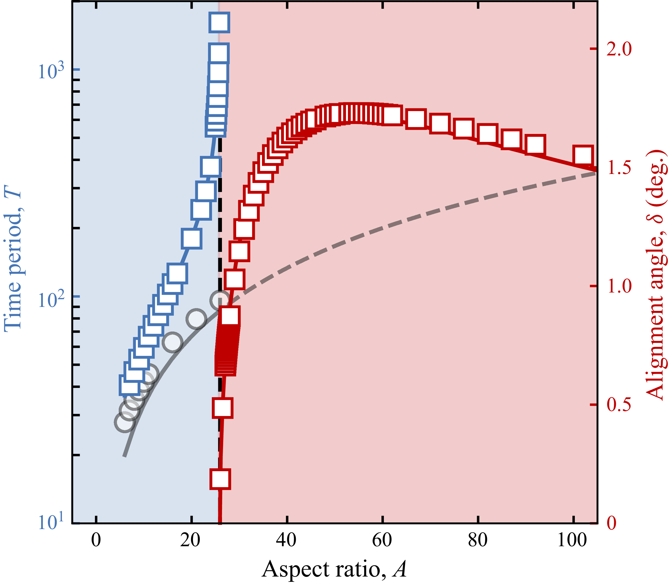


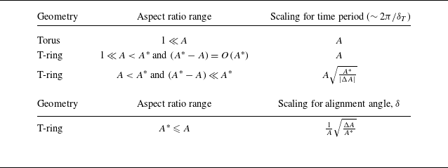


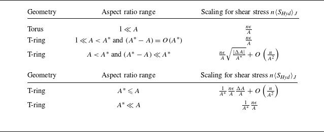


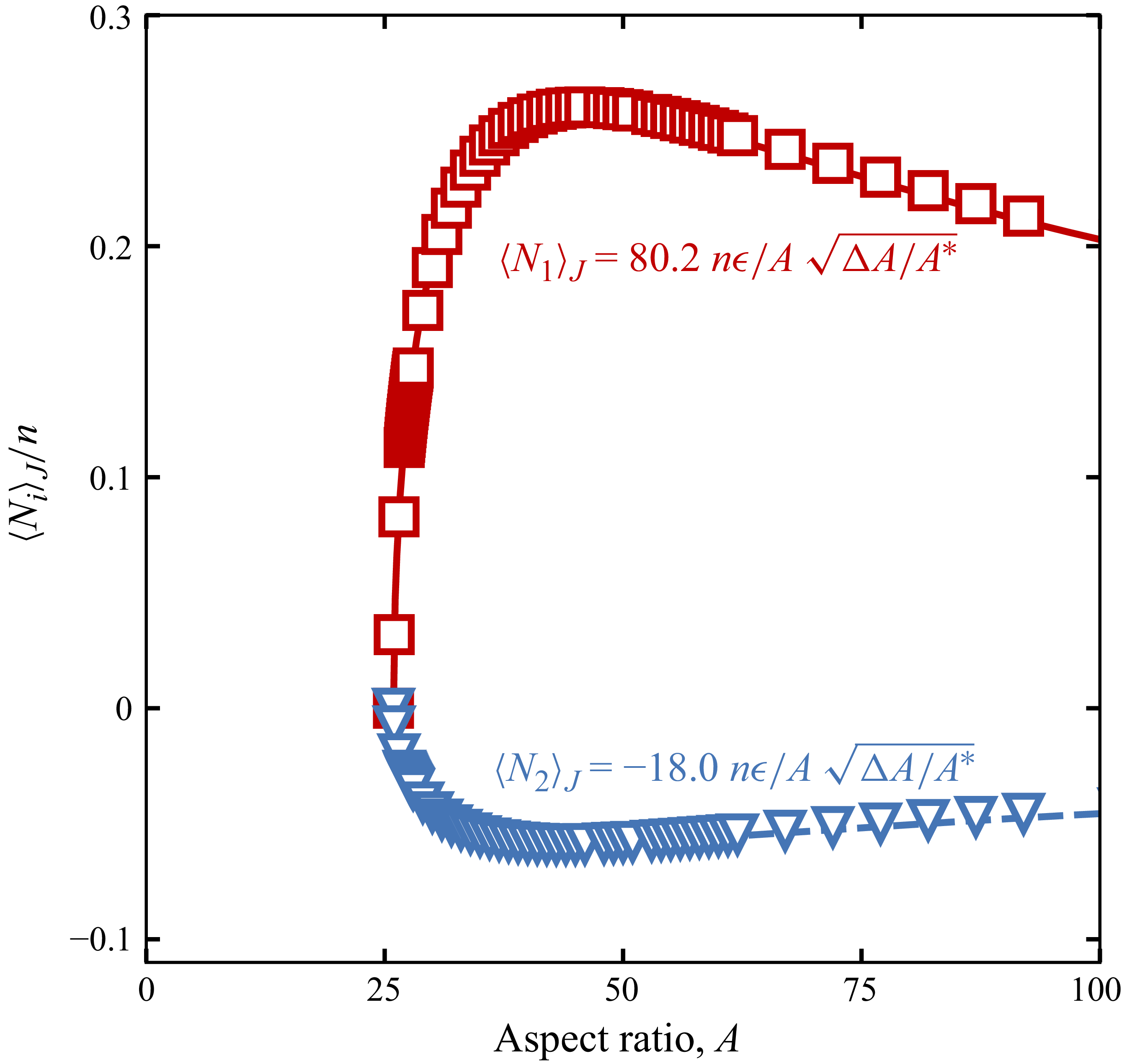


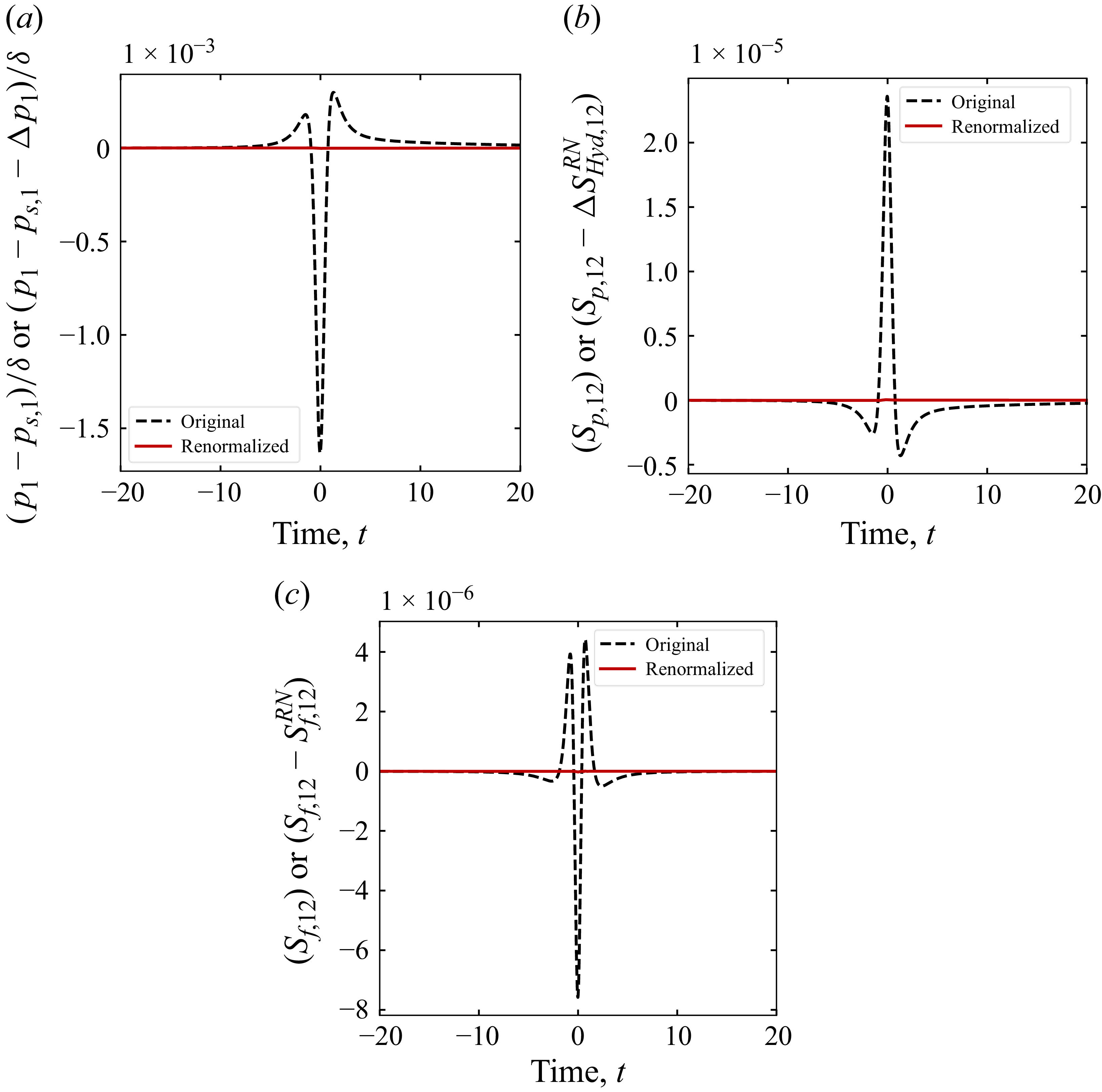


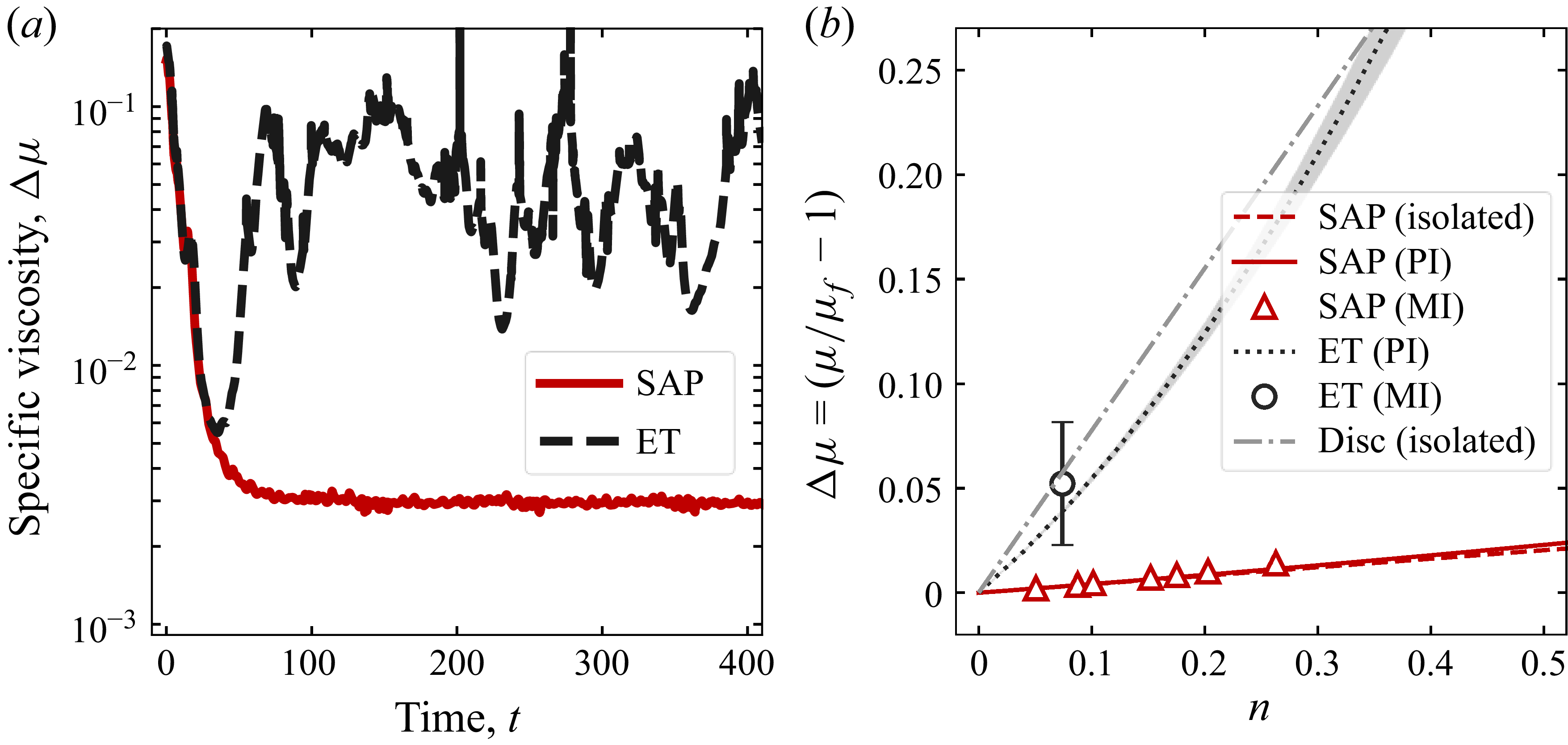


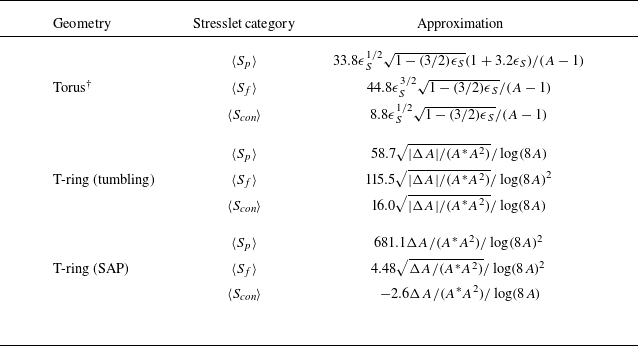


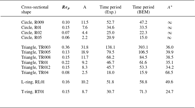


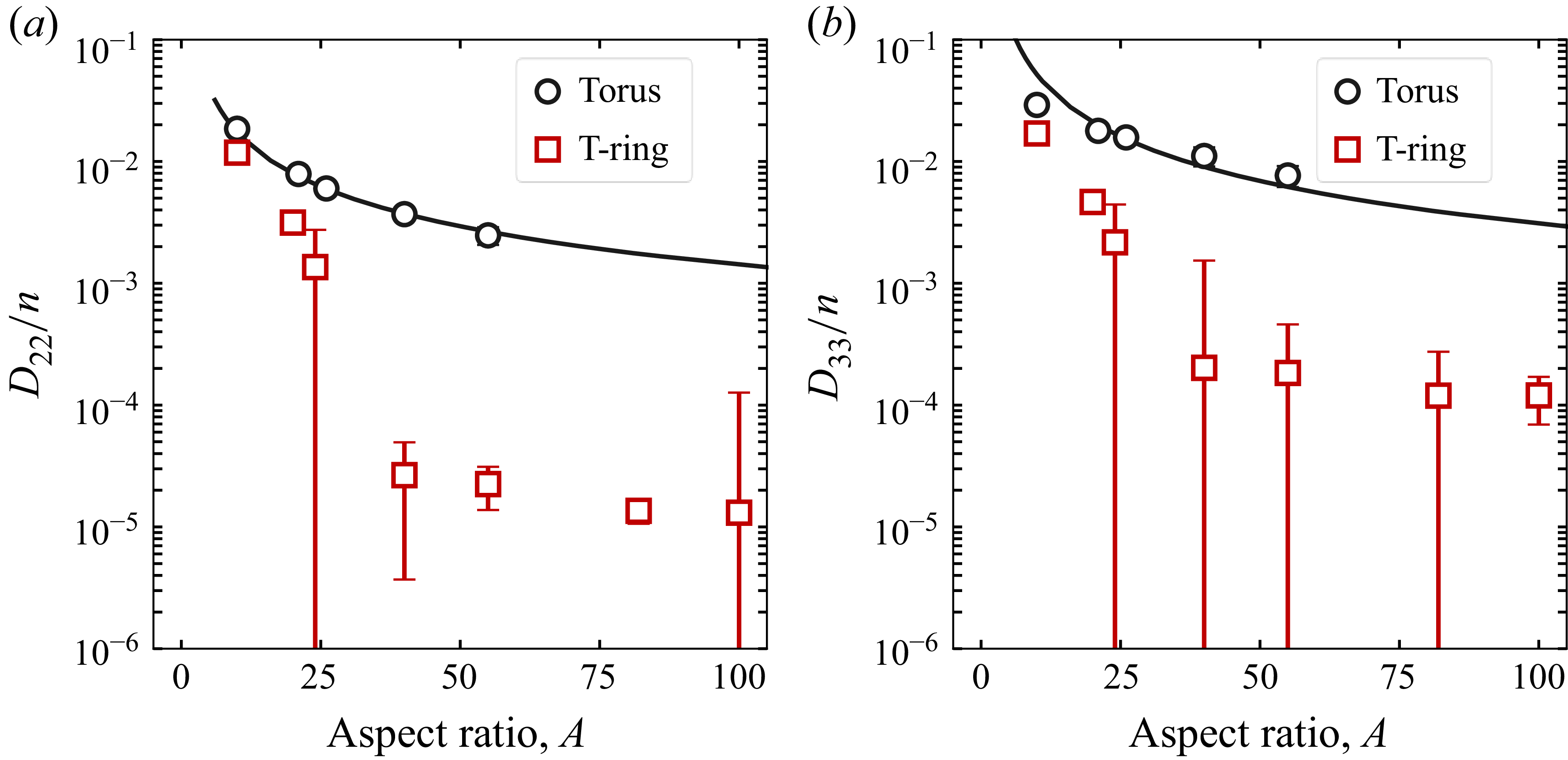


 Open access

