2. Problem formulation

Consider the gravity/buoyancy-induced motion of a 3-D deformable drop near an infinite, inclined plane solid wall under creeping flow conditions. Both the drop and external liquids are Newtonian, isothermal and free from surfactants. The drop is non-wetting, and so, it is always separated by a lubrication film from the wall due to drop motion. The wall tilt angle to horizontal is $\theta$, the non-deformed drop radius is $a$, the drop and the medium dynamic viscosities are $\mu _d$ and $\mu _e$, respectively, with the viscosity ratio $\lambda =\mu _d/ \mu _e$. 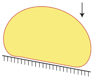Without a loss of generality, the drop is assumed to be heavier than the medium, with the density contrast $\Delta \rho >0$, and so both phases are in the upper half-space of figure 1.

Figure 1.

Schematic for drop motion on an inclined wall.

For steady-state drop sedimentation down the wall, the non-dimensional parameters are $\theta$, $\lambda$ and the Bond number

(2.1)\begin{equation} B=\frac{\Delta\rho g a^2}{\sigma}, \end{equation}

with $\sigma =\mbox {const}$ being the interface surface tension and g the standard gravity acceleration. The main goal is a rigorous study of the drop steady-state speed $U$ along the wall, the geometry of the lubrication space and the mode of drop motion in a wide range of parameters $\theta$, $\lambda$ and $B$. Specifically, we are most interested in extreme viscosity ratios $\lambda \gg 1$ and small inclination angles – the most challenging combinations that could not be approached by the more basic BI algorithms of Griggs et al. (Reference Griggs, Zinchenko and Davis2008, Reference Griggs, Zinchenko and Davis2009) and have required the development of many novel tools herein, both numerical and semi-analytical, to handle unavoidable extreme surface resolutions in dynamical simulations. The present solutions also cover a wide range of $B$ – from nearly spherical to strongly pancaked drops (but below critical for drop breakup). As in Griggs et al. (Reference Griggs, Zinchenko and Davis2008, Reference Griggs, Zinchenko and Davis2009), the drop velocity is defined as the volume average of the fluid velocity inside the drop reduced to surface integration by Gauss’ theorem, and so only the interfacial velocity has to be determined. Below, where necessary to distinguish between the transient and steady-state values for the drop speed (or other quantities), the index ‘st’ will be added to steady-state values.

A convenient, although somewhat empirical, reference velocity scale is

(2.2)\begin{equation} U_{ref}=\frac{2}{9}\frac{(\lambda+1)}{(\lambda+2/3)} \frac{\Delta\rho g a^2}{\mu_e} \sin\theta, \end{equation}

which is the steady-state speed of an isolated spherical drop under reduced gravity $g\sin \theta$. To make the equations and results below non-dimensional, all the velocities will be scaled with $U_{ref}$, lengths with $a$ and times with $a/U_{ref}$. Note that a different velocity scale, $\sigma /\mu _e$, is used in the asymptotic theory of Hodges et al. (Reference Hodges, Jensen and Rallison2004); the ratio of the two scales is $O(B\sin \theta )$. The scale (2.2) was chosen in the present work, since it makes the non-dimensional, steady-state drop speed $U$ much less sensitive to $\theta$ and $B$.

4. Numerical analysis

4.1. Validation test: a spherical drop near a vertical wall

Although the present work is largely devoted to the most challenging case of small tilt angles $\theta$, the opposite case of a drop in very close proximity to a vertical wall ($\theta =90^\circ$) serves as a non-trivial check for correctness of the present multipole-accelerated BI code. In the Stokes regime and with infinite surface tension, a spherical drop, initially placed at an arbitrary clearance $\delta _o$ from the wall, would continue settling at a constant speed and without lateral migration; the drop–wall interaction in this case is conveniently characterized by the non-dimensional correction factor $\varDelta (\lambda,\delta _0)$ to the Hadamar–Rybchinsky drag force on an isolated drop. It is of interest to explore how the present solution can approach this limiting case and predict $\varDelta (\lambda,\delta _0)$. A deformable, initially spherical drop in this situation, however, would drift away from the wall for viscosity ratios $\lambda >3.12$ (Magnaudet, Takagi & Legendre Reference Magnaudet, Takagi and Legendre2003). Since this drift disappears in the limit $B\to 0$, it was legitimate in our tests for small $B\neq 0$ to exclude this drift altogether by forcing the drop surface centroid to stay at a distance $1+\delta _0$ from the wall. That way, the long-time, steady-state (non-dimensional) drop velocity $U_{st}$ along the wall could be unambiguously attained (figure 7) for selected $\lambda =10$ and 300. It is this velocity (not the initial velocity at $t=0$ when the drop was strictly spherical) and the related drag coefficient $\varDelta = 1/U_{st}$ that must be compared with those for a drop with infinite surface tension. The reason is that, in the BI formulation (3.2), the fully developed, small curvature variation $\Delta k$ (due to the normal stress balance on the interface) is divided by the Bond number to produce an $O(1)$ effect as $B\to 0$. In contrast, the infinite surface-tension formulation (see below) is only based on the tangential stress balance, and replaces the normal stress balance by postulating the spherical shape. In this respect, comparison with the case of a non-deformable drop is also a sensitive check on correctness of drop shape perturbation in our BI simulations. The difference between $U(t=0)$ and $U_{st}$ is modest for $\lambda =300$ (figure 7b), but is more significant (almost 1.4 times) for $\lambda =10$, $\delta _o=0.005$ and $B=0.007$ (figure 7a).

Figure 7.

Transient speed of a slightly deformable drop settling along a vertical wall by the multipole-accelerated BI algorithm for (a) $\lambda =10$ and (b) $\lambda =300$. The drop starts from spherical, and its surface centroid is constrained to stay at a distance $1+\delta _0$ from the wall for the entire simulation.

Since small drop–wall clearances are of primary interest here, it would be attractive to use for comparison a highly accurate, $B=0$ bispherical (bipolar) coordinate solution for a spherical drop moving parallel to the wall, but such a solution could not be found in the literature (only the bubble case $\lambda =0$ for $\delta _o\geq 0.0453$ was handled, Meyyappan & Subramanian Reference Meyyappan and Subramanian1987). For this reason, the bispherical coordinate code of Zinchenko (Reference Zinchenko1980) for two generally unequal spherical drops with arbitrary viscosities and instantaneous velocities normal to the line of centres had to be used at a size ratio of $10^{-6}$ and viscosity of the larger drop $10^7$ times larger than the medium viscosity to accurately represent the case of one spherical drop near a solid wall. However, to overcome ill conditioning for such extreme parameters, the code of Zinchenko (Reference Zinchenko1980) had to be run in the quadruple precision mode.

In table 1, as $B\to 0$, our results by the multipole-accelerated BI code (with moderately adaptive, projective meshing and up to $N_\triangle =78\,\textrm {K}$ elements to guarantee the accuracy shown) are in excellent agreement with the $B=0$ bispherical coordinate solution; this limit is approached faster for smaller $\lambda$ and larger $\delta _o$. For $\lambda =300$ and $B=0$, our values of $\varDelta$ in table 1 are also consistent with the near-contact asymptotics

(4.1)\begin{equation} \varDelta(\infty, \delta_o)= \frac{8}{15}L+0.954 -\frac{4}{3} \frac{(L/10-0.193)^2} {(2L/5+0.371)},\quad L={-}\ln(\delta_o), \end{equation}

for a solid sphere moving with free rotation (which is the extension of the results from O'Neill & Stewartson Reference O'Neill and Stewartson1967). A different validation (for small and large deformations) of the present multipole-accelerated BI code will be demonstrated in Appendix D, including code performance benchmarks.

Table 1.

The drag force correction factor $\varDelta$ for a drop moving parallel to a plane wall; the $B\neq 0$ results are from the present multipole-accelerated, BI code, and the $B=0$ values are obtained by the bispherical coordinate code of Zinchenko (Reference Zinchenko1980).

4.2. The effect of high-order double-layer desingularization

The benefits of full double-layer BI desingularization, achieved through (3.11), are most pronounced when it is applied to simulations with modest resolutions. In figure 8 for $\lambda =30$, $\theta =15^\circ$ and $B=0.125$, all four simulations employed projective meshing with the same pattern of near-contact adaptivity (as described in § 3.3.1 and § B.1) and started from a spherical drop shape with the initial drop–wall clearance $\delta _o=0.01$ or $0.02$. The curves 1 and 2 are for high resolutions of $N_\triangle =46$ and 61 K, respectively, with full desingularization. Reliable steady state was achieved in these two runs for both the drop–wall clearance $\delta _{min}(t)$ (figure 8a) and the transient drop velocity $U(t)$ (figure 8b); the latter is graphically indistinguishable between the two runs. Numerical convergence for $\delta _{min}$ up to steady state (with $\delta _{min}^{st}\approx 0.0061{-}0.0062$) is also good, considering how sensitive this small quantity is.

Figure 8.

(a) Drop–wall clearance $\delta _{min}(t)$ and (b) transient drop speed in the simulations with $\lambda =30$, $\theta =15^\circ$ and $B=0.125$. Lines 1: $N_\triangle =46\,\textrm {K}$; 2: $N_\triangle =61\,\textrm {K}$; 3 and 4: $N_\triangle =8640$. The run for lines 3 was performed without high-order double-layer desingularization, leading to a crash at $t\approx 10$ with drop–wall overlap.

In contrast, the low-resolution run ($N_\triangle =8640$) with only leading-order subtraction in (3.11) (curves 3) crashed early due to drop–wall overlap (figure 8a), with subsequent divergence of BI iterations not allowing the simulation to proceed to steady state for the drop velocity (figure 8b). However, activating high-order desingularization for the same low resolution $N_\triangle =8640$ gives much better results (curves 4), with steady state achieved for the clearance (figure 8a) and drop velocity (figure 8b). In this run, roughly 12 % of the mesh nodes participated in the high-order desingularization (3.11) at large times. Although $\delta _{min}^{st}$ for this run is only half of the correct value, $U_{st}$ is in fair agreement with the correct result from the high-resolution simulations in figure 8(b). Note that such an improvement is achieved in a fundamental way through full BI desingularization, without attempts to impose an artificial repulsive barrier to prevent drop–wall overlap. Full desingularization is still beneficial for much higher resolutions, which is demonstrated in the next subsection.

4.3. Drop velocity: convergence analysis

Below, for the difficult combination $\lambda =60$, $\theta =7.5^\circ$, we explore the effects of discretization and solution strategies, primarily on the steady-state drop velocity $U_{st}$. It is far from obvious which of the three discretization strategies: (i) projective meshing of § 3.3.1, labelled as PR in what follows, (ii) $n_3$-based meshing (N3) of § 3.3.2 or (iii) non-adaptive meshing (NA) of § 3.3.3 to choose in each case, and the answer depends on the Bond number. In all the cases, acceptable results required very high surface resolutions only possible in dynamical simulations owing to multipole acceleration.

For $B=0.125$, with the drop exhibiting small deformation all the way to steady state, the drop speed trajectory $U(t)$ is presented in figure 9(a) for four simulations. Runs 1 and 2 employ projective meshing and started from a spherical drop shape with $\delta _o=0.01$. The steady-state meshing pattern for this $B$ is well represented by the low-resolution run in figure 3, but successful simulations of the steady-state drop speed and thin-film profile required much finer resolutions than $N_\triangle =8640$ could provide. Indeed, for runs 1 and 2 in figure 9(a) with $N_\triangle =61$ and 78 K, respectively, $U_{st}$ still differs by 2 %. To increase the resolution further, a one-time surface remeshing to $N_\triangle =138\,\textrm {K}$ was done at the end of run 2 preserving the mesh adaptivity pattern (by rebuilding the parametric mesh, as described in Appendix D), to provide the initial conditions for run 3 in figure 9(a), until a new steady-state drop velocity was reached. The difference between the $U_{st}$ values for 78 and 138 K resolutions is 1 %, indicating sufficient convergence (an additional run PR-246K done in a similar manner, but not included in figure 9(a), changed the steady-state drop speed from PR-138K by less than 0.17 %); the converged steady-state drop–wall clearance $\delta _{min}^{st}$ is 0.0034.

Figure 9.

Transient drop speed for $\lambda =60$, $\theta =7.5^\circ$, with (a) $B=0.125$, (b) $B=1$, (c) $B=2$ and (d) $B=5$, using various discretization schemes (PR, N3, NA) combined with various resolutions $N_\triangle$. In (b), run 5 (dashed line) is the repeat of run 3, but without the default high-order double-layer desingularization. In each panel, the inset shows the steady-state drop–wall configuration (side view along $x_1$) from the highest-resolution run.

To test the alternative, $n_3$-based discretization scheme of § 3.3.2, the run N3-61K (line 4) was performed with $\alpha$ therein set to 0.84, to have approximately the same near-contact adaptivity as for the other runs in figure 9(a) (judging by the same maximum-to-minimum mesh edge ratio of four at this $B$). However, the steady-state drop speed prediction by N3-61K is only half as accurate as by PR-61K. Presumably, superiority of PR discretization is due to the higher accuracy of surface integration (after desingularization) though a uniform parametric mesh on the auxiliary unit sphere, while in the N3 scheme such integration has to be done on a strongly non-uniform native mesh on the drop surface. Additional tests confirmed that projective meshing is the method of choice for all Bond numbers $B\leq 0.5$ at small tilts $\theta$.

For higher $B\ge 1$, however, projective meshing is not a robust approach, and the choice was only between the $n_3$-based (with default $\alpha =0.7$) and non-adaptive surface discretizations. At $B=1$ and this $\theta$, the steady-state adaptivity pattern for $n_3$-based meshing is well represented by the lower-resolution run in figure 4. For this $B$, an excellent agreement is observed in figure 9(b) between the runs N3-61K and N3-78K all the way to steady state, with only 0.75 % difference in the steady-state drop velocities (the additional runs N3-138K and N3-246K, not included in figure 9(b), gave indistinguishable steady-state drop speed, to within 0.1 %). The convergent steady-state drop–wall clearance is 0.0066. Compared with the case $B=0.125$ (figure 9a), the numerical convergence for $B=1$ is faster, but it still requires high surface resolutions only feasible with multipole acceleration. For the N3-46K run (line 3 in figure 9b), the steady-state drop speed is only accurate to 6 %. Although the lubrication effects are now spread on a wider near-contact area than for $B=0.125$, near-contact mesh adaptivity is still essential for accurate results. For example, run 4 in figure 9(b) with non-adaptive mesh and $N_\triangle =46$ K is not nearly as good as N3-46K. Finally, the dashed line 5 in figure 9(b) demonstrates, again, the significance of full double-layer desingularization (3.11) for small tilt angles $\theta$ even in high-resolution simulations. This run was a repeat of N3-46K, only the default full desingularization was replaced by the simple leading-order subtraction (i.e. $h_1$ set to zero); the result was a crash with drop–wall overlap and quite incorrect drop speed not reaching the steady state. Note also that the pronounced shoulder of the curves in figure 9(b) (even upon numerical convergence) is due to the artificial initial condition (spherical shape at the small gap of 0.01) and drop deformability, making the surface clearance $\delta _{min}(t)$ non-monotonic, so that it grows in a small time interval after the initial decrease. Once $\delta _{min}(t)$ resumes its regular decline, the shoulder of the curves for $U(t)$ disappears.

For $B=2$ in figure 9(c), only the simulations N3-78K and N3-138K show good convergence, with $U_{st}$ differing by 1.2 % between the two runs (further increase of $U_{st}$ in an additional run N3-246K was only 0.5 %); the steady-state drop–wall gap is 0.0064. The run N3-61K underestimates the steady-state drop speed by approximately 5 %. The cruder resolution $N_\triangle =46$ K could not give satisfactory results at all, especially with non-adaptive meshing (line 5 for NA-46K), and so $n_3$-based meshing is still a preferable discretization strategy for this $B=2$.

It was particularly difficult to obtain the correct steady-state drop speed for a strongly pancaked drop, $B=5$ (figure 9d), with imperative ultrahigh surface resolutions; also, the partially deflated form of the BI equation (3.1) (instead of fully deflated) was mostly beneficial in this case to reach numerical convergence. The steady-state pattern of non-adaptive meshing for this $B$ is well represented by the lower-resolution run in figure 5. In figure 9(d), runs NA-246K and NA-328K both reliably reached the steady state, with excellent convergence all the way (the difference in $U_{st}$ between the two runs being only 0.5 %); the steady-state drop–wall clearance is 0.0046 for NA-246K and 0.0049 for NA-328K. However, run NA-138K (curve 3) could not reach the steady state due to discretization errors and had to be stopped (it would significantly underpredict $U_{st}$ anyway). Run NA-46K (line 4) had to be stopped even sooner due to poor accuracy. Since a strongly pancaked drop on a gently inclined wall is characterized by a large near-contact spot, one could expect a meshing adaptive to that region to perform better. However, the opposite is observed, and run N3-46K (line 5) is even less successful than NA-46K. Among possible explanations for this phenomenon, it can be noted that, for a given $N_\triangle$, mesh concentration in a large near-contact area significantly depletes the node density on the rest of the drop and makes it less uniform there, thus negatively affecting the accuracy of global surface integration. Such numerical integration errors are amplified at $\lambda \gg 1$, because of the proximity of $(\lambda -1)/(\lambda +1)$ to the spectrum of the BI equation (3.1). Also, for a strongly pancaked drop, the near-contact stresses are distributed on a larger area (than for small or moderate $B$), which makes them smaller, and it may be even less important to use very fine mesh in the spot area at the expense of the outer and transition regions. Thus, non-adaptive meshing with an ultrahigh number $N_\triangle$ of elements appears to be the only successful way in this case.

5. Physical results

Figure 10(a–d), the main result of this effort, presents the non-dimensional steady-state drop speed $U$ (as defined in § 2) for small-to-moderate tilt angles $7.5^\circ \leq \theta \leq 30^\circ$ in the wide ranges of the Bond number $0.0625\leq B \leq 5$ and viscosity ratios $1\leq \lambda \leq 300$. For each data point, the relative error does not exceed 0.5 % (and is often much smaller). To this end, super-resolutions with up to $N_\triangle =328$ K had to be used for the most difficult combinations of the small tilt $\theta =7.5^\circ$ with high viscosity ratios $\lambda \ge 60$. However, the case $\theta =7.5^\circ$, $\lambda =300$, $B=5$ still could not be studied, requiring even higher resolution to avoid non-convergence of BI iterations on the way to steady state. (This difficulty did not stem from the surface curvature/normal vector calculations by the default best paraboloid-spline method employed here for all $B\geq 1$. Using instead the high-order normal vector/curvature algorithm from Appendix B of Zinchenko & Davis (Reference Zinchenko and Davis2006) for $\theta =7.5^\circ$, $\lambda =300$, $B=5$ and $N_\triangle =328$ K, the run stalled at almost the same time moment, with non-convergence of BI iterations. It remains to be seen in future work if improved schemes for surface integration could handle this case better.) On the other hand, for $\lambda =O(1)$ and moderate tilt angles $\theta \geq 22.5^\circ$, the resolution $N_\triangle =35$ K was always sufficient for high accuracy of $U$. For convenience, all the data from figure 10(a–d) are also presented in the Supplementary Material in tabular form available at https://doi.org/10.1017/jfm.2024.998.

Figure 10.

Steady-state drop speed for tilt angles (a) $\theta =7.5^\circ$, (b) $\theta =15^\circ$, (c) $\theta =22.5^\circ$ and (d) $\theta =30^\circ$. In each panel, curves (top to bottom) correspond to viscosity ratios $\lambda =1,3,10,30,60$ and $300$, respectively.

The early efforts of Griggs et al. (Reference Griggs, Zinchenko and Davis2008, Reference Griggs, Zinchenko and Davis2009) used a much simpler BI algorithm without multipole acceleration and high-order, double-layer near-singularity subtraction, and they focused on the range of tilt angles $\theta \geq 30^\circ$ and viscosity ratios $\lambda = O(1)$ to calculate the steady-state drop speed. While their resolution (up to $N_\triangle \sim 8640$) was quite acceptable in that generic range (especially in the simpler, most favourable case $\lambda =1$, see table 2), a few attempts therein to consider just slightly smaller tilts $\theta$ and/or slightly higher $\lambda$ quickly led to loss of accuracy. For example, at $\theta =15^\circ$, $B=3$ and $\lambda =1$, their solution underestimates $U$ by just 5 % (compared with the present code), but the error reaches $-$12 % for $\lambda =10$ at the same $\theta$ and $B$. In contrast, for $\lambda =20$ (the highest viscosity ratio in Griggs et al. Reference Griggs, Zinchenko and Davis2008, Reference Griggs, Zinchenko and Davis2009), $\theta =15^\circ$ and $B=4$, their solution overpredicted the drop speed by 15 %. A similar loss of accuracy is observed in the results of Griggs et al. (Reference Griggs, Zinchenko and Davis2009) for $\theta =7.5^\circ$, $\lambda =8.5$ and $0.25\leq B\leq 2$. Moreover, just slightly more extreme conditions could not be simulated at all with such algorithm and resolutions $N_\triangle \sim 8640$ due to non-convergence of BI iterations on the way to steady state. For example, simulations with $\lambda =60$, $\theta =30^\circ$ and $B=5$ failed; so did the runs with $\lambda =60$, $\theta =22.5^\circ$ and all $B\geq 2$. Simulations with $\lambda =300$ and $\theta =30^\circ$ could not succeed for any $B$ for the same reason (let alone more challenging, small tilt angles $\theta$). Thus, the present solution in figure 10(a–d) not only greatly improves the accuracy for generic values of $\theta$, $\lambda$ and $B$, but also greatly expands the parameter range owing to superhigh resolutions, feasible through multipole acceleration combined with the high-order near-singularity subtraction in the double-layer BI.

Table 2.

Non-dimensional steady-state drop speed for $\theta =30^\circ$ and $\lambda =1$. The results from figure 5(c) of Griggs et al. (Reference Griggs, Zinchenko and Davis2008) are taken with the factor of two to account for our scale (2.2).

Inclusion of $\sin \theta$ in the velocity scale (2.2) considerably mitigates the dependence of $U$ on $\theta$ (for small $B$), but $U$ is still a sharp function of the Bond number at small tilt angles (figure 10a), especially with high viscosity ratios and near the spherical drop limit. For $\theta =7.5^\circ$, $U$ is a decreasing function of $B$ in the whole range $B\geq 0.0625$ for all $\lambda \geq 1$, which is confirmed by some simulations (with $\lambda =1$, 60 or 300) extended to $B=0.0625$ (figure 10a). At a larger tilt $\theta =15^\circ$ (figure 10b), the same behaviour is observed, except for $\lambda =1$ where the trend is just starting to reverse and $U(B)$ reaches a maximum at $B\approx 0.15$; high accuracy of our simulations (especially at $\lambda =1$) gives confidence that this trend reversal is not a numerical effect. For $\theta =22.5^\circ$ (figure 10c) and $\lambda =1$, this maximum of $U(B)$ becomes more noticeable; also, the trend reversal is seen to emerge at $\lambda =60$ while $U(B)$ remains monotonic to $B=0.0625$ for the higher viscosity ratio of 300. Finally, at the tilt angle of $30^\circ$ (figure 10d) and $\lambda =1$, the maximum of $U(B)$ is most pronounced, shifting to a higher Bond number $B\approx 0.5$; the $\lambda =60$ curve also shows a (very weak) maximum at $B\approx 0.1$, but the trend reversal is still not seen to $B=0.0625$ for $\lambda =300$. Note that Griggs et al. (Reference Griggs, Zinchenko and Davis2009) also observed weakly non-monotonic behaviour of $U(B)$ at $\theta =30^\circ$ and $\lambda \approx 1$, in both their experiments and simulations (table 2).

In their analytical study, Hodges et al. (Reference Hodges, Jensen and Rallison2004) identified 11 asymptotic regimes for a non-wetting drop sedimenting on a gently inclined wall, to give leading-order estimates for the steady-state drop velocity and thin-film thickness depending on the relations between $\theta$, $\lambda$ and $B$. Their analysis naturally assumes logarithmically very broad variation of these parameters; the boundaries on different asymptotic regions are very tight, unless the tilt $\theta$ can be made extremely small (which was not possible in the present simulations). For strongly pancaked drops $B=5$ at $\theta =7.5^\circ$ and moderate viscosity ratios $\lambda =10{-}30$, an approximate agreement between our precise drop-speed results and the asymptotic theory predictions (region $\mbox {PII}_1$ in Hodges et al. Reference Hodges, Jensen and Rallison2004) was observed, although the difference could reach 1.5 times. With this exception, even though the present solution greatly expands the parameter space compared with Griggs et al. (Reference Griggs, Zinchenko and Davis2008, Reference Griggs, Zinchenko and Davis2009), it was still hardly possible to make quantitative connections with the asymptotic theory of Hodges et al. (Reference Hodges, Jensen and Rallison2004). For $B\ll 1$, one source of such difficulties is obvious from our figure 10. According to Hodges et al. (Reference Hodges, Jensen and Rallison2004), as $B\to 0$ for fixed $\theta$ and $\lambda$, our $U(B)$ must approach zero, albeit slowly like ${\sim }|\ln (\theta ^2 B)|^{-1}$ (note the difference in the definitions of the non-dimensional drop speed $U$ between the present work and their work). Even at $\theta =30^\circ$ and $\lambda =1$, it would require extremely small $B$ (well past the reversal trend for $U(B)$ in figure 10d) to observe a substantial decrease of the drop speed, let alone smaller tilt angles and/or higher viscosity ratios. Such Bond numbers are computationally not feasible and would correspond to extremely small drop–wall clearance (see below), where surface roughness and other small-scale effects can come into play in practice.

Qualitatively, our trend reversal for $U(B)$ can be explained by the theory of Hodges et al. (Reference Hodges, Jensen and Rallison2004). Namely, before reaching zero as $B\to 0$, $U(B)$ must first go through either $\mbox {FIII}_1$ or $\mbox {FIII}_2$ asymptotic regions of the map in their figure 12, with the scalings $U(B)\sim B^{-1/4}\theta ^{1/2}$ in both regions. Quantitatively, however, the asymptotics of Hodges et al. (Reference Hodges, Jensen and Rallison2004) for these regions do not describe the well-tested results in our figure 10 at small $B$. One reason may be the neglect (in theory) of rim-edge energy dissipation, which scales (for $B\ll 1$) like $1.4B^{-1/5}(Ca)^{2/15}$ relative to the total dissipation elsewhere in the rim (Hodges et al. Reference Hodges, Jensen and Rallison2004); here, $Ca=\mu _e U_{dim}/\sigma$ is the capillary number based on the dimensional drop speed $U_{dim}$; this ratio must be small for the asymptotic theory to be applicable. However, based on our drop-speed results (figure 10), this ratio is approximately unity for all small $B$. (By a similar analysis, pancaked drops $B\sim 5$ are only slightly more favourable for the neglect of rim-edge dissipation.)

It was possible, however, to make comparisons with the experimental work of Rahman & Waghmare (Reference Rahman and Waghmare2018) who measured the steady-state drop speed on a tilted glass plane submerged in a different liquid with viscosity ratio $\lambda =0.1$, $10$ or $110$ at very small Bond numbers. No sticking threshold was reported, and so their data presumably do not suffer from the contact angle hysteresis and correspond to the present model of a non-wetting drop. For $\lambda \geq 10$, $\theta \leq 15^\circ$ and $B\leq 0.04$, the dimensional drop speed $U_{dim}$ was fitted in Rahman & Waghmare (Reference Rahman and Waghmare2018) by a semi-empirical relation

(5.1)\begin{equation} U_{dim}\sim \frac{B\sigma\sin\theta}{\mu_d B^{3/2}+6{\rm \pi}\mu_e}\end{equation}

(although it is difficult to judge how accurately this fit represents their data since their dimensional speed covers a very broad range represented logarithmically). Using our velocity scale (2.2) to make (5.1) non-dimensional, comparison was made with our precise results in figure 10 for all pairs with $\theta \leq 15^\circ$, $\lambda \geq 10$ and $B\leq 0.125$ (table 3). In most cases, there is only a modest difference, although, in a few instances (with $\theta =7.5^\circ$ and large $\lambda \geq 30$), (5.1) overpredicts our $U$ by 38 %–42 %. This equation does not capture the non-monotonic behaviour of our $U(B)$ in figure 10 and quickly becomes inadequate with the increase in the Bond number. Again, the lack of simulation data for $B\ll 0.0625$ did not allow for more representative comparisons with the experiments of Rahman & Waghmare (Reference Rahman and Waghmare2018).

Table 3.

Comparison of the non-dimensional steady-state drop speed $U$ from the present simulations with the semi-empirical formula of Rahman & Waghmare (Reference Rahman and Waghmare2018). For each set of $\theta$, $B$ and $\lambda$, the upper value is from our figure 10; the lower value is from (5.1) scaled on (2.2).

Another difficulty with connecting our work to Hodges et al. (Reference Hodges, Jensen and Rallison2004) is that their 3-D thin-film thickness is characterized by a single parameter $\epsilon$, while we pursue a more complete description of the dimple observed in the present simulations (as well as in those of Griggs et al. Reference Griggs, Zinchenko and Davis2008, Reference Griggs, Zinchenko and Davis2009); this dimple very slowly disappears as $B\to 0$. Instead of the topographic maps (Griggs et al. Reference Griggs, Zinchenko and Davis2008, Reference Griggs, Zinchenko and Davis2009) for the film profile, we use here a more compact dimple characterization in steady state by three parameters, $\delta _{min}$, $\delta _{av}$ and $\delta _{max}$. The first one (already used in § 4.2) is the global minimum of the mesh node-to-wall distances, while $\delta _{av}$ and $\delta _{max}$ are, respectively, the surface average and maximum of such distances calculated in the dimple region only. This region is unambiguously defined as the set of drop-mesh nodes where at least one of the principal surface curvatures $k_1$ or $k_2$ is negative. Obviously, such definition makes sense for small tilt angles, when the drop is in near contact with the wall; note that $\delta _{min}$ is reached very slightly outside the rim of the so-defined dimple.

These three metrics, $\delta _{min}$, $\delta _{av}$ and $\delta _{max}$ (all well convergent with respect to resolutions) are presented in figure 11 for $\theta =7.5^\circ$ (a–c) and $15^\circ$ (d–f). In each panel, red squares are for $\lambda =1$, green circles for $\lambda =60$ and black diamonds for $\lambda =300$. For small $B$, each quantity in figure 11(a–c) approximately obeys the scaling ${\sim }B^{1/2}\sin \theta$, in qualitative agreement with the asymptotic analysis of Hodges et al. (Reference Hodges, Jensen and Rallison2004), although this scaling is likely not the ultimate one for $B\to 0$, since their theoretical estimate also includes a logarithmically weak factor of $O(|\ln (\theta ^2 B)|^{-1})$ (without the after-log term). However, the above scaling fits our $B\ll 1$ results in figure 11(a–c) with numerical factors almost independent of $\lambda =1{-}300$, but sensitive to the choice of the metric (namely, the factor is within 0.07–0.076 for $\delta _{min}$, and 0.13–0.14 for $\delta _{max}$). The asymptotic theory does not discern such thin-film details sufficiently for comparison with our simulations (in particular, $\delta _{min}$ is not resolved in the theory).

Figure 11.

Steady-state thin-film metrics (a,d) $\delta _{min}$, (b,e) $\delta _{av}$ and (c, f) $\delta _{max}$ vs Bond number for (a–c) $\theta =7.5^\circ$ and (d–f) $\theta =15^\circ$. Red squares: $\lambda =1$, green circles: $\lambda =60$, black diamonds: $\lambda =300$.

For a pancaked drop $B\geq O(1)$, the geometry of the lubrication space becomes strongly sensitive to the viscosity ratio. While the film thickness saturates with the increase in the Bond number to $B\approx 1{-}2$ for a highly viscous drop $\lambda =60$, it continues to grow for $\lambda =1$, at least in the range $B\leq 5$, thus making the film much thicker for a homoviscous drop compared with a drop with high viscosity ratio. This observation is confirmed for all the metrics in figure 11(a–c).

For a larger tilt $\theta =15^\circ$ and high viscosity ratios, only $\delta _{min}$ saturates with the increase in the Bond number (figure 11d), while the two other thin-film metrics continue to grow monotonically with $B$ (figure 11e, f); the film is still thicker for a homoviscous drop than for a drop with $\lambda \geq 60$. Comparison between (a–c) and (d–f) shows that a linear scaling of the film thickness parameters with the tilt angle $\theta$ or $\sin \theta$ roughly holds for $\delta _{av}$ and $\delta _{max}$ in case of highly viscous drops, and for all three metrics in case of homoviscous drops. However, significant deviations from this scaling are observed for $\delta _{min}$ in case of highly viscous pancaked drops.

The asymptotic lubrication analysis of Hodges et al. (Reference Hodges, Jensen and Rallison2004) for $\theta \ll 1$ predicts, to the leading order, uniform film thickness $\delta$ from the back to the front of the film, i.e. in the notations of our figure 1, $\delta$ must be only a function of $x_1$. To verify this prediction, $\delta$ was computed for $\theta =7.5^\circ$ on the central cross-section of the dimple region (i.e. in the $(x_2, x_3)$-plane drawn through the drop centroid $\boldsymbol {x}^c$) and plotted vs $x_2 -x_2^c$. (Some lack of smoothness in figure 12 may be due to presentation, with the simplest, zero-order interpolation from the 3-D mesh of triangles to the central plane.) For a pancaked drop $B=2$ (figure 12a), $\delta$ is indeed practically constant in the dimple cross-section, except for the narrow range of $x_2-x_2^c$ at the tail where the film is substantially thinner. This behaviour is observed for $\lambda =1$, 60 and especially for 300. Note that the global minimum of $\delta$ for each of these $\lambda$ is not approached in figure 12(a); it is significantly smaller (see figures 11(a) and 13(a)) and reached well outside the central plane $(x_2, x_3)$, so that $\delta$ remains a strong function of $x_1$. For a slightly deformable drop $B=0.0625$ (figure 12b), however, even film uniformity along the drop motion direction cannot be assumed as an approximation; here, a large portion of the film cross-section (near the tail) is much thinner than the rest of the film in the $(x_2, x_3)$-plane and does not approach a constant thickness as $x_2$ grows.

Figure 12.

Profile of the steady-state thin-film thickness in the central cross-section of the dimple region for $\theta =7.5^\circ$. Panels show (a) $B=2$; (b) $B=0.0625$. Lines 1: $\lambda =1$, 2: $\lambda =60$, 3: $\lambda =300$.

Figure 13.

Contour plots of the steady-state thin-film thickness $\delta (x_1,x_2)$ in the near-contact spot for $\theta =7.5^\circ$ and $\lambda =300$. (a) $B=2$; (b) $B=0.0625$. View from the drop bottom. In (a), the outer boundary shows the entire drop projection on the $(x_1,x_2)$-plane. The minimum clearance $\delta _{min}$ is 0.0049 for (a) and 0.00248 for (b).

The lubrication space geometry in the entire near-contact spot is also much different between the $B=2$ and $B=0.0625$ cases, as demonstrated in figure 13 for $\lambda =300$. While the contour lines for drop–wall clearance in figure 13(a) tend to be parallel to the $x_2$-axis, there is no such region at $B=0.0625$ in figure 13(b). On the other hand, the distribution of $\delta$ in the trailing part of the spot resembles axisymmetric for $B=0.0625$ – a feature absent for $B=2$. These observations additionally explain particular difficulties of comparison with the asymptotic theories for $B\ll 1$, requiring much smaller $\theta$ and $B$ than possible in rigorous simulations.

Finally, all the results in figures 11 and 12 indicate that a non-uniform 3-D film profile with finite thickness is approached, albeit slowly, for every fixed $\theta$ and $B$, as $\lambda \to \infty$. This last observation is in line with the arguments of Hodges et al. (Reference Hodges, Jensen and Rallison2004) that the steady-state, high viscosity ratio limit must correspond to pure drop sliding as a rigid body, since tumbling is prohibited by the drop non-sphericity. It can be added to their arguments that the lack of fore–aft symmetry of the drop shape developing in this limit explains how such mode of the drop motion is possible at all at zero Reynolds number. A solid sphere moving parallel to the wall would only experience a lateral hydrodynamic force, not capable to counter the gravity effect and maintain a steady-state film thickness. More generally, lateral translation of a non-spherical solid particle with fore–aft symmetry would not produce a normal hydrodynamic force either (as follows from the reciprocal theorem) necessary for the particle to glide, and so a loss of such symmetry is crucial to maintain a steady-state regime.

Besides sliding, Hodges et al. (Reference Hodges, Jensen and Rallison2004) also classify other possible steady-state kinematics for a drop motion down an inclined wall. One of them is tank treading for a pancaked drop, where the circulation fluid velocity inside the drop is comparable in magnitude to the drop speed, and is uniform over the near-contact spot. The other regime is rolling of a nearly spherical drop, with rigid-body rotational motion comparable in magnitude to the drop speed. It is of interest to see if the present simulations for $\lambda \gg 1$ and small tilt angles fall, at least qualitatively, into any of these regimes.

To this end, the fluid circulation velocity $\boldsymbol {u}-\boldsymbol {U}$ was computed along the central cross-section of the whole drop surface (i.e. in the $(x_2, x_3)$-plane drawn through the drop centroid) and presented in figure 14(a–l) for different combinations of $\lambda$, $\theta$ and $B$. For each combination, a reference vector (placed inside the drop) represents the steady-state drop velocity $\boldsymbol {U}$. For each field vector, its length relative to the length of the reference vector gives the local circulation intensity ${\mathcal {C}}= \|\boldsymbol {u}-\boldsymbol {U}\|/U$ at the starting surface point of the field vector. The maximum and minimum values of ${\mathcal {C}}$ over the entire cross-section contour are also listed for each set of $\lambda$, $\theta$ and $B$; the maximum is reached in the near-contact spot close to the trailing edge, while the minimum is observed just in front of the spot. The global drop shape in figure 14 is a strong function of $B$, but is almost insensitive to $\lambda$ and $\theta$, since it is close (for small tilts) to the hydrostatic equilibrium shape on a horizontal plane unaffected at all by the viscosity ratio (e.g. Hodges et al. Reference Hodges, Jensen and Rallison2004).

Figure 14.

Steady-state circulation velocity $\boldsymbol {u}-\boldsymbol {U}$ along the central cross-section of the drop surface. Length of each field vector on a contour relative to the length of the reference vector (inside this contour) gives local circulation intensity ${\mathcal {C}}= \|\boldsymbol {u}-\boldsymbol {U}\|/U$.

However, $\lambda$ and $\theta$ have a strong effect on the circulation intensity ${\mathcal {C}}$. For a pancake drop $B=2$ and tilt $\theta =15^\circ$, the sliding regime is quickly approached as $\lambda$ is increased from 60 to 300: in figure 14(b), the circulation intensity is within 5 % on the whole drop contour, which is an almost perfect sliding regime, while the $\lambda =60$ motion (a) is better described as tank treading (with large slip at the wall). Decreasing the Bond number to 0.5 (c,d) enhances the circulation, especially for $\lambda =300$, but the kinematics in (d) is still close to sliding, judging by the small values of ${\mathcal {C}}$. For an even smaller $B=0.0625$ in (e, f), only the vicinity of the near-contact spot is shown; the rest of the drop is nearly spherical, with nearly constant ${\mathcal {C}}\approx {\mathcal {C}}_{min}$. A marked difference between (e, f) is much more uniform circulation for $\lambda =300$, and so the kinematics in ( f) is best described as rolling with sliding; the circulation here does not exceed 27 %.

At the smaller tilt $\theta =7.5^\circ$ (g–l), convergence to the pure sliding regime $\lambda =\infty$ is much slower and would require much larger values of the viscosity ratio; in (h) for $\lambda =300$ and $B=2$, the circulation intensity still reaches 11 % (cf with (b)). Again, for the smallest $B=0.0625$, increasing $\lambda$ from 60 (k) to 300 results in a much more uniform circulation, so that the kinematics in (l) resembles rolling with sliding; the value of ${\mathcal {C}}_{max}=0.35$ is still away from unity. It appears that for liquid–liquid systems in a purely hydrodynamical formulation, with a smooth solid wall and in the absence of singular adhesive forces, the thin-film lubrication can never provide for perfect rolling (i.e. ${\mathcal {C}}\approx 1$).

It is not obvious from figure 10 how our results could be used to accurately predict the drop speed for an arbitrary viscosity ratio from 1 to 300, or in a wider range $\lambda >300$. In this respect, it was found helpful (mostly for moderate-to-large Bond numbers) to plot $U(\lambda +1)/(\lambda +2/3)$ vs $\lambda ^{-1/3}$ (figure 15). For $B=1$, $2$ and $5$, and all tilt angles from $7.5^\circ$ to $30^\circ$, a smooth dependence on $\lambda ^{-1/3}$ is observed, allowing for accurate interpolation to an arbitrary $\lambda \in (1,300)$. Moreover, at the small tilt of $7.5^\circ$, the results are almost linear with $\lambda ^{-1/3}$ to $\lambda =300$, allowing for reasonably credible predictions of the drop speed to $\lambda \approx 1000$ by extrapolation. Theoretical explanation of such, almost linear, behaviour in a wide range of $\lambda$ is lacking and it is, obviously, not the ultimate behaviour for $\lambda \to \infty$. Indeed, for fixed $B$ and $\theta$, the finite-$\lambda$ correction to the drop speed must be asymptotically $O(\lambda ^{-1})$ (since it would become a problem of regular perturbation). This change of behaviour is seen most vividly for the moderate tilt of $30^\circ$ (figure 15d), where the convergence to the sliding limit $\lambda =\infty$ is much faster for $B=5$ than for $B=1$ due to larger drop–wall separation in the former case. Again, a qualitative connection is seen with the work of Hodges et al. (Reference Hodges, Jensen and Rallison2004): from their figure 12, the sliding regime requires $\lambda \gg (B^{1/2}\sin ^2 \theta )^{-1}$, i.e. smaller viscosity ratios as the Bond number and/or the tilt angle are increased.

Figure 15.

Steady-state values of $U(\lambda +1)/(\lambda +2/3)$ for (a) $\theta =7.5^\circ$, (b) $\theta =15^\circ$, (c) $\theta =22.5^\circ$ and (d) $\theta =30^\circ$. Curves (top to bottom) are for $B=1$, $2$ and $5$, respectively.

It would be interesting, albeit challenging, to have special simulation or semi-analytical methods for the sliding limit $\lambda =\infty$. One difficulty is that the relevant solid-body shape with a dimple and wide near-contact spot is unknown a priori and must be a part of the solution. Also, the available asymptotic approach to handle close hydrodynamical interaction of a non-spherical solid particle with a wall or another particle (Cox Reference Cox1974; Claeys & Brady Reference Claeys and Brady1989; Staben, Zinchenko & Davis Reference Staben, Zinchenko and Davis2006) is based on lubrication analysis at the single point of near contact and would not be applicable in the present case.