







1. Introduction
The Navier–Stokes equations (NSE) are dissipative partial differential equations (PDE) that describe the motion of fluid flows. When they have complex dynamics, their description requires a large number of degrees of freedom – a high state-space dimension – to accurately resolve their dynamics. However, due to the fast damping of small scales by viscous diffusion, the long-time dynamics relaxes to a finite-dimensional surface in state space, an invariant manifold  $\mathcal{M}$ of embedding dimension $d_{\mathcal{M} }$ (Foias, Manley & Temam Reference Foias, Manley and Temam1988; Temam Reference Temam1989; Zelik Reference Zelik2022). The long-time dynamics on $\mathcal {M}$ follows a set of ordinary differential equations (ODE) in $d_\mathcal {M}$ dimensions; since $\mathcal {M}$ is invariant under the dynamics, the vector field defined on $\mathcal {M}$ remains tangential to $\mathcal {M}$. Classical data-driven methods for dimension reduction, such as proper orthogonal decomposition (POD), approximate this manifold as a flat surface, but for complex flows, this linear approximation is severely limited (Holmes et al. Reference Holmes, Lumley, Berkooz and Rowley2012). Deep neural networks have been used to discover the global invariant manifold coordinates for complex chaotic systems such as the Kuramoto–Sivashinsky equation, channel flow, Kolmogorov flow or turbulent planar Couette flow (Milano & Koumoutsakos Reference Milano and Koumoutsakos2002; Linot & Graham Reference Linot and Graham2020; Page, Brenner & Kerswell Reference Page, Brenner and Kerswell2021; Linot & Graham Reference Linot and Graham2023; Pérez De Jesús & Graham Reference Pérez De Jesús and Graham2023; Zeng & Graham Reference Zeng and Graham2023). Floryan & Graham (Reference Floryan and Graham2022) recently introduced an approach in which the global manifold is split into local charts to identify the intrinsic dimensionality of the manifold (i.e. minimal-dimensional representation of a manifold often necessitates multiple local charts). This approach is natural for dealing with discrete symmetries, as illustrated in Pérez-De-Jesús, Linot & Graham (Reference Pérez-De-Jesús, Linot and Graham2023). In the present work, we only consider global coordinates in the embedding dimension of the manifold.
Turbulent flows exhibit patterns that persist in space and time, often called coherent structures (Waleffe Reference Waleffe2001; Kawahara, Uhlmann & van Veen Reference Kawahara, Uhlmann and van Veen2012; Graham & Floryan Reference Graham and Floryan2021). In some cases, non-turbulent exact solutions to the NSE exist that closely resemble these structures; these have been referred to as exact coherent structures (ECS). There are several ECS types: steady or equilibrium solutions, periodic orbits, travelling waves and relative periodic orbits. The dynamical point of view of turbulence describes turbulence as a state space populated with simple invariant solutions whose stable and unstable manifolds form a framework that guides the trajectory of turbulent flow as it transitions between the neighbourhoods of different solutions. Thus, these simple invariant solutions can be used to reproduce statistical quantities of the spatio-temporally-chaotic systems. This idea has driven great scientific interest in finding ECS for Couette, pipe and Kolmogorov flows (Nagata Reference Nagata1990; Waleffe Reference Waleffe2001; Wedin & Kerswell Reference Wedin and Kerswell2004; Li, Xi & Graham Reference Li, Xi and Graham2006; Page & Kerswell Reference Page and Kerswell2020).
Our aim in the present work is to apply data-driven modelling methods for time evolution of exact coherent states on the invariant manifolds where they lie. Consider first full-state data  ${\boldsymbol {x}}$ that live in an N-dimensional ambient space $\mathbb {R}^N$, where ${\rm d}\kern0.06em {\boldsymbol {x}}/{\rm d}t={\boldsymbol {f}}({\boldsymbol {x}})$ governs the evolution of this state over time. When ${\boldsymbol {x}}$ is mapped into the coordinates of an invariant manifold, denoted ${\boldsymbol {h}} \in \mathbb {R}^{d_\mathcal {M}}$, a corresponding evolution equation in these coordinates can be formulated: ${\rm d}{\boldsymbol {h}}/{\rm d}t={\boldsymbol {g}}({\boldsymbol {h}})$. To learn this equation of evolution either a state-space or function-space approach can be applied; we introduce these here and provide further details in § 2. The learning goal of the state-space modelling focuses on finding an accurate representation of ${\boldsymbol {g}}$. A popular method for low-dimensional systems when data ${\rm d}{\boldsymbol {h}}/{\rm d}t$ is available is the sparse identification of nonlinear dynamics (SINDy) (Brunton, Proctor & Kutz Reference Brunton, Proctor and Kutz2016); SINDy uses sparse regression on a dictionary of terms representing the vector field, and has been widely applied to systems where these have simple structures. A more general framework, known as neural ODE (NODE) (Chen et al. Reference Chen, Rubanova, Bettencourt and Duvenaud2019), represents the vector field $\boldsymbol {g}$ as a neural network and does not require data on time derivatives. It has been applied to complex chaotic systems (Linot & Graham Reference Linot and Graham2022, Reference Linot and Graham2023) and will be used here. Function-space modelling is based on the Koopman operator, a linear infinite-dimensional operator that evolves observables of the state space forward in time (Koopman Reference Koopman1931; Lasota & Mackey Reference Lasota and Mackey1994). To approximate the Koopman operator, a leading method is the dynamic mode decomposition (DMD) which considers the state as the only observable, making it essentially a linear state-space model (Rowley et al. Reference Rowley, Mezic, Bagheri, Schlatter and Henningson2009; Schmid Reference Schmid2010). Other methods have been proposed to lift the state into a higher-dimensional feature space, such as the extended DMD (EDMD) that uses a dictionary of observables where the dictionary is chosen to be Hermite or Legendre polynomial functions of the state (Williams, Kevrekidis & Rowley Reference Williams, Kevrekidis and Rowley2014). However, without knowledge of the underlying dynamics, it is difficult to choose a good set of dictionary elements, and data-driven approaches have emerged for learning Koopman embeddings (Lusch, Kutz & Brunton Reference Lusch, Kutz and Brunton2018; Kaiser, Kutz & Brunton Reference Kaiser, Kutz and Brunton2021). One of these approaches is EDMD with dictionary learning (EDMD-DL), in which neural networks are trained as dictionaries to map the state to a set of observables, which are evolved forward with a linear operator (Li et al. Reference Li, Dietrich, Bollt and Kevrekidis2017; Constante-Amores, Linot & Graham Reference Constante-Amores, Linot and Graham2024). In this work we are applying the Koopman operator theory to the inertial manifold theory. Nakao & Mezic (Reference Nakao and Mezic2020) and Mezic (Reference Mezic2020) showed that inertial manifolds correspond to joint zero-level sets of Koopman eigenfunctions. We also note that the Koopman theory has been applied to systems with continuous spectrum, see Arbabi & Mezić (Reference Arbabi and Mezić2017) and Colbrook, Ayton & Szöke (Reference Colbrook, Ayton and Szöke2023).
In this work, we address data-driven modelling from a dynamical system perspective. We show that both state-space and function-space approaches are highly effective when coupled with dimension reduction for exact coherent states of the NSE for Kolmogorov flow and pipe flow. The rest of this article is organised as follows: § 2 presents the framework of our methodology. Section 3 provides a discussion of the results, and concluding remarks are summarised in § 4.
2. Framework
Here we describe the framework to identify the intrinsic manifold dimension  $d_\mathcal {M}$, the mapping between $\mathcal {M}$ and the full state spaces, and learn the time-evolution model for the dynamics in $\mathcal {M}$. See figure 1 for a schematic representation. We assume that our data comes in the form of snapshots, each representing the full state from a long time series obtained through a fully resolved direct numerical simulation. With the full space, we use a recently developed IRMAE-WD (implicit rank-minimising autoencoder-weight decay) autoencoder architecture (Zeng & Graham Reference Zeng and Graham2023) to identify the mapping into the manifold coordinates ${\boldsymbol {h}}=\boldsymbol { \chi }(\tilde {\boldsymbol {x}})$, along with a mapping back $\tilde {\boldsymbol {x}}=\tilde {\boldsymbol {\chi }}({\boldsymbol {h}})$, so these functions can in principle reconstruct the state (i.e. ${\boldsymbol {x}} =\tilde {\boldsymbol {x}}$). The autoencoder is formed by standard nonlinear encoder and decoder networks denoted $\mathcal{E}$ and $\mathcal{D}$, respectively, with $n$ additional linear layers with weight matrices $W_1, W_2,\ldots, W_n$ (of size $d_z \times d_z$) signified by $\mathcal {W}_n$ in figure 1 between them (see table 1 for the architectures of the networks used in this work). The encoder finds a compact representation ${\boldsymbol {z}} \in \mathbb {R}^{d_z}$, and the decoder performs the inverse operation. The additional linear layers promote minimisation of the rank of the data covariance in the latent representation, precisely aligning with the dimension of the underlying manifold. Post-training, a singular value decomposition (SVD) is applied to the covariance matrix of the latent data matrix ${\boldsymbol {z}}$ yielding matrices of singular vectors $\boldsymbol{\mathsf{U}}$, and singular values $\boldsymbol{\mathsf{S}}$. Then, we can recast $\boldsymbol {z}$ in the orthogonal basis given by the columns of $\boldsymbol{\mathsf{U}}$ by defining ${\boldsymbol {h}}^\times =\boldsymbol{\mathsf{U}}^T {\boldsymbol {z}} \in \mathbb {R}^{d_z}$, in which each coordinate of ${\boldsymbol {h}}^\times$ is ordered by contribution. This framework reveals the manifold dimension $d_\mathcal{M}$ as the number of significant singular values, indicating that a coordinate representation exists in which the data spans $d_\mathcal {M}$ directions. Thus, the encoded data avoids spanning directions associated with nearly zero singular values (i.e. $\boldsymbol{\mathsf{U}} \boldsymbol{\mathsf{U}}^T {\boldsymbol {z}} \approx \hat {\boldsymbol{\mathsf{U}}} \hat {\boldsymbol{\mathsf{U}}}^T {\boldsymbol {z}}$, where $\hat {\boldsymbol{\mathsf{U}}}$ are the singular vectors truncated corresponding to singular values that are not nearly zero). Leveraging this insight, we extract a minimal, orthogonal coordinate system by projecting ${\boldsymbol {z}}$ onto the range of $\hat {\boldsymbol{\mathsf{U}}}$, resulting in a minimal representation ${\boldsymbol {h}} =\hat {\boldsymbol{\mathsf{U}}}^T {\boldsymbol {z}} \in \mathbb {R}^{d_{\mathcal {M}}}$. In summary, $\chi$ is defined by $\chi ({\boldsymbol {x}}) = \hat {\boldsymbol{\mathsf{U}}}^T (\mathcal {W}_n(\mathcal {E}({\boldsymbol {x}})))$, while $\tilde {\chi }({\boldsymbol {h}}) = \mathcal {D}(\hat {\boldsymbol{\mathsf{U}}}{\boldsymbol {h}})$.
(a) Representation of the framework for identifying  $d_\mathcal {M}$ and $\mathcal {M}$ coordinates. (b) Forecasting on the manifold coordinates using either NODE or Koopman.

Neural networks architectures. Between the  $\mathcal {E}$ and $\mathcal {D}$, there are $n$ sequential linear layers $\mathcal {W}_i$ of shape $d_z \times d_z$ (i.e. $n=4$ and $d_z=10$).

In the NODE framework for modelling state-space time evolution, we represent the vector field  $\boldsymbol {g}$ on the manifold as a neural network with weights $\theta _f$ (Linot & Graham Reference Linot and Graham2022, Reference Linot and Graham2023). For a given $\boldsymbol {g}$, we can time-integrate the dynamical system between $t$ and $t+\delta t$ to yield a prediction $\tilde {\boldsymbol {h}}(t+\delta t)$, i.e. $\tilde {{\boldsymbol {h}}}(t+\delta t)={\boldsymbol {h}}(t)+\int _{t}^{t+\delta t}{\boldsymbol {g}}({\boldsymbol {h}}(t') ;\theta _f)\,{\rm d}t'$. Given data for ${\boldsymbol {h}}(t)$ and ${\boldsymbol {h}}(t +\delta t)$ for a long time series, we can train $\boldsymbol {g}$ to minimise the $L_2$ difference between the prediction $\tilde {{\boldsymbol {h}}}(t+\delta t)$ and the known data ${\boldsymbol {h}}(t+\delta t)$. We use automatic differentiation to determine the derivatives of $\boldsymbol {g}$ with respect to $\theta _f$. In some applications of NODE to complex dynamical systems, it has been found useful to add a stabilisation term to prevent drift away from the attractor (Linot et al. Reference Linot, Burby, Tang, Balaprakash, Graham and Maulik2023a). We did not find this to be necessary here.
The function-space approach to time evolution is based on the infinite-dimensional linear Koopman operator  $\mathcal{K} _{\delta t}$, which describes the evolution of an arbitrary observable $G({\boldsymbol {h}})$ from time $t$ to time $t+\delta t$: $G({\boldsymbol {h}}(t+\delta t))=\mathcal{K} _{\delta t}G({\boldsymbol {h}}(t))$ (Koopman Reference Koopman1931; Lasota & Mackey Reference Lasota and Mackey1994; Mezic Reference Mezic2023). The tradeoff for gaining linearity is that $\mathcal{K} _{\delta t}$ is also infinite-dimensional, requiring for implementation some finite-dimensional truncation of the space of observables. Here we use a variant of the ‘extended dynamic mode decomposition-dictionary learning’ approach which performs time integration of the linear system governing the evolution in the space of observables (Li et al. Reference Li, Dietrich, Bollt and Kevrekidis2017; Constante-Amores et al. Reference Constante-Amores, Linot and Graham2024). Given a vector of observables $\boldsymbol {\varPsi }({\boldsymbol {h}}(t))$, now there is a matrix-valued approximate Koopman operator $\boldsymbol{K}$ such that the evolution of observables is approximated by $\boldsymbol {\varPsi }({\boldsymbol {h}}(t+\delta t))=\boldsymbol{K} \boldsymbol {\varPsi }({\boldsymbol {h}}(t))$. Given a matrix of observables, whose columns are the vector of observables at different times, $\boldsymbol {\psi }(t)= [ \boldsymbol {\varPsi }({\boldsymbol {h}}(t_1)), \boldsymbol {\varPsi }({\boldsymbol {h}}(t_2)) \ldots ]$ and its corresponding matrix at $t + \delta t$, $\boldsymbol {\psi }(t+\delta t)= [ \boldsymbol {\varPsi }({\boldsymbol {h}}(t_1 +\delta t)), \boldsymbol {\varPsi }({\boldsymbol {h}}(t_2 +\delta t)) \ldots ]$, the approximate matrix-valued Koopman operator is defined as the least-squares solution $\boldsymbol{K} = \boldsymbol {\psi }({t + \delta t }) \boldsymbol {\psi }(t)^{{\dagger}}$, where ${{\dagger}}$ superscript denotes the Moore–Penrose pseudoinverse. We aim to minimise $\mathcal {L}({\boldsymbol {h}},\theta ) = || \boldsymbol {\psi }{({\boldsymbol {h}}, t + \delta t;\theta )(\mathcal {I}- (\boldsymbol {\psi }({\boldsymbol {h}},t;\theta )^{{\dagger}} \boldsymbol {\psi }({\boldsymbol {h}}, t;\theta ))} ||_F$, where $\mathcal {I}$ and $\theta$ stand for the identity matrix and the weights of the neural networks, respectively. Due to advancements in automatic differentiation, we can now compute the gradient of $\partial \mathcal {L}/\partial \theta$ directly, enabling us to find $\boldsymbol{K}$ and the set of observables $\boldsymbol {\varPsi }({\boldsymbol {h}})$ simultaneously using the Adam optimiser (Kingma & Ba Reference Kingma and Ba2014). For more details, we refer to Constante-Amores et al. (Reference Constante-Amores, Linot and Graham2024), in which this Koopman methodology is extensively explained.
3. Results
3.1. Kolmogorov flow
We consider monochromatically forced, two-dimensional turbulence in a doubly periodic domain (‘Kolmogorov’ flow), for which the governing equations are solved in a domain of size  $(x,y)=[0,2{\rm \pi} ]\times [0,2{\rm \pi} ]$. The governing equations are
 \begin{equation} \boldsymbol{\nabla}\boldsymbol{\cdot}\boldsymbol{u} = 0, \quad \frac{\partial \boldsymbol{u}}{\partial t} + \boldsymbol{u} \boldsymbol{\cdot}\boldsymbol{\nabla} \boldsymbol{u} + \boldsymbol{\nabla} p = \frac{1}{Re}\,\nabla^2 \boldsymbol{u} + \sin({n}_fy) {{\boldsymbol{e}}_x}, \end{equation}
where  $Re$ and ${n}_f$ are the Reynolds number $Re=\sqrt {\chi _f}(L_y/2{\rm \pi} )^{3/2}/\nu$ (here $\chi _f$, $L_y$ and $\nu$ stand for the forcing amplitude, the height of the computational domain and kinematic viscosity, respectively), and the forcing wavelength, respectively. We assume a forcing wavelength ${n}_f = 2$, as done previously by Pérez De Jesús & Graham (Reference Pérez De Jesús and Graham2023). The dissipation rate and power input for this system are given, respectively, by ( ${D}= \langle | \boldsymbol {\nabla } \boldsymbol {u}^2| \rangle _V /Re$), and ( ${I}= \langle u \sin (n_fy) \rangle _V$), where the volume average is defined as $\langle \rangle _V =1/(4{\rm \pi} ^2)\int _0^{2{\rm \pi} }\int _0^{2{\rm \pi} }\,{\rm d}\kern0.06em x\,{\rm d}y$.
We consider cases with  $Re=10$ and $Re=12$, where a stable travelling wave (TW) and a stable relative periodic orbit (RPO) exist, respectively. Data was generated using the vorticity representation with $\Delta t =0.005$ on a grid of $[N_x,N_y]=[32,32]$ (e.g. $\omega \in \mathbb {R}^{1024}$) following the pseudospectral scheme described by Chandler & Kerswell (Reference Chandler and Kerswell2013). Simulations were initialised from random divergence-free initial conditions, and evolved forward in time to $10^5$ time units. We drop the early transient dynamics and select $10^4$ snapshots of the flow field, separated by $\delta t=5$ and $\delta t=0.5$ time units for $Re=10$ and $Re=12$, respectively. We do an $80\,\%/20\,\%$ split for training and testing, respectively. The neural network training uses only the training data, and all comparisons use test data unless otherwise specified. Finally, we note that Kolmogorov flow has a continuous translation symmetry as well as several discrete symmetries. While we have not done so here, it is possible to exploit these to further improve the effectiveness of data-driven models (Linot & Graham Reference Linot and Graham2020, Reference Linot and Graham2023; Pérez-De-Jesús et al. Reference Pérez-De-Jesús, Linot and Graham2023).
3.1.1. A TW at  $Re=10$

Figure 2(a) shows the singular values  $\sigma _i$ resulting from performing the SVD on the covariance matrix of the latent data matrix ${\boldsymbol {z}}$ generated with IRMAE-WD for a TW with period $T=161.45$. The singular values for $i>2$ drop to ${\approx }10^{-6}$ indicating that $d_\mathcal{M} =2$. This is the right embedding dimension for a TW, as the embedding dimension for a limit cycle is two.
Kolmogorov flow with  $Re=10$: travelling wave regime. (a) Identification of $\mathcal {M}$: normalised singular values of the latent space data with a drop at $d_\mathcal {M}=2$. (b) Eigenvalues of the approximate Koopman operator (the right panel shows a magnified view of the eigenvalues). (c) Energy spectrum. (d) Snapshots of the vorticity field for the ground truth and models after 5000 time units evolved with the same initial condition.

Once we have found the mapping to the manifold coordinates, we apply both the function and state approaches, evolving the same initial condition forward in time out to 5000 time units (e.g.  $30.96$ periods). Figure 2(b) shows the eigenvalues, $\lambda _k$, of the approximated Koopman operator (with $50$ dictionary elements), and some of them are located on the unit circle, i.e. $|\lambda _k|=1$, implying that the dynamics will not decay. Any contributions from an eigenfunction with $|\lambda _k| < 1$ decay as $t \rightarrow \infty$, and the fact that the dynamics lives on an attractor prohibits any $\lambda _k$ from having $|\lambda _k| > 1$. As shown in the magnified view of figure 2(b), the eigenvalues of the Koopman operator yields eigenvalues that are multiples of its fundamental frequency (in agreement with Mezić Reference Mezić2005). We also observe eigenvalues within the unit circle, a phenomenon that seems counterintuitive given that the dynamics is on-attractor, after transients have decayed; thus, all eigenvalues should inherently be on the unit circle. We attribute this characteristic to be an artefact of EDMD-DL as it has also been observed by Constante-Amores et al. (Reference Constante-Amores, Linot and Graham2024). Several approaches have been proposed to address this issue by explicitly constraining the eigenvalues to unity, as explored by Baddoo et al. (Reference Baddoo, Herrmann, McKeon, Kutz and Brunton2023) and Colbrook (Reference Colbrook2023).
Figure 2(c) displays the spatial energy spectrum of the dynamics from the data and both data-driven time-evolution methods, demonstrating that both approaches capture faithfully the largest scales (with a peak in y-wavenumber  $k_y=2$ corresponding to the forcing) up to a drop of three orders of magnitude that reaffirms the accuracy of both the NODE and the Koopman predictions. However, the models cannot capture the highest wavenumbers (smallest scales), $k\geq 11$, of the system (e.g. the discrepancies observed in the highest wavenumbers are a consequence of the dimension reduction performed through IRMAE-WD). To further evaluate the accuracy of our method to capture the long-time dynamics, we compare the average rate of dissipation and input between the true data and the models. For the true data, ${D}=I=0.267350$, and both the NODE and Koopman approaches reproduce these with relative errors of ${<}10^{-4}$. Finally, figure 2(d) shows vorticity field snapshots of the system data and predictions after 5000 time units. Both the Koopman and NODE approaches are capable of capturing accurately the dynamics of the system in $\mathcal {M}$, enabling accurate predictions over extended time periods.
3.1.2. The RPO at $Re=12$

Next, we consider Kolmogorov flow at  $Re=12$, where a stable RPO appears (with period $T=21.29$). Figure 3(a) shows the singular values $\sigma _i$ resulting from the SVD of the covariance latent data matrix. The singular values for $i> 3$ drop to ${\approx }10^{-6}$, suggesting that the intrinsic dimension of the invariant manifold is $d_\mathcal {M}=3$. This is the correct embedding dimension for an RPO, as a dimension of two corresponds to the phase-aligned reference frame for a periodic orbit, and one dimension corresponds to the phase.
Kolmogorov flow with  $Re=12$: RPO regime. (a) Identification of $\mathcal {M}$: normalised singular values of the latent space data with a drop at $d_\mathcal {M}=3$. (b) Eigenvalues of the Koopman operator (the right panel shows a magnified view of the eigenvalues). (c) Comparison of $||\omega (t)||$. (d) Energy spectrum. (e) Snapshots of $\omega$ for the ground truth and models, after 500 time units evolved with the same initial condition.

Now we apply the function and state approaches for the dynamics on  $\mathcal {M}$, evolving the same initial condition in time for 500 time units (e.g. $23.48$ periods). Figure 3(b) shows the eigenvalues of the Koopman operator (with $100$ dictionary elements), and, identically to the previous case, some of them have unit magnitude $|\lambda _k|=1$; thus, the dynamics will neither grow nor decay as time evolves. Figures 3(c) and 3(d) displays the norm of the vorticity $||\omega (t)||$ and the energy spectrum, respectively. For the energy spectrum, both models can capture faithfully the largest scales (with a peak in $k_y=2$ corresponding to the forcing) up to a drop of three orders of magnitude that reaffirms the accuracy of both NODE and Koopman predictions.
To further evaluate the accuracy of our method to capture the long-time dynamics, we compare the average rate of dissipation and input between the true data and the models. For the true data, the time averages  ${D}={I}=0.29921$, while for the NODE and Koopman approaches, the predictions again differ with relative errors under $10^{-4}$. Finally, figure 3(d) shows a vorticity snapshot of the system after 500 time units. Our analysis reveals that both the Koopman and NODE approaches are capable of capturing accurately the dynamics of the system in $\mathcal {M}$, enabling accurate predictions over extended time periods as their snapshots closely matches the ground truth.
3.2. The RPO in minimal pipe flow
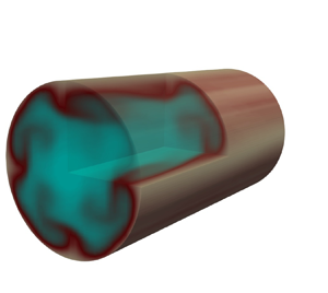
We turn our attention to an RPO with period  $T=26.64$ in pipe flow, whose ECS have been found to closely resemble the near-wall quasistreamwise vortices that characterise wall turbulence (Willis, Cvitanović & Avila Reference Willis, Cvitanović and Avila2013). Pipe flow exhibits inherent periodicity in the azimuthal direction and maintains a consistent mean streamwise velocity. Here, the fixed-flux Reynolds number is $Re=DU/\nu =2500$, where length and velocity scales are non-dimensionless by the diameter (D) and velocity (U), respectively. We consider the minimal flow unit in the $m=4$ rotational space (‘shift-and-reflect’ invariant space); thus, the computational domain $\varOmega =[1/2,2{\rm \pi} /m,{\rm \pi} /\alpha ]\equiv {(r,\theta,z)\in [0,1/2]\times [0,2{\rm \pi} /m]\times [0,{\rm \pi} /\alpha ]}$, where $L={\rm \pi} /\alpha$ stands for the length of the pipe and $\alpha =1.7$ (as in previous work from Willis et al. Reference Willis, Cvitanović and Avila2013; Budanur et al. Reference Budanur, Short, Farazmand, Willis and Cvitanović2017). In wall units, this domain is $\varOmega ^+ \approx [100,160,370]$, which compares well with the minimal flow units for Couette flow and channel flow.
Data was generated with the pseudospectral code Openpipeflow with  $\Delta t=0.01$ on a grid $(N_r,M_\theta,K)=(64,12,18)$, then, following the $3/2$ rule, variables are evaluated on $64\times 36\times 54$ grid points; thus, $u\in \mathbb {R}^{124,416}$ (Willis Reference Willis2017) (where $N_r$, $M_\theta$ and $K$ correspond to the non-uniform spaced points in the radius, and the total Fourier modes in $\theta$ and z, respectively). We ran simulations forward on time, and stored $10^3$ time units at intervals of $0.1$ time units. Pipe flow is characterised by the presence of continuous symmetries, including translation in the streamwise direction and azimuthal rotation about the pipe axis. We phase-align the data for both continuous symmetries using the first Fourier mode method of slices to improve the effectiveness of the dimension reduction process (Budanur, Borrero-Echeverry & Cvitanović Reference Budanur, Borrero-Echeverry and Cvitanović2015).
To find the manifold dimension and its coordinates, we first perform a linear dimension reduction from  $O(10^5)$ to $O(10^2)$ with POD. Figure 4(a) displays the eigenvalues, $\mu _i$, of POD modes sorted in descending order. We select the leading 256 modes that capture the $99.99\,\%$ of the total energy of the system. Most of these modes are characterised by being complex (i.e. two degrees of freedom), so projecting onto these modes results in a 508-dimensional POD coefficient. Next, we perform nonlinear dimension reduction in the POD coordinates using IRMAE-WD. Figure 4(b) shows the singular values $\sigma _i$ resulting from performing SVD on the covariance matrix of the latent data matrix from the autoencoder. The singular values for $i>2$ drop to ${\approx }10^{-6}$, indicating that the dimension of the manifold is $d_\mathcal {M}=2$ which is the correct embedding dimension for an RPO, given that we have factored out the continuous symmetries as noted above. We reiterate that we have elucidated the precise embedding dimension of the manifold, commencing from an initial state dimension of $O(10^{5})$.
Pipe flow with  $Re=2500$: periodic orbit regime. (a) Eigenvalues of POD modes sorted in descending order. (b) Identification of $\mathcal {M}$: normalised singular values of the latent space data with a drop at $d_\mathcal {M}=2$. (c) Eigenvalues of the Koopman operator (the right panel shows a magnified view of the eigenvalues). (d) Comparison of the norms of the velocity field between the models and the true data. (e) Reynolds stresses varying with the radial position from the ground truth, Koopman and NODE predictions; the labels are on the plot. (f) Two-dimensional representation of the dynamics in a $z\unicode{x2013}\theta$ plane $(r = 0.496)$ with $u_z$ for the true and predicted dynamics at $t=200$.

Having found the mapping to  $\mathcal {M}$, we apply both the function and state approaches on $\mathcal {M}$, and evolve the same initial condition forward on time out to 200 time units (e.g. 7.5 periods). Figure 4(c) shows the eigenvalues of the Koopman operator (with $100$ dictionary elements), and, identically to the previous cases, some of them have unit magnitude $|\lambda _k|=1$; thus, the long-time dynamics will not decay. Figure 4(d) displays time evolution of the norm of the velocity field in which the NODE and Koopman predictions can capture the true dynamics (here the norm is defined to be the $L_2$ norm $\| {\boldsymbol {u}} \|_2^2=(1/V)\int {\boldsymbol {u}}\boldsymbol{\cdot}{\boldsymbol {u}}\, {\rm d}{\boldsymbol {r}}$), where V is the volume of the domain. To further demonstrate that the evolution of the dynamics on $d_\mathcal {M}$ is sufficient to represent the state in this case, we examine the reconstruction of statistics. In figure 4(e), we show the reconstruction of four components of the Reynolds stress $\langle u_z^2 \rangle, \langle u_\theta ^2 \rangle, \langle u_r u_z \rangle$ and $\langle u_r^2 \rangle$ (the remaining two components are relatively small). The Reynolds stresses evolved on $d_\mathcal {M}$ closely match the ground truth. Lastly, figure 4(f) displays field snapshots in the $z\unicode{x2013}\theta$ plane ( $r=0.496$) at $t=200$, respectively showing qualitatively that the models can capture perfectly the dynamics of the true system.
4. Conclusion
In this study, we have presented a framework that leverages data-driven approximation of the Koopman operator, and NODE to construct minimal-dimensional models for exact coherent states to the NSE within manifold coordinates. Our approach integrates an advanced autoencoder-based method to discern the manifold dimension and coordinates describing the dynamics. Subsequently, we learn the dynamics using both function-space-based and state-space-based approaches within the invariant manifold coordinates. We have successfully applied this framework to construct models for exact coherent states found in Kolmogorov flow and minimal flow unit pipe flow. In these situations, performing fully resolved simulations would necessitate a vast number of degrees of freedom. However, through our methodology, we have effectively reduced the system's complexity from approximately  $O(10^5)$ degrees of freedom to a concise representation comprising fewer than three dimensions, which is capable of faithfully capturing the dynamics of the flow such as the Reynolds stresses for pipe flow, and the average rate of dissipation and power input for Kolmogorov flow. These results illustrate the capability of nonlinear dimension reduction with autoencoders to identify dimensions and coordinates for invariant manifolds from data in complex flows as well as the capabilities of both state-space and function-space methods for accurately predicting time evolution of the dynamics on these manifolds.
By accurately modelling coherent state dynamics with far fewer degrees of freedom than required for direct numerical simulation, manifold dynamics models like those reported here open the possibility for dynamical-systems-type analyses such as calculation of Floquet multipliers or local Lyapunov exponents in a computationally highly efficient way. These models also facilitate the application of control strategies with minimal degrees of freedom. An illustrative example is the application of reinforcement learning techniques in controlling planar minimal flow unit (MFU) Couette flow (see Linot, Zeng & Graham Reference Linot, Zeng and Graham2023b). The linear representation of the dynamics via the Koopman operator facilitates control using well-established techniques, such as the linear quadratic regulator (LQR), resulting in efficacious optimal control for nonlinear systems (Otto & Rowley Reference Otto and Rowley2021).
Finally, we have also successfully showcased the efficacy of both the function and the state-space approaches in handling coherent state dynamics. When implementing the function-space approach, we underscored the critical significance of dimension reduction for the construction of the observable space. When applying EDMD-DL on the full-state data for pipe flow, the computational challenges escalate significantly when attempting to handle an observable space dimensionality exceeding  $O(10^5)$. Therefore, dimension reduction techniques are pivotal in making both the function and the state-space approaches feasible and computationally efficient, ensuring practical applicability to real-world scenarios.
Acknowledgements
We wish to thank Dr Ashley. P. Willis for making the ‘openpipeflow’ code open source, and his help to setup the simulations.
Funding
This work was supported by ONR N00014-18-1-2865 (Vannevar Bush Faculty Fellowship).
Declaration of interests
The authors report no conflict of interest.


 Open access

