3.1. Flow visualisations

This section explores the evolution of the near-wall turbulent structures during the pulsation cycle for three cases (L26A05, L26A10 and L10A10), to provide an overview of the flow behaviour and turbulent mechanisms in play. The turbulent vortical structures are visualised through isosurfaces of $\lambda _2$, which denote the second eigenvalue of the symmetric component of the velocity gradient tensor. The near-wall velocity streaks are visualised through positive and negative values of the streamwise fluctuating velocity component, $u^\prime =u-\langle u\rangle$. The mean velocity reference value of $\langle u\rangle$ is taken from the phase-averaged value at the corresponding wall-normal location at each point. Each visualisation comprises of eight flow fields which are evenly spaced by a phase interval of $0.25{\rm \pi}$. Two additional flow fields are included at $\phi =0.875{\rm \pi}$ and $\phi =1.125{\rm \pi}$, in order to provide greater clarity to the transitional behaviour of case L26A10.

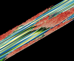
At the start of the acceleration period in case L26A05 (figure 5), the near-wall flow is still undergoing a process of turbulence decay, which was initiated during the preceding deceleration phase. As the flow accelerates, the remaining vortical structures continue to gradually degrade, whilst the streamwise velocity fluctuations are further suppressed. At $\phi =0.25{\rm \pi}$, the rate of decay in the vortical structures has slowed substantially, leaving the remaining vortical structures, which remain loosely dispersed over the surface, to convect downstream. At the same time, the remaining weak streamwise velocity streaks begin to grow and elongate. As the flow passes the midpoint of the acceleration period, new vortical structures begin to form in clusters that are mostly concentrated around the low-speed velocity streaks. The clusters of vortical structures, which indicate the presence of highly concentrated turbulent spots, continue to grow in size until they begin to merge. The evolution of the vortical structures between $\phi =0.25{\rm \pi}$ and $\phi =0.875{\rm \pi}$ closely resembles the pretransition stage of non-periodic acceleration (He & Seddighi Reference He and Seddighi2015). By comparing figure 5 to the ramp-up flow case of Seddighi et al. (Reference Seddighi, He, Vardy and Orlandi2014) these similarities become even more striking. During the remainder of the acceleration period and the early deceleration period there is no significant change in the density or distribution of the vortical structures at the wall. However, by $\phi =1.5{\rm \pi}$ the density of the vortical structures is visibly reduced as turbulence begins to decay towards the weakly turbulent flow field seen at $\phi =0$.

Figure 5. Development of the streamwise velocity streaks and turbulent vortices for case L26A05: $\lambda _2/(\overline {U_b}/\delta )^2=-5$ (red); $u^\prime /\overline {U_b}=-0.2$ (blue); $u^\prime /\overline {U_b}=0.2$ (green).

As for case L26A05, the flow field at the start of acceleration in case L26A10 (figure 6) is still in a stage of turbulence decay. However, in case L26A10 the vortical structures continue to diminish until $\phi =0.25{\rm \pi}$, when the flow in the near-wall region comes close to resembling a fully laminar state. The flow does not immediately enter a stage of velocity streak growth, and there is a delay in the formation of low- and high-speed velocity streaks. The flow remains frozen in a weakly turbulent (almost laminar-like) state until the first streamwise velocity streaks begin to form anew at $\phi =0.375{\rm \pi}$. The flow then follows the same pattern seen in figure 5 and Seddighi et al. (Reference Seddighi, He, Vardy and Orlandi2014), and thus begins a process of bypass-like transition. However, there are key differences in the evolution of the flow in figure 6 when compared with the lower amplitude case in figure 5. Firstly, and most notably, there is a delay in the formation of the turbulent spots around the low-speed streaks. These spots do not begin to form until $\phi =0.75{\rm \pi}$, at which time the turbulent spots in case L26A05 were already beginning to merge. Due to this delay, there is insufficient time for the bypass-like transition process to complete, and the flow reaches the start of the deceleration period before the turbulent spots have started to merge. Secondly, the turbulent spots in case L26A10 are much more refined, and consist of a greater number of vortical structures which are packed together with greater density. Finally, the streamwise velocity streaks in case L26A10 undergo far greater elongation, with a maximum length that is approximately three times larger than that seen in case L26A05. Seddighi et al. (Reference Seddighi, He, Vardy and Orlandi2014) identified such differences in the growth of turbulent spots and velocity streaks when comparing ramp-up and step-up acceleration in non-periodic accelerating flows at an equivalent Reynolds number. During the acceleration, an amplitude of $A_b=0.5$ (case L26A05) more closely mimics a ramp-up flow acceleration, whilst an amplitude of $A_b=1.0$ (case L26A10) more closely mimics a step-up acceleration. As in the ramp-up acceleration of Seddighi et al. (Reference Seddighi, He, Vardy and Orlandi2014), for an amplitude of $A_b=0.5$ the flow completes transition before the maximum bulk velocity is reached, whilst this is not true for the higher amplitude of $A_b=1.0$.

Figure 6. Development of the streamwise velocity streaks and turbulent vortices for case L26A10: $\lambda _2/(\overline {U_b}/\delta )^2=-5$ (red); $u^\prime /\overline {U_b}=-0.2$ (blue); $u^\prime /\overline {U_b}=0.2$ (green).

Figure 6 shows that the flow in case L26A10 begins the deceleration period in the early stages of bypass-like transition. At this point, the developing turbulent spots are limited to a few discrete locations and vortical structures are absent over the majority of the surface. It is natural to expect that such an incomplete transition process will fail to reach a fully turbulent state under a continuously increasing deceleration rate. However, during the initial deceleration period the turbulent spots continue to grow and start to merge. By $\phi =1.25{\rm \pi}$ the vortical structures cover the majority of the surface. Throughout the second half of the deceleration period, these vortical structures diminish along with the streamwise velocity streaks, as the turbulence decays towards the weakly turbulent state at $\phi =0$. The persistence of the transition process can be explained by considering the response of an equivalent non-periodic flow. When a fully developed turbulent flow is subject to a ramp-down deceleration, there is a delay in the response of the turbulence in the early stages of deceleration (Guerrero et al. Reference Guerrero, Lambert and Chin2023). During this delay, the Reynolds shear stress only undergoes a very gradual change in the near-wall region, such that turbulence remains effectively frozen in its initial state. This delayed turbulence response can also be confirmed for case L26A05, as can be seen in figure 5, and as will be further discussed in more detail in § 3.3. These findings suggest that the concept of a frozen turbulence response can be expanded in the context of pulsating flow to include both the existing turbulence structures, and the temporally evolving mechanism of bypass-like transition.

The similarity between free-stream turbulence induced bypass transition and the behaviour observed in figures 5 and 6 can be confirmed through the assessment of turbulent kinetic energy variations during streak development. Figure 7 displays the evolution of the wall-normal maximum values of the turbulent kinetic energy and its three velocity components; $\langle u^\prime u^\prime \rangle ^+_{max}$, $\langle v^\prime v^\prime \rangle ^+_{max}$ and $\langle w^\prime w^\prime \rangle ^+_{max}$, throughout the cycle. In the early stages of free-stream turbulence bypass transition, the elongation of the streaks is reflected in the linear growth of $\langle u^\prime u^\prime \rangle ^+_{max}$ and turbulent kinetic energy ($2\langle TKE\rangle ^+_{max}$) with streamwise distance (Matsubara & Alfredsson Reference Matsubara and Alfredsson2001; Fransson, Matsubara & Alfredsson Reference Fransson, Matsubara and Alfredsson2005), or time in the case of the pretransition stage of temporal acceleration (He & Seddighi Reference He and Seddighi2013). Furthermore, since this early growth of $\langle u^\prime u^\prime \rangle ^+_{max}$ is not caused by amplified turbulence generation, the maximum wall-normal and spanwise velocity motions should be relatively unaffected prior to the destabilisation of the streaks. From figures 5 and 6 it is clear that in cases L26A05 and L26A10 the initial growth of turbulent energy is attributed almost entirely to the amplification of the streamwise turbulent motions, whilst the gradual decay of $\langle v^\prime v^\prime \rangle ^+_{max}$ and $\langle w^\prime w^\prime \rangle ^+_{max}$ adversely impacts the turbulent energy growth. Hence, it can be concluded that the growth of $\langle u^\prime u^\prime \rangle ^+_{max}$ is an artificial amplification which is attributed primarily to streak elongation, as characteristic of bypass transition. In figure 7(c,d) similar behaviour is observed for cases L16A05 and L16A10, such that together, these four cases represent the four instances of a bypass-like transition observed in the present study. Reducing the Stokes length further (as shown in figure 7e) extends the artificial growth of turbulent kinetic energy far into the deceleration period. The flow then deviates from bypass-like transition behaviour, since the decay of $\langle u^\prime u^\prime \rangle ^+_{max}$ counteracts the natural growth of $\langle v^\prime v^\prime \rangle ^+_{max}$ and $\langle w^\prime w^\prime \rangle ^+_{max}$ as the streaks destabilise.

Figure 7. Phase-variance of the maximum Reynolds stress components and turbulent kinetic energy for cases (a) L26A05, (b) L26A10, (c) L16A05, (d) L16A10 and (e) L10A10. Arrows indicate the respective axis for the intersecting curves. Vertical blue lines indicate the initiation of turbulence growth/transition. The appropriate location of each line was determined from the analysis in § 3.3.

When the Stokes length is reduced to $l_s^+=10$, for an amplitude of $A_b=1.0$ (case L10A10, figure 8), the flow undergoes the early stages of bypass-like transition, but fails to reach a fully turbulent state before the end of the deceleration period. Therefore, the critical limit for which a current-dominated flow can undergo a full turbulent–turbulent transition process can be assumed to lie within the range of $l_s^+=10$ to $l_s^+=16$. At the start of the acceleration period, turbulence remains strong at the wall, with vortical structures covering the surface, though with a greater density around the elongated low-speed velocity streaks. At this point, the vortical structures and velocity streaks are convecting in the reverse direction, due to a reversal of the flow at the wall during the late deceleration period. As the flow accelerates, the turbulence starts to decay and the vortical structures are diminished, whilst the streamwise velocity streaks break up. New streamwise velocity streaks begin to form towards the end of the acceleration period, though by $\phi ={\rm \pi}$ there is no sign of turbulent spots, and a significant amount of ‘old’ turbulence still lingers in the flow. At $\phi =1.5{\rm \pi}$ a clustering of new vortical structures can be observed around the low-speed velocity streaks, indicating the growth of turbulent spots consistent with bypass transition. Throughout the second half of the deceleration period these clusters grow very slowly. This growth continues even as the near-wall flow is reversed, and the early stages of merging can be observed. However, this is as far as the process gets, and growth of turbulent spots is heavily suppressed throughout the remainder of the deceleration period.

Figure 8. Development of the streamwise velocity streaks and turbulent vortices for case L10A10: $\lambda _2/(\overline {U_b}/\delta )^2=-5$ (red); $u^\prime /\overline {U_b}=-0.2$ (blue); $u^\prime /\overline {U_b}=0.2$ (green).

3.2. Streamwise velocity streaks

The properties of the near-wall velocity streaks can be quantified through a two-point correlation of the streamwise velocity field (3.1a,b). The streamwise correlation $R_{11x}$ quantifies the length of the streaks, whilst the spanwise correlation $R_{11z}$ quantifies the spanwise spacing between the streaks, which is assumed to be equal to twice the spanwise distance at which $R_{11z}$ reaches its minimum value, $(R_{z11})_{min}$. The magnitude of $(R_{z11})_{min}$ indicates the strength of the streaks relative to the surrounding flow in the corresponding $x$–$z$ plane (Mathur et al. Reference Mathur, Seddighi and He2018b; Falcone & He Reference Falcone and He2022),

(3.1a,b)\begin{align} R_{iix}(\kern0.7pt y,x_1) = \frac{\langle u^\prime_i(x,y,z)u^\prime_i(x+x_1,y,z)\rangle}{\langle u_i^{\prime2}(x,y,z)\rangle},\quad R_{iiz}(\kern0.7pt y,z_1) = \frac{\langle u^\prime_i(x,y,z)u^\prime_i(x,y,z+z_1)\rangle}{\langle u_i^{\prime2}(x,y,z)\rangle}. \end{align}

Case L26A05 starts the acceleration period with weak streaks with no clearly defined or uniform spacing. However, figure 9(a) confirms that that by $\phi =0.625{\rm \pi}$, strong velocity streaks have formed, with a consistent spacing of $2z^+=160$. As the streaks are stretched, they maintain this spacing, whilst growing in strength. Following their destabilisation and resultant breakup, the strength of the streaks degrades, and their spacing shrinks, before plateauing around $2z^+=80$. This strength and spacing remains effectively frozen during early deceleration. After $\phi =1.25{\rm \pi}$ the streaks begin to decay and lose their form, until a clear minimum of $R_{z11}$ is no longer visible, though they never fully dissipate.

Figure 9. Distribution of the two-point correlation of spanwise velocity for cases (a) L26A05, (b) L26A10 and (c) L10A10.

During the initial acceleration period in case L26A10 (figure 9b), $R_{11z}$ remains positive for all spacings of $2z^+<400$ throughout the domain. The velocity streaks that emerged during the preceding turbulent–turbulent transition process have almost completely decayed, and by $\phi =0$ their remaining decay has a minimal impact on the weak turbulence field. At $\phi =0.375{\rm \pi}$, new velocity streaks are beginning to take shape, which converge to a clearly defined spacing of $2z^+\approx 160$ by $\phi =0.5{\rm \pi}$ (figure 9b). This approximate spacing is maintained throughout the remaining life cycle of the streaks, right up until their disintegration. The streaks elongate and grow in strength throughout the remainder of the acceleration period, even after $\phi =0.75{\rm \pi}$, when the magnitude of the minimum value of $R_{11z}$ falls as the streaks begin to destabilise. The strength of the streaks prior to transition is significantly greater than that in case L26A05. However, at $\phi =1.25{\rm \pi}$, $R_{z11}$ has once again become positive for $2z^+<400$ throughout the domain, indicating a complete breakdown of the streaks by this point. This behaviour in $R_{11z}$ bears a strong similarity to that observed in the step-up accelerating flows of Mathur et al. (Reference Mathur, Seddighi and He2018b), in which the Reynolds number was increased by a large factor of 6.5. When this factor was raised to 19.3, for the same initial Reynolds number, the positive values of $R_{11z}$ at the point of transition further increased in value, and the positive region spanned a significantly greater spanwise spacing. Compare this to the weaker step-up of acceleration of He & Seddighi (Reference He and Seddighi2013), which started with the same initial Reynolds number as Mathur et al. (Reference Mathur, Seddighi and He2018b), but only increased the Reynolds number by a factor of 2.62. Around the point of transition, the profiles of $R_{11z}$ rapidly fell towards the zero axis with increasing spanwise distance, only deviating from this trend for negative values of $R_{11z}$. The present results suggest that, at an amplitude of $A_b=1.0$, the Stokes length of a pulsating flow may exert a similar influence on the distribution of $R_{11z}$ around the point of transition, as that exerted by the Reynolds number ratio during step-up acceleration.

Case L10A10 (figure 9c) starts off in a similar manner to case L26A05. During acceleration, the existing streaks become much weaker as the existing turbulence continues to decay following the preceding cycle. At $\phi =0.875{\rm \pi}$ a clearly defined spacing can be observed, as new streaks begin to develop. By the end of the acceleration period the spacing between the streaks has shrunk to $2 z^+\approx 100$, and the strength of the streaks has increased substantially. Throughout the first half of the deceleration period there is minimal change in both the spacing and the strength of the streaks (figure 9c). However, small sinuosities start to form in the low-speed streaks. Such sinusoidal deformations have been identified as the initial instability from which streak breakdown typically occurs in bypass transition (Schlatter et al. Reference Schlatter, Brandt, de Lange and Henningson2008). The development of the sinuosities is slow, relative to the phase of the cycle, such that the elongated velocity streaks remain mostly intact by $\phi =1.5{\rm \pi}$. In terms of inner-scaled time, these sinuosities grow at comparable rates between different strokes lengths for $A_b=1.0$. Sinuosity development for $l_s^+=10$ spans a period of $\Delta t^+=78$. Consider that the snapshots of case L26A10 in figure 10 are spaced by $\Delta t^+=130.8$ apart. After the appearance of the first sinuosity, it takes $\Delta t^+=130.8$ for the instability to develop into a local breakdown of the streak, and at least an additional $\Delta t^+=130.8$ for the turbulent spot to grow sufficiently to begin merging. Additional time will be required before new turbulence growth will propagate into the core $(\kern0.7pt y^+=106.4)$, where the turbulence field has shown only minor changes between $\phi =0.75{\rm \pi}$ and $\phi ={\rm \pi}$. By comparison, time between the first sinuosity and the first turbulent spot in a flow of $l_s^+=16$ is $\Delta t^+=100$, with a further $\Delta t^+=75.0$ for merging to occur. Although these processes occur at different phases in the cycle, and hence, at different bulk velocities, the growth rate of the sinous instabilities appears to be unaffected by the local bulk velocity, at least in the late acceleration period and early deceleration period.

Figure 10. Growth of a secondary sinuous instability of the streamwise velocity streaks at $y^+=12.4$, and its propagation at $y^+=106.4$, for case L26A10.

3.3. Turbulent statistics

During turbulent–turbulent transition in non-periodic acceleration, the temporal evolution of the Reynolds stress components follow a multistage process which correlates to the changes of near-wall turbulent structures (He & Seddighi Reference He and Seddighi2015). These stresses are important in accurately defining both the temporal limits and characteristic behaviours of the distinct stages of the turbulent–turbulent transition process. To understand the flow of energy between the components, we also assess the temporal evolution of the terms in the turbulent energy budget for the streamwise Reynolds stress component (3.2); the production $P_{11}$, viscous dissipation $e_{11}$, pressure strain $\varPi _{11}$, pressure diffusion $\varGamma _{11}$, turbulent transport $T_{11}$ and viscous diffusion $D_{11}$. The wall-normal and spanwise components do not gain energy directly from newly generated turbulence. Their primary source comes from the transfer of energy from the streamwise component, which is governed by the pressure strain. Hence, $P_{11}$, which acts at the primary source of newly generated turbulent energy, and $\varPi _{11}$, serve as the most critical budget terms which govern the turbulence response to unsteady forcing,

(3.2) \begin{equation} \left. \begin{array}{@{}ll} P_{11}={-}2\langle u^\prime v^\prime \rangle \left\langle\dfrac{\partial u}{\partial y}\right\rangle, & {e_{11}={-}2\nu\left\langle\dfrac{\partial u^\prime }{\partial y}\dfrac{\partial u^\prime }{\partial y}\right\rangle,}\\ \varPi_{11}=2\left\langle p^\prime \dfrac{\partial u^\prime}{\partial x}\right\rangle, & {\varGamma_{11}={-}2\dfrac{\partial \langle p^\prime u^\prime\rangle}{\partial x},}\\ {T_{11}={-}\dfrac{\partial \langle u^\prime v^\prime w^\prime\rangle}{\partial y},} & {D_{11}=\nu\dfrac{\partial^2 \langle u^\prime u^\prime \rangle}{\partial^2 y}.} \end{array} \right\} \end{equation}

The phase-variance of the production, pressure strain, viscous dissipation, turbulent transport and viscous diffusion streamwise budget terms are displayed alongside the Reynolds stress components for cases L26A05 (figure 11), L26A10 (figure 12) and L16A10 (figure 13). The pressure-diffusion term $\varGamma _{11}$ is negligible for the streamwise component, and hence, is excluded from this analysis. The evolution of Reynolds stress components and streamwise budgets terms (3.2) in case L16A05 closely resembles that of case L16A10, and so the corresponding plots for the former case have been excluded for clarity. For these pulsating flows, we have decomposed the turbulent–turbulent transition cycle in five distinct stages: the (I) residual decay; (II) pretransition; (III) transition; (IV) post-transition; (V) turbulence decay stages.

Figure 11. Phase-variance of the Reynolds stress components and streamwise energy budget terms for case L26A05.

Figure 12. Phase-variance of the Reynolds stress components and streamwise energy budget terms for case L26A10.

Figure 13. Phase-variance of the Reynolds stress components and streamwise energy budget terms for case L16A10.

In case L26A05 (figure 11), immediately following acceleration there is a short delay before the elongation of velocity streaks which signals the beginning of a pretransition stage. During this delay, $v^\prime _{rms}$ and $-\langle u^\prime v^\prime \rangle$ show minimal change at $y^+=12.0$ and $y^+=5.4$, whilst they gradually decay farther away from the wall. Meanwhile $w^\prime _{rms}$ shows a continuous decay throughout the domain. These same trends are also observed in varying degrees for other intermediate and low-frequency cases (figures 12 and 13). At first glance, it is tempting to attribute this behaviour of decay to the growth of a new laminar boundary layer, and the displacement of existing turbulent structures away from the wall. However, this cannot be the case, since in non-periodic accelerating flows the perturbation flow field remains independent of the base flow, and exerts no significant change in $v^\prime _{rms}$ and $w^\prime _{rms}$, prior to the onset of transition (Seddighi et al. Reference Seddighi, He, Vardy and Orlandi2014; He & Seddighi Reference He and Seddighi2015; Guerrero et al. Reference Guerrero, Lambert and Chin2021). Instead, this response represents a continuation of ongoing turbulence decay which started within the preceding deceleration period, as will be further discussed later in this section. We refer to the period of this delay as the ‘residual decay’ stage, which is unique to periodic acceleration in pulsating flows.

The pretransition stage is marked by a gradual growth of $u^\prime _{rms}$. As in the case of non-periodic accelerating flow, the growth of $u^\prime _{rms}$ stems primarily from the elongation of high- and low-speed streamwise velocity streaks and not from the generation of new turbulence. However, this elongation does produce a mild response in the streamwise production term $P_{11}$. This occurs because the streamwise production term depends on the Reynolds shear stress, see (3.2), which in turn relies on the strength of both the streamwise and wall-normal turbulent motions. Since $v^\prime _{rms}$ remains effectively frozen during pretransition, the streak elongation causes production to grow gradually in line with $u^\prime _{rms}$. Case L26A10 (figure 12) presents an exception to this behaviour, as the near-total decay of $v^\prime _{rms}$ close to the wall ensures that the Reynolds shear stress, and hence streamwise production, remains suppressed despite the growth of $u^\prime _{rms}$. In contrast to non-periodic acceleration, the wall-normal and spanwise Reynolds stresses do not remain frozen during pretransition. Whilst $v^\prime _{rms}$ shows minimal change at the wall, its strength continues to diminish within the core, $w^\prime _{rms}$ falls continuously throughout the domain. Clearly, the ongoing process of turbulence decay, and its propagation into the core, from preceding stages (I and V), remains active. Since the pressure strain is heavily suppressed prior to destabilisation, this decay process initially constitutes the primary mechanism governing the evolution of $v^\prime _{rms}$ and $w^\prime _{rms}$.

In the present study, the transition stage is the most sharply defined out of all stages in the periodic turbulent–turbulent transition process. Its beginning is marked by the rapid shift in the growth rate in the streamwise production term. This is followed by a rapid growth of $\varPi _{11}$, which indicates that the critical turbulent mechanism of redistributing energy to the wall-normal and transverse motions becomes highly active. The elongation of velocity streaks is no longer the primary mechanism for extracting turbulent energy from the flow, and the evolution of $P_{11}$ now represents the amplification of true turbulent energy production. Comparison between figures 5 and 6 makes it clear that this new energy originates from destabilisation and breakup of low-speed velocity streaks, and the growth of highly concentrated turbulent spots. In all cases, this process causes a ‘violent explosion’ of the Reynolds stresses at the wall, at least in the case of $v^\prime _{rms}$, $w^\prime _{rms}$ and $-\langle u^\prime v^\prime \rangle$. So far, this behaviour closely mimics the turbulent–turbulent bypass transition of a perturbation boundary layer for non-periodic acceleration (He & Seddighi Reference He and Seddighi2013). In each case, the transition stage is marked by an accelerated growth rate in $u^\prime _{rms}$, spurred on by the enhanced production of new turbulent energy. However, at the end of transition, case L26A05 (figure 5) is the only case to display an overshoot of $u^\prime _{rms}$ in the buffer layer, as is characteristic of the transition in non-periodic acceleration (Jung & Kim Reference Jung and Kim2017). The reason for this relates to the deceleration period and will be elaborated on further in the discussion of stage V.

In non-periodic acceleration, completion of transition is followed by a final stage of relaxation, in which near-wall turbulence settles into a state of equilibrium, whilst the core region waits to settle through the slow process of turbulent propagation from the wall. In all cases where the transition stage extends into the deceleration period (figure 12 and 13) there is insufficient time for such relaxation, as the growing deceleration rate quickly ensures that turbulence decay takes over as the main transient turbulence process. However, in case L26A05, figure 11 shows that if the transition stage ends whilst the flow is still accelerating, then an intermediate stage emerges. By $\phi =0.875{\rm \pi}$ the growth rates of $P_{11}$ and $\varPi _{11}$ are beginning to slow down. As a result, the growth rates of all Reynolds stress components in the near-wall region fall substantially, particularly in the case of $u^\prime _{rms}$, $v^\prime _{rms}$ and $w^\prime _{rms}$. These three components then settle onto a relatively flat peak around their maximums. Meanwhile the strength of Reynolds stress components away from the wall ($\kern0.7pt y^+=106.4$) continues to grow, as new turbulence at the wall continues to propagate into the core. Whilst this stage shares many characteristics with the ‘core relaxation’ stage of non-periodic acceleration (Guerrero et al. Reference Guerrero, Lambert and Chin2021), its lifespan is only a fraction of the time scales needed for propagation of enough turbulence to bring the core into equilibrium. By $\phi =1.25{\rm \pi}$, the Reynolds stress components close to the wall have already begun to decay whilst those at $y^+=106.4$ are continuing to grow. Furthermore, at $y^+=5.4$ and $y^+=12.4$ the production and viscous dissipation (figure 11e,g), which reached their peak at the end of the transition stage, are becoming gradually weaker throughout the latter half of stage IV. With these differences in mind, this stage of the pulsating cycle could be reclassified in more general terms as a ‘post-transition’ stage, in which non-periodic and periodic acceleration share a common characteristic of a continuous growth of Reynolds stress components in the core, and a partially shared characteristic regarding the reduced growth rate of these stresses in the near-wall region. Their only variation lies in the severity of growth rate reduction, which does not completely reduce to zero in periodic acceleration.

Over a majority of the deceleration period all Reynolds stress components show a continuous reduction in strength which slows down as the flow approaches its initial state at $\phi =2{\rm \pi} (0)$. In each case, the process begins at the wall, first with $u^\prime _{rms}$, and then, after a short delay, continuing with $v^\prime _{rms}$ and $w^\prime _{rms}$, which occurs simultaneously. Each response is precipitated by the reduction of its respective primary source term ($P_{11}$ and ${\varPi }_{11}$). Once again, there is a delayed response in the core, as turbulence generated during the preceding transition or post-transition stage is initially still propagating towards the core region. For case L26A05, turbulent shear stress begins to decay at $\phi ={\rm \pi}$, whilst for the remaining three cases its decay occurs simultaneously with that of $v^\prime _{rms}$ and $w^\prime _{rms}$. During the pretransition stage $u^\prime _{rms}$ and $-\langle u^\prime v^\prime \rangle$ were shown to not be reliable indicators of true turbulence generation. With this in mind, we opt to define a starting point for the turbulence decay stage as the point at which $v^\prime _{rms}$ and $w^\prime _{rms}$ begin to decay.

It is important to note that, in the absence of a distinct post-transition stage (figures 12 and 13), any potential overshoot in $u^\prime _{rms}$ towards the end of transition is masked by the sudden dominance of the decay process in the turbulence decay stage. By comparison, this overshoot is clearly visible in figure 11, such that $u^\prime _{rms}$ peaks at the wall, before briefly settling towards a pseudoequilibrium value. This distinction is important to keep in mind, as the overshoot of $u^\prime _{rms}$ is a typical feature of turbulent–turbulent transition, and has been offered as a reliable criterion for its detection in non-periodic acceleration (Jung & Kim Reference Jung and Kim2017). The present results confirm that this criterion can be valid for certain pulsating flows, but should be applied selectively based upon the phase within which the transition stage concludes.

3.4. Perturbation flow field

The turbulent–turbulent transient process is initiated by the growth and destabilisation of a temporally developing perturbation boundary layer at the wall. He & Seddighi (Reference He and Seddighi2015) showed that the perturbation boundary layer can be obtained from a decomposition of an unsteady flow into two flow fields: a perturbation flow and a base flow. The base flow is time-independent, and is usually taken as either the initial flow field in the case of non-periodic flow, or the time-averaged flow field in the case of periodic flow. The perturbation flow is time-dependant and represents the difference between the flow field at a point in time and the base flow. In practical terms, the perturbation flow represents the change in the flow field which results from the unsteady forcing. Although the present investigation concerns a pulsating flow, the perturbation flow is defined as though the flow was a non-periodic accelerating flow. The base flow is taken as the flow field at the point of minimum bulk velocity $(\phi =0)$ for both the acceleration and deceleration periods of the pulsation cycle. The perturbation velocity for the present case is given as

(3.3)\begin{equation} u^\wedge(\kern0.7pt y,t)=\frac{\langle u\rangle(\kern0.7pt y,t)-\langle u\rangle(\kern0.7pt y,0)}{\langle u\rangle(\delta,t)-\langle u\rangle(\delta,0)}\rightarrow\frac{\langle u\rangle(\kern0.7pt y,t)-\langle u\rangle(\kern0.7pt y,0)}{A_{uc}\left(1-\cos(\omega t)\right)}. \end{equation}

Two theoretical laminar flow scenarios are considered: Stokes first problem for a flow accelerating from rest; and Stokes second problem for an oscillating flow. At first glance, the former scenario may be assumed to be irrelevant in the context of pulsating flows. However, as shown, Stokes first problem provides a close representation of laminar perturbation development during the pretransition stage of certain low-frequency, pulsating flows. The solution to Stokes second problem for a laminar flow in a channel is given as

(3.4)\begin{equation} u_{osc}=A_{uc}{\rm Re}\left[{\rm i}\left(\frac{\cosh\left(\kern0.7pt y\sqrt{{\rm i}\omega/\nu}\right)}{\cosh\left(\delta\sqrt{{\rm i}\omega/\nu}\right)}-1\right){\rm e}^{{\rm i}\omega t}\right]. \end{equation}

For an accelerating or decelerating flow with an arbitrary, time-varying acceleration rate, the solution to Stokes first problem is given by the extended Stokes solution, (Schlichting & Gersten Reference Schlichting and Gersten2017)

(3.5)\begin{equation} u_{ext}(\kern0.7pt y,t)=\int_{0}^{t}\frac{{\rm d}U_b(\xi)}{{\rm d}\xi}\, {\rm erf}\left(\frac{y}{2\sqrt{\nu (t-\xi)}}\right)\,{\rm d}\xi, \end{equation}

where ‘erf’ represents the error function of the form $\textrm {erf}(\psi )=({2}/{\sqrt {{\rm \pi} }})\int ^{\psi }_{0}\textrm {e}^{-\gamma ^2}\,\textrm {d}\gamma$.

The $\cosh$ function in (3.4) can be solved through a series expansion, although the expansion is slow to converge for all but very low frequencies ($\omega \rightarrow 0$). For very high frequencies ($\omega \rightarrow \infty$) the $\cosh$ function can be expressed in the asymptotic formula $\cosh (\psi )\rightarrow 0$. This simplification produces the quasilaminar solution for Stokes second problem which is valid in the high-frequency regime of pulsating turbulent flows (Manna et al. Reference Manna, Vacca and Verzicco2012; Papadopoulos & Vouros Reference Papadopoulos and Vouros2016). In its current form the error function in (3.5) must be solved either through numerical integration or approximation. The error function can be eliminated by integrating (3.5), however, the resulting solution becomes highly unstable as $\xi \rightarrow t$. Hence, in the present study, (3.5) is approximated through numerical integration using $\textrm {d}\xi =3.125\times 10^{-6}(2{\rm \pi} /\omega )$.

By taking $t=0$ at $\phi =0$, the perturbation velocity in each Stokes solution can be expressed in terms of a perturbation function, $\zeta$, as follows:

(3.6)\begin{equation}u^{{\wedge}}(\kern0.7pt y,t)=\frac{\zeta(\kern0.7pt y,t)}{1-\cos(\omega t)}. \end{equation}

Extending (3.5) to account for consecutive acceleration and deceleration periods, and rearranging (3.4), produces two self-similar perturbation functions for a pulsating flow, corresponding to the quasilaminar (3.7) regime of an oscillating flow, and the non-periodic accelerating/decelerating solution (3.8), referred to here as the extended laminar solution,

(3.7)\begin{equation} \zeta_{ql}={\rm e}^{-\eta_s}\left(\cos(\omega t-\eta_s)-\cos(\eta_s)\right)+1-\cos(\omega t),\quad {\rm for}\ (\omega\rightarrow\infty), \end{equation}

(3.8) \begin{equation} \zeta_{ext}(\kern0.7pt y,t)= \left\{ \begin{aligned} & g(\kern0.7pt y,\omega t), \quad {\rm for}\ 0\leq\omega t\leq {\rm \pi},\\ & g(\kern0.7pt y,{\rm \pi})-g(\kern0.7pt y,\omega t-{\rm \pi}), \quad {\rm for}\ {\rm \pi}\leq\omega t<2{\rm \pi}, \end{aligned} \right. \end{equation}

where $\eta _s=y/l_s$, and $g(\kern0.7pt y,\chi )$ represents an integral function of the form

(3.9)\begin{equation} g(\kern0.7pt y,\chi)=\int_{0}^{\chi}\sin(\xi)\, {\rm erf}\left(\frac{y}{l_s\sqrt{2(\chi-\xi)}}\right)\,{\rm d}\xi. \end{equation}

The perturbation velocity for all cases of $l_s^+=10$, $l_s^+=16$ and $l_s^+=26$ is displayed in figure 14, along with the quasilaminar solution, $u^\wedge _{ql}$, and extended laminar solution, $u^\wedge _{ext}$, for each specified frequency. The corresponding velocity profiles for $l_s^+=5$ are not shown. Within the high-frequency regime, $l_s^+=5$, the perturbation velocity profile corresponds very closely with the quasilaminar solution throughout the majority of the cycle for all values of $A_b$ considered. This would be expected as for $l_s^+<10$ the laminar Stokes boundary layer remains confined within the viscous sublayer (Scotti & Piomelli Reference Scotti and Piomelli2001; Papadopoulos & Vouros Reference Papadopoulos and Vouros2016).

Figure 14. Growth of the perturbation velocity with time for cases of (a) $l_s^+=10$, (b) $l_s^+=16$ and (c) $l_s^+=26$: (blue) $A_b=0.1$; (red) $A_b=0.5$; (green) $A_b=1.0$; (black solid) quasilaminar solution to Stokes second problem; (black dotted) extended laminar solution to Stokes first problem.

Firstly, consider the relationship between the quasilaminar and extended laminar Stokes solutions. Initially, for all cases the quasilaminar solution strongly overshoots the extended laminar solution close to the wall. Given that the streamwise velocity in the near-wall region has a phase-lead relative to the centreline velocity, the value of $u-u_0$ will grow at a faster rate than $u_c-u_{c0}$ during the early acceleration phase. Sundstrom & Cervantes (Reference Sundstrom and Cervantes2017) found that the small value of $u_c-u_{c0}$ at the beginning of acceleration would magnify errors in the calculation of $u^\wedge$. From figure 14, it would appear that these small values also magnify the effect of the phase-lead in pulsating flows. As the flow accelerates, the contribution of the phase-lead as a percentage of $u^\wedge _{ql}$ diminishes, and the overshoot of the quasilaminar solution gradually shrinks as its profile moves closer to that of the extended laminar solution. The two solutions maintain excellent agreement with each other throughout the remainder of the cycle, although, due to the phase-lead in the quasilaminar solution, a complete collapse is never achieved. As the flow returns to the beginning of the cycle, both solutions predict a reversal of the perturbation velocity field at the wall. The close similarity that is maintained by (3.7) and (3.8) during this drastic change in flow behaviour shows that the proposed similarity between periodic and non-periodic flows is supported by the underlying theoretical models.

Out of all values of $l_s^+$, the progression of the perturbation velocity for $l_s^+=26$ (figure 14c) shows the strongest dependence on $A_b$. At the smallest amplitude of $A_b=0.1$ the perturbation velocity does not collapse towards either Stokes solution. The perturbation velocity gradually increases in the near-wall region, until it starts to overshoot the extended laminar solution at $\phi =0.5{\rm \pi}$. Similarly, the perturbation velocity starts to undershoot the extended laminar solution away from the wall, such that the profile resembles that of a fully turbulent perturbation flow throughout the remainder of the acceleration period and the first half of the deceleration period. Out of the three amplitudes considered, the progression of $u^\wedge$ for $A_b=0.5$ (case L26A05) shows the strongest resemblance to the progression of an accelerating flow undergoing turbulent–turbulent transition (He & Seddighi Reference He and Seddighi2015). Following the initial overshoot, $u^\wedge$ converges towards the extended laminar solution close to the wall. By $\phi =0.125{\rm \pi}$, $u^\wedge$ has achieved a complete collapse within the region of $y^+\leq 10$, and by $\phi =0.25{\rm \pi}$ this region has grown to $y^+\leq 25$. The laminar behaviour of $u^\wedge$ within the newly formed perturbation boundary layer remains virtually unchanged between $\phi =0.25{\rm \pi}$ and $\phi =0.5{\rm \pi}$ , i.e. the pretransition stage (II), which can be explained by the frozen state of turbulent energy generation confirmed in figure 11( f). After $\phi =0.5{\rm \pi}$, $u^\wedge$ begins to grow within the region of $y^+\leq 25$, such that it now overshoots the extended laminar solution at the wall. At the same time, the profile of $u^\wedge$ undershoots the extended laminar solution, such that the profile of $u^\wedge$ resembles that of a turbulent perturbation boundary layer (He & Seddighi Reference He and Seddighi2015; Mathur et al. Reference Mathur, Gorji, He, Seddighi, Vardy, O'Donoghue and Pokrajac2018a). The growth of $u^\wedge$ coincides with the destabilisation of the near-wall velocity streaks (figure 5), and the rapid growth of turbulent energy production at the wall (figure 11e,f). By the time that the streamwise Reynolds stress overshoots its pseudoequilibrium value at $\phi =0.875{\rm \pi}$ (figure 11a), the profile of $u^\wedge$ has shifted to overlap with the $u^\wedge$ profile of the case $A_b=0.1$. The $u^\wedge$ profile for $A_b=0.5$ maintains a strong agreement with that for $A_b=0.1$ throughout the post-transition stage (IV), as the remaining Reynolds stresses, $v^\prime _{rms}$, $w^\prime _{rms}$ and $-\langle u^\prime v^\prime \rangle$, and the turbulent energy production $P_{11}$ settle around their respective peaks (figure 11). For the highest driving amplitude of $A_b=1.0$ (case L26A10), the profile of $u^\wedge$ also converges towards the extended laminar solution, although, whilst the overshoot in $u^\wedge$ falls significantly during the pretransition stage, it does not achieve a complete near-wall collapse as seen for $A_b=0.5$. Compared with $A_b=0.5$, there are significant delays in the departure of $u^\wedge$ from the extended laminar solution. The reasons for this delay are evident when considering the near-negligible values of $v^\prime _{rms}$ and $-\langle u^\prime v^\prime \rangle$ at the wall prior to $\phi =0.8125{\rm \pi}$ (figure 12b,d). The breakdown of the near-wall velocity streaks in the perturbation boundary layer (figures 5 and 6) depends on existing turbulence within the channel to induce the initial perturbations. Hence, in case L26A10 the pretransition stage (II) of the cycle is prolonged, during which time the perturbation boundary layer remains in a near-laminar state. However, following the explosive growth of the turbulence production term $P_{11}$, the $u^\wedge$ profile immediately follows the evolution seen for $A_b=0.5$; to diverge from the extended laminar solution and move towards the profile for $A_b=0.1$. The fact that the transition stage (III) extends into the decelerating period appears to not significantly disrupt the evolution of $u^\wedge$ during this process. Given that case $A_b=0.1$ shows no significant distortion of its boundary layer structures throughout the cycle (see § 3.5), its profile for $u^\wedge$ can be assumed to represent the reference turbulent solution for the perturbation velocity field at higher amplitudes. Hence, the transition stage of the turbulent–turbulent transition process for $l_s^+=26$ is characterised by the transition of the perturbation velocity profile between the theoretical extended laminar solution in (3.8) to the numerical turbulent solution for a reference low amplitude flow.

For cases L16A05 and L16A10, the perturbation velocity initially overshoots the extended laminar solution, similar to cases L26SA05 and L26A10. As the flow accelerates, the profiles of $u^\wedge$ settle into the general form of the extended laminar solution, but maintain a persistent overshoot prior to the onset of transition. During this period, the production of new turbulent energy, as indicated by $-\varPi _{11}$ in figure 13( f), remains relatively static (figure 13), indicating that the perturbation flow field remains in a laminar state. The rapid growth of $-\varPi _{11}$ during the transition stage, $\phi =0.875{\rm \pi}$ and $\phi =0.9375$ for cases L16A05 and L16A10, respectively, correlates to a sudden growth of $u^\wedge$ at the wall, as seen for $l_s^+=26$. Similarly, above $y^+\approx 30$ $u^\wedge$ starts to rapidly decay. The relative changes in $u^\wedge$ following $\phi =0.875{\rm \pi}$ mimics the transition-based response seen for the lower frequency cases of $l_s^+=26$. However, given the initial overshoot in $u^\wedge$, comparing this response with the extended laminar solution does not serve as a reliable criterion for identifying the laminar, transitional and turbulent states of the perturbation boundary layer, as it does for $l_s^+=26$.

Since the perturbation velocity demonstrates a self-similar distribution for pulsating flows, it follows that the skin friction coefficient for the perturbation flow field will also demonstrate self-similarity. He & Seddighi (Reference He and Seddighi2015) introduced a perturbation form of the skin friction coefficient for accelerating flows, $C^\wedge _f$, in which the perturbation shear stress is scaled by the initial friction velocity and the final perturbation bulk velocity. An equivalent definition of $C^\wedge _f$ can be derived for pulsating flow, as follows, where $2A_b$ represents the perturbation bulk velocity at the end of the acceleration period, and $u_\tau$ is the reference friction velocity for a steady state flow at $Re=6275$:

(3.10)\begin{equation} C_f^\wedge(t)=\frac{\langle \tau_w\rangle(t)-\langle \tau_w\rangle(0)}{\dfrac{1}{2}\rho(2A_b) u_\tau}. \end{equation}

The solution for $C_f^\wedge$ in Stokes second problem for $\omega \rightarrow \infty$ is obtained directly from the derivation of (3.7), as follows:

(3.11)\begin{equation} \frac{1}{\rho}\tau_{ql}^\wedge{=}\nu \left[A_b\frac{{\rm d}}{{\rm d} y}(\zeta_{ql})\right]_{y=0 }=A_b\frac{\nu}{l_s}\left(1+\sin(\omega t)-\cos(\omega t)\right). \end{equation}

The quasisteady solution of $C_f^\wedge$ is taken from the second-order approximation in Tardu et al. (Reference Tardu, Binder and Blackwelder1994):

(3.12)\begin{equation} \frac{1}{\rho}\tau_{qs} = u_{\tau}^2\left(1-\frac{7}{4}A_{uc}\cos(\omega t)+\frac{21}{32}A^2_{uc}\cos^2(\omega t)\right). \end{equation}

The derivation of the extended laminar solution for Stokes first problem, (3.5) and (3.9), is unstable and relies heavily on the precision of the numerical integration of $g(\kern0.7pt y,\chi )$, due to the vanishing of the denominator as $\xi \rightarrow \chi$. Therefore, the solution of $C_f^\wedge$ is approximated by assuming a linear gradient of $u^\wedge$ between the static wall, and an arbitrary point close to the wall:

(3.13)\begin{equation} \frac{1}{\rho}\tau_{ext}^\wedge{=}\left.\nu\frac{\zeta_{ext}(\kern0.7pt y,t)}{y}\right\vert_{y\rightarrow0}. \end{equation}

Figure 15 displays the transient behaviour of the perturbation skin friction coefficient during the pulsation cycle. For cases L16A05, L16A10, L26A05 and L26A10 the distinct stages of the transient–transient process, which are identified in § 3.3, are indicated in their respective plots. Each value of $l_s^+$ is compared with the quasilaminar (Stokes) solution, $C^\wedge _{f(ql)}$, extended laminar (Stokes) solution, $C^\wedge _{f(ext)}$, and the quasisteady (turbulent) approximation, $C^\wedge _{f(qs)}$. In all cases, there is a notable similarity between the trend of the quasilaminar and extended laminar solutions for $C^\wedge _f$ in terms of both the phase of the profile, and the relative amplitudes between their peaks. The extended laminar solution underpredicts the quasilaminar solution throughout the cycle. However, the relative magnitude of the discrepancy between these two solutions at different points in the cycle remains consistent for varying values of the Stokes length. The magnitude of $\vert C_{f(ql)}^\wedge -C_{f(ext)}^\wedge \vert$ correlates with the value of $C_{f(ql)}^\wedge$, such that $\vert C_{f(ql)}^\wedge -C_{f(ext)}^\wedge \vert$ grows as the flow accelerates, reaching a peak at the same point at which $C_{f(ql)}^\wedge$ reaches its maximum. Beyond this point $\vert C_{f(ql)}^\wedge -C_{f(ext)}^\wedge \vert$ shrinks and the profiles converge, such that there is good agreement between the two solutions for a majority of the deceleration period.

Figure 15. Phase-variance of the skin friction coefficient for the perturbation field $C_f^\wedge$, during the pulsation cycle: (a) L10A01; (b) L10A05; (c) L10A10; (d) L16A01; (e) L16A05; ( f) L16A10; (g) L26A01; (h) L26A05; (i) L26A10. The individual stages of the turbulent–turbulent transition are shown where applicable: residual decay (I); pretransition (II); transition (III); post-transition (IV); turbulence decay (V).

The high-frequency regime $l_s^+=5$ (not shown) shows a strong agreement with the quasilaminar solution, with the amplitude exerting no influence on $C_f^\wedge$. This agreement is also observed for $l_s^+=10$ (figure 15a–c), particularly at the highest amplitude of $A_b=1.0$; however, as the amplitude is reduced, $C_{f}^\wedge$ starts to undershoot $C_{f(ql)}^\wedge$ as $C_f^\wedge$ approaches its peak. This undershoot at $l_s^+\approx 10$ is well known, with previous studies consistently observing a ratio between the shear stress amplitude of the oscillating flow field to that of the high-frequency Stokes solution of less than 1 (Weng et al. Reference Weng, Boij and Hanifi2016; Sundstrom & Cervantes Reference Sundstrom and Cervantes2018a). However, the observation that this undershoot exists independently of the driving amplitude is not universal to the whole current-dominated regime, particularly towards its upper limit, as shown in figure 15(c).

For $l_s^+=16$ and $l_s^+=26$, the behaviour of $C_f^\wedge$ during the cycle is heavily influenced by the pulsation amplitude. At the lowest amplitude of $A_b=0.1$ (figure 15d,g), $C_f^\wedge$ follows a simple sinusoidal temporal profile, which approaches the quasisteady approximation as the frequency is reduced ($l_s^+=16\rightarrow 26$). For cases L16A05, L16A10, L26A05 and L26A10, the behaviour of $C_f^\wedge$ varies considerably between the pretransition (II), transition (III) and turbulence decay (V) stages identified in § 3.3. Firstly, it must be noted that in all four cases the value of $C_f^\wedge$ does not undershoot the extended laminar solution at any point in the cycle. Furthermore, $C_f^\wedge$ does not overshoot the quasilaminar solution prior to entering the transition stage (III). Hence, it would appear that in a pulsating flow exhibiting a laminar-like response, $C^\wedge _f$ remains confined to a region which is bounded by these two laminar solutions. In cases L26A05 and L26A10, the acceleration of $u^\wedge$ at the wall during the transition stage is reflected in the growth rate of $C^\wedge _f$. During this stage, $C_f^\wedge$ overshoots the quasilaminar solution, and rises towards the quasisteady approximation. This rapid growth of $C_f^\wedge$ towards the quasisteady approximation is consistent with the observations of Sundstrom & Cervantes (Reference Sundstrom and Cervantes2018c) in experiments of pulsating pipe flow under similar conditions to case L26A05. However, the present results further show that delaying the transition stage until late in the accelerating period, as seen in case L26A10 (figure 15i), does not seem to have a significant impact on the response of $C_f^\wedge$. The delayed growth of $C_f^\wedge$ simply leads to the intersection with the quasisteady approximation taking place at a later point in the cycle. By comparing figures 15(h) and 15(i) with figures 11 and 12, respectively, it can be seen that the shift of $C^\wedge _f$ is reflective of the rapid generation of new turbulent energy at the wall, which can persist beyond the end of the accelerating period. The transition stages of cases L16A05 and L16A10 (figure 15e,f) are also characterised by a departure of $C_f^\wedge$ from the bounded laminar region, and its convergence towards the quasisteady approximation. However, unlike cases L26A05 and L26A10, this departure is not the result of an accelerated growth of $C_f^\wedge$, but instead a reduction in its rate of decay. Despite the rapid growth of turbulent energy generation (figure 13f), $C_f^\wedge$ effectively plateaus. Eventually it reaches close proximity to the quasisteady approximation, after which point, the rate of decay in $C_f^\wedge$ recovers, such that $C_f^\wedge$ temporally follows the trend of the quasisteady approximation. Comparing figures 15( f) and 13(d,f) shows that the sudden change in $C_f^\wedge$ correlates closely to the point at which the Reynolds stress reaches its peak, which is subsequently followed by the rapid reduction of turbulent energy generation. Whilst the evolution of $C_f^\wedge$ during the transition stage may vary for $l_s^+=16$ and $l_s^+=26$, the underlying mechanisms governing its evolution are consistent. It can be concluded that, as for non-periodic accelerating flow (He & Seddighi Reference He and Seddighi2015; Sundstrom & Cervantes Reference Sundstrom and Cervantes2017, Reference Sundstrom and Cervantes2018a), the evolution of $C_f^\wedge$ provides a strong criterion for identifying the presence of turbulent–turbulent behaviour in pulsating flows.

3.5. Momentum balance and the inertial regime

The temporal rate of change in momentum is governed by three forces: (i) VF, represented by the wall-normal gradient of the local shear stress $\partial ^2\langle u\rangle ^+/\partial {y^+}^2$; (ii) TI, represented by the wall-normal gradient of Reynolds shear stress $-\partial \langle u^\prime v^\prime \rangle ^+/\partial y^+$; (iii) pressure force (PF), represented by the streamwise pressure gradient $-\langle \partial p/\partial x\rangle /\rho$. Together they form the mean momentum balance,

(3.14)\begin{equation} \frac{\partial \langle u\rangle^+}{\partial t^+}={-}\frac{\partial \langle p\rangle^+}{\partial x^+}+\frac{\partial^2\langle u\rangle^+}{\partial {y^+}^2}-\frac{\partial\langle u^\prime v^\prime\rangle^+}{\partial y^+}. \end{equation}

A fully developed channel flow can be divided into four distinct layers, each of which is characterised by a specific distribution of the forces in (3.14) (Wei et al. Reference Wei, Fife, Klewicki and McMurtry2005; Cheng et al. Reference Cheng, Jelly, Illingworth, Marusic and Ooi2020). Inside the classical viscous sublayer ($\kern0.7pt y^+\leq 5$) there exists a secondary ‘inner viscous balance’ layer (Layer 1) within which VF and the PF are in balance, and dominate over TI. Within the ‘stress-gradient balance’ layer (Layer 2) VF and TI are balanced but with opposite signs such that they effectively counteract each other, whilst PF is close to zero. The ‘meso viscous balance’ layer (Layer 3) contains the point at which TI crosses the zero axis, such that TI transitions from a source term to a sink term. The final layer is the inertial balance layer (Layer 4) where TI and PF are balanced whilst VF vanishes to zero. Note that this interpretation represents a steady-state channel flow where $\partial \langle u\rangle /\partial t\approx 0$, whilst in the present case $|\partial \langle u\rangle /\partial t|>0$ due to the driving force.

Figures 16 and 17 show, respectively, the temporal variation of VF and TI during the pulsation cycle for all cases in table 1. In figure 17, only positive values of TI are shown. Our interest in exploring (3.14) for analysing pulsating flows comes from three considerations. Firstly, the emergence a four-layer structure constitutes a robust criterion for assessing the progress of laminar–turbulent (Ebadi et al. Reference Ebadi, White, Pond and Dubief2019) or turbulent–turbulent (Guerrero et al. Reference Guerrero, Lambert and Chin2021) transition in unsteady flows. Secondly, TI is assumed to be the primary momentum source which supplies the overshoot in the perturbation velocity field (Sundstrom & Cervantes Reference Sundstrom and Cervantes2017) (see § 3.4). Finally, for a short period of time immediately after non-periodic acceleration or deceleration, the shear stress and VF constitute the only significant dynamic transient response, whilst the turbulent field remains frozen (Guerrero et al. Reference Guerrero, Lambert and Chin2021, Reference Guerrero, Lambert and Chin2023). This final point is critical for defining the evolution of high-frequency pulsating flows in the framework of the turbulent–turbulent transient concept, as discussed below.

Figure 16. Phase-variance of the wall-normal distribution of the phase-averaged VF for all cases: (a) L05A01; (b) L05A05; (c) L05A10; (d) L10A01; (e) L10A05; ( f) L10A10; (g) L16A01; (h) L16A05; (i) L16A10; ( j) L26A01; (k) L26A05; (l) L26A10.

Figure 17. Phase-variance of the wall-normal distribution of the phase-averaged TI for all cases: (a) L05A01; (b) L05A05; (c) L05A10; (d) L10A01; (e) L10A05; ( f) L10A10; (g) L16A01; (h) L16A05; (i) L16A10; ( j) L26A01; (k) L26A05; (l) L26A10.

We first consider the evolution of VF for the highest pulsating frequency, $l_s^+=5$. For $A_b\geq 0.5$ (figure 16b,c), the transient response is dominated by a pair of alternating viscous layers which form at the wall and expand towards the core. One layer grows as the flow begins to accelerate, and contains a negative VF which acts as an amplified momentum sink. Within the second layer, which grows as the flow beings to decelerate, the sign of the amplified VF is reversed, such that it now serves as a momentum source. The purpose of each layer is to maintain the no-slip condition at the wall by counteracting the rapid change of momentum in the flow brought about by the driving force. Taken in isolation, these individual sink and source layers closely mimic the flow response in the inertial stages of non-periodic acceleration and deceleration, respectively (Guerrero et al. Reference Guerrero, Lambert and Chin2021, Reference Guerrero, Lambert and Chin2023). For clarity, we refer to the individual stages in the acceleration and deceleration periods as the ‘inertial sink’ and ‘inertial source’ stages, respectively. In non-periodic acceleration, the ‘inertial sink’ stage serves as a precursor to the pretransition stage. However, in case L05A05 (figure 16b) and case L05A10 (figure 16c), the pretransition stage is never reached, as this is replaced by the ‘inertial sink’ stage. Since these stages occur in immediate proximity, the existing viscous layer is forced away from the wall as the new viscous layer forms. The detached layer is then pushed into the core of the flow until it disperses. Whilst the presence of the existing layer does not appear to hamper the growth of the new source or sink layer, it does lead to some distortion of TI (figure 17b,c), which typically remains frozen during the inertial stage of non-periodic flows (Guerrero et al. Reference Guerrero, Lambert and Chin2021, Reference Guerrero, Lambert and Chin2023). During the inertial source stage, the turbulent inertia shows significant growth during the deceleration period within a region which slowly moves away from the wall. This overshoot in TI occurs when the boundary between the developing momentum source layer and the detached momentum sink layer passes through the buffer layer of the mean flow field. This suggests that the temporal changes to TI in high-frequency pulsating flow stems primarily from the presence of the detached momentum source layer which is not present in non-periodic unsteady flows.

From figure 16 it can be seen that the strength of VF in the viscous layers becomes weaker with decreasing amplitude and increasing Stokes length. More specifically, figure 16 suggests that the existence of these viscous source/sink layers is dependant on the acceleration and deceleration rates of the flow. Guerrero et al. (Reference Guerrero, Lambert and Chin2021) observed the existence of an inertial stage for transient forcing periods of up to $\Delta t^+\approx 208$ (rescaled based on $Re_{\tau }$ in the present study). For $l_s^+=5$, the equivalent forcing period of similar magnitude is $\Delta t^+=39$, which explains the characteristic inertial behaviour even for low amplitudes. However, since the acceleration rate is not independent of the time period of the cycle, figure 16 offers a further suggestion that distinct inertial stages cannot exist within the same periodic cycle as the pretransition and transition stages.

For turbulent–turbulent pulsating flows, TI plays a critical role in the evolution the perturbation boundary layer during the transition stage. To explore this role, we first consider the momentum balance evolution of case L26A05 (figures 16k, 17k and 18k). Between $\phi =0.5{\rm \pi}$ and $\phi =0.875$, there is a rapid growth in TI at the wall, which coincides with the onset of the transition stage. Referring back to figure 14(c), the impact of this source is clear, as $\phi =0.5{\rm \pi}$ marks the point at which $u^\wedge$ first begins to overshoot the theoretical extended laminar solution at the wall. This growth of TI is counteracted by a simultaneous growth of VF, which acts as an amplified momentum sink. During the transition stage, TI grows at a faster rate than VF, which leads to the emergence of the ‘stress-gradient balance layer’ (figure 18k). By the end of the transition stage, the zero crossing of TI has slowed its decent and settled at a distance of $y^+\approx 24$ from the wall. During the post-transition stage, the zero crossing shows only minimal changes in its wall-normal location, whilst the widths of the ‘stress-gradient balance’ and ‘meso viscous balance’ layers remain fairly consistent. Within this short window of time, the near-wall boundary layer structure is indicative of fully developed turbulent channel flow (Wei et al. Reference Wei, Fife, Klewicki and McMurtry2005), which is also consistent with the core-relaxation stage of non-periodic acceleration (Guerrero et al. Reference Guerrero, Lambert and Chin2021), upon which the present post-transition stage is derived. The VF/TI balance may provide robust criteria for detecting the emergence of the post-transition stage in pulsating flows. Furthermore, figure 18( j) shows that in case L26A01, the low-amplitude pulsations do not significantly compromise the four layer structure of the boundary layer, which supports the hypothesis in § 3.4, that case L26A01 may serve as a reference solution of a fully turbulent perturbation velocity field for the higher amplitude cases of $l_s^+=26$. It is interesting then that the emergence of the four layer structure in case L26A05 correlates to the complete collapse of $u^\wedge$ (figure 14c) onto the corresponding profile for case L26A01.

Figure 18. Phase-variance of the wall-normal distribution of the ratio of VF and TI for all cases: (a) L05A01; (b) L05A05; (c) L05A10; (d) L10A01; (e) L10A05; ( f) L10A10; (g) L16A01; (h) L16A05; (i) L16A10; ( j) L26A01; (k) L26A05; (l) L26A10.

The primary role of TI during the transition stage remains unchanged, regardless of whether this stage occurs predominately in the acceleration or deceleration period. Cases L16A05 (figure 17h), L16A10 (figure 17i), L26A05 (figure 17k) and L26A10 (figure 17l) each show a rapid growth in TI which coincides with the grows of $u^\wedge$ in the near-wall region (see figure 14b,c). In the absence of a post-transition stage, the life-span of this amplified momentum source is reduced, such that the magnitude of $\partial TI/\partial y$ at the wall begins to fall immediately after it reaches its maximum. A comparison of these four cases suggests that $(\partial TI/\partial y)_{max}$ at the wall grows with the amplitude, and shrinks with increasing frequency. From § 3.3, this can be explained as $(\partial TI/\partial y)_{max}$ having a dependence on the strength of $-\langle u^\prime v^\prime \rangle$ within the perturbation boundary layer immediately prior to the onset of transition. At the commencement of the turbulence decay stage (V) the zero crossing of TI rapidly rises away from the wall, as the decay of $-\langle u^\prime v^\prime \rangle$ shifts the maximum towards the core of the flow. As it rises, the ‘stress-gradient balance’ layer rapidly shrinks until it vanishes, and the remaining layers either disintegrate or disperse into the core of the flow.