


1. Introduction
The article studies the well-posedness of the initial boundary value problem (ibvp) for the general nonlinear Schrödinger (NLS) equation in  $\mathbb{R}^n$, which is given by:
 \begin{align}
& iu_t+\Delta u+\lambda|u|^{p-2} u = 0,
& &(x_1,\ldots,x_n)\in \Omega,\,\,t\in(0,T),\,\, T \lt \frac12,
\end{align}
\begin{align}
& iu_t+\Delta u+\lambda|u|^{p-2} u = 0,
& &(x_1,\ldots,x_n)\in \Omega,\,\,t\in(0,T),\,\, T \lt \frac12,
\end{align} \begin{align}
&u(x_1,\ldots,x_n,0)
=
u_0(x_1,\ldots, x_n),
& &(x_1,\ldots, x_n)\in \Omega,
\end{align}
\begin{align}
&u(x_1,\ldots,x_n,0)
=
u_0(x_1,\ldots, x_n),
& &(x_1,\ldots, x_n)\in \Omega,
\end{align} \begin{align}
&u(x_1,\ldots, x_n,t) = g(t), & & (x_1,\ldots, x_n)\in \partial\Omega, \,\, t\in(0,T)\, ,
\end{align}
\begin{align}
&u(x_1,\ldots, x_n,t) = g(t), & & (x_1,\ldots, x_n)\in \partial\Omega, \,\, t\in(0,T)\, ,
\end{align} where  $p\geq 3$, $\Delta u=\partial_{x_1}^2u+\cdots+\partial_{x_n}^2u$ and Ω is a radially symmetric region in
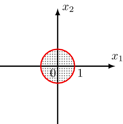
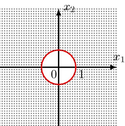
  ${\mathbb R}^n$. The radially symmetric regions can be a ball centred at the origin, the outside of this ball, and an annulus between two spheres. In dimension 2, we have sketched the graph of these three regions in figures 1–3. Of course, the most general radially symmetric regions can be a combination of the regions mentioned above. Since we can decompose the general radially symmetric regions into the above three regions and this decomposition allows us to analyse each region independently, in this work, we consider three regions:
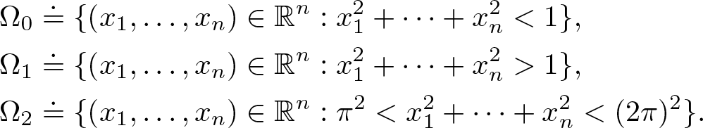 \begin{align*}
&\Omega_0
\doteq
\{
(x_1,\ldots,x_n)
\in
{\mathbb R}^n
:
x_1^2+\cdots+x_n^2 \lt 1
\},
\\
& \Omega_1
\doteq
\{
(x_1,\ldots,x_n)
\in
{\mathbb R}^n
:
x_1^2+\cdots+x_n^2 \gt 1
\},
\\
&\Omega_2
\doteq
\{
(x_1,\ldots,x_n)
\in
{\mathbb R}^n
:
\pi^2 \lt x_1^2+\cdots+x_n^2 \lt (2\pi)^2
\}.
\end{align*}
\begin{align*}
&\Omega_0
\doteq
\{
(x_1,\ldots,x_n)
\in
{\mathbb R}^n
:
x_1^2+\cdots+x_n^2 \lt 1
\},
\\
& \Omega_1
\doteq
\{
(x_1,\ldots,x_n)
\in
{\mathbb R}^n
:
x_1^2+\cdots+x_n^2 \gt 1
\},
\\
&\Omega_2
\doteq
\{
(x_1,\ldots,x_n)
\in
{\mathbb R}^n
:
\pi^2 \lt x_1^2+\cdots+x_n^2 \lt (2\pi)^2
\}.
\end{align*}Figures 1–3 depict the regions Ω0–Ω2, respectively, for the case of n = 2.
Equation (1.1a) can be classified as either focusing (indicated by the ‘λ > 0’) or defocusing (indicated by the ‘λ < 0’). When p = 4, it becomes the well-known cubic NLS equation ( $\lambda = \pm 1$)
 \begin{equation}
iu_t+u_{xx} \pm |u|^2 u
=
0,
\end{equation}
\begin{equation}
iu_t+u_{xx} \pm |u|^2 u
=
0,
\end{equation}which is a ubiquitous model in various areas of mathematical physics, including water waves, plasmas, optics, and Bose–Einstein condensates. The cubic NLS equation has been rigorously derived for water waves of small amplitude over infinite or finite depth and in the context of nonlinear optics [Reference Benney and Newell2, Reference Chiao, Garmire and Townes15, Reference Talanov33]. It has also been proposed as a model for rogue waves [Reference Chabchoub, Hoffmann and Akhmediev14, Reference Peregrine31]. In addition to its physical significance, the cubic NLS equation exhibits a complex mathematical framework as the archetypal illustration of a fully integrable system in one dimension. It features an unbounded hierarchy of symmetries and laws of conservation. In the one-dimensional case, the equation’s integrability is particularly noteworthy, as characterized by the existence of a Lax pair of the form:
Region Ω0.
Region Ω1.
Region Ω2.

 \begin{align}
\Psi_x
=
\left(
\begin{array}{lr}
-ik & u
\\
\mp \frac{1}{2}\bar u & ik
\end{array}
\right)
\Psi,
\quad
\Psi_t
=
\left(
\begin{array}{lr}
-2ik^2\pm\frac{i}{2}|u|^2 & 2ku+iu_x
\\
\mp k \bar u\pm\frac{i}{2}\bar u_x &2ik^2\mp\frac{i}{2}|u|^2
\end{array}
\right)
\Psi, \quad k\in\mathbb C.
\end{align}
\begin{align}
\Psi_x
=
\left(
\begin{array}{lr}
-ik & u
\\
\mp \frac{1}{2}\bar u & ik
\end{array}
\right)
\Psi,
\quad
\Psi_t
=
\left(
\begin{array}{lr}
-2ik^2\pm\frac{i}{2}|u|^2 & 2ku+iu_x
\\
\mp k \bar u\pm\frac{i}{2}\bar u_x &2ik^2\mp\frac{i}{2}|u|^2
\end{array}
\right)
\Psi, \quad k\in\mathbb C.
\end{align} The Lax pair formulation (1.3) allows the study of the initial value problem (ivp) for the cubic NLS equation under the assumption of initial data with sufficient smoothness and decay at infinity using the inverse scattering transform method [Reference Zakharov and Shabat36]. Well-posedness of the ivp for the NLS equation on the circle in Sobolev spaces Hs with  $s\geqslant 0$ has been proven by Bourgain [Reference Bourgain8] using modern harmonic analysis techniques. Earlier results include the works of Cazenave and Weissler [Reference Cazenave and Weissler13], Ginibre and Velo [Reference Ginibre and Velo22], Kenig, Ponce and Vega [Reference Kenig, Ponce and Vega29], and Tsutsumi [Reference Tsutsumi34]. In addition, the sharp well-posedness result on ${\mathbb R}$ was recently established in [Reference Harrop-Griffiths, Killip and Visan24].
Boundary value problems are particularly significant in real-world applications. For example, in the work [Reference Kamchatnov and Shchesnovich28], the authors study the dynamics of Bose–Einstein condensates confined in cigar-shaped traps, where the trap’s edges impose the boundary conditions. Although ibvps for Eq. (1.1a) are more relevant to real-world applications, they have received relatively little attention due in part to the lack of a Fourier transform in the case of bounded or semi-bounded spatial domains, which poses a significant obstacle to their analysis for dispersive equations like NLS and Korteweg-de Vries (KdV)equations. Nonetheless, researchers have explored various approaches to studying the ibvps, such as using the Riemann–Liouville fractional integration operator [Reference Colliander and Kenig18, Reference Holmer25], the Laplace transform [Reference Bona, Sun and Zhang5–Reference Bona, Sun and Zhang7], and the Fokas unified transform method [Reference Fokas, Himonas and Mantzavinos20, Reference Fokas, Himonas and Mantzavinos21]. Additionally, the ibvp of NLS in two dimensions has been studied in [Reference Himonas and Mantzavinos27, Reference Ran, Sun and Zhang32]. The regularity properties for the cubic NLS equations on the half-line are discussed in [Reference Erdoǧan and Tzirakis19] and the global well-posedness in one-dimensional spaces is addressed in [Reference Bona, Sun and Zhang7]. However, the corresponding ibvps for Eq. (1.1a) in bounded regions of higher dimension have not been explored and the goal of this article is to delve into this uncharted territory and establish a foundation for understanding the solution behaviour in more complex and realistic settings.
Here, we investigate the ibvp in  $\Omega_j, j=0,1,2$, which are radially symmetric regions of ${\mathbb R}^n$. We assume that the initial condition u 0 satisfies the following condition of radial symmetry:
 \begin{equation}
u_0(x_1,\ldots,x_n)
=
u_0(r),
\quad
\text{where}
\quad
r=\sqrt{x_1^2+\cdots+x_n^2}.
\end{equation}
\begin{equation}
u_0(x_1,\ldots,x_n)
=
u_0(r),
\quad
\text{where}
\quad
r=\sqrt{x_1^2+\cdots+x_n^2}.
\end{equation}We seek to find radially symmetric solutions of the ibvp. We equip the ibvp with different boundary conditions in three different domains. In Ω0, we use the boundary condition:
 \begin{equation}
u(x_1,\ldots,x_n,t)
=
g_2(t),
\quad
x_1^2+\cdots+x_n^2
=
1,
\,\,
t\in(0,T).
\end{equation}
\begin{equation}
u(x_1,\ldots,x_n,t)
=
g_2(t),
\quad
x_1^2+\cdots+x_n^2
=
1,
\,\,
t\in(0,T).
\end{equation}In Ω1, we use the boundary condition:
 \begin{equation}
u(x_1,\ldots,x_n,t)
=
g(t),
\quad
x_1^2+\cdots+x_n^2
=
1,
\,\,
t\in(0,T).
\end{equation}
\begin{equation}
u(x_1,\ldots,x_n,t)
=
g(t),
\quad
x_1^2+\cdots+x_n^2
=
1,
\,\,
t\in(0,T).
\end{equation}In Ω2, we use the boundary condition:
 \begin{align}
\begin{cases}
u(x_1,\ldots, x_n,t)
=
g_1(t),
&
x_1^2+\cdots +x_n^2=\pi^2,
\,\,
t\in(0,T),
\\
u(x_1,\ldots, x_n,t)
=
g_2(t),
&
x_1^2+\cdots +x_n^2=(2\pi)^2,
\,\,
t\in(0,T).
\end{cases}
\end{align}
\begin{align}
\begin{cases}
u(x_1,\ldots, x_n,t)
=
g_1(t),
&
x_1^2+\cdots +x_n^2=\pi^2,
\,\,
t\in(0,T),
\\
u(x_1,\ldots, x_n,t)
=
g_2(t),
&
x_1^2+\cdots +x_n^2=(2\pi)^2,
\,\,
t\in(0,T).
\end{cases}
\end{align}In addition to these boundary conditions, we have established compatibility conditions for each of the problems:
 \begin{align}
&\text{The ibvp in}\,\, \Omega_0:
\quad
u_0(1)
=
g_2(0),
\quad
1 \lt s \lt 2,
\end{align}
\begin{align}
&\text{The ibvp in}\,\, \Omega_0:
\quad
u_0(1)
=
g_2(0),
\quad
1 \lt s \lt 2,
\end{align} \begin{align}
&\text{The ibvp in}\,\, \Omega_1:
\quad
u_0(1)
=
g(0),
\quad
\frac12 \lt s \lt \frac32,
\end{align}
\begin{align}
&\text{The ibvp in}\,\, \Omega_1:
\quad
u_0(1)
=
g(0),
\quad
\frac12 \lt s \lt \frac32,
\end{align} \begin{align}
&\text{The ibvp in}\,\, \Omega_2:
\quad
u_0(\pi)
=
g_1(0)
\quad
\text{and}
\quad
u_0(2\pi)
=
g_2(0)
,
\quad
\frac12 \lt s \lt 2.
\end{align}
\begin{align}
&\text{The ibvp in}\,\, \Omega_2:
\quad
u_0(\pi)
=
g_1(0)
\quad
\text{and}
\quad
u_0(2\pi)
=
g_2(0)
,
\quad
\frac12 \lt s \lt 2.
\end{align} Furthermore, it is important to highlight that in this article, the lifespan  $T^*$ satisfies $0 \lt T^*\le T \lt \frac12$, and it depends on both the norm of initial data and the norm of boundary data. In addition, in the theorems that follow, the solutions are radially symmetric. With these clarifications, we can now present the primary outcomes and conclusions of our study.
In the following,  $H^s (\Omega )$ is denoted as the classical L 2-based Sobolev space in Ω with Sobolev inex s and $H^s_0 (\Omega )$ is the subspace of $H^2(\Omega )$ which is the closure of functions in $H^s (\Omega )$ with compact supports in Ω (formal definitions of those spaces will be given in §2).
Theorem 1.1 Let n = 2. Suppose  $u_0 \in H_0^s(\Omega_0)$, satisfying condition (1.4), and $g_2 \in H_0^{\frac{s+1}{2}}(0,T)$. If $1 \lt s \lt 2$, $p \geq 3$ and p is an even integer, then the ibvp within domain Ω0, subject to the compatibility condition (1.8a), is locally well-posed in $C( [0, T^*]; H^s(\Omega_0))$, where the lifespan $T^*$ depends on $\|u_0\|_{H^s(\Omega_0)}$, $\|g_2\|_{H^{\frac{s+1}{2}}(0,T)}$ and p.
Here, the use of spaces  $H^s_0 (\Omega_0)$ and $H_0^{\frac{s+1}{2}}(0,T)$ for initial and boundary data merely makes the proof of theorem 1.1 slightly more straightforward since the compatibility conditions for the initial and boundary data are automatically satisfied.
Theorem 1.2 Let  $n\ge 2$, $u_0\in H^s(\Omega_1)$, which satisfies the condition (1.4), and $g\in H^{\frac{2s+1}{4}}(0,T)$.
• If $0\le s \lt \frac12$ and $3\le p \lt \frac{6-4s}{1-2s}$, then the ibvp in domain Ω1 is locally well-posed in $C( [0, T^*]; H^s(\Omega_1))$.
• If
$\frac12 \lt s \lt \frac32$ and $p\ge 3$, then the ibvp in domain Ω1 with compatibility condition (1.8b) is locally well-posed in $C( [0, T^*]; H^s(\Omega_1))$.


In both cases, the lifespan  $T^*$ depends on $\|u_0\|_{H^s(\Omega_1)}$, $\|g\|_{H^{\frac{s+1}{4}}(0,T)}$ and p.
Theorem 1.3 Let  $n\ge 2$, $u_0\in H^s(\Omega_2)$, which satisfies the condition (1.4), $g_1\in H^{\frac{s+1}{2}}(0,T)$ and $g_2\in H^{\frac{s+1}{2}}(0,T)$.
• If
$0\le s \lt \frac12$ and $3\le p\le 4$, then the ibvp in domain Ω1 is locally well-posed in $C( [0, T^*]; H^s(\Omega_2))$.• If
$\frac12 \lt s \lt 2$, $s\neq \frac32$ and $p\ge 3$, then the ibvp in domain Ω2 with compatibility condition (1.8c) is locally well-posed in $C( [0, T^*]; H^s(\Omega_2))$.


In both cases, the lifespan  $T^*$ depends on $\|u_0\|_{H^s(\Omega_2)}$, $\|g_1\|_{H^{\frac{s+1}{2}}(0,T)}$, $\|g_2\|_{H^{\frac{s+1}{2}}(0,T)}$ and p.
We remark that the above theorems address a notable gap in current research, which is significantly important in the study of non-homogeneous boundary value problems for the NLS equations. In particular, theorem 1.2 gives an optimal regularity of the boundary data for the ibvp of NLS equations in Ω1, while theorems 1.1 and 1.3 provide the first account on the well-posedness issue for the ibvp of NLS equations in bounded regions of higher dimensions. Thus, the results in the article contribute to the limited body of knowledge on the ibvp of NLS equations and add valuable insights to the field, shedding light on a previously under-studied aspect of NLS equations, which we believe will be instrumental to the future research. Moreover, we note that the global well-posedness of ibvps in one-dimensional spaces has been addressed in [Reference Bona, Sun and Zhang7], though it imposes some restrictions on the nonlinearity. For the problems studied in this article, the global well-posedness can be analysed similarly with restrictions on the nonlinearity, utilizing energy conservation and boundary data estimates.
For s < 0, [Reference Christ, Colliander and Tao17] showed that the ivp for the cubic NLS equation is ill-posed because the mapping from initial data to solutions fails to be uniformly continuous. For the ibvp in the regions Ω1 and Ω2, we reduce this problem to the one-dimensional ibvp and prove well-posedness holds for  $s \ge 0$. Therefore, in terms of the uniform continuity of the data-to-solution map, theorems 1.2 and 1.3 are sharp. However, in the recent work [Reference Harrop-Griffiths, Killip and Visan24], the ivp for the cubic NLS equation was shown to be well-posed for $s \gt -\frac{1}{2}$, which is sharp. We have not yet achieved this sharp result for the ibvp, but we aim to explore this in future work.
Regarding the ibvp in the region Ω0, the non-zero boundary conditions complicate the derivation of Strichartz estimates. Thus, in theorem 1.1, we only establish local well-posedness for s > 1. The absence of these Strichartz estimates limits the sharpness of our result.
For the unforced case with zero boundary conditions, global well-posedness results have been achieved. In [Reference Bourgain and Bulut9, Reference Bourgain and Bulut10], the authors proved global well-posedness for the ibvp of the NLS equation on the two-dimensional and three-dimensional unit balls for  $0 \lt s \lt \frac{1}{2}$, utilizing and thoroughly discussing Strichartz estimates.
Additionally, in [Reference Blair, Smith and Sogge4], Strichartz estimates were established for the Schrödinger equation on Riemannian manifolds  $(\Omega, g)$ with zero boundary conditions. This applies both to compact cases and when Ω is the exterior of a smooth, non-trapping obstacle in Euclidean space. Using these estimates, the Schrödinger equation was shown to be well-posed in $H^1(\Omega)$ for three-dimensional space (see theorems 5.1 and 6.3 in [Reference Blair, Smith and Sogge4]).
Here, we note that although the works [Reference Blair, Smith and Sogge4, Reference Bourgain and Bulut9, Reference Bourgain and Bulut10] indeed derive Strichartz estimates for problems with zero boundary conditions, our study focuses on the ibvps with non-zero boundary conditions. The Strichartz estimates available in those literatures do not directly apply to such ibvps, which involve boundary integral operators, and as a result, there is a lack of established estimates for the cases we consider. This distinction is crucial to the novelty and challenges for the problem considered here.
In this article, we have not been able to derive the necessary Strichartz estimates for the boundary integral operator  $W_{ball}h$ defined by (5.27), which are required to prove the local well-posedness of the ibvp in the region Ω0. Hence, the presence of non-zero boundary conditions complicates the derivation of Strichartz estimates, and local well-posedness can only be achieved for s > 1. However, we have gained insights from the works mentioned above and plan to explore this direction further in future research.
Next, we provide an overview of the proof of the main results, which is comprised of four essential steps:
• Step 1. We begin by reducing the ibvp (1.1) to the NLS equation in one dimension when
$\Omega = \Omega_1$ or $\Omega = \Omega_2$. For $\Omega = \Omega_0$, due to the singularity at r = 0 if changing the equation in one dimension, we still use Ω0 in $\mathbb {R}^n$.• Step 2. We derive a solution formula for the corresponding linear forced ibvp, which will be crucial in obtaining estimates for the linear problem.
• Step 3. Using classical analysis, we obtain linear estimates for the data and forcing in suitable function spaces, which we refer to as ‘good’ solution spaces.
• Step 4. We prove that the iteration map defined by the solution formula, with the forcing replaced by the nonlinearity, is a contraction in ‘good’ solution spaces. This will allow us to use the contraction mapping principle to establish the existence of a unique solution to the nonlinear problem.


Here, we remark that, since the solutions and the domains are radially symmetric, we may change the ibvps for  $\Omega = \Omega_1$ or Ω2 to 1D NLS equations on a half line or a finite interval with one or two boundary points. These 1D problems have been studied in [Reference Bona, Sun and Zhang7, Reference Fokas, Himonas and Mantzavinos21]. If we require certain linear estimates from [Reference Bona, Sun and Zhang7, Reference Fokas, Himonas and Mantzavinos21] in our proof, we may either cite them or provide shorter or more elegant proof.
Paper organization: In §2, we introduce crucial preliminary results that are foundational for our subsequent proofs. Section 3 is dedicated to establishing the well-posedness result for regions outside a ball, with a specific focus on proving theorem 1.2. In §4, we delve into the well-posedness result within an annulus and provide the proof for theorem 1.3. Section 5 is dedicated to demonstrating the well-posedness result within a ball centred at the origin, presenting the proof for theorem 1.1. Additionally, we include an Appendix section where we provide proofs that may have been omitted in earlier sections.
2. Preliminary
In this section, since we only consider the solutions of (1.1) with radial form, we rewrite (1.1) as
 \begin{align}
&iu_t+
u_{rr} + \frac{n-1}{r} u_r +\lambda|u|^{p-2} u = 0,
& &r \in (r_1, r_2),\,\,t\in(0,T),
\end{align}
\begin{align}
&iu_t+
u_{rr} + \frac{n-1}{r} u_r +\lambda|u|^{p-2} u = 0,
& &r \in (r_1, r_2),\,\,t\in(0,T),
\end{align} \begin{align}
&u(r ,0)
=
u_0(r ),
& &r \in (r_1, r_2),
\end{align}
\begin{align}
&u(r ,0)
=
u_0(r ),
& &r \in (r_1, r_2),
\end{align} \begin{align}
&u(r_1,t)
=
g_1(t)\, , \qquad u(r_2,t)
=
g_2(t),
&
&
t\in(0,T),
\end{align}
\begin{align}
&u(r_1,t)
=
g_1(t)\, , \qquad u(r_2,t)
=
g_2(t),
&
&
t\in(0,T),
\end{align} where  $r_1, r_2 $ are chosen appropriately for $\Omega_j , j = 0, 1, 2$ and $r=(x_1^2+\dots+x_n^2)^{\frac{1}{2}}$. Here,
 \begin{align}
\Delta u
=
\partial_{x_1}^2u+\cdots+\partial_{x_n}^2u
=
u''(r)+\frac{n-1}{r}u'(r)
\end{align}
\begin{align}
\Delta u
=
\partial_{x_1}^2u+\cdots+\partial_{x_n}^2u
=
u''(r)+\frac{n-1}{r}u'(r)
\end{align}has been used.
The corresponding linear ibvp is
 \begin{align}
&iu_t
+
u_{rr} + \frac{n-1}{r} u_r = f(r,t),
& &
r \in (r_1, r_2),
\,\,
t\in(0,T),
\end{align}
\begin{align}
&iu_t
+
u_{rr} + \frac{n-1}{r} u_r = f(r,t),
& &
r \in (r_1, r_2),
\,\,
t\in(0,T),
\end{align} \begin{align}
&u(r,0)
=
u_0(r),
& &
r \in (r_1, r_2),
\end{align}
\begin{align}
&u(r,0)
=
u_0(r),
& &
r \in (r_1, r_2),
\end{align} \begin{align}
&u(r_1,t)
=
g_1(t)\, , \qquad u(r_2,t)
=
g_2(t),
&
&
t\in(0,T).
\end{align}
\begin{align}
&u(r_1,t)
=
g_1(t)\, , \qquad u(r_2,t)
=
g_2(t),
&
&
t\in(0,T).
\end{align} If  $r_1\not = 0$, we can use a change of dependent variable $u(r,t)=r^{-\frac{n-1}{2}}\cdot v(r,t)$ to derive the equations for v, that is
 \begin{align}
&iv_t+v_{rr}=r^{\frac{n-1}2}f(r,t)+\frac{n^2-4n+3}{4}r^{-2}\cdot v,
& &
r \in (r_1, r_2),
\,\,
t\in(0,T),
\end{align}
\begin{align}
&iv_t+v_{rr}=r^{\frac{n-1}2}f(r,t)+\frac{n^2-4n+3}{4}r^{-2}\cdot v,
& &
r \in (r_1, r_2),
\,\,
t\in(0,T),
\end{align} \begin{align}
&v(r,0)
=
r^{\frac{n-1}2}u_0(r) = v_0 (r),
& &
r \in (r_1, r_2),
\end{align}
\begin{align}
&v(r,0)
=
r^{\frac{n-1}2}u_0(r) = v_0 (r),
& &
r \in (r_1, r_2),
\end{align} \begin{align}
&v(r_1,t)
=
r_1^{\frac{n-1}{2}}g_1(t)\, , \qquad v(r_2,t)
=
r_2^{\frac{n-1}{2}}g_2(t),
&
&
t\in(0,T).
\end{align}
\begin{align}
&v(r_1,t)
=
r_1^{\frac{n-1}{2}}g_1(t)\, , \qquad v(r_2,t)
=
r_2^{\frac{n-1}{2}}g_2(t),
&
&
t\in(0,T).
\end{align} From the theory of the ivp (1.1) in  $\mathbb{R}^n$, it is known that if the initial data u 0 of radial form is in $W^{s,2}(\Omega_j ), j = 0, 1,2$, then $u_0 (r) $ is in $W^{s,2}_{r^{n-1}}(r_1,r_2)$ for $r _1 \not = 0 $, which implies that $v_0 ( r ) \in W^{s, 2} ( r_1 , r_2 ) $. Here, the weighted Sobolev space $W_\omega^{m,p}$ over the open region Ω is given by (see [Reference Turesson35]),
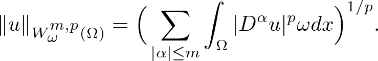 \begin{align}
\|u\|_{W_\omega^{m,p}(\Omega)}
=
\Big(
\sum\limits_{|\alpha|\le m}
\int_{\Omega}
|D^{\alpha} u|^p
\omega
dx
\Big)^{1/p}.
\end{align}
\begin{align}
\|u\|_{W_\omega^{m,p}(\Omega)}
=
\Big(
\sum\limits_{|\alpha|\le m}
\int_{\Omega}
|D^{\alpha} u|^p
\omega
dx
\Big)^{1/p}.
\end{align} Hence, we only need to discuss the solutions of (2.4) in L 2-based Sobolev spaces if  $r_1 \not = 0$.
If  $r_1 = 0 $, then the above change of dependent variables introduces a singularity at r = 0 and cannot be used, which implies that the weighted Sobolev spaces are necessary. For the case that $r_2 = \infty$, the problem (2.1) is the NLS equation posed in $\mathbb{R}^n$ with radial symmetric initial data. If we consider the following ivp of linear Schrödinger equation
 \begin{align}
&iU_t+\Delta U
=
F,
& &(x_1,\ldots,x_n)\in {\mathbb R}^n,\,\,t\in(0,T),
\end{align}
\begin{align}
&iU_t+\Delta U
=
F,
& &(x_1,\ldots,x_n)\in {\mathbb R}^n,\,\,t\in(0,T),
\end{align} \begin{align}
&U(x_1,\ldots,x_n,0)
=
U_0(x_1,\ldots, x_n),
& &(x_1,\ldots, x_n)\in {\mathbb R}^n\,,
\end{align}
\begin{align}
&U(x_1,\ldots,x_n,0)
=
U_0(x_1,\ldots, x_n),
& &(x_1,\ldots, x_n)\in {\mathbb R}^n\,,
\end{align}then using Fourier transform, we have
 \begin{align}
U
=
S_n[U_0;F]
\doteq&
\frac{1}{(2\pi)^n}
\int_{{\mathbb R}^n}
e^{i\xi \cdot x-i|\xi|^2t}
\widehat{U}_0(\xi_1,\ldots,\xi_n)
d\xi_1\cdots d\xi_n
\end{align}
\begin{align}
U
=
S_n[U_0;F]
\doteq&
\frac{1}{(2\pi)^n}
\int_{{\mathbb R}^n}
e^{i\xi \cdot x-i|\xi|^2t}
\widehat{U}_0(\xi_1,\ldots,\xi_n)
d\xi_1\cdots d\xi_n
\end{align} \begin{align}
-&
\frac{i}{(2\pi)^n}
\int_0^t
\int_{{\mathbb R}^n}
e^{i\xi \cdot x-i|\xi|^2(t-t')}
\widehat{F}^{x}(\xi_1,\ldots,\xi_n,t')
d\xi_1\cdots d\xi_n
dt',
\end{align}
\begin{align}
-&
\frac{i}{(2\pi)^n}
\int_0^t
\int_{{\mathbb R}^n}
e^{i\xi \cdot x-i|\xi|^2(t-t')}
\widehat{F}^{x}(\xi_1,\ldots,\xi_n,t')
d\xi_1\cdots d\xi_n
dt',
\end{align} where  $\xi\cdot x=\xi_1x_1+\cdots+\xi_nx_n$ and $|\xi|^2=\xi_1^2+\cdots+\xi_n^2$. Also, we have following claim.
Claim. If U 0 and F are radially symmetric, that is, for  $r\ge 0$ we have
 \begin{align*}
U_0(x_1,\ldots, x_n)
=
U_0(r),
\quad
F(x_1,\ldots, x_n,t)
=
F(r,t),
\quad
x_1^2+\cdots+x_n^2
=
r^2,
\end{align*}
\begin{align*}
U_0(x_1,\ldots, x_n)
=
U_0(r),
\quad
F(x_1,\ldots, x_n,t)
=
F(r,t),
\quad
x_1^2+\cdots+x_n^2
=
r^2,
\end{align*}then the solution of the above ivp (2.6) is also radially symmetric.
Proof. The above claim follows from the next result.
Lemma 2.1. If f is radially symmetric, then  $\widehat{f}$ is also radially symmetric. Conversely, if $\widehat{f}$ is radially symmetric, then f is radially symmetric.
Now, since the term (2.7a) is the inverse Fourier transform of  $e^{-i|\xi|^2t}
\widehat{U}_0(\xi_1,\ldots,\xi_n)$, by lemma 2.1, the term (2.7a) is radially symmetric. Similarly, since term (2.7b) is the integral of the inverse Fourier transform
$e^{-i|\xi|^2t}
\widehat{U}_0(\xi_1,\ldots,\xi_n)$, by lemma 2.1, the term (2.7a) is radially symmetric. Similarly, since term (2.7b) is the integral of the inverse Fourier transform  $e^{-i|\xi|^2(t-t')}
\widehat{F}(\xi_1,\ldots,\xi_n,t')$, lemma 2.1 implies that this term is also radially symmetric. This completes the claim.
$e^{-i|\xi|^2(t-t')}
\widehat{F}(\xi_1,\ldots,\xi_n,t')$, lemma 2.1 implies that this term is also radially symmetric. This completes the claim.
Proof of lemma 2.1
Here, we only prove that the Fourier transform of a radially symmetric function is radially symmetric. The Fourier transform of function f(x) in  $\mathbb{R}^n$ is defined as:
 \begin{align}
\widehat{f}(\xi)
=
\int_{\mathbb{R}^n} f(x) e^{-i\xi\cdot x} dx,
\end{align}
\begin{align}
\widehat{f}(\xi)
=
\int_{\mathbb{R}^n} f(x) e^{-i\xi\cdot x} dx,
\end{align} where  $\xi\cdot x = \xi_1 x_1 + \cdots + \xi_n x_n$ denotes the dot product of the vectors ξ and x. To show that $\widehat{f}(\xi)$ is also radially symmetric, we need to show that $\widehat{f}(\xi)$ is invariant under rotations, i.e., if we rotate the vector ξ in $\mathbb{R}^n$ by an angle θ, the Fourier transform $\widehat{f}(\xi)$ remains the same.
Let R be a rotation matrix in  $\mathbb{R}^n$, i.e., R is an n × n orthogonal matrix with determinant 1. Then, we have:
 \begin{align*}
\widehat{f}(R\xi)
=&
\int_{\mathbb{R}^n} f(r) e^{-i(R\xi)\cdot x} dx
=
\int_{\mathbb{R}^n} f(r) e^{-i\xi\cdot R^{-1} x} dx
\overset{y = R^{-1} x}{=}
\int_{\mathbb{R}^n} f(r) e^{-i\xi\cdot y} dy\\
=&
\widehat{f}(\xi),
\end{align*}
\begin{align*}
\widehat{f}(R\xi)
=&
\int_{\mathbb{R}^n} f(r) e^{-i(R\xi)\cdot x} dx
=
\int_{\mathbb{R}^n} f(r) e^{-i\xi\cdot R^{-1} x} dx
\overset{y = R^{-1} x}{=}
\int_{\mathbb{R}^n} f(r) e^{-i\xi\cdot y} dy\\
=&
\widehat{f}(\xi),
\end{align*} where we have used the fact that  $R^{-1}=R^T$ for an orthogonal matrix R.
Thus, we have shown that the Fourier transform of a radially symmetric function in  $\mathbb{R}^n$ is also radially symmetric, i.e., $\widehat{f}(\xi) = \widehat{f}(|\xi|)$. This completes the proof of lemma 2.1.
Therefore, by above discussion, we can use the well-posedness theory of the NLS equations in  $\mathbb{R}^n$ to establish the well-posedness of (2.1) with $r_1 = 0 $ and $r_2 = \infty$ under the assumption that $u_0 (r ) \in W^{s , 2 } _{r^{n-1}} (\mathbb{R}) $ with $s \geq 0$. We note that the boundary condition for (2.1) at r = 0 must be $v_r ( 0 ) = 0$ and the solution space is $ W^{s , 2 } _{r^{n-1}} (\mathbb{R}) $ with $s \geq 0$. Hence, in the following, we will only consider the cases with $ 0 \lt r_1 \lt r_2 = \infty$, $ 0 \lt r_1 \lt r_2 \lt \infty$, and $ 0 = r_1 \lt r_2 \lt \infty$.
Here, we recall the linear estimate for the solution  $S_n[U_0;F]$.
Proposition 2.2. [Strichartz estimates for linear Schrödinger equation]
For  $s\ge 0$, if $(q,\gamma)$ and $(q_1,\gamma_1)$ are admissible, which are given below in definition 2.3. Then the solution $U=S_n[U_0;F]$ of ivp (2.6) satisfies
 \begin{equation}
\big\|
S_n[U_0;F]
\big\|_{L^q(0,T; W^{s,\gamma}({\mathbb R}^n))}
\lesssim
\|U_0\|_{H^s({\mathbb R}^n)}
+
\big\|
F
\big\|_{L^{q_1'}(0,T; W^{s,\gamma_1'}({\mathbb R}^n))}.
\end{equation}
\begin{equation}
\big\|
S_n[U_0;F]
\big\|_{L^q(0,T; W^{s,\gamma}({\mathbb R}^n))}
\lesssim
\|U_0\|_{H^s({\mathbb R}^n)}
+
\big\|
F
\big\|_{L^{q_1'}(0,T; W^{s,\gamma_1'}({\mathbb R}^n))}.
\end{equation}The proof of proposition 2.2 can be found in [Reference Cazenave11] (see theorem 2.3.3).
Throughout this work, we shall use the familiar time localizer  $\psi(t)$, which is defined as follows:
 \begin{equation}
\psi \in C^{\infty}_0(-1, 1),
\,\,\,
0\le \psi \le 1
\,\,
\text{and }
\,\,
\psi(t)=1
\,\,
\text{for }
\,\,
|t|\le \frac12.
\end{equation}
\begin{equation}
\psi \in C^{\infty}_0(-1, 1),
\,\,\,
0\le \psi \le 1
\,\,
\text{and }
\,\,
\psi(t)=1
\,\,
\text{for }
\,\,
|t|\le \frac12.
\end{equation}Moreover, we introduce the notion of admissible pair
Definition 2.3. We say that a pair  $(q,\gamma)$ is admissible (in n dimension), if
 \begin{equation}
\frac{2}{q}+\frac{n}{\gamma}
=
\frac{n}{2},
\end{equation}
\begin{equation}
\frac{2}{q}+\frac{n}{\gamma}
=
\frac{n}{2},
\end{equation}and
 \begin{equation}
2\le\gamma\le\frac{2n}{n-2},
\qquad
(2\le \gamma\le \infty
\text{if } n=1,
\quad
2\le \gamma \lt \infty
\text{if } n=2)\, .
\end{equation}
\begin{equation}
2\le\gamma\le\frac{2n}{n-2},
\qquad
(2\le \gamma\le \infty
\text{if } n=1,
\quad
2\le \gamma \lt \infty
\text{if } n=2)\, .
\end{equation} Additionally, the Sobolev space  $H^s({\mathbb R}^n)$ consists of all temperate distributions F with the norm
 \begin{align}
\| F \|_{H^s({\mathbb R}^n)}
\doteq
\Big(
\int_{{\mathbb R}^n} (1+ |\xi|)^{2s}
|\widehat F(\xi)|^2 d\xi \Big)^{1/2},
\end{align}
\begin{align}
\| F \|_{H^s({\mathbb R}^n)}
\doteq
\Big(
\int_{{\mathbb R}^n} (1+ |\xi|)^{2s}
|\widehat F(\xi)|^2 d\xi \Big)^{1/2},
\end{align} where  $\widehat F(\xi)$ is the Fourier transform defined by
 \begin{equation*}
\widehat F(\xi)
\doteq
\int_{{\mathbb R}^n} e^{-i\xi\cdot x} F(x)dx.
\end{equation*}
\begin{equation*}
\widehat F(\xi)
\doteq
\int_{{\mathbb R}^n} e^{-i\xi\cdot x} F(x)dx.
\end{equation*} For an open set  $\Omega\subset {\mathbb R}^n$, the space $H^s(\Omega)$ is defined by
 \begin{equation}
H^s(\Omega)
\!\doteq\!
\big\{f\!:\! f\!=\! F\big|_{\Omega}\
\mathrm{where}\ F\!\in\! H^s({\mathbb R}^n)\
\mathrm{and}\
\| f \|_{H^s(\Omega)} \!\doteq\! \inf_{F \in H^s(\mathbb R^n)}
\| F \|_{H^s({\mathbb R}^n)} \! \lt \! \infty
\big\}.
\end{equation}
\begin{equation}
H^s(\Omega)
\!\doteq\!
\big\{f\!:\! f\!=\! F\big|_{\Omega}\
\mathrm{where}\ F\!\in\! H^s({\mathbb R}^n)\
\mathrm{and}\
\| f \|_{H^s(\Omega)} \!\doteq\! \inf_{F \in H^s(\mathbb R^n)}
\| F \|_{H^s({\mathbb R}^n)} \! \lt \! \infty
\big\}.
\end{equation} Here, we remind the reader that the space  $H_0^s(\Omega)$ is the subspace which is the closure of the class of functions in $H^s({\mathbb R}^n)$ whose support lies in Ω.
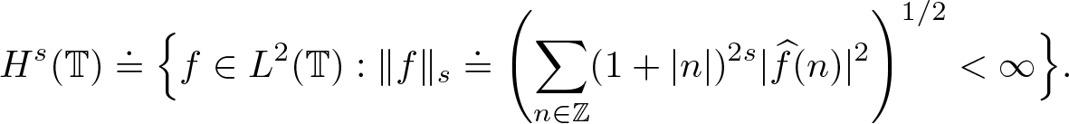
Finally, we define the Sobolev space on a torus, which will be used to study the problem on annulus. For  $s\ge 0$, the Sobolev space $H^s({\mathbb{T}})$ is defined by
 \begin{equation}
H^s(\mathbb{T})\doteq
\Big\{f\in L^2(\mathbb{T}):
\|f\|_{s}
\doteq
\left( \sum_{n \in\mathbb{Z}}
(1+|n|)^{2s} |\widehat{f}(n)|^2\right)^{1/2} \lt \infty
\Big\}.
\end{equation}
\begin{equation}
H^s(\mathbb{T})\doteq
\Big\{f\in L^2(\mathbb{T}):
\|f\|_{s}
\doteq
\left( \sum_{n \in\mathbb{Z}}
(1+|n|)^{2s} |\widehat{f}(n)|^2\right)^{1/2} \lt \infty
\Big\}.
\end{equation}Also, recall the Fourier transform
 \begin{equation}
\widehat{f}(n)=\int_{-\pi}^{\pi} e^{-inx}f(x)\, dx,\,
\quad
n\in\mathbb{Z},
\end{equation}
\begin{equation}
\widehat{f}(n)=\int_{-\pi}^{\pi} e^{-inx}f(x)\, dx,\,
\quad
n\in\mathbb{Z},
\end{equation}and the inverse Fourier transform
 \begin{equation}
f(x)
=
\frac{1}{2\pi}
\sum_{n\in\mathbb{Z}}\widehat{f}(n) e^{inx}.
\end{equation}
\begin{equation}
f(x)
=
\frac{1}{2\pi}
\sum_{n\in\mathbb{Z}}\widehat{f}(n) e^{inx}.
\end{equation} Equations (2.16) and (2.17) present identities that hold in the sense of distributions. Specifically, for functions f such that  $f\in L^1$, the Fourier transform $\hat{f}$ is in $\ell^1$, ensuring the validity of the identities as stated.
3. NLS equations on a half-line (i.e., outside of a ball)
In this section, we study (2.1) on a half-line with  $ r \in ( 1, \infty)$ (i.e., outside of a ball) and a boundary condition $u ( 1, t ) = g (t)$, where $r_1 = 1$ is chosen for the sake of convenience. We first discuss the corresponding linear problem and then obtain the well-posedness of the nonlinear problem.
3.1. Solutions of linear problems with estimates in Sobolev Spaces
If  $f_1(r,t)\doteq r^{\frac{n-1}2}f(r,t)+\frac{n^2-4n+3}{4}r^{-2}\cdot v$ and $v_0(r)=r^{\frac{n-1}2}u_0(r)$, then (2.4) becomes
 \begin{align}
&iv_t+v_{rr}=f_1(r,t),
& &
r \gt 1,
\,\,
t\in(0,T),
\end{align}
\begin{align}
&iv_t+v_{rr}=f_1(r,t),
& &
r \gt 1,
\,\,
t\in(0,T),
\end{align} \begin{align}
&v(r,0)
=
v_0(r),
& &
r \gt 1,
\end{align}
\begin{align}
&v(r,0)
=
v_0(r),
& &
r \gt 1,
\end{align} \begin{align}
&v(1,t)
=
g(t),
&
&
t\in(0,T).
\end{align}
\begin{align}
&v(1,t)
=
g(t),
&
&
t\in(0,T).
\end{align}Also, by using the compatibility (1.8b), the above ibvp is equipped with the following compatibility condition
 \begin{equation}
g(0)
=
v_0 (1) ,
\quad
\frac12 \lt s \lt \frac32.
\end{equation}
\begin{equation}
g(0)
=
v_0 (1) ,
\quad
\frac12 \lt s \lt \frac32.
\end{equation}Next, we solve the ibvp (3.1) and begin with decomposing the above ibvp into simpler problems. In fact, using superposition principle, the linear ibvp (3.1) can be expressed as the homogeneous ibvp
 \begin{align}
&iv_t+v_{rr}
=
0,
& &
r \gt 1,
\,\,t\in(0,T),
\end{align}
\begin{align}
&iv_t+v_{rr}
=
0,
& &
r \gt 1,
\,\,t\in(0,T),
\end{align} \begin{align}
&v(r,0)
=
v_0(r)\in H^s(1,\infty),
& &
r \gt 1,
\end{align}
\begin{align}
&v(r,0)
=
v_0(r)\in H^s(1,\infty),
& &
r \gt 1,
\end{align} \begin{align}
&v(1,t)
=
g(t)
\in
H^{\frac{2s+1}{4}}(0,T),
&&
t\in(0,T),
\end{align}
\begin{align}
&v(1,t)
=
g(t)
\in
H^{\frac{2s+1}{4}}(0,T),
&&
t\in(0,T),
\end{align}and the forced linear ibvp with zero initial and boundary data
 \begin{align}
&iv_t+v_{rr}
=
f_1(r,t),
& &r \gt 1,\,\,t\in(0,T),
\end{align}
\begin{align}
&iv_t+v_{rr}
=
f_1(r,t),
& &r \gt 1,\,\,t\in(0,T),
\end{align} \begin{align}
&v(r,0)
=
0,
& &r \gt 1,
\end{align}
\begin{align}
&v(r,0)
=
0,
& &r \gt 1,
\end{align} \begin{align}
&v(1,t)
=
0,
&
&
t\in(0,T).
\end{align}
\begin{align}
&v(1,t)
=
0,
&
&
t\in(0,T).
\end{align}Also, we can do further decomposition. In fact, the homogeneous ibvp (3.3) can be expressed as the homogeneous ivp and the pure ibvp. The homogeneous ivp is given by:
 \begin{align}
&iV_t+V_{rr}
=
0,
& &t\in(0,T),
\end{align}
\begin{align}
&iV_t+V_{rr}
=
0,
& &t\in(0,T),
\end{align} \begin{align}
&V(r,0)
=
V_0(r)\in H^s({\mathbb R}),
\end{align}
\begin{align}
&V(r,0)
=
V_0(r)\in H^s({\mathbb R}),
\end{align} where V 0 is the extension of v 0 from  $(1,\infty)$ to ${\mathbb R}$ such that
 \begin{equation}
\|V_0\|_{H^s({\mathbb R})}
\le
2
\|v_0\|_{H^s(1,\infty)}.
\end{equation}
\begin{equation}
\|V_0\|_{H^s({\mathbb R})}
\le
2
\|v_0\|_{H^s(1,\infty)}.
\end{equation}The pure ibvp is given by:
 \begin{align}
&iv_t+v_{rr}
=
0,
& &r \gt 1,\,\,t\in(0,T),
\end{align}
\begin{align}
&iv_t+v_{rr}
=
0,
& &r \gt 1,\,\,t\in(0,T),
\end{align} \begin{align}
&v(r,0)
=
0,
& &r \gt 1,
\end{align}
\begin{align}
&v(r,0)
=
0,
& &r \gt 1,
\end{align} \begin{align}
&v(1,t)
=
g(t)-V(1,t)
\in
H^{\frac{2s+1}{4}}(0,T),
&&
t\in(0,T).
\end{align}
\begin{align}
&v(1,t)
=
g(t)-V(1,t)
\in
H^{\frac{2s+1}{4}}(0,T),
&&
t\in(0,T).
\end{align}For the inhomogeneous ibvp (3.4), it can be decomposed as a forced ivp and a pure ibvp:
 \begin{align}
&iW_t+W_{rr}
=
F(r,t),
& &r \gt 1,\,\,t\in(0,T),
\end{align}
\begin{align}
&iW_t+W_{rr}
=
F(r,t),
& &r \gt 1,\,\,t\in(0,T),
\end{align} \begin{align}
&W(r,0)
=
0,
\end{align}
\begin{align}
&W(r,0)
=
0,
\end{align} where F is the extension of f 1 from  $(1,\infty)$ to ${\mathbb R}$ such that
 \begin{equation}
\|F\|_{L_t^{q'}(0,T; W^{s,\gamma'}({\mathbb R}))}
\le
2
\|f_1\|_{L_t^{q'}(0,T; W^{s,\gamma'}(1,\infty))}.
\end{equation}
\begin{equation}
\|F\|_{L_t^{q'}(0,T; W^{s,\gamma'}({\mathbb R}))}
\le
2
\|f_1\|_{L_t^{q'}(0,T; W^{s,\gamma'}(1,\infty))}.
\end{equation}The pure ibvp is given by:
 \begin{align}
&iv_t+v_{rr}
=
0,
& &r \gt 1,\,\,t\in(0,T),
\end{align}
\begin{align}
&iv_t+v_{rr}
=
0,
& &r \gt 1,\,\,t\in(0,T),
\end{align} \begin{align}
&v(r,0)
=
0,
& &r \gt 1,
\end{align}
\begin{align}
&v(r,0)
=
0,
& &r \gt 1,
\end{align} \begin{align}
&v(1,t)
=
-W(1,t)
&&
t\in(0,T).
\end{align}
\begin{align}
&v(1,t)
=
-W(1,t)
&&
t\in(0,T).
\end{align}Linear estimate for homogeneous ivp (3.5). The solution to this problem is obtained by Fourier transform
 \begin{align}
V(r,t)
=
S[V_0; 0](r,t)
\doteq
\frac{1}{2\pi}
\int_{{\mathbb R}}
e^{i\xi r-i\xi^2t}
\widehat{V}_0(\xi)
d\xi,
\end{align}
\begin{align}
V(r,t)
=
S[V_0; 0](r,t)
\doteq
\frac{1}{2\pi}
\int_{{\mathbb R}}
e^{i\xi r-i\xi^2t}
\widehat{V}_0(\xi)
d\xi,
\end{align} where  $\widehat{V}_0$ is the Fourier transform of V 0, that is
 \begin{equation*}
\widehat{V}_0
\doteq
\int_{\mathbb R}
e^{-i\xi r}
V_0(r)
dr.
\end{equation*}
\begin{equation*}
\widehat{V}_0
\doteq
\int_{\mathbb R}
e^{-i\xi r}
V_0(r)
dr.
\end{equation*} We have the following estimates for  $S[V_0; 0]$, whose proof can be found in [Reference Cazenave and Haraux12, Reference Holmer25].
Proposition 3.1. Homogeneous ivp estimates
The solution  $V=S[V_0; 0]$ of the homogeneous linear Schrödinger ivp (3.5) given by formula (3.11) satisfies the space estimate:
 \begin{align}
\sup\limits_{t\in[0,T]}
\|
S[V_0; 0](t)
\|_{H^s({\mathbb R})}
=
\|
V_0
\|_{H^s({\mathbb R})},
\quad
s\in{\mathbb R}.
\end{align}
\begin{align}
\sup\limits_{t\in[0,T]}
\|
S[V_0; 0](t)
\|_{H^s({\mathbb R})}
=
\|
V_0
\|_{H^s({\mathbb R})},
\quad
s\in{\mathbb R}.
\end{align} Also,  $S[V_0;0]$ satisfies the time estimate
 \begin{align}
\sup\limits_{r\in{\mathbb R}}
\|
S[V_0; 0](r)
\|_{H^{\frac{2s+1}{4}}(0,T)}
\lesssim
\|
V_0
\|_{H^s({\mathbb R})},
\quad
s\in{\mathbb R}.
\end{align}
\begin{align}
\sup\limits_{r\in{\mathbb R}}
\|
S[V_0; 0](r)
\|_{H^{\frac{2s+1}{4}}(0,T)}
\lesssim
\|
V_0
\|_{H^s({\mathbb R})},
\quad
s\in{\mathbb R}.
\end{align} In addition, if  $\frac{2}{q}+\frac{1}{\gamma}=\frac12$ and $\gamma\ge 2$, then $S[V_0; 0](r,t)$ satisfies the following Strichartz estimate
 \begin{align}
\|
S[V_0; 0]
\|_{L_t^q({\mathbb R}; W^{s,\gamma}({\mathbb R}))}
\lesssim
\|
V_0
\|_{H^s({\mathbb R})},
\quad
s\ge 0.
\end{align}
\begin{align}
\|
S[V_0; 0]
\|_{L_t^q({\mathbb R}; W^{s,\gamma}({\mathbb R}))}
\lesssim
\|
V_0
\|_{H^s({\mathbb R})},
\quad
s\ge 0.
\end{align}Linear estimate for forced ivp (3.8). The solution to this problem is given by
 \begin{align}
W
=
S[0; F](r,t)
\doteq &
-\frac{i}{2\pi}
\int_{t'=0}^t
\int_{{\mathbb R}}
e^{i\xi r-i\xi^2(t-t')}
\widehat{F}^r(\xi, t')
d\xi
dt'
\end{align}
\begin{align}
W
=
S[0; F](r,t)
\doteq &
-\frac{i}{2\pi}
\int_{t'=0}^t
\int_{{\mathbb R}}
e^{i\xi r-i\xi^2(t-t')}
\widehat{F}^r(\xi, t')
d\xi
dt'
\end{align} \begin{align}
=&
-i\int_{t'=0}^t
S[F(\cdot,t');0]
(r,t-t')
dt'\, ,
\end{align}
\begin{align}
=&
-i\int_{t'=0}^t
S[F(\cdot,t');0]
(r,t-t')
dt'\, ,
\end{align} where  $\widehat{F}^r$ is the Fourier transform of F and $S[F(\cdot,t');0]$ denotes the solution of homogeneous ivp (3.5) with initial datum $F(r,t')$. We have the following estimates for $S[0; F](r,t)$, whose proof also can be found in [Reference Cazenave and Haraux12, Reference Holmer25]
Proposition 3.2. Forced ivp estimates
The solution  $W=S[0; F]$ of the forced ivp (3.8) given by formula (3.15) satisfies the space estimate:
 \begin{align}
\sup\limits_{t\in[0,T]}
\|
S[0; F](t)
\|_{H^s({\mathbb R})}
\le
T
\sup\limits_{t\in[0,T]}
\|
F(t)
\|_{H^s({\mathbb R})},
\quad
s\in{\mathbb R}.
\end{align}
\begin{align}
\sup\limits_{t\in[0,T]}
\|
S[0; F](t)
\|_{H^s({\mathbb R})}
\le
T
\sup\limits_{t\in[0,T]}
\|
F(t)
\|_{H^s({\mathbb R})},
\quad
s\in{\mathbb R}.
\end{align} Also,  $S[0;F]$ satisfies the time estimate
 \begin{align}
&\sup_{r\in \mathbb R}\|S[0;F](r)\|_{H_t^{\frac{2s+1}{4}}(0,T)}
\lesssim
(1+T)^{\frac14}
\|
F
\|_{L_t^{q'}(0,T; W^{s,\gamma'}({\mathbb R}))},
\quad
-\frac12 \lt s \lt \frac12,
\end{align}
\begin{align}
&\sup_{r\in \mathbb R}\|S[0;F](r)\|_{H_t^{\frac{2s+1}{4}}(0,T)}
\lesssim
(1+T)^{\frac14}
\|
F
\|_{L_t^{q'}(0,T; W^{s,\gamma'}({\mathbb R}))},
\quad
-\frac12 \lt s \lt \frac12,
\end{align} \begin{align}
&\sup_{r\in {\mathbb R}}\|S[0;F](r)\|_{H_t^{\frac{2s+1}{4}}(0,T)}
\lesssim
\big\|F\big\|_{L^1\big(0,T; H^s({\mathbb R})\big)},
\quad
\frac12 \lt s \lt \frac32.
\end{align}
\begin{align}
&\sup_{r\in {\mathbb R}}\|S[0;F](r)\|_{H_t^{\frac{2s+1}{4}}(0,T)}
\lesssim
\big\|F\big\|_{L^1\big(0,T; H^s({\mathbb R})\big)},
\quad
\frac12 \lt s \lt \frac32.
\end{align} In addition, if  $\frac{2}{q}+\frac{1}{\gamma}=\frac12$, and $\gamma\ge 2$, then $S[0; F](r,t)$ satisfies the following Strichartz estimate
 \begin{align}
\|
S[0; F]
\|_{L_t^q(0,T; W^{s,\gamma}({\mathbb R}))}
\lesssim
\|
F
\|_{L_t^{q'}(0,T; W^{s,\gamma'}({\mathbb R}))},
\quad
s\ge 0.
\end{align}
\begin{align}
\|
S[0; F]
\|_{L_t^q(0,T; W^{s,\gamma}({\mathbb R}))}
\lesssim
\|
F
\|_{L_t^{q'}(0,T; W^{s,\gamma'}({\mathbb R}))},
\quad
s\ge 0.
\end{align}Next, we study the following ibvp
 \begin{align}
&iv_t+v_{rr}
=
0,
& &r \gt 1,\,\,t\in(0,T),
\end{align}
\begin{align}
&iv_t+v_{rr}
=
0,
& &r \gt 1,\,\,t\in(0,T),
\end{align} \begin{align}
&v(r,0)
=
0,
& &r \gt 1,
\end{align}
\begin{align}
&v(r,0)
=
0,
& &r \gt 1,
\end{align} \begin{align}
&v(1,t)
=
g_1(t)
\in
H^{\frac{2s+1}{4}}(0,T),
&
&
t\in(0,T).
\end{align}
\begin{align}
&v(1,t)
=
g_1(t)
\in
H^{\frac{2s+1}{4}}(0,T),
&
&
t\in(0,T).
\end{align} Also, we extend the boundary data  $g_1(t)$ from $(0,T)$ to ${\mathbb R}$ by the following result whose proof can be found in [Reference Fokas, Himonas and Mantzavinos21, Reference Lions and Magenes30].
Lemma 3.3. For a general function  $h^*(t)\in H_t^m(0,2)$ with $m\ge 0$, let the extension
 \begin{align*}
\tilde h^*(t)
\doteq
\begin{cases}
h^*(t),
\quad
t\in(0,2),
\\
0,
\quad
\text{elsewhere}.
\end{cases}
\end{align*}
\begin{align*}
\tilde h^*(t)
\doteq
\begin{cases}
h^*(t),
\quad
t\in(0,2),
\\
0,
\quad
\text{elsewhere}.
\end{cases}
\end{align*} If  $0\leq m \lt \frac12$, then the extension $\tilde h^*\in H^m({\mathbb R})$ and for some $c_m \gt 0$ we have
 \begin{align}
\|\tilde h^*\|_{H_t^m({\mathbb R})}
\leq
c_m\|h^*\|_{H_t^m(0, 2)}.
\end{align}
\begin{align}
\|\tilde h^*\|_{H_t^m({\mathbb R})}
\leq
c_m\|h^*\|_{H_t^m(0, 2)}.
\end{align} If  $\frac12 \lt m \lt \frac32$, then for estimate (3.21) to hold we must have the condition
 \begin{align}
h^*(0)=h^*(2)=0.
\end{align}
\begin{align}
h^*(0)=h^*(2)=0.
\end{align} In fact, for  $-\frac12 \lt s \lt \frac12$ or $0\le \frac{2s+1}{4} \lt \frac12$, we define
 \begin{align*}
h(t)
\doteq
\begin{cases}
g_1(t),
\quad
&t\in (0,T),
\\
0,
\quad
&t\not\in (0,T).
\end{cases}
\end{align*}
\begin{align*}
h(t)
\doteq
\begin{cases}
g_1(t),
\quad
&t\in (0,T),
\\
0,
\quad
&t\not\in (0,T).
\end{cases}
\end{align*} Then, using lemma 3.3, it is obtained that h(t) is compactly supported in  $(0,2)$ and
 \begin{equation*}
\|h\|_{\frac{2s+1}{4}({\mathbb R})}
\lesssim
\|g_1\|_{\frac{2s+1}{4}(0,T)}.
\end{equation*}
\begin{equation*}
\|h\|_{\frac{2s+1}{4}({\mathbb R})}
\lesssim
\|g_1\|_{\frac{2s+1}{4}(0,T)}.
\end{equation*} For  $\frac12 \lt s \lt \frac32$ or $\frac12 \lt \frac{2s+1}{4} \lt 1$, we first extend g 1 from $(0,2)$ to ${\mathbb R}$ such that $\|g_2\|_{\frac{2s+1}{4}({\mathbb R})}\le 2 \|g_1\|_{\frac{2s+1}{4}(0,T)}$. Next, we define
 \begin{align*}
h(t)
\doteq
\begin{cases}
g_2(t),
\quad
&t\in (0,2),
\\
0,
\quad
&t\not\in (0,2).
\end{cases}
\end{align*}
\begin{align*}
h(t)
\doteq
\begin{cases}
g_2(t),
\quad
&t\in (0,2),
\\
0,
\quad
&t\not\in (0,2).
\end{cases}
\end{align*} Again, by lemma 3.3, h(t) is compactly supported in  $(0,2)$ and
  $
\|h\|_{\frac{2s+1}{4}({\mathbb R})}
\lesssim
\|g_1\|_{\frac{2s+1}{4}(0,T)}.
$ Therefore, the ibvp (3.20) becomes
$
\|h\|_{\frac{2s+1}{4}({\mathbb R})}
\lesssim
\|g_1\|_{\frac{2s+1}{4}(0,T)}.
$ Therefore, the ibvp (3.20) becomes
 \begin{align}
&iv_t+v_{rr}
=
0,
& &r \gt 1,\,\,t\in(0,T),
\end{align}
\begin{align}
&iv_t+v_{rr}
=
0,
& &r \gt 1,\,\,t\in(0,T),
\end{align} \begin{align}
&v(r,0)
=
0,
& &r \gt 1,
\end{align}
\begin{align}
&v(r,0)
=
0,
& &r \gt 1,
\end{align} \begin{align}
&v(1,t)
=
h(t)
\in
H^{\frac{2s+1}{4}}(0,2),
&
&
t\in(0,2),
\end{align}
\begin{align}
&v(1,t)
=
h(t)
\in
H^{\frac{2s+1}{4}}(0,2),
&
&
t\in(0,2),
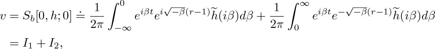
\end{align} where h(t) is compactly supported in  $(0,2)$. Using Laplace transform (see [Reference Bona, Sun and Zhang7]) or the Fokas method (see [Reference Fokas, Himonas and Mantzavinos21]), we derive the solution for the reduced pure ibvp (3.23)
 \begin{align}
v&
=
S_b[0,h;0]
\doteq
\frac{1}{2\pi}
\int_{-\infty}^0
e^{i\beta t}
e^{i\sqrt{-\beta} (r-1)}
\widetilde{h}(i\beta)d\beta
+
\frac{1}{2\pi}
\int_0^{\infty}
e^{i\beta t}
e^{-\sqrt{-\beta} (r-1)}
\widetilde{h}(i\beta)d\beta \nonumber\\&
=
I_1+I_2,
\end{align}
\begin{align}
v&
=
S_b[0,h;0]
\doteq
\frac{1}{2\pi}
\int_{-\infty}^0
e^{i\beta t}
e^{i\sqrt{-\beta} (r-1)}
\widetilde{h}(i\beta)d\beta
+
\frac{1}{2\pi}
\int_0^{\infty}
e^{i\beta t}
e^{-\sqrt{-\beta} (r-1)}
\widetilde{h}(i\beta)d\beta \nonumber\\&
=
I_1+I_2,
\end{align}where the integrals I 1 and I 2 are defined by
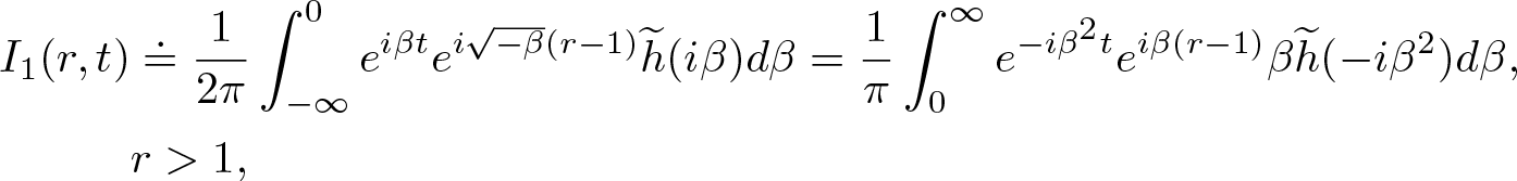 \begin{align}
I_1(r,t)
&\doteq
\frac{1}{2\pi}
\int_{-\infty}^0
e^{i\beta t}
e^{i\sqrt{-\beta} (r-1)}
\widetilde{h}(i\beta)d\beta
=
\frac{1}{\pi}
\int_{0}^\infty
e^{-i\beta^2 t}
e^{i\beta (r-1)}
\beta
\widetilde{h}(-i\beta^2)d\beta,\\ &
r \gt 1,
\end{align}
\begin{align}
I_1(r,t)
&\doteq
\frac{1}{2\pi}
\int_{-\infty}^0
e^{i\beta t}
e^{i\sqrt{-\beta} (r-1)}
\widetilde{h}(i\beta)d\beta
=
\frac{1}{\pi}
\int_{0}^\infty
e^{-i\beta^2 t}
e^{i\beta (r-1)}
\beta
\widetilde{h}(-i\beta^2)d\beta,\\ &
r \gt 1,
\end{align} \begin{align}
I_2(r,t)
\doteq &
\frac{1}{2\pi}
\int_0^{\infty}
e^{i\beta t}
e^{-\sqrt{-\beta} (r-1)}
\widetilde{h}(i\beta)d\beta
=
\frac{1}{\pi}
\int_0^{\infty}
e^{i\beta^2 t}
e^{-\beta (r-1)}
\beta
\widetilde{h}(i\beta^2)d\beta,
\quad
r \gt 1.
\end{align}
\begin{align}
I_2(r,t)
\doteq &
\frac{1}{2\pi}
\int_0^{\infty}
e^{i\beta t}
e^{-\sqrt{-\beta} (r-1)}
\widetilde{h}(i\beta)d\beta
=
\frac{1}{\pi}
\int_0^{\infty}
e^{i\beta^2 t}
e^{-\beta (r-1)}
\beta
\widetilde{h}(i\beta^2)d\beta,
\quad
r \gt 1.
\end{align} Since h(t) is compactly supported in  $(0,2)$, we have
 \begin{equation}
\widetilde{h}(-i\beta^2)
=
\int_0^\infty
e^{i\beta^2 t}
h(t)
dt
=
\int_{\mathbb R}
e^{i\beta^2 t}
h(t)
dt
=
\widehat{h}(-\beta^2)
\quad
\text{and}
\quad
\widetilde{h}(i\beta^2)
=
\widehat{h}(\beta^2).
\end{equation}
\begin{equation}
\widetilde{h}(-i\beta^2)
=
\int_0^\infty
e^{i\beta^2 t}
h(t)
dt
=
\int_{\mathbb R}
e^{i\beta^2 t}
h(t)
dt
=
\widehat{h}(-\beta^2)
\quad
\text{and}
\quad
\widetilde{h}(i\beta^2)
=
\widehat{h}(\beta^2).
\end{equation}Proposition 3.4. The solution  $v=S_b[0,h; 0]$ of the ibvp (3.20) given by formula (3.24) satisfies the space estimate:
 \begin{align}
\sup\limits_{t\in[0,T]}
\|
S_b[0, h; 0](t)
\|_{H^s(1,\infty)}
\lesssim
\|
h
\|_{H^{\frac{2s+1}{4}}({\mathbb R})},
\quad
s\ge 0.
\end{align}
\begin{align}
\sup\limits_{t\in[0,T]}
\|
S_b[0, h; 0](t)
\|_{H^s(1,\infty)}
\lesssim
\|
h
\|_{H^{\frac{2s+1}{4}}({\mathbb R})},
\quad
s\ge 0.
\end{align} Also, if  $\frac{2}{q}+\frac{1}{\gamma}=\frac12$ then $S_b[0,h; 0](r,t)$ satisfies the following Strichartz estimate
 \begin{align}
\|
S_b[0,h; 0]
\|_{L_t^q(0,T; W^{s,\gamma}(1,\infty))}
\lesssim
\|
h
\|_{H^{\frac{2s+1}{4}}({\mathbb R})},
\quad
s\ge 0.
\end{align}
\begin{align}
\|
S_b[0,h; 0]
\|_{L_t^q(0,T; W^{s,\gamma}(1,\infty))}
\lesssim
\|
h
\|_{H^{\frac{2s+1}{4}}({\mathbb R})},
\quad
s\ge 0.
\end{align}Proof of proposition 3.4
For the proof of estimate (3.28), we refer to [Reference Bona, Sun and Zhang7, Reference Fokas, Himonas and Mantzavinos21]. Here, we only provide the proof of Strichartz estimate (3.29), which was also discussed in [Reference Bona, Sun and Zhang7]. In this exposition, we offer an alternative proof.
Proof of Strichartz estimate (3.29). The proof for I 1 is similar to that of estimate (3.14) and here we omit it. Next, we prove estimate (3.29) for I 2. Making the change of variables  $\tau=\beta^2$, we get
 \begin{align}
I_{2}(r,t)
\simeq
\int_0^{\infty}
e^{i\tau t}
e^{-\sqrt{\tau} (r-1)}
\widehat{h}(\tau)d\tau
=
\int_0^{\infty}
K_t(r,\tau)
\cdot
(1+|\tau|)^{\frac14}
\widehat{h}(\tau)d\tau
,
\quad
r \gt 1,
\end{align}
\begin{align}
I_{2}(r,t)
\simeq
\int_0^{\infty}
e^{i\tau t}
e^{-\sqrt{\tau} (r-1)}
\widehat{h}(\tau)d\tau
=
\int_0^{\infty}
K_t(r,\tau)
\cdot
(1+|\tau|)^{\frac14}
\widehat{h}(\tau)d\tau
,
\quad
r \gt 1,
\end{align} where the kernel  $K_t(r,\tau)$ is defined as follows
 \begin{equation}
K_t(r,\tau)
\doteq
e^{i\tau t}
e^{-\sqrt{\tau} (r-1)}
(1+|\tau|)^{-\frac14},
\quad
r \gt 1.
\end{equation}
\begin{equation}
K_t(r,\tau)
\doteq
e^{i\tau t}
e^{-\sqrt{\tau} (r-1)}
(1+|\tau|)^{-\frac14},
\quad
r \gt 1.
\end{equation}Also, we see that estimate (3.29) follows from the following result
 \begin{equation}
\Big\|
\int_0^\infty
K_t(r,\tau)
\widehat{f}(\tau)
d\tau
\Big\|_{L_t^q(0,T; L^{\gamma}(1,\infty))}
\lesssim
\|f\|_{L^2},
\quad
\frac{2}{q}+\frac{1}{\gamma}=\frac12
\,\,
\text{and}
\,\,
2\le \gamma\le \infty.
\end{equation}
\begin{equation}
\Big\|
\int_0^\infty
K_t(r,\tau)
\widehat{f}(\tau)
d\tau
\Big\|_{L_t^q(0,T; L^{\gamma}(1,\infty))}
\lesssim
\|f\|_{L^2},
\quad
\frac{2}{q}+\frac{1}{\gamma}=\frac12
\,\,
\text{and}
\,\,
2\le \gamma\le \infty.
\end{equation}The proof of estimate (3.32) is provided in Appendix. Now, using (3.32), we show the estimate (3.29). To do this, we will consider the following two cases.
Case 1:  $s\in {\mathbb{N}}$. Taking partial derivative $\partial_r^s$, we have
 \begin{align}
\partial_r^s I_{2}(r,t)
\simeq
\int_0^{\infty}
e^{i\tau t}
e^{-\sqrt{\tau} (r-1)}
(-\sqrt{\tau})^s
\widehat{h}(\tau)d\tau
\simeq
\int_0^{\infty}
K_t(r,\tau)
\cdot
|\tau|^{\frac{s}{2}}
(1+|\tau|)^{\frac14}
\widehat{h}(\tau)d\tau.
\end{align}
\begin{align}
\partial_r^s I_{2}(r,t)
\simeq
\int_0^{\infty}
e^{i\tau t}
e^{-\sqrt{\tau} (r-1)}
(-\sqrt{\tau})^s
\widehat{h}(\tau)d\tau
\simeq
\int_0^{\infty}
K_t(r,\tau)
\cdot
|\tau|^{\frac{s}{2}}
(1+|\tau|)^{\frac14}
\widehat{h}(\tau)d\tau.
\end{align} Next, apply (3.32) with  $\widehat{f}(\tau)=|\tau|^{\frac{s}{2}}
(1+|\tau|)^{\frac14}
\widehat{h}(\tau)$ to obtain
$\widehat{f}(\tau)=|\tau|^{\frac{s}{2}}
(1+|\tau|)^{\frac14}
\widehat{h}(\tau)$ to obtain
 \begin{align*}
\Big\|
I_{2}
\Big\|_{L_t^q(0,T; W^{s,\gamma}(1,\infty))}&
=
\Big\|
\partial_r^sI_{2}
\Big\|_{L_t^q(0,T; L^{\gamma}(1,\infty))}
\lesssim
\Big(
\int_{\mathbb R}
|\tau|^{s}
(1+|\tau|)^{\frac12}
|\widehat{h}(\tau)|^2
d\tau
\Big)^{1/2}\\&
\lesssim
\|h\|_{H^{\frac{2s+1}{4}}},
\end{align*}
\begin{align*}
\Big\|
I_{2}
\Big\|_{L_t^q(0,T; W^{s,\gamma}(1,\infty))}&
=
\Big\|
\partial_r^sI_{2}
\Big\|_{L_t^q(0,T; L^{\gamma}(1,\infty))}
\lesssim
\Big(
\int_{\mathbb R}
|\tau|^{s}
(1+|\tau|)^{\frac12}
|\widehat{h}(\tau)|^2
d\tau
\Big)^{1/2}\\&
\lesssim
\|h\|_{H^{\frac{2s+1}{4}}},
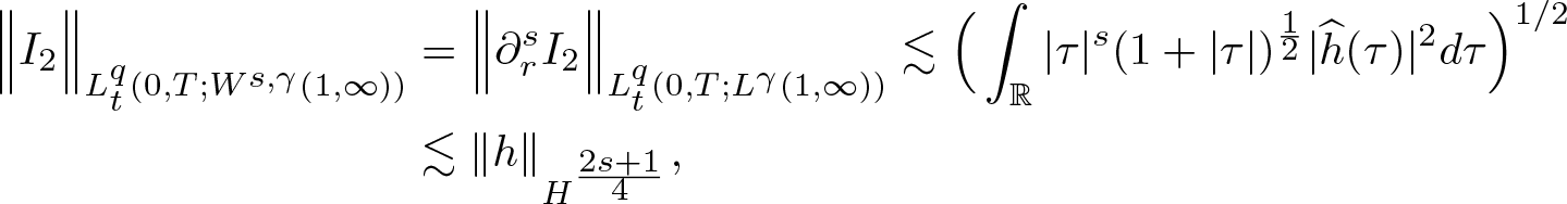
\end{align*}which is the desired estimate (3.29).
Case 2:  $s\ge 0$ and $s\not\in {\mathbb{N}}$. We prove this by interpolation. In fact, any $s\ge 0$ can be written as
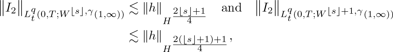
  $s=(1-\theta)\lfloor s\rfloor+\theta(\lfloor s\rfloor+1)$. Furthermore, in Case 1, we proved that
 \begin{align*}
\big\|
I_{2}
\big\|_{L_t^q(0,T; W^{\lfloor s\rfloor,\gamma}(1,\infty))}&
\lesssim
\|h\|_{H^{\frac{2\lfloor s\rfloor+1}{4}}}
\quad
\text{and}
\quad
\big\|
I_{2}
\big\|_{L_t^q(0,T; W^{\lfloor s\rfloor+1,\gamma}(1,\infty))}\\&
\lesssim
\|h\|_{H^{\frac{2(\lfloor s\rfloor+1)+1}{4}}},
\end{align*}
\begin{align*}
\big\|
I_{2}
\big\|_{L_t^q(0,T; W^{\lfloor s\rfloor,\gamma}(1,\infty))}&
\lesssim
\|h\|_{H^{\frac{2\lfloor s\rfloor+1}{4}}}
\quad
\text{and}
\quad
\big\|
I_{2}
\big\|_{L_t^q(0,T; W^{\lfloor s\rfloor+1,\gamma}(1,\infty))}\\&
\lesssim
\|h\|_{H^{\frac{2(\lfloor s\rfloor+1)+1}{4}}},
\end{align*} which implies that I 2 is a continuous linear operator from  $H^{\frac{2\lfloor s\rfloor+1}{4}}$ to $L_t^q(0,T; W^{\lfloor s\rfloor,\gamma}(1,\infty))$ as well as from $H^{\frac{2(\lfloor s\rfloor+1)+1}{4}}$ to $L_t^q(0,T; W^{\lfloor s\rfloor+1,\gamma}(1,\infty))$. Thus, according to Theorem 5.1 of [Reference Lions and Magenes30] (see also [Reference Bergh and Löfström3]), we see that I 2 is a continuous linear operator from $H^{\frac{2s+1}{4}}$ to $L_t^q(0,T; W^{s,\gamma}(1,\infty))$. This completes the proof of Case 2 and estimate (3.29).
Now, we can derive the linear estimate for the solution of ibvp (3.1). In fact, this solution is given by
 \begin{align}
v(r,t)&
=
\Lambda[v_0, g; f_1]
\doteq
S[V_0;0]
+
S[0; F]
+
S_b[0, g-S[V_0;F](1,t);0 ],
\quad
r \gt 1,\\ &
t\in(0,T),
\end{align}
\begin{align}
v(r,t)&
=
\Lambda[v_0, g; f_1]
\doteq
S[V_0;0]
+
S[0; F]
+
S_b[0, g-S[V_0;F](1,t);0 ],
\quad
r \gt 1,\\ &
t\in(0,T),
\end{align}where V 0 is an extension of v 0 satisfying inequality (3.6) and F is an extension of f 1 satisfying inequality (3.9). Combining propositions 3.1–3.4 and using inequalities (3.6) and (3.9), we obtain the following linear estimate.
Theorem 3.5 The following estimates hold.
(1) Suppose that
$0\le s \lt \frac12$. If $v_0\in H^s(1,\infty)$, $g\in H^{\frac{2s+1}{4}}(0,T)$ and $f_1\in L_t^{q'}\big(0,T;$ $W^{s,\gamma'}(1,\infty)\big)$, where $(q,\gamma)$ is admissible with n = 1, then $\Lambda[v_0, g; f_1]$ defines a solution to the linear ibvp (3.1), which satisfies
(3.35)\begin{align}
&\sup\limits_{t\in[0,T]}\big\|\Lambda[v_0, g; f_1](t)\big\|_{H^s(1,\infty)}
+
\big\|\Lambda[v_0, g; f_1]\big\|_{L_t^{q}(0,T; W^{s,\gamma}(1,\infty))}
\nonumber
\\
& \qquad \lesssim
\|v_0\|_{H^s(1,\infty)}
+
\|g\|_{H^{\frac{2s+1}{4}}(0,T)}
+
\|f_1\|_{L_t^{q'}(0,T; W^{s,\gamma'}(1,\infty))}.
\end{align}(2) Suppose that
$\frac12 \lt s \lt \frac32$. If $v_0\in H^s(1,\infty)$, $g\in H^{\frac{2s+1}{4}}(0,T)$ and $f_1\in L^1\big(0,T; H^s(1,\infty)\big)$ then $\Lambda[v_0, g; f_1]$ defines a solution to the linear ibvp (3.1) with compatibility condition (3.2), which satisfies
(3.36)\begin{align}
\sup\limits_{t\in[0,T]}\big\|\Lambda[v_0, g; f_1](t)\big\|_{H^s(1,\infty)}
\lesssim&
\|v_0\|_{H^s(1,\infty)}
+
\|g\|_{H^{\frac{2s+1}{4}}(0,T)}\nonumber\\&
+
\big\|f_1\big\|_{L^1\big(0,T; H^s(1,\infty)\big)}.
\end{align}


3.2. Proof of well-posedness for ibvp in domain Ω1, i.e., theorem 1.2
Existence of solutions for nonlinear problems on half line. Since the ibvp in Ω1 is reduced to the ibvp (2.1) for  $r \in ( 1, \infty)$ with $u (1, t ) = g(t)$. Now, it suffices to prove the existence of solutions of ibvp (3.1) with forcing f 1 giving by
 \begin{align}
f_1(r,t)&
=
-\lambda r^{\frac{n-1}2}|u|^{p-2}u+\frac{n^2-4n+3}{4}r^{-2}\cdot v
=
-\lambda r^{-\frac{(n-1)(p-2)}2}|v|^{p-2}v \nonumber\\& +\frac{n^2-4n+3}{4}r^{-2}\cdot v.
\end{align}
\begin{align}
f_1(r,t)&
=
-\lambda r^{\frac{n-1}2}|u|^{p-2}u+\frac{n^2-4n+3}{4}r^{-2}\cdot v
=
-\lambda r^{-\frac{(n-1)(p-2)}2}|v|^{p-2}v \nonumber\\& +\frac{n^2-4n+3}{4}r^{-2}\cdot v.
\end{align} The case.  $0\le s \lt \frac12$.. In the solution formula (3.34), replacing f 1 by the nonlinearity above, we obtain the iteration map
 \begin{equation}
v
=
\Lambda\big[v_0, g; f_1]
=
\Lambda\big[v_0, g;
-\lambda r^{-\frac{(n-1)(p-2)}2}|v|^{p-2}v+\frac{n^2-4n+3}{4}r^{-2}\cdot v
\big].
\end{equation}
\begin{equation}
v
=
\Lambda\big[v_0, g; f_1]
=
\Lambda\big[v_0, g;
-\lambda r^{-\frac{(n-1)(p-2)}2}|v|^{p-2}v+\frac{n^2-4n+3}{4}r^{-2}\cdot v
\big].
\end{equation}Next, we will show that the iteration map (3.38) is a contraction in the following solution space
 \begin{equation}
Z
=
C([0,T^*]; H^s(1,\infty))
\cap
L_t^{q}(0,T^*; W^{s,\gamma}(1,\infty)),
\end{equation}
\begin{equation}
Z
=
C([0,T^*]; H^s(1,\infty))
\cap
L_t^{q}(0,T^*; W^{s,\gamma}(1,\infty)),
\end{equation} where  $(q,\gamma)$ is an admissible pair (with n = 1), which are defined as
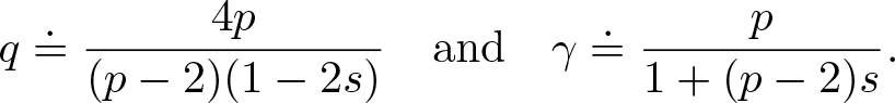 \begin{equation}q\doteq\frac{4p}{(p-2)(1-2s)}\quad\text{and}\quad\gamma\doteq\frac p{1+(p-2)s}.\end{equation}
 We notice that q and γ satisfy  $\gamma\ge2$ and $q\ge 2\big(\frac{2}{1-2s}+1\big)$. The linear estimate (3.35) implies
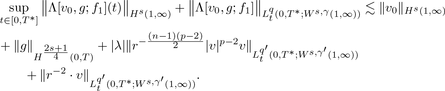 \begin{align}
&\sup\limits_{t\in[0,T^*]}\big\|\Lambda[v_0, g; f_1](t)\big\|_{H^s(1,\infty)}
+
\big\|\Lambda[v_0, g; f_1]\big\|_{L_t^{q}(0,T^*; W^{s,\gamma}(1,\infty))}
\lesssim
\|v_0\|_{H^s(1,\infty)} \nonumber \\ \quad
&
+
\|g\|_{H^{\frac{2s+1}{4}}(0,T)} +
|\lambda|
\|r^{-\frac{(n-1)(p-2)}2}|v|^{p-2}v\|_{L_t^{q'}(0,T^*; W^{s,\gamma'}(1,\infty))} \nonumber \\
&\qquad
+
\|r^{-2}\cdot v\|_{L_t^{q'}(0,T^*; W^{s,\gamma'}(1,\infty))}.
\end{align}
\begin{align}
&\sup\limits_{t\in[0,T^*]}\big\|\Lambda[v_0, g; f_1](t)\big\|_{H^s(1,\infty)}
+
\big\|\Lambda[v_0, g; f_1]\big\|_{L_t^{q}(0,T^*; W^{s,\gamma}(1,\infty))}
\lesssim
\|v_0\|_{H^s(1,\infty)} \nonumber \\ \quad
&
+
\|g\|_{H^{\frac{2s+1}{4}}(0,T)} +
|\lambda|
\|r^{-\frac{(n-1)(p-2)}2}|v|^{p-2}v\|_{L_t^{q'}(0,T^*; W^{s,\gamma'}(1,\infty))} \nonumber \\
&\qquad
+
\|r^{-2}\cdot v\|_{L_t^{q'}(0,T^*; W^{s,\gamma'}(1,\infty))}.
\end{align}Now, we need to bound the nonlinear terms in the above inequality.
Estimate for.  $\|r^{-\frac{(n-1)(p-2)}2}|v|^{p-2}v\|_{L_t^{q'}(0,T^*; W^{s,\gamma'}(1,\infty))}$. We extend $r^{-\frac{(n-1)(p-2)}2}$ from $(1,\infty)$ to ${\mathbb R}$ such that the extension $k(r)\in C^\infty({\mathbb R})$ and it is described as follows
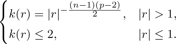 \begin{align*}
\begin{cases}
k(r)
=
|r|^{-\frac{(n-1)(p-2)}2},
\quad
&|r| \gt 1,
\\
k(r)\le 2,
\quad
&|r|\le1.
\end{cases}
\end{align*}
\begin{align*}
\begin{cases}
k(r)
=
|r|^{-\frac{(n-1)(p-2)}2},
\quad
&|r| \gt 1,
\\
k(r)\le 2,
\quad
&|r|\le1.
\end{cases}
\end{align*} Also, we extend v from  $(1,\infty)\times(0,T^*)$ to ${\mathbb R}\times (0,T^*)$ such that the extension V satisfies
 \begin{equation}
\|V\|_{L_t^{q}(0,T^*; W^{s,\gamma}({\mathbb R}))}
\le
2
\|v\|_{L_t^{q}(0,T^*; W^{s,\gamma}(1,\infty))}.
\end{equation}
\begin{equation}
\|V\|_{L_t^{q}(0,T^*; W^{s,\gamma}({\mathbb R}))}
\le
2
\|v\|_{L_t^{q}(0,T^*; W^{s,\gamma}(1,\infty))}.
\end{equation}Now, we have
 \begin{align*}
\|r^{-\frac{(n-1)(p-2)}2}|v|^{p-2}v\|_{L_t^{q'}(0,T^*; W^{s,\gamma'}(1,\infty))}
\le
\|k(\cdot)|V|^{p-2}V\|_{L_t^{q'}(0,T^*; W^{s,\gamma'}({\mathbb R}))}.
\end{align*}
\begin{align*}
\|r^{-\frac{(n-1)(p-2)}2}|v|^{p-2}v\|_{L_t^{q'}(0,T^*; W^{s,\gamma'}(1,\infty))}
\le
\|k(\cdot)|V|^{p-2}V\|_{L_t^{q'}(0,T^*; W^{s,\gamma'}({\mathbb R}))}.
\end{align*} Furthermore, using the chain rule (see lemma 5 in [Reference Holmer25]) and using  $\|k\|_{L^\infty}\le 2$, we obtain
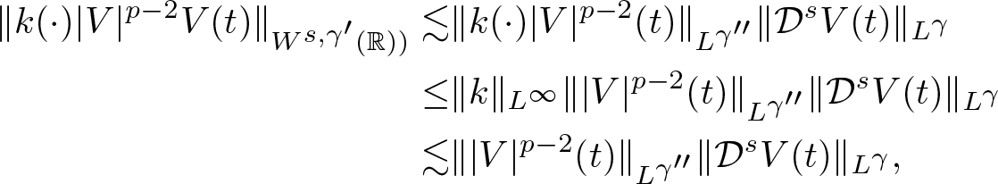 \begin{align*}
\|k(\cdot)|V|^{p-2}V(t)\|_{W^{s,\gamma'}({\mathbb R}))}
\lesssim&
\|k(\cdot)|V|^{p-2}(t)\|_{L^{\gamma''}}
\|\mathcal{D}^sV(t)\|_{L^{\gamma}}
\\
\le&
\|k\|_{L^\infty}
\||V|^{p-2}(t)\|_{L^{\gamma''}}
\|\mathcal{D}^sV(t)\|_{L^{\gamma}}\\
\lesssim&
\||V|^{p-2}(t)\|_{L^{\gamma''}}
\|\mathcal{D}^sV(t)\|_{L^{\gamma}},
\end{align*}
\begin{align*}
\|k(\cdot)|V|^{p-2}V(t)\|_{W^{s,\gamma'}({\mathbb R}))}
\lesssim&
\|k(\cdot)|V|^{p-2}(t)\|_{L^{\gamma''}}
\|\mathcal{D}^sV(t)\|_{L^{\gamma}}
\\
\le&
\|k\|_{L^\infty}
\||V|^{p-2}(t)\|_{L^{\gamma''}}
\|\mathcal{D}^sV(t)\|_{L^{\gamma}}\\
\lesssim&
\||V|^{p-2}(t)\|_{L^{\gamma''}}
\|\mathcal{D}^sV(t)\|_{L^{\gamma}},
\end{align*} where  $\frac{1}{\gamma''}=\frac{1}{\gamma'}-\frac1\gamma=1-\frac{2}{\gamma}$. Moreover, applying Sobolev–Gagliardo–Nirenberg inequality (we refer to theorem 1.3.4 in [Reference Cazenave and Haraux12] and corollary 1.5 in [Reference Hajaiej, Molinet, Ozawa, Wang, Ozawa and Sugimoto23]) with $\frac{1}{(p-2)\gamma''}=\frac{1}{\gamma}-s$, it is obtained that
  $ \||V|^{p-2}(t)\|_{L^{\gamma''}}\lesssim
\|\mathcal{D}^sV(t)\|_{L^{\gamma}}^{p-2}$. Finally, combining above inequalities with Hölder’s inequality and using inequality (3.42) give
$ \||V|^{p-2}(t)\|_{L^{\gamma''}}\lesssim
\|\mathcal{D}^sV(t)\|_{L^{\gamma}}^{p-2}$. Finally, combining above inequalities with Hölder’s inequality and using inequality (3.42) give
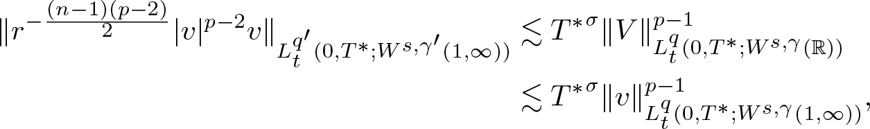 \begin{align}
\|r^{-\frac{(n-1)(p-2)}2}|v|^{p-2}v\|_{L_t^{q'}(0,T^*; W^{s,\gamma'}(1,\infty))}&
\lesssim
{T^*}^\sigma
\|V\|_{L_t^{q}(0,T^*; W^{s,\gamma}({\mathbb R}))}^{p-1}\\&
\lesssim
{T^*}^\sigma
\|v\|_{L_t^{q}(0,T^*; W^{s,\gamma}(1,\infty))}^{p-1},
\end{align}
\begin{align}
\|r^{-\frac{(n-1)(p-2)}2}|v|^{p-2}v\|_{L_t^{q'}(0,T^*; W^{s,\gamma'}(1,\infty))}&
\lesssim
{T^*}^\sigma
\|V\|_{L_t^{q}(0,T^*; W^{s,\gamma}({\mathbb R}))}^{p-1}\\&
\lesssim
{T^*}^\sigma
\|v\|_{L_t^{q}(0,T^*; W^{s,\gamma}(1,\infty))}^{p-1},
\end{align}for some σ > 0. Working similarly to inequality (3.43) (see also [Reference Holmer25, Reference Himonas and Mantzavinos27]), we have
 \begin{align}
&\|r^{-\frac{(n-1)(p-2)}2}(|v_1|^{p-2}v_1-|v_2|^{p-2}v_2)\|_{L_t^{q'}(0,T^*; W^{s,\gamma'}(1,\infty))}
\nonumber
\\
\lesssim&
{T^*}^\sigma
(\|v_1\|_{L_t^{q}(0,T^*; W^{s,\gamma}(1,\infty))}^{p-2}+\|v_2\|_{L_t^{q}(0,T^*; W^{s,\gamma}(1,\infty))}^{p-2})
\|v_1-v_2\|_{L_t^{q}(0,T^*; W^{s,\gamma}(1,\infty))} \, .
\end{align}
\begin{align}
&\|r^{-\frac{(n-1)(p-2)}2}(|v_1|^{p-2}v_1-|v_2|^{p-2}v_2)\|_{L_t^{q'}(0,T^*; W^{s,\gamma'}(1,\infty))}
\nonumber
\\
\lesssim&
{T^*}^\sigma
(\|v_1\|_{L_t^{q}(0,T^*; W^{s,\gamma}(1,\infty))}^{p-2}+\|v_2\|_{L_t^{q}(0,T^*; W^{s,\gamma}(1,\infty))}^{p-2})
\|v_1-v_2\|_{L_t^{q}(0,T^*; W^{s,\gamma}(1,\infty))} \, .
\end{align} Estimate for  $\|r^{-2}v\|_{L_t^{q'}(0,T^*; W^{s,\gamma'}(1,\infty))}$. Since $r^{-2}\in C^\infty(1,\infty)$ and it is bounded by 1, we derive
 \begin{align}
&\|r^{-2}v\|_{L_t^{q'}(0,T^*; W^{s,\gamma'}(1,\infty))}
\lesssim
{T^*}^\sigma
\|v\|_{L_t^{q}(0,T^*; W^{s,\gamma}(1,\infty))},
\end{align}
\begin{align}
&\|r^{-2}v\|_{L_t^{q'}(0,T^*; W^{s,\gamma'}(1,\infty))}
\lesssim
{T^*}^\sigma
\|v\|_{L_t^{q}(0,T^*; W^{s,\gamma}(1,\infty))},
\end{align} \begin{align}
&\|r^{-2}(v_1-v_2)\|_{L_t^{q'}(0,T^*; W^{s,\gamma'}(1,\infty))}
\lesssim
{T^*}^\sigma
\|v_1-v_2\|_{L_t^{q}(0,T^*; W^{s,\gamma}(1,\infty))}.
\end{align}
\begin{align}
&\|r^{-2}(v_1-v_2)\|_{L_t^{q'}(0,T^*; W^{s,\gamma'}(1,\infty))}
\lesssim
{T^*}^\sigma
\|v_1-v_2\|_{L_t^{q}(0,T^*; W^{s,\gamma}(1,\infty))}.
\end{align} Combining linear estimate (3.41) with inequalities (3.44) and (3.45), we can show that the iteration map (3.38) is contraction in solution space Z for small  $T^*$. Since the argument is standard, we omit it here. This completes the proof for the case $0\le s \lt \frac12$.
The case  $\frac12 \lt s \lt \frac32$. In this case, we choose $q=\infty$ and γ = 2. Since the argument is similar to the case $0\le s \lt \frac12$, the proof is omitted here.
Uniqueness and Lipschitz continuity of data-to-solution map. The argument for uniqueness and Lipschitz continuity of data-to-solution map is similar to that in [Reference Holmer25] and hence is omitted here. We complete the proof of theorem 1.2.
4. ibvp on annulus
In this section, we study the ibvp on annulus, that is, Eq. (2.1) with  $0 \lt r_1 \lt r_2 \lt + \infty $. The boundary conditions are
 \begin{equation*}
v ( r_1 , t ) =\widetilde{g}_1(t)=r_1^{\frac{n-1}{2}}g_1(t) \, , \qquad v ( r_2 , t ) = \widetilde{g}_2(t)= r_2^{\frac{n-1}{2}}g_2(t)\, .
\end{equation*}
\begin{equation*}
v ( r_1 , t ) =\widetilde{g}_1(t)=r_1^{\frac{n-1}{2}}g_1(t) \, , \qquad v ( r_2 , t ) = \widetilde{g}_2(t)= r_2^{\frac{n-1}{2}}g_2(t)\, .
\end{equation*} For the sake of convenience, we choose  $r_1=\pi$ and $r_2=2\pi$.
4.1. Linear problem on the annulus
We first consider the linear Schrödinger equation on the interval, i.e.,
 \begin{align}
&iv_t+v_{rr}=f_1(r,t),
& &
\pi \lt r \lt 2\pi,
\,\,
t\in(0,T),
\end{align}
\begin{align}
&iv_t+v_{rr}=f_1(r,t),
& &
\pi \lt r \lt 2\pi,
\,\,
t\in(0,T),
\end{align} \begin{align}
&v(r,0)
=
v_0(r),
& &
\pi \lt r \lt 2\pi,
\end{align}
\begin{align}
&v(r,0)
=
v_0(r),
& &
\pi \lt r \lt 2\pi,
\end{align} \begin{align}
&v(\pi,t)
=
\widetilde{g}_1(t),
\qquad
v(2\pi,t)
=
\widetilde{g}_2(t),
&
&
t\in(0,T),
\end{align}
\begin{align}
&v(\pi,t)
=
\widetilde{g}_1(t),
\qquad
v(2\pi,t)
=
\widetilde{g}_2(t),
&
&
t\in(0,T),
\end{align} where  $f_1(r,t)\doteq r^{\frac{n-1}2}f(r,t)+\frac{n^2-4n+3}{4}r^{-2}\cdot v$. Also, by letting $w(r,t)=v(r+\pi,t)$ and $f_2(r,t)=f_1(r+\pi,t)$, we change the problem (4.1) to the interval $(0,\pi)$. In fact, the ibvp for w is
 \begin{align}
&iw_t+w_{rr}=f_2(r,t),
& &
0 \lt r \lt \pi,
\,\,
t\in(0,T),
\end{align}
\begin{align}
&iw_t+w_{rr}=f_2(r,t),
& &
0 \lt r \lt \pi,
\,\,
t\in(0,T),
\end{align} \begin{align}
&w(r,0)
=
w_0(r)
\in H^s(0,\pi),
& &
0 \lt r \lt \pi,
\end{align}
\begin{align}
&w(r,0)
=
w_0(r)
\in H^s(0,\pi),
& &
0 \lt r \lt \pi,
\end{align} \begin{align}
&w(0,t)
=
\widetilde{g}_1(t)\in H^{\frac{s+1}{2}}(0,T),
\qquad
w(\pi,t)
=
\widetilde{g}_2(t)
\in H^{\frac{s+1}{2}}(0,T),
&
&
t\in(0,T).
\end{align}
\begin{align}
&w(0,t)
=
\widetilde{g}_1(t)\in H^{\frac{s+1}{2}}(0,T),
\qquad
w(\pi,t)
=
\widetilde{g}_2(t)
\in H^{\frac{s+1}{2}}(0,T),
&
&
t\in(0,T).
\end{align}Also, from the compatibility condition (1.8c), we have the following compatibility conditions
 \begin{equation}
\widetilde{g}_1(0)
=
w_0(0)
\quad
\text{and}
\quad
\widetilde{g}_2(0)
=
w_0(\pi),
\quad
\frac12 \lt s \lt 2.
\end{equation}
\begin{equation}
\widetilde{g}_1(0)
=
w_0(0)
\quad
\text{and}
\quad
\widetilde{g}_2(0)
=
w_0(\pi),
\quad
\frac12 \lt s \lt 2.
\end{equation} Using this, for  $\frac12 \lt s \lt 2$, we can assume that $w_0(0)=w_0(\pi)=\widetilde{g}_1(0)=\widetilde{g}_2(0)=0$.
Next, we solve the ibvp (4.2) by decomposing it into simpler problems. In fact, using superposition principle, the linear ibvp (4.2) can be expressed as the homogeneous ibvp
 \begin{align}
&iw_t+w_{rr}
=
0,
& &
0 \lt r \lt \pi,
\,\,t\in(0,T),
\end{align}
\begin{align}
&iw_t+w_{rr}
=
0,
& &
0 \lt r \lt \pi,
\,\,t\in(0,T),
\end{align} \begin{align}
&w(r,0)
=
w_0(r),
& &
0 \lt r \lt \pi,
\end{align}
\begin{align}
&w(r,0)
=
w_0(r),
& &
0 \lt r \lt \pi,
\end{align} \begin{align}
&w(0,t)
=
\widetilde{g}_1(t),
\qquad
w(\pi,t)
=
\widetilde{g}_2(t),
&
&
t\in(0,T),
\end{align}
\begin{align}
&w(0,t)
=
\widetilde{g}_1(t),
\qquad
w(\pi,t)
=
\widetilde{g}_2(t),
&
&
t\in(0,T),
\end{align}and the forced linear ibvp with zero initial and boundary data
 \begin{align}
&iw_t+w_{rr}
=
f_2(r,t),
& &0 \lt r \lt \pi,\,\,t\in(0,T),
\end{align}
\begin{align}
&iw_t+w_{rr}
=
f_2(r,t),
& &0 \lt r \lt \pi,\,\,t\in(0,T),
\end{align} \begin{align}
&w(r,0)
=
0,
& &0 \lt r \lt \pi,
\end{align}
\begin{align}
&w(r,0)
=
0,
& &0 \lt r \lt \pi,
\end{align} \begin{align}
&w(0,t)
=
0,
\qquad
w(\pi,t)
=
0,
&
&
t\in(0,T).
\end{align}
\begin{align}
&w(0,t)
=
0,
\qquad
w(\pi,t)
=
0,
&
&
t\in(0,T).
\end{align}In addition, we decompose the ibvp (4.4) as an ibvp with homogeneous boundary data
 \begin{align}
&iv_t+v_{rr}
=
0,
& &
0 \lt r \lt \pi,
\,\,t\in(0,T),
\end{align}
\begin{align}
&iv_t+v_{rr}
=
0,
& &
0 \lt r \lt \pi,
\,\,t\in(0,T),
\end{align} \begin{align}
&v(r,0)
=
\omega_0(r),
& &
0 \lt r \lt \pi,
\end{align}
\begin{align}
&v(r,0)
=
\omega_0(r),
& &
0 \lt r \lt \pi,
\end{align} \begin{align}
&v(0,t)
=
0,
\qquad
v(\pi,t)
=
0,
&
&
t\in(0,T),
\end{align}
\begin{align}
&v(0,t)
=
0,
\qquad
v(\pi,t)
=
0,
&
&
t\in(0,T),
\end{align}and an ibvp with zero initial data:
 \begin{align}
&iw_t+w_{rr}
=
0,
& &
0 \lt r \lt \pi,
\,\,t\in(0,T),
\end{align}
\begin{align}
&iw_t+w_{rr}
=
0,
& &
0 \lt r \lt \pi,
\,\,t\in(0,T),
\end{align} \begin{align}
&w(r,0)
=
0,
& &
0 \lt r \lt \pi,
\end{align}
\begin{align}
&w(r,0)
=
0,
& &
0 \lt r \lt \pi,
\end{align} \begin{align}
&w(0,t)
=
h_1(t),
\quad
w(\pi,t)
=
h_2(t),
&&
t\in(0,T),
\end{align}
\begin{align}
&w(0,t)
=
h_1(t),
\quad
w(\pi,t)
=
h_2(t),
&&
t\in(0,T),
\end{align} where  $h_1=\widetilde{g}_1(t)$ and $h_2=\widetilde{g}_2(t)$.
Solving the ibvp (4.6). We will solve this problem by reflection. In fact, in order to solve this problem, it suffices to solve the following periodic problem
 \begin{align}
&iV_t+V_{rr}
=
0,
& &
-\pi \lt r \lt \pi,
\,\,t\in(0,T),
\end{align}
\begin{align}
&iV_t+V_{rr}
=
0,
& &
-\pi \lt r \lt \pi,
\,\,t\in(0,T),
\end{align} \begin{align}
&V(r,0)
=
V_0(r),
& &
-\pi \lt r \lt \pi,
\end{align}
\begin{align}
&V(r,0)
=
V_0(r),
& &
-\pi \lt r \lt \pi,
\end{align} \begin{align}
&V(-\pi,t)
=
V(\pi,t),
\quad
V_r(-\pi,t)
=
V_r(\pi,t),
&
&
t\in(0,T),
\end{align}
\begin{align}
&V(-\pi,t)
=
V(\pi,t),
\quad
V_r(-\pi,t)
=
V_r(\pi,t),
&
&
t\in(0,T),
\end{align} where  $V_0(r)$ is the odd extension of $w_0(r)$, i.e.,
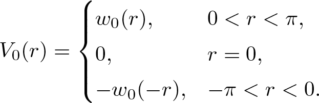 \begin{align}
V_0(r)
=
\begin{cases}
w_0(r),
\quad
&0 \lt r \lt \pi,
\\
0,
\quad
&r=0,
\\
-w_0(-r),
\quad
&
-\pi \lt r \lt 0.
\end{cases}
\end{align}
\begin{align}
V_0(r)
=
\begin{cases}
w_0(r),
\quad
&0 \lt r \lt \pi,
\\
0,
\quad
&r=0,
\\
-w_0(-r),
\quad
&
-\pi \lt r \lt 0.
\end{cases}
\end{align}By using the standard separation of variables, the solution to the periodic ivp (4.8) is
 \begin{equation}
V
=
W_0(t)w_0
\doteq
\sum\limits_{n=1}^\infty
B_n \sin (n r)
e^{-i n^2 t },
\end{equation}
\begin{equation}
V
=
W_0(t)w_0
\doteq
\sum\limits_{n=1}^\infty
B_n \sin (n r)
e^{-i n^2 t },
\end{equation}where
 \begin{equation}
B_n
=
\frac{2}{\pi}\int_0^\pi
w_0(r)
\sin (n r)
dr,
\quad
n\in {\mathbb Z}.
\end{equation}
\begin{equation}
B_n
=
\frac{2}{\pi}\int_0^\pi
w_0(r)
\sin (n r)
dr,
\quad
n\in {\mathbb Z}.
\end{equation} The solution formula  $ W_0(t)w_0$ can also be written in the complex form
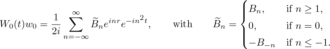 \begin{equation}
W_0(t)w_0
=
\frac1{2i}
\sum\limits_{n=-\infty}^\infty
\widetilde{B}_n e^{in r}
e^{-i n^2 t },
\qquad
\text{with}
\qquad
\widetilde{B}_n
=
\begin{cases}
B_n,
\quad
&
\text{if}\,\,
n\ge 1,
\\
0,
\quad
&
\text{if}\,\,
n=0,
\\
-B_{-n}
\quad
&
\text{if}\,\,
n\le -1.
\end{cases}
\end{equation}
\begin{equation}
W_0(t)w_0
=
\frac1{2i}
\sum\limits_{n=-\infty}^\infty
\widetilde{B}_n e^{in r}
e^{-i n^2 t },
\qquad
\text{with}
\qquad
\widetilde{B}_n
=
\begin{cases}
B_n,
\quad
&
\text{if}\,\,
n\ge 1,
\\
0,
\quad
&
\text{if}\,\,
n=0,
\\
-B_{-n}
\quad
&
\text{if}\,\,
n\le -1.
\end{cases}
\end{equation} Furthermore, for w 0, we define  $H^{s}(0,\pi)$-norm by its Fourier coefficients as follows
 \begin{equation}
\|w_0\|_{H^s(0,\pi)}^2
\doteq
\sum\limits_{n=1}^\infty
(1+n)^{2s}
b_n^2,
\end{equation}
\begin{equation}
\|w_0\|_{H^s(0,\pi)}^2
\doteq
\sum\limits_{n=1}^\infty
(1+n)^{2s}
b_n^2,
\end{equation} where the Fourier coefficient  $b_n=B_n$ is defined as follows
 \begin{equation}
b_n
\doteq
\frac{2}{\pi}
\int_0^\pi
w_0(r)
\sin (nr)
dr
=
B_n,
\quad
n\ge 1.
\end{equation}
\begin{equation}
b_n
\doteq
\frac{2}{\pi}
\int_0^\pi
w_0(r)
\sin (nr)
dr
=
B_n,
\quad
n\ge 1.
\end{equation} Finally, we state the following result for the solution  $ W_0(t)w_0$ given by (4.10).
Proposition 4.1. Let  $w_0\in H^s(0,\pi)$, where $0\le s\le 2$ and $s\neq\frac12,\frac32$. Then, the solution defined by (4.10) satisfies the following estimates
 \begin{align}
\sup\limits_{t\in[0,T]}\|W_0(t)w_0\|_{H^{s}(0,\pi)}
\le C_{T,s}
\|w_0 \|_{H^s(0,\pi)}.
\end{align}
\begin{align}
\sup\limits_{t\in[0,T]}\|W_0(t)w_0\|_{H^{s}(0,\pi)}
\le C_{T,s}
\|w_0 \|_{H^s(0,\pi)}.
\end{align} In addition, for  $s\in {\mathbb{N}}$, we have
 \begin{equation}
\|\psi \partial_r^s W_0(t)w_0\|_{L^4((0,\pi)\times{\mathbb R})}
\le
C_{T}
\|w_0\|_{H^s(0,\pi)}.
\end{equation}
\begin{equation}
\|\psi \partial_r^s W_0(t)w_0\|_{L^4((0,\pi)\times{\mathbb R})}
\le
C_{T}
\|w_0\|_{H^s(0,\pi)}.
\end{equation}Proof of proposition 4.1
By the solution formula (4.10), we see that the Fourier series for  $V(x,t)$ is $B_ne^{-in^2t}$, where Bn is given by (4.11). Thus, by the definition (4.13), the space estimate (4.15) is obtained. Next, we prove estimate (4.16). As the proof for $s=1,2,3,\ldots$ resembles that of s = 0, we focus solely on establishing estimate (4.16) for the case of s = 0. It follows from the next result.
Lemma 4.2. Let  $(x,t)\in{\mathbb{T}}\times {\mathbb R}$ and let $(n,\lambda)\in {\mathbb Z}\times {\mathbb R}$ be the dual variables. Then there is a constant c > 0 such that
 \begin{equation}
\|f\|_{L^4({\mathbb{T}}\times{\mathbb R})}
\le
c
\|(1+|\lambda+n^2|)^{\frac{3}{8}}\widehat{f}\|_{L^2({\mathbb Z}\times{\mathbb R})},
\end{equation}
\begin{equation}
\|f\|_{L^4({\mathbb{T}}\times{\mathbb R})}
\le
c
\|(1+|\lambda+n^2|)^{\frac{3}{8}}\widehat{f}\|_{L^2({\mathbb Z}\times{\mathbb R})},
\end{equation} for any test function f on  ${\mathbb{T}}\times {\mathbb R}$.
The above result was proved in [Reference Bourgain8]. Now, we use it to complete the proof of estimate (4.16). Noticing that the solution formula (4.10) defines an odd function of r over  $(-\pi,\pi)$, we keep the same notation and we shall prove that $\|\psi V\|_{L^4({\mathbb{T}}\times{\mathbb R})}\lesssim \|w_0\|_{H^s(0,\pi)}$. To do this, letting $f=\psi V$, we have
 \begin{align*}
\|f\|_{L^4({\mathbb{T}}\times{\mathbb R})}
\lesssim
\|(1+|\lambda+n^2|)^{\frac{3}{8}}\widehat{f}\|_{L^2({\mathbb Z}\times{\mathbb R})}.
\end{align*}
\begin{align*}
\|f\|_{L^4({\mathbb{T}}\times{\mathbb R})}
\lesssim
\|(1+|\lambda+n^2|)^{\frac{3}{8}}\widehat{f}\|_{L^2({\mathbb Z}\times{\mathbb R})}.
\end{align*} Furthermore, using complex formula (4.12) and taking Fourier transform, it is deduced that  $
\widehat{f}(n,\lambda)
\simeq
\widehat{\psi}(\lambda+n^2)
\widetilde{B}_n,
$ which implies that
$
\widehat{f}(n,\lambda)
\simeq
\widehat{\psi}(\lambda+n^2)
\widetilde{B}_n,
$ which implies that
 \begin{align*}
\|(1+|\lambda+n^2|)^{\frac{3}{8}}\widehat{f}\|_{L^2({\mathbb Z}\times{\mathbb R})}^2 &
\lesssim
\sum\limits_{n\in{\mathbb Z}}
\int_{\mathbb R}
(1+|\lambda+n^2|)^{\frac{3}{4}}
|\widehat{\psi}(\lambda+n^2)|^2
d\lambda
\cdot
\widetilde{B}_n^2\\&
\lesssim
\sum\limits_{n=1}^\infty
B_n^2
\lesssim
\|w_0\|_{L^2(0,\pi)}^2.
\end{align*}
\begin{align*}
\|(1+|\lambda+n^2|)^{\frac{3}{8}}\widehat{f}\|_{L^2({\mathbb Z}\times{\mathbb R})}^2 &
\lesssim
\sum\limits_{n\in{\mathbb Z}}
\int_{\mathbb R}
(1+|\lambda+n^2|)^{\frac{3}{4}}
|\widehat{\psi}(\lambda+n^2)|^2
d\lambda
\cdot
\widetilde{B}_n^2\\&
\lesssim
\sum\limits_{n=1}^\infty
B_n^2
\lesssim
\|w_0\|_{L^2(0,\pi)}^2.
\end{align*}Combining the above estimates yield the estimate (4.16) for s = 0. This completes the proof of proposition 4.1.
Solving the ibvp (4.5). For this problem, we extend f 2 oddly and use the fact that the solution to this ibvp is given by
 \begin{equation}
w(r,t)
=
-i
\int_0^t
W_0(t-\tau)
f_2(\cdot,\tau)
d\tau
=
-i
\sum\limits_{n=1}^\infty
\sin (n r)
\int_0^t
e^{-i n^2 (t-t') }
\widehat{f}_2^r(n,t')
dt',
\end{equation}
\begin{equation}
w(r,t)
=
-i
\int_0^t
W_0(t-\tau)
f_2(\cdot,\tau)
d\tau
=
-i
\sum\limits_{n=1}^\infty
\sin (n r)
\int_0^t
e^{-i n^2 (t-t') }
\widehat{f}_2^r(n,t')
dt',
\end{equation} where W 0 is given by (4.10) and  $\widehat{f}_2(n,t')$ is defined as
 \begin{equation*}
\widehat{f}_2^r(n,t')
=
\frac{2}{\pi}\int_0^\pi
f_2(r,t')
\sin (n r)
dr,
\quad
n\in {\mathbb Z}.
\end{equation*}
\begin{equation*}
\widehat{f}_2^r(n,t')
=
\frac{2}{\pi}\int_0^\pi
f_2(r,t')
\sin (n r)
dr,
\quad
n\in {\mathbb Z}.
\end{equation*} We define the odd extension of  $f_2(r,t)$ with respect to r
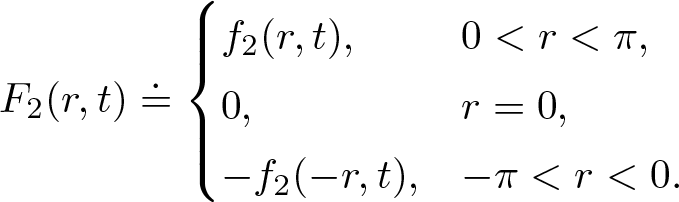 \begin{equation}
F_2
(r,t)
\doteq
\begin{cases}
f_2(r,t),
\quad
&0 \lt r \lt \pi,
\\
0,
\quad
&r=0,
\\
-f_2(-r,t),
\quad
&-\pi \lt r \lt 0.
\end{cases}
\end{equation}
\begin{equation}
F_2
(r,t)
\doteq
\begin{cases}
f_2(r,t),
\quad
&0 \lt r \lt \pi,
\\
0,
\quad
&r=0,
\\
-f_2(-r,t),
\quad
&-\pi \lt r \lt 0.
\end{cases}
\end{equation} Then, we have  $
\widehat{F}_2^r(n,t')
=
\int_{-\pi}^\pi
F_2(r,t)
e^{inr}dr
=
-\int_{-\pi}^0
f_2(-r,t)
e^{inr}dr
+
\int_{0}^\pi
f_2(r,t)
e^{inr}dr
=
i\pi
\widehat{f}_2^r(n,t').
$ Using the fact that F 2 is an odd function, we get
$
\widehat{F}_2^r(n,t')
=
\int_{-\pi}^\pi
F_2(r,t)
e^{inr}dr
=
-\int_{-\pi}^0
f_2(-r,t)
e^{inr}dr
+
\int_{0}^\pi
f_2(r,t)
e^{inr}dr
=
i\pi
\widehat{f}_2^r(n,t').
$ Using the fact that F 2 is an odd function, we get  $\widehat{F}_2^r(n,t')=-\widehat{F}_2^r(-n,t')$. Thus, working similarly as in the formula (4.12), we have
 \begin{equation}
w(r,t)
\simeq
\int_0^t
W_0(t-\tau)
f_2(\cdot,\tau)
d\tau
\simeq
\sum\limits_{n\in{\mathbb Z}}
e^{in r}
\int_0^t
e^{-i n^2 (t-t') }
\widehat{F}_2^r(n,t')
dt'.
\end{equation}
\begin{equation}
w(r,t)
\simeq
\int_0^t
W_0(t-\tau)
f_2(\cdot,\tau)
d\tau
\simeq
\sum\limits_{n\in{\mathbb Z}}
e^{in r}
\int_0^t
e^{-i n^2 (t-t') }
\widehat{F}_2^r(n,t')
dt'.
\end{equation}Also, it is derived that
 \begin{equation*}
\|f_2\|_{L^{4/3}((0,\pi)\times(0,T))}
\simeq
\|F_2\|_{L^{4/3}({\mathbb{T}}\times(0,T))}.
\end{equation*}
\begin{equation*}
\|f_2\|_{L^{4/3}((0,\pi)\times(0,T))}
\simeq
\|F_2\|_{L^{4/3}({\mathbb{T}}\times(0,T))}.
\end{equation*} Furthermore, for  $t\notin (0,T)$ we set $F_2=0$ (keeping the same notation) and we obtain
 \begin{equation}
\|f_2\|_{L^{4/3}((0,\pi)\times(0,T))}
\simeq
\|F_2\|_{L^{4/3}({\mathbb{T}}\times{\mathbb R})}.
\end{equation}
\begin{equation}
\|f_2\|_{L^{4/3}((0,\pi)\times(0,T))}
\simeq
\|F_2\|_{L^{4/3}({\mathbb{T}}\times{\mathbb R})}.
\end{equation}For the solution formula (4.18), we have the following result.
Proposition 4.3. Let  $f_2\in L^1(0,T;H^s(0,\pi))$, where $0\le s\le 2$ and $s\neq\frac12,\frac32$. Then, considering the solution defined by (4.18), the following estimates hold
 \begin{align}
\sup\limits_{t\in[0,T]}\Big\|
\int_0^t
W_0(t-t')
f_2(\cdot,t')
dt'
\Big\|_{H^{s}(0,\pi)}
\le C_{T,s}
\|f_2\|_{L^1(0,T;H^s(0,\pi))}.
\end{align}
\begin{align}
\sup\limits_{t\in[0,T]}\Big\|
\int_0^t
W_0(t-t')
f_2(\cdot,t')
dt'
\Big\|_{H^{s}(0,\pi)}
\le C_{T,s}
\|f_2\|_{L^1(0,T;H^s(0,\pi))}.
\end{align} In addition, for  $s\in {\mathbb{N}}$, if $\partial_r^sf_2\in L^{4/3}((0,\pi)\times(0,T))$, the following estimate holds:
 \begin{equation}
\Big\|\psi
\partial_r^s
\int_0^t
W_0(t-t')
f_2(\cdot,t')
dt'
\Big\|_{L^4((0,\pi)\times{\mathbb R})}
\le
C_{T}
\|\partial_r^sf_2\|_{L^{4/3}((0,\pi)\times(0,T))}.
\end{equation}
\begin{equation}
\Big\|\psi
\partial_r^s
\int_0^t
W_0(t-t')
f_2(\cdot,t')
dt'
\Big\|_{L^4((0,\pi)\times{\mathbb R})}
\le
C_{T}
\|\partial_r^sf_2\|_{L^{4/3}((0,\pi)\times(0,T))}.
\end{equation}Proof of proposition 4.3
Using the space estimate (4.15) for the homogeneous IVP (4.8), i.e.,
 \begin{align*}
\sup\limits_{t\in[0,T]}\|W_0(t)w_0\|_{H^{s}(0,\pi)}
\le C_{T,s}
\|w_0 \|_{H^s(0,\pi)},
\end{align*}
\begin{align*}
\sup\limits_{t\in[0,T]}\|W_0(t)w_0\|_{H^{s}(0,\pi)}
\le C_{T,s}
\|w_0 \|_{H^s(0,\pi)},
\end{align*}we have
 \begin{align*}
\Big\|
\int_0^t
W_0(t-t')
f_2(\cdot,t')
dt'
\Big\|_{H^{s}(0,\pi)}
\le&
\int_{t'=0}^t
\Big\|
W_0(t-t')
f_2(\cdot,t')
\Big\|_{H^{s}(0,\pi)}
dt'
\nonumber
\\
\lesssim&
\int_{t'=0}^t
\|f_2 (t') \|_{H^s(0,\pi)}
dt'
\le
\int_{t'=0}^T
\|f_2 (t') \|_{H^s(0,\pi)}
dt',
\end{align*}
\begin{align*}
\Big\|
\int_0^t
W_0(t-t')
f_2(\cdot,t')
dt'
\Big\|_{H^{s}(0,\pi)}
\le&
\int_{t'=0}^t
\Big\|
W_0(t-t')
f_2(\cdot,t')
\Big\|_{H^{s}(0,\pi)}
dt'
\nonumber
\\
\lesssim&
\int_{t'=0}^t
\|f_2 (t') \|_{H^s(0,\pi)}
dt'
\le
\int_{t'=0}^T
\|f_2 (t') \|_{H^s(0,\pi)}
dt',
\end{align*}which is the desired space estimate (4.22).
Proof of estimate (4.23) with s = 0. For this estimate, similar to the proof of estimate (4.16), we will use the formula (4.20). Also, we notice that it defines an odd function of r over  $(-\pi,\pi)$. Hence, we prove the following estimate,
 \begin{equation}
\Big\|\psi
\int_0^t
W_0(t-t')
f_2(\cdot,t')
dt'
\Big\|_{L^4({\mathbb{T}}\times{\mathbb R})}
\le
C_{T}
\|f_2\|_{L^{4/3}((0,\pi)\times(0,T))}.
\end{equation}
\begin{equation}
\Big\|\psi
\int_0^t
W_0(t-t')
f_2(\cdot,t')
dt'
\Big\|_{L^4({\mathbb{T}}\times{\mathbb R})}
\le
C_{T}
\|f_2\|_{L^{4/3}((0,\pi)\times(0,T))}.
\end{equation} To do this, using space-time Fourier transform, we express F 2 in the phase space  $(n,\lambda)$. More precisely, substituting in (4.20)
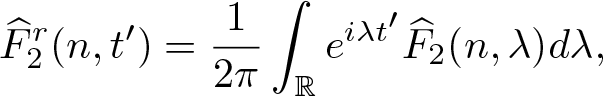 \begin{align*}
\widehat{F}_2^r(n,t')
=
\frac{1}{2\pi}\int_{\mathbb R} e^{i\lambda t'}\widehat{F}_2 (n, \lambda)d\lambda,
\end{align*}
\begin{align*}
\widehat{F}_2^r(n,t')
=
\frac{1}{2\pi}\int_{\mathbb R} e^{i\lambda t'}\widehat{F}_2 (n, \lambda)d\lambda,
\end{align*}we obtain
 \begin{align*}
\psi(t)
w(r,t)
\simeq
\psi(t)\sum\limits_{n\in{\mathbb Z}} e^{inr} \int_0^t e^{-in^2(t-t')}\int_{\lambda\in{\mathbb R}} e^{i\lambda t'}\widehat{F}_2 (n,\lambda)d\lambda dt'.
\end{align*}
\begin{align*}
\psi(t)
w(r,t)
\simeq
\psi(t)\sum\limits_{n\in{\mathbb Z}} e^{inr} \int_0^t e^{-in^2(t-t')}\int_{\lambda\in{\mathbb R}} e^{i\lambda t'}\widehat{F}_2 (n,\lambda)d\lambda dt'.
\end{align*}Performing the t ʹ integration first, it is
 \begin{align*}
\int_0^t e^{i(\lambda+n^2)t'}dt'
=
-i\frac{e^{i(\lambda+n^2)t}-1}{\lambda+n^2}.
\end{align*}
\begin{align*}
\int_0^t e^{i(\lambda+n^2)t'}dt'
=
-i\frac{e^{i(\lambda+n^2)t}-1}{\lambda+n^2}.
\end{align*} Then, the solution  $\psi(t)
w(r,t)$ becomes
$\psi(t)
w(r,t)$ becomes
 \begin{align}
\psi(t)
w(r,t)
\simeq
\psi(t)\sum\limits_{n\in{\mathbb Z}}\int_{\lambda\in{\mathbb R}} e^{inr}e^{-in^2t}\frac{e^{i(\lambda+n^2)t}-1}{\lambda+n^2}\widehat{F}_2 (n,\lambda)d\lambda.
\end{align}
\begin{align}
\psi(t)
w(r,t)
\simeq
\psi(t)\sum\limits_{n\in{\mathbb Z}}\int_{\lambda\in{\mathbb R}} e^{inr}e^{-in^2t}\frac{e^{i(\lambda+n^2)t}-1}{\lambda+n^2}\widehat{F}_2 (n,\lambda)d\lambda.
\end{align} Finally, adding and subtracting  $\psi(\lambda+n^2)$ inside the integral (localizing near the singularity $\lambda=-n^2$) gives the following decomposition of
  $\psi(t)
w(r,t)$
$\psi(t)
w(r,t)$
 \begin{align}
\psi(t)
w(r,t)
\simeq&
-\psi(t)
\sum\limits_{n\in{\mathbb Z}}\int_{\lambda\in{\mathbb R}}
e^{inr}e^{i\lambda t}
\frac{1-\psi(\lambda+n^2)}{\lambda+n^2}\widehat{F}_2 (n,\lambda)d\lambda
\end{align}
\begin{align}
\psi(t)
w(r,t)
\simeq&
-\psi(t)
\sum\limits_{n\in{\mathbb Z}}\int_{\lambda\in{\mathbb R}}
e^{inr}e^{i\lambda t}
\frac{1-\psi(\lambda+n^2)}{\lambda+n^2}\widehat{F}_2 (n,\lambda)d\lambda
\end{align} \begin{align}
&+
\psi(t)
\sum\limits_{n\in{\mathbb Z}}\int_{\lambda\in{\mathbb R}} e^{inr}e^{-in^2t}\frac{1-\psi(\lambda+n^2)}{\lambda+n^2}\widehat{F}_2 (n,\lambda)d\lambda
\end{align}
\begin{align}
&+
\psi(t)
\sum\limits_{n\in{\mathbb Z}}\int_{\lambda\in{\mathbb R}} e^{inr}e^{-in^2t}\frac{1-\psi(\lambda+n^2)}{\lambda+n^2}\widehat{F}_2 (n,\lambda)d\lambda
\end{align} \begin{align}
&-
\psi(t)\sum\limits_{n\in{\mathbb Z}}\int_{\lambda\in{\mathbb R}} e^{inr}e^{-in^2t}\frac{\psi(\lambda+n^2)(e^{i(\lambda+n^2)t}-1)}{\lambda+n^2}\widehat{F}_2 (n,\lambda)d\lambda.
\end{align}
\begin{align}
&-
\psi(t)\sum\limits_{n\in{\mathbb Z}}\int_{\lambda\in{\mathbb R}} e^{inr}e^{-in^2t}\frac{\psi(\lambda+n^2)(e^{i(\lambda+n^2)t}-1)}{\lambda+n^2}\widehat{F}_2 (n,\lambda)d\lambda.
\end{align}Estimate for (4.28). Let
 \begin{align*}
f(r,t)
=
\sum\limits_{n\in{\mathbb Z}}\int_{{\mathbb R}}
e^{inr}e^{i\lambda t}
\frac{1-\psi(\lambda+n^2)}{\lambda+n^2}
\widehat{F}_2(n,\lambda) d\lambda.
\end{align*}
\begin{align*}
f(r,t)
=
\sum\limits_{n\in{\mathbb Z}}\int_{{\mathbb R}}
e^{inr}e^{i\lambda t}
\frac{1-\psi(\lambda+n^2)}{\lambda+n^2}
\widehat{F}_2(n,\lambda) d\lambda.
\end{align*} Since  $\psi\in C_0^\infty({\mathbb R})$, we have
 \begin{align*}
\|(4.28)\|_{L^4({\mathbb{T}}\times{\mathbb R})}
\simeq
\|\psi(\cdot)f(\cdot,\cdot)\|_{L^4({\mathbb{T}}\times{\mathbb R})}
\leq
\|\psi\|_{L^\infty_t}\|f\|_{L^4({\mathbb{T}}\times{\mathbb R})}.
\end{align*}
\begin{align*}
\|(4.28)\|_{L^4({\mathbb{T}}\times{\mathbb R})}
\simeq
\|\psi(\cdot)f(\cdot,\cdot)\|_{L^4({\mathbb{T}}\times{\mathbb R})}
\leq
\|\psi\|_{L^\infty_t}\|f\|_{L^4({\mathbb{T}}\times{\mathbb R})}.
\end{align*}Also, computing the Fourier transform of f with respect to r gives
 \begin{align*}
\widehat{f}^r(n,t)
\simeq
\int_{{\mathbb R}}
e^{i\lambda t}
\frac{1-\psi(\lambda+n^2)}{\lambda+n^2}
\widehat{F}_2(n,\lambda) d\lambda.
\end{align*}
\begin{align*}
\widehat{f}^r(n,t)
\simeq
\int_{{\mathbb R}}
e^{i\lambda t}
\frac{1-\psi(\lambda+n^2)}{\lambda+n^2}
\widehat{F}_2(n,\lambda) d\lambda.
\end{align*}Therefore,
 \begin{align*}
\widehat f(n,\lambda)
=
\frac{1-\psi(\lambda+n^2)}{\lambda+n^2}\widehat{F}_2(n,\lambda).
\end{align*}
\begin{align*}
\widehat f(n,\lambda)
=
\frac{1-\psi(\lambda+n^2)}{\lambda+n^2}\widehat{F}_2(n,\lambda).
\end{align*}Now, we need the following result, which is provided in [Reference Bourgain8].
Proposition 4.4. If the multiplier  $M=M(n,\lambda)$ satisfies
 \begin{equation}
|M(n,\lambda)|
\lesssim
(1+|\lambda+n^2|)^{-\frac34},
\quad
\text{for all}
\quad
n\in{\mathbb Z}
\quad
\text{and}
\quad
\lambda\in {\mathbb R},
\end{equation}
\begin{equation}
|M(n,\lambda)|
\lesssim
(1+|\lambda+n^2|)^{-\frac34},
\quad
\text{for all}
\quad
n\in{\mathbb Z}
\quad
\text{and}
\quad
\lambda\in {\mathbb R},
\end{equation} then M acts boundedly from  $L^{4/3}({\mathbb Z}\times{\mathbb R})$ to $L^4({\mathbb Z}\times{\mathbb R})$, that is
 \begin{equation}
\left\|
\sum\limits_{n=1}^\infty
e^{inr}
\int_{{\mathbb R}}
M(n,\lambda)
\widehat{f}(n,\lambda)
e^{i\lambda t}
d\lambda
\right\|_{L^{4}({\mathbb{T}}\times{\mathbb R})}
\lesssim
\|f\|_{L^{4/3}({\mathbb{T}}\times{\mathbb R})}.
\end{equation}
\begin{equation}
\left\|
\sum\limits_{n=1}^\infty
e^{inr}
\int_{{\mathbb R}}
M(n,\lambda)
\widehat{f}(n,\lambda)
e^{i\lambda t}
d\lambda
\right\|_{L^{4}({\mathbb{T}}\times{\mathbb R})}
\lesssim
\|f\|_{L^{4/3}({\mathbb{T}}\times{\mathbb R})}.
\end{equation} Proposition 4.4 is due to lemma 4.2 and duality (see corollary 4.5). Now, from this, we finish the proof of estimate (4.25) for (4.28). In fact, by the definition of  $\psi(t)$, the integrand is non-zero only for $|\lambda+n^2|\geq \frac12$. Therefore, $1+|\lambda+n^2|\leq 2 |\lambda+n^2|+|\lambda+n^2|=3|\lambda+n^2|$ and so
 \begin{align*}
\|f\|_{L^4({\mathbb{T}}\times{\mathbb R})}
\lesssim
\|F_2\|_{L^{4/3}({\mathbb{T}}\times{\mathbb R})},
\end{align*}
\begin{align*}
\|f\|_{L^4({\mathbb{T}}\times{\mathbb R})}
\lesssim
\|F_2\|_{L^{4/3}({\mathbb{T}}\times{\mathbb R})},
\end{align*}which, together with the inequality (4.21), gives us the desired estimate (4.25) for term (4.28).
Estimate for (4.29). To estimate  $\|(4.29)\|_{L^4({\mathbb{T}}\times {\mathbb R})}$, we first find the Fourier transform of the function
 \begin{align*}
f(r,t)
=
(4.29)
=
\psi(t)
\sum\limits_{n\in{\mathbb Z}}\int_{\mathbb{R}}
e^{i(n r+n^2t)}
\frac{1-\psi(\lambda+n^2)}{\lambda+n^2}
\widehat{F}_2(n,\lambda) d\lambda .
\end{align*}
\begin{align*}
f(r,t)
=
(4.29)
=
\psi(t)
\sum\limits_{n\in{\mathbb Z}}\int_{\mathbb{R}}
e^{i(n r+n^2t)}
\frac{1-\psi(\lambda+n^2)}{\lambda+n^2}
\widehat{F}_2(n,\lambda) d\lambda .
\end{align*} It is clearly seen that  $
\widehat f^r(n,t)
\simeq
\psi(t)e^{in^2 t}C_n,
$ where
$
\widehat f^r(n,t)
\simeq
\psi(t)e^{in^2 t}C_n,
$ where
 \begin{align*}
C_n
=
\int_{\mathbb R}
\frac{1-\psi(\lambda+n^2)}{\lambda+n^2}\widehat{F}_2(n,\lambda)d\lambda.
\end{align*}
\begin{align*}
C_n
=
\int_{\mathbb R}
\frac{1-\psi(\lambda+n^2)}{\lambda+n^2}\widehat{F}_2(n,\lambda)d\lambda.
\end{align*} Then, computing the Fourier transform of  $\widehat f^r$ with respect to t gives
 \begin{align*}
\widehat f(n,\lambda)
=
C_n\widehat \psi(\lambda+n^2).
\end{align*}
\begin{align*}
\widehat f(n,\lambda)
=
C_n\widehat \psi(\lambda+n^2).
\end{align*}Applying estimate (4.17), it is obtained that
 \begin{align}
\|(4.29)\|_{L^4({\mathbb{T}}\times {\mathbb R})}
\lesssim&
\|(1+|\lambda+n^2|)^{\frac{3}{8}}
C_n\widehat \psi(\lambda+n^2)
\|_{L^2({\mathbb Z}\times{\mathbb R})}
\nonumber
\\
=&
\left(
\sum\limits_{n\in{\mathbb Z}}
\int_{\lambda\in{\mathbb R}}
(1+|\lambda+n^2|)^{3/4}
|C_n\hat \psi(\lambda+n^2)|^2d\lambda
\right)^\frac12
\nonumber
\\
\lesssim&
\left(
\sum\limits_{n\in{\mathbb Z}}
|C_n|^2
\right)^\frac12
=
\left(
\sum\limits_{n\in{\mathbb Z}}
\Big|
\int_{\mathbb R}
\frac{1-\psi(\lambda+n^2)}{\lambda+n^2}\widehat{F}_2(n,\lambda)d\lambda
\Big|^2
\right)^\frac12.
\end{align}
\begin{align}
\|(4.29)\|_{L^4({\mathbb{T}}\times {\mathbb R})}
\lesssim&
\|(1+|\lambda+n^2|)^{\frac{3}{8}}
C_n\widehat \psi(\lambda+n^2)
\|_{L^2({\mathbb Z}\times{\mathbb R})}
\nonumber
\\
=&
\left(
\sum\limits_{n\in{\mathbb Z}}
\int_{\lambda\in{\mathbb R}}
(1+|\lambda+n^2|)^{3/4}
|C_n\hat \psi(\lambda+n^2)|^2d\lambda
\right)^\frac12
\nonumber
\\
\lesssim&
\left(
\sum\limits_{n\in{\mathbb Z}}
|C_n|^2
\right)^\frac12
=
\left(
\sum\limits_{n\in{\mathbb Z}}
\Big|
\int_{\mathbb R}
\frac{1-\psi(\lambda+n^2)}{\lambda+n^2}\widehat{F}_2(n,\lambda)d\lambda
\Big|^2
\right)^\frac12.
\end{align} Furthermore, for the  $d\lambda$-integral in the above estimate, applying the Cauchy–Schwarz inequality gives
 \begin{align}
\left |
\int_{\mathbb R}
\frac{1-\psi(\lambda+n^2)}{\lambda+n^2}\widehat{F}_2(n,\lambda)d\lambda
\right |^2
\le&
\int_{\mathbb R}
\Big |
\frac{1-\psi(\lambda+n^2)}{\lambda+n^2}
\Big|^{5/4}
d\lambda
\nonumber
\\
&\cdot
\int_{\mathbb R}
\Big|
\frac{1-\psi(\lambda+n^2)}{\lambda+n^2}
\Big|^{3/4}
|\widehat{F}_2(n,\lambda)|^2
d\lambda
\nonumber
\\
\lesssim&
\int_{\mathbb R}
(1+|\lambda+n^2|)^{-3/4}
|\widehat{F}_2(n,\lambda)|^2
d\lambda.
\end{align}
\begin{align}
\left |
\int_{\mathbb R}
\frac{1-\psi(\lambda+n^2)}{\lambda+n^2}\widehat{F}_2(n,\lambda)d\lambda
\right |^2
\le&
\int_{\mathbb R}
\Big |
\frac{1-\psi(\lambda+n^2)}{\lambda+n^2}
\Big|^{5/4}
d\lambda
\nonumber
\\
&\cdot
\int_{\mathbb R}
\Big|
\frac{1-\psi(\lambda+n^2)}{\lambda+n^2}
\Big|^{3/4}
|\widehat{F}_2(n,\lambda)|^2
d\lambda
\nonumber
\\
\lesssim&
\int_{\mathbb R}
(1+|\lambda+n^2|)^{-3/4}
|\widehat{F}_2(n,\lambda)|^2
d\lambda.
\end{align}Now, we need the following dual estimate of lemma 4.2 (see [Reference Bourgain8]).
Corollary 4.5. For any test function f, we have
 \begin{equation}
\|(1+|\lambda+n^2|)^{-\frac{3}{8}}\widehat{f}\|_{L^2({\mathbb Z}\times{\mathbb R})}
\le
c
\|f\|_{L^{4/3}({\mathbb{T}}\times{\mathbb R})}.
\end{equation}
\begin{equation}
\|(1+|\lambda+n^2|)^{-\frac{3}{8}}\widehat{f}\|_{L^2({\mathbb Z}\times{\mathbb R})}
\le
c
\|f\|_{L^{4/3}({\mathbb{T}}\times{\mathbb R})}.
\end{equation}Finally, combining estimates (4.33) and (4.34) with corollary 4.5 and using estimate (4.21), it is deduced that
 \begin{align*}
\|(4.29)\|_{L^4({\mathbb{T}}\times {\mathbb R})}
\lesssim&
\left(
\sum\limits_{n\in{\mathbb Z}}
\int_{\mathbb R}
(1+|\lambda+n^2|)^{-3/4}
|\widehat{F}_2(n,\lambda)|^2
d\lambda
\right)^\frac12\\&
=
\|(1+|\lambda+n^2|)^{-\frac{3}{8}}\widehat{F}_2\|_{L^2({\mathbb Z}\times{\mathbb R})}
\\
\lesssim&
\|F_2\|_{L^{4/3}({\mathbb{T}}\times{\mathbb R})}
\simeq
\|f_2\|_{L^{4/3}({\mathbb{T}}\times(0,T))}.
\end{align*}
\begin{align*}
\|(4.29)\|_{L^4({\mathbb{T}}\times {\mathbb R})}
\lesssim&
\left(
\sum\limits_{n\in{\mathbb Z}}
\int_{\mathbb R}
(1+|\lambda+n^2|)^{-3/4}
|\widehat{F}_2(n,\lambda)|^2
d\lambda
\right)^\frac12\\&
=
\|(1+|\lambda+n^2|)^{-\frac{3}{8}}\widehat{F}_2\|_{L^2({\mathbb Z}\times{\mathbb R})}
\\
\lesssim&
\|F_2\|_{L^{4/3}({\mathbb{T}}\times{\mathbb R})}
\simeq
\|f_2\|_{L^{4/3}({\mathbb{T}}\times(0,T))}.
\end{align*}This completes the estimate for (4.29).
Estimate for (4.30). From Taylor’s series at  $\lambda+n^2=0$, we can expand
 \begin{equation*}
e^{i(\lambda+n^2)t}-1
=
\sum\limits_{k=1}^\infty
\frac{t^k(\lambda+n^2)^k}{k!}.
\end{equation*}
\begin{equation*}
e^{i(\lambda+n^2)t}-1
=
\sum\limits_{k=1}^\infty
\frac{t^k(\lambda+n^2)^k}{k!}.
\end{equation*} Thus,  $(4.30)\simeq\sum\limits_{k=1}^\infty \frac{i^{k+1}}{k!}f_k$, where
 \begin{align*}
f_k(r,t)
\doteq
t^k \psi(t)
\sum\limits_{n\in{\mathbb Z}}\int_{\mathbb{R}}
e^{inr}e^{-in^2t}
\psi(\lambda+n^2)(\lambda+n^2)^{k-1}
\widehat{F}_2(n,\lambda) d\lambda\, .
\end{align*}
\begin{align*}
f_k(r,t)
\doteq
t^k \psi(t)
\sum\limits_{n\in{\mathbb Z}}\int_{\mathbb{R}}
e^{inr}e^{-in^2t}
\psi(\lambda+n^2)(\lambda+n^2)^{k-1}
\widehat{F}_2(n,\lambda) d\lambda\, .
\end{align*}The Fourier transform of the function fk yields
 \begin{align*}
\widehat f^r_k(n,t)
=
C_k(n)t^k\psi(t)e^{-in^2t},
\end{align*}
\begin{align*}
\widehat f^r_k(n,t)
=
C_k(n)t^k\psi(t)e^{-in^2t},
\end{align*}where
 \begin{align*}
C_k(n)
=
\int_{\mathbb{R}}
\psi(\lambda+n^2)(\lambda +n^2)^{k-1}
\widehat{F}_2(n,\lambda) d\lambda.
\end{align*}
\begin{align*}
C_k(n)
=
\int_{\mathbb{R}}
\psi(\lambda+n^2)(\lambda +n^2)^{k-1}
\widehat{F}_2(n,\lambda) d\lambda.
\end{align*}Therefore,
 \begin{align*}
\widehat f_k(n,\lambda)
=
C_k(n)\widehat{t^k\psi}(\lambda+n^2).
\end{align*}
\begin{align*}
\widehat f_k(n,\lambda)
=
C_k(n)\widehat{t^k\psi}(\lambda+n^2).
\end{align*} Let us now estimate (4.30) using the expression of  $\widehat f_k(n,\lambda)$.
 \begin{align}
\|(4.30)\|_{L^4({\mathbb{T}}\times {\mathbb R})}
\lesssim&
\left\|\sum\limits_{k=1}^\infty\frac{i^{k+1}}{k!}f_k\right\|_{L^4({\mathbb{T}}\times {\mathbb R})}
\lesssim
\sum\limits_{k=1}^\infty\frac{1}{k!}\left\|f_k\right\|_{L^4({\mathbb{T}}\times {\mathbb R})}.
\end{align}
\begin{align}
\|(4.30)\|_{L^4({\mathbb{T}}\times {\mathbb R})}
\lesssim&
\left\|\sum\limits_{k=1}^\infty\frac{i^{k+1}}{k!}f_k\right\|_{L^4({\mathbb{T}}\times {\mathbb R})}
\lesssim
\sum\limits_{k=1}^\infty\frac{1}{k!}\left\|f_k\right\|_{L^4({\mathbb{T}}\times {\mathbb R})}.
\end{align}Applying estimate (4.17), we obtain
 \begin{align}
\|f_k\|_{L^4({\mathbb{T}}\times {\mathbb R})}
\lesssim&
\|(1+|\lambda+n^2|)^{\frac{3}{8}}
C_k(n)\widehat{t^k \psi}(\lambda+n^2)
\|_{L^2({\mathbb Z}\times{\mathbb R})}
\nonumber
\\
=&
\left(
\sum\limits_{n\in{\mathbb Z}}
\int_{\lambda\in{\mathbb R}}
(1+|\lambda+n^2|)^{3/4}
|C_k(n)\widehat{t^k \psi}(\lambda+n^2)|^2d\lambda
\right)^\frac12
\nonumber
\\
\lesssim&
\left(
\sum\limits_{n\in{\mathbb Z}}
|C_k(n)|^2
\right)^\frac12
=
\left(
\sum\limits_{n\in{\mathbb Z}}
\Big|
\int_{\mathbb{R}}
\psi(\lambda+n^2)(\lambda +n^2)^{k-1}
\widehat{F}_2(n,\lambda) d\lambda
\Big|^2
\right)^\frac12.
\end{align}
\begin{align}
\|f_k\|_{L^4({\mathbb{T}}\times {\mathbb R})}
\lesssim&
\|(1+|\lambda+n^2|)^{\frac{3}{8}}
C_k(n)\widehat{t^k \psi}(\lambda+n^2)
\|_{L^2({\mathbb Z}\times{\mathbb R})}
\nonumber
\\
=&
\left(
\sum\limits_{n\in{\mathbb Z}}
\int_{\lambda\in{\mathbb R}}
(1+|\lambda+n^2|)^{3/4}
|C_k(n)\widehat{t^k \psi}(\lambda+n^2)|^2d\lambda
\right)^\frac12
\nonumber
\\
\lesssim&
\left(
\sum\limits_{n\in{\mathbb Z}}
|C_k(n)|^2
\right)^\frac12
=
\left(
\sum\limits_{n\in{\mathbb Z}}
\Big|
\int_{\mathbb{R}}
\psi(\lambda+n^2)(\lambda +n^2)^{k-1}
\widehat{F}_2(n,\lambda) d\lambda
\Big|^2
\right)^\frac12.
\end{align} Furthermore, for the  $d\lambda$-integral in the above estimate, the Cauchy–Schwartz inequality gives
 \begin{align}
&\Big|
\int_{\mathbb R}
\psi(\lambda+n^2)(\lambda +n^2)^{k-1}\widehat{F}_2(n,\lambda)d\lambda
\Big|^2
\nonumber
\\
\le&
\int_{\mathbb R}
|\psi(\lambda+n^2)(\lambda +n^2)^{k-1}|^2
(1+|\lambda+n^2|)^{3/4}
d\lambda
\cdot
\int_{\mathbb R}
(1+|\lambda+n^2|)^{-3/4}
|\widehat{F}_2(n,\lambda)|^2
d\lambda
\nonumber
\\
\lesssim&
\int_{\mathbb R}
(1+|\lambda+n^2|)^{-3/4}
|\widehat{F}_2(n,\lambda)|^2
d\lambda.
\end{align}
\begin{align}
&\Big|
\int_{\mathbb R}
\psi(\lambda+n^2)(\lambda +n^2)^{k-1}\widehat{F}_2(n,\lambda)d\lambda
\Big|^2
\nonumber
\\
\le&
\int_{\mathbb R}
|\psi(\lambda+n^2)(\lambda +n^2)^{k-1}|^2
(1+|\lambda+n^2|)^{3/4}
d\lambda
\cdot
\int_{\mathbb R}
(1+|\lambda+n^2|)^{-3/4}
|\widehat{F}_2(n,\lambda)|^2
d\lambda
\nonumber
\\
\lesssim&
\int_{\mathbb R}
(1+|\lambda+n^2|)^{-3/4}
|\widehat{F}_2(n,\lambda)|^2
d\lambda.
\end{align}Finally, combining estimates (4.36), (4.37), and (4.38) with corollary 4.5 and using estimate (4.21), it is obtained that
 \begin{align*}
\|(4.30)\|_{L^4({\mathbb{T}}\times {\mathbb R})}
\lesssim&
\sum\limits_{k=1}^\infty\frac{1}{k!}
\left(
\sum\limits_{n\in{\mathbb Z}}
\int_{\mathbb R}
(1+|\lambda+n^2|)^{-3/4}
|\widehat{F}_2(n,\lambda)|^2
d\lambda
\right)^\frac12
\\
\lesssim&
\|(1+|\lambda+n^2|)^{-\frac{3}{8}}\widehat{F}_2\|_{L^2({\mathbb Z}\times{\mathbb R})}
\\
\lesssim&
\|F_2\|_{L^{4/3}({\mathbb{T}}\times{\mathbb R})}
\simeq
\|f_2\|_{L^{4/3}({\mathbb{T}}\times(0,T))}.
\end{align*}
\begin{align*}
\|(4.30)\|_{L^4({\mathbb{T}}\times {\mathbb R})}
\lesssim&
\sum\limits_{k=1}^\infty\frac{1}{k!}
\left(
\sum\limits_{n\in{\mathbb Z}}
\int_{\mathbb R}
(1+|\lambda+n^2|)^{-3/4}
|\widehat{F}_2(n,\lambda)|^2
d\lambda
\right)^\frac12
\\
\lesssim&
\|(1+|\lambda+n^2|)^{-\frac{3}{8}}\widehat{F}_2\|_{L^2({\mathbb Z}\times{\mathbb R})}
\\
\lesssim&
\|F_2\|_{L^{4/3}({\mathbb{T}}\times{\mathbb R})}
\simeq
\|f_2\|_{L^{4/3}({\mathbb{T}}\times(0,T))}.
\end{align*}We complete the proof of estimate (4.23) with s = 0.
Proof of estimate (4.23) with  $s\in {\mathbb{N}}^+$. Consider the periodic function $F_2(r,t)$. Employing integration by parts, we can express the Fourier transform of the spatial derivative $\partial_r^s F_2$ as
 \begin{equation*}
\widehat{\partial_r^s F}_2^r(n,t')
\simeq
n^s
\widehat{F}_2^r(n,t').
\end{equation*}
\begin{equation*}
\widehat{\partial_r^s F}_2^r(n,t')
\simeq
n^s
\widehat{F}_2^r(n,t').
\end{equation*}Utilizing this result and the complex formula (4.20), we derive
 \begin{align*}
\partial_r^s \int_0^t
W_0(t-\tau)
f_2(\cdot,\tau)
d\tau &
\simeq
\sum\limits_{n\in{\mathbb Z}}
e^{in r}
n^s
\int_0^t
e^{-i n^2 (t-t') }
\widehat{F}_2^r(n,t')
dt'\\ &
\simeq
\sum\limits_{n\in{\mathbb Z}}
e^{in r}
\int_0^t
e^{-i n^2 (t-t') }
\widehat{\partial_r^s F}_2^r(n,t')
dt'.
\end{align*}
\begin{align*}
\partial_r^s \int_0^t
W_0(t-\tau)
f_2(\cdot,\tau)
d\tau &
\simeq
\sum\limits_{n\in{\mathbb Z}}
e^{in r}
n^s
\int_0^t
e^{-i n^2 (t-t') }
\widehat{F}_2^r(n,t')
dt'\\ &
\simeq
\sum\limits_{n\in{\mathbb Z}}
e^{in r}
\int_0^t
e^{-i n^2 (t-t') }
\widehat{\partial_r^s F}_2^r(n,t')
dt'.
\end{align*} Consequently, by applying estimate (4.23) with s = 0 for  $\partial_r^s F_2$, we obtain the desired estimate (4.23) with $s\in{\mathbb{N}}^+$. The proof of proposition 4.3 is completed. $\square$
Solving the ibvp (4.7). For this problem, the solution is given by the following formula, which is provided in [Reference Bona, Sun and Zhang7]
 \begin{align}
u(r,t)&
=
2\pi i
\sum\limits_{n=1}^\infty
n
\sin (n r)
\int_0^t
e^{-i n^2 (t-t') }
[h_1(t')-(-1)^nh_2(t')]
dt'\\&
=
\int_0^t W_0(t-t')q(\cdot, t')dt',
\end{align}
\begin{align}
u(r,t)&
=
2\pi i
\sum\limits_{n=1}^\infty
n
\sin (n r)
\int_0^t
e^{-i n^2 (t-t') }
[h_1(t')-(-1)^nh_2(t')]
dt'\\&
=
\int_0^t W_0(t-t')q(\cdot, t')dt',
\end{align}where
 \begin{equation}
q(x,t)
\doteq
2\pi i
\Big[
\sum\limits_{n=1}^\infty n
\sin (nx)
h_1(t)
-
\sum\limits_{n=1}^\infty
(-1)^n n
\sin (nx)
h_2(t)
\Big].
\end{equation}
\begin{equation}
q(x,t)
\doteq
2\pi i
\Big[
\sum\limits_{n=1}^\infty n
\sin (nx)
h_1(t)
-
\sum\limits_{n=1}^\infty
(-1)^n n
\sin (nx)
h_2(t)
\Big].
\end{equation}Next, we define the following boundary operator
 \begin{equation}
W_b
h
\doteq
2 i
\sum\limits_{n=1}^\infty
n
\sin (n r)
\int_0^t
e^{-i n^2 (t-t') }
h(t')
dt',
\end{equation}
\begin{equation}
W_b
h
\doteq
2 i
\sum\limits_{n=1}^\infty
n
\sin (n r)
\int_0^t
e^{-i n^2 (t-t') }
h(t')
dt',
\end{equation}which has the form
 \begin{equation}
W_b
h
=
\sum\limits_{n\in{\mathbb Z}}
ne^{inr}
\int_0^t
e^{-i n^2 (t-t') }
h(t')
dt',
\quad
r\in {\mathbb{T}},
t\in{\mathbb R}.
\end{equation}
\begin{equation}
W_b
h
=
\sum\limits_{n\in{\mathbb Z}}
ne^{inr}
\int_0^t
e^{-i n^2 (t-t') }
h(t')
dt',
\quad
r\in {\mathbb{T}},
t\in{\mathbb R}.
\end{equation}The following result can be proved.
Proposition 4.6. Let  $h\in H^{1/2}_{00}(0,T)$. Then, the solution defined by (4.41) satisfies the following estimates
 \begin{align}
\sup\limits_{t\in[0,T]}\Big\|
\psi
W_b
h
\Big\|_{L^2({\mathbb{T}})}
\lesssim
\|h\|_{H^{1/2}(0,T)},
\end{align}
\begin{align}
\sup\limits_{t\in[0,T]}\Big\|
\psi
W_b
h
\Big\|_{L^2({\mathbb{T}})}
\lesssim
\|h\|_{H^{1/2}(0,T)},
\end{align} \begin{align}
\Big\|\psi
W_b h
\Big\|_{L^4({\mathbb{T}}\times{\mathbb R})}
\lesssim
\|h\|_{H^{1/2}(0,T)}.
\end{align}
\begin{align}
\Big\|\psi
W_b h
\Big\|_{L^4({\mathbb{T}}\times{\mathbb R})}
\lesssim
\|h\|_{H^{1/2}(0,T)}.
\end{align} In addition, for  $0\le s\le 2$, if $h\in H_0^{\frac{s+1}{2}}(0,T)$ (for s an even integer $h\in H_{00}^{\frac{s+1}{2}}(0,T)$), then we have
 \begin{equation}
\sup\limits_{t\in[0,T]}\Big\|
\psi
\partial_r^s
W_b
h
\Big\|_{L^2({\mathbb{T}})}
+
\Big\|\psi
\partial_r^s W_b h
\Big\|_{L^4({\mathbb{T}}\times{\mathbb R})}
\lesssim
\|h\|_{H^{(s+1)/2}(0,T)}.
\end{equation}
\begin{equation}
\sup\limits_{t\in[0,T]}\Big\|
\psi
\partial_r^s
W_b
h
\Big\|_{L^2({\mathbb{T}})}
+
\Big\|\psi
\partial_r^s W_b h
\Big\|_{L^4({\mathbb{T}}\times{\mathbb R})}
\lesssim
\|h\|_{H^{(s+1)/2}(0,T)}.
\end{equation}Proof of proposition 4.6
The proof of this proposition is similar to the proof of proposition 4.3 and was also given in [Reference Bona, Sun and Zhang7] (see propositions 4.7 and 4.8). Here, we only provide the proof for estimates (4.43) and (4.44), and we give a different proof by modifying and simplifying the proof in [Reference Bona, Sun and Zhang7]. We start with writing  $h(t')=\frac1{2\pi}\int_{{\mathbb R}}e^{i\lambda t'}\widehat{h}(\lambda)d\lambda$, which, together with formula (4.42), implies
 \begin{equation}
\psi
\cdot
W_b
h
=
\frac{\psi(t)}{2\pi}
\sum\limits_{n=-\infty}^\infty
ne^{inr}
\int_0^t
e^{-i n^2 (t-t') }
\int_{{\mathbb R}}e^{i\lambda t'}\widehat{h}(\lambda)d\lambda
dt'.
\end{equation}
\begin{equation}
\psi
\cdot
W_b
h
=
\frac{\psi(t)}{2\pi}
\sum\limits_{n=-\infty}^\infty
ne^{inr}
\int_0^t
e^{-i n^2 (t-t') }
\int_{{\mathbb R}}e^{i\lambda t'}\widehat{h}(\lambda)d\lambda
dt'.
\end{equation}Performing the t ʹ integration first gives
 \begin{align*}
\int_0^t e^{i(\lambda+n^2)t'}dt'
=
-i\frac{e^{i(\lambda+n^2)t}-1}{\lambda+n^2}.
\end{align*}
\begin{align*}
\int_0^t e^{i(\lambda+n^2)t'}dt'
=
-i\frac{e^{i(\lambda+n^2)t}-1}{\lambda+n^2}.
\end{align*} Then, the above solution  $\psi(t)
w(r,t)$ becomes
$\psi(t)
w(r,t)$ becomes
 \begin{align}
\psi(t)
W_b
h(r,t)
=
-
\frac{i\psi(t)}{2\pi}\sum\limits_{n\in{\mathbb Z}}\int_{\lambda\in{\mathbb R}} e^{inr}e^{-in^2t}\frac{e^{i(\lambda+n^2)t}-1}{\lambda+n^2}
\cdot
n\widehat{h}(\lambda)d\lambda
=
I^{+}+I^{-},
\end{align}
\begin{align}
\psi(t)
W_b
h(r,t)
=
-
\frac{i\psi(t)}{2\pi}\sum\limits_{n\in{\mathbb Z}}\int_{\lambda\in{\mathbb R}} e^{inr}e^{-in^2t}\frac{e^{i(\lambda+n^2)t}-1}{\lambda+n^2}
\cdot
n\widehat{h}(\lambda)d\lambda
=
I^{+}+I^{-},
\end{align} where  $I^{+}$ is the integral over $(0,\infty)$ and $I^{-}$ is the integral over $(-\infty,0)$. More precisely, we have
 \begin{align}
I^{+}
\doteq&
-
\frac{i\psi(t)}{2\pi}\sum\limits_{n\in{\mathbb Z}}\int_{0}^\infty e^{inr}e^{-in^2t}\frac{e^{i(\lambda+n^2)t}-1}{\lambda+n^2}
\cdot
n\widehat{h}(\lambda)d\lambda,
\end{align}
\begin{align}
I^{+}
\doteq&
-
\frac{i\psi(t)}{2\pi}\sum\limits_{n\in{\mathbb Z}}\int_{0}^\infty e^{inr}e^{-in^2t}\frac{e^{i(\lambda+n^2)t}-1}{\lambda+n^2}
\cdot
n\widehat{h}(\lambda)d\lambda,
\end{align} \begin{align}
I^{-}
\doteq&
-
\frac{i\psi(t)}{2\pi}\sum\limits_{n\in{\mathbb Z}}\int_{-\infty}^0 e^{inr}e^{-in^2t}\frac{e^{i(\lambda+n^2)t}-1}{\lambda+n^2}
\cdot
n\widehat{h}(\lambda)d\lambda.
\end{align}
\begin{align}
I^{-}
\doteq&
-
\frac{i\psi(t)}{2\pi}\sum\limits_{n\in{\mathbb Z}}\int_{-\infty}^0 e^{inr}e^{-in^2t}\frac{e^{i(\lambda+n^2)t}-1}{\lambda+n^2}
\cdot
n\widehat{h}(\lambda)d\lambda.
\end{align} To estimate  $I^{+}$, we split it as $I^{+}=I_1^{+}-I_2^{+}$, where
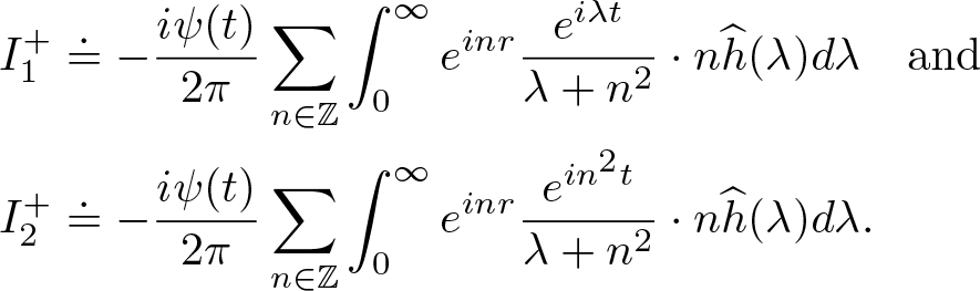 \begin{align*}
I_1^{+}&
\doteq
-
\frac{i\psi(t)}{2\pi}\sum\limits_{n\in{\mathbb Z}}\int_{0}^\infty e^{inr}\frac{e^{i\lambda t}}{\lambda+n^2}
\cdot
n\widehat{h}(\lambda)d\lambda
\quad
\text{and}\\
I_2^{+}&
\doteq
-
\frac{i\psi(t)}{2\pi}\sum\limits_{n\in{\mathbb Z}}\int_{0}^\infty e^{inr}\frac{e^{in^2 t}}{\lambda+n^2}
\cdot
n\widehat{h}(\lambda)d\lambda.
\end{align*}
\begin{align*}
I_1^{+}&
\doteq
-
\frac{i\psi(t)}{2\pi}\sum\limits_{n\in{\mathbb Z}}\int_{0}^\infty e^{inr}\frac{e^{i\lambda t}}{\lambda+n^2}
\cdot
n\widehat{h}(\lambda)d\lambda
\quad
\text{and}\\
I_2^{+}&
\doteq
-
\frac{i\psi(t)}{2\pi}\sum\limits_{n\in{\mathbb Z}}\int_{0}^\infty e^{inr}\frac{e^{in^2 t}}{\lambda+n^2}
\cdot
n\widehat{h}(\lambda)d\lambda.
\end{align*} Estimate for  $I_1^{+}$. Let
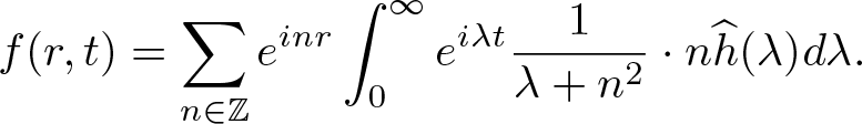 \begin{equation*}
f(r,t)
=
\sum\limits_{n\in{\mathbb Z}}
e^{inr}
\int_{0}^\infty
e^{i\lambda t}
\frac{1}{\lambda+n^2}\cdot
n\widehat{h}(\lambda)
d\lambda.
\end{equation*}
\begin{equation*}
f(r,t)
=
\sum\limits_{n\in{\mathbb Z}}
e^{inr}
\int_{0}^\infty
e^{i\lambda t}
\frac{1}{\lambda+n^2}\cdot
n\widehat{h}(\lambda)
d\lambda.
\end{equation*} First, we prove L 2 estimate (4.43) for  $I_1^{+}$. Since ψ is compactly supported in $(0,1)$, we have
 \begin{equation*}\sup\limits_{t\in[0,T]}\|I_1^{+}\|_{L^2({\mathbb{T}})}\le \sup\limits_{t\in[0,1]}\|f\|_{L^2({\mathbb{T}})}. \end{equation*}
Taking the Fourier transform with respect to r yields
 \begin{equation}
\widehat{f}^r
(n,t)
\simeq
\int_{0}^\infty
e^{i\lambda t}
\frac{1}{\lambda+n^2}\cdot
n\widehat{h}(\lambda)
d\lambda,
\end{equation}
\begin{equation}
\widehat{f}^r
(n,t)
\simeq
\int_{0}^\infty
e^{i\lambda t}
\frac{1}{\lambda+n^2}\cdot
n\widehat{h}(\lambda)
d\lambda,
\end{equation}which, by Plancherel theorem, implies that
 \begin{align}
\|f\|_{L^2({\mathbb{T}})}^2
\lesssim&
\sum\limits_{n\in{\mathbb Z}}
\Big|
\int_{0}^\infty
e^{i\lambda t}
\frac{1}{\lambda+n^2}\cdot
n\widehat{h}(\lambda)
d\lambda
\Big|^2
\le
\sum\limits_{n\in{\mathbb Z}}
\Big[
\int_{0}^\infty
\Big|
\frac{1}{\lambda+n^2}\cdot
n\widehat{h}(\lambda)
\Big|
d\lambda
\Big]^2.
\end{align}
\begin{align}
\|f\|_{L^2({\mathbb{T}})}^2
\lesssim&
\sum\limits_{n\in{\mathbb Z}}
\Big|
\int_{0}^\infty
e^{i\lambda t}
\frac{1}{\lambda+n^2}\cdot
n\widehat{h}(\lambda)
d\lambda
\Big|^2
\le
\sum\limits_{n\in{\mathbb Z}}
\Big[
\int_{0}^\infty
\Big|
\frac{1}{\lambda+n^2}\cdot
n\widehat{h}(\lambda)
\Big|
d\lambda
\Big]^2.
\end{align} Now, applying Cauchy–Schwarz inequality in  $d\lambda$, for ɛ > 0 and small, it is derived that
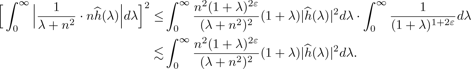 \begin{align*}
\Big[
\int_{0}^\infty
\Big|
\frac{1}{\lambda+n^2}\cdot
n\widehat{h}(\lambda)
\Big|
d\lambda
\Big]^2
\le&
\int_{0}^{\infty}
\frac{n^2(1+\lambda)^{2\varepsilon}}{(\lambda+n^2)^2}
(1+\lambda)|\widehat{h}(\lambda)|^2
d\lambda
\cdot
\int_{0}^{\infty}
\frac{1}{(1+\lambda)^{1+2\varepsilon}}
d\lambda
\\
\lesssim&
\int_{0}^{\infty}
\frac{n^2(1+\lambda)^{2\varepsilon}}{(\lambda+n^2)^2}
(1+\lambda)|\widehat{h}(\lambda)|^2
d\lambda.
\end{align*}
\begin{align*}
\Big[
\int_{0}^\infty
\Big|
\frac{1}{\lambda+n^2}\cdot
n\widehat{h}(\lambda)
\Big|
d\lambda
\Big]^2
\le&
\int_{0}^{\infty}
\frac{n^2(1+\lambda)^{2\varepsilon}}{(\lambda+n^2)^2}
(1+\lambda)|\widehat{h}(\lambda)|^2
d\lambda
\cdot
\int_{0}^{\infty}
\frac{1}{(1+\lambda)^{1+2\varepsilon}}
d\lambda
\\
\lesssim&
\int_{0}^{\infty}
\frac{n^2(1+\lambda)^{2\varepsilon}}{(\lambda+n^2)^2}
(1+\lambda)|\widehat{h}(\lambda)|^2
d\lambda.
\end{align*}Thus, combining above estimates, we get
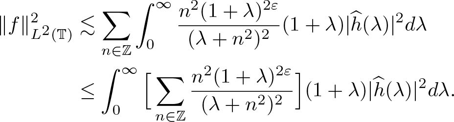 \begin{align*}
\|f\|_{L^2({\mathbb{T}})}^2&
\lesssim
\sum\limits_{n\in{\mathbb Z}}
\int_{0}^{\infty}
\frac{n^2(1+\lambda)^{2\varepsilon}}{(\lambda+n^2)^2}
(1+\lambda)|\widehat{h}(\lambda)|^2
d\lambda
\\&
\le
\int_{0}^{\infty}
\Big[
\sum\limits_{n\in{\mathbb Z}}
\frac{n^2(1+\lambda)^{2\varepsilon}}{(\lambda+n^2)^2}
\Big]
(1+\lambda)|\widehat{h}(\lambda)|^2
d\lambda.
\end{align*}
\begin{align*}
\|f\|_{L^2({\mathbb{T}})}^2&
\lesssim
\sum\limits_{n\in{\mathbb Z}}
\int_{0}^{\infty}
\frac{n^2(1+\lambda)^{2\varepsilon}}{(\lambda+n^2)^2}
(1+\lambda)|\widehat{h}(\lambda)|^2
d\lambda
\\&
\le
\int_{0}^{\infty}
\Big[
\sum\limits_{n\in{\mathbb Z}}
\frac{n^2(1+\lambda)^{2\varepsilon}}{(\lambda+n^2)^2}
\Big]
(1+\lambda)|\widehat{h}(\lambda)|^2
d\lambda.
\end{align*} Furthermore, using  $\lambda+n^2\ge \max\{\lambda, n^2\}$, for all $\lambda\ge 0$ and for $2-2\varepsilon \gt \frac32$ or $\varepsilon \lt \frac14$, we obtain
 \begin{align*}
\sum\limits_{n\in{\mathbb Z}}
\frac{n^2(1+\lambda)^{2\varepsilon}}{(\lambda+n^2)^2}
\le
\sum\limits_{n\in{\mathbb Z}}
\frac{n^2}{(\lambda+n^2)^{2-2\varepsilon}}
\cdot
\frac{(1+\lambda)^{2\varepsilon}}{(\lambda+n^2)^{2\varepsilon}}
\le
\sum\limits_{n\in{\mathbb Z}}
\frac{n^2}{(\lambda+n^2)^{\frac32+}}
\lesssim
\sum\limits_{n=1}^{\infty}
\frac{1}{n^{1+}}
\lesssim 1.
\end{align*}
\begin{align*}
\sum\limits_{n\in{\mathbb Z}}
\frac{n^2(1+\lambda)^{2\varepsilon}}{(\lambda+n^2)^2}
\le
\sum\limits_{n\in{\mathbb Z}}
\frac{n^2}{(\lambda+n^2)^{2-2\varepsilon}}
\cdot
\frac{(1+\lambda)^{2\varepsilon}}{(\lambda+n^2)^{2\varepsilon}}
\le
\sum\limits_{n\in{\mathbb Z}}
\frac{n^2}{(\lambda+n^2)^{\frac32+}}
\lesssim
\sum\limits_{n=1}^{\infty}
\frac{1}{n^{1+}}
\lesssim 1.
\end{align*} Therefore, the desired L 2 estimate (4.43) for  $I_1^{+}$ is reached.
L 4 estimate (4.44) for  $I_1^{+}$. Fubini’s theorem implies
 \begin{align*}
I_1^{+}(r,t)
=&
-
\frac{i\psi(t)}{2\pi}
\int_{0}^\infty
\sum\limits_{n\in{\mathbb Z}}
\frac{ne^{inr}}{\lambda+n^2}
\cdot
e^{i\lambda t}
\widehat{h}(\lambda)
d\lambda
=
-
\frac{i\psi(t)}{2\pi}
\cdot
2i
\int_{0}^\infty
\sum\limits_{n=1}^{\infty}
\frac{n\sin(nr)}{\lambda+n^2}
\\&
\cdot
e^{i\lambda t}
\widehat{h}(\lambda)
d\lambda
\\
=&
\frac{\psi(t)}{\pi}
\int_{0}^\infty
\sum\limits_{n=1}^{\infty}
\frac{n\sin(nr)}{\lambda+n^2}
\cdot
e^{i\lambda t}
\widehat{h}(\lambda)
d\lambda.
\end{align*}
\begin{align*}
I_1^{+}(r,t)
=&
-
\frac{i\psi(t)}{2\pi}
\int_{0}^\infty
\sum\limits_{n\in{\mathbb Z}}
\frac{ne^{inr}}{\lambda+n^2}
\cdot
e^{i\lambda t}
\widehat{h}(\lambda)
d\lambda
=
-
\frac{i\psi(t)}{2\pi}
\cdot
2i
\int_{0}^\infty
\sum\limits_{n=1}^{\infty}
\frac{n\sin(nr)}{\lambda+n^2}
\\&
\cdot
e^{i\lambda t}
\widehat{h}(\lambda)
d\lambda
\\
=&
\frac{\psi(t)}{\pi}
\int_{0}^\infty
\sum\limits_{n=1}^{\infty}
\frac{n\sin(nr)}{\lambda+n^2}
\cdot
e^{i\lambda t}
\widehat{h}(\lambda)
d\lambda.
\end{align*} Since  $\lambda\ge 0$, we see that $\lambda+n^2$ is away from 0 and $\lambda+n^2\ge \max\{\lambda, n^2\}$. Thus, by Cauchy–Schwarz inequality, we have
 \begin{align*}
|I_1^+(r,t)|^2
\lesssim
\psi(t)\sum\limits_{n\in{\mathbb Z}}\int_{0}^\infty \frac{n^2}{|\lambda+n^2|^2(1+\lambda)}
d\lambda
\cdot
\int_{0}^\infty
(1+\lambda)|\widehat{h}(\lambda)|^2d\lambda.
\end{align*}
\begin{align*}
|I_1^+(r,t)|^2
\lesssim
\psi(t)\sum\limits_{n\in{\mathbb Z}}\int_{0}^\infty \frac{n^2}{|\lambda+n^2|^2(1+\lambda)}
d\lambda
\cdot
\int_{0}^\infty
(1+\lambda)|\widehat{h}(\lambda)|^2d\lambda.
\end{align*} Then, for any  $0 \lt \varepsilon \lt \frac12$,
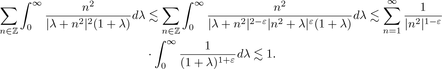 \begin{align*}
\sum\limits_{n\in{\mathbb Z}}\int_{0}^\infty \frac{n^2}{|\lambda+n^2|^2(1+\lambda)}
d\lambda&
\lesssim
\sum\limits_{n\in{\mathbb Z}}\int_{0}^\infty \frac{n^2}{|\lambda+n^2|^{2-\varepsilon}|n^2+\lambda|^{\varepsilon}(1+\lambda)}
d\lambda
\lesssim
\sum\limits_{n=1}^\infty \frac{1}{|n^2|^{1-\varepsilon} }\\&
\cdot
\int_{0}^\infty\frac{1}{(1+\lambda)^{1+\varepsilon}}
d\lambda
\lesssim
1.
\end{align*}
\begin{align*}
\sum\limits_{n\in{\mathbb Z}}\int_{0}^\infty \frac{n^2}{|\lambda+n^2|^2(1+\lambda)}
d\lambda&
\lesssim
\sum\limits_{n\in{\mathbb Z}}\int_{0}^\infty \frac{n^2}{|\lambda+n^2|^{2-\varepsilon}|n^2+\lambda|^{\varepsilon}(1+\lambda)}
d\lambda
\lesssim
\sum\limits_{n=1}^\infty \frac{1}{|n^2|^{1-\varepsilon} }\\&
\cdot
\int_{0}^\infty\frac{1}{(1+\lambda)^{1+\varepsilon}}
d\lambda
\lesssim
1.
\end{align*}Hence, the above estimate yields
 \begin{align*}
|I_1^{+}(r,t)|
\le
\psi(t)
\|h\|_{H^{1/2}},
\quad
-\pi \lt r \lt \pi,
\,\,
t\in{\mathbb R},
\end{align*}
\begin{align*}
|I_1^{+}(r,t)|
\le
\psi(t)
\|h\|_{H^{1/2}},
\quad
-\pi \lt r \lt \pi,
\,\,
t\in{\mathbb R},
\end{align*}which gives
 \begin{equation*}
\|I_1^{+}\|_{L^4({\mathbb{T}}\times {\mathbb R})}
\lesssim
\|h\|_{H^{1/2}}.
\end{equation*}
\begin{equation*}
\|I_1^{+}\|_{L^4({\mathbb{T}}\times {\mathbb R})}
\lesssim
\|h\|_{H^{1/2}}.
\end{equation*} Estimate for  $I_2^{+}$. The L 2 estimate(4.43) for $I_2^{+}$ is similar to the L 2 estimate for $I_1^{+}$ and hence we omit it here. For the L 4 estimate (4.44), taking Fourier transform with respect to r, we have
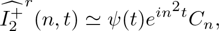 \begin{align*}
\widehat{I_2^+}^r(n,t)
\simeq
\psi(t)e^{in^2 t}C_n,
\end{align*}
\begin{align*}
\widehat{I_2^+}^r(n,t)
\simeq
\psi(t)e^{in^2 t}C_n,
\end{align*}where
 \begin{align*}
C_n
=
\int_{0}^{\infty}
\frac{n}{\lambda+n^2}\widehat{h}(\lambda)d\lambda.
\end{align*}
\begin{align*}
C_n
=
\int_{0}^{\infty}
\frac{n}{\lambda+n^2}\widehat{h}(\lambda)d\lambda.
\end{align*} Then, the Fourier transform of  $\widehat f^r$ with respect to t gives
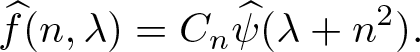 \begin{align*}
\widehat f(n,\lambda)
=
C_n\widehat \psi(\lambda+n^2).
\end{align*}
\begin{align*}
\widehat f(n,\lambda)
=
C_n\widehat \psi(\lambda+n^2).
\end{align*}Applying (4.17) yields
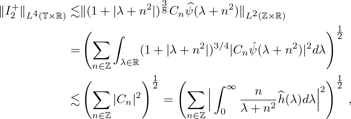 \begin{align}
\|I_2^{+}\|_{L^4({\mathbb{T}}\times {\mathbb R})}
\lesssim&
\|(1+|\lambda+n^2|)^{\frac{3}{8}}
C_n\widehat \psi(\lambda+n^2)
\|_{L^2({\mathbb Z}\times{\mathbb R})}
\nonumber
\\
=&
\left(
\sum\limits_{n\in{\mathbb Z}}
\int_{\lambda\in{\mathbb R}}
(1+|\lambda+n^2|)^{3/4}
|C_n\hat \psi(\lambda+n^2)|^2d\lambda
\right)^\frac12
\nonumber
\\
\lesssim&
\left(
\sum\limits_{n\in{\mathbb Z}}
|C_n|^2
\right)^\frac12
=
\left(
\sum\limits_{n\in{\mathbb Z}}
\Big|
\int_0^{\infty}
\frac{n}{\lambda+n^2}\widehat{h}(\lambda)d\lambda
\Big|^2
\right)^\frac12 \, ,
\end{align}
\begin{align}
\|I_2^{+}\|_{L^4({\mathbb{T}}\times {\mathbb R})}
\lesssim&
\|(1+|\lambda+n^2|)^{\frac{3}{8}}
C_n\widehat \psi(\lambda+n^2)
\|_{L^2({\mathbb Z}\times{\mathbb R})}
\nonumber
\\
=&
\left(
\sum\limits_{n\in{\mathbb Z}}
\int_{\lambda\in{\mathbb R}}
(1+|\lambda+n^2|)^{3/4}
|C_n\hat \psi(\lambda+n^2)|^2d\lambda
\right)^\frac12
\nonumber
\\
\lesssim&
\left(
\sum\limits_{n\in{\mathbb Z}}
|C_n|^2
\right)^\frac12
=
\left(
\sum\limits_{n\in{\mathbb Z}}
\Big|
\int_0^{\infty}
\frac{n}{\lambda+n^2}\widehat{h}(\lambda)d\lambda
\Big|^2
\right)^\frac12 \, ,
\end{align} which reduces to the estimate (4.51). We complete the estimates for  $I_2^{+}$.
Estimate for  $I^-$. Adding and subtracting $\psi(\lambda+n^2)$ inside the integral (localizing near the singularity $\lambda=-n^2$) gives the following decomposition of $I^-$,
 \begin{align}
I^-
=&
-
\frac{i\psi(t)}{2\pi}
\sum\limits_{n\in{\mathbb Z}}\int_{-\infty}^{0}
e^{inr}e^{i\lambda t}
\frac{1-\psi(\lambda+n^2)}{\lambda+n^2}\cdot
n\widehat{h}(\lambda)
d\lambda
\end{align}
\begin{align}
I^-
=&
-
\frac{i\psi(t)}{2\pi}
\sum\limits_{n\in{\mathbb Z}}\int_{-\infty}^{0}
e^{inr}e^{i\lambda t}
\frac{1-\psi(\lambda+n^2)}{\lambda+n^2}\cdot
n\widehat{h}(\lambda)
d\lambda
\end{align} \begin{align}
&+
\frac{i\psi(t)}{2\pi}
\sum\limits_{n\in{\mathbb Z}}\int_{-\infty}^{0} e^{inr}e^{-in^2t}\frac{1-\psi(\lambda+n^2)}{\lambda+n^2}\cdot
n\widehat{h}(\lambda)
d\lambda
\end{align}
\begin{align}
&+
\frac{i\psi(t)}{2\pi}
\sum\limits_{n\in{\mathbb Z}}\int_{-\infty}^{0} e^{inr}e^{-in^2t}\frac{1-\psi(\lambda+n^2)}{\lambda+n^2}\cdot
n\widehat{h}(\lambda)
d\lambda
\end{align}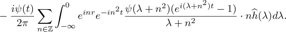 \begin{align}
&-
\frac{i\psi(t)}{2\pi}\sum\limits_{n\in{\mathbb Z}}\int_{-\infty}^{0} e^{inr}e^{-in^2t}\frac{\psi(\lambda+n^2)(e^{i(\lambda+n^2)t}-1)}{\lambda+n^2}\cdot
n\widehat{h}(\lambda)
d\lambda.
\end{align}
\begin{align}
&-
\frac{i\psi(t)}{2\pi}\sum\limits_{n\in{\mathbb Z}}\int_{-\infty}^{0} e^{inr}e^{-in^2t}\frac{\psi(\lambda+n^2)(e^{i(\lambda+n^2)t}-1)}{\lambda+n^2}\cdot
n\widehat{h}(\lambda)
d\lambda.
\end{align}Estimates for (4.53). First, we prove (4.43) for this term. Let
 \begin{equation*}
f(r,t)
=
\sum\limits_{n\in{\mathbb Z}}
e^{inr}
\int_{-\infty}^{0}
e^{i\lambda t}
\frac{1-\psi(\lambda+n^2)}{\lambda+n^2}\cdot
n\widehat{h}(\lambda)
d\lambda\, .
\end{equation*}
\begin{equation*}
f(r,t)
=
\sum\limits_{n\in{\mathbb Z}}
e^{inr}
\int_{-\infty}^{0}
e^{i\lambda t}
\frac{1-\psi(\lambda+n^2)}{\lambda+n^2}\cdot
n\widehat{h}(\lambda)
d\lambda\, .
\end{equation*} Since ψ is compactly supported in  $(0,1)$, we have $\sup\limits_{t\in[0,T]}\|(4.53)\|_{L^2({\mathbb{T}})}\le \sup\limits_{t\in[0,1]}\|f\|_{L^2({\mathbb{T}})}$. Taking the Fourier transform of f with respect to r gives
 \begin{equation}
\widehat{f}^r
(n,t)
\simeq
\int_{-\infty}^{0}
e^{i\lambda t}
\frac{1-\psi(\lambda+n^2)}{\lambda+n^2}\cdot
n\widehat{h}(\lambda)
d\lambda,
\end{equation}
\begin{equation}
\widehat{f}^r
(n,t)
\simeq
\int_{-\infty}^{0}
e^{i\lambda t}
\frac{1-\psi(\lambda+n^2)}{\lambda+n^2}\cdot
n\widehat{h}(\lambda)
d\lambda,
\end{equation}which implies that
 \begin{align}
\|f\|_{L^2({\mathbb{T}})}^2&
\lesssim
\sum\limits_{n\in{\mathbb Z}}
\Big|
\int_{-\infty}^{0}
e^{i\lambda t}
\frac{1-\psi(\lambda+n^2)}{\lambda+n^2}\cdot
n\widehat{h}(\lambda)
d\lambda
\Big|^2\\&
\le
\sum\limits_{n\in{\mathbb Z}}
\Big[
\int_{-\infty}^{0}
\Big|
\frac{1-\psi(\lambda+n^2)}{\lambda+n^2}\cdot
n\widehat{h}(\lambda)
\Big|
d\lambda
\Big]^2.
\end{align}
\begin{align}
\|f\|_{L^2({\mathbb{T}})}^2&
\lesssim
\sum\limits_{n\in{\mathbb Z}}
\Big|
\int_{-\infty}^{0}
e^{i\lambda t}
\frac{1-\psi(\lambda+n^2)}{\lambda+n^2}\cdot
n\widehat{h}(\lambda)
d\lambda
\Big|^2\\&
\le
\sum\limits_{n\in{\mathbb Z}}
\Big[
\int_{-\infty}^{0}
\Big|
\frac{1-\psi(\lambda+n^2)}{\lambda+n^2}\cdot
n\widehat{h}(\lambda)
\Big|
d\lambda
\Big]^2.
\end{align} Also, making the change of variables  $\lambda=-\mu^2$ and using $\frac{n}{n^2-\mu^2}=\frac12\big[\frac{1}{n-\mu}+\frac{1}{n+\mu}\big]$, it is deduced that
 \begin{align*}
\|f\|_{L^2({\mathbb{T}})}^2
\lesssim
\sum\limits_{n\in{\mathbb Z}}
\Big[
\int_{0}^{\infty}
|
\mu
\widehat{h}(-\mu^2)
|
|\frac{1}{n-\mu}+\frac{1}{n+\mu}|
[1-\psi(n^2-\mu^2)]
d\lambda
\Big]^2.
\end{align*}
\begin{align*}
\|f\|_{L^2({\mathbb{T}})}^2
\lesssim
\sum\limits_{n\in{\mathbb Z}}
\Big[
\int_{0}^{\infty}
|
\mu
\widehat{h}(-\mu^2)
|
|\frac{1}{n-\mu}+\frac{1}{n+\mu}|
[1-\psi(n^2-\mu^2)]
d\lambda
\Big]^2.
\end{align*}Now we need the following estimate, whose proof is provided in [Reference Bona, Sun and Zhang7],
 \begin{align*}
\sum\limits_{n\in{\mathbb Z}}
\Big|
\int_0^\infty
\widehat{F}(\mu)
\frac{1}{n-\mu}
(1-\psi(n^2-\mu^2))
d\mu
\Big|^2
\lesssim
\int_0^\infty
(1+\mu)|\widehat{F}(\mu)|^2
d\mu.
\end{align*}
\begin{align*}
\sum\limits_{n\in{\mathbb Z}}
\Big|
\int_0^\infty
\widehat{F}(\mu)
\frac{1}{n-\mu}
(1-\psi(n^2-\mu^2))
d\mu
\Big|^2
\lesssim
\int_0^\infty
(1+\mu)|\widehat{F}(\mu)|^2
d\mu.
\end{align*} In fact, applying the above estimate twice with  $\widehat{F}(\mu)=|
\mu
\widehat{h}(-\mu^2)
|$ implies
$\widehat{F}(\mu)=|
\mu
\widehat{h}(-\mu^2)
|$ implies
 \begin{align*}
\|f\|_{L^2({\mathbb{T}})}^2
\lesssim
\int_0^\infty
(1+\mu)|\mu\widehat{h}(\mu^2)|^2
d\mu
\lesssim
\int_{\mathbb R}
(1+|\lambda|^{1/2})
|\lambda|^{1/2}
|\widehat{h}(\lambda)|^2
d\lambda
\lesssim
\|h\|_{H^{1/2}}^2.
\end{align*}
\begin{align*}
\|f\|_{L^2({\mathbb{T}})}^2
\lesssim
\int_0^\infty
(1+\mu)|\mu\widehat{h}(\mu^2)|^2
d\mu
\lesssim
\int_{\mathbb R}
(1+|\lambda|^{1/2})
|\lambda|^{1/2}
|\widehat{h}(\lambda)|^2
d\lambda
\lesssim
\|h\|_{H^{1/2}}^2.
\end{align*} L 4 estimate (4.44) for (4.53). To show this estimate, we will split the  $d\lambda$-integral at $\lambda=-\frac{n^2}{2}$. More precisely, we have
 \begin{align*}
(4.53)
=
-
\frac{i\psi(t)}{2\pi}
f_1
-
\frac{i\psi(t)}{2\pi}
f_2,
\end{align*}
\begin{align*}
(4.53)
=
-
\frac{i\psi(t)}{2\pi}
f_1
-
\frac{i\psi(t)}{2\pi}
f_2,
\end{align*}where
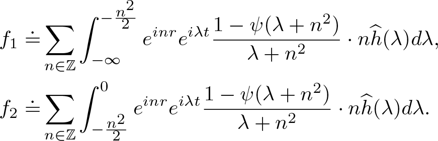 \begin{align*}
f_1
\doteq&
\sum\limits_{n\in{\mathbb Z}}\int_{-\infty}^{-\frac{n^2}{2}}
e^{inr}e^{i\lambda t}
\frac{1-\psi(\lambda+n^2)}{\lambda+n^2}\cdot
n\widehat{h}(\lambda)
d\lambda,
\\
f_2
\doteq&
\sum\limits_{n\in{\mathbb Z}}\int_{-\frac{n^2}{2}}^{0}
e^{inr}e^{i\lambda t}
\frac{1-\psi(\lambda+n^2)}{\lambda+n^2}\cdot
n\widehat{h}(\lambda)
d\lambda.
\end{align*}
\begin{align*}
f_1
\doteq&
\sum\limits_{n\in{\mathbb Z}}\int_{-\infty}^{-\frac{n^2}{2}}
e^{inr}e^{i\lambda t}
\frac{1-\psi(\lambda+n^2)}{\lambda+n^2}\cdot
n\widehat{h}(\lambda)
d\lambda,
\\
f_2
\doteq&
\sum\limits_{n\in{\mathbb Z}}\int_{-\frac{n^2}{2}}^{0}
e^{inr}e^{i\lambda t}
\frac{1-\psi(\lambda+n^2)}{\lambda+n^2}\cdot
n\widehat{h}(\lambda)
d\lambda.
\end{align*} For  $\frac{i\psi(t)}{2\pi}
f_1$, since ψ is compactly supported in
$\frac{i\psi(t)}{2\pi}
f_1$, since ψ is compactly supported in  $(0,1)$, we have
  $\|\frac{i\psi(t)}{2\pi}
f_1\|_{L^4({\mathbb{T}}\times{\mathbb R})}\lesssim \|f_1\|_{L^4({\mathbb{T}}\times{\mathbb R})}$. Also, we have
$\|\frac{i\psi(t)}{2\pi}
f_1\|_{L^4({\mathbb{T}}\times{\mathbb R})}\lesssim \|f_1\|_{L^4({\mathbb{T}}\times{\mathbb R})}$. Also, we have  $|n|^2\lesssim |\lambda|$. Thus, applying estimate (4.17) gives
 \begin{align*}
\|f_1\|_{L^4({\mathbb{T}}\times{\mathbb R})}^2
\lesssim&
\sum\limits_{n\in{\mathbb Z}}
\int_{\mathbb R}
(1+|\lambda+n^2|)^{\frac{3}{4}}
\chi_{\lambda \lt -\frac{n^2}{2}}(\lambda)
\Big|
\frac{1-\psi(\lambda+n^2)}{\lambda+n^2}\cdot
n\widehat{h}(\lambda)
\Big|^2
d\lambda
\\
\lesssim&
\sum\limits_{n\in{\mathbb Z}}
\int_{\mathbb R}
\frac{1}{(1+|\lambda+n^2|)^{5/4}}\cdot
|\lambda|
|\widehat{h}(\lambda)
|^2
d\lambda
\\
\lesssim&
\int_{\mathbb R}
\sum\limits_{n\in{\mathbb Z}}
\frac{1}{(1+|\lambda+n^2|)^{5/4}}\cdot
|\lambda|
|\widehat{h}(\lambda)
|^2
d\lambda
\\
\lesssim&
\int_{\mathbb R}
|\lambda|
|\widehat{h}(\lambda)
|^2
d\lambda
\lesssim
\|h\|_{H^{1/2}}.
\end{align*}
\begin{align*}
\|f_1\|_{L^4({\mathbb{T}}\times{\mathbb R})}^2
\lesssim&
\sum\limits_{n\in{\mathbb Z}}
\int_{\mathbb R}
(1+|\lambda+n^2|)^{\frac{3}{4}}
\chi_{\lambda \lt -\frac{n^2}{2}}(\lambda)
\Big|
\frac{1-\psi(\lambda+n^2)}{\lambda+n^2}\cdot
n\widehat{h}(\lambda)
\Big|^2
d\lambda
\\
\lesssim&
\sum\limits_{n\in{\mathbb Z}}
\int_{\mathbb R}
\frac{1}{(1+|\lambda+n^2|)^{5/4}}\cdot
|\lambda|
|\widehat{h}(\lambda)
|^2
d\lambda
\\
\lesssim&
\int_{\mathbb R}
\sum\limits_{n\in{\mathbb Z}}
\frac{1}{(1+|\lambda+n^2|)^{5/4}}\cdot
|\lambda|
|\widehat{h}(\lambda)
|^2
d\lambda
\\
\lesssim&
\int_{\mathbb R}
|\lambda|
|\widehat{h}(\lambda)
|^2
d\lambda
\lesssim
\|h\|_{H^{1/2}}.
\end{align*} For  $\frac{i\psi(t)}{2\pi}
f_2$, again since
$\frac{i\psi(t)}{2\pi}
f_2$, again since  $\psi(t)$ is compactly supported in $(0,1)$, it suffices to show that
 \begin{align}
\|f_2\|_{L^\infty_{{\mathbb{T}}\times{\mathbb R}}}
\lesssim
\|h\|_{H^{1/2}}.
\end{align}
\begin{align}
\|f_2\|_{L^\infty_{{\mathbb{T}}\times{\mathbb R}}}
\lesssim
\|h\|_{H^{1/2}}.
\end{align}By Cauchy–Schwarz inequality,
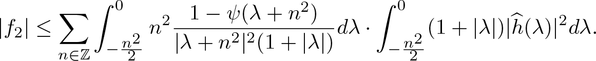 \begin{align*}
|f_2|
\le
\sum\limits_{n\in{\mathbb Z}}\int_{-\frac{n^2}{2}}^{0}
n^2
\frac{1-\psi(\lambda+n^2)}{|\lambda+n^2|^2(1+|\lambda|)}
d\lambda
\cdot
\int_{-\frac{n^2}{2}}^{0}
(1+|\lambda|)
|\widehat{h}(\lambda)|^2
d\lambda.
\end{align*}
\begin{align*}
|f_2|
\le
\sum\limits_{n\in{\mathbb Z}}\int_{-\frac{n^2}{2}}^{0}
n^2
\frac{1-\psi(\lambda+n^2)}{|\lambda+n^2|^2(1+|\lambda|)}
d\lambda
\cdot
\int_{-\frac{n^2}{2}}^{0}
(1+|\lambda|)
|\widehat{h}(\lambda)|^2
d\lambda.
\end{align*} For the first integral in the above estimate, choosing  $0 \lt \varepsilon \lt \frac12$, we have
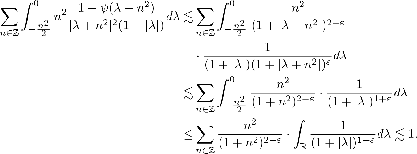 \begin{align*}
\sum\limits_{n\in{\mathbb Z}}\int_{-\frac{n^2}{2}}^{0}
n^2
\frac{1-\psi(\lambda+n^2)}{|\lambda+n^2|^2(1+|\lambda|)}
d\lambda
\lesssim&
\sum\limits_{n\in{\mathbb Z}}\int_{-\frac{n^2}{2}}^{0}
\frac{n^2}{(1+|\lambda+n^2|)^{2-\varepsilon}}\\&
\cdot
\frac{1}{(1+|\lambda|)(1+|\lambda+n^2|)^{\varepsilon}}
d\lambda
\\
\lesssim&
\sum\limits_{n\in{\mathbb Z}}\int_{-\frac{n^2}{2}}^{0}
\frac{n^2}{(1+n^2)^{2-\varepsilon}}
\cdot
\frac{1}{(1+|\lambda|)^{1+\varepsilon}}
d\lambda
\\
\le &
\sum\limits_{n\in{\mathbb Z}}
\frac{n^2}{(1+n^2)^{2-\varepsilon}}
\cdot
\int_{{\mathbb R}}
\frac{1}{(1+|\lambda|)^{1+\varepsilon}}
d\lambda
\lesssim
1.
\end{align*}
\begin{align*}
\sum\limits_{n\in{\mathbb Z}}\int_{-\frac{n^2}{2}}^{0}
n^2
\frac{1-\psi(\lambda+n^2)}{|\lambda+n^2|^2(1+|\lambda|)}
d\lambda
\lesssim&
\sum\limits_{n\in{\mathbb Z}}\int_{-\frac{n^2}{2}}^{0}
\frac{n^2}{(1+|\lambda+n^2|)^{2-\varepsilon}}\\&
\cdot
\frac{1}{(1+|\lambda|)(1+|\lambda+n^2|)^{\varepsilon}}
d\lambda
\\
\lesssim&
\sum\limits_{n\in{\mathbb Z}}\int_{-\frac{n^2}{2}}^{0}
\frac{n^2}{(1+n^2)^{2-\varepsilon}}
\cdot
\frac{1}{(1+|\lambda|)^{1+\varepsilon}}
d\lambda
\\
\le &
\sum\limits_{n\in{\mathbb Z}}
\frac{n^2}{(1+n^2)^{2-\varepsilon}}
\cdot
\int_{{\mathbb R}}
\frac{1}{(1+|\lambda|)^{1+\varepsilon}}
d\lambda
\lesssim
1.
\end{align*}Combining the above estimates yields the desired estimate (4.58).
Estimates for (4.54). We let
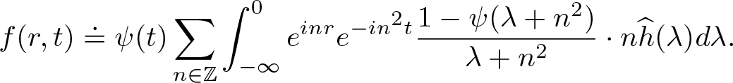 \begin{align*}
f(r,t)
\doteq
\psi(t)
\sum\limits_{n\in{\mathbb Z}}\int_{-\infty}^{0} e^{inr}e^{-in^2t}\frac{1-\psi(\lambda+n^2)}{\lambda+n^2}\cdot
n\widehat{h}(\lambda)
d\lambda.
\end{align*}
\begin{align*}
f(r,t)
\doteq
\psi(t)
\sum\limits_{n\in{\mathbb Z}}\int_{-\infty}^{0} e^{inr}e^{-in^2t}\frac{1-\psi(\lambda+n^2)}{\lambda+n^2}\cdot
n\widehat{h}(\lambda)
d\lambda.
\end{align*}Taking Fourier transform with respect to r, it is obtained that
 \begin{align*}
\widehat{f}^r(n,t)
\simeq
\psi(t)e^{-in^2 t}C_n,
\end{align*}
\begin{align*}
\widehat{f}^r(n,t)
\simeq
\psi(t)e^{-in^2 t}C_n,
\end{align*}where
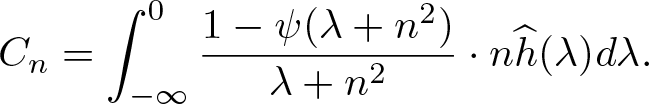 \begin{align*}
C_n
=
\int_{-\infty}^{0}
\frac{1-\psi(\lambda+n^2)}{\lambda+n^2}\cdot
n\widehat{h}(\lambda)d\lambda.
\end{align*}
\begin{align*}
C_n
=
\int_{-\infty}^{0}
\frac{1-\psi(\lambda+n^2)}{\lambda+n^2}\cdot
n\widehat{h}(\lambda)d\lambda.
\end{align*}Hence, by Plancherel’s theorem, we have
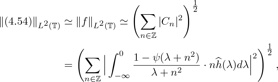 \begin{align*}
\|(4.54)\|_{L^2({\mathbb{T}})}&
\simeq
\|f\|_{L^2({\mathbb{T}})}
\simeq
\left(
\sum\limits_{n\in{\mathbb Z}}
|C_n|^2
\right)^\frac12\\&
=
\left(
\sum\limits_{n\in{\mathbb Z}}
\Big|
\int_{-\infty}^{0}
\frac{1-\psi(\lambda+n^2)}{\lambda+n^2}\cdot
n\widehat{h}(\lambda)d\lambda
\Big|^2
\right)^\frac12,
\end{align*}
\begin{align*}
\|(4.54)\|_{L^2({\mathbb{T}})}&
\simeq
\|f\|_{L^2({\mathbb{T}})}
\simeq
\left(
\sum\limits_{n\in{\mathbb Z}}
|C_n|^2
\right)^\frac12\\&
=
\left(
\sum\limits_{n\in{\mathbb Z}}
\Big|
\int_{-\infty}^{0}
\frac{1-\psi(\lambda+n^2)}{\lambda+n^2}\cdot
n\widehat{h}(\lambda)d\lambda
\Big|^2
\right)^\frac12,
\end{align*} which is reduced to the estimate (4.57). Concerning L 4 estimate of (4.54), computing the Fourier transform of  $\widehat f^r$ with respect to t gives
 \begin{align*}
\widehat f(n,\lambda)
=
C_n\widehat \psi(\lambda+n^2).
\end{align*}
\begin{align*}
\widehat f(n,\lambda)
=
C_n\widehat \psi(\lambda+n^2).
\end{align*} Estimate (4.17) gives  $
\|I_2^{+}\|_{L^4({\mathbb{T}}\times {\mathbb R})}
\lesssim
\|(1+|\lambda+n^2|)^{\frac{3}{8}}
C_n\widehat \psi(\lambda+n^2)
\|_{L^2({\mathbb Z}\times{\mathbb R})}.
$ This implies
$
\|I_2^{+}\|_{L^4({\mathbb{T}}\times {\mathbb R})}
\lesssim
\|(1+|\lambda+n^2|)^{\frac{3}{8}}
C_n\widehat \psi(\lambda+n^2)
\|_{L^2({\mathbb Z}\times{\mathbb R})}.
$ This implies
 \begin{align*}
\|I_2^{+}\|_{L^4({\mathbb{T}}\times {\mathbb R})}
\lesssim
\left(
\sum\limits_{n\in{\mathbb Z}}
\int_{\lambda\in{\mathbb R}}
(1+|\lambda+n^2|)^{3/4}
|C_n\hat \psi(\lambda+n^2)|^2d\lambda
\right)^\frac12
\lesssim
\left(
\sum\limits_{n\in{\mathbb Z}}
|C_n|^2
\right)^\frac12.
\end{align*}
\begin{align*}
\|I_2^{+}\|_{L^4({\mathbb{T}}\times {\mathbb R})}
\lesssim
\left(
\sum\limits_{n\in{\mathbb Z}}
\int_{\lambda\in{\mathbb R}}
(1+|\lambda+n^2|)^{3/4}
|C_n\hat \psi(\lambda+n^2)|^2d\lambda
\right)^\frac12
\lesssim
\left(
\sum\limits_{n\in{\mathbb Z}}
|C_n|^2
\right)^\frac12.
\end{align*}Again, we arrive at estimate (4.57). This completes L 4 estimate of (4.54).
Estimates for (4.55). Using Taylor’s series at  $\lambda+n^2=0$, we obtain
 \begin{equation*}
e^{i(\lambda+n^2)t}-1
=
\sum\limits_{k=1}^\infty
\frac{(it)^k(\lambda+n^2)^k}{k!}.
\end{equation*}
\begin{equation*}
e^{i(\lambda+n^2)t}-1
=
\sum\limits_{k=1}^\infty
\frac{(it)^k(\lambda+n^2)^k}{k!}.
\end{equation*} Thus,  $(4.55)\simeq\sum\limits_{k=1}^\infty \frac{i^{k+1}}{k!}f_k$, where
 \begin{align*}
f_k(r,t)
\doteq
t^k \psi(t)
\sum\limits_{n\in{\mathbb Z}}\int_{-\infty}^0
e^{inr}e^{-in^2t}
\psi(\lambda+n^2)(\lambda+n^2)^{k-1}
n
\widehat{h}(\lambda) d\lambda.
\end{align*}
\begin{align*}
f_k(r,t)
\doteq
t^k \psi(t)
\sum\limits_{n\in{\mathbb Z}}\int_{-\infty}^0
e^{inr}e^{-in^2t}
\psi(\lambda+n^2)(\lambda+n^2)^{k-1}
n
\widehat{h}(\lambda) d\lambda.
\end{align*}For the L 2 estimate of (4.55), we have
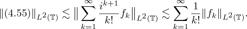 \begin{align*}
\|(4.55)\|_{L^2({\mathbb{T}})}
\lesssim
\big\|
\sum\limits_{k=1}^\infty \frac{i^{k+1}}{k!}f_k
\big\|_{L^2({\mathbb{T}})}
\lesssim
\sum\limits_{k=1}^\infty
\frac{1}{k!}
\|f_k\|_{L^2({\mathbb{T}})}.
\end{align*}
\begin{align*}
\|(4.55)\|_{L^2({\mathbb{T}})}
\lesssim
\big\|
\sum\limits_{k=1}^\infty \frac{i^{k+1}}{k!}f_k
\big\|_{L^2({\mathbb{T}})}
\lesssim
\sum\limits_{k=1}^\infty
\frac{1}{k!}
\|f_k\|_{L^2({\mathbb{T}})}.
\end{align*}Taking the Fourier transform of the function fk, it is deduced that
 \begin{align*}
\widehat f^r_k(n,t)
=
C_k(n)t^k\psi(t)e^{-in^2t},
\end{align*}
\begin{align*}
\widehat f^r_k(n,t)
=
C_k(n)t^k\psi(t)e^{-in^2t},
\end{align*}where
 \begin{align*}
C_k(n)
=
\int_{-\infty}^0
\psi(\lambda+n^2)(\lambda +n^2)^{k-1}
n
\widehat{h}(\lambda) d\lambda.
\end{align*}
\begin{align*}
C_k(n)
=
\int_{-\infty}^0
\psi(\lambda+n^2)(\lambda +n^2)^{k-1}
n
\widehat{h}(\lambda) d\lambda.
\end{align*} Since ψ is compactly supported in  $(0,1)$, by the Plancherel theorem and Cauchy–Schwarz inequality, it is obtained that
 \begin{align*}
\|f_k(t)\|_{L^2({\mathbb{T}})}^2
\lesssim&
\sum\limits_{n\in{\mathbb Z}}
|C_k(n)|^2
=
\Big|
\int_{-\infty}^0
\psi(\lambda+n^2)(\lambda +n^2)^{k-1}
n
\widehat{h}(\lambda) d\lambda
\Big|^2
\\
\lesssim&
\int_{-\infty}^0
\psi(\lambda+n^2)(\lambda +n^2)^{2(k-1)}
d\lambda
\cdot
\int_{-\infty}^0
\psi(\lambda+n^2)
n^2
|\widehat{h}(\lambda)|^2 d\lambda\, .
\end{align*}
\begin{align*}
\|f_k(t)\|_{L^2({\mathbb{T}})}^2
\lesssim&
\sum\limits_{n\in{\mathbb Z}}
|C_k(n)|^2
=
\Big|
\int_{-\infty}^0
\psi(\lambda+n^2)(\lambda +n^2)^{k-1}
n
\widehat{h}(\lambda) d\lambda
\Big|^2
\\
\lesssim&
\int_{-\infty}^0
\psi(\lambda+n^2)(\lambda +n^2)^{2(k-1)}
d\lambda
\cdot
\int_{-\infty}^0
\psi(\lambda+n^2)
n^2
|\widehat{h}(\lambda)|^2 d\lambda\, .
\end{align*} Since  $\psi\in C^\infty_0(0,1)$, the first integral is bounded. Also, for the second integral, $|\lambda+n^2| \lt 1$, which implies that $n^2\lesssim (1+|\lambda|)$. Hence,
 \begin{align*}
\|f_k(t)\|_{L^2({\mathbb{T}})}^2
\lesssim
\int_{-\infty}^0
(1+|\lambda|)
|\widehat{h}(\lambda)|^2 d\lambda
\lesssim
\|h\|_{H^{1/2}}^2.
\end{align*}
\begin{align*}
\|f_k(t)\|_{L^2({\mathbb{T}})}^2
\lesssim
\int_{-\infty}^0
(1+|\lambda|)
|\widehat{h}(\lambda)|^2 d\lambda
\lesssim
\|h\|_{H^{1/2}}^2.
\end{align*}For the L 4 estimate of (4.55), we have
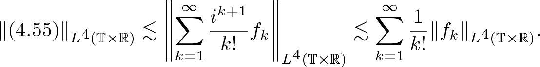 \begin{align*}
\|(4.55)\|_{L^4({\mathbb{T}}\times{\mathbb R})}
\lesssim
\left \|
\sum\limits_{k=1}^\infty \frac{i^{k+1}}{k!}f_k
\right \|_{L^4({\mathbb{T}}\times{\mathbb R})}
\lesssim
\sum\limits_{k=1}^\infty
\frac{1}{k!}
\|f_k\|_{L^4({\mathbb{T}}\times{\mathbb R})}.
\end{align*}
\begin{align*}
\|(4.55)\|_{L^4({\mathbb{T}}\times{\mathbb R})}
\lesssim
\left \|
\sum\limits_{k=1}^\infty \frac{i^{k+1}}{k!}f_k
\right \|_{L^4({\mathbb{T}}\times{\mathbb R})}
\lesssim
\sum\limits_{k=1}^\infty
\frac{1}{k!}
\|f_k\|_{L^4({\mathbb{T}}\times{\mathbb R})}.
\end{align*}To bound the L 4 norm of fk, taking the full Fourier transform, we obtain
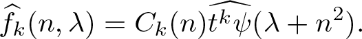 \begin{align*}
\widehat f_k(n,\lambda)
=
C_k(n)\widehat{t^k\psi}(\lambda+n^2).
\end{align*}
\begin{align*}
\widehat f_k(n,\lambda)
=
C_k(n)\widehat{t^k\psi}(\lambda+n^2).
\end{align*}Applying estimate (4.17) gives
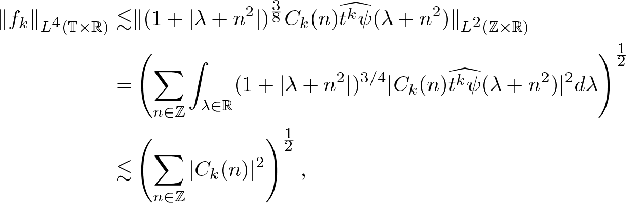 \begin{align*}
\|f_k\|_{L^4({\mathbb{T}}\times {\mathbb R})}
\lesssim&
\|(1+|\lambda+n^2|)^{\frac{3}{8}}
C_k(n)\widehat{t^k \psi}(\lambda+n^2)
\|_{L^2({\mathbb Z}\times{\mathbb R})}
\nonumber
\\
=&
\left(
\sum\limits_{n\in{\mathbb Z}}
\int_{\lambda\in{\mathbb R}}
(1+|\lambda+n^2|)^{3/4}
|C_k(n)\widehat{t^k \psi}(\lambda+n^2)|^2d\lambda
\right)^\frac12\\
\lesssim &
\left(
\sum\limits_{n\in{\mathbb Z}}
|C_k(n)|^2
\right)^\frac12,
\end{align*}
\begin{align*}
\|f_k\|_{L^4({\mathbb{T}}\times {\mathbb R})}
\lesssim&
\|(1+|\lambda+n^2|)^{\frac{3}{8}}
C_k(n)\widehat{t^k \psi}(\lambda+n^2)
\|_{L^2({\mathbb Z}\times{\mathbb R})}
\nonumber
\\
=&
\left(
\sum\limits_{n\in{\mathbb Z}}
\int_{\lambda\in{\mathbb R}}
(1+|\lambda+n^2|)^{3/4}
|C_k(n)\widehat{t^k \psi}(\lambda+n^2)|^2d\lambda
\right)^\frac12\\
\lesssim &
\left(
\sum\limits_{n\in{\mathbb Z}}
|C_k(n)|^2
\right)^\frac12,
\end{align*}which is the estimate needed. This completes the proof of proposition 4.6.
Now, we can derive linear estimate for the solution to the linear ibvp (4.2). In fact, for  $0 \lt r \lt \pi$ and $0 \lt t \lt T$, this solution is given by
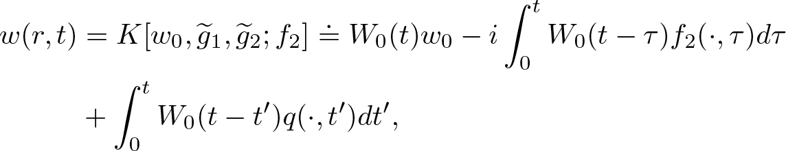 \begin{align}
w(r,t)&
=
K[w_0, \widetilde{g}_1,\widetilde{g}_2; f_2]
\doteq
W_0(t)w_0
-i
\int_0^t
W_0(t-\tau)
f_2(\cdot,\tau)
d\tau\\&
+
\int_0^t W_0(t-t')q(\cdot, t')dt',
\end{align}
\begin{align}
w(r,t)&
=
K[w_0, \widetilde{g}_1,\widetilde{g}_2; f_2]
\doteq
W_0(t)w_0
-i
\int_0^t
W_0(t-\tau)
f_2(\cdot,\tau)
d\tau\\&
+
\int_0^t W_0(t-t')q(\cdot, t')dt',
\end{align} where W 0 is defined by (4.12) and q is given by (4.40) with  $h_1(t)=\widetilde{g}_1(t)$, $h_2(t)=\widetilde{g}_2(t)$. Combining propositions 4.1, 4.3, and 4.6, the following linear estimate holds for solution formula $K[w_0, \widetilde{g}_1,\widetilde{g}_2; f_2]$.
Theorem 4.7 (1) Let  $s\in{\mathbb{N}}$. If $w_0\in H^s(0,\pi)$, $\widetilde{g}_1, \widetilde{g}_2\in H^{\frac{s+1}{2}}_{0}(0,T)$ (for even s, $\widetilde{g}_1, \widetilde{g}_2\in H^{\frac{s+1}{2}}_{00}(0,T)$), and $\partial_r^s f_2\in L^{4/3}\big((0,\pi)\times(0,T)\big)$, then $K[w_0, \widetilde{g}_1,\widetilde{g}_2; f_2]$ defines a solution to the ibvp (4.2), which satisfies
 \begin{align}
&
\sup\limits_{t\in[0,T]}\big\|K[w_0, \widetilde{g}_1,\widetilde{g}_2; f_2](t)\big\|_{H^s(0,\pi)}
+
\big\|
\partial_r^s
K[w_0, \widetilde{g}_1,\widetilde{g}_2; f_2]
\big\|_{L^4((0,\pi)\times(0,T))}
\nonumber
\\
& \qquad \lesssim
\|\omega_0\|_{H^s(0,\pi)}
+
\|\widetilde{g}_1\|_{H^{\frac{s+1}{2}}(0,T)}
+
\|\widetilde{g}_2\|_{H^{\frac{s+1}{2}}(0,T)}
+
\|\partial_r^s f_2\|_{L^{4/3}\big((0,\pi)\times(0,T)\big)}.
\end{align}
\begin{align}
&
\sup\limits_{t\in[0,T]}\big\|K[w_0, \widetilde{g}_1,\widetilde{g}_2; f_2](t)\big\|_{H^s(0,\pi)}
+
\big\|
\partial_r^s
K[w_0, \widetilde{g}_1,\widetilde{g}_2; f_2]
\big\|_{L^4((0,\pi)\times(0,T))}
\nonumber
\\
& \qquad \lesssim
\|\omega_0\|_{H^s(0,\pi)}
+
\|\widetilde{g}_1\|_{H^{\frac{s+1}{2}}(0,T)}
+
\|\widetilde{g}_2\|_{H^{\frac{s+1}{2}}(0,T)}
+
\|\partial_r^s f_2\|_{L^{4/3}\big((0,\pi)\times(0,T)\big)}.
\end{align} (2) Suppose  $\frac12 \lt s \lt 2$ and $s\neq\frac32$. If $w_0\in H^s(0,\pi)$, $\widetilde{g}_1, \widetilde{g}_2\in H^{\frac{s+1}{2}}(0,T)$ and $f_2\in L^1\big(0,T; H^s(0,\pi)\big)$ then $K[w_0, \widetilde{g}_1,\widetilde{g}_2; f_2]$ defines a solution to the ibvp (4.2) with compatibility condition (4.3), satisfying
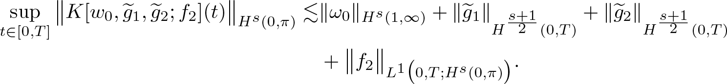 \begin{align*}
\sup\limits_{t\in[0,T]}\big\|K[w_0, \widetilde{g}_1,\widetilde{g}_2; f_2](t)\big\|_{H^s(0,\pi)}
\lesssim &
\|\omega_0\|_{H^s(1,\infty)}
+
\|\widetilde{g}_1\|_{H^{\frac{s+1}{2}}(0,T)}
+
\|\widetilde{g}_2\|_{H^{\frac{s+1}{2}}(0,T)}\\&
+
\big\|f_2\big\|_{L^1\big(0,T; H^s(0,\pi)\big)}.
\end{align*}
\begin{align*}
\sup\limits_{t\in[0,T]}\big\|K[w_0, \widetilde{g}_1,\widetilde{g}_2; f_2](t)\big\|_{H^s(0,\pi)}
\lesssim &
\|\omega_0\|_{H^s(1,\infty)}
+
\|\widetilde{g}_1\|_{H^{\frac{s+1}{2}}(0,T)}
+
\|\widetilde{g}_2\|_{H^{\frac{s+1}{2}}(0,T)}\\&
+
\big\|f_2\big\|_{L^1\big(0,T; H^s(0,\pi)\big)}.
\end{align*}4.2. Proof of well-posedness for ibvp in domain Ω2, i.e., theorem 1.3
Since the ibvp in Ω2 is reduced to the ibvp (2.1) for  $r \in ( \pi, 2\pi)$ with $u (\pi, t ) = g_1(t)$ and $u(2\pi, t)=g_2(t)$, it suffices to prove the well-posedness of ibvp (4.2) with forcing f 2 giving by
 \begin{equation}
f_2(r,t)
=
f_1(r+\pi,t)
=
-\lambda(r+\pi)^{-\frac{(n-1)(p-2)}2}|w|^{p-2}w+\frac{n^2-4n+3}{4}(r+\pi)^{-2}\cdot w.
\end{equation}
\begin{equation}
f_2(r,t)
=
f_1(r+\pi,t)
=
-\lambda(r+\pi)^{-\frac{(n-1)(p-2)}2}|w|^{p-2}w+\frac{n^2-4n+3}{4}(r+\pi)^{-2}\cdot w.
\end{equation} Furthermore, since both multipliers  $-(r+\pi)^{-\frac{(n-1)(p-2)}2}$ and $(r+\pi)^{-2}$ are smooth and bounded for $0 \lt r \lt \pi$, similar to the proof of theorem 1.2, we can bound them by using the $L^\infty$-norm. Therefore, the well-posedness proof is similar to the proof of theorem 4.10 and proposition 4.11 in [Reference Bona, Sun and Zhang7]. Hence, the details are omitted here.
5. ibvp in a ball centred at origin
In this section, we study the ibvp of (2.1) for  $r \in ( 0, 1)$. For the sake of convenience and simplicity, we only discuss the case with n = 2. The cases for $n\geq 3$ can be studied similarly.
5.1. Linear problem
The forced linear ibvp within the region Ω0 can be described by the following equations
 \begin{align}
&iu_t+\Delta u= f(x_1,x_2,t),
& &(x_1,x_2,t)\in \Omega_0,\,\,t\in(0,T),
\end{align}
\begin{align}
&iu_t+\Delta u= f(x_1,x_2,t),
& &(x_1,x_2,t)\in \Omega_0,\,\,t\in(0,T),
\end{align} \begin{align}
&u(x_1,x_2, 0 )
=
u_0(x_1,x_2),
& &(x_1,x_2)\in \Omega_0,
\end{align}
\begin{align}
&u(x_1,x_2, 0 )
=
u_0(x_1,x_2),
& &(x_1,x_2)\in \Omega_0,
\end{align} \begin{align}
&u(x_1,x_2,t) = g(t), & & x_1^2+x_2^2=1, \,\, t\in(0,T).
\end{align}
\begin{align}
&u(x_1,x_2,t) = g(t), & & x_1^2+x_2^2=1, \,\, t\in(0,T).
\end{align}We also decompose the ibvp (5.1) into the following two separate problems.
Problem 1. ibvp with homogeneous boundary condition
 \begin{align}
&iu_t+\Delta u= f(x_1,x_2,t),
& &(x_1,x_2,t)\in \Omega_0,\,\,t\in(0,T),
\end{align}
\begin{align}
&iu_t+\Delta u= f(x_1,x_2,t),
& &(x_1,x_2,t)\in \Omega_0,\,\,t\in(0,T),
\end{align} \begin{align}
&u(x_1,x_2, 0 )
=
u_0(x_1,x_2),
& &(x_1,x_2)\in \Omega_0,
\end{align}
\begin{align}
&u(x_1,x_2, 0 )
=
u_0(x_1,x_2),
& &(x_1,x_2)\in \Omega_0,
\end{align} \begin{align}
&u(x_1,x_2,t) = 0, & & x_1^2+x_2^2=1, \,\, t\in(0,T).
\end{align}
\begin{align}
&u(x_1,x_2,t) = 0, & & x_1^2+x_2^2=1, \,\, t\in(0,T).
\end{align}Problem 2. ibvp with non-homogeneous boundary condition
 \begin{align}
&iu_t+\Delta u= 0,
& &(x_1,x_2,t)\in \Omega_0,\,\,t\in(0,T),
\end{align}
\begin{align}
&iu_t+\Delta u= 0,
& &(x_1,x_2,t)\in \Omega_0,\,\,t\in(0,T),
\end{align} \begin{align}
&u(x_1,x_2, 0)
=
0,
& &(x_1,x_2)\in \Omega_0,
\end{align}
\begin{align}
&u(x_1,x_2, 0)
=
0,
& &(x_1,x_2)\in \Omega_0,
\end{align} \begin{align}
&u(x_1,x_2,t) = g(t), & & x_1^2+x_2^2=1, \,\, t\in(0,T).
\end{align}
\begin{align}
&u(x_1,x_2,t) = g(t), & & x_1^2+x_2^2=1, \,\, t\in(0,T).
\end{align}In the subsequent sections, we will investigate these two problems separately.
Estimate for Problem 1. In order to analyse this problem, we will employ the semigroup method. Following the methodology outlined in [Reference Cazenave11] (refer to section 2.1), we introduce the operator A acting on functions in  $L^2(\Omega_0)$, defined as follows:
 \begin{equation}
\begin{cases}
D(A)
=
\big\{
u\in H_0^1(\Omega_0),
\,\,
\Delta u\in L^2(\Omega_0)
\big\},
\\
A(u)
=
\Delta u
\quad
\text{for}
\,\,
u\in D(A).
\end{cases}
\end{equation}
\begin{equation}
\begin{cases}
D(A)
=
\big\{
u\in H_0^1(\Omega_0),
\,\,
\Delta u\in L^2(\Omega_0)
\big\},
\\
A(u)
=
\Delta u
\quad
\text{for}
\,\,
u\in D(A).
\end{cases}
\end{equation} It is worth noting that  $D(A) = H^2(\Omega_0)\cap H_0^1(\Omega_0)$. Additionally, we observe that A is a self-adjoint operator and $A\le 0$, as indicated by the following
 \begin{equation*} \lt Au,v \gt = \lt \Delta u, v \gt =
- \lt \nabla u, \nabla v \gt = \lt u,\Delta v \gt = \lt u, A^*v \gt \Longrightarrow
A=A^*,
\end{equation*}
\begin{equation*} \lt Au,v \gt = \lt \Delta u, v \gt =
- \lt \nabla u, \nabla v \gt = \lt u,\Delta v \gt = \lt u, A^*v \gt \Longrightarrow
A=A^*,
\end{equation*}and
 \begin{equation*} \lt Au,u \gt =
- \lt \nabla u, \nabla u \gt \le
0
\Longrightarrow
A\le 0.
\end{equation*}
\begin{equation*} \lt Au,u \gt =
- \lt \nabla u, \nabla u \gt \le
0
\Longrightarrow
A\le 0.
\end{equation*} Moreover, let  $(\mathcal{J}(t))_{t\in {\mathbb R}}$ represent the group of isometries generated by iA within any of the following spaces: D(A), $H_0^1(\Omega_0)$, $L^2(\Omega_0)$, $H^{-1}(\Omega_0)$, or $(D(A))^*$. By utilizing the property that iA is skew-adjoint, i.e.,
  $
(iA)^*
=
-iA,
$ we deduce the following relation
$
(iA)^*
=
-iA,
$ we deduce the following relation
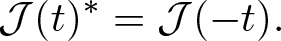 \begin{equation}
\mathcal{J}(t)^*
=
\mathcal{J}(-t).
\end{equation}
\begin{equation}
\mathcal{J}(t)^*
=
\mathcal{J}(-t).
\end{equation}Furthermore, the solution for the forced linear ibvp (5.2) is defined by
 \begin{equation}
u(x,t)
=
S_J[u_0; f]
\doteq
\mathcal{J}(t) u_0(x)
+
i
\int_0^t
\mathcal{J}(t-s)
f(x,s)
ds,
\quad
x\in \Omega_0,
\quad
t\in[0,T].
\end{equation}
\begin{equation}
u(x,t)
=
S_J[u_0; f]
\doteq
\mathcal{J}(t) u_0(x)
+
i
\int_0^t
\mathcal{J}(t-s)
f(x,s)
ds,
\quad
x\in \Omega_0,
\quad
t\in[0,T].
\end{equation}With these foundations in place, we can now proceed to establish the following results.
Proposition 5.1. If  $u_0\in L^2(\Omega_0)$ and $f\in L^1_t\big(0,T; L_x^2(\Omega_0)\big)$, then we have $S_J[u_0; f]\in C([0,T]; L_x^2(\Omega_0)) $ and it satisfies the following estimate
 \begin{equation}
\sup\limits_{t\in[0,T]}
\|S_J[u_0; f] (\cdot,t)\|_{L_x^2(\Omega_0)}
\lesssim
\|u_0\|_{L^2(\Omega_0)}
+
\|f(\cdot, t)\|_{L^1_t\big(0,T; L_x^2(\Omega_0)\big)}.
\end{equation}
\begin{equation}
\sup\limits_{t\in[0,T]}
\|S_J[u_0; f] (\cdot,t)\|_{L_x^2(\Omega_0)}
\lesssim
\|u_0\|_{L^2(\Omega_0)}
+
\|f(\cdot, t)\|_{L^1_t\big(0,T; L_x^2(\Omega_0)\big)}.
\end{equation} In addition, if  $u_0\in H_0^2(\Omega_0)$ and $f\in L_t^1\big(0,T; H_0^2(\Omega_0)\big)$, then we have $S_J[u_0; f]\in C([0,T]; H_0^2(\Omega_0)) $ and it satisfies the following estimate
 \begin{equation}
\sup\limits_{t\in[0,T]}
\|S_J[u_0; f] (\cdot,t)\|_{H^2(\Omega_0)}
\lesssim
\|u_0\|_{H^2(\Omega_0)}
+
\|f(\cdot, t)\|_{L_t^1\big(0,T; H^2(\Omega_0)\big)}.
\end{equation}
\begin{equation}
\sup\limits_{t\in[0,T]}
\|S_J[u_0; f] (\cdot,t)\|_{H^2(\Omega_0)}
\lesssim
\|u_0\|_{H^2(\Omega_0)}
+
\|f(\cdot, t)\|_{L_t^1\big(0,T; H^2(\Omega_0)\big)}.
\end{equation} Finally, for  $1 \lt s \lt 2$, if $u_0\in H_0^s(\Omega_0)$ and $f\in L_t^1\big(0,T; H_0^s(\Omega_0)\big)$, then we have $S_J[u_0; f]\in C([0,T]; H_0^s(\Omega_0)) $ and it satisfies the following estimate
 \begin{equation}
\sup\limits_{t\in[0,T]}
\|S_J[u_0; f] (\cdot,t)\|_{H^s(\Omega_0)}
\lesssim
\|u_0\|_{H^s(\Omega_0)}
+
\|f(\cdot, t)\|_{L_t^1\big(0,T; H^s(\Omega_0)\big)}.
\end{equation}
\begin{equation}
\sup\limits_{t\in[0,T]}
\|S_J[u_0; f] (\cdot,t)\|_{H^s(\Omega_0)}
\lesssim
\|u_0\|_{H^s(\Omega_0)}
+
\|f(\cdot, t)\|_{L_t^1\big(0,T; H^s(\Omega_0)\big)}.
\end{equation}Proof 5.1. Proof of proposition 5.1
The proof of estimate (5.9) can be deduced through interpolation and the estimates (5.7) and (5.8). Additionally, the proof of estimate (5.8) closely parallels the proof of estimate (5.7). Therefore, in this exposition, we shall exclusively present the proof for estimate (5.7). Using the relation (5.5), we obtain
 \begin{align*} \lt \mathcal{J}(t) u_0(x), \mathcal{J}(t) u_0(x) \gt _{L^2(\Omega_0)}
=& \lt u_0(x), \mathcal{J}(t)^*\mathcal{J}(t) u_0(x) \gt _{L^2(\Omega_0)}
\\
=& \lt u_0(x), \mathcal{J}(-t)\mathcal{J}(t) u_0(x) \gt _{L^2(\Omega_0)}\\
=& \lt u_0(x), u_0(x) \gt _{L^2(\Omega_0)}.
\end{align*}
\begin{align*} \lt \mathcal{J}(t) u_0(x), \mathcal{J}(t) u_0(x) \gt _{L^2(\Omega_0)}
=& \lt u_0(x), \mathcal{J}(t)^*\mathcal{J}(t) u_0(x) \gt _{L^2(\Omega_0)}
\\
=& \lt u_0(x), \mathcal{J}(-t)\mathcal{J}(t) u_0(x) \gt _{L^2(\Omega_0)}\\
=& \lt u_0(x), u_0(x) \gt _{L^2(\Omega_0)}.
\end{align*}This gives us that
 \begin{equation}
\sup\limits_{t\in[0,T]}
\|\mathcal{J}(t) u_0(\cdot )\|_{L^2(\Omega_0)}
=
\|u_0\|_{L^2(\Omega_0)}.
\end{equation}
\begin{equation}
\sup\limits_{t\in[0,T]}
\|\mathcal{J}(t) u_0(\cdot )\|_{L^2(\Omega_0)}
=
\|u_0\|_{L^2(\Omega_0)}.
\end{equation}Using the identity (5.10), we derive
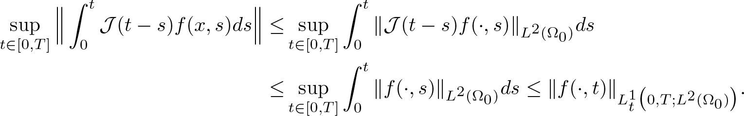 \begin{align}
\sup\limits_{t\in[0,T]}
\Big\|
\int_0^t
\mathcal{J}(t-s)
f(x,s)
ds
\Big\|
\le&
\sup\limits_{t\in[0,T]}
\int_0^t
\|
\mathcal{J}(t-s)
f(\cdot,s)
\|_{L^2(\Omega_0)}
ds
\nonumber
\\
\le&
\sup\limits_{t\in[0,T]}
\int_0^t
\|f(\cdot,s)\|_{L^2(\Omega_0)}
ds
\le
\|f(\cdot, t)\|_{L_t^1\big(0,T; L^2(\Omega_0)\big)}.
\end{align}
\begin{align}
\sup\limits_{t\in[0,T]}
\Big\|
\int_0^t
\mathcal{J}(t-s)
f(x,s)
ds
\Big\|
\le&
\sup\limits_{t\in[0,T]}
\int_0^t
\|
\mathcal{J}(t-s)
f(\cdot,s)
\|_{L^2(\Omega_0)}
ds
\nonumber
\\
\le&
\sup\limits_{t\in[0,T]}
\int_0^t
\|f(\cdot,s)\|_{L^2(\Omega_0)}
ds
\le
\|f(\cdot, t)\|_{L_t^1\big(0,T; L^2(\Omega_0)\big)}.
\end{align}Combining estimates (5.10) with (5.11), we establish the inequality (5.7). This concludes the proof of proposition 5.1
Estimate for Problem 2. We initiate our analysis by finding the solution to the ibvp (5.3). Utilizing the expression  $\Delta u = u''(r) + \frac{1}{r}u'(r)$, we reformulate this ibvp as follows
 \begin{align}
&iu_t
+
u_{rr} + \frac{1}{r} u_r =0,
& &
0 \lt r \lt 1,
\,\,
t\in(0,T),
\end{align}
\begin{align}
&iu_t
+
u_{rr} + \frac{1}{r} u_r =0,
& &
0 \lt r \lt 1,
\,\,
t\in(0,T),
\end{align} \begin{align}
&u(r,0)
=
0
,
& &
0 \lt r \lt 1,
\end{align}
\begin{align}
&u(r,0)
=
0
,
& &
0 \lt r \lt 1,
\end{align} \begin{align}
&u(1,t)
=
h(t),
&
&
t\in{\mathbb R}.
\end{align}
\begin{align}
&u(1,t)
=
h(t),
&
&
t\in{\mathbb R}.
\end{align} Here, h(t) extends the boundary data g(t) from the interval  $(0, T)$ to the entire real line ${\mathbb R}$. By making use of lemma 3.3, we assume that h is compactly supported in the interval $(0, 2)$. Additionally, at r = 0, the equation in (5.12) implies the following boundary condition
 \begin{equation}
u_r(0,t)
=
0.
\end{equation}
\begin{equation}
u_r(0,t)
=
0.
\end{equation}We will solve the reduced pure ibvp (5.12) and commence with solving the following ibvp
 \begin{align}
&iU_t
+
U_{rr} + \frac{1}{r} U_r =0,
& &
0 \lt r \lt 1,
\,\,
t\in(0,T),
\end{align}
\begin{align}
&iU_t
+
U_{rr} + \frac{1}{r} U_r =0,
& &
0 \lt r \lt 1,
\,\,
t\in(0,T),
\end{align} \begin{align}
&U(r,0)
=
U_0(r)
,
& &
0 \lt r \lt 1,
\end{align}
\begin{align}
&U(r,0)
=
U_0(r)
,
& &
0 \lt r \lt 1,
\end{align} \begin{align}
&
U_r(0,t)=U(1,t)
=
0,
& &
t\in (0,T).
\end{align}
\begin{align}
&
U_r(0,t)=U(1,t)
=
0,
& &
t\in (0,T).
\end{align}By employing the standard method of separation of variables, we can find the general solution for (5.14) as
 \begin{equation}
U(r,t)
=
S_{ball}(t)U_0(r)
\doteq
\sum\limits_{n=0}^\infty
\beta_n
J_0(\lambda_n r)
e^{-i\lambda_n^2t}\, ,
\end{equation}
\begin{equation}
U(r,t)
=
S_{ball}(t)U_0(r)
\doteq
\sum\limits_{n=0}^\infty
\beta_n
J_0(\lambda_n r)
e^{-i\lambda_n^2t}\, ,
\end{equation} where  $J_0(z)$ represents the Bessel function of order 0, and $\lambda_n, n=0,1,2,\ldots,$ are the positive zeros of the Bessel function J 0, meaning $J_0(\lambda_n ) = 0$. The coefficients $\beta_n, n = 0, 1, \ldots,$ are determined by the initial condition $U_0(r)$ and can be calculated as follows
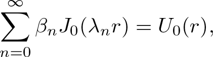 \begin{equation*}
\sum\limits_{n=0}^\infty
\beta_n
J_0(\lambda_n r)
=
U_0(r),
\end{equation*}
\begin{equation*}
\sum\limits_{n=0}^\infty
\beta_n
J_0(\lambda_n r)
=
U_0(r),
\end{equation*}which gives us that
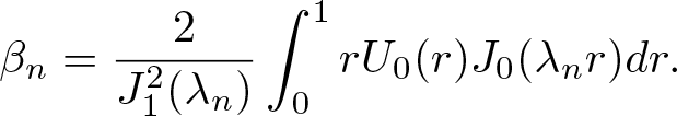 \begin{equation}
\beta_n
=
\frac{2}{J_{1}^{2}(\lambda_{n})}
\int_0^1
r
U_0(r) J_0(\lambda_n r) dr.
\end{equation}
\begin{equation}
\beta_n
=
\frac{2}{J_{1}^{2}(\lambda_{n})}
\int_0^1
r
U_0(r) J_0(\lambda_n r) dr.
\end{equation}Remark 5.2. The Fourier–Bessel series for a function f(x) on the interval  $(0,1)$ with respect to the Bessel function J 0 can be expressed as:
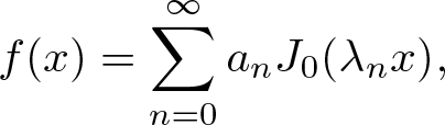 \begin{equation*}
f(x) = \sum_{n=0}^{\infty} a_n J_0(\lambda_n x),
\end{equation*}
\begin{equation*}
f(x) = \sum_{n=0}^{\infty} a_n J_0(\lambda_n x),
\end{equation*}where the coefficients an are given by
 \begin{equation}
a_n
=
\frac{2}{J_{1}^{2}(\lambda_{n})}
\int_0^1
x
f(x) J_0(\lambda_n x) dx,
\end{equation}
\begin{equation}
a_n
=
\frac{2}{J_{1}^{2}(\lambda_{n})}
\int_0^1
x
f(x) J_0(\lambda_n x) dx,
\end{equation} and  $\lambda_n, n=0,1,2,\ldots,$ are the positive zeros of the Bessel function J 0, i.e., $J_0(\lambda_n) = 0$.
Remark 5.3. The Bessel functions  $J_0(\lambda_nx), n= 0, 1, 2, \ldots, $ are orthogonal over the interval $(0,1)$ with respect to the weight function x, meaning:
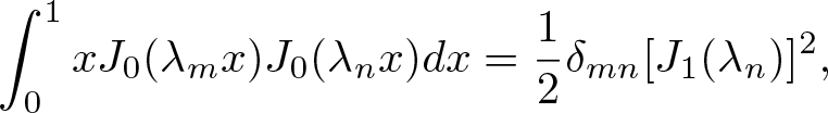 \begin{equation}
\int_{0}^{1}
x
J_0(\lambda_m x) J_0(\lambda_n x) dx
=
\frac{1}{2} \delta_{mn}
[J_1(\lambda_n)]^2,
\end{equation}
\begin{equation}
\int_{0}^{1}
x
J_0(\lambda_m x) J_0(\lambda_n x) dx
=
\frac{1}{2} \delta_{mn}
[J_1(\lambda_n)]^2,
\end{equation}where δmn is the Kronecker delta, defined as:
 \begin{equation*}
\delta_{mn}
=
\begin{cases}
1 & \text{if } m=n,
\\
0 & \text{otherwise}.
\end{cases}
\end{equation*}
\begin{equation*}
\delta_{mn}
=
\begin{cases}
1 & \text{if } m=n,
\\
0 & \text{otherwise}.
\end{cases}
\end{equation*} This allows us to express the coefficient an in terms of inner products of f(x) with the Bessel function  $J_0(\lambda_nx)$.
Solving forced ibvp. Now, let us address the following forced problem
 \begin{align}
&iV_t
+
V_{rr} + \frac{1}{r} V_r =F(r,t),
& &
0 \lt r \lt 1,
\,\,
t\in(0,T),
\end{align}
\begin{align}
&iV_t
+
V_{rr} + \frac{1}{r} V_r =F(r,t),
& &
0 \lt r \lt 1,
\,\,
t\in(0,T),
\end{align} \begin{align}
&V(r,0)
=
0
,
& &
0 \lt r \lt 1,
\end{align}
\begin{align}
&V(r,0)
=
0
,
& &
0 \lt r \lt 1,
\end{align} \begin{align}
&
V_r(0,t)=V(1,t)
=
0,
& &
t\in (0,T).
\end{align}
\begin{align}
&
V_r(0,t)=V(1,t)
=
0,
& &
t\in (0,T).
\end{align}Utilizing Duhamel’s principle, the solution to the forced ibvp (5.19) is given by
 \begin{equation}
V(r,t)
=
-i
\int_0^t
S_{ball}(t-t')F(r,t')
dt'
\doteq
-i
\sum\limits_{n=0}^\infty
J_0(\lambda_n r)
\int_0^t
e^{-i\lambda_n^2(t-t')}
B_n(t')
dt',
\end{equation}
\begin{equation}
V(r,t)
=
-i
\int_0^t
S_{ball}(t-t')F(r,t')
dt'
\doteq
-i
\sum\limits_{n=0}^\infty
J_0(\lambda_n r)
\int_0^t
e^{-i\lambda_n^2(t-t')}
B_n(t')
dt',
\end{equation}where
 \begin{equation}
B_n(t')
=
\frac{2}{J_{1}^{2}(\lambda_{n})} \int_0^1
r
F(r,t') J_0(\lambda_n r) dr.
\end{equation}
\begin{equation}
B_n(t')
=
\frac{2}{J_{1}^{2}(\lambda_{n})} \int_0^1
r
F(r,t') J_0(\lambda_n r) dr.
\end{equation} Solving ibvp (5.12). Defining  $v(r,t) = u(r,t) - h(t)$, we obtain the ibvp for v as follows
 \begin{align}
&iv_t
+
v_{rr} + \frac{1}{r} v_r =F_h(r,t),
& &
0 \lt r \lt 1,
\,\,
t\in(0,T),
\end{align}
\begin{align}
&iv_t
+
v_{rr} + \frac{1}{r} v_r =F_h(r,t),
& &
0 \lt r \lt 1,
\,\,
t\in(0,T),
\end{align} \begin{align}
&v(r,0)
=
0
,
& &
0 \lt r \lt 1,
\end{align}
\begin{align}
&v(r,0)
=
0
,
& &
0 \lt r \lt 1,
\end{align} \begin{align}
&
v_r(0,t)=v(1,t)
=
0,
& &
t\in (0,T),
\end{align}
\begin{align}
&
v_r(0,t)=v(1,t)
=
0,
& &
t\in (0,T),
\end{align} where  $F_h = -ih'(t)$. Employing the solution formula (5.20) with $F = F_h$, we have
 \begin{align}
v
=
-
\sum\limits_{n=0}^\infty
J_0(\lambda_n r)
b_{n}
\int_0^t
h'(t')
e^{-i\lambda_n^2(t-t')}
dt',
\end{align}
\begin{align}
v
=
-
\sum\limits_{n=0}^\infty
J_0(\lambda_n r)
b_{n}
\int_0^t
h'(t')
e^{-i\lambda_n^2(t-t')}
dt',
\end{align}where bn represents the Fourier–Bessel coefficient of 1, and can be computed as
 \begin{align}
b_{n}
=
\frac{2}{J_{1}^{2}(\lambda_{n})}
\int_0^1
r
\cdot J_0(\lambda_n r) dr
=
\frac{2}{J_{1}^{2}(\lambda_{n})}
\cdot
\frac{J_{1}(\lambda_{n})}{\lambda_{n}}
=
\frac{2}{J_{1}(\lambda_{n})\lambda_n}.
\end{align}
\begin{align}
b_{n}
=
\frac{2}{J_{1}^{2}(\lambda_{n})}
\int_0^1
r
\cdot J_0(\lambda_n r) dr
=
\frac{2}{J_{1}^{2}(\lambda_{n})}
\cdot
\frac{J_{1}(\lambda_{n})}{\lambda_{n}}
=
\frac{2}{J_{1}(\lambda_{n})\lambda_n}.
\end{align} Further, by performing integration by parts and utilizing the initial condition  $h(0) = 0$, we obtain
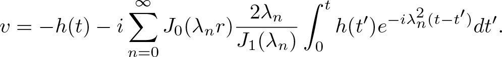 \begin{align}
v
=
-
h(t)
-
i
\sum\limits_{n=0}^\infty
J_0(\lambda_n r)
\frac{2 \lambda_n}{J_{1}(\lambda_{n})}
\int_0^t
h(t')
e^{-i\lambda_n^2(t-t')}
dt'.
\end{align}
\begin{align}
v
=
-
h(t)
-
i
\sum\limits_{n=0}^\infty
J_0(\lambda_n r)
\frac{2 \lambda_n}{J_{1}(\lambda_{n})}
\int_0^t
h(t')
e^{-i\lambda_n^2(t-t')}
dt'.
\end{align} Therefore, the solution to the ibvp (5.12), denoted as  $u = v + h$, is expressed as
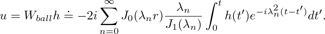 \begin{align}
u
=
W_{ball}h
\doteq
-
2
i
\sum\limits_{n=0}^\infty
J_0(\lambda_n r)
\frac{\lambda_n}{J_{1}(\lambda_{n})}
\int_0^t
h(t')
e^{-i\lambda_n^2(t-t')}
dt'.
\end{align}
\begin{align}
u
=
W_{ball}h
\doteq
-
2
i
\sum\limits_{n=0}^\infty
J_0(\lambda_n r)
\frac{\lambda_n}{J_{1}(\lambda_{n})}
\int_0^t
h(t')
e^{-i\lambda_n^2(t-t')}
dt'.
\end{align} In addition, if we switch back to the variables  $(x_1, x_2)$, then we have
 \begin{align}
u(x_1,x_2,t)
=
W_{ball}h
\doteq
-
2
i
\sum\limits_{n=0}^\infty
J_0\Big(\lambda_n \sqrt{x_1^2+x_2^2}\Big)
\frac{\lambda_n}{J_{1}(\lambda_{n})}
\int_0^t
h(t')
e^{-i\lambda_n^2(t-t')}
dt'.
\end{align}
\begin{align}
u(x_1,x_2,t)
=
W_{ball}h
\doteq
-
2
i
\sum\limits_{n=0}^\infty
J_0\Big(\lambda_n \sqrt{x_1^2+x_2^2}\Big)
\frac{\lambda_n}{J_{1}(\lambda_{n})}
\int_0^t
h(t')
e^{-i\lambda_n^2(t-t')}
dt'.
\end{align}Next, we will prove the following result.
Proposition 5.4. Let  $h\in H^{1/2}_{00}(0,T)$. Then, the solution defined by (5.26) satisfies the following estimate
 \begin{align}
\sup\limits_{t\in[0,T]}\Big\|
r^{1/2}
\cdot
W_{ball}
h
\Big\|_{L^2(0,1)}
\lesssim
\|h\|_{H^{1/2}(0,T)}.
\end{align}
\begin{align}
\sup\limits_{t\in[0,T]}\Big\|
r^{1/2}
\cdot
W_{ball}
h
\Big\|_{L^2(0,1)}
\lesssim
\|h\|_{H^{1/2}(0,T)}.
\end{align} Furthermore, if  $h \in H^{(s+1)/2}_{0}(0, T)$ for $0\le s \le 2$ (for $s=0,2$, $ h\in H_{00}^{\frac{s+1}{2}}(0,T)$), then the solution defined by (5.27) satisfies the following estimates
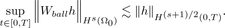 \begin{align}
\sup\limits_{t\in[0,T]}\Big\|
W_{ball}
h
\Big\|_{H^s (\Omega_0) }
\lesssim
\|h\|_{H^{(s+1)/2}(0,T)}.
\end{align}
\begin{align}
\sup\limits_{t\in[0,T]}\Big\|
W_{ball}
h
\Big\|_{H^s (\Omega_0) }
\lesssim
\|h\|_{H^{(s+1)/2}(0,T)}.
\end{align}To show the above result, we need Parseval’s identity for Fourier–Bessel series, which is stated as follows.
Lemma 5.5. Let  $x^{1/2}f(x)\in L^2(0,1)$. If the Fourier–Bessel series of f(x) is given by
 \begin{equation*}
f(x)
=
\sum\limits_{n=0}^\infty
c_n J_0(\lambda_n r),
\end{equation*}
\begin{equation*}
f(x)
=
\sum\limits_{n=0}^\infty
c_n J_0(\lambda_n r),
\end{equation*} where  $c_n=\frac{2}{J_{1}^{2}(\lambda_{n})} \int_0^1
xf(x) J_0(\lambda_n x) dx\, ,$ then we have
$c_n=\frac{2}{J_{1}^{2}(\lambda_{n})} \int_0^1
xf(x) J_0(\lambda_n x) dx\, ,$ then we have
 \begin{equation}
\int_0^1
x
|f(x)|^2
dx
=
\frac12
\sum\limits_{n=0}^\infty
|c_n|^2
[J_1(\lambda_n)]^2.
\end{equation}
\begin{equation}
\int_0^1
x
|f(x)|^2
dx
=
\frac12
\sum\limits_{n=0}^\infty
|c_n|^2
[J_1(\lambda_n)]^2.
\end{equation}Proof 5.1. Proof of lemma 5.5
By straightforward computation, we get
 \begin{align*}
\int_0^1
x
|f(x)|^2
dx
=
\int_0^1
x
f(x)
\overline{f(x)}
dx
=
\sum\limits_{n=0}^\infty
\sum\limits_{m=0}^\infty
c_n c_m
\int_0^1
x
J_0(\lambda_nx)
J_0(\lambda_mx)
dx.
\end{align*}
\begin{align*}
\int_0^1
x
|f(x)|^2
dx
=
\int_0^1
x
f(x)
\overline{f(x)}
dx
=
\sum\limits_{n=0}^\infty
\sum\limits_{m=0}^\infty
c_n c_m
\int_0^1
x
J_0(\lambda_nx)
J_0(\lambda_mx)
dx.
\end{align*}Now, applying the orthogonal identity (5.18), i.e.,
 \begin{equation}
\int_{0}^{1}
x
J_0(\lambda_m x) J_0(\lambda_n x) dx
=
\frac{1}{2} \delta_{mn}
[J_1(\lambda_n)]^2,
\end{equation}
\begin{equation}
\int_{0}^{1}
x
J_0(\lambda_m x) J_0(\lambda_n x) dx
=
\frac{1}{2} \delta_{mn}
[J_1(\lambda_n)]^2,
\end{equation}we obtain the desired identity (5.30). This completes the proof of lemma 5.5.
Proof 5.1. Proof of proposition 5.4
We will begin by providing the proof of estimate (5.28), which is similar to the proof of estimate (4.43). We start by expressing  $h(t')$ as follows
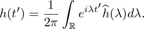 \begin{equation*}
h(t')=\frac1{2\pi}\int_{{\mathbb R}}e^{i\lambda t'}\widehat{h}(\lambda)d\lambda.
\end{equation*}
\begin{equation*}
h(t')=\frac1{2\pi}\int_{{\mathbb R}}e^{i\lambda t'}\widehat{h}(\lambda)d\lambda.
\end{equation*}Using this expression and formula (5.26), we can write
 \begin{equation}
\psi
\cdot
W_{ball}
h
=
\frac{-i\psi(t)}{\pi}
\sum\limits_{n=0}^\infty
J_0(\lambda_n r)
\frac{\lambda_n}{J_{1}(\lambda_{n})}
\int_0^t
e^{-i \lambda_n^2 (t-t') }
\int_{{\mathbb R}}e^{i\lambda t'}\widehat{h}(\lambda)d\lambda
dt'.
\end{equation}
\begin{equation}
\psi
\cdot
W_{ball}
h
=
\frac{-i\psi(t)}{\pi}
\sum\limits_{n=0}^\infty
J_0(\lambda_n r)
\frac{\lambda_n}{J_{1}(\lambda_{n})}
\int_0^t
e^{-i \lambda_n^2 (t-t') }
\int_{{\mathbb R}}e^{i\lambda t'}\widehat{h}(\lambda)d\lambda
dt'.
\end{equation}Now, let us perform the integration with respect to t ʹ using the computation
 \begin{align*}
\int_0^t e^{i(\lambda+\lambda_n^2)t'}dt'
=
-i\frac{e^{i(\lambda+\lambda_n^2)t}-1}{\lambda+\lambda_n^2}.
\end{align*}
\begin{align*}
\int_0^t e^{i(\lambda+\lambda_n^2)t'}dt'
=
-i\frac{e^{i(\lambda+\lambda_n^2)t}-1}{\lambda+\lambda_n^2}.
\end{align*} With this, the expression for  $\psi(t)W_{\text{ball}}h$ becomes
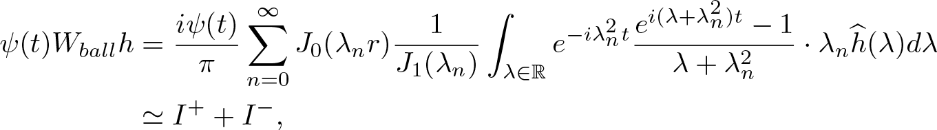 \begin{align}
\psi(t)
W_{ball}
h &
=
\frac{i\psi(t)}{\pi}\sum\limits_{n=0}^\infty
J_0(\lambda_n r)
\frac{1}{J_1(\lambda_n)}
\int_{\lambda\in{\mathbb R}}
e^{-i\lambda_n^2t}\frac{e^{i(\lambda+\lambda_n^2)t}-1}{\lambda+\lambda_n^2}
\cdot
\lambda_n
\widehat{h}(\lambda)d\lambda\\&
\simeq
I^++I^-,
\end{align}
\begin{align}
\psi(t)
W_{ball}
h &
=
\frac{i\psi(t)}{\pi}\sum\limits_{n=0}^\infty
J_0(\lambda_n r)
\frac{1}{J_1(\lambda_n)}
\int_{\lambda\in{\mathbb R}}
e^{-i\lambda_n^2t}\frac{e^{i(\lambda+\lambda_n^2)t}-1}{\lambda+\lambda_n^2}
\cdot
\lambda_n
\widehat{h}(\lambda)d\lambda\\&
\simeq
I^++I^-,
\end{align} where  $I^{+}$ is the integral over $(0,\infty)$ and $I^{-}$ is the integral over $(-\infty,0)$. More precisely, we have
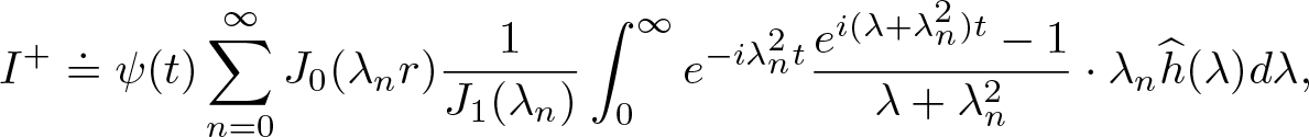 \begin{align}
I^+
\doteq
\psi(t)\sum\limits_{n=0}^\infty
J_0(\lambda_n r)
\frac{1}{J_1(\lambda_n)}
\int_{0}^\infty
e^{-i\lambda_n^2t}\frac{e^{i(\lambda+\lambda_n^2)t}-1}{\lambda+\lambda_n^2}
\cdot
\lambda_n
\widehat{h}(\lambda)d\lambda,
\end{align}
\begin{align}
I^+
\doteq
\psi(t)\sum\limits_{n=0}^\infty
J_0(\lambda_n r)
\frac{1}{J_1(\lambda_n)}
\int_{0}^\infty
e^{-i\lambda_n^2t}\frac{e^{i(\lambda+\lambda_n^2)t}-1}{\lambda+\lambda_n^2}
\cdot
\lambda_n
\widehat{h}(\lambda)d\lambda,
\end{align}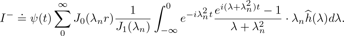 \begin{align}
I^-
\doteq
\psi(t)\sum\limits_{0}^\infty
J_0(\lambda_n r)
\frac{1}{J_1(\lambda_n)}
\int_{-\infty}^0
e^{-i\lambda_n^2t}\frac{e^{i(\lambda+\lambda_n^2)t}-1}{\lambda+\lambda_n^2}
\cdot
\lambda_n
\widehat{h}(\lambda)d\lambda.
\end{align}
\begin{align}
I^-
\doteq
\psi(t)\sum\limits_{0}^\infty
J_0(\lambda_n r)
\frac{1}{J_1(\lambda_n)}
\int_{-\infty}^0
e^{-i\lambda_n^2t}\frac{e^{i(\lambda+\lambda_n^2)t}-1}{\lambda+\lambda_n^2}
\cdot
\lambda_n
\widehat{h}(\lambda)d\lambda.
\end{align} Estimate of weighted L 2-norm for  $I^+$. Let
 \begin{equation*}
f(r,t)
=
r^{1/2}
\cdot
\sum\limits_{n=0}^\infty
J_0(\lambda_n r)
\frac{1}{J_1(\lambda_n)}
\int_{0}^\infty
e^{-i\lambda_n^2t}\frac{e^{i(\lambda+\lambda_n^2)t}-1}{\lambda+\lambda_n^2}
\cdot
\lambda_n
\widehat{h}(\lambda)d\lambda.
\end{equation*}
\begin{equation*}
f(r,t)
=
r^{1/2}
\cdot
\sum\limits_{n=0}^\infty
J_0(\lambda_n r)
\frac{1}{J_1(\lambda_n)}
\int_{0}^\infty
e^{-i\lambda_n^2t}\frac{e^{i(\lambda+\lambda_n^2)t}-1}{\lambda+\lambda_n^2}
\cdot
\lambda_n
\widehat{h}(\lambda)d\lambda.
\end{equation*} First, we prove L 2 estimate (5.28) for  $I_1^{+}$. Since ψ is compactly supported in $(0,1)$, we have $\sup\limits_{t\in[0,T]}\|r^{1/2}\cdot I_1^{+}\|_{L^2(0,1)}\le \sup\limits_{t\in[0,1]}\|f\|_{L^2(0,1)}$. Using Parseval’s identity for Fourier–Bessel series (identity (5.30)), we get
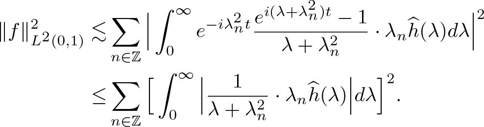 \begin{align}
\|f\|_{L^2(0,1)}^2
\lesssim&
\sum\limits_{n\in{\mathbb Z}}
\Big|
\int_{0}^\infty
e^{-i\lambda_n^2t}\frac{e^{i(\lambda+\lambda_n^2)t}-1}{\lambda+\lambda_n^2}
\cdot
\lambda_n
\widehat{h}(\lambda)d\lambda
\Big|^2\\
\le &
\sum\limits_{n\in{\mathbb Z}}
\Big[
\int_{0}^\infty
\Big|
\frac{1}{\lambda+\lambda_n^2}
\cdot
\lambda_n
\widehat{h}(\lambda)
\Big|
d\lambda
\Big]^2.
\end{align}
\begin{align}
\|f\|_{L^2(0,1)}^2
\lesssim&
\sum\limits_{n\in{\mathbb Z}}
\Big|
\int_{0}^\infty
e^{-i\lambda_n^2t}\frac{e^{i(\lambda+\lambda_n^2)t}-1}{\lambda+\lambda_n^2}
\cdot
\lambda_n
\widehat{h}(\lambda)d\lambda
\Big|^2\\
\le &
\sum\limits_{n\in{\mathbb Z}}
\Big[
\int_{0}^\infty
\Big|
\frac{1}{\lambda+\lambda_n^2}
\cdot
\lambda_n
\widehat{h}(\lambda)
\Big|
d\lambda
\Big]^2.
\end{align} Now, applying Cauchy–Schwarz inequality in  $d\lambda$, for ɛ > 0 (small), we obtain
 \begin{align*}
\Big[
\int_{0}^\infty
\Big|
\frac{1}{\lambda+\lambda_n^2}
\cdot
\lambda_n
\widehat{h}(\lambda)
\Big|
d\lambda
\Big]^2
\le&
\int_{0}^{\infty}
\frac{\lambda_n^2(1+\lambda)^{2\varepsilon}}{(\lambda+\lambda_n^2)^2}
(1+\lambda)|\widehat{h}(\lambda)|^2
d\lambda
\cdot
\int_{0}^{\infty}
\frac{1}{(1+\lambda)^{1+2\varepsilon}}
d\lambda
\\
\lesssim&
\int_{0}^{\infty}
\frac{\lambda_n^2(1+\lambda)^{2\varepsilon}}{(\lambda+\lambda_n^2)^2}
(1+\lambda)|\widehat{h}(\lambda)|^2
d\lambda.
\end{align*}
\begin{align*}
\Big[
\int_{0}^\infty
\Big|
\frac{1}{\lambda+\lambda_n^2}
\cdot
\lambda_n
\widehat{h}(\lambda)
\Big|
d\lambda
\Big]^2
\le&
\int_{0}^{\infty}
\frac{\lambda_n^2(1+\lambda)^{2\varepsilon}}{(\lambda+\lambda_n^2)^2}
(1+\lambda)|\widehat{h}(\lambda)|^2
d\lambda
\cdot
\int_{0}^{\infty}
\frac{1}{(1+\lambda)^{1+2\varepsilon}}
d\lambda
\\
\lesssim&
\int_{0}^{\infty}
\frac{\lambda_n^2(1+\lambda)^{2\varepsilon}}{(\lambda+\lambda_n^2)^2}
(1+\lambda)|\widehat{h}(\lambda)|^2
d\lambda.
\end{align*}Thus, combining above estimates, it is deduced that
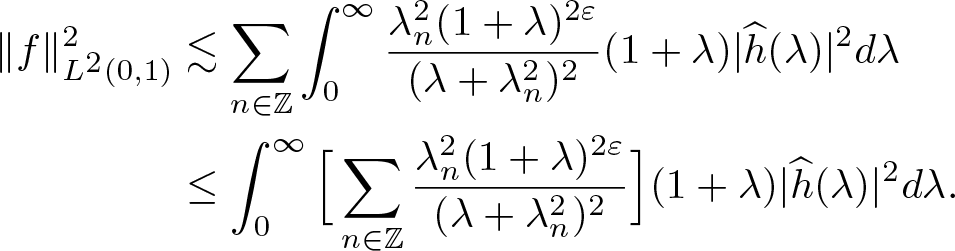 \begin{align*}
\|f\|_{L^2(0,1)}^2&
\lesssim
\sum\limits_{n\in{\mathbb Z}}
\int_{0}^{\infty}
\frac{\lambda_n^2(1+\lambda)^{2\varepsilon}}{(\lambda+\lambda_n^2)^2}
(1+\lambda)|\widehat{h}(\lambda)|^2
d\lambda \\&
\le
\int_{0}^{\infty}
\Big[
\sum\limits_{n\in{\mathbb Z}}
\frac{\lambda_n^2(1+\lambda)^{2\varepsilon}}{(\lambda+\lambda_n^2)^2}
\Big]
(1+\lambda)|\widehat{h}(\lambda)|^2
d\lambda.
\end{align*}
\begin{align*}
\|f\|_{L^2(0,1)}^2&
\lesssim
\sum\limits_{n\in{\mathbb Z}}
\int_{0}^{\infty}
\frac{\lambda_n^2(1+\lambda)^{2\varepsilon}}{(\lambda+\lambda_n^2)^2}
(1+\lambda)|\widehat{h}(\lambda)|^2
d\lambda \\&
\le
\int_{0}^{\infty}
\Big[
\sum\limits_{n\in{\mathbb Z}}
\frac{\lambda_n^2(1+\lambda)^{2\varepsilon}}{(\lambda+\lambda_n^2)^2}
\Big]
(1+\lambda)|\widehat{h}(\lambda)|^2
d\lambda.
\end{align*} Furthermore, using  $\lambda+\lambda_n^2\ge \max\{\lambda, \lambda_n^2\}$ and $\lambda_n\approx (n-\frac14)\pi\simeq n$, for all $\lambda\ge 0$ and $2-2\varepsilon \gt \frac32$ or $\varepsilon \lt \frac14$, we get
 \begin{align*}
\sum\limits_{n\in{\mathbb Z}}
\frac{\lambda_n^2(1+\lambda)^{2\varepsilon}}{(\lambda+\lambda_n^2)^2}
\le
\sum\limits_{n\in{\mathbb Z}}
\frac{\lambda_n^2}{(\lambda+\lambda_n^2)^{2-2\varepsilon}}
\cdot
\frac{(1+\lambda)^{2\varepsilon}}{(\lambda+\lambda_n^2)^{2\varepsilon}}
\lesssim
\sum\limits_{n\in{\mathbb Z}}
\frac{n^2}{(\lambda+n^2)^{\frac32+}}
\lesssim
\sum\limits_{n=1}^{\infty}
\frac{1}{n^{1+}}
\lesssim 1.
\end{align*}
\begin{align*}
\sum\limits_{n\in{\mathbb Z}}
\frac{\lambda_n^2(1+\lambda)^{2\varepsilon}}{(\lambda+\lambda_n^2)^2}
\le
\sum\limits_{n\in{\mathbb Z}}
\frac{\lambda_n^2}{(\lambda+\lambda_n^2)^{2-2\varepsilon}}
\cdot
\frac{(1+\lambda)^{2\varepsilon}}{(\lambda+\lambda_n^2)^{2\varepsilon}}
\lesssim
\sum\limits_{n\in{\mathbb Z}}
\frac{n^2}{(\lambda+n^2)^{\frac32+}}
\lesssim
\sum\limits_{n=1}^{\infty}
\frac{1}{n^{1+}}
\lesssim 1.
\end{align*} Therefore, the desired estimate (5.28) for  $I^{+}$ is obtained.
Estimate of weighted L 2-norm for  $I^-$. Adding and subtracting $\psi(\lambda+\lambda_n^2)$ inside the integral (localizing near the singularity $\lambda=-\lambda_n^2$) gives the following decomposition of $I^-$
$I^-$
 \begin{align}
I^-
=&
\psi(t)\sum\limits_{0}^\infty
J_0(\lambda_n r)
\frac{1}{J_1(\lambda_n)}
\int_{-\infty}^{0}
\big[
e^{-i\lambda_n^2t}
(e^{i(\lambda+\lambda_n^2)t}-1)
\big]
\frac{1-\psi(\lambda+\lambda_n^2)}{\lambda+\lambda_n^2}\cdot
\lambda_n\widehat{h}(\lambda)
d\lambda
\end{align}
\begin{align}
I^-
=&
\psi(t)\sum\limits_{0}^\infty
J_0(\lambda_n r)
\frac{1}{J_1(\lambda_n)}
\int_{-\infty}^{0}
\big[
e^{-i\lambda_n^2t}
(e^{i(\lambda+\lambda_n^2)t}-1)
\big]
\frac{1-\psi(\lambda+\lambda_n^2)}{\lambda+\lambda_n^2}\cdot
\lambda_n\widehat{h}(\lambda)
d\lambda
\end{align} \begin{align}
+&
\psi(t)\sum\limits_{0}^\infty
J_0(\lambda_n r)
\frac{1}{J_1(\lambda_n)}
\int_{-\infty}^{0} e^{-i\lambda_n^2t}\frac{(e^{i(\lambda+\lambda_n^2)t}-1)\psi(\lambda+\lambda_n^2)}{\lambda+\lambda_n^2}\cdot
\lambda_n\widehat{h}(\lambda)
d\lambda.
\end{align}
\begin{align}
+&
\psi(t)\sum\limits_{0}^\infty
J_0(\lambda_n r)
\frac{1}{J_1(\lambda_n)}
\int_{-\infty}^{0} e^{-i\lambda_n^2t}\frac{(e^{i(\lambda+\lambda_n^2)t}-1)\psi(\lambda+\lambda_n^2)}{\lambda+\lambda_n^2}\cdot
\lambda_n\widehat{h}(\lambda)
d\lambda.
\end{align} Estimate of weighted L 2-norm for (5.37). Let us start with the first part of  $I^-$, as given by (5.37). We define a function $f(r, t)$ as follows
 \begin{equation*}
f(r,t)
=
r^{1/2}
\cdot
\sum\limits_{0}^\infty
J_0(\lambda_n r)
\frac{1}{J_1(\lambda_n)}
\int_{-\infty}^{0}
\big[
e^{-i\lambda_n^2t}
(e^{i(\lambda+\lambda_n^2)t}-1)
\big]
\frac{1-\psi(\lambda+\lambda_n^2)}{\lambda+\lambda_n^2}\cdot
\lambda_n\widehat{h}(\lambda)
d\lambda.
\end{equation*}
\begin{equation*}
f(r,t)
=
r^{1/2}
\cdot
\sum\limits_{0}^\infty
J_0(\lambda_n r)
\frac{1}{J_1(\lambda_n)}
\int_{-\infty}^{0}
\big[
e^{-i\lambda_n^2t}
(e^{i(\lambda+\lambda_n^2)t}-1)
\big]
\frac{1-\psi(\lambda+\lambda_n^2)}{\lambda+\lambda_n^2}\cdot
\lambda_n\widehat{h}(\lambda)
d\lambda.
\end{equation*} Since ψ is compactly supported in  $(0,1)$, we have $\sup\limits_{t\in[0,T]}\|r^{1/2}\cdot (5.37)\|_{L^2(0,1)}\le \sup\limits_{t\in[0,1]}\|f\|_{L^2(0,1)}$. Using Parseval’s identity (5.30), we deduce that
 \begin{align}
\|f\|_{L^2(0,1)}^2
\lesssim&
\sum\limits_{n\in{\mathbb Z}}
\Big|
\int_{-\infty}^{0}
\big[
e^{-i\lambda_n^2t}
(e^{i(\lambda+\lambda_n^2)t}-1)
\big]
\frac{1-\psi(\lambda+\lambda_n^2)}{\lambda+\lambda_n^2}\cdot
\lambda_n\widehat{h}(\lambda)
d\lambda
\Big|^2
\nonumber
\\
\lesssim&
\sum\limits_{n\in{\mathbb Z}}
\Big[
\int_{-\infty}^{0}
\Big|
\frac{1-\psi(\lambda+\lambda_n^2)}{\lambda+\lambda_n^2}\cdot
\lambda_n\widehat{h}(\lambda)
\Big|
d\lambda
\Big]^2.
\end{align}
\begin{align}
\|f\|_{L^2(0,1)}^2
\lesssim&
\sum\limits_{n\in{\mathbb Z}}
\Big|
\int_{-\infty}^{0}
\big[
e^{-i\lambda_n^2t}
(e^{i(\lambda+\lambda_n^2)t}-1)
\big]
\frac{1-\psi(\lambda+\lambda_n^2)}{\lambda+\lambda_n^2}\cdot
\lambda_n\widehat{h}(\lambda)
d\lambda
\Big|^2
\nonumber
\\
\lesssim&
\sum\limits_{n\in{\mathbb Z}}
\Big[
\int_{-\infty}^{0}
\Big|
\frac{1-\psi(\lambda+\lambda_n^2)}{\lambda+\lambda_n^2}\cdot
\lambda_n\widehat{h}(\lambda)
\Big|
d\lambda
\Big]^2.
\end{align} Making the change of variables  $\lambda=-\mu^2$ and using the identity $\frac{\lambda_n}{\lambda_n^2-\mu^2}=\frac12\left(\frac{1}{\lambda_n-\mu}+\frac{1}{\lambda_n+\mu}\right)$, we get
 \begin{align*}
\|f\|_{L^2(0,1)}^2
\lesssim
\sum\limits_{n\in{\mathbb Z}}
\Big[
\int_{0}^{\infty}
|
\mu
\widehat{h}(-\mu^2)
|
|\frac{1}{\lambda_n-\mu}+\frac{1}{\lambda_n+\mu}|
[1-\psi(\lambda_n^2-\mu^2)]
d\lambda
\Big]^2.
\end{align*}
\begin{align*}
\|f\|_{L^2(0,1)}^2
\lesssim
\sum\limits_{n\in{\mathbb Z}}
\Big[
\int_{0}^{\infty}
|
\mu
\widehat{h}(-\mu^2)
|
|\frac{1}{\lambda_n-\mu}+\frac{1}{\lambda_n+\mu}|
[1-\psi(\lambda_n^2-\mu^2)]
d\lambda
\Big]^2.
\end{align*}Now we need the following estimate (similar to the proof of Lemma A-1 in [Reference Bona, Sun and Zhang7])
 \begin{align*}
\sum\limits_{n\in{\mathbb Z}}
\Big|
\int_0^\infty
\widehat{F}(\mu)
\frac{1}{\lambda_n-\mu}
(1-\psi(\lambda_n^2-\mu^2))
d\mu
\Big|^2
\lesssim
\int_0^\infty
(1+\mu)|\widehat{F}(\mu)|^2
d\mu.
\end{align*}
\begin{align*}
\sum\limits_{n\in{\mathbb Z}}
\Big|
\int_0^\infty
\widehat{F}(\mu)
\frac{1}{\lambda_n-\mu}
(1-\psi(\lambda_n^2-\mu^2))
d\mu
\Big|^2
\lesssim
\int_0^\infty
(1+\mu)|\widehat{F}(\mu)|^2
d\mu.
\end{align*} Applying this estimate twice with  $\widehat{F}(\mu)=|\mu \widehat{h}(-\mu^2)|$, we obtain
 \begin{align*}
\|f\|_{L^2({\mathbb{T}})}^2
\lesssim
\int_0^\infty
(1+\mu)|\mu\widehat{h}(\mu^2)|^2
d\mu
\lesssim
\int_{\mathbb R}
(1+|\lambda|^{1/2})
|\lambda|^{1/2}
|\widehat{h}(\lambda)|^2
d\lambda
\lesssim
\|h\|_{H^{1/2}}^2.
\end{align*}
\begin{align*}
\|f\|_{L^2({\mathbb{T}})}^2
\lesssim
\int_0^\infty
(1+\mu)|\mu\widehat{h}(\mu^2)|^2
d\mu
\lesssim
\int_{\mathbb R}
(1+|\lambda|^{1/2})
|\lambda|^{1/2}
|\widehat{h}(\lambda)|^2
d\lambda
\lesssim
\|h\|_{H^{1/2}}^2.
\end{align*}This completes the proof of desired estimate (5.28) for (5.37).
Estimate of weighted L 2-norm for (5.38). Now, we move on to the second part of  $I^-$, as given by (5.38). We will first consider a decomposition of the term. Using Taylor’s series at $\lambda+\lambda_n^2=0$, we have
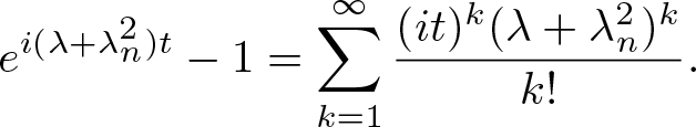 \begin{equation*}
e^{i(\lambda+\lambda_n^2)t}-1
=
\sum\limits_{k=1}^\infty
\frac{(it)^k(\lambda+\lambda_n^2)^k}{k!}.
\end{equation*}
\begin{equation*}
e^{i(\lambda+\lambda_n^2)t}-1
=
\sum\limits_{k=1}^\infty
\frac{(it)^k(\lambda+\lambda_n^2)^k}{k!}.
\end{equation*} Thus, we can write  $(5.38)\simeq\sum\limits_{k=1}^\infty \frac{i^{k}}{k!}f_k$, where
 \begin{align*}
f_k(r,t)
\doteq
t^k
\psi(t)\sum\limits_{0}^\infty
J_0(\lambda_n r)
\frac{1}{J_1(\lambda_n)}
\int_{-\infty}^0
e^{-i\lambda_n^2t}
\psi(\lambda+\lambda_n^2)(\lambda+\lambda_n^2)^{k-1}
\lambda_n
\widehat{h}(\lambda) d\lambda.
\end{align*}
\begin{align*}
f_k(r,t)
\doteq
t^k
\psi(t)\sum\limits_{0}^\infty
J_0(\lambda_n r)
\frac{1}{J_1(\lambda_n)}
\int_{-\infty}^0
e^{-i\lambda_n^2t}
\psi(\lambda+\lambda_n^2)(\lambda+\lambda_n^2)^{k-1}
\lambda_n
\widehat{h}(\lambda) d\lambda.
\end{align*}We can now estimate the weighted L 2-norm for this term, starting with the following
 \begin{align*}
\|r^{1/2}\cdot (5.38)\|_{L^2(0,1)}
\lesssim
\big\|
r^{1/2}\cdot
\sum\limits_{k=1}^\infty \frac{i^{k}}{k!}f_k
\big\|_{L^2(0,1)}
\lesssim
\sum\limits_{k=1}^\infty
\frac{1}{k!}
\|
r^{1/2}\cdot
f_k\|_{L^2(0,1)}.
\end{align*}
\begin{align*}
\|r^{1/2}\cdot (5.38)\|_{L^2(0,1)}
\lesssim
\big\|
r^{1/2}\cdot
\sum\limits_{k=1}^\infty \frac{i^{k}}{k!}f_k
\big\|_{L^2(0,1)}
\lesssim
\sum\limits_{k=1}^\infty
\frac{1}{k!}
\|
r^{1/2}\cdot
f_k\|_{L^2(0,1)}.
\end{align*} The Fourier–Bessel series coefficients for fk are given by  $
t^k\psi(t)e^{-i\lambda_n^2t}C_k(n),
$ where
$
t^k\psi(t)e^{-i\lambda_n^2t}C_k(n),
$ where
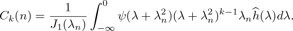 \begin{align*}
C_k(n)
=
\frac{1}{J_1(\lambda_n)}
\int_{-\infty}^0
\psi(\lambda+\lambda_n^2)(\lambda +\lambda_n^2)^{k-1}
\lambda_n
\widehat{h}(\lambda) d\lambda.
\end{align*}
\begin{align*}
C_k(n)
=
\frac{1}{J_1(\lambda_n)}
\int_{-\infty}^0
\psi(\lambda+\lambda_n^2)(\lambda +\lambda_n^2)^{k-1}
\lambda_n
\widehat{h}(\lambda) d\lambda.
\end{align*} Since ψ is compactly supported in  $(0,1)$, we can use Parseval’s identity (5.30) and Cauchy–Schwarz inequality to obtain
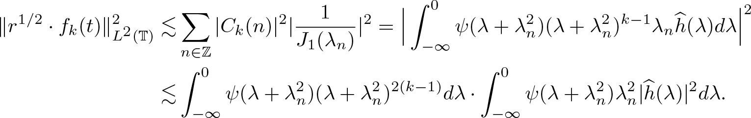 \begin{align*}
\|
r^{1/2}\cdot
f_k(t)\|_{L^2({\mathbb{T}})}^2
\lesssim&
\sum\limits_{n\in{\mathbb Z}}
|C_k(n)|^2
|\frac{1}{J_1(\lambda_n)}|^2
=
\Big|
\int_{-\infty}^0
\psi(\lambda+\lambda_n^2)(\lambda +\lambda_n^2)^{k-1}
\lambda_n
\widehat{h}(\lambda) d\lambda
\Big|^2
\\
\lesssim&
\int_{-\infty}^0
\psi(\lambda+\lambda_n^2)(\lambda +\lambda_n^2)^{2(k-1)}
d\lambda
\cdot
\int_{-\infty}^0
\psi(\lambda+\lambda_n^2)
\lambda_n^2
|\widehat{h}(\lambda)|^2 d\lambda.
\end{align*}
\begin{align*}
\|
r^{1/2}\cdot
f_k(t)\|_{L^2({\mathbb{T}})}^2
\lesssim&
\sum\limits_{n\in{\mathbb Z}}
|C_k(n)|^2
|\frac{1}{J_1(\lambda_n)}|^2
=
\Big|
\int_{-\infty}^0
\psi(\lambda+\lambda_n^2)(\lambda +\lambda_n^2)^{k-1}
\lambda_n
\widehat{h}(\lambda) d\lambda
\Big|^2
\\
\lesssim&
\int_{-\infty}^0
\psi(\lambda+\lambda_n^2)(\lambda +\lambda_n^2)^{2(k-1)}
d\lambda
\cdot
\int_{-\infty}^0
\psi(\lambda+\lambda_n^2)
\lambda_n^2
|\widehat{h}(\lambda)|^2 d\lambda.
\end{align*} Using the fact that  $\psi\in C^\infty_0(0,1)$, we can show that the first integral is bounded. For the second integral, note that $|\lambda+\lambda_n^2| \lt 1$, which implies that $\lambda_n^2\lesssim (1+|\lambda|)$. Therefore, we have
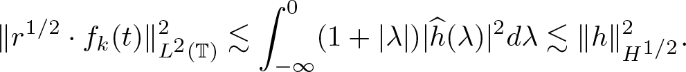 \begin{align*}
\|
r^{1/2}\cdot
f_k(t)\|_{L^2({\mathbb{T}})}^2
\lesssim
\int_{-\infty}^0
(1+|\lambda|)
|\widehat{h}(\lambda)|^2 d\lambda
\lesssim
\|h\|_{H^{1/2}}^2.
\end{align*}
\begin{align*}
\|
r^{1/2}\cdot
f_k(t)\|_{L^2({\mathbb{T}})}^2
\lesssim
\int_{-\infty}^0
(1+|\lambda|)
|\widehat{h}(\lambda)|^2 d\lambda
\lesssim
\|h\|_{H^{1/2}}^2.
\end{align*}This completes the desired estimate (5.28) for (5.38).
Proof of estimate (5.29). Using estimate (5.28), we prove this estimate for s = 0. Then, we will extend the proof to s = 2. We note that  $W_{ball} h$ defined by (5.27) satisfies the ibvp (5.12), which can be expressed as
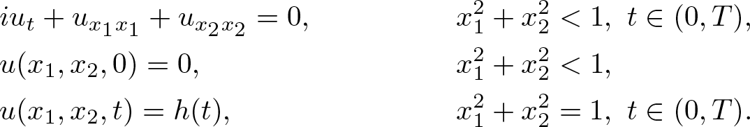 \begin{align*}
&iu_t+u_{x_1x_1} + u_{x_2x_2} =0,& & x_1^2 + x_2^2 \lt 1,\,\,t\in(0,T),
\\
&u(x_1, x_2 ,0)=0,& & x_1^2 + x_2^2 \lt 1,\\
&u(x_1, x_2 ,t)= h(t),&&x_1^2 + x_2^2 = 1, \,\, t\in(0,T).
\end{align*}
\begin{align*}
&iu_t+u_{x_1x_1} + u_{x_2x_2} =0,& & x_1^2 + x_2^2 \lt 1,\,\,t\in(0,T),
\\
&u(x_1, x_2 ,0)=0,& & x_1^2 + x_2^2 \lt 1,\\
&u(x_1, x_2 ,t)= h(t),&&x_1^2 + x_2^2 = 1, \,\, t\in(0,T).
\end{align*} If we let  $ u_t = v $, then $ v(x_1 , x_2, 0) = 0 $ and v satisfies the same ibvp with h replaced by ht, and we have
 \begin{align*}
\sup\limits_{t\in[0,T]}\Big\|
r^{1/2} v \Big\|_{L^2(0, 1)} =
\sup\limits_{t\in[0,T]}\Big\|
\big ( W_{ball} h
\big ) _t \Big\|_{L^2(\Omega_0)}
\le C_{T}
\|h_t \|_{H^{1/2}(0,T)}.
\end{align*}
\begin{align*}
\sup\limits_{t\in[0,T]}\Big\|
r^{1/2} v \Big\|_{L^2(0, 1)} =
\sup\limits_{t\in[0,T]}\Big\|
\big ( W_{ball} h
\big ) _t \Big\|_{L^2(\Omega_0)}
\le C_{T}
\|h_t \|_{H^{1/2}(0,T)}.
\end{align*} Hence, for a fixed value of t, the function  $u = W_{ball} h$ satisfies
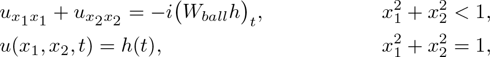 \begin{align*}
&u_{x_1x_1} + u_{x_2x_2} = - i \big ( W_{ball} h \big ) _t ,& & x_1^2 + x_2^2 \lt 1,
\\
&u(x_1, x_2 ,t)= h(t),&& x_1^2 + x_2^2 = 1,
\end{align*}
\begin{align*}
&u_{x_1x_1} + u_{x_2x_2} = - i \big ( W_{ball} h \big ) _t ,& & x_1^2 + x_2^2 \lt 1,
\\
&u(x_1, x_2 ,t)= h(t),&& x_1^2 + x_2^2 = 1,
\end{align*} which is an elliptic problem on Ω0. Since  $\big(W_{ball} h\big)_t \in L^2(\Omega_0)$ and h(t) is a constant for a fixed t, the theory of elliptic equations implies that $u \in H^2(\Omega_0)$ and
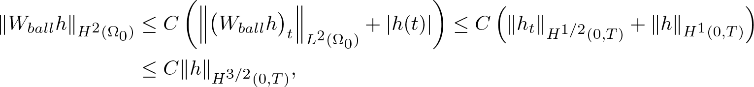 \begin{align*}
\| W_{ball }h \|_{H^2 (\Omega _0 ) } &\leq C \left (\Big\| \big ( W_{ball} h \big ) _t \Big\|_{L^2(\Omega_0)} + |h (t)| \right )
\leq C \left ( \|h_t \|_{H^{1/2}(0,T)} + \|h \|_{H^{1}(0,T)} \right )\\& \leq C \|h \|_{H^{3/2}(0,T)},
\end{align*}
\begin{align*}
\| W_{ball }h \|_{H^2 (\Omega _0 ) } &\leq C \left (\Big\| \big ( W_{ball} h \big ) _t \Big\|_{L^2(\Omega_0)} + |h (t)| \right )
\leq C \left ( \|h_t \|_{H^{1/2}(0,T)} + \|h \|_{H^{1}(0,T)} \right )\\& \leq C \|h \|_{H^{3/2}(0,T)},
\end{align*} where C is a constant dependent only on the domain Ω0. This completes the proof of estimate (5.29) for s = 2. The result for  $0 \lt s \lt 2$ follows from interpolation. Therefore, we complete the proof of proposition 5.4.
Now, we are able to state the linear estimate for the solution of ibvp (5.1). To do this, we first express the solution for this ibvp
 \begin{equation}
u
=
B[u_0,g; f]
\doteq
S_J[u_0;f]
+W_{ball}\big(
g
\big),
\quad
(x_1, x_2 ) \in \Omega_0,
\quad
t\in(0,T).
\end{equation}
\begin{equation}
u
=
B[u_0,g; f]
\doteq
S_J[u_0;f]
+W_{ball}\big(
g
\big),
\quad
(x_1, x_2 ) \in \Omega_0,
\quad
t\in(0,T).
\end{equation}Furthermore, using propositions 5.1 and 5.4, we obtain the linear estimate in the following solution spaces.
Theorem 5.6 Suppose that  $0\le s\leq 2$. If $u_0\in H^s_0(\Omega_0)$, $g\in H_{0}^{\frac{s+1}{2}}(0,T)$ (for $s=0,2$, $g\in H_{00}^{\frac{s+1}{2}}(0,T)$) and $f\in L^{1}\big(0,T; H^{s}_0(\Omega_0)\big)$, then $B[u_0, g_2; f]$ defines a solution to the linear ibvp (5.1) with compatibility condition (3.2), which satisfies
 \begin{align}
\sup\limits_{t\in[0,T]}\big\|B[u_0, g; f](t)\big\|_{H^s(\Omega_0)}
\lesssim
\|u_0\|_{H^s (\Omega_0)}
+
\|g \|_{H^{\frac{s+1}{2}}(0,T)}
+
\big\|f\big\|_{L^{1}\big(0,T; H^s (\Omega_0)\big)}.
\end{align}
\begin{align}
\sup\limits_{t\in[0,T]}\big\|B[u_0, g; f](t)\big\|_{H^s(\Omega_0)}
\lesssim
\|u_0\|_{H^s (\Omega_0)}
+
\|g \|_{H^{\frac{s+1}{2}}(0,T)}
+
\big\|f\big\|_{L^{1}\big(0,T; H^s (\Omega_0)\big)}.
\end{align}5.2. Nonlinear problem
We will now investigate the well-posedness of the nonlinear problem (1.1) for  $(x_1, x_2 ) \in \Omega_0$ with the boundary condition $u( x_1, x_2, t) = g (t )$ at $ x_1^2 + x_2^2 = 1$. In the solution formula (5.41), by replacing the forcing term f with $-\lambda|u|^{p-2}u$, we obtain the following iteration map
 \begin{equation}
u
=
B[u_0,g;f]
=
B[u_0,g ;-\lambda|u|^{p-2}u].
\end{equation}
\begin{equation}
u
=
B[u_0,g;f]
=
B[u_0,g ;-\lambda|u|^{p-2}u].
\end{equation}Remark. In (5.43), it is worth noting that for s > 1, we need the condition that  $f = -\lambda|u|^{p-2}u \in L^{1}\big(0,T; H^{s}_0(\Omega_0)\big)$. Thus, we can express (5.43) differently. Let
 \begin{equation*}
w(t)
=
-\lambda |u|^{p-2} u |_{x_1^2 + x_2^2 = 1}
=
-\lambda |g|^{p-2} g,
\end{equation*}
\begin{equation*}
w(t)
=
-\lambda |u|^{p-2} u |_{x_1^2 + x_2^2 = 1}
=
-\lambda |g|^{p-2} g,
\end{equation*} and  $v (t) = -i \int^t_0 w(s) ds$. Then, (5.43) can be transformed into the form
 \begin{align*}
u
= v(t) + B[u_0,g - v ; -\lambda|u|^{p-2}u - w ],
\end{align*}
\begin{align*}
u
= v(t) + B[u_0,g - v ; -\lambda|u|^{p-2}u - w ],
\end{align*} where  $-\lambda|u|^{p-2}u - w = 0$ at $x^2_1 + x_1^2 = 1$, which is the desired boundary condition. Here, v(t) is one order smoother than g if s > 1, which does not introduce any difficulties in deriving the relevant estimates. For the sake of simplicity, we will only consider (5.43) in the following.
Next, we will demonstrate that the iteration map defined by (5.43) is a contraction in the solution space  $C([0,T^*]; H^s (\Omega_0 ))$, for $1 \lt s \leq 2$. To do this, we can use the linear estimate (5.42) to obtain
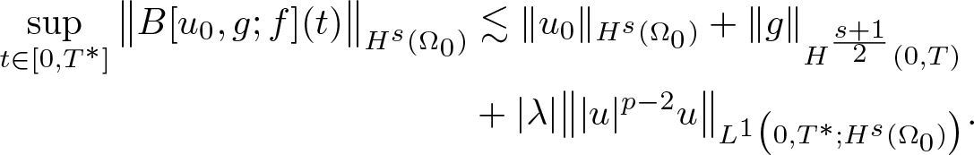 \begin{align*}
\sup\limits_{t\in[0,T^*]}\big\|B[u_0, g; f](t)\big\|_{H^s (\Omega_0 )}&
\lesssim
\|u_0\|_{H^s (\Omega_0 )}
+
\|g\|_{H^{\frac{s+1}{2}}(0,T)}\\&
+
|\lambda|\big\||u|^{p-2} u\big\|_{L^{1}\big(0,T^*; H^s (\Omega_0 )\big)}.
\end{align*}
\begin{align*}
\sup\limits_{t\in[0,T^*]}\big\|B[u_0, g; f](t)\big\|_{H^s (\Omega_0 )}&
\lesssim
\|u_0\|_{H^s (\Omega_0 )}
+
\|g\|_{H^{\frac{s+1}{2}}(0,T)}\\&
+
|\lambda|\big\||u|^{p-2} u\big\|_{L^{1}\big(0,T^*; H^s (\Omega_0 )\big)}.
\end{align*} To estimate the nonlinear term  $|u |^{p-2} u $, we extend u from $\Omega_0\times (0,T^*)$ to $\mathbb{R}^2 \times (0,T^*)$, such that the extension U satisfies
 \begin{equation*}
\|U\|_{L^{1}\big(0,T^*; H^s({\mathbb R}^2)\big)}
\le
2
\|u\|_{L^{1}\big(0,T^*; H^s (\Omega_0 )\big)}.
\end{equation*}
\begin{equation*}
\|U\|_{L^{1}\big(0,T^*; H^s({\mathbb R}^2)\big)}
\le
2
\|u\|_{L^{1}\big(0,T^*; H^s (\Omega_0 )\big)}.
\end{equation*} Hence, by applying Sobolev–Gagliardo–Nirenberg inequality (see [Reference Adams and Fournier1]) and Sobolev embedding theorem in  ${\mathbb R}^2$, for $s \gt \frac{2}{2}=1$ (if Ω0 is in $\mathbb R^n$, then $s \gt \frac n2$), we obtain
 \begin{align*}
\big\||u|^{p-2} u(t)\big\|_{ H^s (\Omega_0 )}
\lesssim
\big\||U|^{p-2} U(t)\big\|_{H^s({\mathbb R}^2)}
\overset{s \gt 1}{\le}
\|U(t)\|^{p-1}_{H^s({\mathbb R}^2)}
\lesssim
\|u(t)\|^{p-1}_{ H^s (\Omega_0 )}.
\end{align*}
\begin{align*}
\big\||u|^{p-2} u(t)\big\|_{ H^s (\Omega_0 )}
\lesssim
\big\||U|^{p-2} U(t)\big\|_{H^s({\mathbb R}^2)}
\overset{s \gt 1}{\le}
\|U(t)\|^{p-1}_{H^s({\mathbb R}^2)}
\lesssim
\|u(t)\|^{p-1}_{ H^s (\Omega_0 )}.
\end{align*}Working similarly, for s > 1, we get
 \begin{align*}
\big\||u|^{p-2} u(t)-|v|^{p-2} v(t)\big\|_{H^s (\Omega_0 )}
\lesssim
\big(
\|u(t)\|_{ H^s (\Omega_0 )}^{p-2}+\|v(t)\|_{ H^s (\Omega_0 ) }^{p-2}
\big)
\|(u-v)(t)\|_{ H^s (\Omega_0 ) }.
\end{align*}
\begin{align*}
\big\||u|^{p-2} u(t)-|v|^{p-2} v(t)\big\|_{H^s (\Omega_0 )}
\lesssim
\big(
\|u(t)\|_{ H^s (\Omega_0 )}^{p-2}+\|v(t)\|_{ H^s (\Omega_0 ) }^{p-2}
\big)
\|(u-v)(t)\|_{ H^s (\Omega_0 ) }.
\end{align*}Finally, using Hölder’s inequality in t integral, we arrive at
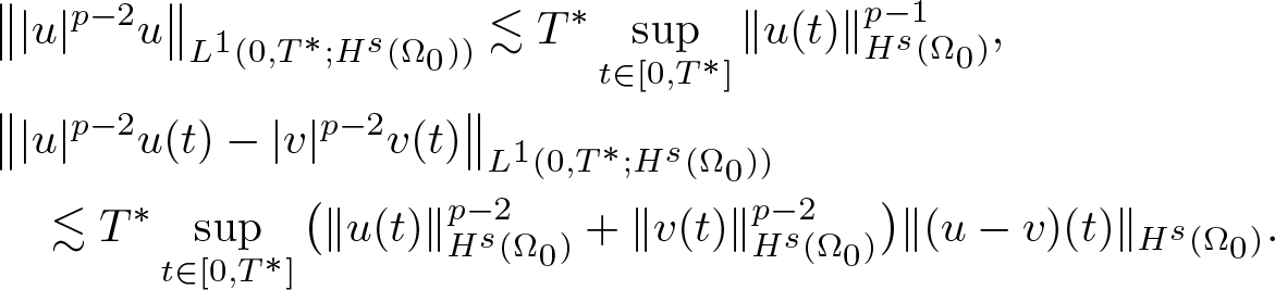 \begin{align*}
&\big\||u|^{p-2} u\big\|_{L^1(0,T^*; H^s (\Omega_0 ))}
\lesssim
T^*\sup\limits_{t\in [0,T^*]}
\|u(t)\|^{p-1}_{ H^s (\Omega_0 )},
\\
&\big\||u|^{p-2} u(t)-|v|^{p-2} v(t)\big\|_{L^1(0,T^*; H^s (\Omega_0 ))}\\ &\quad
\lesssim
T^*\sup\limits_{t\in [0,T^*]}
\big(
\|u(t)\|_{ H^s (\Omega_0 ) }^{p-2}+\|v(t)\|_{ H^s (\Omega_0 ) }^{p-2}
\big)
\|(u-v)(t)\|_{ H^s (\Omega_0 )}.
\end{align*}
\begin{align*}
&\big\||u|^{p-2} u\big\|_{L^1(0,T^*; H^s (\Omega_0 ))}
\lesssim
T^*\sup\limits_{t\in [0,T^*]}
\|u(t)\|^{p-1}_{ H^s (\Omega_0 )},
\\
&\big\||u|^{p-2} u(t)-|v|^{p-2} v(t)\big\|_{L^1(0,T^*; H^s (\Omega_0 ))}\\ &\quad
\lesssim
T^*\sup\limits_{t\in [0,T^*]}
\big(
\|u(t)\|_{ H^s (\Omega_0 ) }^{p-2}+\|v(t)\|_{ H^s (\Omega_0 ) }^{p-2}
\big)
\|(u-v)(t)\|_{ H^s (\Omega_0 )}.
\end{align*} Using the above estimates, we find that the iteration map (5.43) is a contraction in  $C([0,T^*]; H^s (\Omega_0 ))$ for s > 1, as long as $T^* \gt 0$ is sufficiently small. Thus, we obtain a unique solution $u \in C ([0,T^*]; H^s (\Omega_0 ))$. Given the radial symmetry of the initial and boundary conditions, and due to the uniqueness and rotational invariance of this problem, the solution is also radially symmetric. Consequently, u is a function of $r = \sqrt {x_1^2 + x_2^2}$ in terms of spatial variables.
Funding
The first author was partially supported by a grant from the Simons Foundation (712822, SMS).
Appendix A
Proof of estimate (3.32). We define theoperator  $J: L^2\to L_t^q({\mathbb R}; L^{\gamma}(1,\infty))$ as follows
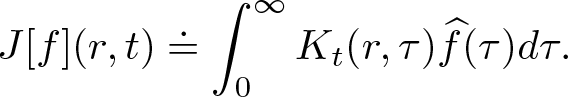 \begin{equation}
J[f](r,t)
\doteq
\int_0^\infty
K_t(r,\tau)
\widehat{f}(\tau)
d\tau.
\end{equation}
\begin{equation}
J[f](r,t)
\doteq
\int_0^\infty
K_t(r,\tau)
\widehat{f}(\tau)
d\tau.
\end{equation}To establish estimate (3.32), it suffices to demonstrate that J is bounded. To do this, we will show that the adjoint operator of J is bounded. Utilizing duality, we have
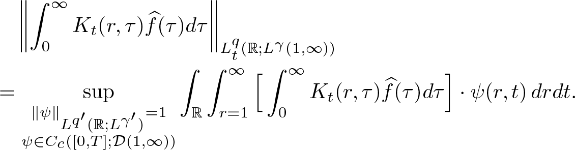 \begin{align*}
&\quad \left \|
\int_0^\infty
K_t(r,\tau)
\widehat{f}(\tau)
d\tau
\right \|_{L_t^q({\mathbb R}; L^{\gamma}(1,\infty))}\\&
=
\sup\limits_{\substack{\|\psi\|_{L^{q'}({\mathbb R}; L^{\gamma'})}=1\\ \psi
\in
C_c([0,T]; \mathcal{D}(1,\infty))}}
\int_{{\mathbb R}}
\int_{r=1}^\infty
\Big[
\int_0^\infty
K_t(r,\tau)
\widehat{f}(\tau)
d\tau
\Big]
\cdot
\psi
(r,t)
\,
dr
dt.
\end{align*}
\begin{align*}
&\quad \left \|
\int_0^\infty
K_t(r,\tau)
\widehat{f}(\tau)
d\tau
\right \|_{L_t^q({\mathbb R}; L^{\gamma}(1,\infty))}\\&
=
\sup\limits_{\substack{\|\psi\|_{L^{q'}({\mathbb R}; L^{\gamma'})}=1\\ \psi
\in
C_c([0,T]; \mathcal{D}(1,\infty))}}
\int_{{\mathbb R}}
\int_{r=1}^\infty
\Big[
\int_0^\infty
K_t(r,\tau)
\widehat{f}(\tau)
d\tau
\Big]
\cdot
\psi
(r,t)
\,
dr
dt.
\end{align*} Now, utilizing (3.31), we obtain the t-Fourier transform of  $\int_0^\infty K_t(r,\tau) \widehat{f}(\tau) d\tau$, which is
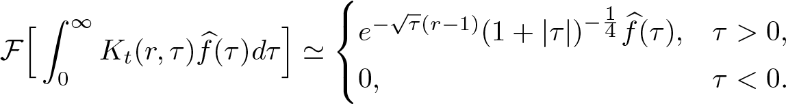 \begin{equation*}
\mathcal{F}
\Big[
\int_0^\infty
K_t(r,\tau)
\widehat{f}(\tau)
d\tau
\Big]
\simeq
\begin{cases}
e^{-\sqrt{\tau} (r-1)}
(1+|\tau|)^{-\frac14}
\widehat{f}(\tau),
\quad
&\tau \gt 0,
\\
0,
\quad
&\tau \lt 0.
\end{cases}
\end{equation*}
\begin{equation*}
\mathcal{F}
\Big[
\int_0^\infty
K_t(r,\tau)
\widehat{f}(\tau)
d\tau
\Big]
\simeq
\begin{cases}
e^{-\sqrt{\tau} (r-1)}
(1+|\tau|)^{-\frac14}
\widehat{f}(\tau),
\quad
&\tau \gt 0,
\\
0,
\quad
&\tau \lt 0.
\end{cases}
\end{equation*}Combined with the Plancherel theorem, we obtain
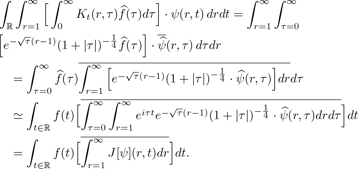 \begin{align*}
&\int_{{\mathbb R}}
\int_{r=1}^\infty
\Big[
\int_0^\infty
K_t(r,\tau)
\widehat{f}(\tau)
d\tau
\Big]
\cdot
\psi
(r,t)
\,
dr
dt
=
\int_{r=1}^\infty
\int_{\tau=0}^\infty
\\&
\Big[
e^{-\sqrt{\tau} (r-1)}
(1+|\tau|)^{-\frac14}
\widehat{f}(\tau)
\Big]
\cdot
\overline{\widehat{\psi}}
(r,\tau)
\,
d\tau
dr
\\
& \quad =
\int_{\tau=0}^\infty
\widehat{f}(\tau)
\overline{
\int_{r=1}^\infty
\Big[
e^{-\sqrt{\tau} (r-1)}
(1+|\tau|)^{-\frac14}
\cdot
\widehat{\psi}
(r,\tau)
\Big]
dr
}
d\tau
\\
& \quad
\simeq
\int_{t\in{\mathbb R}}
f(t)
\Big[
\overline{
\int_{\tau=0}^\infty
\int_{r=1}^\infty
e^{i\tau t}
e^{-\sqrt{\tau} (r-1)}
(1+|\tau|)^{-\frac14}
\cdot
\widehat{\psi}
(r,\tau)
dr
d\tau
}
\Big]
dt
\\
& \quad
=
\int_{t\in{\mathbb R}}
f(t)
\Big[
\overline{
\int_{r=1}^\infty
J[\psi](r,t)
dr
}
\Big]
dt.
\end{align*}
\begin{align*}
&\int_{{\mathbb R}}
\int_{r=1}^\infty
\Big[
\int_0^\infty
K_t(r,\tau)
\widehat{f}(\tau)
d\tau
\Big]
\cdot
\psi
(r,t)
\,
dr
dt
=
\int_{r=1}^\infty
\int_{\tau=0}^\infty
\\&
\Big[
e^{-\sqrt{\tau} (r-1)}
(1+|\tau|)^{-\frac14}
\widehat{f}(\tau)
\Big]
\cdot
\overline{\widehat{\psi}}
(r,\tau)
\,
d\tau
dr
\\
& \quad =
\int_{\tau=0}^\infty
\widehat{f}(\tau)
\overline{
\int_{r=1}^\infty
\Big[
e^{-\sqrt{\tau} (r-1)}
(1+|\tau|)^{-\frac14}
\cdot
\widehat{\psi}
(r,\tau)
\Big]
dr
}
d\tau
\\
& \quad
\simeq
\int_{t\in{\mathbb R}}
f(t)
\Big[
\overline{
\int_{\tau=0}^\infty
\int_{r=1}^\infty
e^{i\tau t}
e^{-\sqrt{\tau} (r-1)}
(1+|\tau|)^{-\frac14}
\cdot
\widehat{\psi}
(r,\tau)
dr
d\tau
}
\Big]
dt
\\
& \quad
=
\int_{t\in{\mathbb R}}
f(t)
\Big[
\overline{
\int_{r=1}^\infty
J[\psi](r,t)
dr
}
\Big]
dt.
\end{align*}Thus, the adjoint operator of J is given by
 \begin{equation}
J^*[\psi](t)
\doteq
\overline{
\int_{r=1}^\infty
J[\psi](r,t)
dr
}.
\end{equation}
\begin{equation}
J^*[\psi](t)
\doteq
\overline{
\int_{r=1}^\infty
J[\psi](r,t)
dr
}.
\end{equation}Furthermore, using the Hölder inequality, to establish that J is bounded, it suffices to show
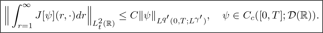 \begin{equation}
\boxed{
\Big\|
\int_{r=1}^\infty
J[\psi](r,\cdot)
dr
\Big\|_{L^2_t({\mathbb R})}
\le
C
\|\psi\|_{L^{q'}(0,T; L^{\gamma'})},
\quad
\psi
\in
C_c([0,T]; \mathcal{D}({\mathbb R})).
}
\end{equation}
\begin{equation}
\boxed{
\Big\|
\int_{r=1}^\infty
J[\psi](r,\cdot)
dr
\Big\|_{L^2_t({\mathbb R})}
\le
C
\|\psi\|_{L^{q'}(0,T; L^{\gamma'})},
\quad
\psi
\in
C_c([0,T]; \mathcal{D}({\mathbb R})).
}
\end{equation}We have
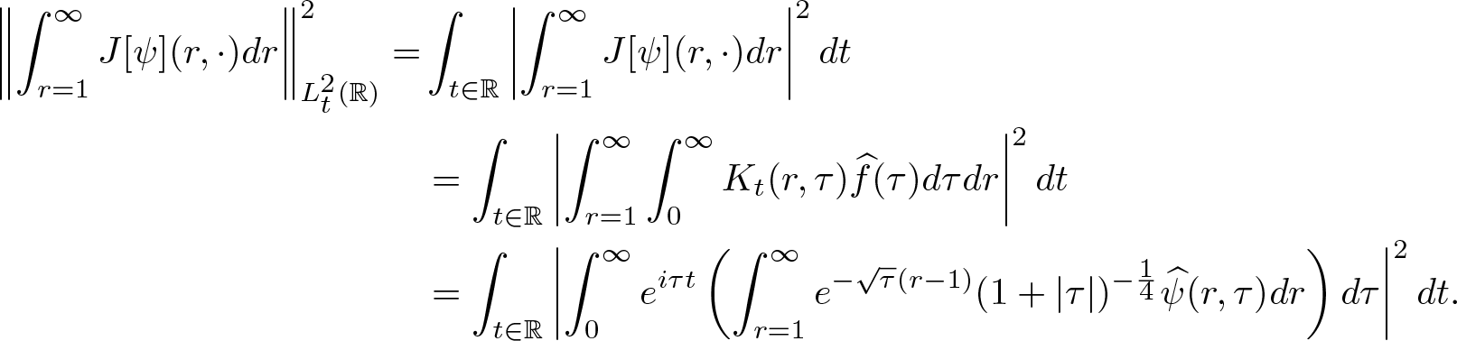 \begin{align*}
\left\|
\int_{r=1}^\infty
J[\psi](r,\cdot)
dr
\right\|_{L_t^2({\mathbb R})}^2
=&
\int_{t\in{\mathbb R}}\left|
\int_{r=1}^\infty
J[\psi](r,\cdot)
dr
\right|^2dt\\&
=
\int_{t\in{\mathbb R}}\left|\int_{r=1}^{\infty}
\int_0^\infty
K_t(r,\tau)
\widehat{f}(\tau)
d\tau
dr
\right|^2dt
\nonumber
\\&
=
\int_{t\in{\mathbb R}}\left|\int_{0}^\infty e^{i\tau t}
\left(\int_{r=1}^{\infty}
e^{-\sqrt{\tau} (r-1)}
(1+|\tau|)^{-\frac14}
\widehat{\psi}(r,\tau)
dr\right)d\tau\right|^2dt.
\end{align*}
\begin{align*}
\left\|
\int_{r=1}^\infty
J[\psi](r,\cdot)
dr
\right\|_{L_t^2({\mathbb R})}^2
=&
\int_{t\in{\mathbb R}}\left|
\int_{r=1}^\infty
J[\psi](r,\cdot)
dr
\right|^2dt\\&
=
\int_{t\in{\mathbb R}}\left|\int_{r=1}^{\infty}
\int_0^\infty
K_t(r,\tau)
\widehat{f}(\tau)
d\tau
dr
\right|^2dt
\nonumber
\\&
=
\int_{t\in{\mathbb R}}\left|\int_{0}^\infty e^{i\tau t}
\left(\int_{r=1}^{\infty}
e^{-\sqrt{\tau} (r-1)}
(1+|\tau|)^{-\frac14}
\widehat{\psi}(r,\tau)
dr\right)d\tau\right|^2dt.
\end{align*}Applying Plancherel theorem to dt, we have
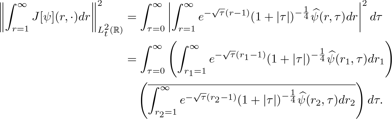 \begin{align*}
\left\|
\int_{r=1}^\infty
J[\psi](r,\cdot)
dr
\right\|_{L_t^2({\mathbb R})}^2&
=
\int_{\tau=0}^\infty
\left|\int_{r=1}^{\infty}
e^{-\sqrt{\tau} (r-1)}
(1+|\tau|)^{-\frac14}
\widehat{\psi}(r,\tau)
dr
\right|^2
d\tau\\&
=
\int_{\tau=0}^\infty
\left(
\int_{r_1=1}^\infty
e^{-\sqrt{\tau} (r_1-1)}
(1+|\tau|)^{-\frac14}
\widehat{\psi}(r_1,\tau)
dr_1
\right)\\&\quad
\left(
\overline{\int_{r_2=1}^\infty
e^{-\sqrt{\tau} (r_2-1)}
(1+|\tau|)^{-\frac14}
\widehat{\psi}(r_2,\tau)
dr_2
}
\right)
d\tau.
\nonumber
\end{align*}
\begin{align*}
\left\|
\int_{r=1}^\infty
J[\psi](r,\cdot)
dr
\right\|_{L_t^2({\mathbb R})}^2&
=
\int_{\tau=0}^\infty
\left|\int_{r=1}^{\infty}
e^{-\sqrt{\tau} (r-1)}
(1+|\tau|)^{-\frac14}
\widehat{\psi}(r,\tau)
dr
\right|^2
d\tau\\&
=
\int_{\tau=0}^\infty
\left(
\int_{r_1=1}^\infty
e^{-\sqrt{\tau} (r_1-1)}
(1+|\tau|)^{-\frac14}
\widehat{\psi}(r_1,\tau)
dr_1
\right)\\&\quad
\left(
\overline{\int_{r_2=1}^\infty
e^{-\sqrt{\tau} (r_2-1)}
(1+|\tau|)^{-\frac14}
\widehat{\psi}(r_2,\tau)
dr_2
}
\right)
d\tau.
\nonumber
\end{align*}Using Fubini’s theorem, we can simplify the expression to
 \begin{align*}
\left\|
\int_{r=1}^\infty
J[\psi](r,\cdot)
dr
\right\|_{L_t^2({\mathbb R})}^2&
=
\int_{r_1=1}^\infty \int_{\tau=0}^\infty\widehat{\psi}(r_1,\tau)\\ &\quad
\left(
\overline{\int_{r_2=1}^\infty
e^{-\sqrt{\tau} (r_1+r_2-2)}
(1+|\tau|)^{-\frac12}
\widehat{\psi}(r_2,\tau)
dr_2}
\right)
d\tau dr_1.
\end{align*}
\begin{align*}
\left\|
\int_{r=1}^\infty
J[\psi](r,\cdot)
dr
\right\|_{L_t^2({\mathbb R})}^2&
=
\int_{r_1=1}^\infty \int_{\tau=0}^\infty\widehat{\psi}(r_1,\tau)\\ &\quad
\left(
\overline{\int_{r_2=1}^\infty
e^{-\sqrt{\tau} (r_1+r_2-2)}
(1+|\tau|)^{-\frac12}
\widehat{\psi}(r_2,\tau)
dr_2}
\right)
d\tau dr_1.
\end{align*} Furthermore, applying Plancherel’s theorem to  $d\tau$, we have
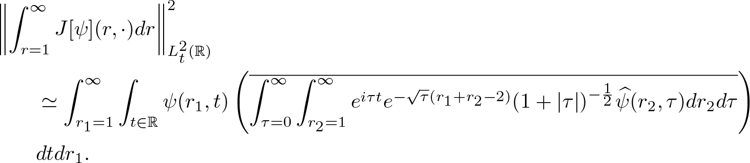 \begin{align*}
& \left\|
\int_{r=1}^\infty
J[\psi](r,\cdot)
dr
\right\|_{L_t^2({\mathbb R})}^2\\
&\qquad
\simeq
\int_{r_1=1}^\infty\int_{t\in{\mathbb R}}\psi(r_1,t)
\left(
\overline{\int_{\tau=0}^\infty\int_{r_2=1}^\infty
e^{i\tau t}
e^{-\sqrt{\tau} (r_1+r_2-2)}
(1+|\tau|)^{-\frac12}
\widehat{\psi}(r_2,\tau)
dr_2 d\tau}
\right)\\& \quad \quad
dt dr_1.
\end{align*}
\begin{align*}
& \left\|
\int_{r=1}^\infty
J[\psi](r,\cdot)
dr
\right\|_{L_t^2({\mathbb R})}^2\\
&\qquad
\simeq
\int_{r_1=1}^\infty\int_{t\in{\mathbb R}}\psi(r_1,t)
\left(
\overline{\int_{\tau=0}^\infty\int_{r_2=1}^\infty
e^{i\tau t}
e^{-\sqrt{\tau} (r_1+r_2-2)}
(1+|\tau|)^{-\frac12}
\widehat{\psi}(r_2,\tau)
dr_2 d\tau}
\right)\\& \quad \quad
dt dr_1.
\end{align*}Moreover, applying Holder’s inequality to dr 1 and dt, we get
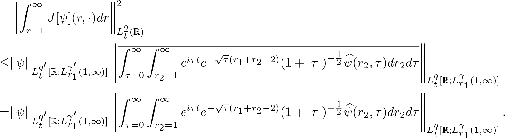 \begin{align*}
&\left\|
\int_{r=1}^\infty
J[\psi](r,\cdot)
dr
\right\|_{L_t^2({\mathbb R})}^2
\nonumber
\\
\leq&
\|\psi\|_{L_t^{q'}[{\mathbb R};L_{r_1}^{\gamma'}(1,\infty)]}
\left\|
\overline{\int_{\tau=0}^\infty\int_{r_2=1}^\infty
e^{i\tau t}
e^{-\sqrt{\tau} (r_1+r_2-2)}
(1+|\tau|)^{-\frac12}
\widehat{\psi}(r_2,\tau)
dr_2 d\tau}
\right\|_{L_t^{q}[{\mathbb R};L_{r_1}^{\gamma}(1,\infty)]}
\nonumber
\\
=&
\|\psi \|_{L_t^{q'}[{\mathbb R};L_{r_1}^{\gamma'}(1,\infty)]}
\left\|
\int_{\tau=0}^\infty\int_{r_2=1}^\infty
e^{i\tau t}
e^{-\sqrt{\tau} (r_1+r_2-2)}
(1+|\tau|)^{-\frac12}
\widehat{\psi}(r_2,\tau)
dr_2 d\tau
\right\|_{L_t^{q}[{\mathbb R};L_{r_1}^{\gamma}(1,\infty)]}.
\end{align*}
\begin{align*}
&\left\|
\int_{r=1}^\infty
J[\psi](r,\cdot)
dr
\right\|_{L_t^2({\mathbb R})}^2
\nonumber
\\
\leq&
\|\psi\|_{L_t^{q'}[{\mathbb R};L_{r_1}^{\gamma'}(1,\infty)]}
\left\|
\overline{\int_{\tau=0}^\infty\int_{r_2=1}^\infty
e^{i\tau t}
e^{-\sqrt{\tau} (r_1+r_2-2)}
(1+|\tau|)^{-\frac12}
\widehat{\psi}(r_2,\tau)
dr_2 d\tau}
\right\|_{L_t^{q}[{\mathbb R};L_{r_1}^{\gamma}(1,\infty)]}
\nonumber
\\
=&
\|\psi \|_{L_t^{q'}[{\mathbb R};L_{r_1}^{\gamma'}(1,\infty)]}
\left\|
\int_{\tau=0}^\infty\int_{r_2=1}^\infty
e^{i\tau t}
e^{-\sqrt{\tau} (r_1+r_2-2)}
(1+|\tau|)^{-\frac12}
\widehat{\psi}(r_2,\tau)
dr_2 d\tau
\right\|_{L_t^{q}[{\mathbb R};L_{r_1}^{\gamma}(1,\infty)]}.
\end{align*}Now, to prove the inequality (A.3), it is enough to show that
 \begin{align}
& \boxed{
\left\|
\int_{\tau=0}^\infty\int_{r_2=1}^\infty
e^{i\tau t}
e^{-\sqrt{\tau} (r_1+r_2-2)}
(1+|\tau|)^{-\frac12}
\widehat{\psi}(r_2,\tau)
dr_2 d\tau
\right\|_{L_t^{q}[{\mathbb R};L_{r_1}^{\gamma}(1,\infty)]}}\nonumber\\&\quad
\boxed{\lesssim
\|\psi\|_{L_t^{q'}[{\mathbb R};L^{\gamma'}(1,\infty)]}.
}
\end{align}
\begin{align}
& \boxed{
\left\|
\int_{\tau=0}^\infty\int_{r_2=1}^\infty
e^{i\tau t}
e^{-\sqrt{\tau} (r_1+r_2-2)}
(1+|\tau|)^{-\frac12}
\widehat{\psi}(r_2,\tau)
dr_2 d\tau
\right\|_{L_t^{q}[{\mathbb R};L_{r_1}^{\gamma}(1,\infty)]}}\nonumber\\&\quad
\boxed{\lesssim
\|\psi\|_{L_t^{q'}[{\mathbb R};L^{\gamma'}(1,\infty)]}.
}
\end{align} To proceed, we will use the convolution property:  $
\mathcal{F}^{-1}(f\cdot g)
=
\mathcal{F}^{-1}(g)*
\mathcal{F}^{-1}(g).
$ This allows us to rewrite the integral as
$
\mathcal{F}^{-1}(f\cdot g)
=
\mathcal{F}^{-1}(g)*
\mathcal{F}^{-1}(g).
$ This allows us to rewrite the integral as
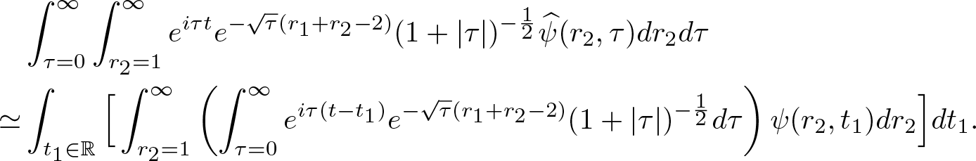 \begin{align*}
&
\int_{\tau=0}^\infty
\int_{r_2=1}^\infty
e^{i\tau t}
e^{-\sqrt{\tau} (r_1+r_2-2)}
(1+|\tau|)^{-\frac12}
\widehat{\psi}(r_2,\tau)
dr_2 d\tau
\\
\simeq&
\int_{t_1\in{\mathbb R}}
\Big[
\int_{r_2=1}^\infty
\left(
\int_{\tau=0}^\infty
e^{i\tau (t-t_1)}
e^{-\sqrt{\tau} (r_1+r_2-2)}
(1+|\tau|)^{-\frac12}
d\tau
\right)
\psi(r_2,t_1)
dr_2
\Big]
dt_1.
\end{align*}
\begin{align*}
&
\int_{\tau=0}^\infty
\int_{r_2=1}^\infty
e^{i\tau t}
e^{-\sqrt{\tau} (r_1+r_2-2)}
(1+|\tau|)^{-\frac12}
\widehat{\psi}(r_2,\tau)
dr_2 d\tau
\\
\simeq&
\int_{t_1\in{\mathbb R}}
\Big[
\int_{r_2=1}^\infty
\left(
\int_{\tau=0}^\infty
e^{i\tau (t-t_1)}
e^{-\sqrt{\tau} (r_1+r_2-2)}
(1+|\tau|)^{-\frac12}
d\tau
\right)
\psi(r_2,t_1)
dr_2
\Big]
dt_1.
\end{align*}Additionally, following a similar approach to the proof in reference [Reference Bona, Sun and Zhang7], we obtain
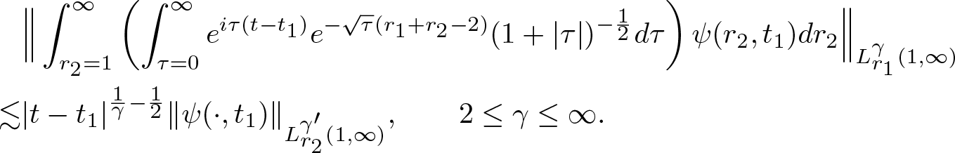 \begin{align}
&\Big\|
\int_{r_2=1}^\infty
\left(
\int_{\tau=0}^\infty
e^{i\tau (t-t_1)}
e^{-\sqrt{\tau} (r_1+r_2-2)}
(1+|\tau|)^{-\frac12}
d\tau
\right)
\psi(r_2,t_1)
dr_2
\Big\|_{L_{r_1}^{\gamma}(1,\infty)}
\nonumber
\\
\lesssim&
|t-t_1|^{\frac1\gamma-\frac12}
\|\psi(\cdot,t_1)\|_{L_{r_2}^{\gamma'}(1,\infty)},
\qquad
2\le \gamma \le \infty.
\end{align}
\begin{align}
&\Big\|
\int_{r_2=1}^\infty
\left(
\int_{\tau=0}^\infty
e^{i\tau (t-t_1)}
e^{-\sqrt{\tau} (r_1+r_2-2)}
(1+|\tau|)^{-\frac12}
d\tau
\right)
\psi(r_2,t_1)
dr_2
\Big\|_{L_{r_1}^{\gamma}(1,\infty)}
\nonumber
\\
\lesssim&
|t-t_1|^{\frac1\gamma-\frac12}
\|\psi(\cdot,t_1)\|_{L_{r_2}^{\gamma'}(1,\infty)},
\qquad
2\le \gamma \le \infty.
\end{align}Finally, we combine the above estimate with the following result to obtain the desired estimate (A.6).
Lemma A.1. Hardy–Littlewood–Polya [Reference Hardy, Littlewood and Pólya26] section 10.17, theorem 382
If  $F,G\geq 0$ then
 \begin{align}
\int_{{\mathbb R}}\int_{{\mathbb R}}\frac{F(x)G(y)}{|x-y|^\lambda}dxdy
\leq
C\|F\|_{L_x^P({\mathbb R})}\|G\|_{L_x^Q({\mathbb R})},
\quad
C \gt 0,
\end{align}
\begin{align}
\int_{{\mathbb R}}\int_{{\mathbb R}}\frac{F(x)G(y)}{|x-y|^\lambda}dxdy
\leq
C\|F\|_{L_x^P({\mathbb R})}\|G\|_{L_x^Q({\mathbb R})},
\quad
C \gt 0,
\end{align} with  $P \gt 1, Q \gt 1$, $\frac{1}{P}+\frac{1}{Q} \gt 1$, $\lambda=2-\frac{1}{P}-\frac{1}{Q}$.
It can be observed that
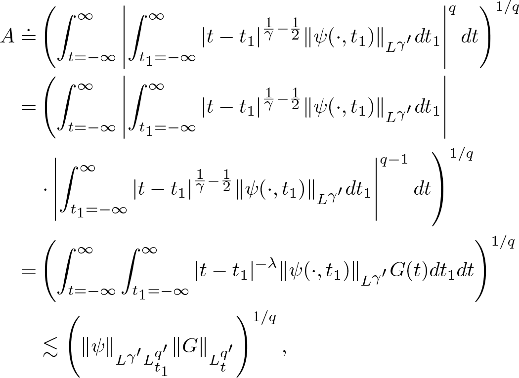 \begin{align*}
A
\doteq
&\left(
\int_{t=-\infty}^\infty\left|\int_{t_1=-\infty}^\infty
|t-t_1|^{\frac1\gamma-\frac12}\|\psi(\cdot,t_1)\|_{L^{\gamma'}}
dt_1
\right|^qdt
\right)^{1/q}
\\
=&
\left(
\int_{t=-\infty}^\infty
\left|\int_{t_1=-\infty}^\infty
|t-t_1|^{\frac1\gamma-\frac12}\|\psi(\cdot,t_1)\|_{L^{\gamma'}}
dt_1
\right| \right. \\& \left.
\cdot
\left|\int_{t_1=-\infty}^\infty
|t-t_1|^{\frac1\gamma-\frac12}\|\psi(\cdot,t_1)\|_{L^{\gamma'}}
dt_1
\right|^{q-1}dt
\right)^{1/q}
\\
=&
\left(
\int_{t=-\infty}^\infty
\int_{t_1=-\infty}^\infty
|t-t_1|^{-\lambda}\|\psi(\cdot,t_1)\|_{L^{\gamma'}}
G(t)dt_1 dt
\right)^{1/q}\\&
\lesssim
\left(
\|\psi\|_{L^{\gamma'}L_{t_1}^{q'}}\|G\|_{L_t^{q'}}
\right)^{1/q},
\end{align*}
\begin{align*}
A
\doteq
&\left(
\int_{t=-\infty}^\infty\left|\int_{t_1=-\infty}^\infty
|t-t_1|^{\frac1\gamma-\frac12}\|\psi(\cdot,t_1)\|_{L^{\gamma'}}
dt_1
\right|^qdt
\right)^{1/q}
\\
=&
\left(
\int_{t=-\infty}^\infty
\left|\int_{t_1=-\infty}^\infty
|t-t_1|^{\frac1\gamma-\frac12}\|\psi(\cdot,t_1)\|_{L^{\gamma'}}
dt_1
\right| \right. \\& \left.
\cdot
\left|\int_{t_1=-\infty}^\infty
|t-t_1|^{\frac1\gamma-\frac12}\|\psi(\cdot,t_1)\|_{L^{\gamma'}}
dt_1
\right|^{q-1}dt
\right)^{1/q}
\\
=&
\left(
\int_{t=-\infty}^\infty
\int_{t_1=-\infty}^\infty
|t-t_1|^{-\lambda}\|\psi(\cdot,t_1)\|_{L^{\gamma'}}
G(t)dt_1 dt
\right)^{1/q}\\&
\lesssim
\left(
\|\psi\|_{L^{\gamma'}L_{t_1}^{q'}}\|G\|_{L_t^{q'}}
\right)^{1/q},
\end{align*} where we have taken  $\lambda=\frac12-\frac1\gamma$, $G(t)=\left|\int_{t_1=-\infty}^\infty |t-t_1|^{\frac1\gamma-\frac12}|\psi(\cdot,t_1)|_{L^{\gamma'}}dt_1\right|^{q-1}$, and set $P=Q=q'$. It is easy to verify that the admissible condition $\frac{2}{q}+\frac{1}{\gamma}=\frac12$ implies that $\lambda=2-\frac1P-\frac1Q$. In fact, we have
 \begin{equation*}
\lambda=\frac12-\frac1\gamma
=
\frac12-(\frac12-\frac2q)
=
\frac2q
=
2-\frac2{q'}
=
2-\frac1P-\frac1Q.
\end{equation*}
\begin{equation*}
\lambda=\frac12-\frac1\gamma
=
\frac12-(\frac12-\frac2q)
=
\frac2q
=
2-\frac2{q'}
=
2-\frac1P-\frac1Q.
\end{equation*}Additionally, we have
 \begin{align*}
\|G\|_{L_t^{q'}({\mathbb R})}
=
\left(\int_{t\in{\mathbb R}}\left|\int_{t_1=-\infty}^\infty
|t-t_1|^{\frac1\gamma-\frac12}\|\psi(\cdot,t_1)\|_{L^{\gamma'}}
dt_1
\right|^{(q-1)q'}
dt
\right)^{1/q'}.
\end{align*}
\begin{align*}
\|G\|_{L_t^{q'}({\mathbb R})}
=
\left(\int_{t\in{\mathbb R}}\left|\int_{t_1=-\infty}^\infty
|t-t_1|^{\frac1\gamma-\frac12}\|\psi(\cdot,t_1)\|_{L^{\gamma'}}
dt_1
\right|^{(q-1)q'}
dt
\right)^{1/q'}.
\end{align*} Combining the above identity with  $\frac{1}{q'}=1-\frac{1}{q}$, or $q'=\frac{q}{q-1}$, we get
 \begin{align*}
\|G\|_{L_t^{q'}({\mathbb R})}
=
\left(\int_{t\in{\mathbb R}}\left|\int_{t_1=-\infty}^\infty
|t-t_1|^{\frac1\gamma-\frac12}\|\psi(\cdot,t_1)\|_{L^{\gamma'}}
dt_1
\right|^{q}
dt
\right)^{1/q'}
=
A^{q/q'}\, .
\end{align*}
\begin{align*}
\|G\|_{L_t^{q'}({\mathbb R})}
=
\left(\int_{t\in{\mathbb R}}\left|\int_{t_1=-\infty}^\infty
|t-t_1|^{\frac1\gamma-\frac12}\|\psi(\cdot,t_1)\|_{L^{\gamma'}}
dt_1
\right|^{q}
dt
\right)^{1/q'}
=
A^{q/q'}\, .
\end{align*}Thus, we find
 \begin{align*}
A
\lesssim
\left(
\|\psi\|_{L^{\gamma'}L_{t_1}^{q'}}\|G\|_{L_t^{q'}({\mathbb R})}
\right)^{1/q}
=
\left(
\|\psi\|_{L^{\gamma'}L_{t_1}^{q'}}A^{q/q'}
\right)^{1/q}
=
\|\psi\|_{L^{\gamma'}L_{t_1}^{q'}}^{1/q}A^{1/q'}\, .
\end{align*}
\begin{align*}
A
\lesssim
\left(
\|\psi\|_{L^{\gamma'}L_{t_1}^{q'}}\|G\|_{L_t^{q'}({\mathbb R})}
\right)^{1/q}
=
\left(
\|\psi\|_{L^{\gamma'}L_{t_1}^{q'}}A^{q/q'}
\right)^{1/q}
=
\|\psi\|_{L^{\gamma'}L_{t_1}^{q'}}^{1/q}A^{1/q'}\, .
\end{align*}Therefore, we have  $
A^{1-1/q'}
=
A^{1/q}
\lesssim
\|\psi\|_{L^{\gamma'}L_{t_1}^{q'}}^{1/q}
$ or
$
A^{1-1/q'}
=
A^{1/q}
\lesssim
\|\psi\|_{L^{\gamma'}L_{t_1}^{q'}}^{1/q}
$ or  $
A
\lesssim
\|\psi\|_{L_t^{q'}[{\mathbb R};L^{\gamma'}(1,\infty)]},
$ which combined with inequality (A.7) gives the desired estimate (A.6). This completes the proof of estimate (3.32).
$
A
\lesssim
\|\psi\|_{L_t^{q'}[{\mathbb R};L^{\gamma'}(1,\infty)]},
$ which combined with inequality (A.7) gives the desired estimate (A.6). This completes the proof of estimate (3.32).  $\square$


 Open access