





1. Introduction
Modern engineered systems are usually developed using an interdisciplinary approach focused on defining customer (or stakeholder needs), necessary functionality and documenting requirements early in the development cycle. These requirements are then used to proceed with design synthesis and system validation while considering myriad factors such as operations, cost, schedule, performance, human support and so on (Booton & Ramo Reference Booton and Ramo2008; Kapurch Reference Kapurch2010; Eisner Reference Eisner2011). Design complexity and the time and cost constraints emanating from competitive market needs often require critical decisions to be undertaken very early in the design process (Al Handawi et al. Reference Al Handawi, Brahma, Wynn, Kokkolaras and Isaksson2024). A critical aspect of this approach is the identification and decomposition of technical requirements, which ultimately form the foundation for the architecture, design, integration and verification of the resulting system (INCOSE 2023).
One of the challenges in requirements decomposition is the inherent uncertainty and ambiguity in the early stages of designing systems (Schrader, Riggs & Smith Reference Schrader, Riggs and Smith1993). For example, design parameters can exhibit high levels of uncertainty, and such uncertainty – both aleatoric and epistemic – must be appropriately characterized to enable its impact to be assessed and subsequently mitigated or tolerated; requirements and their decomposition methods – often expressed in natural language – are notoriously ambiguous, leading to confusion and errors during the decomposition process; and the deliberate ambiguity embedded in high-level requirements, intended to allow flexibility for lower-level creative implementations, introduces additional challenges in maintaining transparency and traceability during cross-level ambiguity refinement. Moreover, developing complex systems (e.g., commercial aircraft) usually involves a number of (globally) distributed design teams. The fact that independent design teams (for subsystems and components) operate as semi-autonomous units with loose inter-team coordination, particularly in large projects (Rismiller Reference Rismiller2023) makes addressing this challenge even more daunting. It has been noted that system failures are equivalent to requirements failures (Leveson & Turner Reference Leveson and Turner1993; Leveson Reference Leveson2016), with system accidents or other failures often due to missing, flawed or inconsistent requirements (Fleming & Leveson Reference Fleming and Leveson2015).
Set-based design (SBD) (Ward Reference Ward1989; Toche, Pellerin & Fortin Reference Toche, Pellerin and Fortin2020) arises as a potential candidate for the above challenges and is particularly suited in several ways as it supports robust development of design alternatives, uncertainty reduction and resolution (Shallcross Reference Shallcross2021) and subsystem autonomy and optimization, that is the ability for subsystems and parts to be developed separately and in parallel (Ghosh & Seering Reference Ghosh and Seering2014). Function decomposition features such set-based reasoning (Ghosh & Seering Reference Ghosh and Seering2014). In SBD, the overall system design problem is typically divided into multiple distinct disciplines, each exploring their own sets of possibilities (Specking et al. Reference Specking, Whitcomb, Parnell, Goerger, Pohl and Kundeti2018a). Teams of engineers develop a set of design alternatives in parallel at different levels of abstraction and progressively narrow down the prospective alternatives based on additional information until a final solution is reached (Sobek, Ward & Liker Reference Sobek, Ward and Liker1999). SBD is defined in greater detail in Section 2. Although the aforementioned requirements engineering challenges broadly, and the function decomposition process specifically, may not be nominally related to SBD, function decomposition has been noted to feature set-based reasoning (Ghosh & Seering Reference Ghosh and Seering2014).
To tackle uncertainty and ambiguity, one of the most effective approaches is to formalize. However, there has been limited formal guidance in the SBD literature on how to define, reason and narrow sets while improving the level of abstraction of the design (Specking et al. Reference Specking, Whitcomb, Parnell, Goerger, Pohl and Kundeti2018a; Dullen et al. Reference Dullen, Verma, Blackburn and Whitcomb2021). Therefore, we propose a four-step method in this paper that applies set-based reasoning to systematically and formally define, reason and narrow the sets, eventually decomposing the functional requirements into sub-requirements. Specifically, this paper has two main objectives:
-
1. Creating a formal method to decompose functional requirements based on SBD principles to tackle ambiguity and uncertainty in requirements decomposition.
-
2. Ensuring Objective 1 supports parallel development, that is, autonomy among lower-level design teams.
For Objective 1, in addition to addressing a fundamental challenge in requirements generation, our method makes two significant contributions to the SBD literature:
-
1. Most SBD approaches formulate functional requirements as ranges within performance spaces, which are applicable to many mechanical components. However, for higher-level systems that may involve a collection of mechanical systems as well as software and other types of components, functions are typically defined as generic transformations between inputs and outputs. Accordingly, functional requirements must be defined as mappings between input and output ranges. Our method focuses on this latter formulation, addressing requirements development for complex systems and complementing existing SBD literature.
-
2. In the design community, there are two ways to address uncertainties (Eckert, Isaksson & Earl Reference Eckert, Isaksson and Earl2019): “buffer” (the portion of parameter values that compensates for uncertainties) and “excess” (the value over and above any allowances for uncertainties). The current SBD literature does not explicitly distinguish between buffer and excess when addressing uncertainties, lacking specificity in robustness claims. Our method clearly distinguishes between buffer and excess in their respective steps, where buffer is used to reduce controllable uncertainties, and excess accommodates the possibility of underestimated initial uncertainties.
For Objective 2: SBD claims that the autonomy of design teams is an advantage (Matthews et al. Reference Matthews, Klatt, Seepersad, Haberman and Shahan2014), but very little SBD work provides a priori proof of this property. In fact, one cannot rigorously justify such a claim without an explicit underlying formalism. Based on the formalism defined in this paper, we can prove that when functional requirements are decomposed in a specific way (i.e., composable and refinement), individual design teams can work independently and the resulting system will satisfy the top-level functional requirements, realizing the promise of parallel development.
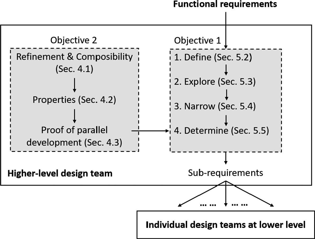
Figure 1 is an overall description of the structure of the proposed approach. After introducing the background information and the preliminaries (Sections 2 and 3), we address Objective 2 first in Section 4 (the left half of Figure 1). It was concluded that to ensure parallel development, the sub-requirements at each level of abstraction must be composable and able to refine the higher-level functional requirements as a whole. This finding will be treated as the constraints of the optimization problem of the requirements decomposition process. After that, we explain the requirements decomposition process based on SBD principles (the right half of Figure 1) in Section 5. Given the functional requirements from the customers or a higher-level design team, a four-step process is applied to define, explore and narrow the possible space of alternatives (Sections 5.2–5.4) and eventually determine the sub-requirements that will be assigned to design teams at the lower levels through an optimization program (Section 5.5). We demonstrate the method with an example of designing a cruise control system based on existing computational tools in Section 6.
The overall structure of the proposed approach.
2. Background
2.1. Set-based design (SBD)
In product development, two main strategies exist for selecting a concept: point-based design (PBD) and SBD. PBD involves choosing a single “best” option early from all possibilities, whereas SBD progressively eliminates infeasible or less attractive alternatives until only one solution remains (Morgan & Liker Reference Morgan and Liker2020). PBD often causes problems because decisions are made too early, based on assumptions or incomplete knowledge, leading to rework, correction loops and risk aversion that can stifle innovation (Majerus Reference Majerus2017).
SBD addresses these issues by maintaining multiple feasible options longer and narrowing them down as knowledge grows. SBD is a structured engineering methodology that emphasizes exploring a wide spectrum of design alternatives rather than fixating on a single solution from the outset. Originating in lean product development, most notably at Toyota (Ward et al. Reference Ward, Liker, Cristiano and Sobek1995), this approach promotes delaying commitment until sufficient knowledge is amassed, enabling more robust trade-offs and reducing costly rework (Verma Reference Verma2023). In SBD, cross-disciplinary teams concurrently maintain multiple feasible design sets, gradually converging through feasibility assessment and intersection of acceptable solution spaces (SEBoK 2025). Unlike traditional point-based or sequential design methods, SBD fosters greater parallelism, improved organizational learning and the capacity to manage uncertainty – especially in early stages with loosely defined requirements or conflicting constraints. Three principles guide SBD: map the design space, integrate by intersection and establish viability before committing (Sobek et al. Reference Sobek, Ward and Liker1999). Mapping the design space involves defining feasibility regions, exploring trade-offs via multiple alternatives and communicating sets (Kerga, Taisch & Terzi Reference Kerga, Taisch and Terzi2013). Integration by intersection ensures that acceptable solutions lie in the overlapping feasible sets of all subsystems, promoting compatibility. Finally, narrowing occurs gradually by refining alternatives, remaining within feasible regions and managing uncertainty at decision gates. Together, these principles make SBD a structured approach for fostering robustness and innovation while avoiding premature commitment. A line of research was conducted recently to examine, by applying computational methods, the benefits and drawbacks of SBD, specifically how SBD interacts with various team and problem structures, using problem coupling and varying timespan to further elucidate the impacts of the process (Rismiller, Cagan & McComb Reference Rismiller, Cagan and McComb2023, Reference Rismiller, Cagan and McComb2024). The results suggest that SBD lowers the need for communication and rework on coupled problems, allowing projects to achieve greater concurrency and break through barriers in the design space to create new designs (Rismiller Reference Rismiller2023).
Recent studies have extended SBD to complex engineering systems, integrating model-based systems engineering (MBSE) to systematically evaluate design options using computational models (Specking et al. Reference Specking, Parnell, Pohl and Buchanan2018b). Advanced applications in automotive, aerospace and construction show that combining SBD with optimization and tradespace exploration enables designers to handle uncertainty, balance conflicting requirements and improve performance early in the development process (Ishikawa Reference Ishikawa2024; Kazuki et al. Reference Kazuki, Nishikawa, Shintani, Kawamura, Suzuki and Tsuchiyama2024; Oyama & Kato Reference Oyama and Kato2024; van Heerden et al. Reference van Heerden, Altelarrea, Riaz, Chen, Guenov and Molina-Cristóbal2024). Recent reviews (Castañeda et al. Reference Castañeda, Herrera, Sánchez and Mejía2023; de Oliveira et al. Reference de Oliveira, Forcellini, Lozano and Barbosa2024) further confirm that, while theoretical development is still evolving, growing research underscores SBD’s growing relevance in enabling lean, flexible and resilient design processes.
2.2. SBD for requirements
2.2.1. Qualitative SBD approaches
It was pointed out that “there is limited SBD research contributing to requirements development (Shallcross et al. Reference Shallcross, Parnell, Pohl and Specking2020)” and that SBD methodologies applied to complex systems are mostly qualitative (Shallcross Reference Shallcross2021). Enhanced function-means modeling (EF-M) is one such method used for function modeling (Müller et al. Reference Müller, Isaksson, Landahl, Raja, Panarotto, Levandowski and Raudberget2019). It has been combined with SBD to manage platform-based product family design (Raudberget, Michaelis & Johannesson Reference Raudberget, Michaelis and Johannesson2014). Functional decomposition and solutions are generated according to EF-M, with mappings from functional requirements (FR) to design solutions (DS) at each level of abstraction (Levandowski, Raudberget & Johannesson Reference Levandowski, Raudberget and Johannesson2014). These mappings align conceptually with our proposed method. A systematic, knowledge-focused framework was proposed to guide early-phase design exploration in a set-based, front-loaded manner (Gamage & Sobek Reference Gamage and Sobek II.2024). This framework offers a step-by-step approach to identifying knowledge requirements in design spaces characterized by multiple objectives and design parameters, ensuring better-informed decisions and fostering innovation in complex product development.
A “wayfaring” model for set-based requirement generation was introduced to discover critical functionalities and create dynamic requirements (Kriesi et al. Reference Kriesi, Blindheim, Bjelland and Steinert2016). This model uses prototyping to guide the design process from initial concept to final product, minimizing tooling and production costs. Model-based requirements and architecture (MBRMA), a novel set-based approach, was developed to filter out weak or costly solutions and assist system engineers in trade-off analysis (Borchani et al. Reference Borchani, Hammadi, Yahia and Choley2019). Although this approach defines a mathematical formalism, it lacks specific guidance on requirement decomposition. A framework based on set-based engineering allows for building reusable and adaptable engineering methods (Vallhagen et al. Reference Vallhagen, Isaksson, Söderberg and Wärmefjord2013). These “virtual methods” help create and validate early phase design requirements, ensuring the introduction of novel technologies without compromising risk and cost. Other frameworks include CONGA (Al-Ashaab et al. Reference Al-Ashaab, Golob, Noriega, Torriani, Alvarez, Beltran, Busachi, Ex-Ignotis, Rigatti and Sharma2013b), DMIV (Ammar et al. Reference Ammar, Hammadi, Choley, Barkallah, Louat and Haddar2017), MBSS (Yvars & Zimmer Reference Yvars and Zimmer2022), RR-LeanPD model (Al-Ashaab et al. Reference Al-Ashaab, Golob, Attia, Khan, Parsons, Andino, Perez, Guzman, Onecha, Kesavamoorthy, Martinez, Shehab, Berkes, Haque, Soril and Sopelana2013a) and a combination of V-model and SBCE (Al-Ashaab et al. Reference Al-Ashaab, Howell, Usowicz, Anta and Gorka2009).
One limitation of these qualitative approaches is the ambiguity surrounding the concrete activities needed for requirements development. This ambiguity makes it challenging for industry practitioners to replicate these methods. A formal method provides precise, repeatable instructions for decomposing functional requirements and assigning them to lower abstraction levels.
2.2.2. Quantitative SBD approaches
Quantitative techniques for design space exploration in SBD often feature hierarchical decomposition. For example, SBD was applied to the design of a downhole module to validate a laboratory-developed method in an actual industry setting (Madhavan et al. Reference Madhavan, Shahan, Seepersad, Hlavinka and Benson2008). The module was decomposed into chassis and bumper subsystems, with design targets assigned based on a downhole assembly impact model. A set-based approach was used for a multilevel design problem of negative stiffness metamaterials, progressing from macro-level to micro-level (Matthews et al. Reference Matthews, Klatt, Morris, Seepersad, Haberman and Shahan2016). Both studies feature hierarchical decomposition but differ from our problem formulation by treating higher-level design spaces as requirements for lower-level design spaces.
Jansson et al. combined SBD with axiomatic design to evaluate multiple design alternatives against functional requirements (Jansson, Schade & Olofsson Reference Jansson, Schade and Olofsson2013). This work mapped higher-level design spaces to lower-level functional requirements but did not detail the derivation process. Shahan & Seepersad proposed a set-based approach to collaborative design, using Bayesian networks to identify compatibilities and conflicts among distributed subsystems (Shahan & Seepersad Reference Shahan and Seepersad2012). However, this approach focused on optimizing top-level objectives rather than decomposing requirements.
Airplane design requirements can be decomposed into design parameters for various components using SBD principles (Kerga et al. Reference Kerga, Rossi, Taisch and Terzi2014). Although educational, this game effectively demonstrated the derivation of lower-level design parameter ranges from higher-level parameters. Panchal et al. presented an interval-based constraint satisfaction method for decentralized, collaborative multifunctional design, systematically reducing interval-based design variables to satisfy requirements (Panchal et al. Reference Panchal, Fernández, Paredis, Allen and Mistree2007). SBD was also used to inform system requirements and evaluate design options for a UAV, demonstrating comprehensive tradespace exploration and valuable insights into requirement development (Parnell et al. Reference Parnell, Specking, Goerger, Cilli and Pohl2019; Specking et al. Reference Specking, Shallcross, Parnell and Pohl2021).
In summary, these approaches treat functional requirements as ranges of performance space variables, unlike our method, which defines requirements as mappings between design and performance spaces. This distinction significantly impacts the requirements decomposition process, with our method focusing on mapping from higher-level function mappings to sub-function mappings.
2.3. Design uncertainty
2.3.1. The SBD approach
SBD is known for its robustness to design uncertainty (Terwiesch, Loch & Meyer Reference Terwiesch, Loch and Meyer2002; Costa & Sobek Reference Costa and Sobek2003; Bogus, Molenaar & Diekmann Reference Bogus, Molenaar and Diekmann2006). The US Naval Sea Systems Command highlighted SBD’s suitability for design problems with conflicting requirements and high uncertainty (Parker et al. Reference Parker, Garner, Arcano and Doerry2017). Trueworthy corroborated this, noting SBD’s flexibility in adjusting to changing requirements (Trueworthy et al. Reference Trueworthy, DuPont, Maurer and Cavagnaro2019). Specifically, flexibility is implemented by initially setting up broad specifications and loose constraints, which can be narrowed down as details emerge (Al Handawi et al. Reference Al Handawi, Brahma, Wynn, Kokkolaras and Isaksson2024).
An approach incorporating Bayesian network classifiers defined “design flexibility” as the subspace size producing satisfactory designs and “performance flexibility” as the feasible performance space size relative to the desired space (Matthews et al. Reference Matthews, Klatt, Seepersad, Haberman and Shahan2014). An SBD methodology was proposed to obtain scalable optimal solutions that satisfy changing requirements through remanufacturing, demonstrated on a structural aeroengine component (Al Handawi et al. Reference Al Handawi, Andersson, Panarotto, Isaksson and Kokkolaras2021). Another line of work combines SBD with platform-based design to preserve design bandwidth, allowing flexibility in different products (Müller, Siiskonen & Malmqvist Reference Müller, Siiskonen and Malmqvist2020). A dynamic platform modeling approach represented production variety streams, reducing the risk of late and costly modifications (Landahl et al. Reference Landahl, Jiao, Madrid, Söderberg and Johannesson2021). Modeling platform concepts in early phases and eliminating undesired regions of the design space were described by (Levandowski et al. Reference Levandowski, Forslund and Johannesson2013; Levandowski et al. Reference Levandowski, Raudberget and Johannesson2014; Levandowski, Müller & Isaksson Reference Levandowski, Müller and Isaksson2016). In addition, McKenney et al. conducted a design experiment showing that delaying decisions using SBD increases adaptability to requirement changes (McKenney, Kemink & Singer Reference McKenney, Kemink and Singer2011). A method called dynamically constrained SBD provided a dynamic map for feasible design space under varying requirements using parametric constraint sensitivity analysis and convex hull techniques (Kizer & Mavris Reference Kizer and Mavris2014). This method identified a robust, feasible design space and a flexible family of solutions. A hybrid agent approach for set-based conceptual ship design found the process robust to intermediate design errors (Parsons & Singer Reference Parsons and Singer1999). Similar work can be found in (Ross Reference Ross2017; (Rapp et al. Reference Rapp, Chinnam, Doerry, Murat and Witus2018).
According to Tackett et al., “excess” is “the quantity of surplus in a system once the necessities are met (Tackett, Mattson & Ferguson Reference Tackett, Mattson and Ferguson2014). Eckert et al. later defined “excess” as “the value over and above any allowances for uncertainties” and “buffer” as “the portion of parameter values that compensates for uncertainties (Eckert et al. Reference Eckert, Isaksson and Earl2019). Current SBD literature lacks an explicit distinction between buffer and excess when addressing uncertainties, reducing specificity in robustness claims.
2.3.2. The margin-based approach
The aforementioned concepts of “buffer” and “excess” stem from a line of research called “design margin” (Eckert et al. Reference Eckert, Isaksson and Earl2019). In the seminal papers (Clarkson, Simons & Eckert Reference Clarkson, Simons and Eckert2004; Claudia Eckert & Zanker Reference Claudia Eckert and Zanker2004), margin was a concept closely related to change and tolerance of changes. In more recent years, we have seen significant movements in this field. El Fassi et al. proposed a graph-theoretical approach – an assumption network – to support the allocation and management of design margins (El Fassi, Guenov & Riaz Reference El Fassi, Guenov and Riaz2020). A design belief network (DBN) was built to help designers determine whether changes can be absorbed without cascading modifications downstream. A method called the margin value method (MVM) was used to analyze an engineering design, localize the excess margin and quantify it considering change absorption potential in relation to design performance deterioration (Brahma & Wynn Reference Brahma and Wynn2020). MVM was then adapted in the context of uncertainty in input specifications so that undesirable effects of margins can be minimized while preventing change propagation (Brahma, Wynn & Isaksson Reference Brahma, Wynn and Isaksson2022). Later, the same team expanded this method to evaluate sets of concepts that are combinatorially generated from an enhanced function-means tree by using surrogate models and novel metrics for evaluating different conceptual alternatives (Al Handawi et al. Reference Al Handawi, Brahma, Wynn, Kokkolaras and Isaksson2024).
“Resilient objects” provide passive protection against disruptive events so that the necessity for complex margins can be reduced at system interfaces (Panarotto & Fernández Reference Panarotto and Fernández2024). It offered a new perspective on how to solve the trade-offs between resilience and complexity when addressing uncertainties in the dynamic landscape of product development. Five robustness indicators were introduced (Juul-Nyholm & Eifler Reference Juul-Nyholm and Eifler2024) based on multi-objective design exploration to tackle two central challenges in engineering design: (1) defining design margins early in the design process, before detailed modeling is possible, and (2) evaluating interdependencies among those margins to prevent cascading effects. As a result, three distinct margin types were identified to help designers assess margin implications even before models are fully defined. A more holistic review of margins throughout the product development process has been explored elsewhere (Brahma et al. Reference Brahma, Ferguson, Eckert and Isaksson2024).
In comparison, although our approach is closely related to margin, our problem is different from those addressed in the current literature on margin. First, the current literature focuses on the margin of design parameters, while our approach aims to introduce margin into the domain and the co-domain of the functions. Furthermore, the concept of hierarchical refinement is relatively rare in the current literature. As recently pointed out, the concept of hierarchy in the margin literature is not well understood (Brahma et al. Reference Brahma, Ferguson, Eckert and Isaksson2024). While Jacobson and Ferguson touched on this concept (Jacobson & Ferguson Reference Jacobson and Ferguson2023), the proposed process was largely informal. In fact, the authors admitted at the end of the paper that better modeling approaches around decomposition are still needed. Finally, although this paper is not originally aimed to contribute to the margin community, we recognize that many concepts utilized in this paper indeed resemble margin (see Section 7.2). We believe the formal framework proposed by this paper can contribute to the vision of a design environment that will eventually connect margin to requirements (Ferguson et al. Reference Ferguson, Brahma, Eckert and Isaksson2024).
3. Preliminaries
In general, functions describe the behavior between inputs and outputs of a system, subsystem, or component. Such a description can be an informal summary or statement, or a formal specification, all the way up to a literal mathematical function prescribing the desired input–output behavior. In the following, we take the latter perspective: the function of a system is a mathematical input–output transformation that describes the overall behavior of a system (Buede Reference Buede1997; Larson & Mattson Reference Larson and Mattson2012).
 $$ \left(x,u,c\right)\overset{f}{\to }y $$
-
• $ f $
represents the transformation between
$ \left(x,u,c\right) $
and
$ y $
.
$ f $
represents the transformation between
$ \left(x,u,c\right) $
and
$ y $
. -
•
$ x $
represents the input variables that the system takes from the environment or other systems. -
•
$ y $
represents the output variables that the system gives in response to the inputs. -
•
$ u $
represents the uncertain design parameters that are out of the designer’s control, such as the weather for an airplane. We call them the uncontrollable parameters. -
•
$ c $
represents the uncertain design parameters that are under the designer’s control, such as the weight of an airplane. We call them the controllable parameters.


Note that $ x,y,u $
and
$ x,y,u $
and $ c $
are all column vectors of
$ c $
are all column vectors of $ f $
, as a function likely has multiple input variables, output variables, controllable parameters and uncontrollable parameters.
$ f $
, as a function likely has multiple input variables, output variables, controllable parameters and uncontrollable parameters.
3.1. Notation
We introduce the notation used throughout this paper.
-
•
$ f $
and
$ {f}_i $
:
$ f $
is the higher-level function to be decomposed into multiple sub-functions
$ {f}_i $
, where
$ i=1,2,\dots, m $
. -
•
$ a(i) $
: As mentioned above,
$ x,y,u $
and
$ c $
are the four column vectors of
$ f $
. Similarly, the four column vectors of the sub-function
$ {f}_i $
are denoted as
$ x(i),y(i),u(i) $
and
$ c(i) $
. Abstractly, we denote these column vectors with a unified expression
$ a(i) $
, where
$ a(i)={\left({a}_1(i),{a}_2(i),\dots, {a}_n(i)\right)}^{\top } $
. -
•
$ {a}_j(i) $
, as the
$ {j}^{th} $
element of
$ a(i) $
, represents one individual input/output variable or controllable/uncontrollable parameter of sub-function
$ {f}_i $
(where
$ j=1,2\dots, n $
). -
•
$ {R}_{a_j(i)} $
is the range of
$ {a}_j(i) $
, that is,
$ {a}_j(i)\in {R}_{a_j(i)} $
. -
•
$ \left\{a(i)\right\} $
is a set representation of
$ a(i) $
, that is,
$ \left\{a(i)\right\}=\left\{{a}_1(i),{a}_2(i),\dots, {a}_n(i)\right\} $
. -
•
$ {R}_{a(i)}={\left({R}_{a_1(i)},{R}_{a_2(i)},\dots, {R}_{a_n(i)}\right)}^{\top } $
is a column vector of the ranges of
$ a(i) $
. -
•
$ \left\{{R}_{a(i)}\right\} $
is a set representation of
$ {R}_{a(i)} $
, that is,
$ \left\{{R}_{a(i)}\right\}=\left\{{R}_{a_1(i)},{R}_{a_2(i)},\dots, {R}_{a_n(i)}\right\} $
.
















We now define the following set operations, where $ a $
and
$ a $
and $ b $
are two column vectors.
$ b $
are two column vectors.
-
•
$ \left\{a\right\}\bigsqcup \left\{b\right\} $
returns the union of the identifiers (instead of the values) of all the elements in
$ \left\{a\right\} $
and
$ \left\{b\right\} $
. The identical variable between
$ \left\{a\right\} $
and
$ \left\{b\right\} $
is merged into one element. By “identical,” we mean the elements that have the same physical meaning, the same data source and hence the same value at all times. -
•
$ \left\{a\right\}\sqcap \left\{b\right\} $
returns the identifier of the identical variable(s) between
$ \left\{a\right\} $
and
$ \left\{b\right\} $
. -
•
$ \left\{a\right\}\sqsubseteq \left\{b\right\} $
returns true if the identifiers (instead of the values) of all the variables in
$ \left\{a\right\} $
are included in
$ \left\{b\right\} $
. -
•
$ \left\{{R}_a\right\}\Cup \left\{{R}_b\right\} $
returns the set of the ranges of
$ \left\{a\right\}\bigsqcup \left\{b\right\} $
. Because the identical elements between
$ \left\{a\right\} $
and
$ \left\{b\right\} $
are subject to the ranges in both
$ \left\{{R}_a\right\} $
and
$ \left\{{R}_b\right\} $
, the resulting ranges for the identical elements are the intersections (
$ \cap $
) of the respective ranges in
$ \left\{{R}_a\right\} $
and
$ \left\{{R}_b\right\} $
. -
•
$ {a}_j\mid \left\{{R}_b\right\} $
identifies the element in
$ \left\{b\right\} $
that is identical to
$ {a}_j $
and returns its range in
$ \left\{{R}_b\right\} $
. -
•
$ \mathcal{T}\mathcal{R}(\{{R}_a\}) $
transforms the set
$ \left\{{R}_a\right\} $
into the column vector
$ {R}_a $
,that is,
$ \mathcal{T}\mathcal{R}(\{{R}_a\})={R}_a $
.



3.2. Functional requirements
Mathematically, a system function, as defined in Eq. (1), must satisfy Eq. (2), where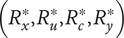 $ \left({R}_x^{\ast },{R}_u^{\ast },{R}_c^{\ast },{R}_y^{\ast}\right) $
constitute the functional requirements of the system.
$ \left({R}_x^{\ast },{R}_u^{\ast },{R}_c^{\ast },{R}_y^{\ast}\right) $
constitute the functional requirements of the system.
 $$ \forall x\in {R}_x^{\ast },\forall u\in {R}_u^{\ast },\exists c\in {R}_c^{\ast }:\left(x,u,c\right)\overset{f}{\to }y\in {R}_y^{\ast } $$
-
•
$ \forall {R}_x^{\ast } $
implies the system must be able to process all the values from the input set. -
•
$ \forall {R}_u^{\ast } $
is because
$ u $
is out of the designer’s control. The system must be able to process all possible
$ u $
. -
•
$ \exists {R}_c^{\ast } $
is because
$ c $
is under the designer’s control. The designer only needs to find one
$ c $
within
$ {R}_c^{\ast } $
to satisfy the functional requirements. -
•
$ {R}_y^{\ast } $
is the co-domain of
$ f $
. All possible output values must be bounded within
$ {R}_y^{\ast } $
.


However, not any random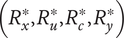 $ \left({R}_x^{\ast },{R}_u^{\ast },{R}_c^{\ast },{R}_y^{\ast}\right) $
can be the requirements of
$ \left({R}_x^{\ast },{R}_u^{\ast },{R}_c^{\ast },{R}_y^{\ast}\right) $
can be the requirements of $ f $
.
$ f $
. $ \left({R}_x^{\ast },{R}_u^{\ast },{R}_c^{\ast}\right) $
and
$ \left({R}_x^{\ast },{R}_u^{\ast },{R}_c^{\ast}\right) $
and $ {R}_y^{\ast } $
must satisfy Eq. (3), which implies that the functional requirements of a system are actually a constrained mapping between
$ {R}_y^{\ast } $
must satisfy Eq. (3), which implies that the functional requirements of a system are actually a constrained mapping between $ \left({R}_x^{\ast },{R}_u^{\ast },{R}_c^{\ast}\right) $
and
$ \left({R}_x^{\ast },{R}_u^{\ast },{R}_c^{\ast}\right) $
and $ {R}_y^{\ast } $
.
$ {R}_y^{\ast } $
.
 $$ \left({R}_x^{\ast },{R}_c^{\ast },{R}_u^{\ast}\right)\to {R}_y^{\ast}\;\mathrm{s}.\mathrm{t}.\mathrm{Eq}.(2) $$
Similarly, the requirements of $ {f}_i $
can be represented as:
$ {f}_i $
can be represented as:
 $$ \left({R}_{x(i)}^{\ast },{R}_{c(i)}^{\ast },{R}_{u(i)}^{\ast}\right)\to {R}_{y(i)}^{\ast}\;\mathrm{s}.\mathrm{t}.\mathrm{Eq}.(2) $$
Therefore, the functional requirements decomposition problem is to decompose the top-level requirements in Eq. (3) into a set of sub-requirements in Eq. (4) at the lower level, repeat the same process independently at each level of abstraction and eventually lead to a system that satisfies the top-level requirements in Eq. (3).
4. Parallel development
We explain in this that refinement and composability are the two constraints to ensure parallel development (i.e., Objective 2).
4.1. Refinement and composability
Refinement and composability play an important role in producing traceable requirements.
4.1.1. Refinement
Refinement defines a relationship between two sets of functional requirements (FR). $ F{R}^{\prime } $
refining
$ F{R}^{\prime } $
refining $ FR $
implies the reduction of the uncertainties from
$ FR $
implies the reduction of the uncertainties from $ FR $
to
$ FR $
to $ F{R}^{\prime } $
, which can always be reflected in the mapping between the input and output variables. As shown in Figure 2(a),
$ F{R}^{\prime } $
, which can always be reflected in the mapping between the input and output variables. As shown in Figure 2(a), $ F{R}^{\prime } $
refines
$ F{R}^{\prime } $
refines $ FR $
if the relationship in Eq. (5) is satisfied, where the meanings of
$ FR $
if the relationship in Eq. (5) is satisfied, where the meanings of $ {x}_i\mid \left\{{R}_{x^{\prime}}^{\ast}\right\} $
and
$ {x}_i\mid \left\{{R}_{x^{\prime}}^{\ast}\right\} $
and $ {y}_i\mid \left\{{R}_{y^{\prime}}^{\ast}\right\} $
are defined in Section 3.1.
$ {y}_i\mid \left\{{R}_{y^{\prime}}^{\ast}\right\} $
are defined in Section 3.1.
 $$ \left\{\begin{array}{c}\left\{x\right\}\sqsubseteq \left\{{x}^{\prime}\right\}\wedge \forall {x}_i\in \left\{x\right\}:{R}_{x_i}^{\ast}\subseteq {x}_i\mid \left\{{R}_{x^{\prime}}^{\ast}\right\}\\ {}\left\{y\right\}\sqsubseteq \left\{{y}^{\prime}\right\}\wedge \forall {y}_i\in \left\{y\right\}:{y}_i\mid \left\{{R}_{y^{\prime}}^{\ast}\right\}\subseteq {R}_{y_i}^{\ast}\end{array}\right. $$
Graphical illustration of refinement. The green circles are the ranges defined in $ FR $
, and the brown circles are the ranges defined in
$ FR $
, and the brown circles are the ranges defined in $ F{R}^{\prime } $
.
$ F{R}^{\prime } $
.
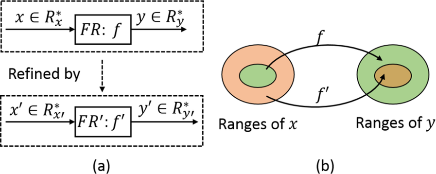
Intuitively, Eq. (5) means (1) $ F{R}^{\prime } $
defines all the input/output variables of
$ F{R}^{\prime } $
defines all the input/output variables of $ FR $
, and (2)
$ FR $
, and (2) $ F{R}^{\prime } $
allows the system to take a larger range of
$ F{R}^{\prime } $
allows the system to take a larger range of $ x $
but will generate a smaller range of
$ x $
but will generate a smaller range of $ y $
than
$ y $
than $ FR $
.
$ FR $
.
Note that a system satisfying the functional requirements is a special case of refinement. As implied by Eq. (2), the system can take all the values in $ {R}_x^{\ast } $
and provide the output values that are bounded within
$ {R}_x^{\ast } $
and provide the output values that are bounded within $ {R}_y^{\ast } $
, which satisfies the relationship of refinement in Eq. (5).
$ {R}_y^{\ast } $
, which satisfies the relationship of refinement in Eq. (5).
4.1.2. Composability
Composability defines the interface between functional requirements. Therefore, only the input and output variables are concerned. Two sets of functional requirements (denoted as $ {FR}_j $
and
$ {FR}_j $
and $ {FR}_k $
in Figure 3(a)) are composable if the relationship in Eq. (6) below is satisfied.
$ {FR}_k $
in Figure 3(a)) are composable if the relationship in Eq. (6) below is satisfied.
 $$ \left\{\begin{array}{l}\left\{z\right\}=\left\{y(j)\right\}\sqcap \left\{x(k)\right\}\ne 0\\ {}\forall {z}_i\in \left\{z\right\}:{z}_i\mid \left\{{R}_{y(j)}^{\ast}\right\}\subseteq {z}_i\mid \left\{{R}_{x(k)}^{\ast}\right\}\end{array}\right. $$
Graphical illustration of composability. The green circles are the ranges defined in $ {FR}_j $
, and the brown circles are the ranges defined in
$ {FR}_j $
, and the brown circles are the ranges defined in $ {FR}_k $
.
$ {FR}_k $
.

Intuitively, composability means two things: (1) the output of $ {FR}_j $
and the input of
$ {FR}_j $
and the input of $ {FR}_k $
share at least one common variable (denoted as
$ {FR}_k $
share at least one common variable (denoted as $ \left\{z\right\} $
), and (2)
$ \left\{z\right\} $
), and (2) $ {FR}_k $
can take in more values of
$ {FR}_k $
can take in more values of $ z $
than
$ z $
than $ {FR}_j $
can output (Figure 3(b)).
$ {FR}_j $
can output (Figure 3(b)).
4.2. Properties of refinement and composability
Based on the definitions above, we have the following properties.
Property 1. If $ F{R}^{\prime } $
refines
$ F{R}^{\prime } $
refines $ FR $
, and
$ FR $
, and $ F{R^{\prime}}^{\prime } $
refines
$ F{R^{\prime}}^{\prime } $
refines $ F{R}^{\prime } $
, then
$ F{R}^{\prime } $
, then $ F{R^{\prime}}^{\prime } $
refines
$ F{R^{\prime}}^{\prime } $
refines $ FR $
.
$ FR $
.
Property 2. If a set of functional requirements $ \left\{{FR}_1,{FR}_2,\dots, {FR}_n\right\} $
are composable, then their refinements
$ \left\{{FR}_1,{FR}_2,\dots, {FR}_n\right\} $
are composable, then their refinements $ \left\{F{R}_1^{\prime },F{R}_2^{\prime },\dots, F{R}_n^{\prime}\right\} $
are also composable.
$ \left\{F{R}_1^{\prime },F{R}_2^{\prime },\dots, F{R}_n^{\prime}\right\} $
are also composable.
Property 3. Consider a set of composable functional requirements $ \left\{{FR}_1,{FR}_2,\dots, {FR}_n\right\} $
. If
$ \left\{{FR}_1,{FR}_2,\dots, {FR}_n\right\} $
. If $ F{R}_i^{\prime } $
refines
$ F{R}_i^{\prime } $
refines $ {FR}_i $
(i = 1,2,n), then the composite of
$ {FR}_i $
(i = 1,2,n), then the composite of $ \left\{F{R}_1^{\prime },F{R}_2^{\prime },\dots, F{R}_n^{\prime}\right\} $
refines the composite of
$ \left\{F{R}_1^{\prime },F{R}_2^{\prime },\dots, F{R}_n^{\prime}\right\} $
refines the composite of $ \left\{{FR}_1,{FR}_2,\dots, {FR}_n\right\} $
.
$ \left\{{FR}_1,{FR}_2,\dots, {FR}_n\right\} $
.
Because a system satisfying the functional requirements is a special case of refinement, Properties 4, 5 and 6 can be derived similarly to Properties 1, 2 and 3.
Property 4. If $ F{R}^{\prime } $
refines
$ F{R}^{\prime } $
refines $ FR $
, and a system
$ FR $
, and a system $ S $
satisfies
$ S $
satisfies $ F{R}^{\prime } $
, then
$ F{R}^{\prime } $
, then $ S $
satisfies
$ S $
satisfies $ FR $
.
$ FR $
.
Property 5. If a set of functional requirements $ \left\{{FR}_1,{FR}_2,\dots, {FR}_n\right\} $
are composable, and a set of systems
$ \left\{{FR}_1,{FR}_2,\dots, {FR}_n\right\} $
are composable, and a set of systems $ \left\{{S}_1,{S}_2,\dots, {S}_n\right\} $
satisfy the functional requirements, respectively, then
$ \left\{{S}_1,{S}_2,\dots, {S}_n\right\} $
satisfy the functional requirements, respectively, then $ \left\{{S}_1,{S}_2,\dots, {S}_n\right\} $
are also composable.
$ \left\{{S}_1,{S}_2,\dots, {S}_n\right\} $
are also composable.
Property 6. Consider a set of composable functional requirements $ \left\{{FR}_1,{FR}_2,\dots, {FR}_n\right\} $
and their composite
$ \left\{{FR}_1,{FR}_2,\dots, {FR}_n\right\} $
and their composite $ FR $
. If
$ FR $
. If $ {S}_i $
satisfies
$ {S}_i $
satisfies $ {FR}_i $
(i = 1,2,…,n), then the composite of
$ {FR}_i $
(i = 1,2,…,n), then the composite of $ \left\{{S}_1,{S}_2,\dots, {S}_n\right\} $
satisfies the composite of
$ \left\{{S}_1,{S}_2,\dots, {S}_n\right\} $
satisfies the composite of $ \left\{{FR}_1,{FR}_2,\dots, {FR}_n\right\} $
.
$ \left\{{FR}_1,{FR}_2,\dots, {FR}_n\right\} $
.
4.3. Ensuring parallel development
In this subsection, we illustrate, with a simple system (Figure 4), the hierarchical functional requirements decomposition process and prove the conditions under which the decomposed requirements ensure the top-level functional requirements are satisfied.
A two-level example system to describe the hierarchical functional requirements decomposition process.
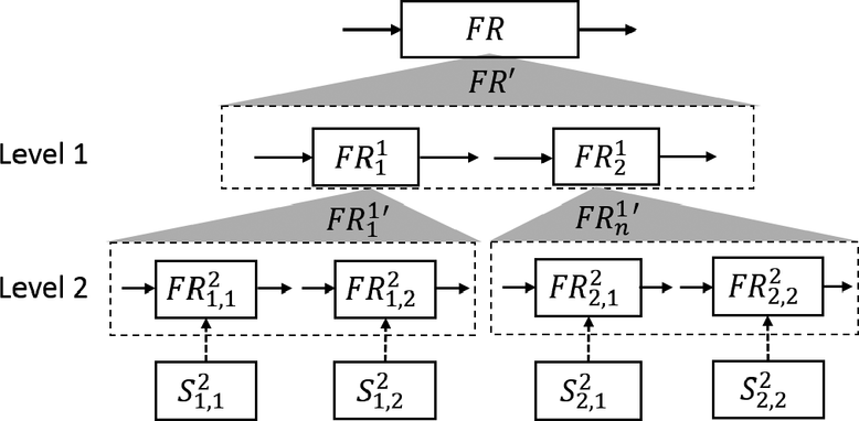
First, the given top-level functional requirements $ FR $
are decomposed into
$ FR $
are decomposed into $ \left\{{FR}_1^1,{FR}_2^1\right\} $
and assigns them to the Level-1 suppliers. The Level-1 suppliers then independently decompose
$ \left\{{FR}_1^1,{FR}_2^1\right\} $
and assigns them to the Level-1 suppliers. The Level-1 suppliers then independently decompose $ {FR}_1^1 $
and
$ {FR}_1^1 $
and $ {FR}_2^1 $
into
$ {FR}_2^1 $
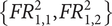
into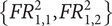 $ \left\{{FR}_{1,1}^2,{FR}_{1,2}^2\right\} $
and
$ \left\{{FR}_{1,1}^2,{FR}_{1,2}^2\right\} $
and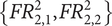 $ \left\{{FR}_{2,1}^2,{FR}_{2,2}^2\right\} $
, respectively, and assign these to Level-2 suppliers. The Level-2 suppliers implement the functional requirements independently in individual systems
$ \left\{{FR}_{2,1}^2,{FR}_{2,2}^2\right\} $
, respectively, and assign these to Level-2 suppliers. The Level-2 suppliers implement the functional requirements independently in individual systems $ {S}_{1,1}^2,{S}_{1,2}^2,{S}_{2,1}^2 $
, and
$ {S}_{1,1}^2,{S}_{1,2}^2,{S}_{2,1}^2 $
, and $ {S}_{2,2}^2 $
that satisfy the respective functional requirements.
$ {S}_{2,2}^2 $
that satisfy the respective functional requirements.
We now prove that if at each level of abstraction, (1) the sub-requirements are composable, and (2) when composed together, the sub-requirements refine the higher-level functional requirements, then $ {S}_{1,1}^2,{S}_{1,2}^2,{S}_{2,1}^2 $
, and
$ {S}_{1,1}^2,{S}_{1,2}^2,{S}_{2,1}^2 $
, and $ {S}_{2,2}^2 $
are composable and together satisfy
$ {S}_{2,2}^2 $
are composable and together satisfy $ FR $
.
$ FR $
.
Proof:
-
1. By definition,
$ \left\{{FR}_1^1,{FR}_2^1\right\} $
are composable and refine
$ FR $
;
$ \left\{{FR}_{1,1}^2,{FR}_{1,2}^2\right\} $
are composable and refine
$ {FR}_1^1 $
;
$ \left\{{FR}_{2,1}^2,{FR}_{2,2}^2\right\} $
are composable and refine
$ {FR}_2^1 $
;
$ {S}_{1,1}^2,{S}_{1,2}^2,{S}_{2,1}^2 $
and
$ {S}_{2,2}^2 $
satisfy
$ {FR}_{1,1}^2,{FR}_{1,2}^2,{FR}_{2,1}^2 $
and
$ {FR}_{2,2}^2 $
, respectively. -
2. According to Property 2,
$ \left\{{FR}_{1,1}^2,{FR}_{1,2}^2,{FR}_{2,1}^2,{FR}_{2,2}^2\right\} $
are composable. Then, the composite of
$ \left\{{FR}_{1,1}^2,{FR}_{1,2}^2,{FR}_{2,1}^2,{FR}_{2,2}^2\right\} $
refines the composite of
$ \left\{{FR}_1^1,{FR}_2^1\right\} $
according to Property 3. Because
$ \left\{{FR}_1^1,{FR}_2^1\right\} $
refine
$ FR $
, the composite of the form
$ \left\{{FR}_{1,1}^2,{FR}_{1,2}^2,{FR}_{2,1}^2,{FR}_{2,2}^2\right\} $
refines
$ FR $
according to Property 1. -
3. Since
$ \left\{{FR}_{1,1}^2,{FR}_{1,2}^2,{FR}_{2,1}^2,{FR}_{2,2}^2\right\} $
are composable, and
$ {S}_{1,1}^2,{S}_{1,2}^2,{S}_{2,1}^2 $
$ {S}_{2,2}^2 $
satisfy
$ {FR}_{1,1}^2,{FR}_{1,2}^2,{FR}_{2,1}^2 $
and
$ {FR}_{2,2}^2 $
, respectively, then
$ \left\{{S}_{1,1}^2,{S}_{1,2}^2,{S}_{2,1}^2,{S}_{2,2}^2\right\} $
are composable according to Property 5. The composite of
$ \left\{{S}_{1,1}^2,{S}_{1,2}^2,{S}_{2,1}^2,{S}_{2,2}^2\right\} $
satisfies the composite of
$ \left\{{FR}_{1,1}^2,{FR}_{1,2}^2,{FR}_{2,1}^2,{FR}_{2,2}^2\right\} $
according to Property 6. We have established that the composite of
$ \left\{{FR}_{1,1}^2,{FR}_{1,2}^2,{FR}_{2,1}^2,{FR}_{2,2}^2\right\} $
refines
$ FR $
. Then, according to Property 4, the composite of
$ \left\{{S}_{1,1}^2,{S}_{1,2}^2,{S}_{2,1}^2,{S}_{2,2}^2\right\} $
satisfies
$ FR $
. In other words, the resulting system satisfies the top-level functional requirements.



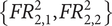




















Therefore, for design teams at different levels of abstraction to work in parallel and obtain a system that satisfies the top-level functional requirements, the sub-requirements at each level of abstraction must be composable and refine the higher-level functional requirements as a whole.
5. Set-based requirements decomposition
In this section, we explain the set-based requirements decomposition process to tackle ambiguity and uncertainty in requirements decomposition (i.e., Objective 1).
5.1. An overall description
Given the higher-level functional requirements, the decomposition process involves the following steps:
-
1. Define and analyze the functional architecture (Section 5.2). A set of functional architecture (comprising a set of connected sub-functions) for the system-under-design is defined to refine the higher-level functional requirements, based on which the design space and the performance space are derived.
-
2. Explore the sub-functions for initial feasible spaces (Section 5.3). A set of initial feasible spaces of the sub-functions is characterized individually by exploring the different feasible implementations for the corresponding sub-functions.
-
3. Narrow the initial feasible spaces(Section 5.4). The feasible design space and the feasible performance space of the system-under-design are narrowed gradually by taking “intersections” based on the initial feasible spaces of the sub-functions.
-
4. Determine the sub-requirements (Section 5.5). The functional requirements of each sub-function are defined based on the narrowed feasible design space and performance space so that all the sub-requirements are composable, and when composed together, they can refine the higher-level functional requirements.
After that, the team for each sub-function will improve the level of detail by independently decomposing the sub-functions into the lower levels iteratively until a final solution can be chosen.
5.2. Define and analyze the functional architecture
A functional architecture is composed of a set of connected sub-functions (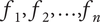 $ {f}_1,{f}_2,\dots, {f}_n $
) and represents a set of potential design solutions for the higher-level requirements. In SBD, there can be multiple alternative functional architectures. However, from the perspective of formal reasoning, the process to derive the sub-requirements for any functional architecture is the same. Therefore, we assume in this paper that only one functional architecture is defined in this step. In addition, the identification of the functional architecture relies on the designer’s understanding of the desired system (Benveniste et al. Reference Benveniste, Caillaud, Nickovic, Passerone, Raclet, Reinkemeier, Sangiovanni-Vincentelli, Damm, Henzinger and Larsen2015). The techniques to identify functional architecture are out of the scope of this paper, but can be found elsewhere (Komoto & Tomiyama Reference Komoto and Tomiyama2011; Penzenstadler Reference Penzenstadler2011; She et al. Reference She, Belanger, Bartels and Reeling2022).
$ {f}_1,{f}_2,\dots, {f}_n $
) and represents a set of potential design solutions for the higher-level requirements. In SBD, there can be multiple alternative functional architectures. However, from the perspective of formal reasoning, the process to derive the sub-requirements for any functional architecture is the same. Therefore, we assume in this paper that only one functional architecture is defined in this step. In addition, the identification of the functional architecture relies on the designer’s understanding of the desired system (Benveniste et al. Reference Benveniste, Caillaud, Nickovic, Passerone, Raclet, Reinkemeier, Sangiovanni-Vincentelli, Damm, Henzinger and Larsen2015). The techniques to identify functional architecture are out of the scope of this paper, but can be found elsewhere (Komoto & Tomiyama Reference Komoto and Tomiyama2011; Penzenstadler Reference Penzenstadler2011; She et al. Reference She, Belanger, Bartels and Reeling2022).
Given a functional architecture, we extract the following two pieces of information: (1) which variable/parameter is shared with which function/sub-functions, and (2) the constitution of the design space and the performance space. These will be used to narrow the feasible spaces later.
First, we aggregate $ x(i),y(i),c(i) $
, and
$ x(i),y(i),c(i) $
, and $ u(i) $
of the sub-functions into
$ u(i) $
of the sub-functions into $ \left\{{x}^{\prime}\right\},\left\{{y}^{\prime}\right\},\left\{{c}^{\prime}\right\} $
, and
$ \left\{{x}^{\prime}\right\},\left\{{y}^{\prime}\right\},\left\{{c}^{\prime}\right\} $
, and $ \left\{{u}^{\prime}\right\} $
without considering the functional architecture. As defined in Section 3.1, the
$ \left\{{u}^{\prime}\right\} $
without considering the functional architecture. As defined in Section 3.1, the $ \bigsqcup $
operation merges the identical variables/parameters in multiple sub-functions into one variable/parameter in the new set.
$ \bigsqcup $
operation merges the identical variables/parameters in multiple sub-functions into one variable/parameter in the new set.
 $$ \left\{\begin{array}{c}\left\{{x}^{\prime}\right\}=\left\{x(1)\right\}\bigsqcup \left\{x(2)\right\}\bigsqcup \dots \bigsqcup \left\{x(n)\right\}\\ {}\left\{{y}^{\prime}\right\}=\left\{y(1)\right\}\bigsqcup \left\{y(2)\right\}\bigsqcup \dots \bigsqcup \left\{y(n)\right\}\\ {}\left\{{c}^{\prime}\right\}=\left\{c(1)\right\}\bigsqcup \left\{c(2)\right\}\bigsqcup \dots \bigsqcup \left\{c(n)\right\}\\ {}\left\{{u}^{\prime}\right\}=\left\{u(1)\right\}\bigsqcup \left\{u(2)\right\}\bigsqcup \dots \bigsqcup \left\{u(n)\right\}\end{array}\right. $$
Second, for the system to implement the higher-level functional requirements, all the elements defined in the higher-level function $ f $
(i.e.,
$ f $
(i.e.,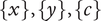 $ \left\{x\right\},\left\{y\right\},\left\{c\right\} $
, and
$ \left\{x\right\},\left\{y\right\},\left\{c\right\} $
, and $ \left\{u\right\} $
) must also be defined in the functional architecture, i.e.,
$ \left\{u\right\} $
) must also be defined in the functional architecture, i.e.,
 $$ \left\{x\right\}\sqsubseteq \left\{{x}^{\prime}\right\}\wedge \left\{c\right\}\sqsubseteq \left\{{c}^{\prime}\right\}\wedge \left\{u\right\}\sqsubseteq \left\{{u}^{\prime}\right\}\wedge \left\{y\right\}\sqsubseteq \left\{{y}^{\prime}\right\} $$
Third, we examine where the variables and the parameters are defined. The elements of $ \left\{{c}^{\prime}\right\} $
and
$ \left\{{c}^{\prime}\right\} $
and $ \left\{{u}^{\prime}\right\} $
may or may not be defined in
$ \left\{{u}^{\prime}\right\} $
may or may not be defined in $ \left\{c\right\} $
and
$ \left\{c\right\} $
and $ \left\{u\right\} $
. We define the elements of
$ \left\{u\right\} $
. We define the elements of $ \left\{{c}^{\prime}\right\} $
and
$ \left\{{c}^{\prime}\right\} $
and $ \left\{{u}^{\prime}\right\} $
that are not defined in
$ \left\{{u}^{\prime}\right\} $
that are not defined in $ \left\{c\right\} $
and
$ \left\{c\right\} $
and $ \left\{u\right\} $
as
$ \left\{u\right\} $
as $ \left\{\tilde{c}\right\} $
and
$ \left\{\tilde{c}\right\} $
and $ \left\{\tilde{u}\right\} $
, and thus have
$ \left\{\tilde{u}\right\} $
, and thus have

For $ \left\{{x}^{\prime}\right\} $
and
$ \left\{{x}^{\prime}\right\} $
and $ \left\{{y}^{\prime}\right\} $
, we use Figure 5 to reason about where the elements can possibly be defined.
$ \left\{{y}^{\prime}\right\} $
, we use Figure 5 to reason about where the elements can possibly be defined. $ \left\{{x}^{\prime}\right\} $
and
$ \left\{{x}^{\prime}\right\} $
and $ \left\{{y}^{\prime}\right\} $
are the two outer ovals that include
$ \left\{{y}^{\prime}\right\} $
are the two outer ovals that include $ \left\{x\right\} $
and
$ \left\{x\right\} $
and $ \left\{y\right\} $
.
$ \left\{y\right\} $
. $ \left\{{x}^{\prime}\right\} $
and
$ \left\{{x}^{\prime}\right\} $
and $ \left\{{y}^{\prime}\right\} $
can be divided into six groups to reason about the design space and the performance space. The ranges of each group will be calculated differently in Section 5.4.
$ \left\{{y}^{\prime}\right\} $
can be divided into six groups to reason about the design space and the performance space. The ranges of each group will be calculated differently in Section 5.4.
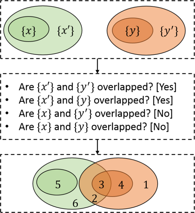
As shown in the middle of Figure 5, there are four possible different ways of where $ \left\{{x}^{\prime}\right\} $
and
$ \left\{{x}^{\prime}\right\} $
and $ \left\{{y}^{\prime}\right\} $
can be defined.
$ \left\{{y}^{\prime}\right\} $
can be defined. $ \left\{{x}^{\prime}\right\} $
and
$ \left\{{x}^{\prime}\right\} $
and $ \left\{{y}^{\prime}\right\} $
overlap because the sub-functions are connected, i.e., one’s input is another’s output;
$ \left\{{y}^{\prime}\right\} $
overlap because the sub-functions are connected, i.e., one’s input is another’s output; $ \left\{{x}^{\prime}\right\} $
and
$ \left\{{x}^{\prime}\right\} $
and $ \left\{y\right\} $
overlap if there are feedback loops that feed some elements of
$ \left\{y\right\} $
overlap if there are feedback loops that feed some elements of $ \left\{y\right\} $
into the sub-functions.
$ \left\{y\right\} $
into the sub-functions. $ \left\{x\right\} $
does not overlap with
$ \left\{x\right\} $
does not overlap with $ \left\{{y}^{\prime}\right\} $
or
$ \left\{{y}^{\prime}\right\} $
or $ \left\{y\right\} $
because
$ \left\{y\right\} $
because $ \left\{x\right\} $
are the input variables of the higher-level functional requirements, hence can only come from the external environment rather than being controlled by the system itself. As a result, we identify six different areas (the bottom of Figure 5) depending on the overlapping between
$ \left\{x\right\} $
are the input variables of the higher-level functional requirements, hence can only come from the external environment rather than being controlled by the system itself. As a result, we identify six different areas (the bottom of Figure 5) depending on the overlapping between $ \left\{{x}^{\prime}\right\},\left\{{y}^{\prime}\right\},\left\{x\right\} $
, and
$ \left\{{x}^{\prime}\right\},\left\{{y}^{\prime}\right\},\left\{x\right\} $
, and $ \left\{y\right\} $
.
$ \left\{y\right\} $
.
The variables in Areas 1, 2, 3 and 4 are, therefore, denoted as $ \left\{{y^{\prime}}^{(1)}\right\},\left\{{y^{\prime}}^{(2)}\right\},\left\{{y^{\prime}}^{(3)}\right\} $
, and
$ \left\{{y^{\prime}}^{(1)}\right\},\left\{{y^{\prime}}^{(2)}\right\},\left\{{y^{\prime}}^{(3)}\right\} $
, and $ \left\{{y^{\prime}}^{(4)}\right\} $
in
$ \left\{{y^{\prime}}^{(4)}\right\} $
in
 $$ \left\{\begin{array}{l}\left\{{y^{\prime}}^{(1)}\right\}=\left\{{y}^{\prime}\right\}\sqcap \neg \left\{y\right\}\sqcap \neg \left\{{x}^{\prime}\right\}\\ {}\left\{{y^{\prime}}^{(2)}\right\}=\left\{{y}^{\prime}\right\}\sqcap \left\{{x}^{\prime}\right\}\sqcap \neg \left\{y\right\}\\ {}\left\{{y^{\prime}}^{(3)}\right\}=\left\{y\right\}\sqcap \left\{{x}^{\prime}\right\}\\ {}\left\{{y^{\prime}}^{(4)}\right\}=\left\{y\right\}\sqcap \neg \left\{{x}^{\prime}\right\}\end{array}\right. $$
Area 5 is $ \left\{x\right\} $
. Area 6, denoted as
$ \left\{x\right\} $
. Area 6, denoted as $ \left\{\tilde{x}\right\} $
, can then be represented as
$ \left\{\tilde{x}\right\} $
, can then be represented as
 $$ \left\{\tilde{x}\right\}=\left\{{x}^{\prime}\right\}\sqcap \neg \left\{{y}^{\prime}\right\}\sqcap \neg \left\{x\right\} $$
Therefore, we can classify all the elements of a functional architecture into the exclusive groups below based on where the elements are defined.
-
•
$ \left\{x\right\} $
is defined in
$ \left\{x\right\} $
and
$ \left\{{x}^{\prime}\right\} $
;
$ \left\{\tilde{x}\right\} $
is only defined within
$ \left\{{x}^{\prime}\right\} $
. -
•
$ \left\{c\right\} $
is defined in
$ \left\{c\right\} $
and
$ \left\{{c}^{\prime}\right\} $
;
$ \left\{\tilde{c}\right\} $
is only defined within
$ \left\{{c}^{\prime}\right\} $
. -
•
$ \left\{u\right\} $
is defined in
$ \left\{u\right\} $
and
$ \left\{{u}^{\prime}\right\} $
;
$ \left\{\tilde{u}\right\} $
is only defined within
$ \left\{{u}^{\prime}\right\} $
. -
•
$ \left\{{y^{\prime}}^{(1)}\right\} $
is only defined in
$ \left\{{y}^{\prime}\right\} $
;
$ \left\{{y^{\prime}}^{(2)}\right\} $
is defined in
$ \left\{{x}^{\prime}\right\} $
and
$ \left\{{y}^{\prime}\right\} $
;
$ \left\{{y^{\prime}}^{(3)}\right\} $
is defined in
$ \left\{{x}^{\prime}\right\},\left\{y\right\} $
, and
$ \left\{{y}^{\prime}\right\} $
;
$ \left\{{y^{\prime}}^{(4)}\right\} $
is defined in
$ \left\{y\right\} $
and
$ \left\{{y}^{\prime}\right\} $
.


Finally, because the design space is the set of the independent variables/parameters of a system, and the performance space is the set of the dependent variables (Wood & Antonsson Reference Wood and Antonsson1989; Nahm & Ishikawa Reference Nahm and Ishikawa2006), the design space and the performance space of the system can be summarized in Eq. (12).
 $$ \left\{\begin{array}{l}\mathrm{Design}\ \mathrm{space}:\left\{x\right\}\bigsqcup \left\{\tilde{x}\right\}\bigsqcup \left\{c\right\}\bigsqcup \left\{\tilde{c}\right\}\bigsqcup \left\{u\right\}\bigsqcup \left\{\tilde{u}\right\}\\ {}\mathrm{Performance}\ \mathrm{space}:\left\{{y^{\prime}}^{(1)}\right\}\bigsqcup \left\{{y^{\prime}}^{(2)}\right\}\bigsqcup \left\{{y^{\prime}}^{(3)}\right\}\bigsqcup \left\{{y^{\prime}}^{(4)}\right\}\end{array}\right. $$
5.3. Explore the initial feasible spaces
The initial feasible spaces of each sub-function are characterized in
 $$ \forall x(i)\in {R}_{x(i)},\forall u(i)\in {R}_{u(i)},\exists c(i)\in {R}_{c(i)}:{f}_i\left(x(i),u(i),c(i)\right)\in {R}_{y(i)} $$
after exploring the feasible implementations. The specific initial spaces can only be determined on a case-by-case basis.
Note that Eq. (13) is different from Eq. (4). The ranges (without $ \ast $
) in Eq. (13) represent the feasible spaces of the sub-functions, while the ranges in Eq. (4) represent the desired spaces (i.e., requirements).
$ \ast $
) in Eq. (13) represent the feasible spaces of the sub-functions, while the ranges in Eq. (4) represent the desired spaces (i.e., requirements).
5.4. Narrow the feasible spaces
In this subsection, we derive the feasible design space and performance space of the system by narrowing from the initial feasible spaces.
First, we aggregate the ranges of the sub-functions $ \left\{{R}_{x(i)}\right\},\left\{{R}_{c(i)}\right\},\left\{{R}_{u(i)}\right\} $
and
$ \left\{{R}_{x(i)}\right\},\left\{{R}_{c(i)}\right\},\left\{{R}_{u(i)}\right\} $
and $ \left\{{R}_{y(i)}\right\} $
(
$ \left\{{R}_{y(i)}\right\} $
( $ i=1,2,\dots, n $
) into
$ i=1,2,\dots, n $
) into $ \left\{{R}_{x^{\prime }}\right\},\left\{{R}_{c^{\prime }}\right\},\left\{{R}_{u^{\prime }}\right\} $
and
$ \left\{{R}_{x^{\prime }}\right\},\left\{{R}_{c^{\prime }}\right\},\left\{{R}_{u^{\prime }}\right\} $
and $ \left\{{R}_{y^{\prime }}\right\} $
, where
$ \left\{{R}_{y^{\prime }}\right\} $
, where $ \left\{{x}^{\prime}\right\},\left\{{u}^{\prime}\right\},\left\{{c}^{\prime}\right\} $
and
$ \left\{{x}^{\prime}\right\},\left\{{u}^{\prime}\right\},\left\{{c}^{\prime}\right\} $
and $ \left\{{y}^{\prime}\right\} $
are defined in Eq. (7). Refer to Section 3.1 for the definition of
$ \left\{{y}^{\prime}\right\} $
are defined in Eq. (7). Refer to Section 3.1 for the definition of $ \Cup $
.
$ \Cup $
.
 $$ \left\{\begin{array}{c}\left\{{R}_{x^{\prime }}\right\}=\left\{{R}_{x(1)}\right\}\Cup \left\{{R}_{x(2)}\right\}\Cup \dots \Cup \left\{{R}_{x(n)}\right\}\\ {}\left\{{R}_{y^{\prime }}\right\}=\left\{{R}_{y(1)}\right\}\Cup \left\{{R}_{y(2)}\right\}\Cup \dots \Cup \left\{{R}_{y(n)}\right\}\\ {}\left\{{R}_{c^{\prime }}\right\}=\left\{{R}_{c(1)}\right\}\Cup \left\{{R}_{c(2)}\right\}\Cup \dots \Cup \left\{{R}_{c(n)}\right\}\\ {}\left\{{R}_{u^{\prime }}\right\}=\left\{{R}_{u(1)}\right\}\Cup \left\{{R}_{u(2)}\right\}\Cup \dots \Cup \left\{{R}_{u(n)}\right\}\end{array}\right. $$
Second, we calculate the ranges of $ \left\{\tilde{x}\right\},\left\{x\right\},\left\{\tilde{c}\right\},\left\{c\right\},\left\{\tilde{u}\right\},\left\{u\right\},\left\{{y^{\prime}}^{(1)}\right\},\left\{{y^{\prime}}^{(2)}\right\},\left\{{y^{\prime}}^{(3)}\right\} $
and
$ \left\{\tilde{x}\right\},\left\{x\right\},\left\{\tilde{c}\right\},\left\{c\right\},\left\{\tilde{u}\right\},\left\{u\right\},\left\{{y^{\prime}}^{(1)}\right\},\left\{{y^{\prime}}^{(2)}\right\},\left\{{y^{\prime}}^{(3)}\right\} $
and $ \left\{{y^{\prime}}^{(4)}\right\} $
based on where they are defined. For example, the elements in
$ \left\{{y^{\prime}}^{(4)}\right\} $
based on where they are defined. For example, the elements in $ \left\{x\right\} $
are defined in both
$ \left\{x\right\} $
are defined in both $ \left\{x\right\} $
and
$ \left\{x\right\} $
and $ \left\{{x}^{\prime}\right\} $
. Therefore, the range of each element in
$ \left\{{x}^{\prime}\right\} $
. Therefore, the range of each element in $ \left\{x\right\} $
will be the intersection of the corresponding ranges in
$ \left\{x\right\} $
will be the intersection of the corresponding ranges in $ {R}_x^{\ast } $
and
$ {R}_x^{\ast } $
and $ \left\{{R}_{x^{\prime }}\right\} $
, that is, the first item in Eq. (15). Refer to Section 3.1 for the definition of the operation
$ \left\{{R}_{x^{\prime }}\right\} $
, that is, the first item in Eq. (15). Refer to Section 3.1 for the definition of the operation $ {x}_i\mid \left\{{R}_{x^{\prime }}\right\} $
.
$ {x}_i\mid \left\{{R}_{x^{\prime }}\right\} $
.
The ranges of $ \left\{c\right\},\left\{u\right\},\left\{\tilde{x}\right\},\left\{\tilde{c}\right\},\left\{\tilde{u}\right\},\left\{{y^{\prime}}^{(1)}\right\},\left\{{y^{\prime}}^{(2)}\right\},\left\{{y^{\prime}}^{(3)}\right\} $
and
$ \left\{c\right\},\left\{u\right\},\left\{\tilde{x}\right\},\left\{\tilde{c}\right\},\left\{\tilde{u}\right\},\left\{{y^{\prime}}^{(1)}\right\},\left\{{y^{\prime}}^{(2)}\right\},\left\{{y^{\prime}}^{(3)}\right\} $
and $ \left\{{y^{\prime}}^{(4)}\right\} $
can be calculated in the same way in the rest of Eq. (15).
$ \left\{{y^{\prime}}^{(4)}\right\} $
can be calculated in the same way in the rest of Eq. (15).
 $$ \left\{\begin{array}{l}\left\{{R}_x\right\}=\left\{{R}_{x_i}|\forall {x}_i\in \left\{\mathrm{x}\right\}:{R}_{x_i}={R}_{x_i}^{\ast}\cap {x}_i|\left\{{R}_{x^{\prime }}\right\}\right\}\\ {}\left\{{R}_u\right\}=\left\{{R}_{u_i}|\forall {u}_i\in \left\{u\right\}:{R}_{u_i}={R}_{u_i}^{\ast}\cap {u}_i|\left\{{R}_{u^{\prime }}\right\}\right\}\\ {}\left\{{R}_c\right\}=\left\{{R}_{c_i}|\forall {c}_i\in \left\{c\right\}:{R}_{c_i}={R}_{c_i}^{\ast}\cap {c}_i|\left\{{R}_{c^{\prime }}\right\}\right\}\\ {}\left\{{R}_{\tilde{x}}\right\}=\left\{{R}_{x_i}|\forall {x}_i\in \left\{\tilde{x}\right\}:{R}_{x_i}={x}_i|\left\{{R}_{x^{\prime }}\right\}\right\}\\ {}\left\{{R}_{\tilde{c}}\right\}=\left\{{R}_{c_i}|\forall {c}_i\in \left\{\tilde{c}\right\}:{R}_{c_i}={c}_i|\left\{{R}_{c^{\prime }}\right\}\right\}\\ {}\left\{{R}_{\tilde{u}}\right\}=\left\{{R}_{u_i}|\forall {u}_i\in \left\{\tilde{u}\right\}:{R}_{u_i}={u}_i|\left\{{R}_{u^{\prime }}\right\}\right\}\\ {}\left\{{R}_{{}_{y^{\prime }}(1)}\right\}=\left\{{R}_{y_i}|\forall {y}_i\in \left\{{y^{\prime}}^{(1)}\right\}:{R}_{y_i}={y}_i|\left\{{R}_{y^{\prime }}\right\}\right\}\\ {}\left\{{R}_{{}_{y^{\prime }}(2)}\right\}=\left\{{R}_{y_i}|\forall {y}_i\in \left\{{y^{\prime}}^{(2)}\right\}:{R}_{y_i}={y}_i|\left\{{R}_{x^{\prime }}\right\}\cap {y}_i|\left\{R{y}^{\prime}\right\}\right\}\\ {}\left\{{R}_{{}_{y^{\prime }}(3)}\right\}=\left\{{R}_{y_i}|\forall {y}_i\in \left\{{y^{\prime}}^{(3)}\right\}:{R}_{y_i}={y}_i|\left\{{R}_{x^{\prime }}\right\}\cap {y}_i|\left\{R{y}^{\prime}\right\}\cap {y}_i|\left\{{R}_y^{\ast}\right\}\right\}\\ {}\left\{{R}_{{}_{y^{\prime }}(4)}\right\}=\left\{{R}_{y_i}|\forall {y}_i\in \left\{{y^{\prime}}^{(4)}\right\}:{R}_{y_i}={y}_i|\left\{{R}_{y^{\prime }}\right\}\cap {y}_i|\left\{{R}_y^{\ast}\right\}\right\}\end{array}\right. $$
In addition, each range in $ \left\{{R}_x\right\},\left\{{R}_u\right\},\left\{{R}_c\right\},\left\{{R}_{\tilde{x}}\right\},\left\{{R}_{\tilde{c}}\right\},\left\{{R}_{\tilde{u}}\right\},\left\{{R}_{{y^{\prime}}^{(1)}}\right\},\left\{{R}_{{y^{\prime}}^{(2)}}\right\},\left\{{R}_{{y^{\prime}}^{(3)}}\right\} $
and
$ \left\{{R}_x\right\},\left\{{R}_u\right\},\left\{{R}_c\right\},\left\{{R}_{\tilde{x}}\right\},\left\{{R}_{\tilde{c}}\right\},\left\{{R}_{\tilde{u}}\right\},\left\{{R}_{{y^{\prime}}^{(1)}}\right\},\left\{{R}_{{y^{\prime}}^{(2)}}\right\},\left\{{R}_{{y^{\prime}}^{(3)}}\right\} $
and $ \left\{{R}_{{y^{\prime}}^{(4)}}\right\} $
cannot be
$ \left\{{R}_{{y^{\prime}}^{(4)}}\right\} $
cannot be $ 0/ $
because
$ 0/ $
because $ 0/ $
implies internal conflicts between the initial ranges, unless the corresponding group of elements is not defined. Furthermore, for
$ 0/ $
implies internal conflicts between the initial ranges, unless the corresponding group of elements is not defined. Furthermore, for $ \left\{{R}_x\right\} $
and
$ \left\{{R}_x\right\} $
and $ \left\{{R}_u\right\} $
, the conditions are stricter. Recall
$ \left\{{R}_u\right\} $
, the conditions are stricter. Recall $ \forall $
is associated with
$ \forall $
is associated with $ \left\{{R}_x^{\ast}\right\} $
and
$ \left\{{R}_x^{\ast}\right\} $
and $ \left\{{R}_u^{\ast}\right\} $
in Eq. (2). The system must operate under all the values defined in
$ \left\{{R}_u^{\ast}\right\} $
in Eq. (2). The system must operate under all the values defined in $ \left\{{R}_x^{\ast}\right\} $
and
$ \left\{{R}_x^{\ast}\right\} $
and $ \left\{{R}_u^{\ast}\right\} $
. For this reason, the ranges of
$ \left\{{R}_u^{\ast}\right\} $
. For this reason, the ranges of $ \left\{x\right\} $
and
$ \left\{x\right\} $
and $ \left\{u\right\} $
defined in
$ \left\{u\right\} $
defined in $ \left\{{R}_{x^{\prime }}\right\} $
and
$ \left\{{R}_{x^{\prime }}\right\} $
and $ \left\{{R}_{u^{\prime }}\right\} $
must include
$ \left\{{R}_{u^{\prime }}\right\} $
must include $ \left\{{R}_x^{\ast}\right\} $
and
$ \left\{{R}_x^{\ast}\right\} $
and $ \left\{{R}_u^{\ast}\right\} $
, respectively. As a result, we can update
$ \left\{{R}_u^{\ast}\right\} $
, respectively. As a result, we can update $ \left\{{R}_x\right\} $
and
$ \left\{{R}_x\right\} $
and $ \left\{{R}_u\right\} $
in Eq. (16) based on Eq. (15).
$ \left\{{R}_u\right\} $
in Eq. (16) based on Eq. (15).
 $$ \left\{{R}_x\right\}=\left\{{R}_x^{\ast}\right\}\wedge \left\{{R}_u\right\}=\left\{{R}_u^{\ast}\right\} $$
Now, let $ {R}_D^1=\left\{{R}_x\right\}\Cup \left\{{R}_{\tilde{x}}\right\}\Cup \left\{{R}_c\right\}\Cup \left\{{R}_{\tilde{c}}\right\}\Cup \left\{{R}_u\right\}\Cup \left\{{R}_{\tilde{u}}\right\} $
and
$ {R}_D^1=\left\{{R}_x\right\}\Cup \left\{{R}_{\tilde{x}}\right\}\Cup \left\{{R}_c\right\}\Cup \left\{{R}_{\tilde{c}}\right\}\Cup \left\{{R}_u\right\}\Cup \left\{{R}_{\tilde{u}}\right\} $
and $ {R}_P^1=\left\{{R}_{{y^{\prime}}^{(1)}}\right\}\Cup \left\{{R}_{{y^{\prime}}^{(2)}}\right\}\Cup \left\{{R}_{{y^{\prime}}^{(3)}}\right\}\Cup \left\{{R}_{{y^{\prime}}^{(4)}}\right\} $
. The feasible design space and performance space can be easily represented as:
$ {R}_P^1=\left\{{R}_{{y^{\prime}}^{(1)}}\right\}\Cup \left\{{R}_{{y^{\prime}}^{(2)}}\right\}\Cup \left\{{R}_{{y^{\prime}}^{(3)}}\right\}\Cup \left\{{R}_{{y^{\prime}}^{(4)}}\right\} $
. The feasible design space and performance space can be easily represented as:
 $$ {FDS}^1=\mathcal{T}\mathcal{R}({R}_D^1) \wedge {FPS}^1=\mathcal{T}\mathcal{R}({R}_P^1) $$
Third, $ {FDS}^1 $
and
$ {FDS}^1 $
and $ {FPS}^1 $
are coupled through the sub-functions and can be further narrowed by exploiting the coupling. Let
$ {FPS}^1 $
are coupled through the sub-functions and can be further narrowed by exploiting the coupling. Let $ {f}^{\prime }={f}_1\wedge {f}_2\wedge \dots \wedge {f}_n $
.
$ {f}^{\prime }={f}_1\wedge {f}_2\wedge \dots \wedge {f}_n $
. $ {f}^{\prime } $
can be characterized as:
$ {f}^{\prime } $
can be characterized as:
 $$ \left(x,\tilde{x},c,\tilde{c},u,\tilde{u}\right)\overset{f^{\prime }}{\to }{y}^{\prime } $$
where $ \left(x,\tilde{x},c,\tilde{c},u,\tilde{u}\right)\in {FDS}^1 $
and
$ \left(x,\tilde{x},c,\tilde{c},u,\tilde{u}\right)\in {FDS}^1 $
and $ {y}^{\prime}\in {FPS}^1 $
.
$ {y}^{\prime}\in {FPS}^1 $
.
Based on Eq. (18), we can narrow $ {R}_c $
and
$ {R}_c $
and $ {R}_{\tilde{c}} $
to
$ {R}_{\tilde{c}} $
to $ {R}_c^{\downarrow } $
and
$ {R}_c^{\downarrow } $
and $ {R}_{\tilde{c}}^{\downarrow } $
so that Eq. (19) is satisfied, which is a quantified constraint satisfaction problem (Qureshi et al. Reference Qureshi, Dantan, Bruyere and Bigot2014).
$ {R}_{\tilde{c}}^{\downarrow } $
so that Eq. (19) is satisfied, which is a quantified constraint satisfaction problem (Qureshi et al. Reference Qureshi, Dantan, Bruyere and Bigot2014).
 $$ \begin{array}{l}\mathrm{For}\forall x\in {R}_x,\forall \tilde{x}\in {R}_{\tilde{x}},\forall u\in {R}_u,\forall \tilde{u}\in {R}_{\tilde{u}},\forall c\in {R}_c^{\downarrow },\mathrm{and}\forall \tilde{c}\in {R}_{\tilde{c}}^{\downarrow }:\\ {}\left(x,\tilde{x},c,\tilde{c},u,\tilde{u}\right)\overset{f^{\prime }}{\to }{y}^{\prime}\in {FPS}^1\end{array} $$
Let $ {R}_D^2=\left\{{R}_x\right\}\Cup \left\{{R}_{\tilde{x}}\right\}\Cup \left\{{R}_u\right\}\Cup \left\{{R}_{\tilde{u}}\right\}\Cup \left\{{R}_c^{\downarrow}\right\}\Cup \left\{{R}_{\tilde{c}}^{\downarrow}\right\} $
, then the new feasible design space can be represented as
$ {R}_D^2=\left\{{R}_x\right\}\Cup \left\{{R}_{\tilde{x}}\right\}\Cup \left\{{R}_u\right\}\Cup \left\{{R}_{\tilde{u}}\right\}\Cup \left\{{R}_c^{\downarrow}\right\}\Cup \left\{{R}_{\tilde{c}}^{\downarrow}\right\} $
, then the new feasible design space can be represented as $ {FDS}^2=\mathcal{T}\mathcal{R}({R}_D^2) $
.
$ {FDS}^2=\mathcal{T}\mathcal{R}({R}_D^2) $
.
The reason that only $ {R}_c $
and
$ {R}_c $
and $ {R}_{\tilde{c}} $
are narrowed is because other ranges in Eq. (18) are all associated with
$ {R}_{\tilde{c}} $
are narrowed is because other ranges in Eq. (18) are all associated with $ \forall $
, meaning the system must operate under all values in the ranges. Hence, the ranges associated with
$ \forall $
, meaning the system must operate under all values in the ranges. Hence, the ranges associated with $ \forall $
cannot be narrowed. Furthermore, the reason that the ranges of the controllable parameters
$ \forall $
cannot be narrowed. Furthermore, the reason that the ranges of the controllable parameters $ {R}_c^{\downarrow } $
and
$ {R}_c^{\downarrow } $
and $ {R}_{\tilde{c}}^{\downarrow } $
in Eq. (19) are associated with
$ {R}_{\tilde{c}}^{\downarrow } $
in Eq. (19) are associated with $ \forall $
is that
$ \forall $
is that $ {R}_c^{\downarrow } $
and
$ {R}_c^{\downarrow } $
and $ {R}_{\tilde{c}}^{\downarrow } $
will be further narrowed independently by subsystems at the lower levels of abstraction until single values can be determined for the elements in
$ {R}_{\tilde{c}}^{\downarrow } $
will be further narrowed independently by subsystems at the lower levels of abstraction until single values can be determined for the elements in $ \left\{c\right\} $
and
$ \left\{c\right\} $
and $ \left\{\tilde{c}\right\} $
. “
$ \left\{\tilde{c}\right\} $
. “ $ \forall $
” makes sure that whatever values are chosen for
$ \forall $
” makes sure that whatever values are chosen for $ c $
and
$ c $
and $ \tilde{c} $
at the lower levels, Eq. (19) will always be satisfied.
$ \tilde{c} $
at the lower levels, Eq. (19) will always be satisfied.
After Eq. (19), because the feasible design space is narrowed from $ {FDS}^1 $
to
$ {FDS}^1 $
to $ {FDS}^2 $
,
$ {FDS}^2 $
, $ {FPS}^1 $
can be narrowed into a new feasible performance space
$ {FPS}^1 $
can be narrowed into a new feasible performance space $ {FPS}^2 $
based on the new
$ {FPS}^2 $
based on the new $ {FDS}^2 $
, such that Eq. (20) holds:
$ {FDS}^2 $
, such that Eq. (20) holds:
 $$ \forall {\left(x,\tilde{x},c,\tilde{c},u,\tilde{u}\right)}^{\top}\in {FDS}^2:\left(x,\tilde{x},c,\tilde{c},u,\tilde{u}\right)\overset{f^{\prime }}{\to }{y}^{\prime}\in {FPS}^2 $$
Reachability analysis (G. et al., 2021) can be applied to calculate $ {FPS}^2 $
as an over-approximation so that all the points in
$ {FPS}^2 $
as an over-approximation so that all the points in $ {FDS}^2 $
will be mapped within
$ {FDS}^2 $
will be mapped within $ {FPS}^2 $
. Let the resulting reachable sets for
$ {FPS}^2 $
. Let the resulting reachable sets for $ {y^{\prime}}^{(h)} $
be
$ {y^{\prime}}^{(h)} $
be $ \left\{{R}_{{y^{\prime}}^{(h)}}^{\downarrow}\right\} $
and
$ \left\{{R}_{{y^{\prime}}^{(h)}}^{\downarrow}\right\} $
and $ {R}_P^2=\left\{{R}_{{y^{\prime}}^{(1)}}^{\downarrow}\right\}\Cup \left\{{R}_{{y^{\prime}}^{(2)}}^{\downarrow}\right\}\Cup \left\{{R}_{{y^{\prime}}^{(3)}}^{\downarrow}\right\}\Cup \left\{{R}_{{y^{\prime}}^{(4)}}^{\downarrow}\right\} $
. The new feasible performance space can be represented as
$ {R}_P^2=\left\{{R}_{{y^{\prime}}^{(1)}}^{\downarrow}\right\}\Cup \left\{{R}_{{y^{\prime}}^{(2)}}^{\downarrow}\right\}\Cup \left\{{R}_{{y^{\prime}}^{(3)}}^{\downarrow}\right\}\Cup \left\{{R}_{{y^{\prime}}^{(4)}}^{\downarrow}\right\} $
. The new feasible performance space can be represented as $ {FPS}^2=\mathcal{T}\mathcal{R}({R}_P^2) $
.
$ {FPS}^2=\mathcal{T}\mathcal{R}({R}_P^2) $
.
Finally, the feasible design space and performance space of the system are narrowed to $ {FDS}^2 $
and
$ {FDS}^2 $
and $ {FPS}^2 $
.
$ {FPS}^2 $
.
5.5. Determine the sub-requirements
In this subsection, we determine the sub-requirements that are composable, and when composed together, can refine the higher-level functional requirements.
Uncertainty Expansion. Ideally, the ranges in the sub-requirements should be as narrow as possible to reduce uncertainty to the greatest extent. The ranges in $ {FDS}^2 $
and
$ {FDS}^2 $
and $ {FPS}^2 $
are the narrowest ranges that can be calculated at the current level of abstraction. However, it is always possible that the initial characterizations of the uncertainties (i.e.,
$ {FPS}^2 $
are the narrowest ranges that can be calculated at the current level of abstraction. However, it is always possible that the initial characterizations of the uncertainties (i.e., $ {R}_{u^{\prime }} $
and
$ {R}_{u^{\prime }} $
and $ {R}_{c^{\prime }} $
) are under-estimated, which will inevitably lead to an expansion of
$ {R}_{c^{\prime }} $
) are under-estimated, which will inevitably lead to an expansion of $ {FPS}^2 $
at a later time.
$ {FPS}^2 $
at a later time.
To accommodate the possible unexpected expansion, the desired ranges of $ {y}^{\prime } $
in the sub-requirements must also expand from
$ {y}^{\prime } $
in the sub-requirements must also expand from $ {FPS}^2 $
. We denote the desired ranges of
$ {FPS}^2 $
. We denote the desired ranges of $ {y}^{\prime } $
in the sub-requirements as
$ {y}^{\prime } $
in the sub-requirements as $ {FPS}^{\ast } $
. As shown in Figure 6, to maximize the capacity of the sub-requirements to accommodate the possible expansion,
$ {FPS}^{\ast } $
. As shown in Figure 6, to maximize the capacity of the sub-requirements to accommodate the possible expansion, $ {FPS}^{\ast } $
must be expanded as close to
$ {FPS}^{\ast } $
must be expanded as close to $ {FPS}^1 $
as possible. Note that
$ {FPS}^1 $
as possible. Note that $ {FPS}^{\ast } $
cannot expand beyond
$ {FPS}^{\ast } $
cannot expand beyond $ {FPS}^1 $
to avoid infeasibility.
$ {FPS}^1 $
to avoid infeasibility.
The boundaries of $ {FPS}^{\ast } $
.
$ {FPS}^{\ast } $
.
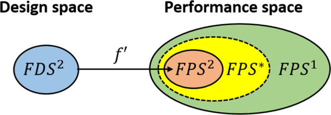
However, $ {y}^{\prime } $
may also be the input variables of some sub-functions. Expanding the ranges of
$ {y}^{\prime } $
may also be the input variables of some sub-functions. Expanding the ranges of $ {y}^{\prime } $
will inevitably lead to the expansion of the input ranges of some sub-functions, which will in turn make the system more difficult or expensive to implement. Therefore, there is an inherent tension between accommodating excessive uncertainty and the level of difficulty in implementing the system. This tension dictates that the boundary of
$ {y}^{\prime } $
will inevitably lead to the expansion of the input ranges of some sub-functions, which will in turn make the system more difficult or expensive to implement. Therefore, there is an inherent tension between accommodating excessive uncertainty and the level of difficulty in implementing the system. This tension dictates that the boundary of $ {FPS}^{\ast } $
in Figure 6 cannot be too close either to
$ {FPS}^{\ast } $
in Figure 6 cannot be too close either to $ {FPS}^1 $
or to
$ {FPS}^1 $
or to $ {FPS}^2 $
.
$ {FPS}^2 $
.
Trade-off Study. A trade-off needs to be made to decide the distance of $ {FPS}^{\ast } $
from
$ {FPS}^{\ast } $
from $ {FPS}^1 $
and
$ {FPS}^1 $
and $ {FPS}^2 $
. This problem highly resembles the barrier function in optimization. Therefore, we construct an optimization problem based on the barrier function to conduct the trade-off study.
$ {FPS}^2 $
. This problem highly resembles the barrier function in optimization. Therefore, we construct an optimization problem based on the barrier function to conduct the trade-off study.
First, we construct the boundaries of the ranges in $ {FPS}^{\ast } $
. For
$ {FPS}^{\ast } $
. For $ {y}_j(i) $
(i.e., the
$ {y}_j(i) $
(i.e., the $ j $
th variable of
$ j $
th variable of $ y(i) $
), let the corresponding range be defined in
$ y(i) $
), let the corresponding range be defined in $ {FPS}^{\ast } $
be
$ {FPS}^{\ast } $
be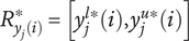 $ {R}_{y_j(i)}^{\ast }=\left[{y}_j^{l\ast }(i),{y}_j^{u\ast }(i)\right] $
. As explained before, the ranges in
$ {R}_{y_j(i)}^{\ast }=\left[{y}_j^{l\ast }(i),{y}_j^{u\ast }(i)\right] $
. As explained before, the ranges in $ {FPS}^{\ast } $
must be bounded by the ranges in
$ {FPS}^{\ast } $
must be bounded by the ranges in $ {FPS}^1 $
and
$ {FPS}^1 $
and $ {FPS}^2 $
. Therefore, the range of
$ {FPS}^2 $
. Therefore, the range of $ {y}_j(i) $
in
$ {y}_j(i) $
in $ {FPS}^{\ast } $
is subject to Eq. (21).
$ {FPS}^{\ast } $
is subject to Eq. (21).
 $$ \left\{\begin{array}{c}{y}_j^{u2}(i)\le {y}_j^{u\ast }(i)\le {y}_j^{u1}(i)\\ {}{y}_j^{l1}(i)\le {y}_j^{l\ast }(i)\le {y}_j^{l2}(i)\end{array}\right. $$
-
•
$ {y}_j^{u1}(i) $
and
$ {y}_j^{l1}(i) $
are the upper and lower bounds of the range of
$ {y}_j(i) $
in
$ {FPS}^1 $
. -
•
$ {y}_j^{u2}(i) $
and
$ {y}_j^{l2}(i) $
are the upper and lower bounds of the range of
$ {y}_j(i) $
in
$ {FPS}^2 $
.


Second, we explain the barrier functions in Eq. (22). $ {y}_j(i) $
is the output of
$ {y}_j(i) $
is the output of $ {f}_i $
. If
$ {f}_i $
. If $ {R}_{y_j(i)}^{\ast } $
is too close to
$ {R}_{y_j(i)}^{\ast } $
is too close to $ {FPS}^2 $
, then
$ {FPS}^2 $
, then $ {h}_j(i) $
goes to infinity. If
$ {h}_j(i) $
goes to infinity. If $ {y}_j(i) $
is the input of
$ {y}_j(i) $
is the input of $ {f}_k $
and
$ {f}_k $
and $ {R}_{y_j(i)}^{\ast } $
is too close to
$ {R}_{y_j(i)}^{\ast } $
is too close to $ {FPS}^1 $
, then
$ {FPS}^1 $
, then $ {h}_j^k(i) $
goes to infinity; otherwise,
$ {h}_j^k(i) $
goes to infinity; otherwise, $ {h}_j^k(i)=0 $
.
$ {h}_j^k(i)=0 $
.
 $$ \left\{\begin{array}{l}{h}_j(i)=-{a}_j(i)\Big(\ln \mid {y}_j^{u\ast }(i)-{y}_j^{u2}(i)\mid \\ {}+\ln \mid {y}_j^{l\ast }(i)-{y}_j^{l2}(i)\mid \Big)\\ {}{h}_j^k(i)=-{a}_j^k(i)\Big(\ln \mid {y}_j^{u\ast }(i)-{y}_j^{u1}(i)\mid \\ {}+\ln \mid {y}_j^{l\ast }(i)-{y}_j^{l1}(i)\mid \Big)\end{array}\right. $$
The coefficients $ {a}_j(i) $
and
$ {a}_j(i) $
and $ {a}_j^k(i) $
represent the designers’ preference for the ability to tolerate uncertainty, expansion of
$ {a}_j^k(i) $
represent the designers’ preference for the ability to tolerate uncertainty, expansion of $ {f}_i $
and the level of difficulty in implementing
$ {f}_i $
and the level of difficulty in implementing $ {f}_k $
. Specific values of
$ {f}_k $
. Specific values of $ {a}_j(i) $
and
$ {a}_j(i) $
and $ {a}_j^k(i) $
can only be determined case by case.
$ {a}_j^k(i) $
can only be determined case by case.
 $$ \min \left(\sum \limits_{i=1}^n\sum \limits_{j=1}^{S(i)}{h}_j(i)+\sum \limits_{i=1}^n\sum \limits_{j=1}^{S(i)}\sum \limits_{k=1}^n{h}_j^k(i)\right) $$
Third, the objective function is Eq. (23), where $ S(i) $
is the number of the variables in
$ S(i) $
is the number of the variables in $ y(i) $
. The optimization problem is to decide
$ y(i) $
. The optimization problem is to decide $ {y}_j^{u\ast }(i) $
and
$ {y}_j^{u\ast }(i) $
and $ {y}_j^{l\ast }(i) $
to minimize Eq. (23), subject to the constraints in Eq. (4) and Eq. (21). As a result,
$ {y}_j^{l\ast }(i) $
to minimize Eq. (23), subject to the constraints in Eq. (4) and Eq. (21). As a result, $ {FPS}^{\ast } $
can be assembled using the resulting
$ {FPS}^{\ast } $
can be assembled using the resulting $ {y}_j^{u\ast }(i) $
and
$ {y}_j^{u\ast }(i) $
and $ {y}_j^{l\ast }(i) $
where
$ {y}_j^{l\ast }(i) $
where $ i=1,2,\dots, n $
.
$ i=1,2,\dots, n $
.
The Sub-Requirements. In general, the sub-requirements must satisfy the following three conditions:
-
1. They must be within the initial feasible spaces of the sub-functions.
-
2. They must include all the possible values that the elements of the system will encounter.
-
3. They must be composable and refine the higher-level functional requirements as a whole.
We intend to assign the ranges in $ {FDS}^2 $
and
$ {FDS}^2 $
and $ {FPS}^{\ast } $
directly to the sub-functions as the sub-requirements. Now, we explain how the ranges satisfy all three conditions above.
$ {FPS}^{\ast } $
directly to the sub-functions as the sub-requirements. Now, we explain how the ranges satisfy all three conditions above.
First, $ {FDS}^1 $
and
$ {FDS}^1 $
and $ {FPS}^1 $
are both narrowed from the initial feasible spaces of the sub-functions (see Eq. (15)), and
$ {FPS}^1 $
are both narrowed from the initial feasible spaces of the sub-functions (see Eq. (15)), and $ {FDS}^2 $
and
$ {FDS}^2 $
and $ {FPS}^{\ast } $
are narrowed from
$ {FPS}^{\ast } $
are narrowed from $ {FDS}^1 $
and
$ {FDS}^1 $
and $ {FPS}^1 $
. Therefore, the ranges in
$ {FPS}^1 $
. Therefore, the ranges in $ {FDS}^2 $
and
$ {FDS}^2 $
and $ {FPS}^{\ast } $
satisfy the first condition.
$ {FPS}^{\ast } $
satisfy the first condition.
Second, $ {FDS}^2 $
does not narrow the ranges of
$ {FDS}^2 $
does not narrow the ranges of $ \left\{x\right\},\left\{\tilde{x}\right\},\left\{u\right\} $
and
$ \left\{x\right\},\left\{\tilde{x}\right\},\left\{u\right\} $
and $ \left\{\tilde{u}\right\} $
, elements that are associated with
$ \left\{\tilde{u}\right\} $
, elements that are associated with $ \forall $
, thus all the values of the independent variables that the system must accept are included within
$ \forall $
, thus all the values of the independent variables that the system must accept are included within $ {FDS}^2 $
. Moreover, we have established in Eq. (20) that all the possible values of
$ {FDS}^2 $
. Moreover, we have established in Eq. (20) that all the possible values of $ {y}^{\prime } $
are included within
$ {y}^{\prime } $
are included within $ {FPS}^2 $
. Because
$ {FPS}^2 $
. Because $ {FPS}^{\ast } $
includes
$ {FPS}^{\ast } $
includes $ {FPS}^2 $
, all the possible values of
$ {FPS}^2 $
, all the possible values of $ {y}^{\prime } $
are also included within
$ {y}^{\prime } $
are also included within $ {FPS}^{\ast } $
. Therefore, the ranges in
$ {FPS}^{\ast } $
. Therefore, the ranges in $ {FDS}^2 $
and
$ {FDS}^2 $
and $ {FPS}^{\ast } $
satisfy the second condition.
$ {FPS}^{\ast } $
satisfy the second condition.
Third, the ranges of all the elements are only defined once in $ {FDS}^2 $
and
$ {FDS}^2 $
and $ {FPS}^{\ast } $
. If they are assigned to the sub-functions, the identical element will only be assigned the same range. Therefore, the sub-requirements will be composable. In addition, the ranges of
$ {FPS}^{\ast } $
. If they are assigned to the sub-functions, the identical element will only be assigned the same range. Therefore, the sub-requirements will be composable. In addition, the ranges of $ \left\{x\right\} $
in
$ \left\{x\right\} $
in $ {FDS}^2 $
are the same as the ranges in the higher-level functional requirements (see Eq. (16)), and the ranges of
$ {FDS}^2 $
are the same as the ranges in the higher-level functional requirements (see Eq. (16)), and the ranges of $ y $
are narrowed from the ranges in the higher-level functional requirements (see Eq. (15)). Therefore, the sub-requirements as a whole will also refine the higher-level functional requirement, and the third condition is satisfied.
$ y $
are narrowed from the ranges in the higher-level functional requirements (see Eq. (15)). Therefore, the sub-requirements as a whole will also refine the higher-level functional requirement, and the third condition is satisfied.
In conclusion, $ {R}_{x(i)}^{\ast },{R}_{c(i)}^{\ast }, $
and
$ {R}_{x(i)}^{\ast },{R}_{c(i)}^{\ast }, $
and $ {R}_{u(i)}^{\ast } $
can be directly obtained from
$ {R}_{u(i)}^{\ast } $
can be directly obtained from $ {FDS}^2 $
, and
$ {FDS}^2 $
, and $ {R}_{y(i)}^{\ast } $
can be directly obtained from
$ {R}_{y(i)}^{\ast } $
can be directly obtained from $ {FPS}^{\ast } $
. Together,
$ {FPS}^{\ast } $
. Together, $ {R}_{x(i)}^{\ast },{R}_{c(i)}^{\ast },{R}_{u(i)}^{\ast }, $
and
$ {R}_{x(i)}^{\ast },{R}_{c(i)}^{\ast },{R}_{u(i)}^{\ast }, $
and $ {R}_{y(i)}^{\ast } $
are the sub-requirements of
$ {R}_{y(i)}^{\ast } $
are the sub-requirements of $ {f}_i $
(
$ {f}_i $
( $ i=1,2,\dots, n $
) decomposed from the
$ i=1,2,\dots, n $
) decomposed from the $ {R}_x^{\ast },{R}_c^{\ast },{R}_u^{\ast }, $
and
$ {R}_x^{\ast },{R}_c^{\ast },{R}_u^{\ast }, $
and $ {R}_y^{\ast } $
of
$ {R}_y^{\ast } $
of $ f $
.
$ f $
.
6. Case study
In this section, we design a cruise control system to demonstrate the four-step formal process proposed in Section 5.
Problem description. The task is to decompose functional requirements for a cruise control system. The top-level function can be represented as a mapping below, where the input is the initial speed $ {v}_0 $
and the reference speed
$ {v}_0 $
and the reference speed $ {v}_r $
; the output is the real speed
$ {v}_r $
; the output is the real speed $ v(t) $
; no uncertainty parameters are defined. Figure 7 is a graphical representation of the mapping.
$ v(t) $
; no uncertainty parameters are defined. Figure 7 is a graphical representation of the mapping.
 $$ ({v}_0,\hskip0.35em {v}_r)\overset{f}{\to }v(t) $$
The requirements are summarized in Table 1: for any initial speed $ {v}_0\in \left[\mathrm{22.0,33.0}\right]\;\mathrm{m}/\mathrm{s} $
and the reference speed
$ {v}_0\in \left[\mathrm{22.0,33.0}\right]\;\mathrm{m}/\mathrm{s} $
and the reference speed $ {v}_r\in \left[\mathrm{34.0,36.0}\right]\;\mathrm{m}/\mathrm{s} $
, the real speed
$ {v}_r\in \left[\mathrm{34.0,36.0}\right]\;\mathrm{m}/\mathrm{s} $
, the real speed $ v(t) $
shall be bounded by
$ v(t) $
shall be bounded by $ \left[\mathrm{20.0,40.0}\right]\;\mathrm{m}/\mathrm{s} $
at all times and converge to
$ \left[\mathrm{20.0,40.0}\right]\;\mathrm{m}/\mathrm{s} $
at all times and converge to $ \left[\mathrm{33.0,37.0}\right]\;\mathrm{m}/\mathrm{s} $
after 20 seconds.
$ \left[\mathrm{33.0,37.0}\right]\;\mathrm{m}/\mathrm{s} $
after 20 seconds.
The top-level function.
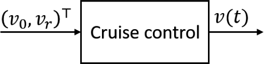
Top-level functional requirements
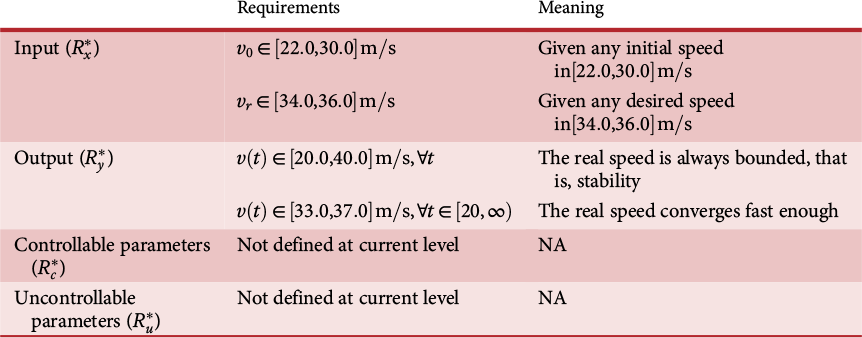
Intuitively, the task of decomposition is breaking down the top-level “box” in Figure 7 into more “boxes” at the lower level (to be explained in Figure 8).
The functional architecture for the top-level functional requirements.
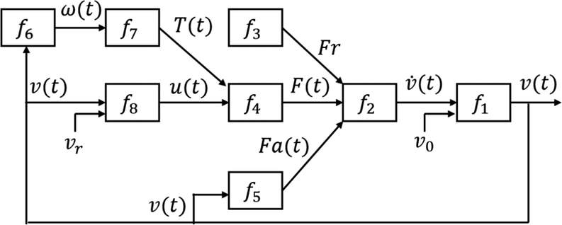
Step 1: Define and analyze the functional architecture. We adopt the functional architecture of a cruise control design from (Aström & Murray Reference Aström and Murray2010) (Figure 8) with each sub-function defined as follows:
 $$ \left(\begin{array}{l}{f}_1:v(t)={\int}_0^t\dot{v}\hskip0.1em dt+{v}_0\\ {}{f}_2:\dot{v}(t)=\frac{F(t)- Fr- Fa(t)}{m}\\ {}{f}_3: Fr={mgC}_r\\ {}{f}_4:F(t)=\alpha \cdot u(t)T(t)\\ {}{f}_5: Fa(t)=\frac{1}{2}\rho {C}_d Av{(t)}^2\\ {}{f}_6:\omega (t)=\alpha \cdot v(t)\\ {}{f}_7:T(t)={T}_m\left(1-\beta {\left(\frac{\omega (t)}{\omega_m}-1\right)}^2\right)\\ {}{f}_8:u(t)=p\left({v}_r-v(t)\right)+i{\int}_0^t\left({v}_r-v(t)\right)\hskip0.1em dt\end{array}\right. $$
Based on the architecture, we derive the design space and the performance of the cruise control system. For example, according to the characterizations in Section 5.2, $ \left\{{y^{\prime}}^{(3)}\right\} $
are the output variables that are defined in the output of the top-level function, the input of the sub-functions, and the output of the sub-functions. The only variable of such we can find is
$ \left\{{y^{\prime}}^{(3)}\right\} $
are the output variables that are defined in the output of the top-level function, the input of the sub-functions, and the output of the sub-functions. The only variable of such we can find is $ v(t) $
, and thus
$ v(t) $
, and thus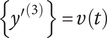 $ \left\{{y^{\prime}}^{(3)}\right\}=v(t) $
. In addition, as defined in Figure 5,
$ \left\{{y^{\prime}}^{(3)}\right\}=v(t) $
. In addition, as defined in Figure 5, $ \left\{{y^{\prime}}^{(1)}\right\} $
and
$ \left\{{y^{\prime}}^{(1)}\right\} $
and $ \left\{{y^{\prime}}^{(4)}\right\} $
are the output variables that are not the inputs to any sub-function. In this example, no
$ \left\{{y^{\prime}}^{(4)}\right\} $
are the output variables that are not the inputs to any sub-function. In this example, no $ \left\{{y^{\prime}}^{(1)}\right\} $
or
$ \left\{{y^{\prime}}^{(1)}\right\} $
or $ \left\{{y^{\prime}}^{(4)}\right\} $
is identified. Moreover, as depicted in Figure 5,
$ \left\{{y^{\prime}}^{(4)}\right\} $
is identified. Moreover, as depicted in Figure 5, $ \left\{\tilde{x}\right\} $
are the variables from the environment but are not defined in the top-level functional requirements. There is no such input variable in the functional architecture in Figure 8. Therefore,
$ \left\{\tilde{x}\right\} $
are the variables from the environment but are not defined in the top-level functional requirements. There is no such input variable in the functional architecture in Figure 8. Therefore, $ \left\{\tilde{x}\right\} $
is empty. Finally, because the uncertain parameters are not defined in the top-level requirements,
$ \left\{\tilde{x}\right\} $
is empty. Finally, because the uncertain parameters are not defined in the top-level requirements, $ \left\{c\right\} $
and
$ \left\{c\right\} $
and $ \left\{u\right\} $
are empty.
$ \left\{u\right\} $
are empty.
-
•
$ \left\{x\right\}=\left\{{v}_r,{v}_0\right\} $
. -
•
$ \left\{\tilde{c}\right\}=\left\{{\omega}_m\right\} $
. -
•
$ \left\{\tilde{u}\right\}=\left\{m\right\} $
. -
•
$ \left\{{y^{\prime}}^{(2)}\right\}=\left\{\dot{v}(t), Fr(t),F(t), Fa(t),T(t),u(t),\omega (t)\right\} $
. -
•
$ \left\{{y^{\prime}}^{(3)}\right\}=v(t) $
.




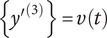
As a result, according to Eq. (12), the design space of the cruise control system is, $ \left\{{v}_r,{v}_0,m,{\omega}_m\right\} $
and the performance space of the cruise control system is, $ \left\{\dot{v}(t), Fr(t),F(t), Fa(t),T(t),u(t),\omega (t),v(t)\right\}. $
Step 2: Explore the initial feasible spaces. The characterizations of the sub-functions depend on the feasible implementations of the respective sub-function, which can only be determined case by case. For this example, we characterize each sub-function of the functional architecture in Figure 8 as below: $ {\mathbf{f}}_{\mathbf{1}} $
is a mathematical definition of the speed, and hence will be allocated to no subsystem.
$ {\mathbf{f}}_{\mathbf{1}} $
is a mathematical definition of the speed, and hence will be allocated to no subsystem. $ \dot{v}(t) $
has to be bounded to avoid violent acceleration/deceleration by the cruise control;
$ \dot{v}(t) $
has to be bounded to avoid violent acceleration/deceleration by the cruise control; $ v(t) $
is bounded to constrain the fastest speed at which the cruise control can be engaged due to safety concerns.
$ v(t) $
is bounded to constrain the fastest speed at which the cruise control can be engaged due to safety concerns.
-
•
$ {f}_1 $
:
$ v(t)={\int}_0^t\dot{v} dt+{v}_0 $
. -
•
$ x(1)={\left({v}_0,\dot{v}\right)}^{\top } $
and,

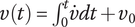
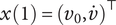
 $$ {R}_{x(1)}={\left(\left[0,40\right]\mathrm{m}/\mathrm{s},\left[-\mathrm{1.5,3}\right]\mathrm{m}/{\mathrm{s}}^2\right)}^{\top }. $$
-
•
$ y(1)=v(t) $
and
$ {R}_{y(1)}=\left[0,50\right]\mathrm{m}/\mathrm{s} $
.

 $ {\mathbf{f}}_{\mathbf{2}} $
combines all the forces and yields the acceleration of the car as a whole, where
$ {\mathbf{f}}_{\mathbf{2}} $
combines all the forces and yields the acceleration of the car as a whole, where $ F(t) $
is the driving force,
$ F(t) $
is the driving force, $ Fa(t) $
is the aerodynamic drag and
$ Fa(t) $
is the aerodynamic drag and $ Fr $
is the tyre friction. The weight of the car
$ Fr $
is the tyre friction. The weight of the car $ m $
is defined as an uncontrollable parameter.
$ m $
is defined as an uncontrollable parameter.
-
•
$ {f}_2 $
:
$ \dot{v}(t)=\left(F(t)- Fr- Fa(t)\right)/m $
. -
•
$ x(2)={\left(F(t), Fr, Fa(t)\right)}^{\top } $
and,



 $$ {R}_{x(2)}={\left(\left[-250,3500\right]\mathrm{N},\left[\mathrm{60,130}\right]\mathrm{N},\left[0,1000\right]\mathrm{N}\right)}^{\top }. $$
-
•
$ y(2)=\dot{v}(t) $
and
$ {R}_{y(2)}=\left[-2,4\right]\mathrm{m}/{\mathrm{s}}^2 $
; -
•
$ u(2)=m $
and
$ {R}_{u(2)}=\left[990,1100\right]\mathrm{kg} $
.



 $ {\mathbf{f}}_{\mathbf{3}} $
represent the rolling friction of the tyre. No input is defined for this function.
$ {\mathbf{f}}_{\mathbf{3}} $
represent the rolling friction of the tyre. No input is defined for this function. $ {C}_r $
is the rolling friction coefficient.
$ {C}_r $
is the rolling friction coefficient.
-
•
$ {f}_3 $
:
$ Fr={mgC}_r $
. -
•
$ y(3)= Fr $
and
$ {R}_{y(3)}=\left[\mathrm{70,120}\right]\mathrm{N} $
. -
•
$ u(3)=m $
and
$ {R}_{u(3)}=\left[990,1100\right]\mathrm{kg} $
.




 $ {\mathbf{f}}_{\mathbf{4}} $
represents the ability of the drivetrain to convert the torque to the driving force, where
$ {\mathbf{f}}_{\mathbf{4}} $
represents the ability of the drivetrain to convert the torque to the driving force, where $ \alpha $
is the gear ratio,
$ \alpha $
is the gear ratio, $ u(t) $
is the control input from the cruise controller (not the uncontrollable uncertain parameters defined in this paper),
$ u(t) $
is the control input from the cruise controller (not the uncontrollable uncertain parameters defined in this paper), $ T(t) $
is the torque.
$ T(t) $
is the torque.
-
•
$ {f}_4 $
:
$ F(t)=\alpha \ast u(t)T(t) $
. -
•
$ x(4)={\left(u(t),T(t)\right)}^{\top } $
and,



 $$ {R}_{x(4)}={\left(\left[-\mathrm{0.5,2}\right],\left[\mathrm{0,250}\right]\mathrm{N}\cdot \mathrm{m}\right)}^{\top }. $$
-
•
$ y(4)=F(t) $
and
$ {R}_{y(4)}=\left[-1250,5000\right]\mathrm{N} $
.

 $ {\mathbf{f}}_{\mathbf{5}} $
represents the aerodynamic drag, where
$ {\mathbf{f}}_{\mathbf{5}} $
represents the aerodynamic drag, where $ \rho $
is the air density,
$ \rho $
is the air density, $ {C}_d $
is the shape-dependent aerodynamic drag coefficient and
$ {C}_d $
is the shape-dependent aerodynamic drag coefficient and $ A $
is the frontal area of the car.
$ A $
is the frontal area of the car.
-
•
$ {f}_5 $
:
$ Fa(t)=\frac{1}{2}\rho {C}_d Av{(t)}^2 $
; -
•
$ x(5)=v(t) $
and
$ {R}_{x(5)}=\left[0,60\right]\mathrm{m}/\mathrm{s} $
. -
•
$ y(5)= Fa(t) $
and
$ {R}_{y(5)}=\left[0,2000\right]\mathrm{N} $
.




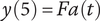
 $ {\mathbf{f}}_{\mathbf{6}} $
represents the ability of the drivetrain to convert from the car speed
$ {\mathbf{f}}_{\mathbf{6}} $
represents the ability of the drivetrain to convert from the car speed $ v(t) $
to the engine speed
$ v(t) $
to the engine speed $ \omega (t) $
.
$ \omega (t) $
.
-
•
$ {f}_6 $
:
$ \omega (t)=\alpha \ast v(t) $
; -
•
$ x(6)=v(t) $
and
$ {R}_{x(6)}=\left[0,55\right]\mathrm{m}/\mathrm{s} $
. -
•
$ y(6)=\omega (t) $
and
$ {R}_{y(6)}=\left[\mathrm{0,560}\right]\mathrm{rad}/\mathrm{s} $
.





 $ {\mathbf{f}}_{\mathbf{7}} $
represents the correlation between the torque, the engine speed
$ {\mathbf{f}}_{\mathbf{7}} $
represents the correlation between the torque, the engine speed $ \omega (t) $
, the maximum torque
$ \omega (t) $
, the maximum torque $ {T}_m $
and the maximum engine speed
$ {T}_m $
and the maximum engine speed $ {\omega}_m $
.
$ {\omega}_m $
. $ {\omega}_m $
is the controllable uncertain design parameter that starts with a rough estimation but will eventually be determined by the designers.
$ {\omega}_m $
is the controllable uncertain design parameter that starts with a rough estimation but will eventually be determined by the designers.
-
•
$ {f}_7 $
:
$ T(t)={T}_m\left(1-\beta {\left(\omega (t)/{\omega}_m-1\right)}^2\right) $
. -
•
$ x(7)=\omega (t) $
and
$ {R}_{x(7)}=\left[\mathrm{0,450}\right]\mathrm{rad}/\mathrm{s} $
. -
•
$ y(7)=T(t) $
and
$ {R}_{y(7)}=\left[\mathrm{0,250}\right] $
NM. -
•
$ c(7)={\omega}_m $
and
$ {R}_{c(7)}=\left[\mathrm{350,480}\right]\mathrm{rad}/\mathrm{s} $
.





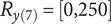

 $ {\mathbf{f}}_{\mathbf{8}} $
is the cruise controller, in this case, based on PID control.
$ {\mathbf{f}}_{\mathbf{8}} $
is the cruise controller, in this case, based on PID control. $ p $
and
$ p $
and $ i $
are the proportional and integral parameters for the PID controller.
$ i $
are the proportional and integral parameters for the PID controller.
-
•
$ {f}_8 $
:
$ u(t)=p\left({v}_r-v(t)\right)+i{\int}_0^t\left({v}_r-v(t)\right) dt $
. -
•
$ x(8)={\left({v}_r,v(t)\right)}^{\top } $
and,



 $$ {R}_{x(8)}={\left(\left[0,60\right]\mathrm{m}/\mathrm{s},\left[0,60\right]\mathrm{m}/\mathrm{s}\right)}^{\top }. $$
-
•
$ y(8)=u(t) $
and
$ {R}_{y(8)}=\left[-\mathrm{0.5,4}\right] $
.


The coefficients mentioned above are $ \alpha =10,g=9.8,{C}_r=0.01,{C}_d=0.32,\rho =1.3,A=2.4,\beta =0.4,{T}_m=200,p=0.1,i=0.5 $
. Note that these constant coefficients can also be defined as uncertain parameters, just like
$ \alpha =10,g=9.8,{C}_r=0.01,{C}_d=0.32,\rho =1.3,A=2.4,\beta =0.4,{T}_m=200,p=0.1,i=0.5 $
. Note that these constant coefficients can also be defined as uncertain parameters, just like $ m $
and
$ m $
and $ {\omega}_m $
, which will make the computation more challenging. However, we intentionally limit the number of uncertain parameters to simplify the presentation.
$ {\omega}_m $
, which will make the computation more challenging. However, we intentionally limit the number of uncertain parameters to simplify the presentation.
Step 3: Narrow the feasible spaces. First, we compute $ {FDS}^1 $
and
$ {FDS}^1 $
and $ {FPS}^1 $
by taking intersections of the ranges of the elements defined in multiple places. For example,
$ {FPS}^1 $
by taking intersections of the ranges of the elements defined in multiple places. For example, $ m $
is defined in
$ m $
is defined in $ {f}_2 $
and
$ {f}_2 $
and $ {f}_3 $
, hence
$ {f}_3 $
, hence $ {R}_m $
is the intersection of the corresponding ranges defined in
$ {R}_m $
is the intersection of the corresponding ranges defined in $ {f}_2 $
and
$ {f}_2 $
and $ {f}_3 $
.
$ {f}_3 $
. $ {v}_0 $
is defined in both the top-level function and
$ {v}_0 $
is defined in both the top-level function and $ {f}_1 $
, hence
$ {f}_1 $
, hence $ {R}_{v_0} $
is the intersection of the corresponding ranges defined in
$ {R}_{v_0} $
is the intersection of the corresponding ranges defined in $ {f}_1 $
and the top-level function.
$ {f}_1 $
and the top-level function.
As a result, the ranges in $ {FDS}^1 $
can be computed as follows:
$ {FDS}^1 $
can be computed as follows: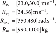 $ {\displaystyle \begin{array}{c}{R}_{v_r}=\left[\mathrm{23.0,30.0}\right]\;\mathrm{m}\;{\mathrm{s}}^{-1},\\ {}{R}_{v_0}=\left[34,36\right]\;\mathrm{m}\;{\mathrm{s}}^{-1},\\ {}{R}_{\omega_m}=\left[\mathrm{350,480}\right]\;\mathrm{rad}\;{\mathrm{s}}^{-1},\\ {}{R}_m=\left[990,1100\right]\;\mathrm{kg}\end{array}} $
The ranges in $ {FPS}^1 $
can be computed as follows:
$ {FPS}^1 $
can be computed as follows: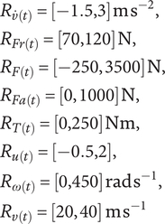 $ {\displaystyle \begin{array}{l}{R}_{\dot{v}(t)}=\left[-\mathrm{1.5,3}\right]\;\mathrm{m}\;{\mathrm{s}}^{-2},\\ {}{R}_{Fr(t)}=\left[\mathrm{70,120}\right]\;\mathrm{N},\\ {}{R}_{F(t)}=\left[-250,3500\right]\;\mathrm{N},\\ {}{R}_{Fa(t)}=\left[0,1000\right]\;\mathrm{N},\\ {}{R}_{T(t)}=\left[\mathrm{0,250}\right]\;\mathrm{N}\mathrm{m},\\ {}{R}_{u(t)}=\left[-\mathrm{0.5,2}\right],\\ {}{R}_{\omega (t)}=\left[\mathrm{0,450}\right]\;\mathrm{rad}\;{\mathrm{s}}^{-1},\\ {}{R}_{v(t)}=\left[20,40\right]\hskip0.22em \mathrm{m}\;{\mathrm{s}}^{-1}\end{array}} $
Second, let $ {f}^{\prime }={f}_1\wedge {f}_2\wedge \dots \wedge {f}_8 $
.
$ {f}^{\prime }={f}_1\wedge {f}_2\wedge \dots \wedge {f}_8 $
. $ {FDS}^1 $
and
$ {FDS}^1 $
and $ {FPS}^1 $
can be further narrowed into
$ {FPS}^1 $
can be further narrowed into $ {FDS}^2 $
and
$ {FDS}^2 $
and $ {FPS}^2 $
using
$ {FPS}^2 $
using $ {f}^{\prime } $
. To achieve
$ {f}^{\prime } $
. To achieve $ {FDS}^2 $
, the range of the controllable parameter
$ {FDS}^2 $
, the range of the controllable parameter $ {\omega}_m $
must be narrowed into
$ {\omega}_m $
must be narrowed into $ {R}_{\omega_m}^{\downarrow } $
based on Eq. (19) such that,
$ {R}_{\omega_m}^{\downarrow } $
based on Eq. (19) such that,
 $$ \mathrm{For}\hskip0.5em \forall {v}_r\in {R}_{v_r},\forall {v}_0\in {R}_{v_0},\forall m\in {R}_m,\forall {\omega}_m\in {R}_{\omega_m}^{\downarrow }:\left({v}_r,{v}_0,{\omega}_m,m\right)\overset{f^{\prime }}{\to }{y}^{\prime}\in {FPS}^1 $$
where $ {y}^{\prime }={\left(v(t),\dot{v}(t), Fr(t),F(t), Fa(t),T(t),u(t),\omega (t)\right)}^{\top } $
. In this example, we apply reachability analysis to help find
$ {y}^{\prime }={\left(v(t),\dot{v}(t), Fr(t),F(t), Fa(t),T(t),u(t),\omega (t)\right)}^{\top } $
. In this example, we apply reachability analysis to help find $ {R}_{\omega_m}^{\downarrow } $
. We estimate an over-approximation of
$ {R}_{\omega_m}^{\downarrow } $
. We estimate an over-approximation of $ {R}_{\omega_m}^{\downarrow } $
, feed it into a reachability solver (i.e., CORA (Althoff Reference Althoff2015) in this example), and adjust the bounds of the over-approximation until the reachable sets of all the output variables are bounded within
$ {R}_{\omega_m}^{\downarrow } $
, feed it into a reachability solver (i.e., CORA (Althoff Reference Althoff2015) in this example), and adjust the bounds of the over-approximation until the reachable sets of all the output variables are bounded within $ {FPS}^1 $
.
$ {FPS}^1 $
.
As a result, we obtain the ranges in $ {FDS}^2 $
as follows:
$ {FDS}^2 $
as follows: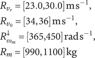 $ {\displaystyle \begin{array}{l}{R}_{v_r}=\left[\mathrm{23.0,30.0}\right]\;\mathrm{m}\;{\mathrm{s}}^{-1},\\ {}{R}_{v_0}=\left[34,36\right]\;\mathrm{m}\;{\mathrm{s}}^{-1},\\ {}{R}_{\omega_m}^{\downarrow }=\left[\mathrm{365,450}\right]\;\mathrm{rad}\;{\mathrm{s}}^{-1},\\ {}{R}_m=\left[990,1100\right]\;\mathrm{kg}\end{array}} $
After that, $ {FPS}^1 $
can be narrowed into
$ {FPS}^1 $
can be narrowed into $ {FPS}^2 $
by calculating the reachable sets according to Eq. (20). We choose CORA as the tool because it can compute the over-approximation of the feasible performance space. The result shows the range of
$ {FPS}^2 $
by calculating the reachable sets according to Eq. (20). We choose CORA as the tool because it can compute the over-approximation of the feasible performance space. The result shows the range of $ v(t) $
converges gradually from
$ v(t) $
converges gradually from $ {R}_{v_0} $
to
$ {R}_{v_0} $
to $ {R}_{v_r} $
, meaning the reference speed is achieved by the cruise control system. Eventually, we obtain the ranges of
$ {R}_{v_r} $
, meaning the reference speed is achieved by the cruise control system. Eventually, we obtain the ranges of $ {FPS}^2 $
:
$ {FPS}^2 $
: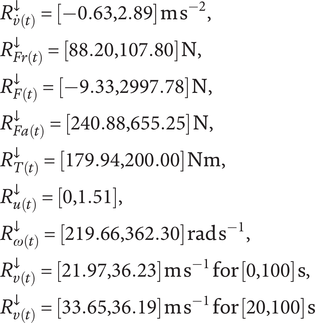 $ {\displaystyle \begin{array}{l}{R}_{\dot{v}(t)}^{\downarrow }=\left[-\mathrm{0.63,2.89}\right]\;\mathrm{m}\;{\mathrm{s}}^{-2},\\ {}{R}_{Fr(t)}^{\downarrow }=\left[\mathrm{88.20,107.80}\right]\;\mathrm{N},\\ {}{R}_{F(t)}^{\downarrow }=\left[-\mathrm{9.33,2997.78}\right]\;\mathrm{N},\\ {}{R}_{Fa(t)}^{\downarrow }=\left[\mathrm{240.88,655.25}\right]\;\mathrm{N},\\ {}{R}_{T(t)}^{\downarrow }=\left[\mathrm{179.94,200.00}\right]\;\mathrm{N}\mathrm{m},\\ {}{R}_{u(t)}^{\downarrow }=\left[\mathrm{0,1.51}\right],\\ {}{R}_{\omega (t)}^{\downarrow }=\left[\mathrm{219.66,362.30}\right]\;\mathrm{rad}\;{\mathrm{s}}^{-1},\\ {}{R}_{v(t)}^{\downarrow }=\left[\mathrm{21.97,36.23}\right]\;\mathrm{m}\;{\mathrm{s}}^{-1}\;\mathrm{for}\;\left[\mathrm{0,100}\right]\;\mathrm{s},\\ {}{R}_{v(t)}^{\downarrow }=\left[\mathrm{33.65,36.19}\right]\;\mathrm{m}\;{\mathrm{s}}^{-1}\;\mathrm{for}\;\left[\mathrm{20,100}\right]\;\mathrm{s}\end{array}} $
All the ranges in $ {FPS}^2 $
are subsets of their counterparts in
$ {FPS}^2 $
are subsets of their counterparts in $ {FPS}^1 $
. In other words,
$ {FPS}^1 $
. In other words, $ {FPS}^2 $
is successfully narrowed from
$ {FPS}^2 $
is successfully narrowed from $ {FPS}^1 $
.
$ {FPS}^1 $
.
Step 4: Determine the sub-requirements. We compute $ {R}_{y(i)}^{\ast }=\left[{y}^{l\ast }(i),{y}^{u\ast }(i)\right] $
for
$ {R}_{y(i)}^{\ast }=\left[{y}^{l\ast }(i),{y}^{u\ast }(i)\right] $
for $ y(i) $
(
$ y(i) $
( $ i=1,2,\dots, 8 $
) by formulating the optimization problem in Eq. (23) subject to the constraints in Eq. (4) and Eq. (21). Note that there is no subscript
$ i=1,2,\dots, 8 $
) by formulating the optimization problem in Eq. (23) subject to the constraints in Eq. (4) and Eq. (21). Note that there is no subscript $ j $
associated with the output variable
$ j $
associated with the output variable $ y(i) $
, because each
$ y(i) $
, because each $ {f}_i $
in this example only has one variable at its output side.
$ {f}_i $
in this example only has one variable at its output side.
First, the constraints described in Eq. (21) can be directly obtained from $ {FDS}^1,{FPS}^1,{FDS}^2 $
and
$ {FDS}^1,{FPS}^1,{FDS}^2 $
and $ {FPS}^2 $
calculated in the previous step.
$ {FPS}^2 $
calculated in the previous step.
Second, Eq. (4) needs to be satisfied for each individual sub-function, which yields the constraints in Eq. (24). Note that $ {f}_1 $
and
$ {f}_1 $
and $ {f}_8 $
are not included in the constraints.
$ {f}_8 $
are not included in the constraints. $ {f}_1 $
and
$ {f}_1 $
and $ {f}_8 $
alone are not enough to decide the ranges of the output variables because the operation
$ {f}_8 $
alone are not enough to decide the ranges of the output variables because the operation $ \int $
makes the ranges of the output variables correlated with the time
$ \int $
makes the ranges of the output variables correlated with the time $ t $
. Their ranges can only be determined after the rest of the system is determined. In this example,
$ t $
. Their ranges can only be determined after the rest of the system is determined. In this example, $ {f}_1 $
and
$ {f}_1 $
and $ {f}_8 $
belong to the PID controller. These modules are designed after other parts of the car (e.g., engine and tires) are defined, and hence are not part of the constraints in Eq. (24).
$ {f}_8 $
belong to the PID controller. These modules are designed after other parts of the car (e.g., engine and tires) are defined, and hence are not part of the constraints in Eq. (24).
 $$ \left(\begin{array}{l}{y}^{l\ast }(6)\le {f}_6\left({y}^{l\ast }(1)\right)\\ {}{y}^{u\ast }(6)\ge {f}_6\left({y}^{u\ast }(1)\right)\\ {}{y}^{l\ast }(7)\le {f}_7\left({y}^{l\ast }(6),\overline{\omega_m}\right)\\ {}{y}^{u\ast }(7)\ge {f}_7\left({y}^{u\ast }(6),\underline {\omega_m}\right)\\ {}{y}^{l\ast }(5)\le {f}_5\left({y}^{l\ast }(1)\right)\\ {}{y}^{u\ast }(5)\ge {f}_5\left({y}^{u\ast }(1)\right)\\ {}{y}^{l\ast }(4)\le {f}_4\left({y}^{l\ast }(7),{y}^{l\ast }(8)\right)\\ {}{y}^{u\ast }(4)\ge {f}_4\left({y}^{u\ast }(7),{y}^{u\ast }(8)\right)\\ {}{y}^{l\ast }(2)\le {f}_2\left({y}^{l\ast }(4),{y}^{u\ast }(3),{y}^{u\ast }(5),\overline{m}\right)\\ {}{y}^{u\ast }(2)\ge {f}_2\left({y}^{u\ast }(4),{y}^{l\ast }(3),{y}^{l\ast }(5),\underline{m}\right)\end{array}\right. $$
Third, based on Eq. (22) and Eq. (23), we define the objective function below:
 $$ \min \left(\sum \limits_{i=1}^8h(i)+\sum \limits_{i=1}^8\sum \limits_{k=1}^8{h}^k(i)\right) $$
where the coefficients are defined as $ a(1)=0.9,a(2)=0.6,a(3)=0.5,a(4)=0.3,a(5)=0.4, $ $ a(6)=0.5,a(7)=0.1,a(8)=0.9,{a}^5(1)=0.5,{a}^6(1)=0.1,{a}^8(1)=0.8,{a}^1(2)=0.6,{a}^2(3)=0.4, $ $ {a}^2(4)=0.8,{a}^2(5)=0.7,{a}^7(6)=0.6,{a}^4(7)=0.9,{a}^4(8)=0.9 $
.
$ {a}^2(4)=0.8,{a}^2(5)=0.7,{a}^7(6)=0.6,{a}^4(7)=0.9,{a}^4(8)=0.9 $
.
Finally, the optimization problem is to decide $ {y}^{u\ast }(i) $
and
$ {y}^{u\ast }(i) $
and $ {y}^{l\ast }(i) $
(
$ {y}^{l\ast }(i) $
( $ i=1,2,\dots, 8 $
) by minimizing Eq. (25). As a result,
$ i=1,2,\dots, 8 $
) by minimizing Eq. (25). As a result, $ {y}^{u\ast }(i) $
and
$ {y}^{u\ast }(i) $
and $ {y}^{l\ast }(i) $
(
$ {y}^{l\ast }(i) $
( $ i=1,2,\dots, 8 $
) are calculated. Together with
$ i=1,2,\dots, 8 $
) are calculated. Together with $ {FDS}^2 $
computed in the previous step, the ranges of each sub-function can be summarized in Table 2. Accordingly, the sub-requirements of
$ {FDS}^2 $
computed in the previous step, the ranges of each sub-function can be summarized in Table 2. Accordingly, the sub-requirements of $ {f}_i $
are the mapping between
$ {f}_i $
are the mapping between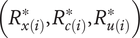 $ \left({R}_{x(i)}^{\ast },{R}_{c(i)}^{\ast },{R}_{u(i)}^{\ast}\right) $
and
$ \left({R}_{x(i)}^{\ast },{R}_{c(i)}^{\ast },{R}_{u(i)}^{\ast}\right) $
and $ {R}_{y(i)}^{\ast } $
in Table 2.
$ {R}_{y(i)}^{\ast } $
in Table 2.
The requirements of the sub-functions
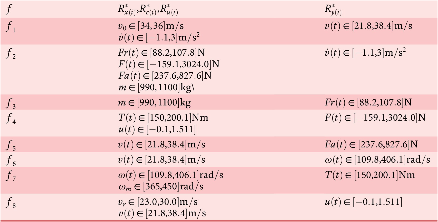
Figure 9 is a graphical representation of the results. The top-level function $ f $
is decomposed into eight sub-functions
$ f $
is decomposed into eight sub-functions $ {f}_1,{f}_2,\dots, {f}_8 $
. As a whole, the eight functions have the same input variables and output variables as the top-level function. Other input variables of the sub-functions can be found at the outputs of the sub-functions, and vice versa. As we can see in Table 2, the variables that appear at both the input side and the output side have the same ranges, meaning the sub-functions are composable. Furthermore, the sub-functions as a whole refine
$ {f}_1,{f}_2,\dots, {f}_8 $
. As a whole, the eight functions have the same input variables and output variables as the top-level function. Other input variables of the sub-functions can be found at the outputs of the sub-functions, and vice versa. As we can see in Table 2, the variables that appear at both the input side and the output side have the same ranges, meaning the sub-functions are composable. Furthermore, the sub-functions as a whole refine $ f $
because the input sets of the former include no less elements than the latter and the output set includes no more elements than the former. Based on our findings of parallel development in Section 4, these sub-functions can be implemented independently. The same process can be repeated to further decompose the sub-functions at even lower levels, which eventually will lead to a system that satisfies the top-level functional requirements.
$ f $
because the input sets of the former include no less elements than the latter and the output set includes no more elements than the former. Based on our findings of parallel development in Section 4, these sub-functions can be implemented independently. The same process can be repeated to further decompose the sub-functions at even lower levels, which eventually will lead to a system that satisfies the top-level functional requirements.
A graphical representation of the results.

7. Conclusion
7.1. Summary
Functional requirements decomposition at the early stage is challenging due to the uncertainty and ambiguity in design and the loose inter-team coordination, especially in large projects for complex systems (e.g., commercial airlines). SBD has demonstrated excellent potential in addressing these challenges, but with limited formal guidance. To tackle uncertainty and ambiguity, one of the most effective approaches is to formalize. SBD’s claim for team autonomy lacks formal proof as well. For this reason, this paper formalizes the functional requirements decomposition process based on SBD principles. We first prove parallel development: as long as the sub-requirements are composable and refine the higher-level functional requirements, the design teams at multiple levels can decompose their functional requirements independently, and the final system will still satisfy the top-level functional requirements. After that, we propose a four-step formal process that supports parallel development to decompose the functional requirements based on SBD principles. Finally, a case study on designing a cruise control system was conducted to demonstrate the effectiveness of the proposed approach.
7.2. Discussion
Toyota’s process. According to Specking et al., much of the SBD literature shares similar characteristics with Toyota’s process (Specking et al. Reference Specking, Whitcomb, Parnell, Goerger, Pohl and Kundeti2018a). We compare our process with Toyota’s approach below. In Toyota’s approach (Ward et al. Reference Ward, Liker, Cristiano and Sobek1995):
-
1. The team defines a set of solutions at the system level.
-
2. It defines sets of possible solutions for various subsystems.
-
3. It explores these possible subsystems in parallel to characterize a possible set of solutions.
-
4. It gradually narrows the set of solutions, converging slowly toward a single solution. In particular, the team determines the appropriate specifications to impose on the subsystems.
-
5. Once the team establishes the single solution for any part of the design, it does not change it unless absolutely necessary.
The first step above is the same as Step 1 in our process, where the “solution” in our case is the functional architecture. The second and third steps above correspond to Step 2 of our process, which essentially involves defining the feasible implementation of the subsystems individually. The fourth step above corresponds to Steps 3 and 4 in our process. However, our formal process provides more details without ambiguity. With the underlying formalism defined in the process, we can explain how to narrow the sets, determine the specifications on the subsystems, and gradually converge to a single solution using hierarchy. The fifth step above is related to the uncertainty expansion addressed in our process. Specifically, Toyota applies “rigorous effort to avoid changes that expand, rather than contract, the space of possible designs” (Ward et al. Reference Ward, Liker, Cristiano and Sobek1995). We believe expansion is sometimes unavoidable due to epistemic uncertainties. Step 4 of our process for “uncertainty expansion” is motivated by this reason and designed to address the possible impacts of unexpected uncertainty expansions.
Implication for design. Requirements decomposition is not a stand-alone activity in design. It is inherently multidisciplinary, integrating principles from systems engineering, software development, human factors and organizational behavior. Our approach makes positive implications for the overall design by addressing the following four concerns while the design is progressing to one level lower: (1) the sub-requirements must not be technically too demanding, making them infeasible or too expensive to implement, (2) the sub-requirements must not be too limited, failing to support the intended system-level function and performance, (3) the sub-requirements must not be too relaxed, wasting too much capability of the subsystems and (4) the sub-requirements should not be too tight, leaving little room for uncertainty. Traditionally, addressing these concerns requires intense communication efforts and conflict resolution between various stakeholders. Our approach solves them with a formal framework, increasing communication efficiency, directing conflict resolution and ensuring successful integration with mathematical rigor. However, it is worth noting that formalism is by no means a silver bullet for solve all the challenges in requirements decomposition. Our approach should be blended with other activities (e.g., requirements negotiation and change management) and methods (e.g., optimization and reachability analysis) to eventually achieve a more effective and efficient requirements decomposition process.
Scope. Our approach enhances requirements decomposition, but does not solve all the challenges in requirements decomposition. First, requirements decomposition entails much more equally important topics than those presented in this paper, such as requirements elicitation, architecture definition and requirements validation and verification. This paper sets itself apart by focusing on addressing the four concerns discussed above. In the future, we will seek to understand how to integrate our approach with other equally important topics to further advance the research on requirements decomposition. Second, the proposed four-step process is a framework that focuses on articulating what needs to be solved rather than how to solve them. Multiple computational problems (e.g., optimization) are identified and formally defined without specifying the methods and tools to solve them and prescribing how well they need to be solved. Such ambiguity is left on purpose because (1) these computational problems on their own are still very active research topics, and (2) we intend to leave the most autonomy to the design teams to decide how to solve these problems with what tools. For this reason, we intentionally downplay the computational analysis (e.g., complexity analysis) in the paper as they are not directly relevant to addressing the four concerns discussed above and depend on the specific methods and tools selected by the engineers. We do not claim a contribution to the computational aspect of the proposed process. Finally, formalism means precision but does not remove engineer’s judgment out of the equation. Formalism in our framework instills precision in the decomposition process and reduces communication efforts by eliminating conflicts with the formally defined procedural requirements in place. But engineer’s judgment are still required as input. For example, the coefficients of the barrier function in Eq. (22) reflect engineer’s tolerance for uncertainty expansion and their evaluation of the level of difficulty in implementing the sub-requirements. Determining these coefficients is highly subjective, same as many other optimization problems that involve human subjective inputs. We do not study how these coefficients are determined in this paper, but will explore the underlying decision-making mechanism in the future.
Managing complexity. A complex system usually has hundreds, if not thousands, of functions. Such a level of complexity is a main challenge for designing modern systems. As a solution, abstraction is one of the most effective tools to manage complexity (Hill et al. Reference Hill, Houle, Merritt and Stix2008; Bencomo et al. Reference Bencomo, Cabot, Chechik, Cheng, Combemale and Zschaler2024). The activity of decomposition, on one hand, refines the higher-level abstraction, and on the other hand, creates abstractions for the lower-level system. The reason for applying abstraction is that there is a limit to human cognitive manageability. It is recommended by multiple systems engineering handbooks (Kapurch Reference Kapurch2010; INCOSE 2023) that decomposition should maintain a reasonable number of functions per level. This number is generally aligned with the famous Miller’s law (Miller Reference Miller1956: 5–9) functions per level, which is also the choice of the cruise control case study in this paper. Furthermore, the proposed process is agnostic to the number of sub-functions abstracted per level. The sub-functions can be further decomposed into multiple levels of smaller components. In fact, the deep hierarchical abstraction of the complex system makes the SBD-based method a particularly suitable approach to requirements decomposition.
Margin. As mentioned before, many concepts incorporated in this paper are closely related to margin. First, in Eq. (2), $ u $
denotes the uncertain parameters that cannot be controlled with
$ u $
denotes the uncertain parameters that cannot be controlled with $ {R}_u^{\ast } $
as a quantification of the uncertainty. While the uncertainty might be reduced due to, for example, a better understanding of the system and the environment,
$ {R}_u^{\ast } $
as a quantification of the uncertainty. While the uncertainty might be reduced due to, for example, a better understanding of the system and the environment, $ \forall u\in {R}_u^{\ast } $
instills a margin (more precisely, buffer) into the system design at the current level that no matter whether and how the uncertainty is reduced, the uncertainty can always be absorbed by the design. Second, the
$ \forall u\in {R}_u^{\ast } $
instills a margin (more precisely, buffer) into the system design at the current level that no matter whether and how the uncertainty is reduced, the uncertainty can always be absorbed by the design. Second, the $ \in $
in Eq. (2) ensures that all the output values generated from the inputs and parameters can be successfully processed by the system, creating a margin (more precisely, excess) for the system output. Third,
$ \in $
in Eq. (2) ensures that all the output values generated from the inputs and parameters can be successfully processed by the system, creating a margin (more precisely, excess) for the system output. Third, $ c $
and
$ c $
and $ \tilde{c} $
of Eq. (19) are controllable parameters, which are associated with
$ \tilde{c} $
of Eq. (19) are controllable parameters, which are associated with $ \exists $
in the original system formulation in Eq. (2). But the narrowed bounds
$ \exists $
in the original system formulation in Eq. (2). But the narrowed bounds $ {R}_c^{\downarrow } $
and
$ {R}_c^{\downarrow } $
and $ {R}_{\tilde{c}}^{\downarrow } $
in Eq. (19) are associated with
$ {R}_{\tilde{c}}^{\downarrow } $
in Eq. (19) are associated with $ \forall $
. This is because
$ \forall $
. This is because $ c $
and
$ c $
and $ \tilde{c} $
will be further narrowed at the lower level of abstraction.
$ \tilde{c} $
will be further narrowed at the lower level of abstraction. $ \forall $
provides a margin (more precisely, buffer) for the lower levels, so that no matter how
$ \forall $
provides a margin (more precisely, buffer) for the lower levels, so that no matter how $ c $
and
$ c $
and $ \tilde{c} $
are decided at a later time, it will never cause a violation at the higher level. Fourth,
$ \tilde{c} $
are decided at a later time, it will never cause a violation at the higher level. Fourth, $ {FPS}^2 $
is computed in Eq. (20) as an over-approximation of
$ {FPS}^2 $
is computed in Eq. (20) as an over-approximation of $ {FDS}^2 $
due to technical difficulties in calculating the precise space of
$ {FDS}^2 $
due to technical difficulties in calculating the precise space of $ {y}^{\prime } $
. Such an over-approximation formulates a margin (more precisely, excess) in
$ {y}^{\prime } $
. Such an over-approximation formulates a margin (more precisely, excess) in $ {FPS}^2 $
w.r.t.
$ {FPS}^2 $
w.r.t. $ {FDS}^2 $
. Fifth and finally, uncertainty expansion in Section 5.5 expands the performance space from
$ {FDS}^2 $
. Fifth and finally, uncertainty expansion in Section 5.5 expands the performance space from $ {FPS}^2 $
to
$ {FPS}^2 $
to $ {FPS}^{\ast } $
introducing a margin (more precisely, excess) for a potential growth of uncertainty.
$ {FPS}^{\ast } $
introducing a margin (more precisely, excess) for a potential growth of uncertainty.
Future work. Our approach is only applicable to the systems that can be abstracted as input–output transformations (e.g., dynamic systems), while general SBD does not assume any formalism of the system. This is a limitation of the paper. The applicability of other formalisms within the framework should be investigated in the future.
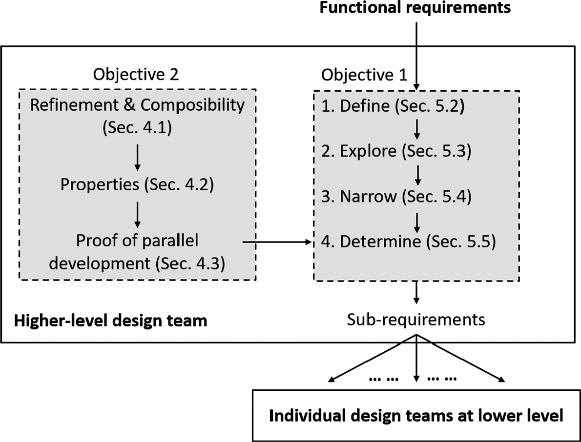
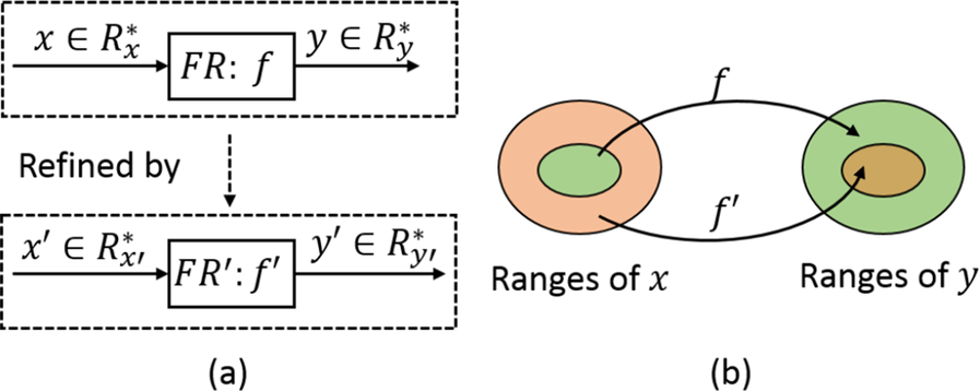





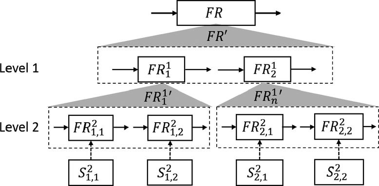
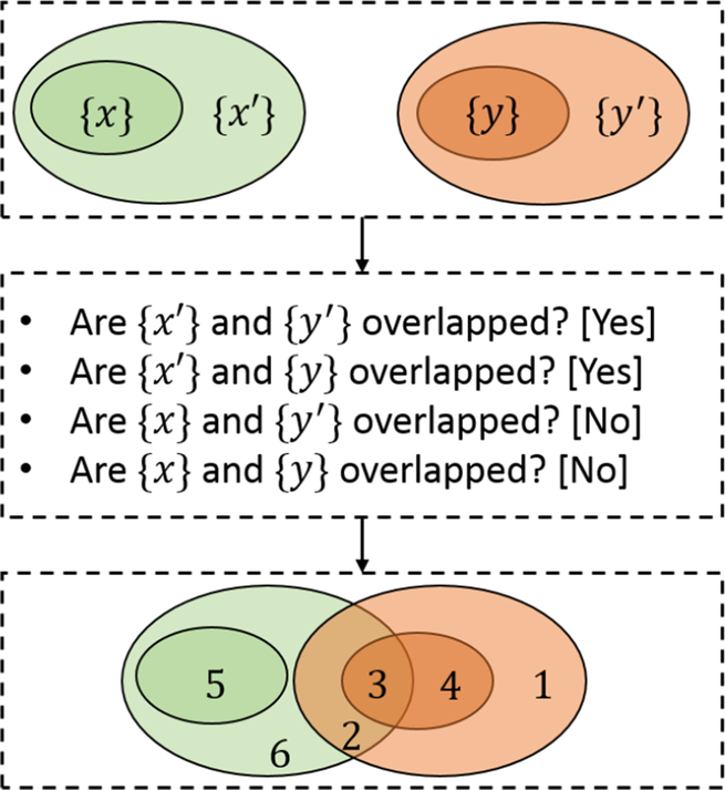


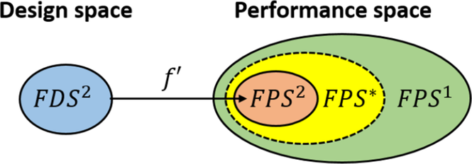

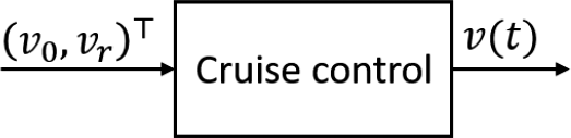
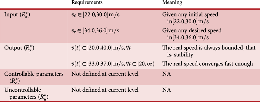
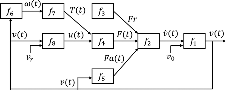
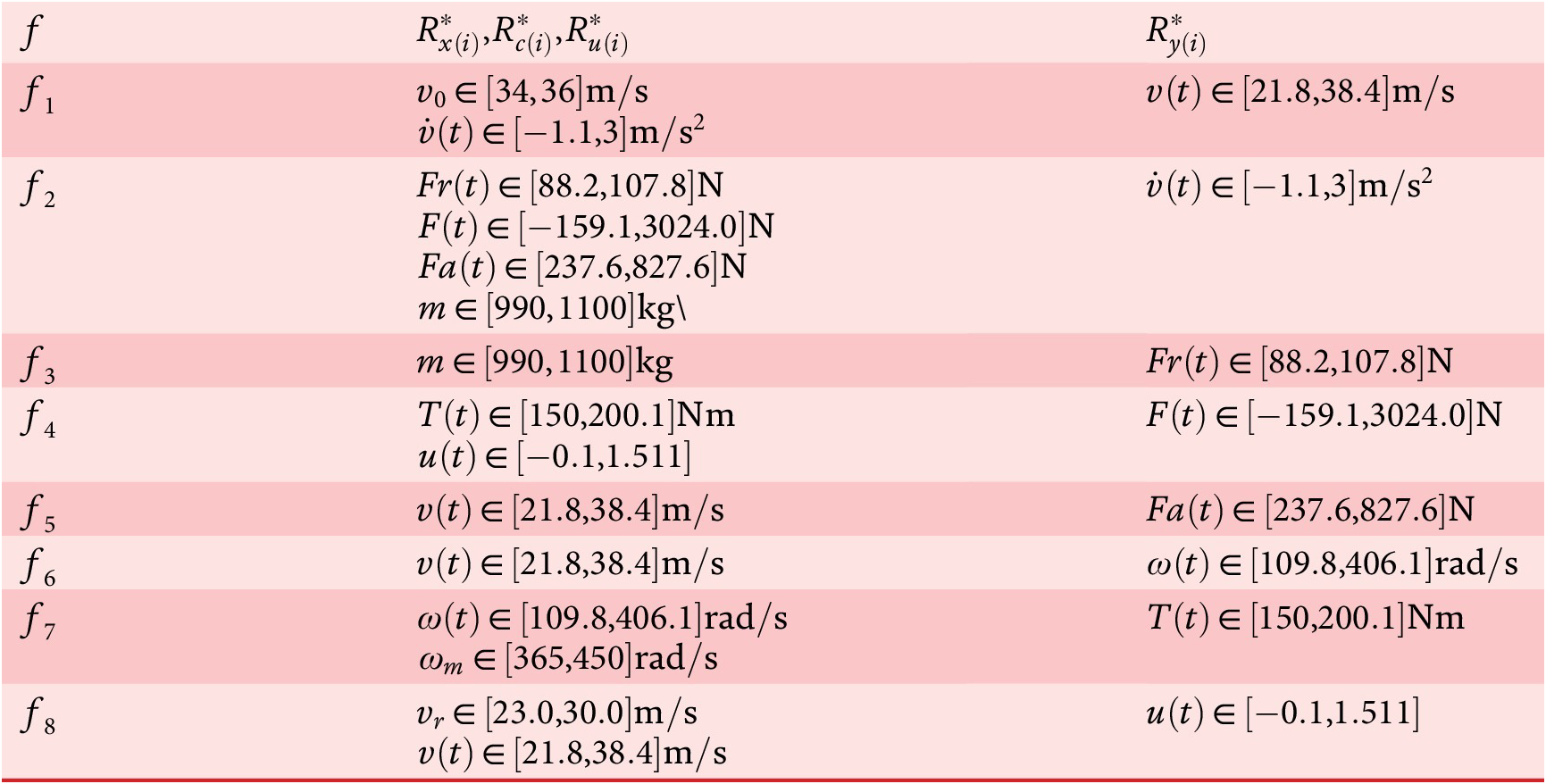
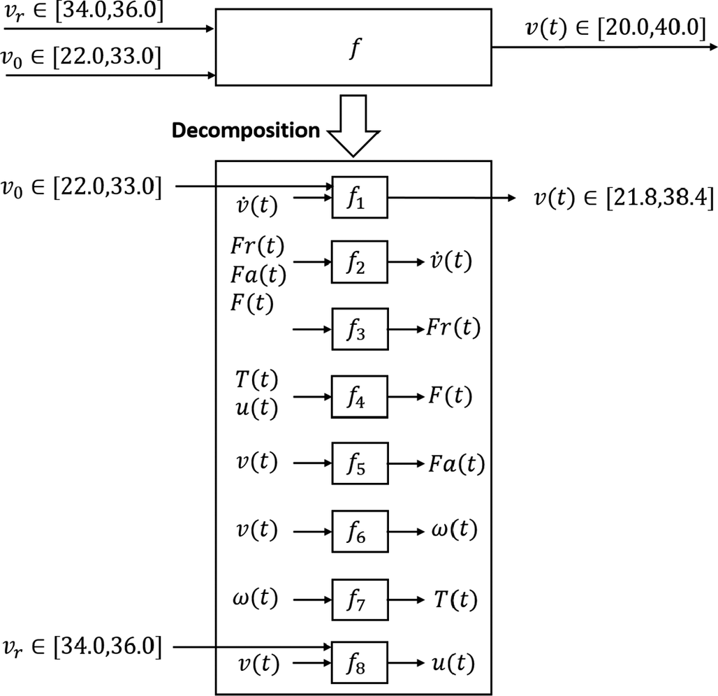

 Open access

