

1. Introduction
The purpose of this study is to investigate, using a numerical model, aspects of the melting and freezing processes that occur at an ice-shelf base. Melting occurs at an ice-shelf base because the sea water residing in the cavity beneath an ice shelf is relatively warm compared to the in situ pressure- depressed freezing point (Reference MilleroMillero, 1978); freezing occurs because warm waters in contact with the ice-shelf base undergo cooling and freshening and rise along the base, leading to the formation of frazil ice (Reference Lewis and PerkinLewis and Perkin, 1986). At the ice-shelf base, the net accumulation over time of this ice can produce a substantially thick layer of ice, commonly referred to as marine ice. This accumulated layer has been observed beneath all the major ice shelves of Antarctica, i.e. the Ronne Ice Shelf (Reference Thyssen, Bombosch and SandhägerThyssen and others, 1993; see their fig. 5), the Filchner Ice Shelf (Reference Grosfeld, Hellmer, Jonas, Sandhäger, Schulte, Vaughan, Jacobs and WeissGrosfeld and others, 1998; see their fig. 3) and the Amery Ice Shelf (Reference Fricker, Popov, Allison and YoungFricker and others, 2001; see their fig. 3b).
The thickness of the accumulated ice at an ice-shelf base is difficult to quantify, as direct observational evidence is lacking due to the logistical difficulty of accessing that remote surface. Some point measurements have been made by ice-core drilling from the surface down through to the base. For instance, on the Amery Ice Shelf a marine ice layer of approximately 150 m has been detected (Reference MorganMorgan, 1972), on the Ross Ice Shelf a 6 m layer (Reference Zotikov, Zagorodnov and RaikovskyZotikov and others, 1980), and on the Ronne Ice Shelf a layer of > 60 m (Reference OerterOerter and others, 1992). As compared to point measurements, a more spatially complete pattern of marine-ice thickness can be obtained by the use of airborne radio-echo sounding (Reference Robin, Doake, Kohnen, Crabtree, Jordan and MöllerRobin and others, 1983). As an example of this method, over the Ronne Ice Shelf a pattern of centralized accumulation of marine ice has been detected using this method (Reference Thyssen, Bombosch and SandhägerThyssen and others, 1993) that shows a maximum thickness of > 350 m. As another example, over the Amery Ice Shelf a pattern of thickness has been found, concentrated to the northwest, with a maximum thickness of 190 m (Reference Fricker, Popov, Allison and YoungFricker and others, 2001).
With an objective of estimating the contribution of basal thermodynamic processes to the overall mass balance of present-day ice shelves, some researchers have turned to numerical modeling. They have adopted the practice of using a fully three-dimensional, dynamical–thermodynamical ocean model but with a thermodynamical-only ice-shelf model (e.g. Reference Determann and GerdesDetermann and Gerdes, 1994; Reference Grosfeld, Gerdes and DetermannGrosfeld and others, 1997; Reference Williams, Warner and BuddWilliams and others, 1998; Reference Holland and JenkinsHolland and Jenkins, 2000). In such studies the ice-shelf “model” is in reality simply a parameterization of the fluxes of heat and fresh water that occur at the ice-shelf–ocean interface. The ice-shelf flow field does not play an explicit role in such a framework. Part of the justification for this approach lies with the significant disparity in time-scales between the slowly flowing ice shelf (e.g. 1 km a−1) and the relatively fast- flowing sub-ice-shelf waters (e.g. 10 cm s−1). Adopting this approach, one can simulate the spatial pattern of melting and freezing at an ice-shelf base. Such simulations are meaningful to the extent that a key assumption holds true: that the ice shelf is in a steady-state balance with respect to all possible sources and sinks of mass and heat.
The ability of a numerical model to simulate a marineice thickness layer, in rough accord with that directly observed, is useful because it lends greater confidence in the model-derived basal melting and freezing rates. Accurate knowledge of such rates is, after all, a critical component in making meaningful ice-shelf mass-balance estimates. The rates themselves are extremely difficult to derive by direct observational techniques. Some point measurements have been taken from holes opened at the ice-shelf base by hot-water drilling. An ultrasonic echo sounder has been deployed beneath one such hole in Ekströmisen and successfully used to directly record basal ablation (Reference Nixdorf, Oerter and MillerNixdorf and others, 1994). On the Filchner–Ronne, an alternative direct technique, based on electromagnetic measurements taken from transmission lines inserted into the melt hole, has been demonstrated capable of making relatively accurate measurements of basal ablation (Reference Grosfeld and BlindowGrosfeld and Blindow, 1993). The logistical support required for a single point measurement is significant and may thus preclude such direct techniques from providing us with spatial patterns of basal melting and freezing rates that span entire ice shelves.
Taking into consideration the above points, there is justification then in developing a numerical method for determining the present-day spatial pattern of thickness of the marine-ice layer beneath the major ice shelves of Antarctica. In this paper, we describe a numerical technique for calculating the thickness of the accreted marine-ice layer. The technique is based on mass conservation and is outlined in section 2. Some details about the existing ice-shelf and ocean models, which provide the necessary “forcing” data to the marine-ice thickness model, are given in section 3. An application of the modeling technique to an idealized ice-shelf–ocean geometry, illustrating the resulting steady-state pattern of marine-ice thickness, is presented in section 4. That section includes an analysis of the relative uncertainty in the computed thicknesses arising due to uncertainties in the forcing fields. The main conclusions of this work are drawn in section 5.
2. Marine Ice-Model
2.1. Thickness conservation equation
The idea of computing the thickness of the marine-ice layer, in a one-dimensional sense along a given horizontal flowline following the bottom of an ice shelf and based on the principle of conservation of mass, has been previously described (e.g. Reference Budd, Corry and JackaBudd and others, 1982), and applied to Antarctic ice shelves (e.g. Reference DetermannDetermann, 1991; Reference WilliamsWilliams, 1999). We now extend and generalize the one-dimensional horizontal description by carrying it over into a two-dimensional horizontal description in spherical coordinates as a step towards permitting present-day ice-shelf–ocean models to produce two-dimensional horizontal patterns of marine-ice thickness that can be compared with observed patterns. The goal is to compute the thickness of the marine-ice layer given complete knowledge of all other relevant features of the ice shelf, such as its total thickness, horizontal flow field and basal accumulation rate.
We simplify the treatment of the ice shelf by considering it to be vertically homogeneous such that the meteoric and marine-ice components have the same density. The statement of mass conservation under conditions of incompressible flow becomes equivalent to the statement of volume conservation. The volume balance equation for a given vertical column of ice shelf is then derived by treating the ice surface and base as material surfaces upon which ice-volume sources and sinks act. At the ice-shelf surface z
s meteoric ice accumulates at a rate
![]() and thus the position of the ice-shelf surface is the kinematic boundary condition
and thus the position of the ice-shelf surface is the kinematic boundary condition
where w s is the vertical velocity at the surface. In this context, the material derivative assumes the two-dimensional form

The last relation is strictly valid only for flat geometries, but the approximation is well justified by the fact that the neglected curvature terms are very small in the present application because of the relatively small horizontal scale of an ice shelf as compared to the scale of the Earth. The components of the depth-independent ice-shelf horizontal flow velocity are defined as U
i and V
i, or equivalently expressed in vector form as
![]() (see Fig. 1). Throughout this paper the independent variables x, y, z and t have their usual meanings. Analogous to the surface, the position of the ice-shelf base z
b, changes as it accumulates marine ice at a rate
(see Fig. 1). Throughout this paper the independent variables x, y, z and t have their usual meanings. Analogous to the surface, the position of the ice-shelf base z
b, changes as it accumulates marine ice at a rate
![]() so that the kinematic boundary condition is
so that the kinematic boundary condition is
where w b is the vertical velocity at the base. The total thickness of the ice shelf is defined as the difference H i = z s − z b. Vertically integrating the incompressibility condition for the three-dimensional flow of the ice shelf, assuming no vertical shear in the horizontal flow field, applying the boundary conditions of Equations (1) and (3), then a conservation equation for the total ice-shelf thickness is derived as
A vertical slice in the yz-coordinate plane showing the ice shelf, the ocean waters in the sub-ice-shelf cavity, and the underlying bedrock. The ice shelf is of a total thickness H
i
which includes both the meteoric and marine-ice contributions. The surface of the ice shelf is located at z
s
, and the base at z
b
. The respective accumulation rates of snow and ice at the surface and the bottom are
![]() and
and
![]() , respectively (both taken at the ice- equivalent density) where the overlying dot notation represents a time derivative. The marine-ice thickness component of the total thickness is h
m
and is shown as the darker, shaded patches. The vertically uniform flow of the ice shelf is
, respectively (both taken at the ice- equivalent density) where the overlying dot notation represents a time derivative. The marine-ice thickness component of the total thickness is h
m
and is shown as the darker, shaded patches. The vertically uniform flow of the ice shelf is
![]() while the vertically non-uniform flow of the ocean waters is
while the vertically non-uniform flow of the ocean waters is
![]() .
.
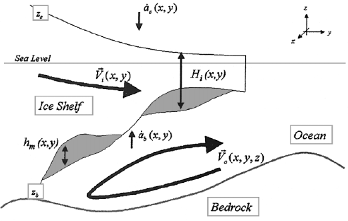
The internal interface between the meteoric and marine ice is taken to be a material surface since we do not allow any transformational processes, such as molecular diffusion, to operate at that interface. This means that we can write separate relations, based on Equation (4), for the meteoric h a and marine h m layers as
Built into this model is the reasonable assumption that the flow velocity of the meteoric and marine-ice layers is identical, or equivalently that there is no vertical shear in the horizontal ice-flow field (Reference Sanderson and DoakeSanderson and Doake, 1979). To solve Equation (6), and thus obtain the thickness of the marine-ice layer, we need to know the ice-shelf velocity field
![]() and the basal accumulation rate
and the basal accumulation rate
![]() . Later on, we provide estimates for these, with the ice-shelf velocity field being obtained from a solution of the ice-shelf flow evolution equation (section 3.2) and the basal accumulation rate derived from a three-layer formulation of heat and fresh-water exchange between the ice-shelf base and the ocean waters in the sub-ice-shelf cavity (section 3.3). For the moment, we assume these quantities as known. We also later examine the sensitivity of the simulated marine-ice thickness to uncertainty in the magnitude of these “forcing”quantities (section 4.2).
. Later on, we provide estimates for these, with the ice-shelf velocity field being obtained from a solution of the ice-shelf flow evolution equation (section 3.2) and the basal accumulation rate derived from a three-layer formulation of heat and fresh-water exchange between the ice-shelf base and the ocean waters in the sub-ice-shelf cavity (section 3.3). For the moment, we assume these quantities as known. We also later examine the sensitivity of the simulated marine-ice thickness to uncertainty in the magnitude of these “forcing”quantities (section 4.2).
2.2. Numerical solution technique
We describe an accurate, efficient algorithm to numerically solve Equation (6). We first introduce subscripts which refer to a grid index, namely, i and j referring to lattice positions in the
![]() and
and
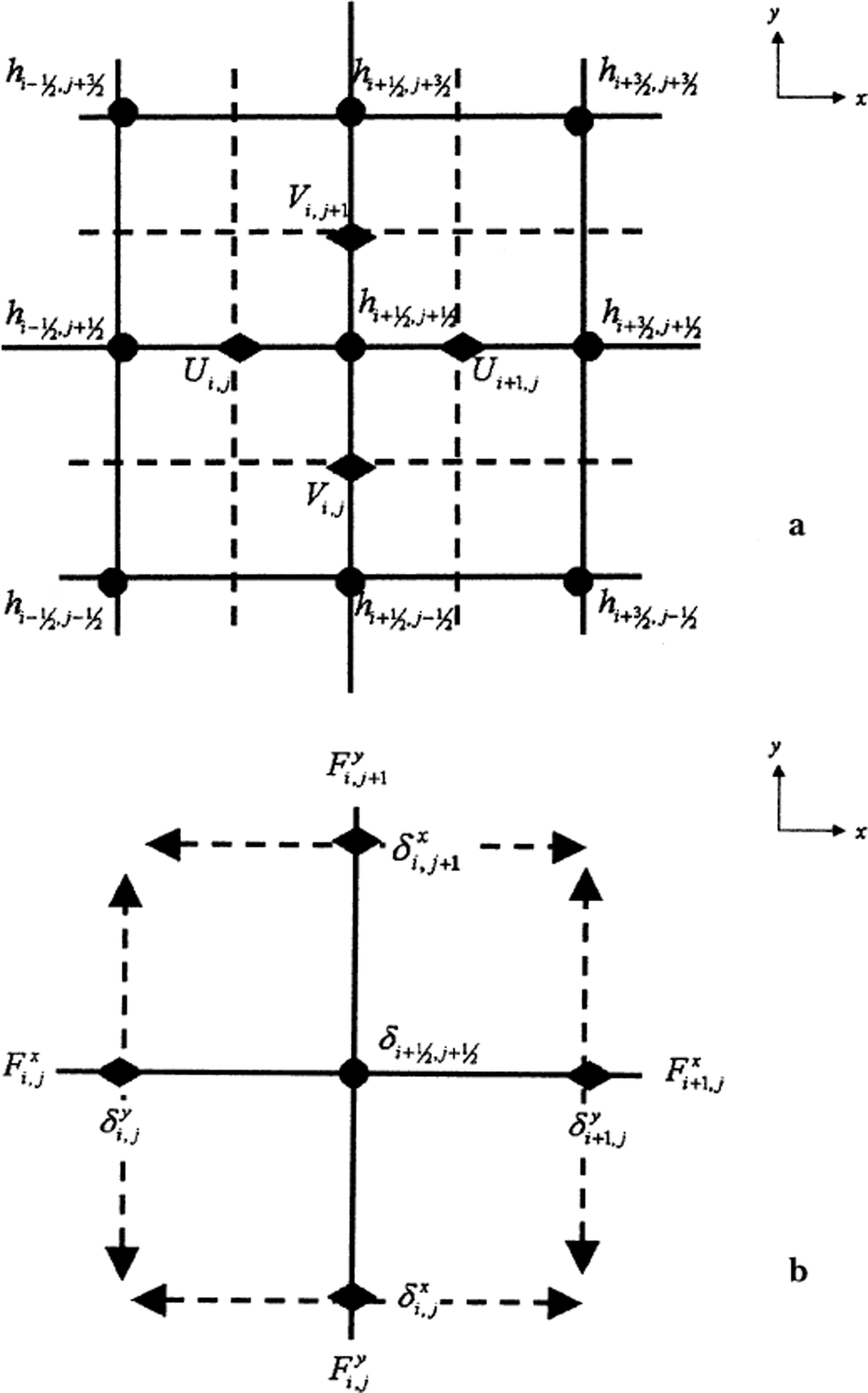
![]() coordinate directions, respectively, and a superscript t which refers to time index, or equivalently, an iteration index. The discretization of the volume-conservation relation, Equation (6), is carried out on a C-grid stencil (Reference Arakawa and LambArakawa and Lamb, 1977; see Fig. 2a).
coordinate directions, respectively, and a superscript t which refers to time index, or equivalently, an iteration index. The discretization of the volume-conservation relation, Equation (6), is carried out on a C-grid stencil (Reference Arakawa and LambArakawa and Lamb, 1977; see Fig. 2a).
Grid stencil for discretization of the marine-ice thickness layer evolution equation. (a) The stencil has scalar quantities, i. e. the marine-ice thickness
![]() defined by the solid-circle symbols and referred to as the scalar gridpoints, occurring at the intersection of the solid lines. The vector components, i.e. the ice- flow field U
i,j
and V
i,j
, defined by the solid-diamond symbols and referred to as the vector gridpoints, occur at the intersection of a solid and a dashed line. This arrangement is known as the C-grid stencil (Reference Arakawa and LambArakawa and Lamb, 1977). The grid indices are denoted by subscripts i and j in the
defined by the solid-circle symbols and referred to as the scalar gridpoints, occurring at the intersection of the solid lines. The vector components, i.e. the ice- flow field U
i,j
and V
i,j
, defined by the solid-diamond symbols and referred to as the vector gridpoints, occur at the intersection of a solid and a dashed line. This arrangement is known as the C-grid stencil (Reference Arakawa and LambArakawa and Lamb, 1977). The grid indices are denoted by subscripts i and j in the
![]() and
and
![]() directions, respectively, where full-integer indices occur at the vector gridpoints and half-integers occur at the scalar gridpoints. (b) Stencil definitions for auxiliary variables used in the flux divergence calculation.
directions, respectively, where full-integer indices occur at the vector gridpoints and half-integers occur at the scalar gridpoints. (b) Stencil definitions for auxiliary variables used in the flux divergence calculation.
![]() and
and
![]() are the zonal and meridional volume fluxes and are defined at the vector gridpoints. The grid spacing in the zonal and meridional directions is defined by the “distance” functions and
are the zonal and meridional volume fluxes and are defined at the vector gridpoints. The grid spacing in the zonal and meridional directions is defined by the “distance” functions and
![]() and
and
![]() , respectively, defined at the vector gridpoints. The grid spacing at scalar gridpoints, represented by
, respectively, defined at the vector gridpoints. The grid spacing at scalar gridpoints, represented by
![]() , is obtained by averaging neighboring grid spacings as defined at vector points.
, is obtained by averaging neighboring grid spacings as defined at vector points.
We represent the divergence operator of Equation (6) in spherical coordinates and we temporarily utilize the Earth’s spherical coordinate notation with λ being the longitude and φ the latitude coordinate, both expressed in degree angle measure. The flux-divergence term in the volumeconservation relation, Equation (6), can be expressed in terms of a volume-flux vector
![]() in a (λ, φ) spherical-coordinate system as
in a (λ, φ) spherical-coordinate system as
with
![]() and
and
![]() being the unit vectors in the longitudinal and latitudinal directions, respectively, and F
λ
and F
φ
the respective volume fluxes. We can then rewrite this expression in terms of a coordinate system defined with the independent variables (x, y) defined according to
being the unit vectors in the longitudinal and latitudinal directions, respectively, and F
λ
and F
φ
the respective volume fluxes. We can then rewrite this expression in terms of a coordinate system defined with the independent variables (x, y) defined according to
where the differential relations between the two coordinate systems are
and the first differential relation makes additional use of the fact that φ is independent of x. We introduce a “distance” function δ defined as
where δλ , φ is a constant.
The use of a C-grid stencil means that the lateral volume fluxes will be defined at the vector gridpoints, while the flux divergence
![]() will be defined at the scalar, or marine-ice thickness, gridpoints (see Fig. 2b). Using a first-order accurate Taylor series expansion of the volume-flux vector
will be defined at the scalar, or marine-ice thickness, gridpoints (see Fig. 2b). Using a first-order accurate Taylor series expansion of the volume-flux vector
![]() leads to the finite-difference expression of the flux divergence as
leads to the finite-difference expression of the flux divergence as

This expression fully retains the spherical-coordinate attributes of the underlying grid.
A potential mechanism leading to undesirable negative marine-ice thickness may occur when the forcing term
![]() goes negative, i.e. during basal melting events. When this term is negative, and there is no marine ice present, we suppress it. Consequently, we insist that the actual source–sink term for the marine ice is expressed in terms of a related quantity
goes negative, i.e. during basal melting events. When this term is negative, and there is no marine ice present, we suppress it. Consequently, we insist that the actual source–sink term for the marine ice is expressed in terms of a related quantity
![]() , later referred to as the “corrected” accumulation rate, as
, later referred to as the “corrected” accumulation rate, as

where H[·] represents the Heaviside step function and ε is a small positive quantity.
Using the spatial discretization of Equation (11) we carry out an iterative solution to the marine-ice thickness relation, Equation (6), by discretizing it in time as

where δt is the effective “time-step” of the iteration procedure as it marches towards a steady-state solution. This is a relaxation procedure whereby we terminate the algorithm upon minimizing sequential differences in the L 1 norm of the marine-ice thickness according to the measure
where the tolerance is specified as a small fraction normalized by the number of gridpoints as ε
tol = [10−4 · NxNy
]. In the last expression, Nx
and Ny
are the number of gridpoints in the
![]() and
and
![]() directions, respectively.
directions, respectively.
An appropriate value for the “time-step” increment δt can be derived with a physical argument based on the travel time for an average particle to traverse the entire ice shelf by entering at the grounding line and leaving at the ice-shelf front. For a typical ice shelf of dimension L = 500 km and travel velocity U = 0.5 km a−1 the total traversal time would be of order T = L/U ≈ 103 years. This is a rough estimate of the time for the marine-ice thickness to establish an equilibrium pattern, and so a reasonable δt is a small fraction of this. In practice, therefore, we take δt = 1 year and iterate for a maximum total length of time T = 103 years, unless the condition of Equation (14) is met first, in which case the algorithm terminates. It is also noted that this particular integration period and time-step apply only to the solution of the marine-ice thickness layer equation and not to the ocean model, which is later introduced.
In Figure 3 we illustrate a plan view of the ice shelf, the key model variables and also the treatment of the lateral boundary conditions. A further discussion of the detailed aspects of the numerical procedure (e.g. the design and application of the lateral boundary conditions as depicted in Figure 3) may be found elsewhere (http://fish.cims.nyu.edu/project_oisi/marine_ice_thickness/j_glac_supplement.html).
Plan view in the xy-plane of an ice shelf surrounded by a continental ice sheet and open ocean. The heavy black lines show the ice flow
![]() originating from the ice sheet, traversing the grounding line (dotted line), flowing across the ice shelf, and ultimately reaching the ice-shelf front (dashed line). The darker, shaded patches show a marine-ice layer h
m
(x, y) embedded at the underside of the ice shelf of thickness H
i
(x,y). The ice shelf is delimited by the horizontal domain Ω and enclosed by the lateral boundary ∂Ω. The boundary conditions applied along the lateral boundary ∂Ω are of zero marine-ice thickness h
m
= 0 along the grounding line and zero normal gradients ∂h
m
/∂n along the remaining boundaries (where
originating from the ice sheet, traversing the grounding line (dotted line), flowing across the ice shelf, and ultimately reaching the ice-shelf front (dashed line). The darker, shaded patches show a marine-ice layer h
m
(x, y) embedded at the underside of the ice shelf of thickness H
i
(x,y). The ice shelf is delimited by the horizontal domain Ω and enclosed by the lateral boundary ∂Ω. The boundary conditions applied along the lateral boundary ∂Ω are of zero marine-ice thickness h
m
= 0 along the grounding line and zero normal gradients ∂h
m
/∂n along the remaining boundaries (where
![]() denotes the outward normal direction).
denotes the outward normal direction).

3. Supporting Models
The marine-ice thickness model requires knowledge of various ice-shelf and ocean “forcing” fields, most notably the ice- shelf thickness, ice-shelf velocity and ice-shelf basal accumulation rate. The evaluation of the latter field can be achieved via the use of a three-dimensional ocean-general-circulation model, a brief description of which is provided at the end of this section. The development of that ocean model has occurred within the framework of a longer-term modeling effort, referred to as the Polar Ocean Land Atmosphere Ice Regional (POLAIR) modeling system, which is focused on investigating various aspects of ice–ocean interaction, the phenomena of marine-ice layers being one such aspect. We now describe the “supporting” models that yield the information necessary to compute marine-ice thickness patterns according to the discretized relation of Equation (13).
3.1. Ice-shelf thickness
A prognostic equation describing the evolution of the ice- shelf thickness, as derived from the standard fluid dynamical assumptions of mass conservation and incompressibility, was given as Equation (4). In the steady-state context of the present study we will not be evolving the ice-shelf thickness, but rather will be taking it as a specified, constant field throughout the model integration. Part of the motivation for this approach is that in the situation whereby one would like to determine the marine-ice thickness pattern of a real Antarctic ice shelf, one would start by using as input data the present-day observed thickness pattern of the ice shelf. This pattern, whether derived from radio sounding estimates or satellite altimeter measurements, would of necessity include both the meteoric and marine-ice components, thus giving a “total” ice-shelf thickness field H i. Since the marine-ice thickness field h m is already included within such a total ice-shelf thickness field H i, and since we are interested in determining the present-day pattern of marine-ice thickness, we will then not evolve the total ice-shelf thickness pattern.
The idealized ice shelf we are using takes the shape of a “sector” in spherical coordinates. It is oriented in the meridional direction, with lines of constant longitude forming the sidewalls. The grounding line is located at the southern extreme of the sector along a line of constant latitude, and the ice front is located along a more northerly line of constant latitude. There are no longitudinal thickness variations. The complete, idealized model domain as sketched in Figure 4 shows the ice shelf being fully contained within a larger oceanic domain. We refer to that part of the ocean domain not covered by the ice shelf as the open-ocean domain, and to the complementary part as the sub-ice-shelf domain. The entire domain is horizontally discretized with a grid spacing of δλφ = 1.0° angular measure. At the grounding line this equates to a grid spacing of about 10 km.
Plan view of model domain for idealized ice-shelf calculations in a spherical-coordinate system. The ocean domain extends south–north from 85° S to 75° S and west–east from 10° W to 10° E. The ice-shelf domain, shown as the stippled area, exists only in the southern part of the ocean domain. The grounding line occurs at the latitude line 85° S (dotted line) across which flows a specified ice volume flux of 20 km3a−1. The ice-shelf front occurs across the latitude line 80° S (dashed line). The ice shelf is bounded to the west and east by sidewalls through which no volume flux may occur.

Given an idealized ice shelf having spatial extent as outlined, we need to create a meaningful total thickness pattern. This can be achieved by following along an approximated theory that states that the thickness gradient of an ice shelf is independent of accumulation rates, ice-shelf thickness and ice-shelf velocity fields (Reference SandersonSanderson, 1979). The meridional thickness gradient ∂H i(y)/∂y for a meridionally oriented idealized ice shelf is then approximated as

where the constant τ 0 is a stress-related parameter, taken to be 90 kPa, W(y) is the meridionally dependent width of the ice shelf, g is the acceleration due to gravity taken as 9.81 m s−2, ρ i is the ice-shelf density in kg m−3, and ρ o is a mean ocean water density of 1025.0 kg m−3. Equation (15) states that the thickness gradient is inversely proportional to the width of the ice shelf, a feature confirmed by field data (Reference SandersonSanderson, 1979). Although the sidewalls of the ice shelf are lines of constant longitude, the ice shelf does actually widen as one traverses it in a northerly direction because of the use of a spherical-coordinate system. The width W(y) of the idealized ice shelf is a function then of only the meridional coordinate y.
It should be noted that Equation (15) was originally derived in the context of a constant-width domain, and the validity of its application in the present context of a varying- width domain has not been proven. However, as Equation (15) is used simply for the purpose of creating an idealized ice-shelf thickness pattern, we overlook this point in the present idealized application.
The ice-shelf thickness is evaluated starting at the ice- shelf front y f, where the ice-shelf thickness is specified as a constant of integration, and then integrating Equation (15) southward to a latitude line y, so

The numerical integration of Equation (16) on a spherical- coordinate grid is a straightforward task. It conveniently gives a discrete, constant ice-shelf profile to use in the computation of the marine-ice thickness field. Setting the ice-shelf front thickness H(y f) to be 100 m, we arrive at the ice-shelf profile depicted in Figure 5a where the thickness at the grounding line H(y g) has reached a value of just over 800 m.
North–south transect of the idealized ice-shelf properties: (a) thickness H i in units of m, (b) density in units ρ i of kg m−3, and (c) surface elevation z s in units of m.
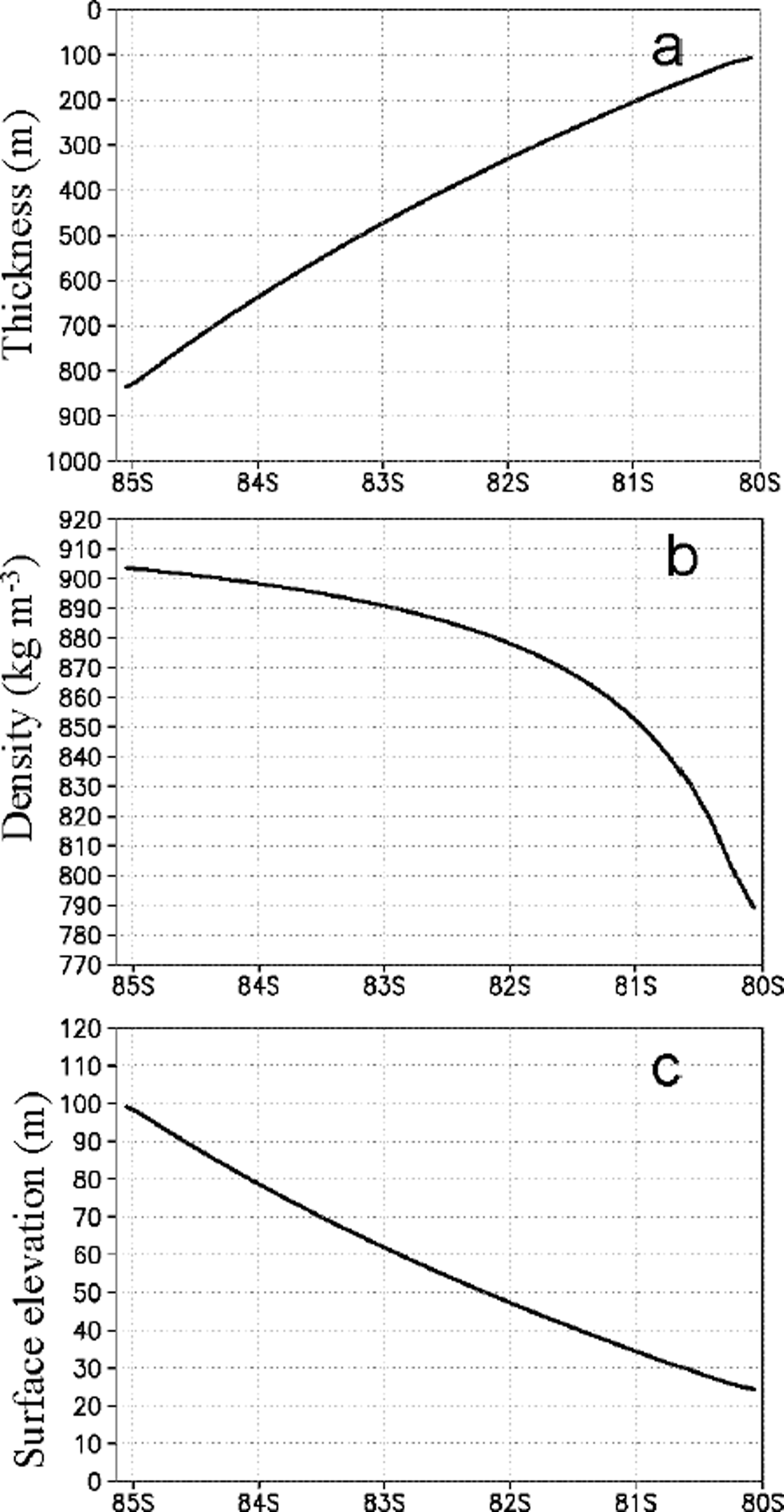
Knowing the ice-shelf thickness, there are two additional quantities that we can now derive, namely, the ice-shelf density and surface elevation (Reference ThyssenThyssen, 1988). The spatially dependent density is a consequence of assuming a constant-thickness firn layer residing near the ice-shelf surface. A well- known empirical relation (Reference ThyssenThyssen, 1988) is

where at present the ice-shelf thickness H i(y) derives from Equation (16). The density ρ i(y) in the above expression has units of kg m−3 when the thickness H i(y) is expressed in m. The computed density is shown in Figure 5b. Knowing the ice-shelf density ρ i(y), we can then compute the ice-shelf surface elevation z s(y) from Archimedes’ principle as

where knowledge of the density ρ i(y) comes from Equation (17) and the thickness H i(y) from Equation (16). The computed surface elevation is shown in Figure 5c.
3.2. Ice-shelf velocity
3.2.1. Governing equations
For a unit volume of ice shelf, the basic differential equation describing the flow field follows from the statement that the divergence of the three-dimensional stress tensor exactly equals the only external force operating on the system, namely, that of gravity, and so
where
![]() is the three-dimensional stress tensor, having components denoted τij
, and
is the three-dimensional stress tensor, having components denoted τij
, and
![]() is the gravitational acceleration vector. The ij subscripts are meant to indicate permutations of the x,y and z coordinate directions. Instead of using components of the stress tensor, this relation can be converted into one involving the three-dimensional strain-rate tensor
is the gravitational acceleration vector. The ij subscripts are meant to indicate permutations of the x,y and z coordinate directions. Instead of using components of the stress tensor, this relation can be converted into one involving the three-dimensional strain-rate tensor
![]() , having components denoted
, having components denoted
![]() , by introducing a flow law (Glen, 1955)
, by introducing a flow law (Glen, 1955)
where A is a temperature-dependent ice-stiffness parameter having a value of approximately 2.0 × 10⁻²⁵ Pa−3 s−1, which corresponds to ice at a temperature of about −20°C. In Equation (20) we have also introduced τ, the effective deviator stress, and
![]() , the components of the stress deviator (see Reference PatersonPaterson, 1994, for further details). The flow-law exponent N is generally taken to be equal to three. Employing the usual relation between strain rates and velocity gradients
, the components of the stress deviator (see Reference PatersonPaterson, 1994, for further details). The flow-law exponent N is generally taken to be equal to three. Employing the usual relation between strain rates and velocity gradients

we can then transform Equation (19) from one based on strains to one involving only velocity gradients. The resulting two-dimensional horizontal-flow equations, after several simplifying assumptions (Reference Morland, Van der Veen and OerlemansMorland, 1987), become

The depth-averaged effective viscosity
![]() is defined as
is defined as

in which the vertical integration is taken from the ice-shelf base located at z
b to the surface at z
s. The effective viscosity is inversely proportional to the flow strain rates, and so the flow behavior is such that the ice “fluid” becomes less viscous the more the flow field develops divergent and shear strains. In the present study we ignore all terms involving the spatial gradients of
![]() occurring in Equation (22), a simplification adopted in previous ice-shelf flow modeling (e.g. Reference DetermannDetermann, 1991).
occurring in Equation (22), a simplification adopted in previous ice-shelf flow modeling (e.g. Reference DetermannDetermann, 1991).
3.2.2. Boundary conditions
Along the perimeter of the ice shelf, three different types of boundary conditions are applied, depending on the exact nature of the boundary. Along sections of the grounding line where ice streams enter into the ice shelf we specify the volume flux Ψi|
∂
Ω of the ice stream. Given that we know the thickness H
i|
∂
Ω of the ice shelf at such locations, we can convert the volume flux to a two-dimensional horizontal flow vector
![]() that serves directly as a Dirichlet-type boundary condition on the flow Equations (22). In the instance that a simulation involved a real Antarctic ice shelf, such fluxes would come from estimates based on field or satellite observations. In our idealized study, we specify a volume flux of Ψi|
∂
Ω = 20 km3 a−1 along the entire southern grounding line, a line of constant latitude. That flux is equivalent to a flow velocity of about 0.05 km a−1, given the assigned thickness and width of the ice shelf along the grounding line. Along sections of the grounding line where there are no ice streams, we specify the volume flux as zero, Ψi|
∂
Ω = 0. In our idealized ice-shelf configuration this is equivalent to stating that the sidewalls of the ice shelf, which are lines of constant longitude, have no ice-volume sources or sinks.
that serves directly as a Dirichlet-type boundary condition on the flow Equations (22). In the instance that a simulation involved a real Antarctic ice shelf, such fluxes would come from estimates based on field or satellite observations. In our idealized study, we specify a volume flux of Ψi|
∂
Ω = 20 km3 a−1 along the entire southern grounding line, a line of constant latitude. That flux is equivalent to a flow velocity of about 0.05 km a−1, given the assigned thickness and width of the ice shelf along the grounding line. Along sections of the grounding line where there are no ice streams, we specify the volume flux as zero, Ψi|
∂
Ω = 0. In our idealized ice-shelf configuration this is equivalent to stating that the sidewalls of the ice shelf, which are lines of constant longitude, have no ice-volume sources or sinks.
The treatment of boundary conditions along the ice-shelf front is more complicated, partly because shear stresses are introduced in the yz-plane by the unbalanced hydrostatic pressure along the ice “cliff”. Nonetheless, an approximated expression for the strain rate for an ice shelf spreading in one dimension (Reference ThomasThomas, 1973) in the form of a Neumann-type boundary condition is

where n denotes the coordinate direction normal to the ice- shelf front. In our idealized ice-shelf set-up, the ice front is taken as a line of constant latitude, and so in Equation (24) we could in fact replace n directly by y.
3.2.3. Numerical solution technique
Equations (22–24) governing the flow, the viscosity and the boundary conditions, respectively, are discretized on a spherical-coordinate C-grid in much the same manner as that outlined in section 2 for the marine-ice layer equation. The use of a spherical coordinate system is fully accounted for in the discretization process by making all gridcells “locally” square exactly as for the marine-ice thickness equation. The solution technique is that of successive overrelaxation (with an overrelaxation parameter of 1.2). The domain grid is separated into a checkerboard-like grid yielding two “sub-grids”, which we refer to as the “white” and “black” grids. On alternating iterations the white gridcells are updated using data from the black gridcells, and vice versa on the succeeding iteration. Such a checkerboard scheme is amenable to automatic code parallelization as it only uses gridcell data from nearest neighbors and thus renders the solution technique efficient on modern, parallel-computing platforms (Reference Press, Teukolsky, Vetterling and FlanneryPress and others, 1996) such as a multi-processor Cray J90 as used in this study. Testing of the model showed that convergence, defined in terms of the behavior of the L 1 norm of the ice-shelf kinetic energy, reached 0.1% of its asymptotic value after less than 2000 iterations. The equilibrium flow field resulting from the iteration procedure is shown in Figure 6.
Two-dimensional horizontal ice-shelf flow field
![]() . The flow intensity is given by the color bar to the right and has units of km a−1. The equilibrium flow field, after approximately 2000 iterations, shows a peak flow of about 0.75 km a−1 occurring near the middle of the ice-shelf front, away from the retarding influence of the sidewalls. Note that only the ice-shelf-covered portion of the total domain is shown. Incidentally, the initial flow field is everywhere zero except for the specified velocity along the grounding line where the velocity is approximately 0. 05 km a−1.
. The flow intensity is given by the color bar to the right and has units of km a−1. The equilibrium flow field, after approximately 2000 iterations, shows a peak flow of about 0.75 km a−1 occurring near the middle of the ice-shelf front, away from the retarding influence of the sidewalls. Note that only the ice-shelf-covered portion of the total domain is shown. Incidentally, the initial flow field is everywhere zero except for the specified velocity along the grounding line where the velocity is approximately 0. 05 km a−1.

3.3. Basal accumulation
The procedure outlined in section 2 for estimating the marine-ice thickness is sensitive to the degree of realism with which the basal accumulation and ablation rates can be modeled. To make computation of such rates as accurate as possible, it is necessary to determine the physical characteristics exactly at the ice-shelf–ocean interface where there are three physical constraints: the interface must be at the freezing point and both heat and salt must be conserved at the interface during any phase changes. This description can be configured to give a system of three linear equations in three unknowns, namely, the interface temperature T
b, salinity S
b and the ice-shelf basal accumulation rate
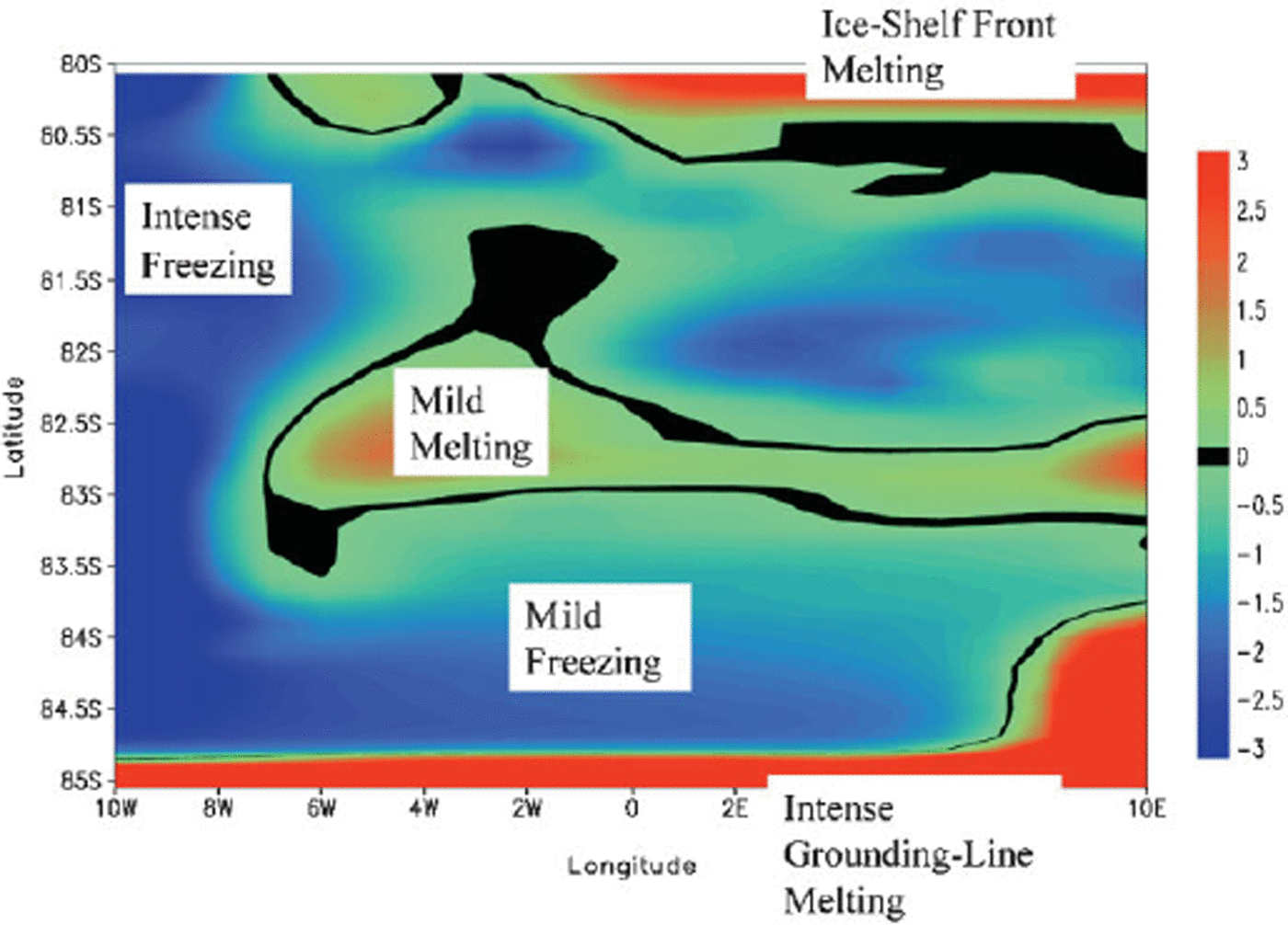
![]() , all of which may be solved for simultaneously. Such an approach is commonly referred to as a “viscous-sublayer”“ parameterization of thermodynamic exchange, because the actual fluxes of heat and salt are modeled to occur by molecular diffusion in a thin viscous fluid layer attached to the ice-shelf–ocean interface. Details on the exact formulation of this modeling approach are outlined elsewhere (Reference Holland and JenkinsHolland and Jenkins, 1999). The simulated melt rate at the ice-shelf base arising from application of the viscous-sublayer model is shown in Figure 7.
, all of which may be solved for simultaneously. Such an approach is commonly referred to as a “viscous-sublayer”“ parameterization of thermodynamic exchange, because the actual fluxes of heat and salt are modeled to occur by molecular diffusion in a thin viscous fluid layer attached to the ice-shelf–ocean interface. Details on the exact formulation of this modeling approach are outlined elsewhere (Reference Holland and JenkinsHolland and Jenkins, 1999). The simulated melt rate at the ice-shelf base arising from application of the viscous-sublayer model is shown in Figure 7.
Pattern of ice-shelf basal melting (red zones) and freezing (blue zones) from the model simulation. The black zones correspond to areas where ice is neither melting nor freezing. The contour range is taken between ±3 cm a−1 to optimize the visual impression between the melting and freezing zones. The actual maximum melting rate is well above the contoured range, and has an intensity of about 80 cm a−1 that occurs in the southeastern corner The actual maximum basal freezing rate is below the contoured range, and has an intensity of about −8 cm a−1 that occurs in the northwestern part of the domain. Overall, melting dominates freezing, and averaged over the entire ice-shelf base, there is a net melting of 0.5 cm a−1.
3.4. Ocean model
The fully prognostic, three-dimensional circulation field
![]() of the ocean waters in the sub-ice-shelf cavity (see Fig. 1) is modeled using an isopycnic-coordinate, ocean-general-circulation model (Reference Bleck, Rooth, Hu and SmithBleck and others, 1992) which includes an embedded mixed-layer turbulent-kinetic-energy parameterization (Reference GasparGaspar, 1988) in its uppermost layer. The ocean model has been reformulated so as to be able to deal with the inclusion of arbitrary bottom and surface topographies, and as such is well suited to the problem of ice-shelf-ocean interaction (Reference Holland and JenkinsHolland and Jenkins, 2000). The model has been designed such that the interconnection between the open-ocean part of the domain and the sub-ice-shelf part is seamless; there is no requirement for application of any sort of artificial boundary condition to join these two subdomains. The only boundary conditions applied to the ocean model are that of no normal fluid flow through any of its boundaries and that of no heat or salt flow through any boundaries, except the thermodynamic exchange occurring at the ice-shelf base as described in section 3.3. Geothermal heat fluxes through the sea floor are not considered. Over the open-ocean part of the domain, surface stress and buoyancy fluxes can be included but are presently set to zero for the purposes of this idealized study.
of the ocean waters in the sub-ice-shelf cavity (see Fig. 1) is modeled using an isopycnic-coordinate, ocean-general-circulation model (Reference Bleck, Rooth, Hu and SmithBleck and others, 1992) which includes an embedded mixed-layer turbulent-kinetic-energy parameterization (Reference GasparGaspar, 1988) in its uppermost layer. The ocean model has been reformulated so as to be able to deal with the inclusion of arbitrary bottom and surface topographies, and as such is well suited to the problem of ice-shelf-ocean interaction (Reference Holland and JenkinsHolland and Jenkins, 2000). The model has been designed such that the interconnection between the open-ocean part of the domain and the sub-ice-shelf part is seamless; there is no requirement for application of any sort of artificial boundary condition to join these two subdomains. The only boundary conditions applied to the ocean model are that of no normal fluid flow through any of its boundaries and that of no heat or salt flow through any boundaries, except the thermodynamic exchange occurring at the ice-shelf base as described in section 3.3. Geothermal heat fluxes through the sea floor are not considered. Over the open-ocean part of the domain, surface stress and buoyancy fluxes can be included but are presently set to zero for the purposes of this idealized study.
The ocean model produces an “ice-pump”-type circulation as principally forced by the pressure-dependent freezing point of sea water (Reference Lewis and PerkinLewis and Perkin, 1986). This circulation is created by the melting and freezing patterns at the ice-shelf base, and, in turn, this circulation fundamentally modifies the intensity of those thermodynamical processes that created it in the first place. From the point of view of the present study, the ocean model is of relevance in that it produces the “forcing” pattern of corrected accumulation
![]() that acts as the source term for marine-ice growth. It does this by prognostically computing the ocean mixed-layer temperatures T
m, salinities S
m and flow field
that acts as the source term for marine-ice growth. It does this by prognostically computing the ocean mixed-layer temperatures T
m, salinities S
m and flow field
![]() .
.
The ocean domain is set to everywhere have a flat-bottom topography of depth 1000 m. The ocean model horizontal grid exactly mimics all other grids used in the study. The ice shelf of thickness depicted in Figure 5a floats upon the ocean surface in the southern part of the ocean domain, thus giving the ocean a surface topography in that region. The ocean is assigned to have ten equal-thickness isopycnic layers, initially all set to have a temperature of −1.8°C, and to be uniformly stratified in salinity over the range 34.4–34.8 psu (practical salinity units). The initial conditions are designed to represent the typical range of water-mass properties commonly found along the Antarctic continental shelves (Reference Jacobs, Fairbanks, Horibe and JacobsJacobs and others, 1985). Both High Salinity Shelf Water, having salinity above 34.6 psu, and Low Salinity Shelf Water, having salinity below 34.6 psu, are thus represented.
The ocean model is integrated for a 10 year period using a split-explicit method with a time-step δt of 1 hour for the slow, baroclinic component and of 100 s for the fast, barotropic component of the flow (Reference Higdon and BennettHigdon and Bennett, 1996). The simulated near-surface ocean flow field and temperature patterns at the end of the integration are shown in Figure 8. The mixed-layer waters rise along the base of the ice shelf and flow in a general northwest direction that is consistent with a circulation as driven by an ice-shelf pump mechanism (albeit greatly influenced by the Earth’s rotation). To complete the circulation pathway, the deeper waters have a return flow that is basically in an opposite sense, i.e. towards the southeast (not shown). Of particular relevance to the formation of marine ice is that the near-surface ocean flow field is greatly influenced by the Coriolis force, as is evident by the north–south and east–west asymmetries seen in the flow pattern. The description of all relevant “forcing” fields required to compute the marine-ice thickness field is now complete.
Plan view showing the dynamical and thermodynamical ocean-model forcing fields. The domain shown is that of the full ocean which includes both the open-ocean domain to the north and the sub-ice-shelf domain to the south. The two sub-domains of the ocean are separated by the dashed line representing the ice-shelf front. The overlying white streamlines show the ocean near-surface flow field with speeds of approximately 1cm s−1. In the sub-ice-shelf cavity the near-surface ocean flow is almost uniformly directed towards the northwest; in the open ocean a cyclonic gyre pattern persists. The color underlay shows the near-surface ocean water temperatures, with red corresponding to “warm” temperatures of about −1.8°C and blue to the pressure- depressed freezing-point temperatures, in places as cool as −2.4°C

4. Simulation Results
4.1. Marine-ice thickness
With all the “forcing”’ fields now in place, the discretized marine-ice thickness relation, Equation (13), is solved on a grid that is conveniently collocated with all other model grids. The numerical solution of the marine-ice thickness is achieved by an iteration technique (see section 2.2). The model system, including all the component models previously described, is run for a 10 year ocean simulation period, and during that interval the marine-ice thickness equation is solved for once per day of ocean simulation so that the temporal variation, if any, in the marine-ice thickness evolution can be tracked. As noted previously, the marine-ice thickness model is separately integrated for a 1000 year period so as to achieve a near-equilibrium solution. It is important to be clear that the marine-ice thickness computation is repeated once per day of ocean simulation in the asynchronous computation strategy employed here. Horizontally averaged over the entire ice-shelf base, the temporal evolution of the marine-ice thickness is given in Figure 9. We note that after a short adjustment time of <1 year of ocean simulation, the marine-ice thickness pattern settles down to a relatively stable areal-averaged equilibrium value of approximately 6 m.
A time series representing the areal-averaged marine-ice thickness, denoted 〈h m 〉 and in units of m, running over the full 10 year simulation period of the ocean model.

The more general intention for the algorithm computing the marine-ice thickness is for it to be solved just once per ocean model simulation — that being at the very end of an ocean model run when the ice-shelf and ocean system have arrived at a near steady-state equilibrium. In the present model configuration, that equilibrium time-scale is taken to be 10 years of simulated ocean time. Previous studies have illustrated that relatively small ocean basins, such as used in the present study, undergo near-complete internal adjustment over a decadal integration period (Reference Holland, Mysak and OberhuberHolland and others, 1996).
The spatial pattern of marine-ice thickness at the end of the model run is shown in Figure 10. The gross features of the pattern indicate that there is no marine ice to be found anywhere along the grounding line. An analysis of the ocean model behavior along the grounding line shows that relatively warm waters are constantly being pulled into the near-surface layer of the ocean in this region and are thus constantly supplying heat that enables melting to predominate. This leaves almost no possibility for marine ice to build up near the grounding line. In addition, the fact that we enforce a boundary condition of zero marine-ice thickness wherever an ice stream enters onto the ice shelf contributes to the absence of any marine ice in the vicinity of the grounding line. In any case, having no marine ice here is not an unreasonable feature. By contrast, along the western sidewall, and particularly near the western ice-shelf front, there is a notable build-up of marine-ice thickness of about 30 m. There are several reasons for this, the most significant being the manner in which the ocean circulation operates (see Fig. 8). Another feature of the marine-ice field is that the occurrence of persistent basal melting at a given location does not necessarily imply zero marine-ice thickness in that location. Consider, for example, the area marked “Mild Melting” on the basal accumulation diagram (Fig. 7) and the corresponding area on the marine-ice thickness diagram (Fig. 10). While the marine-ice thickness in this area falls below neighboring values, it is not zero.
The simulated pattern of equilibrium marine-ice thickness for the full ice-shelf domain at the end of the 10 year ocean model run. The areal-averaged thickness is 6.5 m and the maximum is 30 m, that maximum occurring in the northwestern part of the ice-shelf domain.

We can simplify the picture of basal accumulation by thinking of it as one in which melting is generated in the southeastern “half” of the ice shelf and freezing in the northwestern “half”. In this view we have cut the ice shelf into two along its southwest–northeast diagonal. The ocean model “ice pump” is then seen as a device that works to melt meteoric ice from the southeastern corner of the ice shelf and to then deposit marine ice in the northwestern corner.
Another factor contributing to a greater build-up of marine ice along a sidewall, more so than in the central region of the idealized ice shelf, is that the simulated ice- shelf flow field is much slower near sidewalls (see Fig. 6). This suggests that for real Antarctic ice shelves we might also find the greatest build-up of marine ice near equivalent features (e.g. in the vicinity of ice islands or ice rises where the ice-shelf flow is likely quite sluggish). There is possibly some supporting evidence for this in the large accumulation of marine ice found in the lee of the Henry and Korff Ice Rises on the Ronne Ice Shelf (Reference Thyssen, Bombosch and SandhägerThyssen and others, 1993).
Generally, we do not think of the Earth’s rotation as affecting large-scale glacial flows, mainly because the ice viscosity is so enormous that viscous forces completely dominate over rotational ones. Our idealized model configuration was set up to be completely symmetrical east to west, yet the marine-ice thickness pattern developed a marked east–west asymmetry. This asymmetry arises from the action of the Coriolis force on the ocean currents which in turn impacts the basal accumulation rate and which subsequently impacts the marine-ice thickness. If we were to interactively solve the equation of total ice-shelf thickness, i. e. Equation (4), in a fully coupled ice-shelf–ocean modeling sense, we would see that indirectly the Coriolis force would come to play a significant role in the evolution of the ice-shelf thickness through its controlling influence on the ocean currents.
Another point to elaborate, particularly when one contemplates computing the marine-ice thickness for a real Antarctic ice shelf using the strategy outlined in this paper, is that the marine-ice thickness field h m so computed must be considered to be embedded within the total ice-shelf thickness field H i and not to be exterior to that field. When comparing model-simulated marine-ice thickness to observational data of the same, it must be kept in mind that the computed marine-ice thickness does not change the given, total ice-shelf thickness. This is a necessary consequence of the assumption, in a modeling system such as the present, that an ice-shelf–ocean system reaches a near steady-state equilibrium consistent with the total ice-shelf thickness data initially inputted to the model.
4.2. Sensitivity analysis
The simulated pattern of marine-ice thickness shown in section 4.1 has, of course, some uncertainties in the displayed field. Such uncertainties arise from limitations of the numerical method and also from basic assumptions that underlie the governing relation, Equation (6). There is an additional error arising from inexact knowledge of the ice- shelf flow velocity
![]() and the basal accumulation rates
and the basal accumulation rates
![]() . To quantify these uncertainties we start with the marine-ice conservation relation, Equation (6), and simplify it under the assumptions of steady state and one-dimensionality in the meridional direction. Further manipulating the simplified equation and expressing it as a relation between differentials in marine-ice thickness δh
m, ice-shelf flow velocity δV
i and accumulation rate
. To quantify these uncertainties we start with the marine-ice conservation relation, Equation (6), and simplify it under the assumptions of steady state and one-dimensionality in the meridional direction. Further manipulating the simplified equation and expressing it as a relation between differentials in marine-ice thickness δh
m, ice-shelf flow velocity δV
i and accumulation rate
![]() , we arrive at an approximate expression for a one-dimensional gridcell of width δy
as
, we arrive at an approximate expression for a one-dimensional gridcell of width δy
as
This can be further manipulated so as to more conveniently express the rightmost term as a relative uncertainty in the accumulation rate
![]() , finally yielding
, finally yielding

This expression gives the relative error in marine-ice thickness δh
m/h
m expressed in terms of the relative error in ice- shelf flow velocity δV
i/V
i and basal accumulation rate
![]() . As expected, the assumption of incompressibility of the ice-shelf flow field shows that the relative error in flow velocity exactly contributes an error of the same magnitude as, but of opposite sign to, the marine-ice thickness. The relative error due to the uncertainty in the accumulation rate has a magnitude governed by the prefactor in parentheses of the last term in Equation (26). Considering a basal accumulation rate of
. As expected, the assumption of incompressibility of the ice-shelf flow field shows that the relative error in flow velocity exactly contributes an error of the same magnitude as, but of opposite sign to, the marine-ice thickness. The relative error due to the uncertainty in the accumulation rate has a magnitude governed by the prefactor in parentheses of the last term in Equation (26). Considering a basal accumulation rate of
![]() , a 10% uncertainty in this rate of
, a 10% uncertainty in this rate of
![]() , a gridcell width of δy
= 10 km, an ice-shelf flow velocity of V
i = 1 km a−1 and a marine-ice thickness layer of h
m = 10 m, then this prefactor evaluates to approximately 0.1. This suggests that the relative error in basal accumulation rate has a somewhat smaller impact on the overall computation of marine-ice thickness than does the ice-shelf flow field, at least in the regime portrayed here.
, a gridcell width of δy
= 10 km, an ice-shelf flow velocity of V
i = 1 km a−1 and a marine-ice thickness layer of h
m = 10 m, then this prefactor evaluates to approximately 0.1. This suggests that the relative error in basal accumulation rate has a somewhat smaller impact on the overall computation of marine-ice thickness than does the ice-shelf flow field, at least in the regime portrayed here.
This error analysis may appear deficient in that there is no explicit mention of the impact of uncertainty regarding the total thickness H
i of the ice shelf itself upon the calculation of the marine-ice thickness. While it is true that there is no explicit term involving H
i in Equation (6), there is nonetheless an implicit dependence on H
i through its significant, if not controlling, influence on the accumulation rate
![]() . This is because the pattern and intensity of the accumulation rate is largely the result of an “ice-pump” circulation within the sub- ice-shelf cavity resulting from the interaction of the ocean thermal structure with the sub-ice-shelf morphology. Another reason for questioning the impact of uncertainty regarding the ice-shelf thickness upon marine-ice thickness is that the ice-shelf flow field is also dependent upon the ice-shelf thickness as noted in Equation (22). It is beyond the scope of this work to carry out a thorough error analysis of the ice-shelf thickness on the marine-ice thickness, as that would involve introducing and analyzing the relevant three-dimensional ocean equations and their treatment of topography at the ice-shelf base.
. This is because the pattern and intensity of the accumulation rate is largely the result of an “ice-pump” circulation within the sub- ice-shelf cavity resulting from the interaction of the ocean thermal structure with the sub-ice-shelf morphology. Another reason for questioning the impact of uncertainty regarding the ice-shelf thickness upon marine-ice thickness is that the ice-shelf flow field is also dependent upon the ice-shelf thickness as noted in Equation (22). It is beyond the scope of this work to carry out a thorough error analysis of the ice-shelf thickness on the marine-ice thickness, as that would involve introducing and analyzing the relevant three-dimensional ocean equations and their treatment of topography at the ice-shelf base.
In an attempt to compare the sensitivity of marine-ice thickness to variations in ice-shelf flow velocity, accumulation rate and ice-shelf thickness, a series of sensitivity experiments are carried out on the simulation described in section 4.1. Because of restrictions on computational resources, each sensitivity experiment is run for a 1 year simulation period. The first-year simulation results of the run reported in section 4.1 are now referred to as the “control” run. In each sensitivity experiment a 10% relative error is introduced into a given quantity so as to observe its relative impact on the marine-ice thickness quantity δh m/h m. Results are shown in Table 1 and indicate that the marine-ice thickness is more sensitive to the precision of specification of the ice-shelf flow velocity field than to the accumulation rate, consistent with the earlier scaling argument.
Relative variations in thickness of the marine-ice layer δh
m
/h
m
due to imposed variations in ice-shelf flow velocity ±δV
i
/V
i
basal accumulation rate
![]() and total ice-shelf thickness fields ±δH
i
/Hi
and total ice-shelf thickness fields ±δH
i
/Hi

There is also a dependence on the ice-shelf thickness field reported in Table 1. The ice-shelf thickness sensitivity experiment was performed in a slightly different manner to the other experiments. Specifically, for the experiment in which the ice-shelf thickness was decreased by 10%, an additional constraint was imposed, namely, that the thickness could nowhere drop below 100 m, an arbitrary specified minimum ice-shelf thickness. This has the effect of reducing the slope at the ice-shelf base, particularly near the ice-shelf front, and thus reducing the strength of the “ice-pump” mechanism. With this peculiarity in mind, we can infer empirically that the uncertainty in the ice-shelf thickness, and particularly its slope, can be as important to the overall computation of the marine-ice thickness layer as the uncertainty in the ice-shelf velocity field.
When interpreting the results of the sensitivity experiments, we keep in mind that the individual experiments are in varying degrees interdependent, making an unambiguous interpretation of an individual experiment a difficult task. When we impose an “arbitrary” 10% change in the ice-shelf velocity field, it has no direct impact on the basal accumulation rate or on the ice-shelf thickness, the latter because we hold the ice-shelf thickness fixed in this modeling paradigm. Similarly, imposing a change in the basal accumulation rate has no direct impact on the ice-shelf velocity field or on the ice-shelf thickness field, in this modeling paradigm. However, imposing a change in the ice-shelf thickness field does impact both the ice-shelf velocity field and the basal accumulation rate, the former through the diagnostic ice-shelf velocity field (Equation (22)), and the latter through the pressure-dependent freezing temperature.
5. Conclusions
This study has demonstrated that it is possible to simulate the steady-state spatial pattern of thickness of the marine-ice layer beneath an ice shelf using the present-day class of ice- shelf–ocean numerical models. The thickness pattern is generated by using an efficient and parallelizable, iterative solution technique on the steady-state mass-conservation equation formulated for the marine-ice layer, which includes source and sink terms. The simulation of an idealized ice-shelf cavity geometry has highlighted the kind of spatial patterns of marine-ice thickness that are derivable from the modeling technique. Future studies are now being planned in which realistic versions of the major ice-shelf cavities around Antarctica will be set up and will include a calculation of marine-ice thickness for comparison with observations.
An assessment has been made of the relative uncertainty in marine-ice thickness arising from uncertainty in the input forcing fields. In a relative sense, the uncertainty in the ice-shelf flow field was found to be the most critical field, but uncertainties in the basal accumulation rate and ice- shelf thickness are also noteworthy.
There are several assumptions that have gone into this formulation, justifiable in the context of the present-day approach to ice-shelf–ocean modeling. First, steady state is achieved so that the temporal fluctuations in the flow field of the ice shelf and the ocean circulation can be ignored. Second, the source and sink terms for the marine ice are computed from a three-equation formulation of ice-shelf–ocean thermodynamics, and the formulation provides a reasonable estimate of these important terms. Thirdly, the marine-ice layer is assumed to be advected by the ambient flow of the ice shelf, and vertical shear in the ice-shelf flow is negligible. Fourthly, the thickness of the marine-ice layer does not interactively change the overall thickness of the ice shelf as, at least for the present-day class of ice-shelf– ocean models, the marine-ice layer is already implicitly embedded within the total ice-shelf thickness. While it is important to keep all of these assumptions in mind when applying this technique to real Antarctic ice shelves, it is emphasized that the extent to which the technique will be useful is dependent upon the degree to which the assumption that the ice-shelf–ocean system is in or near a steady-state equilibrium holds true.
At some point in the future, one might expect that fully coupled, dynamical ice-shelf and ocean circulation models can be efficiently constructed. The present study is a step in that direction by presenting a dynamical–thermodynamical, three-dimensional ocean model that forces a two-dimensional, limited-dynamical–thermodynamical ice-shelf model. As mentioned earlier, the huge disparity of time-scales between the relatively fast-evolving ocean and the slowly evolving ice shelf provides some justification for this approach. It would represent a significant increase in computational complexity to dynamically and interactively evolve the ice-shelf thickness and flow fields synchronously to the oceanic fields. In such a modeling paradigm, the inclusion of significant beds of marine ice within the ice shelf would lead to a warming of the ice shelf, an alteration of the thermal structure and then, through the rheological interdependence of the ice stress and strain rates, an impact on the ice-shelf flow field. The present study is viewed as an intermediate step towards that future modeling goal, as it provides an opportunity to garner maximal information and insight from the present- day class of ice-shelf–ocean models.
As an increasing amount of observational data on the spatial patterns of the marine-ice layer, for all the major Antarctic ice shelves, becomes available it will provide an important data resource with which to validate the performance of ice-shelf–ocean numerical models. Requiring that such models accurately simulate the thickness of the observed marine-ice layer is then a stringent test that will lead us toward more robust and meaningful models. Ultimately, this will increase our understanding of the complex ice- shelf–ocean system.
Acknowledgements
The author gratefully acknowledges support from the Polar Research Program of the National Aeronautics and Space Administration grant NAG-5-8475 and the Office of Polar Programs of the U.S. National Science Foundation grants OPP-9901039, OPP-9984966 and 0PP-0084286. The thoughtful comments of two anonymous reviewers and the scientific editor (R. Greve) led to considerable improvements in the presentation of this work. Supercomputing time was provided by the Arctic Region Supercomputing Center of the University of Alaska Fairbanks.


