


1. Introduction
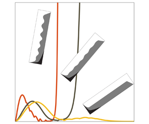
Many engineering processes apply tilted liquid columns to accelerate the separation of suspended materials. For example, in sewage systems, heavy wastes can be quickly removed from water columns when placed in inclined tanks (Smith & Davis Reference Smith and Davis2013). Typically, centrifuge systems are also designed with centrifuge tubes tilted at certain angles, such that fine suspended materials can be efficiently separated from the carrier fluid (Al-Faqheri et al. Reference Al-Faqheri, Thio, Qasaimeh, Dietzel, Madou and Al-Halhouli2017). In such apparatus, the Boycott effect, which was first reported by Boycott (Reference Boycott1920), plays a key role in sedimentation enhancement. The Boycott effect is a free-convection phenomenon driven by the density difference between particle-free and particle-laden fluid layers. As shown in figure 1, in a tilted water column, when a particle-laden fluid layer descends due to the gravity-induced settlement of particles, a thin layer of clear fluid (i.e. particle-free liquid layer) forms immediately beneath the downward-facing wall of the liquid column (see figure 1b). The presence of the clear-fluid layer, which does not occur in non-tilted cases (see figure 1a), has a buoyant effect, such that the clear fluid moves toward the top of the water column along the wall (see figure 1b). The resulting convective motion then pushes the suspension layer (i.e. particle-laden layer) toward the bottom of the water column, accelerating the sedimentation of suspended fine materials.

Figure 1. Schematic showing the sedimentation of fine particles in a liquid column (a) without inclination and (b) inclined at an angle  $\theta$, in which the white area represents the clear-fluid layer, the grey area is the suspension layer and the black area is the deposition layer. In the liquid columns, the black arrows indicate the settling of the particles and the grey arrow indicates the direction of the resulting convective flow.
In 1979, Acrivos & Herbolzheimer first developed a theoretical model to describe the hydrodynamic processes associated with the Boycott effect inside an inclined tube. Under the assumptions of a Newtonian fluid, Boussinesq approximation and a small-particle Reynolds number, Acrivos & Herbolzheimer (Reference Acrivos and Herbolzheimer1979) showed that the flow is dominated by three dimensionless parameters,
 \begin{equation} R \equiv \frac{H v_0 \rho}{\mu},\quad \varLambda \equiv \frac{H^2 g (\rho_s - \rho)c_0}{\mu v_0 },\quad \xi \equiv R^3 \varLambda^{{-}1} x \tan{\theta} \sin^3{\theta}, \end{equation}
where  $H$ is the vertical height of the suspension, $v_0$ is the settling velocity of the particles, $\theta$ is the inclined angle, $\rho$ is the fluid density, $\mu$ is the fluid viscosity, $g$ is the gravitational acceleration, $\rho _s$ is the particle density, $c_0$ is the initial volume fraction of the suspension and $x$ is the coordinate normalised by $H$ on the axis along the inlined plate (see figure 1b). In (1.1), $R$ is the sedimentation Reynolds number, $\varLambda$ is the ratio of the Grashof number to $R$ and $\xi$ is a parameter for quantifying the importance of the inertial effect (Shaqfeh & Acrivos Reference Shaqfeh and Acrivos1986). It was found that, at the limit of $\varLambda \rightarrow \infty$ and over the whole range of $R\varLambda ^{-1/3}$, the model obtains satisfactory results for settlers with a low aspect ratio (i.e. $b/H = {O}(1)$, where $b$ is the width of the tube) and in cases with a high aspect ratio with continuous settling, in which the suspension fluid is continuously supplied while the clear fluid is continuously removed from the settler. Although the model can be used to predict the accelerated sedimentation rate given by various physical parameters, such as the inclined angle, aspect ratio and initial particle concentration, sedimentation enhancement can be suppressed by flow instabilities owing to the strong shear generated at the interface between the clear-fluid and suspension layers. A shear instability leads to travelling waves at the particle-laden interface, which subsequently break and can be transformed into fine turbulent structures, which resuspend the sedimenting particles (Chang et al. Reference Chang, Chiu, Hung and Chou2019), thus reducing the enhanced sedimentation efficiency. In this regard, researchers have performed linear stability analysis to focus on the associated shear instabilities (Acrivos & Herbolzheimer Reference Acrivos and Herbolzheimer1979; Herbolzheimer & Acrivos Reference Herbolzheimer and Acrivos1981; Schneider Reference Schneider1982; Shaqfeh & Acrivos Reference Shaqfeh and Acrivos1986, Reference Shaqfeh and Acrivos1987b).
For a low-aspect-ratio regime, following the similarity solution and its asymptotic form for a highly viscous fluid ( $\xi ^{1/6}\rightarrow 0$) presented by Acrivos & Herbolzheimer (Reference Acrivos and Herbolzheimer1979), Herbolzheimer (Reference Herbolzheimer1983) further analysed the related interfacial instability. The author showed that most growing interfacial waves can be convected out of the channel without causing instabilities. In addition, he also found that among cases with various inclined angles and particle concentrations, the inception points of the interfacial waves and their associated amplifications are similar. Prasad (Reference Prasad1985) analysed flow instabilities for the inviscid case ( $\xi ^{1/6}\rightarrow \infty$) (Schneider Reference Schneider1982), and showed that flows can be stabilised by inertia and that particle concentration can damp dispersive waves at the interface.
In between the two extremes of  $\xi ^{1/6}$, cases with moderate $\xi ^{1/6}$ values were investigated by Shaqfeh & Acrivos (Reference Shaqfeh and Acrivos1986), who developed a theoretical model to describe the base flow using perturbation expansion. In their study, the flow field and the influence of flow inertia for different $\xi ^{1/6}$ values were analysed. Interfacial instabilities were also investigated by Shaqfeh & Acrivos (Reference Shaqfeh and Acrivos1987a) via linear stability analysis and the results were compared with the experimental results reported by Shaqfeh & Acrivos (Reference Shaqfeh and Acrivos1987b). They showed that $\xi ^{1/6}\sim O(1)$ results in the most unstable mode owing to the inviscid effect, and that this type of instability exists over the whole range of inclined angles. An important characteristic in low-aspect-ratio cases is that the thickness of a clear-fluid layer increases along the $x$-direction (Acrivos & Herbolzheimer Reference Acrivos and Herbolzheimer1979) (see figure 2a) and becomes thicker when $\xi ^{1/6}$ increases (Shaqfeh & Acrivos Reference Shaqfeh and Acrivos1986).

Figure 2. Schematic showing the sedimentation of particles in a tilted liquid column for cases with (a) low and (b) high aspect ratio, along with (c) a zoom-in figure of a two-layered flow in the fully developed section of a high-aspect-ratio case when the particle-laden interface is located at the middle in the  $y$-direction.
The studies by Herbolzheimer (Reference Herbolzheimer1983) and Shaqfeh & Acrivos (Reference Shaqfeh and Acrivos1987a) were concerned with the settling of small particles in a highly viscous fluid, such that the temporal change in the thickness of the clear-fluid layer owing to particle settling is negligible during the development of flow instabilities. Moreover, the non-uniform nature in the  $x$-direction of the base flow validates the linear modal stability analysis of spatially evolving disturbances for determining the criteria of wave formation in the quasi-steady state. This spatially varied clear-fluid layer can also be treated as a case in which particles slowly settle in liquid columns with a continuous settling mode in high-aspect-ratio containers (Herbolzheimer & Acrivos Reference Herbolzheimer and Acrivos1981; Davis, Herbolzheimer & Acrivos Reference Davis, Herbolzheimer and Acrivos1983; Leung & Probstein Reference Leung and Probstein1983). In the continuous settling mode, to maintain a time-invariant position of the interface, suspended particles are continuously fed into an inclined tube while clear fluids are withdrawn from the tube. As a result, the particle-laden interface in the base flow varies along the $x$-direction without temporal variation, such that the development of interfacial waves can be examined in the same way as in the low-aspect-ratio case. The base flow of the continuously settling mode was first proposed by Herbolzheimer & Acrivos (Reference Herbolzheimer and Acrivos1981), and the instability of the particle-laden interface was analysed by Davis et al. (Reference Davis, Herbolzheimer and Acrivos1983). However, the flow characteristics can differ significantly from high-aspect-ratio cases with no source and sink, namely the batch settling mode. This finding was first reported by Herbolzheimer & Acrivos (Reference Herbolzheimer and Acrivos1981) and Davis et al. (Reference Davis, Herbolzheimer and Acrivos1983), both of whom showed that in the batch settling mode, a clear-flow region with spatial variation only occupies a small portion of the water column, and most of the clear-fluid–suspension interface is nearly parallel to the downward-facing plate, as shown in figure 2(b). Chang et al. (Reference Chang, Chiu, Hung and Chou2019) confirmed these results in their numerical study. Moreover, owing to particle settling, the thickness of the clear-fluid layer increases with time, resulting in a change in the upward stream beneath the downward-facing wall, as shown in figure 2(b). These findings regarding the development of interfacial instabilities in high-aspect-ratio containers differ from those of previous studies, particularly those pertaining to cases with fast particle settling (i.e. large particle sizes or low liquid viscosity).
While the associated base-flow field has been studied by Herbolzheimer & Acrivos (Reference Herbolzheimer and Acrivos1981) and Amberg & Dahlkild (Reference Amberg and Dahlkild1987), instabilities in the batch settling mode have not been explored, even though they can be found in many industrial applications, such as in wastewater treatment (Sarkar, Kamilya & Mal Reference Sarkar, Kamilya and Mal2007) and ultracentrifugation in biochemistry studies (Schachman Reference Schachman2013). In this regard, this study aims to investigate the temporal evolution of flow disturbances in time-dependent base flows as particles settle in a tilted, long water column. Unlike the previous study by Davis et al. (Reference Davis, Herbolzheimer and Acrivos1983), who assumed a continuous particle supply to maintain a time-invariant particle-laden interface and steady state in the base flow (i.e. the continuous settling mode), we consider a descending interface due to particle settling and eliminate the assumption of the steady state for the base flow. By performing a non-modal stability analysis (Trefethen et al. Reference Trefethen, Trefethen, Reddy and Driscoll1993; Schmid Reference Schmid2007), we extend the application of the theoretical analysis for the Boycott effect to the more general case. To the best of our knowledge, this is the first study that focuses on the transient behaviour of flow instabilities associated with the Boycott effect in the batch settling mode in long tubes. We show that for the fast settling of particles, there is not enough time for the base flow to become fully developed and the associated stability problem is of an unsteady nature. Therefore, a settling time scale is introduced for the investigation of the transient behaviour of the base flow. The influence of settling speed on the magnitude of base flow is thus investigated. Two different stages of energy growth, namely the algebraic and exponential stages, in the time history are studied, and the main mechanisms leading to the flow instability in both stages are identified. Moreover, the optimal range of the tilted angle for efficient sedimentation is studied based on our stability analysis.
The rest of this paper is organised as follows. Section 2 presents a mathematical description of the problem, including the base flow, the evolution of the disturbance fields, and the measure used for the energy growth of the flow. Based on our numerical results, the effect of particle settling on the base flow is discussed in § 3. In § 4, we show the time history of the energy gain in a general case and present a detailed discussion of the growth in the energy gain during the stages of algebraic and exponential instabilities. We discuss the effect of the Prandtl number on the growth of the energy gain in § 6. In § 5, we consider the energy growth in different cases as a function of the Reynolds number, normalised particle settling speed and variations in disturbances. We then show the effect of the inclined angle in § 7 and discuss the applicability in § 8. Concluding remarks are then given in § 9.
2. Mathematical description of the problem
We assume that the suspended particles are sufficiently small that the buoyancy force is in balance with the Stokes drag and the particle inertia is negligible. Thus, the Eulerian description for the volume fraction of particles,  $\phi ^*$, can be expressed as
 \begin{equation} \dfrac{\textrm{D}^*}{\textrm{D}^* t^*}{\phi^*}+V_0^*\left(\boldsymbol{\nabla}^*\phi^*\boldsymbol{\cdot}\hat{\boldsymbol{e}}_g\right) = \kappa^* \nabla^{*2} \phi^*, \end{equation}
where  $\textrm {D}^*/\textrm {D}^* t^*$ is the material derivative, $V_0^*$ is the Stokes settling speed obtained by the balance between the particle drag and buoyant force, $\hat {\boldsymbol {e}}_g$ is the unit direction vector of the gravitational acceleration $g^*$, $\kappa ^*$ is the diffusivity and the superscript $*$ indicates the dimensional quantity of the physical variables. Following Herbolzheimer & Acrivos (Reference Herbolzheimer and Acrivos1981), we assume a dilute suspension, such that the viscosity of the liquid phase is not altered by the presence of the suspended particles. As shown in the schematic in figure 2(b), for a water column with an inclined angle $\theta$, under the Boussinesq approximation, the mass and momentum equations are as follows:
 $$\begin{gather} \boldsymbol{\nabla}^*\boldsymbol{\cdot}\boldsymbol{u}^* = 0, \end{gather}$$
 $$\begin{gather}\frac{\textrm{D}^*}{\textrm{D}^* t^*}\boldsymbol{u}^* ={-}\frac{1}{\rho^*}\boldsymbol{\nabla}^* p^* + \boldsymbol{\nabla}^* \mathcal{B}^* + \nu^*\nabla^{*2}\boldsymbol{u}^*, \end{gather}$$
where  $p^*$ is the modified pressure term obtained by subtracting the hydrostatic pressure of the clear-fluid column from the total pressure field and $\boldsymbol {\nabla }^*\mathcal {B}^*$ is the body-force term written in a conservative form. After subtracting the hydrostatic pressure of the clear-fluid column, $\boldsymbol {\nabla }^*\mathcal {B}^*$ becomes the buoyant forcing due to $\phi ^*$ and can be written as
 \begin{equation} \mathcal{B}^* = \int^{\boldsymbol{x}^*}_{\boldsymbol{x}^*_0}\phi^* g^{\prime *}(\check{\boldsymbol{x}}^*) \hat{\boldsymbol{e}}_g\boldsymbol{\cdot} \textrm{d}\check{\boldsymbol{x}}^{*}, \end{equation}
where  $\boldsymbol {x}^* = (x^*, y^*, z^*)$, $\boldsymbol {x}_0^*$ represents the reference position, $g^{\prime *} = (\rho _s^*/\rho ^*-1)g^*$ is the reduced gravity and $\hat {\boldsymbol {e}}_g = (-\cos {\theta }\hat {\boldsymbol {e}}_x, -\sin {\theta }\hat {\boldsymbol {e}}_y)$ represents the unit direction vector of $g^{\prime *}$ in the present configuration.
For the high-aspect-ratio case in which the liquid column is assumed to be fairly long in the  $x$-direction, we consider the fully developed flow section where the variations in the unperturbed momentum and concentration in the streamwise direction ( $x$) are zero. Without variation in both $x$- and $z$-directions (see figure 2b), the transport equation, (2.1), of $\phi ^*$ can be reduced to
 \begin{equation} \dfrac{\partial\phi^*}{\partial t^*}-V_0^*\sin\theta\dfrac{\partial \phi^*}{\partial y^*} = \kappa^*\dfrac{\partial^2\phi^*}{\partial y^{* 2}}. \end{equation}
It should be noted that in (2.5), if one considers only the molecular diffusivity, the value of  $\kappa ^*$ can be infinitesimally small according to the Stokes–Einstein equation. Examples are Herbolzheimer & Acrivos (Reference Herbolzheimer and Acrivos1981) and Davis et al. (Reference Davis, Herbolzheimer and Acrivos1983), in which the problem configurations become two fluid flows separated by a density jump. More recent studies have shown that additional ‘hydrodynamic diffusion’ exists owing to particle–particle and particle–hydrodynamics interactions, which can dominate the diffusion of the suspended particles over the molecular effect (e.g. Davis Reference Davis1996; Segre et al. Reference Segre, Liu, Umbanhowar and Weitz2001). However, hydrodynamic diffusion is still not a well-defined physical quantity and its magnitude can vary among different flow configurations. In this regard, different values of $\kappa ^*$ are studied in § 6, where we show that the instability characteristics asymptotically converge when $\kappa ^*$ becomes infinitesimally small. Typically, when the volume fraction of suspended particles is modelled using (2.5), the bottom boundary condition is specified as $V_0^* \phi ^* + \kappa ^* \partial \phi ^*/\partial y^* = 0$. However, this is usually the case where flow turbulence exists to support resuspension (e.g. Chou & Fringer Reference Chou and Fringer2008), and the diffusivity ( $\kappa ^*$) should be replaced by the eddy diffusivity. In this study, turbulence is not considered and, because $\kappa ^*$ is typically very small, the bottom wall is a deposition-dominant regime such that at the bottom boundary $V_0^* \phi ^* + \kappa ^* \phi ^*/\partial y^* > 0$ becomes deposition.
If the problem starts from a fully suspended water column with a volume fraction  $c_0^*$, the layer of deposition is usually thin and its thickness is negligible relative to the domain width (i.e. $\delta _d = 0$ in figure 2b). Therefore, we only consider the layer in which $\phi ^* \leqslant c_0^*$ (the grey areas in figure 2) as the particle-laden liquid column, which eliminates the complexities while dealing with the transition to the dense deposition zone on the wall. Under this condition, because $\phi ^*$ is uniform within the suspension layer in our domain of interest except at the diffusive interface where $0 < \phi ^* \leqslant c_0^*$, $\kappa ^* \partial \phi ^*/\partial y^*$ becomes zero on the bottom boundary. Thus, the bottom boundary condition for solving (2.5) in this study is to specify a flux $-V_0^*\phi ^*$, such that $\phi ^*$ at the bottom remains as $c^*_0$, except when the diffusive interface (i.e. $\phi ^* < c^*_0$) approaches the bottom boundary near the end of the calculation. In fact, starting from a fully suspended water column with a volume fraction $c_0^*$, using the boundary conditions $\phi ^* = 0$ at the top ( $y^* = b^*$) and specifying a flux $-V_0^*\phi ^*$ at the bottom, solving (2.5) (Ogata & Banks Reference Ogata and Banks1961) gives a descending diffusive interface specified by a time-varying error function given by
 \begin{equation} \phi^*(\zeta^*) = \dfrac{1 - \mathrm{erf}\left(\dfrac{\zeta^*}{2}\right)}{2}c_0^*, \end{equation}
where
 \begin{equation} \zeta^*\left(y^*, t^*\right) = \dfrac{y^*-b^*+V_0^*\sin\theta t^*}{\sqrt{\kappa^* t^*}}. \end{equation}
2.1. Scaling
The velocity scale is obtained by calculating the upper limit of the velocity magnitude for the undisturbed flow field in the steady state under the condition that both  $\kappa ^*$ and $V_0^*$ are zero and that the interface is located at the middle of the vertical dimension (i.e. $y^* = 0.5 b^*$). Assuming a fully developed, steady undisturbed flow (i.e. $\partial \boldsymbol {u}^*/\partial x^* = 0$) without any variation in the $z$-direction, as shown in figure 2(c), the governing equations can be reduced to a momentum equation in the $x$-direction of a planar flow written as
 $$\begin{gather} 0 ={-}\dfrac{\partial p^*}{\partial x^*}-\phi^*g^{\prime *}\cos\theta+\nu^*\dfrac{\partial^2 u^*}{\partial y^{* 2}}, \end{gather}$$
 $$\begin{gather}0 ={-}\dfrac{\partial p^*}{\partial y^*}-\phi^*g^{\prime *}\sin\theta, \end{gather}$$
where
 \begin{equation} \phi^* =
\left\{\begin{array}{@{}ll} c^*_0 & \mbox{if}\ 0\leqslant
y^*<\dfrac{b^*}{2}\\ 0 & \mbox{if}\ \dfrac{b^*}{2}\leqslant
y^*< b^* \end{array},\right.
\end{equation}
\begin{equation} \phi^* =
\left\{\begin{array}{@{}ll} c^*_0 & \mbox{if}\ 0\leqslant
y^*<\dfrac{b^*}{2}\\ 0 & \mbox{if}\ \dfrac{b^*}{2}\leqslant
y^*< b^* \end{array},\right.
\end{equation}
That is, the flow, governed by (2.8) and (2.9), becomes a two-layered flow separated by the interface of  $\phi ^*$ (see figure 2c).
For a water column with a long but finite length in the  $x$-direction, owing to the existence of end walls in the $x$-direction, the net flow at each cross-section must be zero. By imposing this zero-net-flow condition at the cross-section, along with the no-slip boundary condition at the walls and continuity for $u^*$ and stress ( $\nu ^* \partial u^*/\partial x^*)$ at the interface ( $y^* = b^*/2$), the solution can be obtained as
 \begin{equation} u^* = \left\{
\begin{array}{@{}ll} \dfrac{1}{4\nu^*}c_0^*g^{\prime
*}\cos\theta\left(y^{*2}-\dfrac{b^*}{2}y^{*}\right) &
\mbox{if}\ 0 \leqslant y^* < \dfrac{b^*}{2}\\
\dfrac{1}{4\nu^*}c_0^*g^{\prime
*}\cos\theta\left({-}y^{*2}+\dfrac{3b^*}{2}y^{*}-\dfrac{b^{*
2}}{2}\right) & \mbox{if}\ \dfrac{b^*}{2} \leqslant y^* <
b^* \end{array},\right.
\end{equation}
\begin{equation} u^* = \left\{
\begin{array}{@{}ll} \dfrac{1}{4\nu^*}c_0^*g^{\prime
*}\cos\theta\left(y^{*2}-\dfrac{b^*}{2}y^{*}\right) &
\mbox{if}\ 0 \leqslant y^* < \dfrac{b^*}{2}\\
\dfrac{1}{4\nu^*}c_0^*g^{\prime
*}\cos\theta\left({-}y^{*2}+\dfrac{3b^*}{2}y^{*}-\dfrac{b^{*
2}}{2}\right) & \mbox{if}\ \dfrac{b^*}{2} \leqslant y^* <
b^* \end{array},\right.
\end{equation}
which gives a two-layered flow in counter directions. Substituting  $y^* = b^*/4$ into the top identity or $y^* = 3b^*/4$ into the bottom identity of (2.11), the maximum magnitude of the velocity can be found as $c_0^*g^{\prime *} b^{* 2}\cos \theta / (64\nu ^*)$. Thus, we use
 \begin{equation} U_c^* = \frac{c_0^*g^{\prime *} b^{* 2}}{64\nu^*} \end{equation}
as the velocity scale of the present study.
For an inclined water column associated with a long dimension in the  $x$-direction, we use $b^*$, the domain length in the $y$-direction (see figure 2b), as our characteristic length scale, $U_c^*$ (2.12) as the velocity scale, $\mu ^* U_c^*/ b^*$ as the pressure scale and $c_0^*$ as the scale for the volume fraction. Substituting these dimensional parameters into (2.1)–(2.4) gives the dimensionless transport equation of $\phi$, written as
 \begin{equation} \frac{\partial \phi}{\partial t} + \left(\boldsymbol{u}-R_v\sin{\theta}\hat{\boldsymbol{e}}_y\right)\boldsymbol{\cdot}\boldsymbol{\nabla}\phi = \frac{1}{RePr}\nabla^2\phi, \end{equation}
and the dimensionless mass and momentum equations for the fluid, written as
 $$\begin{gather} \boldsymbol{\nabla}\boldsymbol{\cdot}\boldsymbol{u} = 0, \end{gather}$$
 $$\begin{gather}\frac{\partial}{\partial t}\boldsymbol{u} + \boldsymbol{u}\boldsymbol{\cdot}\boldsymbol{\nabla}\boldsymbol{u} ={-}\frac{1}{Re}\boldsymbol{\nabla} p + \boldsymbol{\nabla}\int^{\boldsymbol{x}}_{\boldsymbol{x}_0} \frac{64}{Re}\phi\hat{\boldsymbol{e}}_g\boldsymbol{\cdot} \textrm{d} \check{\boldsymbol{x}} + \frac{1}{Re}\nabla^2\boldsymbol{u}, \end{gather}$$
where
 \begin{equation} Re = \frac{U_c^* b^*}{\nu^*},\quad R_v = \frac{V^*_0}{U_c^*}, \quad \mbox{and}\quad Pr = \frac{\nu^*}{\kappa^*}, \end{equation}
are the Reynolds number, velocity ratio and Prandtl number, respectively.
2.2. Specification of time-dependent base flow
Each physical variable is expressed as a summation of its base state and perturbation, which can be written as
 \begin{equation}
\left.\begin{array}{rclcr@{}} \displaystyle u(x,y,z,t) & = &
U(y,t) & + & \tilde{u}(x,y,z,t), \\ v(x,y,z,t) & = & & &
\tilde{v}(x,y,z,t), \\ w(x,y,z,t) & = & & &
\tilde{w}(x,y,z,t), \\ p(x,y,z,t) & = & P(x,y,t) & + &
\tilde{p}(x,y,z,t), \\ \phi(x,y,z,t) & = & \varPhi(y,t) & +
& \tilde{\phi}(x,y,z,t). \end{array}\right\}
\end{equation}
\begin{equation}
\left.\begin{array}{rclcr@{}} \displaystyle u(x,y,z,t) & = &
U(y,t) & + & \tilde{u}(x,y,z,t), \\ v(x,y,z,t) & = & & &
\tilde{v}(x,y,z,t), \\ w(x,y,z,t) & = & & &
\tilde{w}(x,y,z,t), \\ p(x,y,z,t) & = & P(x,y,t) & + &
\tilde{p}(x,y,z,t), \\ \phi(x,y,z,t) & = & \varPhi(y,t) & +
& \tilde{\phi}(x,y,z,t). \end{array}\right\}
\end{equation}
Substitution of (2.17) into (2.13)–(2.15) yields equations describing the base flow and the temporal evolution of disturbances. The base-flow equation is as follows:
 $$\begin{gather} \dfrac{\textrm{d} U}{\textrm{d} x} = 0\,, \end{gather}$$
 $$\begin{gather}\frac{\partial U}{\partial t} ={-}\frac{1}{Re}\frac{\partial P}{\partial x} - \frac{64}{Re}\cos{\theta}\varPhi + \frac{1}{Re}\frac{\partial^2 U}{\partial y^2} , \end{gather}$$
 $$\begin{gather}0 ={-}\frac{1}{Re}\frac{\partial P}{\partial y} - \frac{64}{Re} \sin{\theta}\varPhi , \end{gather}$$
 $$\begin{gather}\frac{\partial \varPhi}{\partial t} - R_v\sin{\theta}\frac{\partial\varPhi}{\partial y} = \frac{1}{RePr}\frac{\partial^2\varPhi}{\partial y^2}, \end{gather}$$
where  $y \in [0, 1]$. Starting from a water column fully occupied by particle-laden fluid (i.e. $\varPhi (y, 0) = 1$), using the normalised boundary conditions, $\varPhi = 0$ at $y = 1$ and the mass flux $= -\varPhi R_v\sin \theta$ at the bottom wall, the solution of (2.21) can be simply obtained as
 \begin{equation} \varPhi(\zeta) = \frac{1-\mathrm{erf}\left(\dfrac{\zeta}{2}\right)}{2}, \end{equation}
where
 \begin{equation} \zeta(y, t) = \frac{\sqrt{PrRe} \left(y - 1 + R_v \sin{\theta} t\right)}{\sqrt{t}}. \end{equation}
To obtain the base flow  $U$ by solving (2.19), we note the net flow at each cross-section must be zero, as previously mentioned in § 2.1. That is, using the forcing owing to the time-varying $\varPhi$ given by (2.22), with the no-slip boundary condition at both the bottom and top walls and the condition of zero net flow in the cross-section, one can obtain the time-varying base-flow solution ( $U$) by solving (2.19) numerically. Here, we use the second-order central difference for spatial discretisation and second-order Crank–Nicolson method for time discretisation to obtain $U(y, t)$.
2.3. Temporal evolution of disturbances
In this study, we examine the transient instability by measuring the growth of the total energy, including the kinetic and potential energies. The kinetic energy can be obtained from the wall-normal velocity and the wall-normal vorticity (Schmid & Henningson Reference Schmid and Henningson2001; Schmid Reference Schmid2007), the potential energy in a generalised form (South & Hooper Reference South and Hooper1999; Sameen & Govindarajan Reference Sameen and Govindarajan2007; Jerome et al. Reference Jerome, Chomaz and Huerre2012) can be converted from the volume fraction  $\phi$. Let a state vector of disturbances, $\tilde {\boldsymbol {q}}$, be composed of disturbances of the wall-normal velocity $\tilde {v}$, wall-normal vorticity $\tilde {\eta }$ and volume fraction $\tilde {\phi }$. The energy of these disturbances can be defined as a weighted energy norm written as
 \begin{equation} \langle \tilde{\boldsymbol{q}}, \tilde{\boldsymbol{q}} \rangle_E = \tilde{\boldsymbol{q}}^H\boldsymbol{\mathsf{E}}\tilde{\boldsymbol{q}}, \end{equation}
where
 \begin{equation} \tilde{\boldsymbol{q}}
= \left[\begin{array}{@{}c@{}} \tilde{v}\\ \tilde{\eta}\\
\tilde{\phi} \end{array} \right],\quad
\boldsymbol{\mathsf{E}} = \left[ \begin{array}{@{}ccc@{}}
\dfrac{1}{2k^2}\left(k^2 - \mathcal{D}^2\right) & 0 & 0 \\
0 & \dfrac{1}{2k^2} & 0\\ 0 & 0 & \dfrac{1}{2}RePr
\end{array}\right],\quad k = \sqrt{\alpha^2 + \beta^2}
\end{equation}
\begin{equation} \tilde{\boldsymbol{q}}
= \left[\begin{array}{@{}c@{}} \tilde{v}\\ \tilde{\eta}\\
\tilde{\phi} \end{array} \right],\quad
\boldsymbol{\mathsf{E}} = \left[ \begin{array}{@{}ccc@{}}
\dfrac{1}{2k^2}\left(k^2 - \mathcal{D}^2\right) & 0 & 0 \\
0 & \dfrac{1}{2k^2} & 0\\ 0 & 0 & \dfrac{1}{2}RePr
\end{array}\right],\quad k = \sqrt{\alpha^2 + \beta^2}
\end{equation}
the superscript  $H$ denotes the Hermitian transpose, $\boldsymbol{\mathsf{E}}$ is the energy conversion matrix, $\alpha$ is the streamwise wavenumber, $\beta$ is the spanwise wavenumber and $\mathcal {D}^2 = \textrm {d}^2/{\textrm {d}y}^2$ ( $\mathcal {D} = \textrm {d}/{\textrm {d} y}$). Given that any disturbance input can be amplified differently with time, we are interested in initial perturbations that lead to maximum amplification. Therefore, we are interested in finding the initial disturbances that generate the optimal energy gain, $G_n(t; t_0)$, at each time point. The optimal energy gain within a time interval $[t_0, t]$ can be described as
 \begin{equation} G_n(t; t_0) = \mathop{\arg\max}\limits_{\tilde{\boldsymbol{q}}(t_0)}\frac{\langle \tilde{\boldsymbol{q}}(t), \tilde{\boldsymbol{q}}(t) \rangle_E}{\langle \tilde{\boldsymbol{q}}(t_0), \tilde{\boldsymbol{q}}(t_0)\rangle_E} = \mathop{\arg\max}\limits_{\tilde{\boldsymbol{q}}_0}\frac{\langle \tilde{\boldsymbol{q}}, \tilde{\boldsymbol{q}} \rangle_E}{\langle \tilde{\boldsymbol{q}}_0, \tilde{\boldsymbol{q}}_0\rangle_E}. \end{equation}
The resulting optimisation problem can be solved by propagating the disturbances forward and backward in time using the governing and corresponding adjoint equations (Farrell & Moore Reference Farrell and Moore1992; Schmid Reference Schmid2007; Luchini & Bottaro Reference Luchini and Bottaro2014).
The normal mode formulation for the components of  $\tilde {\boldsymbol {q}}$ (2.24) is written as
 \begin{equation} \begin{bmatrix}
\tilde{v}\\ \tilde{\eta}\\ \tilde{\phi}
\end{bmatrix} =\begin{bmatrix}
\hat{v}(y,t)\\ \hat{\eta}(y,t)\\ \hat{\phi}(y,t)
\end{bmatrix} \exp{\mathrm{i}(\alpha x + \beta z)}.
\end{equation}
\begin{equation} \begin{bmatrix}
\tilde{v}\\ \tilde{\eta}\\ \tilde{\phi}
\end{bmatrix} =\begin{bmatrix}
\hat{v}(y,t)\\ \hat{\eta}(y,t)\\ \hat{\phi}(y,t)
\end{bmatrix} \exp{\mathrm{i}(\alpha x + \beta z)}.
\end{equation}
Based on Equations (A9), (A12), and (A13) derived in Appendix A, the evolution of the disturbance field can be obtained by solving the Orr–Sommerfeld equation with baroclinic forcing, the Squire equation and the transport equation in a compact notation, written as follows:
 \begin{equation} \left(\boldsymbol{\mathsf{M}}\frac{\partial}{\partial t} - \boldsymbol{\mathsf{L}}\right)\hat{\boldsymbol{q}} = 0, \end{equation}
with
 \begin{equation}
\boldsymbol{\mathsf{M}} = \begin{bmatrix}
\mathcal{D} - k^2 & 0 & 0 \\ 0 & 1 & 0 \\ 0 & 0 & 1
\end{bmatrix} \quad\mbox{and}\quad
\boldsymbol{\mathsf{L}} = \begin{bmatrix}
\mathcal{L}_{OS} & 0 & \mathcal{L}_{Cv} \\
\mathcal{L}_{C\eta} & \mathcal{L}_{SQ} & 0 \\
\mathcal{L}_{C\phi} & 0 & \mathcal{L}_{\phi} \end{bmatrix},
\end{equation}
\begin{equation}
\boldsymbol{\mathsf{M}} = \begin{bmatrix}
\mathcal{D} - k^2 & 0 & 0 \\ 0 & 1 & 0 \\ 0 & 0 & 1
\end{bmatrix} \quad\mbox{and}\quad
\boldsymbol{\mathsf{L}} = \begin{bmatrix}
\mathcal{L}_{OS} & 0 & \mathcal{L}_{Cv} \\
\mathcal{L}_{C\eta} & \mathcal{L}_{SQ} & 0 \\
\mathcal{L}_{C\phi} & 0 & \mathcal{L}_{\phi} \end{bmatrix},
\end{equation}
where
 $$\begin{gather} \mathcal{L}_{OS} = \frac{1}{Re}(\mathcal{D}^2-k^2)^2 - \mathrm{i}\alpha U(\mathcal{D}^2-k^2) + \mathrm{i}\alpha \mathcal{D}^2U, \end{gather}$$
 $$\begin{gather}\mathcal{L}_{Cv} ={-}\frac{64}{Re}k^2\sin{\theta}, \end{gather}$$
 $$\begin{gather}\mathcal{L}_{C\eta} ={-}\mathrm{i}\beta\mathcal{D}U, \end{gather}$$
 $$\begin{gather}\mathcal{L}_{SQ} = \frac{1}{Re}(\mathcal{D}^2-k^2) - \mathrm{i}\alpha U, \end{gather}$$
 $$\begin{gather}\mathcal{L}_{C\phi} ={-}\mathcal{D}\varPhi, \end{gather}$$
 $$\begin{gather}\mathcal{L}_{\phi} = \frac{1}{RePr} (\mathcal{D}^2 - k^2) - \mathrm{i}\alpha U + R_v\sin\theta \mathcal{D}. \end{gather}$$
Because all disturbance quantities vanish on the walls, boundary conditions are given with
 \begin{equation} \hat{v} = 0, \quad \mathcal{D}\hat{v} = 0, \quad \hat{\eta} = 0, \quad \hat{\phi} = 0 \quad\mbox{on}\ \partial\varOmega_y, \end{equation}
where  $\partial \varOmega _y$ denotes the boundaries in the $y$-direction. It should be noted that the boundary condition $\hat {\phi } = 0$ on $\partial \varOmega _y$ is not consistent with the condition for the base flow, where we specify a flux for transport of the volume fraction at the bottom boundary. However, as we also solve for a set of adjoint equations in what follows, a flux-type boundary condition makes it very difficult to obtain its adjoint counterpart. In addition, because the instabilities of the momentum and volume fraction of particles are fully coupled, we set $\hat {\phi } = 0$ at the bottom boundary because of vanishing momentum disturbance in (2.31). Here, $\hat {\boldsymbol {q}}$ at time $t$ can be linked to the initial disturbance $\hat {\boldsymbol {q}}_0$ at time $t_0$ by an evolution matrix $\boldsymbol{\mathsf{A}}(t)$,
 \begin{equation} \hat{\boldsymbol{q}} = \boldsymbol{\mathsf{A}}(t)\hat{\boldsymbol{q}}_0, \end{equation}
which represents the time integration of (2.28) from the initial time  $t_0$ to a later time $t$. Equation (2.26) can then be rewritten as follows:
 \begin{equation} G_n(t; t_0) =
\mathop{\arg\max}\limits_{\tilde{\boldsymbol{q}}_0}\frac{\langle
\tilde{\boldsymbol{q}}, \tilde{\boldsymbol{q}}
\rangle_E}{\langle \tilde{\boldsymbol{q}}_0,
\tilde{\boldsymbol{q}}_0\rangle_E} =
\mathop{\arg\max}\limits_{\hat{\boldsymbol{q}}_0}\frac{\langle\boldsymbol{\mathsf{A}}(t)\hat{\boldsymbol{q}}_0,
\boldsymbol{\mathsf{A}}(t)\hat{\boldsymbol{q}}_0
\rangle_E}{\langle \hat{\boldsymbol{q}}_0,
\hat{\boldsymbol{q}}_0\rangle_E} =
\mathop{\arg\max}\limits_{\hat{\boldsymbol{q}}_0}\frac{\langle\boldsymbol{\mathsf{A}}^{{\dagger}}(t)\boldsymbol{\mathsf{A}}(t)\hat{\boldsymbol{q}}_0,
\hat{\boldsymbol{q}}_0 \rangle_E}{\langle
\hat{\boldsymbol{q}}_0, \hat{\boldsymbol{q}}_0\rangle_E},
\end{equation}
\begin{equation} G_n(t; t_0) =
\mathop{\arg\max}\limits_{\tilde{\boldsymbol{q}}_0}\frac{\langle
\tilde{\boldsymbol{q}}, \tilde{\boldsymbol{q}}
\rangle_E}{\langle \tilde{\boldsymbol{q}}_0,
\tilde{\boldsymbol{q}}_0\rangle_E} =
\mathop{\arg\max}\limits_{\hat{\boldsymbol{q}}_0}\frac{\langle\boldsymbol{\mathsf{A}}(t)\hat{\boldsymbol{q}}_0,
\boldsymbol{\mathsf{A}}(t)\hat{\boldsymbol{q}}_0
\rangle_E}{\langle \hat{\boldsymbol{q}}_0,
\hat{\boldsymbol{q}}_0\rangle_E} =
\mathop{\arg\max}\limits_{\hat{\boldsymbol{q}}_0}\frac{\langle\boldsymbol{\mathsf{A}}^{{\dagger}}(t)\boldsymbol{\mathsf{A}}(t)\hat{\boldsymbol{q}}_0,
\hat{\boldsymbol{q}}_0 \rangle_E}{\langle
\hat{\boldsymbol{q}}_0, \hat{\boldsymbol{q}}_0\rangle_E},
\end{equation}
where the superscript  ${{\dagger}}$ denotes the adjoint operator and $\boldsymbol{\mathsf{A}}^{{\dagger}} (t)$ is the evolution matrix of the associated adjoint equation:
 \begin{equation} \left(-\boldsymbol{\mathsf{M}}^{{\dagger}}\frac{\partial}{\partial t} - \boldsymbol{\mathsf{L}}^{{\dagger}}\right)\hat{\boldsymbol{q}}^+= 0, \end{equation}
where the superscript  $+$ denotes the complex conjugate. We note that in (2.28), $\boldsymbol{\mathsf{M}}$ is a self-adjoint operator, such that $\boldsymbol{\mathsf{M}}^{{\dagger}} = \boldsymbol{\mathsf{M}}$ in (2.34). The boundary conditions for the solutions of (2.34) are
 \begin{equation} \hat{v}^+= 0, \quad \mathcal{D}\hat{v}^+= 0, \quad \hat{\eta}^+= 0, \quad \hat{\phi}^+= 0 \quad\mbox{on}\ \partial\varOmega_y. \end{equation}
The last identity in (2.33) implies that finding an initial disturbance that causes the maximum gain is equivalent to seeking an eigenvector that corresponds to the maximum eigenvalue of  $\boldsymbol{\mathsf{A}}^{{\dagger}} (t)\boldsymbol{\mathsf{A}}(t)$. This can be accomplished by solving the ordinary differential equation system composed of (2.28) and (2.34). This process begins from guessing an initial, random disturbance field $\hat {\boldsymbol {q}}_0$ at the initial time $t_0$. The initial disturbance is propagated to a later time $t$ using (2.28) with an appropriate time-marching scheme. The resulting disturbance at $t$ is then propagated back to $t_0$ using (2.34). Variations in the resulting disturbance and energy gain between two consecutive loops decrease as the number of loops increases. For details of the computational procedure used, readers are referred to Schmid & Brandt (Reference Schmid and Brandt2014). In our case, the termination criterion for the iterations is that the relative variation between two consecutive loops needs to be less than $10^{-5}$. Equation (2.28) and its adjoint form (2.34) are evolved using the Chebyshev collocation method (Weideman & Reddy Reference Weideman and Reddy2000; Trefethen Reference Trefethen2019) in space and the second-order marching scheme in time accompanied by the implicit Euler method as a starter following Hack & Zaki (Reference Hack and Zaki2015). The $(n+1)$th step of the state vector is thus calculated using
 \begin{equation} \hat{\boldsymbol{q}}^{(n+1)} = (3\boldsymbol{\mathsf{M}}-2\Delta t\boldsymbol{\mathsf{L}}^{(n+1)})^{{-}1}\left(\boldsymbol{\mathsf{M}}\left(4\hat{\boldsymbol{q}}^{(n)}-\hat{\boldsymbol{q}}^{(n-1)}\right)\right). \end{equation}
We adopted Chebyshev points of the second kind to discretise the physical domain in the wall-normal direction. As the spectral grids are defined within the interval  $[-1,1]$, the derivative with respect to $y$ must be stretched by a factor of two. To impose $m$ boundary constraints, an $N$-point second-kind Chebyshev polynomial interpolant of order $N$ is downsampled on to an $N$-point first-kind Chebyshev polynomial interpolant of order $(N-m)$, which excludes the boundary points at $y = \pm 1$. In this way, an $N$-by- $N$ differentiation matrix becomes an $(N-m)$-by- $N$ matrix, whose vanishing rows are then replenished by the boundary information, following the work of Driscoll & Hale (Reference Driscoll and Hale2016) and Trefethen (Reference Trefethen2019).
Computations were performed using the Julia programming language (Bezanson et al. Reference Bezanson, Edelman, Karpinski and Shah2017), and the packages of Cairo.jl (Bezanson et al. Reference Bezanson, Fischer, Holy, Nolta and Shah2012), Dierckx.jl (Barbary et al. Reference Barbary, Sundar and Ortner2020), FFTW.jl (Frigo & Johnson Reference Frigo and Johnson2005), Makie.jl (Danisch et al. Reference Danisch and Krumbiegel2021), JLD.jl (Holy et al. Reference Holy, Hinsen, Short and Kornblith2020), Roots.jl (Verzani et al. Reference Verzani, Ignatiev and Rackauckas2021), SpecialFunctions.jl (Johnson et al. 2021), and ToeplitzMatrices.jl (Noack et al. Reference Noack, Olver and Xu2021).
3. Effect of particle settling on the base flow
In this section, we investigate changes in the base flow in response to a fast-settling, particle-laden layer. To examine this clearly, (2.19) is rearranged to become
 \begin{equation} \frac{\partial U}{\partial t} = \frac{1}{Re_s\sin{\theta}}\left(-\frac{\partial P}{\partial x} - 64\cos{\theta}\varPhi + \frac{\partial^2 U}{\partial y^2}\right), \end{equation}
where
 \begin{equation} Re_s = R_v Re = \frac{V_0^* b^*}{\nu^*} \end{equation}
is the sedimentation Reynolds number, which indicates the balance between particle settling and the viscous effect. In (3.1), we can see that, given a fixed inclined angle,  $\theta$, so that the buoyant forcing, $64\cos {\theta }\varPhi$, is fixed, $Re_s$ appears to be the only parameter that controls the base flow. Figure 3 presents profiles of the streamwise velocity for various $Re_s\sin {\theta }$ with $\theta = 30^\circ$, $Re = 215$, and $PrRe = 1000$ at ten time points, which show that typically, base flows of various $Re_s\sin {\theta }$ attain maximum speed at the time point at which the particle-laden interface reaches the middle of the domain in the vertical direction. However, as $Re_s\sin \theta$ increases (i.e. fast settling), the development of the base flow is somewhat delayed relative to the settlement of the particle-laden interface, as indicated by the grey lines in the figure. In figure 3, we can also see that the maximum speed the base flow can reach decreases as $Re_s\sin {\theta }$ increases. Moreover, the temporal development of the velocity profile converges with decreasing $Re_s\sin {\theta }$. In (3.1), $Re_s\sin \theta$ indicates how fast the flow can adapt to any change owing to the settlement of the particle-laden interface. If $Re_s\sin {\theta } \ll 1$, one anticipates a quasi-steady state in which the flow can adjust itself rapidly in response to the combined forcing of the pressure and buoyancy. In this case, the flow can attain its maximum strength at each time step. In contrast, when $Re_s\sin {\theta } \gg 1$, the flow cannot react instantly to the particle settling, so the flow develops after the descent of the particle-laden interface.

Figure 3. Time series of the streamwise velocity profiles for various  $Re_s\sin {\theta }$. The grey horizontal lines indicate positions of the particle-laden interface.
4. Energy growth of disturbances
For the sake of clarity, here, we first focus on a representative case with  $R_v = 0.01$, $Re = 215$, $PrRe = 1000$, $\theta = 30^\circ$ and $(\alpha, \beta ) = ({\rm \pi} /2, {\rm \pi}/2)$, which is denoted as the base case hereafter. In this case, values for $\alpha$ and $\beta$ are chosen such that both the algebraic and exponential instabilities can be clearly seen, as discussed in the following. Figure 4 presents time histories of various $G_n(t;t_0)$. In this figure, each curve represents different $G_n(t;t_0)$ resulting from the disturbances initialised at different time instants, $t_0$, during the early time stage (see inset (a)). Typically, the energy gain $G_n(t;t_0)$ undergoes algebraic growth and decay in the early stage (see inset (a) in figure 4), followed by a duration of stable flow development (i.e. $G_n(t;t_0) = 1$), and then exponential growth to a peak magnitude significantly greater than that of the early algebraic case. In the present cases, owing to the descent of the particle-laden interface, the buoyant forcing resulting from the particle-laden layer eventually vanishes, such that the flow energy always decays at the end. In figure 4, the time step $t = 215$ is the time point at which particles completely settle on to the upper-facing wall. Hereafter, we also consider the maximum amplification of the energy gain at time $T$ acquired from perturbations introduced at all time instants $t$ during the time interval $[t_0, T]$. Our focus is on the maximum energy gain, $G(t)$, caused by any disturbances, which is defined as follows (Blesbois et al. Reference Blesbois, Chernyshenko, Touber and Leschziner2013):
 \begin{equation} G(t) = \mathop{\arg\max}\limits_{t_0}{G_n}(t; t_0). \end{equation}
An example of  $G$ for the base case is highlighted by the black dash-dotted line in figure 4.

Figure 4. Time histories of the optimal energy gain  $G_n(t;t_0)$ in the base case with the disturbance initialised at different time points during the beginning stage (see inset (a)). The dash-dotted line indicates the corresponding maximum energy gain $G$ (4.1).
4.1. Algebraic growth
Figure 5 presents contours of the peak value of  $G_n(t;t_0)$ during the algebraic instability as a function of the streamwise and spanwise wavenumbers in cases wherein all other parameters are the same as those in the base case. In general, we can see that with a fixed $\beta$, the energy growth during the algebraic instability diminishes with increasing $\alpha$. The maximum growth is found at $\beta = 0.68$ when $\alpha = 0$. To examine the mechanism causing the algebraic instability, we set $\alpha = 0$, such that the governing differential equations, (2.27) and (2.28), become
 $$\begin{gather} (\mathcal{D}^2 - \beta^2) \displaystyle\frac{\partial}{\partial t} \hat{v} ={-}\frac{64}{Re}\beta^2\sin{\theta}\hat{\phi}+ \frac{1}{Re}(\mathcal{D}^2-k^2)^2\hat{v}, \end{gather}$$
 $$\begin{gather}\displaystyle\frac{\partial}{\partial t} \hat{\eta} ={-}\textrm{i}\beta\mathcal{D}U\hat{v} + \frac{1}{Re}(\mathcal{D}^2-k^2)\hat{\eta}, \end{gather}$$
 $$\begin{gather}\displaystyle\frac{\partial}{\partial t} \hat{\phi} ={-} R_v\sin{\theta}\mathcal{D}\hat{\phi} - \mathcal{D}\varPhi\hat{v} + \frac{1}{PrRe}(\mathcal{D}^2-k^2)\hat{\phi}. \end{gather}$$
At this point, one can see that the algebraic instability can be attributed to two potential contributions. The first possible contribution is the buoyant forcing (the first term in the right-hand side of (4.2), which can increase the magnitude of  $\hat {v}$. The second contribution is the possible growth in $\eta$ due to vortex tilting, also known as the lift-up mechanism (4.3) (Brandt Reference Brandt2014; Schmid & Brandt Reference Schmid and Brandt2014). To identify the dominant mechanism, figure 6 presents $G_n(t;t_0)$ and representative snapshots of streamlines on the $yz$-plane using $t_0 = 0.0$ in the case with $(\alpha, \beta ) = (0, {\rm \pi}/2)$, with all other parameters the same as those in the base case. In figure 6(b), we can see that the instability begins with perturbations that have a value of zero in the streamwise direction ( $\tilde {u} \approx 0$), but vary in the spanwise direction, which results in a pair of streamwise vortices. As shown in figure 6(c), when the peak of $G_n(t;t_0)$ is attained during algebraic instability (see figure 6a), the transverse perturbation components (shown by the streamlines) do not change appreciably, but $\tilde {u}$ significantly increases, which, with its spanwise variation, causes growth in $\tilde {\eta }$. Therefore, as consistently reported in the context of transient behaviours in shear instabilities (e.g. Brandt Reference Brandt2014; Schmid & Brandt Reference Schmid and Brandt2014), the energy growth during algebraic instability can be attributed to the lift-up mechanism.

Figure 5. Contours of the peak values of the maximum energy gain,  $G_n(t;t_0)$, during algebraic instability as a function of $\alpha$ and $\beta$ in cases where all other parameters are the same as those in the base case. The solid lines are contour lines starting at $100$ with increments of $100$.

Figure 6. (a) Time history of the development of the energy gain that yields the maximum energy growth ( $t_0 = 0$) in the case with $(\alpha, \beta ) = (0, {\rm \pi}/2)$, with all other parameters the same as in the base case during the algebraic instability and the corresponding disturbance flow field at (b) $t = 0$ and (c) $= 37$, the time point at which the energy growth reaches its local maximum. In (b,c), the flow field is presented by the colour contours of the streamwise component $\tilde {u}$ and the streamlines on the $yz$-plane, for which the solid and dashed lines indicate clockwise and counterclockwise rotation, respectively.
4.2. Exponential energy growth
As shown in figure 4,  $G_n(t;t_0)$ begins to increase when $t \approx 100$. The greatest exponential growth (see the pink line in figure 4) corresponds to the evolution of the perturbation initialised at $t_0 = 67.5$, which is approximately the time when the descending particle-laden interface reaches one third of the domain. That is, unlike the algebraic instability regime in which earlier $t_0$ leads to the greater and earlier growth of $G_n(t;t_0)$ (see the inset in figure 4), in the exponential growth regime, flow perturbations at the time point at which the interface reaches approximately one third of the domain produces optimal energy growth. This can be further examined from the energy equation, which is obtained by substituting (2.17) into (2.15), multiplying with $\hat {\boldsymbol {u}}$, and integrated over a control volume within a wave period, denoted as $\varOmega$. The resulting energy equation is expressed as
 \begin{equation} \displaystyle\frac{\textrm{d} }{\textrm{d} t} E ={-}\int_\varOmega \hat{u}\hat{v}\mathcal{D}U\,\textrm{d}\boldsymbol{x} - \frac{1}{Re}\int_\varOmega \left(\boldsymbol{\nabla} \times {\hat{\boldsymbol{u}}}\right)^2\,\textrm{d}\boldsymbol{x}, \end{equation}
where
 \begin{equation} E = \tfrac{1}{2}\int_\varOmega \hat{\boldsymbol{u}}\boldsymbol{\cdot} \hat{\boldsymbol{u}}\,\textrm{d} \boldsymbol{x} \end{equation}
is the kinetic energy of the disturbance. Moreover, substituting (2.17) into (2.13), multiplying with  $\hat {\phi }$, and integrating over a control volume within a wave period gives
 \begin{equation} \dfrac{\textrm{d}}{\textrm{d}t} E_{\hat{\phi}} ={-}\int_\varOmega \hat{\phi}\hat{v}\mathcal{D}\varPhi\,\textrm{d}\boldsymbol{x} - \frac{1}{PrRe} \int_\varOmega \boldsymbol{\nabla}\hat{\phi}\boldsymbol{\cdot}\boldsymbol{\nabla}\hat{\phi}\,\textrm{d} \boldsymbol{x}, \end{equation}
where
 \begin{equation} E_{\hat{\phi}} = \tfrac{1}{2}\int_\varOmega \hat{\phi}^2 \,\textrm{d}\boldsymbol{x} \end{equation}
is the generalised potential energy of the disturbances (South & Hooper Reference South and Hooper1999; Sameen & Govindarajan Reference Sameen and Govindarajan2007; Jerome et al. Reference Jerome, Chomaz and Huerre2012). In both (4.5) and (4.7), the first terms on the right-hand sides represent the energy production that transfers energy from the shear of the base flow, while the second terms on the right-hand sides of these two equations represent dissipation. Equations (4.5) and (4.7) clearly show that the energy of disturbances can grow due to the interaction between the base-flow shear and disturbance fields of momentum and concentration, respectively. The exponential growth of the flow energy is much stronger than that in the algebraic case and would dominate the flow instability throughout the descent of the particle-laden interface. Figure 7 shows the contours of the peak values of the maximum energy gain ( $G$) at various $\alpha$ and $\beta$ values in cases wherein all other parameters are the same as those in the base case. It can be seen that for a fixed $\alpha$, $G$ monotonically increases with decreasing $\beta$, which indicates that perturbations with a streamwise variation are most susceptible to the shear of the base flow, and the spanwise variation can stabilise the flow. Moreover, figure 7 shows that the most unstable case (i.e. greatest $G$) occurs at $\alpha \approx {\rm \pi}$, which means that the perturbation leading to the greatest amplification of energy has a wavelength which is comparable to twice the domain width, $b$, i.e. a vortex with the size of the domain width.

Figure 7. Contours of peak values of the maximum energy gain,  $G$, as a function of $\alpha$ and $\beta$ in cases wherein all other parameters are the same as those in the base case.
At this point, it is also interesting to investigate the evolution of the disturbance field in response to the descent of the particle-laden interface. We examine this in a case wherein all parameters are the same as those in the base case but for the setting  $(\alpha, \beta ) = ({\rm \pi} /2, 0)$. The panels in the upper row of figure 8 show five consecutive snapshots of the streamlines in the $yx$-plane at $z = 0.5$ at representative time points for the disturbance field with $t_0 = 0$. Initially, streamwise perturbations form counter-rotating pairs of spanwise vortices (i.e. $\tilde {\omega }_z$) along the $x$-direction. During the descent of the particle-laden interface, the upper panels in figure 8 show that the vortices in the upper layer (i.e. the clear-fluid layer) are distorted toward the left and those in the lower layer (i.e. the particle-laden layer) are distorted toward the right. This vortex distortion can be explained by the equation of the spanwise vorticity $\tilde {\omega }_z$, which is obtained by applying the curl operator to the momentum equations for disturbances (i.e. (A2)–(A4)). Neglecting the diffusion term, the temporal change of $\tilde {\omega }_z$ can be expressed as follows:
 \begin{equation} \frac{\partial \tilde{\omega}_z}{\partial t} + U\frac{\partial \tilde{\omega}_z}{\partial x} = \tilde{v}\mathcal{D}^2U. \end{equation}
Equation (4.9) shows that the temporal change of  $\tilde {\omega }_z$ at fixed spatial points is caused by transport by the base flow and the transfer from the vorticity of the base flow through the perturbation component $\tilde {v}$, i.e. $\tilde {v}\mathcal {D}^2 U$. Here, the second derivative of the base-flow velocity is typically one order of magnitude greater than the velocity itself. Therefore, unless the streamwise wavenumber $\alpha$ is high (e.g. ${>}O(10)$), the temporal change in $\tilde {\omega }_z$ is dominated by $\tilde {v}\mathcal {D}^2 U$. The panels in the lower row of figure 8 show contours of $\tilde {v}\mathcal {D}^2 U$ that correspond to the upper panels. Because $\mathcal {D}^2 U$ has different signs in the clear-fluid and particle-laden layers (see figure 3) and $\tilde {v}$ has the same sign throughout the $y$-direction, the $\tilde {u}\mathcal {D}^2 U$ field usually jumps to a different sign across the descending particle-laden interface, thus distorting the streamline patterns along the $y$-direction.

Figure 8. Consecutive snapshots of the streamlines in the  $yx$-plane (upper panels) of the disturbance flow field that leads to the maximum energy gain during exponential instability in the case wherein all of the parameters are the same as those in the base case except that $(\alpha, \beta ) = ({\rm \pi} /2, 0)$, and the corresponding contours of $\tilde {v}\mathcal {D}^2 U$ (lower panels).
5. Effect of  ${R}_{v}$ and $Re$ on disturbances


As presented in § 3, with fixed  $\theta$ and $Pr$ values, the combined effect of $R_v$ and $Re$ dominates the base flow, whereas the disturbance fields are dominated by $R_v$ and $Re$ separately (see (2.28)–(2.30)). In this section, we examine the energy gain as a function of $R_v$ and $Re$ in the exponential growth regime. As shown in the inset of figure 4, in the exponential regime of the present cases, once the energy begins to grow, $G_n(t; t_0)$ can easily reach $10^4$ and typically soon increases to $O(10^{6})$ in the case with the highest energy. Here, we set $G = 10^4$ as a criterion to distinguish between two regimes (i.e. $G > 10^4$ or $< 10^4$). Although, this criterion is somewhat arbitrary, we note that the overall trend that we present subsequently would not change if other values were adopted. Figure 9 presents the contours of $G = 10^4$ as a function of $\alpha$, $\beta$ and $R_v$, with fixed $Re$ ( ${=}215$) and $\theta$ ( ${=}30^\circ$ values). In the figure, the area enclosed by the contour is the regime in which $G > 10^4$, whereas outside the contour, $G < 10^4$. In figure 9, we can see that the area enclosed by the contour of $G = 10^4$ shrinks as $R_v$ increases. This enclosed area becomes zero when $R_v = 0.5$, which indicates the stabilising effect of the descent of the particle-laden interface, mainly because of the weakened base-flow field as $R_v$ increases, as discussed in § 3. The contours tend to remain unchanged as $R_v$ decreases (e.g. $R_v < 0.001$), which means that for given $Re$ and $\theta$ values, a maximum instability regime can be obtained with $R_v \rightarrow 0$.

Figure 9. Contour lines of  $G = 10^4$ as a function of $\alpha$ and $\beta$ for various $R_v$ in the cases wherein all other parameters are the same as those in the base case.
Figure 10 presents the contour lines of  $G = 10^4$ at $\alpha = 3.0$ as a function of $\beta$, $Re$ and $R_v$. Again, in this figure, the area beneath the contour line in each case represents the regime in which $G > 10^4$. Therefore, the smaller enclosed area with increasing $R_v$ indicates that the flow becomes more stable as particles settle faster, the same trend can also be seen in figure 9. Generally, with increasing $Re$, flows become unstable when certain threshold values of $Re$ are reached. However, in the cases with greater $R_v$ (e.g. $R_v \geqslant 0.028$), the contour lines in figure 10 imply that the flows become stabilised when $Re$ further increases (e.g. $Re > 500$). This is because during the transient stage, with the greater $Re$, it requires more time for the flow to be fully developed. In this case, the presence of the descending particle-laden interface hinders the development of the flow, such that the shear and resulting instability are suppressed.

Figure 10. Contour lines of  $G = 10^4$ as a function of $\beta$ and $Re$ with a fixed $\alpha = 3.0$ for various $R_v$ in cases wherein all other parameters are the same as those in the base case.
6. Effect of the Prandtl number on disturbances
In this section, we investigate the influence of the Prandtl number,  $Pr$. Figure 11 shows the time evolution of the maximum energy gain, $G(t)$, in the base case with various $Pr$. In this figure, each curve of $G(t)$ is obtained based on the collection of $G_n(t;t_0)$ values with disturbances initialised at $t_0$ ranging from $0$ to $204$ with an equal time spacing $\Delta t_0 = 10.75$. It can be seen that increasing $Pr$ results in an increase of $G(t)$. This is due to the fact that $PrRe$ controls the diffusion of mass transport, (2.30f). With a fixed $Re$, a higher $Pr$ leads to a sharper particle-laden interface in the base flow and higher energy dissipation in disturbances. Moreover, figure 11 shows that $G(t)$ converges with increasing $Pr$, which implies that when there are large particles in association with infinitesimal diffusivities, asymptotic results can be anticipated with increases in $Pr$.
$Pr$.

Figure 11. Time histories of the maximum energy gain  $G$ in cases with $PrRe$ varying from $1000$ to $9000$ and all other parameters being the same as those in the base case. Here, each curve of $G(t)$ is obtained based on the collection of $G_n(t;t_0)$ (see (4.1)) in which $t_0 \in [0, 204]$ with an increment $\Delta t_0 = 10.75$.
7. Influence of the inclined angle, ${\theta }$, on disturbances

In this section, we investigate the influence of the inclined angle,  $\theta$, on the energy growth of disturbances. In figure 12, we present the temporal evolution of the maximum energy gain, $G(t)$, in cases with various $\theta$. Because $\theta$ varies between cases, the total durations of all cases are different depending on $V_0^*\sin {\theta }$. Therefore, for easier comparison, we rescale the time by multiplying by $R_v \sin {\theta }$. In this way, the inclined angle is taken into account in the new time scale, and the new dimensionless time $tR_v \sin {\theta }$ represents the time relative to particle settling, i.e. $tR_v \sin {\theta } = 1$ when the particle laden layer ( $\varPhi = 1$) fully settles on to the bottom. In the figure, each curve of $G(t)$ is obtained based on the collection of $G_n(t;t_0)$ values with disturbances initialised at $t_0 R_v\sin {\theta }$, ranging from $0.0$ to $0.6$ with an equal time spacing $\Delta t_0 R_v\sin {\theta } = 0.05$. Figure 12 shows that increasing $\theta$ delays the development of energy growth, which is evident in aspects of both the algebraic and exponential growth. Moreover, the peak of $G(t)$ decreases with increases in $\theta$, except that when $\theta = 50^\circ$, no exponential growth occurs. These results are mainly due to the decrease in buoyant forcing in the momentum of the base flow when $\theta$ increases (see (2.19)), which reduces the generated velocity shear, thereby suppressing instability. Another important effect of $\theta$ is on the descending speed of the particle-laden interface. As shown in the second term on the left-hand side of (2.21), increasing $\theta$ yields higher descending speed of the particle-laden interface. As discussed in § 3, a high descending speed of the interface may restrict the base flow from reaching its quasi-steady state. As a result, the strength of the base flow decreases and the flow, thus, becomes more stable. Moreover, figure 12 shows that $G(t)$ dramatically decreases when $\theta$ becomes greater than $40^\circ$, indicating that flow instabilities are significantly suppressed. When $\theta$ further increases to $55^\circ$, it can be seen that values of $G(t)$ at $t R_v\sin {\theta } > 0.50$ are much reduced compared with all the other cases with smaller $\theta$. In fact, when $\theta = 55^\circ$, increase of $G(t)$ is only attributed to algebraic growth. This can be seen from figure 13, where we plot all curves of $G_n(t; t_0)$ that make $G(t)$ with $\theta = 55^\circ$ in figure 12. Each curve of $G_n(t; t_0)$ has either one or two peaks, in which the first peak corresponds to the algebraic growth and the second is due to the exponential growth. However, unlike the base case as shown in figure 4 where the exponential growth is much stronger, even the greatest value of the second peak of $G_n(t; t_0)$ in figure 13 (note the dash-dotted curve started at $t = 52$) is found to be much less than the first peak values of $G_n(t; t_0)$. Therefore, one may conclude that the flow can be significantly stabilised in its exponential regime when $\theta > 40^\circ$. At this point, it is worthwhile to mention that the previous numerical study by Chang et al. (Reference Chang, Chiu, Hung and Chou2019) suggested an optimal inclined angle $\theta _{op} = 40^\circ \text {--}50^\circ$ such that the sedimentation process can be accelerated to a maximum extent without causing flow instability. Moreover, an empirical value of ${\approx }45^\circ$ was suggested by the wastewater engineering practice (Kao Reference Kao1978) to reach the maximum separation efficiency. Our finding here seems to support these previous findings from different study approaches.

Figure 12. Time histories of the maximum energy growth with different  $\theta$ in cases wherein all other parameters are the same as those in the base case. Here, each curve of $G(t)$ is obtained based on the collection of $G_n(t;t_0)$ (see (4.1)) in which $t_0 R_v\sin {\theta } \in [0, 0.6]$ with an increment $\Delta t_0 R_v\sin {\theta } = 0.05$.

Figure 13. Time histories of all  $G_n(t; t_0)$ that make the curve of $G(t)$ with $\theta = 55^\circ$ in figure 12. The dash-dotted line denotes the curve associated with $t_0 = 52$, which shows two peaks of $G_n$. The thick grey line represents the curve of $G$ obtained based on the collection of the local maximum of all $G_n$ curves (4.1).
8. Applicability
It should be noted that in this study, an important assumption we have made is the small particle size, such that particles can soon reach their terminal speed and our scalar transport equation used to describe the volume fraction of particles is valid. This is the case when the particle relaxation time,  $\tau _p$, is small. For spherical particles, this means that $\tau _p^* = \rho _s^*d_0^{*2}/(18\mu ^*) \ll 1$, in which $d^*_0$ is the particle diameter. In liquid flows for which the $\mu \approx 10^{-3}\ \textrm {kg}\ \textrm {m}^{-1}\ \textrm {s}^{-1}$ (e.g. water) or greater, this can be easily met if the particle diameter $d_0 < O(1\ \mbox {mm})$, which is very common in suspension flows in various engineering and industrial applications (Galvin et al. Reference Galvin, Callen, Zhou and Doroodchi2005; Madge, Romero & Strand Reference Madge, Romero and Strand2005). Another assumption is that the particle concentration is dilute such that the viscosity cannot be significantly altered in the presence of suspended particles (see § 2). According to the theoretical work of Batchelor & Green (Reference Batchelor and Green1972), the flow viscosity can be significantly altered when the volume fraction $\phi ^*$ is $O(0.1)$. Therefore, the applicability of the present findings can be extended to suspension liquids in which $\phi ^* < 0.1$. However, even when $\phi ^*$ is beyond this criterion in the highly concentrated case, the procedure presented here can be modified by the inclusion of the existing models that describe the flow viscosity as empirical functions of $\phi ^*$.
The major contribution of the present study is the investigation of the case in which particles settle fast, such that the unsteadiness of the base flow is not negligible. According to our findings, this is the case when the parameter  $R_v = V_0^*/U^*_c > 0.001$ (see figures 9 and 10). To see this more clearly, using the formula of $V_0^*$ based on Stokes’ law, i.e.
 \begin{equation} V_0^* = \dfrac{d_0^{*2}}{18\mu^*}\left(\rho^*_s-\rho^*_0\right)g^*, \end{equation}
and the definition of  $U_*$ (2.12), $R_v$ can be reduced to
 \begin{equation} R_v = \dfrac{32}{9}\dfrac{d_0^{*2}}{c_0^*b^{*2}}. \end{equation}
That is,  $R_v$ appears to be a parameter indicating the competitive influences among the width of the liquid column ( $b^*$), particle size ( $d_0^*$) and volume fraction ( $c_0^*$). As seen from (8.2), $R_v > 0.001$ requires that $d^*_0 > 0.00028 b^* \sqrt {c_0^*}$, which can be easily met in realistic conditions. For example, in the laboratory, the magnitude of $b^*$ is typically $O(1\ \mbox {cm})$. Considering a case in which $c_0^* \sim O(0.01)$, $d^*_0$ needs to be at least $O(1\ \mathrm {\mu }\mbox {m})$ to satisfy $R_v > 0.001$, which is very common for suspended materials. In such cases, the findings of the present study can provide useful guidance in optimising the design for the separation process of suspension liquid.
9. Concluding remarks
In conclusion, we have analysed the stability of particle-laden flows in long, tilted water columns in batch settling mode beyond the quasi-steady approximation, which is essential for the fast settling of particles in the problem of sedimentation. By introducing a settling time scale in the momentum and transport equations, the transient behaviour of base flow was resolved in terms of Reynolds number ( $Re$), Prandtl number ( $Pr$) and the settling speed ratio ( $R_v$). The magnitude of base flow increases as the settling speed is reduced, which attains its maximum value when the settling speed becomes infinitesimal. Based on the unsteady base-flow solutions, the non-modal analysis was utilised to analyse the temporal evolution of the disturbance flow field. The time history of the disturbance flow energy gain experiences an algebraic and an exponential growth stage owing to the lift-up mechanism of wall-normal disturbance and the shear instability of base flow, respectively. The flow instability is enhanced by the increase of Prandtl number owing to the sharpening of the particle-laden interface, and suppressed by the increase of settling speed because of less disturbance energy being extracted from the base flow. Considering the efficiency of sedimentation, for example, in the removal of suspended particles, there exists an optimal inclined angle $\theta \approx 50^\circ$, which provides the maximum capacity for sedimentation enhancement while maintaining flow stability to prevent the resuspension of the sedimenting particles.
Funding
We gratefully acknowledge the support of the Taiwan Ministry of Science and Technology (MOST) Civil and Hydraulic Engineering Program under grant no. MOST 106-2628-E-002-016-MY4, the MOST Thermal Science and Fluid Dynamic Program under grant no. MOST 109-2221-E-002-028-MY3, the Ministry of Education (MOE) Higher Education Sprout Project in Taiwan (NTU Core Consortium: 108L880206), and the National Taiwan University career development project (NTU-CDP-108L7720).
Declaration of interests
The authors report no conflict of interest.
Appendix A. Derivation of the governing equations of disturbances
This appendix presents the derivations of the final differential equations for the evolution of disturbances. Substituting (2.17) into (2.13)–(2.15), and neglecting nonlinear terms yield
 $$\begin{gather} \frac{\partial \tilde{u}}{\partial x} + \frac{\partial \tilde{v}}{\partial y} + \frac{\partial \tilde{w}}{\partial z} = 0, \end{gather}$$
 $$\begin{gather}\frac{\partial\tilde{u}}{\partial t} + U\frac{\partial\tilde{u}}{\partial x} + \mathcal{D}U\tilde{v} ={-}\frac{\partial\tilde{p}}{\partial x} - \frac{64\cos{\theta}}{Re}\frac{\partial}{\partial x}\int\tilde{\phi}\,{\textrm{d} x} - \frac{64\sin{\theta}}{Re}\frac{\partial}{\partial x}\int\tilde{\phi}\,{\textrm{d} y} + \frac{1}{Re}\nabla^2\tilde{u}, \end{gather}$$
 $$\begin{gather}\frac{\partial\tilde{v}}{\partial t} + U\frac{\partial\tilde{v}}{\partial x} ={-}\frac{\partial\tilde{p}}{\partial y} - \frac{64\cos{\theta}}{Re}\frac{\partial}{\partial y}\int\tilde{\phi}\,{\textrm{d} x} - \frac{64\sin{\theta}}{Re}\frac{\partial}{\partial y}\int\tilde{\phi}\,{\textrm{d} y} + \frac{1}{Re}\nabla^2\tilde{v}, \end{gather}$$
 $$\begin{gather}\frac{\partial\tilde{w}}{\partial t} + U\frac{\partial\tilde{w}}{\partial x} ={-}\frac{\partial\tilde{p}}{\partial z} - \frac{64\cos{\theta}}{Re}\frac{\partial}{\partial z}\int\tilde{\phi}\,{\textrm{d} x} - \frac{64\sin{\theta}}{Re}\frac{\partial}{\partial z}\int\tilde{\phi}\,{\textrm{d} y} + \frac{1}{Re}\nabla^2\tilde{w} \end{gather}$$
and
 \begin{equation} \frac{\partial}{\partial t}\tilde{\phi} + U\frac{\partial}{\partial x}\tilde{\phi} -{R_v}\sin{\theta}\frac{\partial\tilde{\phi}}{\partial y} - \mathcal{D}\varPhi\tilde{v} = \frac{1}{PrRe}\nabla^2\tilde{\phi}. \end{equation}
After taking ![]() and using (A1), the equation of the pressure disturbance is as follows:
and using (A1), the equation of the pressure disturbance is as follows:
 \begin{equation} \nabla^2\tilde{p} ={-} 2\mathcal{D}U\frac{\partial \tilde{v}}{\partial x} - \frac{64\cos{\theta}}{Re}\nabla^2\int\tilde{\phi}\,{\textrm{d} x} - \frac{64\sin{\theta}}{Re}\nabla^2\int\tilde{\phi}\,{\textrm{d}y}. \end{equation}
Next, eliminating the pressure terms by substituting  ${\partial }/{\partial y}\text {(\ref {eqn61})}$ into $\nabla ^2\text {(\ref {eqn58})}$ gives the following:
 \begin{equation} \nabla^2\frac{D}{D t}\tilde{v} - 2\mathcal{D}^2 U\frac{\partial\tilde{v}}{\partial x} = \frac{64\sin{\theta}}{Re}\nabla^2_H\tilde{\phi} + \frac{1}{Re}\nabla^4\tilde{v}, \end{equation}
where  $\nabla ^2_H(=\partial ^2/\partial x^2 + \partial ^2/\partial z^2)$ is the horizontal Laplacian operator. Substitution of the normal-mode solution,
 \begin{equation} \begin{bmatrix}
\tilde{v}\\ \tilde{\phi} \end{bmatrix}
=\begin{bmatrix} \hat{v}(y,t)\\ \hat{\phi}(y,t)
\end{bmatrix}\exp{\mathrm{i}(\alpha x + \beta z)},
\end{equation}
\begin{equation} \begin{bmatrix}
\tilde{v}\\ \tilde{\phi} \end{bmatrix}
=\begin{bmatrix} \hat{v}(y,t)\\ \hat{\phi}(y,t)
\end{bmatrix}\exp{\mathrm{i}(\alpha x + \beta z)},
\end{equation}
into (A7) gives the Orr–Sommerfeld equation with baroclinic forcing, as follows:
 \begin{align} \left(\mathcal{D}^2-k^2\right)\frac{\partial}{\partial t}\hat{v} = \frac{1}{Re}\left(\mathcal{D}^2-k^2\right)^2\hat{v} - \mathrm{i}\alpha U\left(\mathcal{D}^2-k^2\right)\hat{v} + \mathrm{i}\alpha\mathcal{D}^2 U \hat{v} - \frac{64}{Re}k^2\sin{\theta}\hat{\phi}. \end{align}
Subtracting  ${\partial }/{\partial x}\text {({eqn59})}$ from
 ![]() results in a typical Squire equation for the vorticity in the
results in a typical Squire equation for the vorticity in the  $y$-direction ( $\eta$), i.e.
 \begin{equation} \frac{\partial}{\partial t}\tilde{\eta} + U\frac{\partial}{\partial x}\tilde{\eta} + \mathcal{D}U\frac{\partial\tilde{v}}{\partial z} = \frac{1}{Re}\nabla^2\tilde{\eta}. \end{equation}
Substitution of the normal mode solution,
 \begin{equation} \tilde{\eta} = \hat{\eta} \exp{\mathrm{i}(\alpha x + \beta z)}, \end{equation}
into (A10) gives
 \begin{equation} \frac{\partial}{\partial t}\hat{\eta} = \frac{1}{Re}\left(\mathcal{D}^2-k^2\right)\hat{\eta} - \mathrm{i}\alpha U\hat{\eta} - \mathrm{i}\beta\mathcal{D}U\hat{v}. \end{equation}
Finally, substitution of (A8) into the transport equation, (A5), gives
 \begin{equation} \frac{\partial\hat{\phi}}{\partial t} = \frac{1}{PrRe}\left(\mathcal{D}^2-k^2\right)\hat{\phi} - \mathrm{i}\alpha U\hat{\phi} + {R_v}\sin{\theta}\mathcal{D}\hat{\phi} - \mathcal{D}\varPhi\hat{v}. \end{equation}
Equations (A9), (A12) and (A13) form a linear differential equation system (see (2.28)–(2.30)) to describe the evolution of disturbed quantities in the present study.


 Open access