





1. Introduction
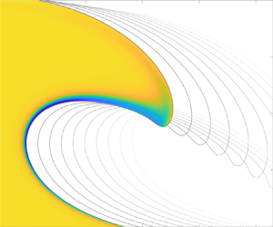
Wave breaking is among the most common and probably most beautiful fluid flows occurring in nature. Yet, it remains extremely challenging to study from a modelling point of view. Being a strongly nonlinear phenomenon, the usual analytical methods fail to capture the full mechanisms. Also, the different scales involved, as well as the free-surface flow, significantly complicate any numerical approach. Our purpose is to provide a new framework to compute numerical viscous water waves, allowing the free surface to overturn until the point at which the interface intersects itself.
Remarkably, the inviscid water wave problem can be reformulated using quantities defined on the water–air interface only (Zakharov Reference Zakharov1968). Several numerical developments are based on such approaches (Longuet-Higgins & Cokelet Reference Longuet-Higgins and Cokelet1976; Vinje & Brevig Reference Vinje and Brevig1981; Baker, Meiron & Orszag Reference Baker, Meiron and Orszag1982; New & Peregrine Reference New and Peregrine1985; Baker & Xie Reference Baker and Xie2011). Even though a complete mathematical description of breaking waves seems unlikely, thorough partial analytical studies have highlighted the possibility of self-similar solutions of a hyperbolic crest leading to a singularity (Longuet-Higgins Reference Longuet-Higgins1982; New Reference New1983).
An alternative route to study the wave breaking phenomenon consists in considering the free-surface Navier–Stokes equations with a small, but finite, viscosity (Chen et al. Reference Chen, Kharif, Zaleski and Li1999; Raval, Wen & Smith Reference Raval, Wen and Smith2009; Di Giorgio, Pirozzoli & Iafrati Reference Di Giorgio, Pirozzoli and Iafrati2022; Mostert, Popinet & Deike Reference Mostert, Popinet and Deike2022). Various instabilities, including the formation of aerated vortex filaments after the breaking stage, could thus be described (Lubin & Glockner Reference Lubin and Glockner2015; Lubin et al. Reference Lubin, Kimmoun, Véron and Glockner2019). The difficulty then lies in approaching the relevant limit of vanishing viscosity and surface tension (when it is included). Surprisingly, none of the recent studies encompassing the viscosity has compared their results with the inviscid case.
Here we introduce a finite-element formulation for the free-surface Navier–Stokes flow and investigate a plunging breaker case. We investigate the formation of a sharp tip on the plunging breaker. We achieve convergence to the Euler solution (Dormy & Lacave Reference Dormy and Lacave2024) and study the role of the viscous boundary layer in regularising the interface.
2. Mathematical formulation
We consider the two-dimensional water domain  $\varOmega _t$ depicted in figure 1, which we assume to be $L$-periodic in $x$. Along the $y$ direction, $\varOmega _t$ is encapsulated between a rigid bottom $\varGamma _b$ of the fluid domain and the water–air interface $\varGamma _{s,t}$, represented by a time-dependent parametrised curve $\boldsymbol {\gamma }_t$. The former will remain unchanged throughout the study whereas the latter is evolving with time. Non-dimensional quantities are defined using the height of fluid at rest $h_0$ as the unit of length, $\sqrt {gh_0}$ as the unit of velocity ( $g$ being the gravitational acceleration), and $\rho g h_0$ as the unit of pressure ( $\rho$ being the fluid density, assumed to be homogeneous). The Reynolds number is then defined as $Re = {\rho h_0 \sqrt {gh_0}}/{\mu }$, where $\mu$ is the fluid dynamic viscosity, also assumed to be homogeneous. Some earlier studies, e.g. Chen et al. (Reference Chen, Kharif, Zaleski and Li1999), Iafrati (Reference Iafrati2009), Deike, Popinet & Melville (Reference Deike, Popinet and Melville2015), Di Giorgio et al. (Reference Di Giorgio, Pirozzoli and Iafrati2022) and Mostert et al. (Reference Mostert, Popinet and Deike2022), used the deep-water scaling to define their Reynolds number, $Re_{{dw}} = \rho \sqrt {g\lambda ^3}/\mu$, where $\lambda$ is the wavelength of the initial wave, here set to $L$, thus $Re_{{dw}}=(L/h_0)^{3/2}Re$.
Geometry of the initial ( $t=0$) domain for the viscous water wave problem.

The incompressible Navier–Stokes equations in the domain  $\varOmega _t$ then take the form
 \begin{equation} \left.\begin{array}{ll@{}} \dfrac{\partial\boldsymbol{u}}{\partial t} + (\boldsymbol{u}\boldsymbol{\cdot}\boldsymbol{\nabla})\boldsymbol{u} +\boldsymbol{\nabla} p - {Re}^{{-}1}\boldsymbol{\nabla}^2\boldsymbol{u} ={-}\hat{\boldsymbol{y}} & \mathrm{in}\ (0,T)\times\varOmega_t,\\ \boldsymbol{\nabla}\boldsymbol{\cdot}\boldsymbol{u} = 0 & \mathrm{in}\ (0,T)\times\varOmega_t,\\ \boldsymbol{u}\boldsymbol{\cdot}\hat{\boldsymbol{n}} = 0 & \mathrm{on}\ (0,T)\times\varGamma_b,\\ \hat{\boldsymbol{t}}\boldsymbol{\cdot}\boldsymbol{\mathsf{S}}\boldsymbol{\cdot}\hat{\boldsymbol{n}} = 0 & \mathrm{on}\ (0,T)\times\varGamma_b,\\ -p\hat{\boldsymbol{n}} + {2}{Re}^{{-}1}\boldsymbol{\mathsf{S}}\boldsymbol{\cdot}\hat{\boldsymbol{n}} = {\kappa{{Bo}^{{-}1}}\hat{\boldsymbol{n}}} & \mathrm{on}\ (0,T)\times\varGamma_{s,t},\\ \boldsymbol{u}(0,\cdot) = \boldsymbol{u}_0 & \mathrm{in}\ \varOmega_0. \end{array}\right\} \end{equation}
Stress-free boundary conditions are imposed at the water–air interface  $\varGamma _{s,t}$, where $\kappa$ is the surface curvature and $Bo^{-1} = \sigma / \rho g h_0^2$ is the Bond number (with $\sigma$ the surface tension). At the bottom $\varGamma _{b}$, we use stress-free conditions in the tangential ( $\hat {\boldsymbol {t}}$) direction and enforce no penetration in the normal direction. The above formulation is sometimes referred to as ‘single fluid’ as the air density has been dropped. Finally, $\boldsymbol{\mathsf{S}}$ denotes the stress tensor defined as $\boldsymbol{\mathsf{S}}(\boldsymbol {u}) = \frac {1}{2}( \boldsymbol {\nabla } \boldsymbol {u} + ( \boldsymbol {\nabla } \boldsymbol {u} )^{\rm T})$.
The interface  $\varGamma _{s,t}$ being a material surface, a two-dimensional advection problem needs to be solved to follow the evolution of $\boldsymbol {\gamma }_t$ with time,
 \begin{equation} \frac{\partial\boldsymbol{\gamma}_t}{\partial t} = \boldsymbol{u}(t,\boldsymbol{\gamma}_t). \end{equation}
With this approach the shape of the interface does not need to be a graph. This is a key property to describe breaking waves and causes difficulties with several formulations of the water-wave problem (see Lannes Reference Lannes2013, chapter 1).
We consider as initial condition a simple wave (solution of the linearised equations) of finite amplitude  $a$ so that the initial interface can be represented as
 \begin{equation} \varGamma_{s,t=0} = \{(x,h_0 + a\cos(kx)),\ \text{with } x\in [0,L]\}, \end{equation}
where  $k = 2{\rm \pi} /L$ denotes the wavenumber. The initial velocity $\boldsymbol {u}_0$ on the interface $\varGamma _{s,t=0}$ is given by a finite-amplitude extension of the first-order two-dimensional solution of the inviscid water wave problem (e.g. Johnson Reference Johnson1997, chapter 2),
 \begin{equation} \boldsymbol{u}_0(x)= a\sqrt{gk\tanh(kh_0)} \cdot \begin{bmatrix} (\tanh (kh_0))^{{-}1}\cos (kx)\\ \sin (kx) \end{bmatrix}. \end{equation}
The initial velocity  $\boldsymbol {u}(0,\cdot )$ in the full fluid domain could be approximated from the series expansion in $ka$. However, since we consider a large-amplitude wave, we would rather compute it numerically. This is easily achieved by solving the Laplace equation for the initial velocity potential $\phi _0$ in $\varOmega _{t=0}$ (hence assuming a vanishing initial vorticity)
 \begin{equation} {\rm \Delta}\phi_0 = 0\ \mathrm{in}\ \varOmega_{0} \quad\text{so that}\quad \boldsymbol{u}(t=0,\boldsymbol{x}) = \boldsymbol{\nabla}\phi_0(\boldsymbol{x}), \end{equation}
with boundary conditions
 \begin{equation} \frac{\partial\phi_0}{\partial\hat{\boldsymbol{n}}} = 0\text{ on }\varGamma_b\quad\text{and}\quad \frac{\partial\phi_0}{\partial\hat{\boldsymbol{n}}} = \boldsymbol{u}_{0}\boldsymbol{\cdot}\hat{\boldsymbol{n}}\text{ on }\varGamma_{s,t=0}, \end{equation}
corresponding to  $\boldsymbol {u}(0,\cdot )\boldsymbol {\cdot }\hat {\boldsymbol {n}} = 0$ on $\varGamma _b$ and $\boldsymbol {u}(0,\cdot)\boldsymbol {\cdot}\hat {\boldsymbol {n}} = \boldsymbol {u}_{0}\boldsymbol {\cdot} \hat {\boldsymbol {n}}$ on $\varGamma _{s,t=0}$.
In order to achieve a finite-element formulation, we need to rewrite problem (2.1) in a weak form. This is achieved by introducing the function space
 \begin{equation} \boldsymbol{H}^1_{\varGamma_b}(\varOmega_t) = \{\boldsymbol{v}\in (H^1(\varOmega_t))^2\text{ such that } \boldsymbol{v}\boldsymbol{\cdot}\hat{\boldsymbol{n}} = 0 \text{ on } \varGamma_b\}, \end{equation}
where  $H^1(\varOmega _t)$ stands for the usual Sobolev space. We then multiply the velocity equation by an arbitrary test function $\boldsymbol {v}\in \boldsymbol {H}^1_{\varGamma _b}(\varOmega _t)$ and the incompressibility condition by another test function $q\in L^2(\varOmega _t)$. Integrating over the whole domain $\varOmega _t$ and making use of our boundary conditions (e.g. Guermond et al. Reference Guermond, Léorat, Luddens and Nore2012) leads to the following variational formulation: Find $\boldsymbol {u}\in \mathcal {C}^1([0,T);\boldsymbol {H}^1_{\varGamma _b}(\varOmega _t))$ and $p\in L^{\infty }([0,T);L^2(\varOmega _t))$ such that
 \begin{align} & \int_{\varOmega_t} \left[\boldsymbol{v}\boldsymbol{\cdot} \frac{\partial\boldsymbol{u}}{\partial t} + \boldsymbol{v}\boldsymbol{\cdot}(\boldsymbol{u} \boldsymbol{\cdot}\boldsymbol{\nabla})\boldsymbol{u}\right. \nonumber\\ &\qquad \left.\vphantom{\frac{\partial\boldsymbol{u}}{\partial t}} +{2}{Re}^{{-}1}\boldsymbol{\mathsf{S}}(\boldsymbol{v})\boldsymbol{:} \boldsymbol{\mathsf{S}}(\boldsymbol{u}) - p\boldsymbol{\nabla}\boldsymbol{\cdot}\boldsymbol{v} - q\boldsymbol{\nabla}\boldsymbol{\cdot}\boldsymbol{u} - \boldsymbol{v}\boldsymbol{\cdot}\boldsymbol{g}\right]{\rm d}^2\boldsymbol{x} \nonumber\\ &\quad =\int_{\varGamma_{s,t}} {\kappa}{Bo^{{-}1}} \boldsymbol{v}\boldsymbol{\cdot}\hat{\boldsymbol{n}} \,{\rm d} S \end{align}
and  $\boldsymbol {u}(0,\cdot) = \boldsymbol {u}_0$ for all test functions $\boldsymbol {v}\in \boldsymbol {H}^1_{\varGamma _b}(\varOmega _t)$ and $q\in L^2(\varOmega _t)$.
3. Numerical discretisation
We numerically approximate solutions of system (2.8) using the FreeFEM language (Hecht Reference Hecht2012).
Once (2.8) has been numerically integrated, the interface must be advected following (2.2). This is achieved using an arbitrary Lagrangian Eulerian method (Hirt, Amsden & Cook Reference Hirt, Amsden and Cook1974). At each iteration, we numerically construct a mesh velocity solving
 \begin{equation} \left.\begin{array}{@{}ll@{}} {\rm \Delta} \boldsymbol{w} = 0 & \text{in}\ \mathcal{T}_h^n,\\ \boldsymbol{w} = 0 & \text{on}\ \varGamma_{b,h},\\ \boldsymbol{w} = \boldsymbol{u}(t,\cdot) & \text{on}\ \varGamma_{s,t_n,h}, \end{array}\right\} \end{equation}
where the subscript  $h$ denotes the discrete numerical boundary. We then advect the mesh vertices using the mesh velocity $\boldsymbol w$. It is thus necessary, in this approach, to recompute finite-element matrices at each time step since the mesh is advected (the Jacobian of the transformation between the reference element and the global cell is thus not constant). The $\boldsymbol {w}$ field is subtracted from the advection term of the fluid equation.
Even though the effects of surface tension are discarded in this study, the capillary term in (2.8) can easily be included in the numerical scheme. Extension to two-phase flows can be considered, at the cost of meshing both domains.
Extension of this approach to the three-dimensional case, though not impossible in theory, will be very challenging in practice. First, this is because of remeshing issues in three dimensions, but also because the number of degrees of freedom needed to achieve convergence to such large Reynolds numbers would then become difficult to handle, even with modern supercomputers. This is due to the need for recomputing matrices at each time iteration with a moving fluid domain. Besides, a major limitation of our approach lies in the impossibility for the interface to intersect itself. Hence the simulation has to stop as soon as a splash has occurred. Analysis of the post-breaking behaviour is not permitted with our approach, but see e.g. Iafrati (Reference Iafrati2009), Deike et al. (Reference Deike, Popinet and Melville2015), Lubin & Glockner (Reference Lubin and Glockner2015), Deike, Melville & Popinet (Reference Deike, Melville and Popinet2016) and Lubin et al. (Reference Lubin, Kimmoun, Véron and Glockner2019).
4. The effect of viscous dissipation on the interface evolution
We consider numerically a domain  $\varOmega _{t=0}$ with $L = 2{\rm \pi}$, $h_0 = 1$ and $a = 0.5$. Surface tension is neglected $\sigma =0$ (thus $Bo^{-1}=0$) in the following. The domain $\varOmega _t$ has been discretised with up to 4000 vertices on the water–air interface. This results in roughly 270 000 triangles and hence about $1.2$ million unknowns for the Navier–Stokes problem.
Simulations were run with Reynolds number ranging from  $10^2$ to $10^6$. Results for $Re = 10^6$ are presented in figure 2, and a comparison of the interface for various Reynolds numbers is available in figure 3. The resulting wave behaves as a plunging breaker – see the classification of Galvin (Reference Galvin1968). We should stress that the initial condition being irrotational, the vorticity vanishes everywhere except for a thin boundary layer near the surface (see § 5). The fact that the vorticity is localised helps in the numerical resolution at large values of the Reynolds number.
Evolution of the interface with time at  $Re = 10^6$. (An animation corresponding to the simulation presented in this figure is available as supplementary material available at https://doi.org/10.1017/jfm.2024.208.)

Interface evolution with time for different values of the Reynolds number with emphasis on the tip of the wave. The Euler solution was obtained from Dormy & Lacave (Reference Dormy and Lacave2024). The shaded region corresponds to the Euler fluid domain.

Our objective is now to characterise the convergence as the Reynolds number is increased. The time evolution of the interface is compared for different Reynolds numbers with the same initial condition in figure 3. The solution of the Euler equation (Dormy & Lacave Reference Dormy and Lacave2024) for the same problem is also included for comparison. The regularising effects of dissipation are clearly visible. The overhanging region takes a round shape and falls faster at larger dissipation (i.e. for decreasing Reynolds number). Perhaps more surprisingly, the effects of dissipation are localised near the plunging jet. The Euler interface appears to provide a limit solution towards which the Navier–Stokes solution converges as the Reynolds number is increased. Only a very small difference remains between the Euler solution and the Navier–Stokes solution for  $Re = 10^6$. This minute difference may be due to the finiteness of $Re$ but also possibly to some amount of numerical diffusion, as this extreme Reynolds number case is at the edge of our numerical resolution (see below).
In order to quantify the convergence of the finite-Reynolds-number flow to the Euler solution, we must measure the differences between the various interface positions. (The numerical convergence at a given  $Re$ was assessed varying the mesh size (see the Appendix).) We cannot use a standard norm to do that, since the interface is not a graph as soon as the wave overturns. We therefore rely (as in Dormy & Lacave Reference Dormy and Lacave2024) on the bidirectional Hausdorff distance between the curves, i.e.
 \begin{equation} \delta_H(A,B)=\max(\tilde{\delta}_H (A,B),\tilde{\delta}_H(B,A)),\quad \text{with}\ \tilde{\delta}_H(A,B)=\max_{a\in A} \min_{b\in B} \| a-b \|. \end{equation}
The time evolution of the distance between each curve obtained for a given Reynolds number and the Euler solution is presented in figure 4(a). The initial condition being identical, the distance is a growing function of time until the splash approaches. The time at which the effect of viscosity becomes significant increases as the Reynolds number increases.
(a) Convergence of the Navier–Stokes solutions to the Euler solution (Dormy & Lacave Reference Dormy and Lacave2024) as the Reynolds number is increased using the Hausdorff distance. (b) Time evolution of the maximum curvature radius with time for different values of the Reynolds number. The last four curves are indistinguishable at this scale.

No finite-time wedge-like singularity seems to be developing for the initial condition considered here, even in the case of the Euler solution (Dormy & Lacave Reference Dormy and Lacave2024). This can be assessed by introducing the minimum curvature radius  $R_c(t)$ (see figure 4b). The curvature of the interface can be computed numerically, with a maximum corresponding to the crest. The minimum curvature radius $R_c(t)$ is then the inverse of the maximum curvature. Figure 4(b) presents $R_c$ as a function of time. Each simulation is interrupted when the interface self-intersects. Though $R_c$ tends to zero for large enough Reynolds number, it remains strictly positive for all time in all our simulations. No finite-time singularity is obtained for this set-up. Our low-Reynolds-number cases $Re \leq 10^3$ are characterised by a larger $R_c(t)$. The fact that the curves are indistinguishable in the figure for $Re \geq 10^4$, and coincide with the Euler simulation of Dormy & Lacave (Reference Dormy and Lacave2024), indicate that the lack of finite-time singularity for this configuration is not a consequence of viscosity and that the Bernoulli principle, accelerating the fluid near the tip of the wave (Pomeau & Le Berre Reference Pomeau and Le Berre2012), does not cause a singularity for such initial data. Further initial conditions and domain geometries thus need to be investigated to study the necessary conditions for the formation of such a singularity.
5. Energy dissipation
To further characterise the difference between the Euler and Navier–Stokes solutions, we now investigate the spatial distribution of viscous dissipation. A typical global energy-balance equation can be computed by setting  $\boldsymbol {v} = \boldsymbol {u}$ in the weak formulation (2.8) and using the incompressibility condition,
 \begin{align} \frac{{\rm d}}{{\rm d} t}\int_{\varOmega_t} \frac{\boldsymbol{u}^2}{2}\,{\rm d}\kern0.06em \boldsymbol{x} &= \int_{\varOmega_t} \left(\boldsymbol{g} \boldsymbol{\cdot} \boldsymbol{u} - \frac{2}{Re} \boldsymbol{\mathsf{S}}(\boldsymbol{u})\boldsymbol{:} \boldsymbol{\mathsf{S}}(\boldsymbol{u})\right)\,{\rm d}\kern0.06em \boldsymbol{x} \nonumber\\ &={-}\frac{1}{2}\frac{{\rm d}}{{\rm d} t}\int_{\varGamma_{s,t}} y^2n_y\,{\rm d} S - \frac{2}{Re} \int_{\varOmega_t} \boldsymbol{\mathsf{S}}(\boldsymbol{u})\boldsymbol{:} \boldsymbol{\mathsf{S}}(\boldsymbol{u})\,{\rm d}\kern0.06em \boldsymbol{x}, \end{align}
for a vertical gravitational acceleration  $\boldsymbol {g} = -\hat {\boldsymbol {y}}$ and a flat bottom. This is the usual kinetic and potential energy for water waves (e.g. Lannes Reference Lannes2013) with an additional viscous dissipation term.
A local equation for the kinetic energy can also be computed directly by multiplying the Navier–Stokes equation (2.1) by  $\boldsymbol {u}$ and using the typical relation ${\rm \Delta} \boldsymbol {u} = -\boldsymbol {\nabla }^\perp (\boldsymbol {\nabla }^\perp \boldsymbol {\cdot}\boldsymbol {u}) = -\boldsymbol {\nabla }^\perp \omega$, where $\boldsymbol {u}^\perp = (-u_y,u_x)$ denotes a ${{\rm \pi} }/{2}$ anticlockwise rotation and $\omega = \boldsymbol {\nabla }^\perp \boldsymbol {\cdot} \boldsymbol {u}$ is the two-dimensional vorticity. This leads to
 \begin{equation} \frac{{\rm d}}{{\rm d} t}\frac{\boldsymbol{u}^2}{2} = \boldsymbol{g}\boldsymbol{\cdot}\boldsymbol{u} - \boldsymbol{u}\boldsymbol{\cdot}\boldsymbol{\nabla} p + \frac{1}{Re}[\boldsymbol{\nabla}\boldsymbol{\cdot}(\boldsymbol{u}^\perp\omega)-\omega^2]. \end{equation}
Hence the viscous dissipation happens in regions of the domains where the vorticity does not vanish.
The vorticity is represented in figure 5(a–e). Note the formation of a vorticity sheet near the interface as the Reynolds number is increased. The Lundgren & Koumoutsakos (Reference Lundgren and Koumoutsakos1999) theorem states that the source of mean vorticity in the boundary layer is in fact this superficial vortex sheet. It is interesting to note that a small-magnitude positive-vorticity boundary layer appears at the tip of the wave (see figure 5f). As time proceeds, the vorticity sheet grows where the curvature of the interface becomes important – see Longuet-Higgins (Reference Longuet-Higgins1992), for the steady-state case.
(a–e) Vorticity  $\omega$ near the tip of the wave for different values of the Reynolds number at time $t = 2.9$. (f) A zoom on the tip of the wave for the $Re = 10^5$ case. The colour legend has been truncated from below to guarantee overall colour coherence.

The boundary layer is expected to scale as  $Re^{-1/2}$ – see e.g. Landau & Lifshitz (Reference Landau and Lifshitz1987) for the general theory, Liu & Davie (Reference Liu and Davie1977) for the particular case of viscous water waves and Masmoudi & Rousset (Reference Masmoudi and Rousset2017) for a mathematical description of this limit. We present in figure 6 vorticity cross-sections in the normal direction starting on the interface at $y=0.925$ (indicated on figure 5a–e). The boundary layer of the $Re = 10^6$ case is spread over three to four nodes at most, so that the exponential behaviour is not clearly captured. Figure 6 nevertheless clearly illustrates the $Re^{-{1}/{2}}$ scaling of the boundary layer for $Re = 10^3$ to $Re = 10^5$ and is compatible with the scaling for $Re = 10^6$. As already mentioned, the $Re = 10^2$ case is so viscous that the interface does not exhibit the same characteristics as the others. The inward-pointing normal vector at $y=0.925$ is ascending whereas the others are descending. This explains the different behaviour in figure 6.
Vorticity cross-sections along the straight lines, normal to the boundary, shown in figure 5(a–e). Here  $s$ is the arclength, which parametrises the lines.

Interestingly the vorticity sheet becomes comparable in size to the minimum curvature radius  $R_c$ near $Re = 10^4$, i.e. when the curvature radius, as a function of the Reynolds number, reaches its minimum (figure 4). Another striking aspect of figure 6 lies in the value of the vorticity at the boundary, which appears to be fairly independent of the Reynolds number. This suggests a pointwise convergence to the interface vorticity of the Euler problem, i.e. the vortex intensity $\gamma$ in Baker et al. (Reference Baker, Meiron and Orszag1982).
6. The regularising effects of viscosity
The formation of a vorticity layer near the interface is associated with the viscous regularisation of the boundary. Indeed, following Longuet-Higgins (Reference Longuet-Higgins1953) we can define a curvilinear coordinate system  $(s,n)$ following the interface with time. This coordinate system is sometimes known as the Frenet frame. Here $s$ denotes the arclength while $n$ is the normal coordinate, pointing inwards (figure 7a). We also write $\boldsymbol {u} = u_s\hat {\boldsymbol {s}} + u_n\hat {\boldsymbol {n}}$, i.e. the decomposition of the fluid velocity along the tangential and normal vectors. The time evolution of the curvature $\kappa$ (positive when convex inwards) of the interface can be expressed as
 \begin{equation} \frac{\partial\kappa}{\partial t} = \frac{\partial^2 u_n}{\partial s ^2} - u_s\frac{\partial \kappa}{\partial s} + \kappa^2u_n, \end{equation}
where  $u_s$ and $u_n$ are evaluated at $n=0$. The full argument can be found in Longuet-Higgins (Reference Longuet-Higgins1953, § 6), with a different sign convention for the curvature.
Coordinate system  $(s,n)$ definition, and geometrical interpretation of $h$ and $\kappa$.

Defining the metric factor  $h = 1 - n\kappa (t,s)$ (see figure 7), the continuity equation becomes
 \begin{equation} \boldsymbol{\nabla}\boldsymbol{\cdot}\boldsymbol{u} = \frac{\partial u_s}{\partial s} + \frac{\partial }{\partial n}(hu_n) = 0. \end{equation}
The full Navier–Stokes equations written in such a coordinate system can be found in Longuet-Higgins (Reference Longuet-Higgins1953). We introduce the streamfunction  $\psi$ such that
 \begin{equation} u_s = \frac{\partial \psi}{\partial n} \quad\text{and}\quad u_n ={-} \frac{1}{h}\frac{\partial \psi}{\partial s}. \end{equation}
The vorticity is defined as
 \begin{equation} \omega = h^{{-}1}\left( \frac{\partial u_n}{\partial s} - \frac{\partial }{\partial n}(hu_s)\right). \end{equation}
Where the vorticity vanishes, we can define a velocity potential  $\phi$ as
 \begin{equation} u_s = \frac{1}{h}\frac{\partial \phi}{\partial s}\quad\text{and}\quad u_n = \frac{\partial \phi}{\partial n}. \end{equation}
Inserting  $\phi$ and $\psi$ in the continuity equation (6.2) and vorticity equation (6.4) yields
 \begin{equation} {\rm \Delta}\phi = 0 \quad\text{and}\quad {\rm \Delta}\psi ={-}\omega. \end{equation}
We now decompose the flow as a global potential plus a local viscous component (e.g. Lundgren & Koumoutsakos Reference Lundgren and Koumoutsakos1999),  $\boldsymbol {u} = \boldsymbol {\nabla }\phi + \boldsymbol {\nabla }^\perp \psi _{Re},$ where $\boldsymbol {\nabla }^\perp$ is defined by (6.3a,b). The $\psi _{Re}$ component, i.e. viscous effects, localised in a boundary layer of size $\delta = Re^{-({1}/{2})}$, disappear as the viscosity vanishes (see figure 5). We introduce an expansion of $\psi _{Re}$ in powers of $\delta$,
 \begin{equation} \psi_{Re}(s,n,t) = \delta\psi_1(s,n,t) + \delta^2\psi_2(s,n,t) + O(\delta^3). \end{equation}
Furthermore, because of the boundary layer structure, we can introduce  $\varPsi _{Re}(s,{n}/{\delta },t) \equiv$ $\psi _{Re}(s,n,t)$. Inserting the expression (6.7) into the vorticity equation (6.4) leads to terms of order $O(\delta ^{-1})$. Figures 5 and 6, however, highlight that the vorticity remains of order $O(1)$, leading to the conclusion that $\psi = O(\delta ^2)$ and hence that $\psi _1 = 0$.
Rewriting the curvature evolution equation (6.1) with  $\phi$ and $\varPsi _{Re}$, we find that
 \begin{align} \frac{\partial \kappa}{\partial t} &= \frac{\partial^3\phi}{\partial n \partial^2s} - \frac{1}{h} \frac{\partial \phi}{\partial s}\frac{\partial \kappa}{\partial s} + \kappa^2 \frac{\partial \phi}{\partial s} \nonumber\\ &\quad +\underbrace{\frac{\partial^2 }{\partial s ^2}\left( \frac{1}{h}\frac{\partial \psi_{Re}}{\partial s} \right)}_{O(\delta^2)} - \underbrace{\frac{\partial \kappa}{\partial s}\frac{\partial \psi_{Re}}{\partial n}}_{O(\delta)} + \underbrace{\frac{\kappa^2}{h}\frac{\partial \psi_{Re}}{\partial s}}_{O(\delta^2)}. \end{align}
The effects of viscous dissipation on the interface thus enter the leading-order balance when the surface curvature becomes of order  $O(\delta ^{-1})$ (i.e. a curvature radius of order $O(\delta )$). Conversely, when the surface curvature becomes of order $O(\delta )$ or smaller, viscous effects appear in time $O(\delta ^{-2})$. In practice, for the large Reynolds numbers applicable to water waves, surface tension will also become significant at similar scales.
7. Conclusions
The present work has demonstrated that the viscous water wave problem converges towards the inviscid solution, even in the case of wave breaking. We highlighted the regularising effect of finite viscosity and quantified the curvature at which viscous effects become significant. Further work, involving different initial conditions, is needed regarding the possible formation of a finite-time singularity at the tip of a breaking wave.
Supplementary material
A supplementary animation corresponding to the simulation in figure 2 is available at https://doi.org/10.1017/jfm.2024.208.
Acknowledgements
The authors wish to acknowledge discussions with C. Lacave on water waves, and with B. Maury and P. Jolivet on the use of FreeFEM.
Declaration of interests
The authors report no conflict of interest.
Appendix. Numerical convergence
All simulations have been carried out with meshes of different sizes, measured by  $N$, the number of points at the free surface. (The total number of degrees of freedom of the finite-element mesh is much larger than $N$. For example for $Re = 10^6$ with $N=4000$, the final number of degrees of freedom is $\simeq 2.2 \times 10^6$.) Different values of $N$ have been used depending on the Reynolds number. Numerical convergence is highlighted in figure 8 by using in each case grids with $N/2$, $N/4$ and $N/8$ points at the free surface.
Numerical convergence for each Reynolds number; the rectangular region indicated on the left is blown up on the right. Note that  $N=1000$ for $Re = 10^6$ is unstable for times larger than $2.2$, thus only two meshes are compared in the last graph.


 Open access

