

INTRODUCTION
The functioning of river catchments is the crucial indicator of climate variability and environmental changes occurring in the Arctic. Understanding the determinants of the processes taking place under the influence of changing elements of the water cycle requires identification of the spatial dynamics of the snow cover disappearance, rainfall and changes of runoff in summer season. The derivation of relationships between meteorological conditions over a catchment area and the resulting outflow in a stream is a fundamental problem. Higher air temperatures and the increased precipitation observed in Svalbard in the last two decades lead to prolongation of the ablation season (Osuch and Wawrzyniak, Reference Osuch and Wawrzyniak2016b). Future changes in the length of ablation season, precipitation and river outflows can alter fluxes of fresh water, sediments and nutrients. This would have implications for aquatic ecosystems (Blaen and others, Reference Blaen, Hannah, Brown and Milner2014; Osuch and Wawrzyniak, Reference Osuch and Wawrzyniak2016a).
For decades, ongoing international research activities aimed at improving knowledge and understanding of the processes involved. Hydrological recognition of the Arctic region still remains far less developed than it is at lower latitudes. Limited data availability is mainly due to extreme weather conditions and difficult accessibility (Sund, Reference Sund2008). Hydrological modelling studies for Arctic catchments are not common. The published studies include an application of different hydrological models. Among them three-dimensional coupled MIKE SHE-MIKE 11 model was used for the ice-free Two Boat Lake catchment, Western Greenland (Johansson and others, Reference Johansson2015); CPIsnow model for 12 boreal catchments located in Northern Finland (Akanegbu and others, Reference Akanegbu, Marttila, Ronkanen and Kløve2017); and WATCLASS used to simulate spring snowmelt run-off in a Trail Valley Creek in Canada (Pohl and others, Reference Pohl, Davison, Marsh and Pietroniro2005). The research efforts carried out in previous years in Svalbard were focused primarily on glaciated catchments, including Bayelva (Hodgkins, Reference Hodgkins1997; Sund, Reference Sund2008), Ebbaelva (Rachlewicz, Reference Rachlewicz2009; Dragon and others, Reference Dragon, Marciniak, Szpikowski, Szpikowska and Wawrzyniak2015), Scottelva (Franczak and others, Reference Franczak, Kociuba and Gajek2016), Waldemarelva (Sobota, Reference Sobota2014), and Breelva (Majchrowska and others, Reference Majchrowska, Ignatiuk, Jania, Marszałek and Wąsik2015). Nowak and Sobota (Reference Nowak and Sobota2015) used artificial neural networks for glaciated Waldemar catchment. The Deterministic Modelling Hydrological System (DMHS) helped to complete missing hydrological data for Werenskiöld glacier catchment (Majchrowska and others, Reference Majchrowska, Ignatiuk, Jania, Marszałek and Wąsik2015).
In this paper, the conceptual catchment run-off HBV (Hydrologiska Byråns Vattenbalansavdelning) model (Bergström, Reference Bergström and Singh1995) was applied to describe small non-glaciated Arctic catchments, specifically Fuglebekken. This hydrological model introduced by Swedish Meteorological and Hydrological Institute (Bergström and Forsman, Reference Bergström and Forsman1973; Bergström and Lindström, Reference Bergström and Lindström2015) is currently well recognized and widely used for an increasing number of applications and purposes. The HBV model was used for the first time in Svalbard in 1991 for the Bayelva catchment (Bruland, Reference Bruland1991). It was also applied for modelling of outflows of Endalen/Isdammen, de Geerelva and Bayelva (Bruland and Killingtveit, Reference Bruland and Killingtveit2002).
The Fuglebekken catchment well represents the areas of sea terraces and coastal mountains without glaciers that are quite common along the western coast of Spitsbergen. Recent expansion of the ice-free areas is observed, so the recognition of the functioning of river ecosystems and the supply of fresh water to the surrounding fjords and seas becomes more and more essential (Błaszczyk and others, Reference Błaszczyk, Jania and Hagen2009). Discharge measurements from Fuglebekken catchment were carried out in previous years: 1979/80 (Pulina and others, Reference Pulina, Krawczyk and Pereyma1984), and partly from 1988 to 1992 (Jania and Pulina, Reference Jania, Pulina, Sand and Killingtveit1994). However, these measurements were not made on regular basis. For the first time, discharge was measured at 10 min interval throughout most of the summer seasons of 2014 and 2015. High temporal resolution of relevant observations made the first attempt to model the catchment runoff possible. The applied HBV model has a structure with five conceptual storages taking into account dominant processes in the catchment: snow accumulation and melting, soil moisture, fast and slow runoff. The appropriate description of those processes and their simulations results at small catchment scale requires the input of hydro-meteorological data at appropriate temporal scale. The time required for runoff to travel from the hydraulically most distant point to the outlet or gauging station is described by the time of concentration (TC). It is a primary parameter recommended in hydrological modelling that should guarantee appropriate description of the dynamics of the catchment and an adequate accuracy of simulation results. TC can be computed using many different methods and depends on the stream slope, length of the channel and other morphometric properties of the catchment. An estimate of TC by the Kirpich formula (Kirpich, Reference Kirpich1940) for the Fuglebekken catchment is slightly longer than 10 min. Therefore, at least the same temporal resolution is required for catchment run-off modelling. Unfortunately, the estimates of TC are uncertain and the differences in the TC values calculated with different methods can reach up to 500% (Grimaldi and others, Reference Grimaldi, Petroselli, Tauro and Porfiri2012). This raises the issue of the appropriate time step of data used as input to hydrological models.
This paper aims to analyze the influence of data time step on the calibration and validation results of the HBV model as well as on the values of parameters. The studies by Littlewood and Croke (Reference Littlewood and Croke2008), Bastola and Murphy (Reference Bastola and Murphy2013), Wang and others (Reference Wang, Li and Hao2015) revealed that the time step influences the model performance as well as model parameters. An influence of input data averaging on the discharge modelling results was also investigated. This type of hydrological modelling requires input data (precipitation, air temperature, potential evapotranspiration (PET)) and discharge values at an appropriate time step. Generally, a series of averages or sums over a time period should be applied, but due to limited observations, instantaneous and averaged values of discharges, as well as air temperature and the PET, are used in this study. As it is presented, the choice of instantaneous versus averaged data can influence the modelling results.
STUDY AREA
The Fuglebekken catchment is located in the close vicinity of the Polish Polar Station, Hornsund (PPS) (77°00′N 15°30′E), on the northern shore of the Hornsund fjord in southern part of Spitsbergen, the largest island of Svalbard Archipelago (see Fig. 1). Fuglebekken has been a part of many scientific investigations since 1970s for determination of geomorphology (Karczewski and others, Reference Karczewski1990); fluvial processes (Pulina and others, Reference Pulina, Krawczyk and Pereyma1984; Jania and Pulina, Reference Jania, Pulina, Sand and Killingtveit1994); chemical denudation (Krzyszowska, Reference Krzyszowska1985; Kozak and others, Reference Kozak2015; Skrzypek and others, Reference Skrzypek2015); permafrost and active layer thickness (Leszkiewicz and Caputa, Reference Leszkiewicz and Caputa2004; Sobota and Nowak, Reference Sobota and Nowak2014; Wawrzyniak and others, Reference Wawrzyniak, Osuch, Napiórkowski and Westermann2016).
Study area. Changed after Jania and others (Reference Jania, Kolondra and Aas2002).

The catchment up to outflow measurement point covers an area of 1.27 km2. The catchment originates on the southern slopes of the mountain ridge Ariekammen-Fugleberget and elevated marine terraces of abrasion-accumulation plain Fuglebergsletta. Hydrographic cover includes few tributaries of Fuglebekken stream and a small water reservoir of size 0.0048 km2. Despite its small size, the catchment is heterogenous in terms of land cover and topography. The elevations range from 522 m a.s.l. just below the summit of Fugleberget and 513 m a.s.l. of Ariekammen to 4 m a.s.l, where the hydrological profile is located. Below this point, Fuglebekken drains into the Isbjørnhamna bay. The slopes of Fugleberget and Ariekammen are covered with washed rubble sediments, solifluction tongues, rock streams, alluvial cones and bare solid rock of Hecla Hoek geological formation (Czerny and others, Reference Czerny, Kieres, Manecki and Rajchel1993; Harland, Reference Harland1997). Below the slopes, marine terraces covered with sea gravel (elevation from 2 to 30 m a.s.l.), raised during Holocene (Lindner and others, Reference Lindner, Marks, Roszczynko and Semil1991) are covered by a diversity of tundra vegetation types (Migała and others, Reference Migała, Wojtuń, Szymański and Muskała2014), of which 32.5% of the catchment area is covered by Geophytic initial tundra (Skrzypek and others, Reference Skrzypek2015). Close to the eastern boundary of the catchment lies the lateral moraine of Hansbreen glacier, which was at its maximum Holocene extent in Little Ice Age (Błaszczyk and others, Reference Błaszczyk, Jania and Hagen2009). The ground here has a continuous permafrost layer down to more than 100 m depth (Humlum and others, Reference Humlum, Instanes and Sollid2003; Christiansen and others, Reference Christiansen2010; Wawrzyniak and others, Reference Wawrzyniak, Osuch, Napiórkowski and Westermann2016).
Meteorological data have been collected continuously at PPS since July 1978. In the period 1979–2015, the mean annual air temperature at PPS was −3.9°C; the warmest month is usually July, with an average air temperature 4.4°C; the coldest month is March with an average temperature of −10.3°C (Osuch and Wawrzyniak, Reference Osuch and Wawrzyniak2016b). The highest air temperature recorded at PPS reached 15.6°C on the 31 July 2015. The mean annual precipitation was 440 mm. Snow covers the ground on lower elevations ~250 days a−1. Snow cover in this area during spring reaches from 0.30 m on flat surfaces of marine terraces, 0.80 m in upper parts of the slopes, up to 2.00 m at the bottom of the slopes (Winther and others, Reference Winther2003).
HYDRO-METEOROLOGICAL DATA
The flow of water in rivers on Spitsbergen has a seasonal character. During late autumn, winter and early spring, in non-glaciated catchments, rivers freeze. There is a typical large variation of flow of water during ablation season, with very high discharge during the snowmelt and decreases during the summer (Killingtveit and others, Reference Killingtveit, Pettersson and Sand2003). Due to the higher precipitation in late summer and early autumn, higher flow can be observed before the freezing season (Osuch and Wawrzyniak, Reference Osuch and Wawrzyniak2016b).
Comparison of hydro-meteorological data from two consecutive years 2014 and 2015 is presented in Figure 2. Although the time courses of the air temperature look similar in both years with average monthly temperature differences for each July, August and September no higher than 0.1°C, precipitation amounts differ significantly. August 2014 was one of the driest in the history of measurements at PPS with a monthly sum of precipitation reaching 16.6 mm. Rainfall occurred in the end of August after almost a month with only a trace of precipitation. After such long drought, there was almost no catchment response to the precipitation event on the 28 and 30 August.
Air temperature, precipitation and discharge in 10 min interval in 2014 and 2015 at Fuglebekken catchment.

Hydrological investigations were conducted in periods from 14 June to 18 September 2014 and from 21 June to 18 September 2015. The water circulation is influenced by a number of factors that are variable in time. The lengths of the measurement periods were conditioned by river icing. Rivers in this area are frozen and covered with thick snowdrift from October until the end of May. The start of the ablation and the melt rate is governed primarily by the variability of the thermal-radiation factors (Sobota, Reference Sobota2014; Majchrowska and others, Reference Majchrowska, Ignatiuk, Jania, Marszałek and Wąsik2015; Franczak and others, Reference Franczak, Kociuba and Gajek2016). Snow cover and river ice disappearance create disturbances for flow measurements during a brief but intense snowmelt period, so the discharge data since the beginning of July were used. In both years, discharge was measured in the same profile (77.0053°N, 15.5561°E) using portable flowmeter Nivus PCM-F, designed for water level, velocity and flow monitoring in rivers and channels. Active Doppler sensor (KDA-KP 10) uncertainty is ±1% of the final value of velocity and ≤0.5% of final value of the water level. This instrument was installed on the bottom of Fuglebekken stream in the deepest point of the profile.
For the first time in the Hornsund region, the catchment runoff was measured with a 10 min time step. The open channel discharge measurement using the Doppler sensor has many advantages as well as some deficiencies. The portable Nivus PCM-F device is designed to record instantaneous velocity components at a single point with a relatively high frequency. Calculations are performed by measurement data of the velocity of particles in a remote sampling volume based upon the Doppler shift effect above the sensor and then automatically multiplied by the cross-section area. These measurements were carried out in unattended way for the entire ablation period. Data are reliable and accurate. They are comparable with results of velocity area method carried out with Electromagnetic Open Channel Flow Meter Valeport Model 801 with a Flat Type sensor. The velocity measurements were performed several times during each season and results between instruments varied only up to 15%.
The uncertainty of the measurement depends mainly on the channel geometry, which is the same during the entire ablation season. The river close to the gauging point is characterized by relatively low-stream gradient and low-sediment transport, so the channel geometry is almost constant during the season.
For the HBV model setup and calibration, meteorological data were provided by the Institute of Geophysics, Polish Academy of Sciences that manages the PPS. Air temperature and precipitation at 1 min resolution are measured routinely at meteorological site of PPS located ~500 m to the south-west from the outflow measurement point. PET was calculated using temperature-based Hamon method (Hamon, Reference Hamon1961).
METHODS
Catchment run-off models
In this study, a conceptual HBV model was applied, which is a general-purpose hydrological model introduced by Swedish Meteorological and Hydrological Institute (Bergström and Forsman, Reference Bergström and Forsman1973; Bergström and Lindström, Reference Bergström and Lindström2015) and currently available in different forms and versions used for an increasing number of applications and purposes (Bergström, Reference Bergström and Singh1995; Lindström and others, Reference Lindström, Johansson, Persson, Gardelin and Bergström1997; Booij, Reference Booij2005; Booij and Krol, Reference Booij and Krol2010; Romanowicz and others, Reference Romanowicz, Osuch and Grabowiecka2013; Osuch and others, Reference Osuch, Romanowicz and Booij2015; Piotrowski and others, Reference Piotrowski, Napiorkowski, Napiorkowski, Osuch and Kundzewicz2017). Conceptual models have moderate data requirements and their parameters are obtained by calibration and validation. A detailed description of the HBV model version applied in this study is presented by Piotrowski and others (Reference Piotrowski, Napiorkowski, Napiorkowski, Osuch and Kundzewicz2017). As presented in Figure 3, this version includes five conceptual storages as primary hydrological units that take into account the dominant processes in catchment run-off modelling: (a) snowmelting (b) snow accumulation, (c) soil moisture, (d) fast and (e) slow runoff. The input data are precipitation, air temperature and PET. The principal output is discharge; however, the other variables relating to water balance components (evapotranspiration, soil moisture and water storage) are also available from the model.
Structure and parameters of the HBV model.

Similarly to the HBV version used by Piotrowski and others (Reference Piotrowski, Napiorkowski, Napiorkowski, Osuch and Kundzewicz2017), the model has 13 parameters of which values are estimated by calibration with ranges described in Table 1. Five parameters are related to snow processes: TT, TTI, CFMAX, CFR and WHC. Three parameters FC, LP and β are related to the second conceptual storage (soil moisture). CFLUX represents the capillary transport between the fast run-off reservoir and the soil moisture reservoir. KF and α parameters describe the fast runoff. Percolation – the transport between the fast and slow run-off reservoirs – is described by the parameter PERC, while the slow run-off reservoir is represented by the KS parameter.
The HBV model parameters and their ranges used for calibration

The HBV model was originally developed and is usually operated on daily time step data. In small mountainous catchments, such as Fuglebekken, discharge peaks are maintained only for short periods of time, usually lasting less than an hour. Due to that and the aforementioned the time of concentration parameter in this study, discharge data were recorded with 10 min time step.
Initial conditions for soil moisture and other storages were analyzed beforehand and assumed to be the same for both years. As a result of such testing, we excluded first 3 days of simulation from the time series used for calculation of objective function.
The HBV model is an example of conceptual rainfall-run-off hydrological model that was developed using water balance averaged over time steps. In hydrological practice, the model is calibrated using discrete instantaneous flow observations that might be different than the averaged values. As detailed discharge observations were obtained for the Fuglebekken catchment, an influence of input data averaging (discharges, air temperature and PET) on the calibration and validation results was investigated.
Model calibration
Model calibration was carried out using the Differential Evolution with Global and Local neighbours (DEGL), a global optimization method described by Das and others (Reference Das, Abraham, Chakraborty and Konar2009) and Piotrowski and Napiorkowski (Reference Piotrowski and Napiorkowski2012). Following the literature review, the parameters of DEGL method were established (population size N = 5 × M; scale factor F = 0.8; the cross-over rate CR = 0.9). As a stopping criterion, maximum number of iterations were used, namely 30 000. The applied method for parameter optimization provides reliable estimates of model parameters (Piotrowski and others, Reference Piotrowski, Napiorkowski, Napiorkowski, Osuch and Kundzewicz2017); however, in some cases the method suffers of premature convergence to the local optima instead of proceeding to the global optimum (Das and others, Reference Das, Abraham, Chakraborty and Konar2009). To analyze this problem, the DEGL algorithm was run independently 30 times starting from different, randomly generated initial conditions.
As an objective function, the Nash–Sutcliffe coefficient (NS) of efficiency was applied (Nash and Sutcliffe, Reference Nash and Sutcliffe1970). It is defined as:
 $$NS = 1 - \displaystyle{{\sum\nolimits_{t = 1}^n {(Q_{{\rm obs},t} - Q_{\rm m} )^2}} \over {\sum\nolimits_{t = 1}^n {(Q_{{\rm obs},t} - \overline {Q_{{\rm obs}}} )^2}}} $$
where Q
obs is observed discharge, Q
m is modelled values of discharge at time t and $\overline {Q_{{\rm obs}}} $
denotes mean observed discharge.
$\overline {Q_{{\rm obs}}} $
denotes mean observed discharge.
NS values can range from minus infinity (−∞) to 1. A value of 1 corresponds to a perfect match between model and observations.
In this study, the HBV model was calibrated independently for:
-
• two ablation seasons (2014 and 2015);
-
• 11 time steps (10, 20, 30, 40, 60 and 90 min; 2, 3, 6, 12 and 24 h);
-
• discrete (instantaneous) and averaged over time interval data.
In addition, the HBV model was validated for each year (2014, 2015) using the HBV model developed on other year (2015 and 2014, respectively) with the same time step and averaging.
RESULTS
The results of the HBV model calibration for 11 different time steps and for 2 years were analyzed taking into account the effect of time step on model calibration and validation (maximum fit and also spread in the results) and the effect of time step on the values of parameters.
The effect of time step on the model fit
The results of calibration using data from year 2014 and 2015 are presented in the upper row of Figure 4 in the form of boxplots that represent the spread of the NS obtained for 30 runs of calibration procedure. In each boxplot, the bottom and the top of the box represent the first and third quartiles and the red line inside the box represents the median of the calculated model fit (NS values). The error bars represent the minimum and maximum NS from 30 runs of calibration procedure. The applied calibration procedure for each time step resulted in different values of objective function as well as model parameters. It is visible that the values of NS depend on the data time step as well as on the calibration year.
A comparison of the calibration (upper row) and validation (bottom row) results for discrete data from year 2014 (on the left) and 2015 (on the right). Boxplots present the NS obtained for different data time steps. In each boxplot, the bottom and top of the box represent the first and third quartiles and the red line inside the box represents the median. The error bars represent the minimum and maximum from 30 runs of calibration procedure.

In the case of calibration results for year 2014 (upper left panel in Fig. 4), the best match between observations and simulations was obtained for 60 min time step (0.88). The maximum values of NS for time steps 10, 20, 30, 40 and 90 min are > 0.85, just slightly smaller than for 60 min. The results for longer time steps (6, 12 and 24 h) are characterized by lower maximum values of NS (smaller than 0.80) from the sample of calibration runs.
The maximum values of NS obtained at the calibration stage for year 2015 resemble tendencies as for year 2014. In this case, the maximum NS value was obtained for 20 min time step (0.89). In both years, the results for time steps shorter than 6 h are larger than 0.80. The NS values for longer time steps decrease with increasing time step.
The results of validation are presented in the bottom row of Figure 4. The panel on the left shows results of model validation from 2014 on data from 2015, while on the right results of model validation from 2015 on data from 2014. The best results of validation (NS higher than 0.67) were obtained for two time steps (3 and 6 h) for validation of models from 2015 on data from 2014. Good results of validation (NS higher than 0.50) were obtained for time steps from 20 min till 3 h for models from 2014 and from 30 min till 6 h for models from 2015. Negative values of NS were obtained at validation stage for time steps 12 and 24 h for models from 2014. The validation results of models from 2015 for all tested time steps gave positive NS values.
Spread in the model fit (NS values)
A comparison of NS values for 30 runs of calibration and validation are characterized by spread in the obtained results that depend on data time step and also on the year.
The median values of calibration with NS higher than 0.70 were estimated for time steps from 90 min up to 12 h for discharge data from 2014 and from 10 min up to 3 h for 2015. Median values of NS for calibration were higher than 0.81 for time intervals from 10 min up to 2 h for data from 2015. The worst median results were obtained in this year for 12 and 24 h, reaching slightly above 0.30. Median values for calibration of discharge data from 2014 were below 0.40 in case of 10, 20, 30, 40 and 60 min interval.
The spread in the results described as a difference between maximum and minimum values of NS for each time interval is presented in Figure 4. The highest differences in some cases amounted slightly above 0.50. These results indicate that in some cases, the DEGL algorithm converged to the local optima. This problem occurred more frequently for smaller time steps.
The effect of input data averaging on calibration and validation results
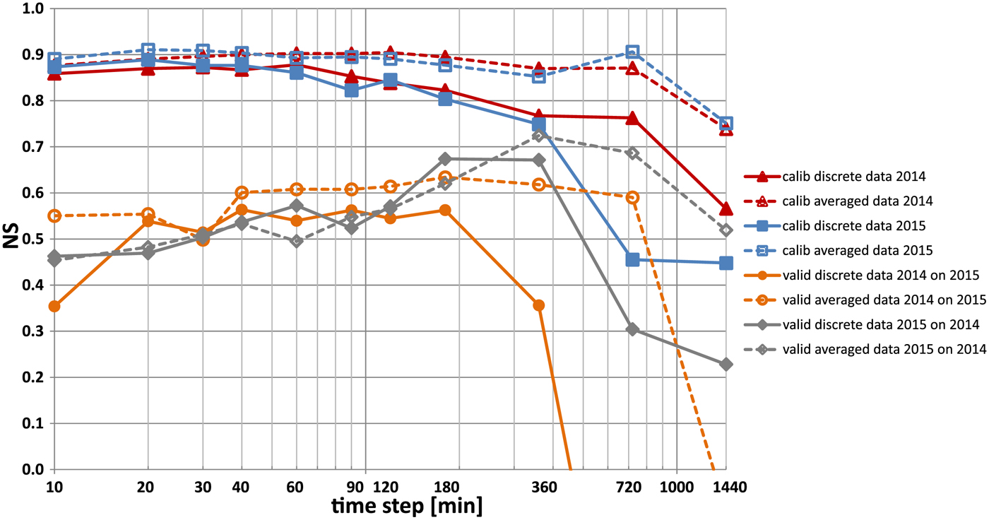
The best calibration and validation results from 30 runs of optimization procedure using HBV model for discrete and time-averaged hydro-meteorological data are presented in Figure 5. It is visible that in almost all cases, a better fit was obtained for averaged data (shown as dotted lines) than for discrete data (shown as continuous lines). Differences in the model fit are larger for longer time intervals (360, 720 and 1440 min). The results of model validation for both seasons, higher than 0.50, were obtained for averaged over time intervals between 30 and 720 min. The best fit at validation stage (NS = 0.72) was estimated for 360 min for model from year 2015 validated on data from year 2014.
Comparison of the best calibration and validation results from 30 runs of optimization procedure for discrete (continuous lines) and averaged (dotted lines) over time step data.
The influence of input data averaging on the spread of NS values obtained at 30 runs of calibration procedure was also tested. The results in the form of boxplots are shown in Figure 6. A comparison of the outcomes for averaged (Fig. 6) and discrete input data (Fig. 4) indicate that application of averaged data resulted in a higher median from 30 runs of the optimization procedure for almost all time steps and seasons. The highest improvements in median NS were obtained for 1, 6, 12 and 24 h time step.
A comparison of the calibration (upper row of panels) and validation results (bottom row of panels) for averaged data from year 2014 (panels on the left) and 2015 (panels on the right). Boxplots present the NS obtained for different data time step. In each boxplot, the bottom and top of the box represent the first and third quartiles and the red line inside the box represents the median. The error bars represent the minimum and maximum from 30 runs of calibration procedure.

The effect of time step on parameter values
The obtained results of multiple runs of model calibration allowed for analysis of data time step on the model parameters. Those analyses were carried out independently for two seasons (2014 and 2015) and for discrete and averaged input data. Scatterplots showing the influence of data time step on 13 HBV model parameters are presented in Figure 7. The optimum values of KF, KS, PERC, CFLUX and CFMAX were transformed into the same units (1 day−1, 1 day−1, mm day−1, mm day−1 and mm °C day−1, respectively).
Dependence of discrete (blue lines) and averaged (red lines) parameter values on time step of data.

It is shown that the relationships depend on parameter and also on the season and data averaging. These results allowed for classification of the parameters into a few groups. In the first group of parameters (KF, PERC, ALFA and CFMAX), consistent changes of parameter values together with an increase of time step is visible for both seasons and for discrete or averaged input data. Little change of the input data with time was found for KS, TT, FC and BETA. The third group of parameters (CFR, TTI, WHC, and CFLUX) had no consistent dependences between time step and parameter values.
In addition to visual inspection, the results were quantified using a variance decomposition technique following an analysis of variance (ANOVA) approach (Von Storch and Zwiers, Reference Von Storch and Zwiers2001). We considered the following ANOVA model:
 $$\eqalign{{\rm IN}_{ijk} &= \mu + {\rm TS}_i + {\rm YR}_j + {\rm FI}_k + ({\rm TS} \times {\rm YR})_{ij} \cr&\quad + ({\rm TS} \times {\rm FI})_{ik} + ({\rm YR} \times {\rm FI})_{\,jk} + \varepsilon _{ijk}} $$
where IN ijk is a value of parameter (e.g. FC) for ith time step (10, 20 min, …, 24 h), jth year (2014, 2015) and kth data averaging (without/with). The first element on the right-hand side of Eqn (2) denotes the overall mean. The next three elements represent the principal contributions to the variance corresponding to the time step (TS), year (YR) and data averaging (FI). The following three elements describe the interactions between them (TS × YR, TS × FI, YR × FI). The last element represents errors (i.e. the unexplained variance). The N-way ANOVA analysis was supplemented by Tukey's honestly significant difference criterion procedure (Tukey, Reference Tukey1949) to test the equality of the mean response for groups. The results of the test allowed for statistical comparison of differences between time steps, seasons and data averaging.
According to N-way ANOVA and Tukey test, statistically significant differences between two analyzed seasons (years 2014 and 2015) were found for all parameters but CFMAX. The opposite results of testing were obtained for the case of data averaging. There are no differences in parameter values for the averaged and discrete data for all parameters but CFR. Differences in parameter values between time steps were estimated as statistically significant for BETA, ALFA, KF, KS, PERC and TT. For other parameters (FC, LP, CFLUX, TTI, CFMAX, CFR, WHC), there are no statistically significant differences in optimum values between different time steps.
SUMMARY AND CONCLUSION
This paper presents results of catchment run-off modelling in the Arctic unglaciated catchment using the HBV model. The estimated value of the TC by the Kirpich formula was ~10 min. Therefore, it was assumed as an initial choice of time step for catchment run-off modelling. As the estimates of TC are highly biased, the analysis included an aggregation of hydro-meteorological input data to 20, 30, 40, 60 and 90 min; 2, 3, 6, 12 and 24 h.
High-quality 10 min time step discharge measurements, precipitation and air temperature data were available for Fuglebekken catchment for two ablation seasons (2014 and 2015), which made testing an influence of data time step on the calibration and validation results as well as values of parameters possible. HBV has 13 parameters calibrated on discharge measurements from 2014 and 2015 separately and verified on both years independently.
The obtained results (best fit from 30 runs of optimization procedure by DEGL method) indicated that calibration and validation results depend on the time step and season. Better results of calibration were obtained for year 2015. In the case of validation, higher NS values were obtained for model from year 2015 validated on data from year 2014. These differences in model performances could be explained by the hydro-meteorological conditions in the catchment in these two seasons. The ablation season 2014 and in particular August 2014 was very dry, almost without precipitation events throughout the month. As a result, for a few days, after 20 August, water ceased to flow in the channel. Such conditions led to the weaker identifiability of the model parameters and worse calibration and validation results.
A comparison of the calibration and validation results between different time steps indicated that the best results for the model from year 2015 were obtained for 3 and 6 h. Those time steps are recommended for further use in hydrological simulations, though the time steps differ significantly from the estimated TC value (10 min). These differences could be explained by the higher observation errors at smaller time steps than for aggregated data. Aggregation and data averaging lead to improvement of model performance. Such behaviour is visible for time steps up to 6 h. Further increases in time step cause a decrease in NS values.
The chosen calibration procedure (30 runs of the DEGL method) allowed for analysis of spread in the objective function (NS values). These results indicate that there is a significant spread in the NS values that depends on the time step and season. The outcomes indicate that for catchment modelling for the Fuglebekken catchment, the DEGL algorithm converged to the local optima. This problem occurred more frequently for smaller time steps. Therefore, multiple runs of optimization procedure are required for finding global optimum.
The results of analyzing the influence of input data averaging, input data temporal resolution, and calibration season (2014 and 2015) on the modelling results were tested using N-way ANOVA analysis supplemented with Tukey test. The outcomes of such testing indicated that input data averaging has a statistically significant influence on the obtained values of objective function (NS values) but not on the values of the HBV model parameters. The population marginal means of model parameters are not statistically different for instantaneous and averaged input data.
Statistically significant differences between two analyzed seasons (years 2014 and 2015) were found for all parameters but CFMAX. No differences in parameter values were found for data with and without averaging for all parameters except CFR. In case of time steps, statistically significant differences between parameter values were estimated for BETA, ALFA, KF, KS, PERC and TT.
The obtained results may partially depend on the objective function used during model calibration, validation and optimization method. In this study, the Nash-Sutcliffe objective function was applied. That choice results in better fit of high and mean discharges and poor performance in low discharges. In addition, the presented results may be influenced by overparametrization of the model, which could lead to poor parameter identification and increased uncertainty. In this study, we applied full version of the model; however, the results of sensitivity analysis by the Sobol method indicated that mainly three parameters (KS, BETA and FC) have significant influence on model fit (Nash-Sutcliffe values). The influence of other parameters is small. We have found that the estimated values of sensitivity indices depend on the time step. The choice of full model instead of simplified one was dictated by the differences of obtained sensitivity indexes between years (2014 and 2015) and differences in input data (instantaneous and averaged). It is important to mention than the sensitivity analysis as well as model calibration and validation were performed for model output aggregated over the full time series of discharges. We suspect that an influence of parameters is also varying with time as it is presented by Pianosi and Wagener (Reference Pianosi and Wagener2016).
Hydrological modelling presented in this paper leads to the development of knowledge about the temporal and spatial variability of water balance components in non-glaciated Arctic catchments. Significant results of calibration and validation were obtained, which can justify the application of the HBV model in other years at Fuglebekken catchment and may give the opportunity to assess the actual state, as well as simulate future changes in other areas of the circumpolar zone.
ACKNOWLEDGEMENTS
The financial support for this work has been provided by the Polish National Science Centre through grant No. 2013/09/N/ST10/04105. This work was also partially supported by the Institute of Geophysics, Polish Academy of Sciences within statutory activities No 3841/E-41/S/2017 of the Ministry of Science and Higher Education of Poland and from the funds of the Leading National Research Centre (KNOW) received by the Centre for Polar Studies for the period 2014–18. The meteorological data were provided by the Hornsund Polish Polar Station and the Institute of Geophysics, Polish Academy of Sciences. We are grateful to two anonymous reviewers for valuable comments on the manuscript. We are also very grateful to Melissa Wrzesien for improving the English.


 Open access