


1. Introduction
Taylor (Reference Taylor1964) described the hydrostatic structure of the so-called Taylor cone through the balance between capillary and electrostatic stresses on the surface of an equipotential cone. The cone angle  $\alpha _T=49.29^{\circ }$ is fixed after demanding that the surface be equipotential. Although this solution is much simpler than the hydrodynamic cone-jet mode of electrospray (Gañán-Calvo et al. Reference Gañán-Calvo, López-Herrera, Herrada, Ramos and Montanero2018), it exhibits many features of that mode, provides information about the far-field affecting the jet dynamics in electrospray (Gañán-Calvo Reference Gañán-Calvo1997), and allows insight to be gained into some observed phenomena of this atomization technique.
In general, the hydrostatic solution derived by Taylor (Reference Taylor1964) cannot be adopted when ejection takes place. When this ejection occurs in the form of a steady jet and the resulting charged aerosol (Fenn Reference Fenn1993), the mass and (most fundamentally) charge withdrawal elicits an internal electric field, and, consequently, shear electric stresses on the interface. These stresses provoke steady, sometimes vigorous internal motions by viscous diffusion of momentum (Barrero et al. Reference Barrero, Gañán-Calvo, Dávila, Palacios and Gómez-González1999). Thus, the inescapable charge circulation associated with a Taylor cone-jet makes the hydrostatic solution non-physical. In addition, when the cone consists of two immiscible liquids with finite conductivities, the Taylor solution is even more unrealistic because the two interfaces cannot form the same cone with the angle  $\alpha _T$. In this case, an electric field necessarily arises inside the shapes adopted by the interfaces, even in the absence of ejections. Ramos & Castellanos (Reference Ramos and Castellanos1994) calculated the self-similar Stokes flow caused by an external electric field in a Taylor cone of a leaky-dielectric liquid in a leaky-dielectric bath.
The understanding of the electrohydrodynamic phenomena taking place in double or coaxial Taylor cones (Loscertales et al. Reference Loscertales, Barrero, Guerrero, Cortijo, Marquez and Gañán-Calvo2002) is of great importance at both fundamental and technological levels. This microfluidic structure opened a door to explore new and creative materials (microcapsules, microfibres, emulsions, etc.) in a wide variety of fields from pharmacy to the chemical or textile industry (Lauricella et al. Reference Lauricella, Succi, Zussman, Pisignano and Yarin2020). For instance, the development of highly dielectric elastomers for their application as dielectric actuators in novel electromechanical, biomedical and biomechanical devices constitutes an important application, which is critically dependent on the internal microstructure of the materials (Mazurek et al. Reference Mazurek, Yu, Gerhard, Wirges and Skov2016). The only possibility for strict control on the formation of double emulsions beyond the well-known dripping-jetting limit imposed by charge relaxation phenomena (Gañán-Calvo et al. Reference Gañán-Calvo, López-Herrera, Herrada, Ramos and Montanero2018) is to have stable double Taylor cones that could survive as such, in the absence of emission, with the maximum possible curvature at the apex. This entails the existence of electrohydrodynamic coaxial-cone solutions incorporating the full spectrum of phenomena associated with the flow of liquids and charges, which is not allowed by the original, single-cone Taylor solution.
The Taylor–Melcher leaky-dielectric model (Melcher & Taylor Reference Melcher and Taylor1969) has proved to be a useful tool to study the dynamical behaviour of poorly conducting droplets in poorly conducting or dielectric baths. In particular, it provides accurate predictions for the steady cone-jet mode of electrospray (Gañán-Calvo Reference Gañán-Calvo1997; Fernández de la Mora Reference Fernández de la Mora2007; Higuera Reference Higuera2010; Ponce-Torres et al. Reference Ponce-Torres, Rebollo-Muñoz, Herrada, Gañán-Calvo and Montanero2018), and can be used to simulate ionic-liquid menisci undergoing evaporation of ions (Higuera Reference Higuera2008). This model assumes that all the net free charge accumulates at the interface within a Debye layer much thinner than the system size. It also considers the ohmic model to account for the conduction through the liquid bulk and across the Debye layer. In this paper, we will solve analytically the leaky-dielectric model to calculate the self-similar Stokes flow driven by the electric field in a multiple Taylor cone comprising immiscible low-conductivity or dielectric fluids. First, we will obtain a solution valid for sufficiently large distances from the cone vertex so that charge convection over the interface can be neglected vs conduction across it. Then, we will include surface charge convection in coaxial Taylor cones to extend the validity of the self-similar solution to the vicinity of the cone vertex. We will illustrate the relevance of the present analytical approach by considering some examples with potential technological applications, such as the production of encapsulated microbubbles by electrohydrodynamic means.
2. Governing equations and self-similar solution
2.1. Governing equations
Consider the multiple Taylor cone sketched in figure 1. The shadowed labels  $j=0,1,\ldots ,J$ denote the $J+1$ phases involved in the problem, while the non-shadowed labels $j=1,2,\ldots ,J$ denote the interfaces between the phases $j-1$ and $j$. The phases are leaky-dielectric or dielectric viscous fluids with electrical permittivities $\varepsilon ^{(0)}, \varepsilon ^{(1)}, \ldots , \varepsilon ^{(J)}$, electrical conductivities $K^{(0)}, K^{(1)}, \ldots , K^{(J)}$ and dynamical viscosities $\mu ^{(0)}, \mu ^{(1)}, \ldots , \mu ^{(J)}$, respectively. The interfaces are characterized by the surface tensions $\gamma _1, \gamma _2, \ldots , \gamma _J$. We make use of the spherical coordinate system with the symmetry axis $\theta =0$, as indicated in figure 1. The locations of the interfaces are characterized by the angles $\theta =\alpha _1, \alpha _2, \ldots , \alpha _J$. In what follows, the superscript $j=0,1,\ldots ,J$ indicates the domain where the corresponding quantity is evaluated, while the subscript $j=1,2,\ldots ,J-1$ indicates the interface.
Sketch of the fluid configuration.

We select the length, time, mass and electric charge units so that  $\mu ^{(1)}=\gamma _1=\kappa ^{(1)}=\varepsilon ^{(1)}=1$. Consequently, the problem can be formulated in terms of the permittivities, conductivities and viscosity ratios $\beta ^{(j)}=\varepsilon ^{(j)}/\varepsilon ^{(1)}$, $\kappa ^{(j)}=K^{(j)}/K^{(1)}$ and $\lambda ^{(j)}=\mu ^{(j)}/\mu ^{(1)}$ ( $j\neq 1$), as well as the surface tension ratios $\varGamma _j=\gamma _j/\gamma _1$ ( $j\neq 1$). With the above choice, the electric relaxation time $t_e=\varepsilon ^{(1)}/K^{(1)}$ in the phase $j=1$ equals unity.
The stream function characterizing the Stokes flow in each fluid domain,  $\varPsi ^{(j)}(r,\theta )$, obeys the linear partial differential equation
 \begin{equation} E^2(E^2 \varPsi^{(j)})=0, \end{equation}
where the differential operator  $E^2$ is given by the expression
 \begin{equation} E^2\equiv \frac{\partial^2}{\partial r^2}+\frac{\sin\theta}{r^2}\frac{\partial}{\partial \theta}\left(\frac{1}{\sin\theta}\frac{\partial}{\partial\theta}\right). \end{equation}
The radial and angular components of the velocity field are calculated from the stream function as
 \begin{equation} v_r^{(j)}=\frac{1}{r^2\sin\theta}\frac{\partial\varPsi^{(j)}}{\partial\theta},\quad v_\theta^{(j)}={-}\frac{1}{r\sin\theta}\frac{\partial\varPsi^{(j)}}{\partial r}. \end{equation}
In the leaky-dielectric approximation, the net free charge in the bulk is assumed to be zero, and, therefore, the Laplace equation
 \begin{equation} \nabla^2 \phi^{(j)}=0 \end{equation}
for the electric potential  $\phi ^{(j)}(r,\theta )$ applies to all the phases. The radial and angular components of the electric field are calculated as
 \begin{equation} E_r^{(j)}={-}\frac{\partial\phi^{(j)}}{\partial r}, \quad E_\theta^{(j)}={-}\frac{1}{r}\frac{\partial\phi^{(j)}}{\partial \theta}. \end{equation}
The interfaces are streamlines, and the radial component of the velocity field takes the same value on the two sides of them. Therefore,
 \begin{equation} v_\theta^{(j-1)}(r,\alpha_{j})=v_\theta^{(j)}(r,\alpha_{j})=0, \quad v_r^{(j-1)}(r,\alpha_{j})=v_r^{(j)}(r,\alpha_{j}), \quad j=1,2,\ldots, J. \end{equation}
The difference between the normal stresses on the two sides of the interface is balanced by the corresponding capillary pressure, which yields
 \begin{align} &-p^{(j-1)}(r,\alpha_{j})+\tau_{\theta\theta}^{(j-1)}(r,\alpha_{j})+\tau_{M\theta\theta}^{(j-1)}(r,\alpha_{j})-\varGamma_{j}\hat{\kappa}_{j}\nonumber\\ &\quad ={-}p^{(j)}(r,\alpha_{j})+\tau_{\theta\theta}^{(j)}(r,\alpha_{j})+\tau_{M\theta\theta}^{(j)}(r,\alpha_{j}), \quad j=1,2,\ldots, J, \end{align}
where  $p^{(j)}(r,\theta )$ is the hydrostatic pressure,
 \begin{equation} \tau_{\theta\theta}^{(j)}=\frac{2\lambda^{(j)}}{r}\left(\frac{\partial v_\theta^{(j)}}{\partial\theta}+v_r^{(j)}\right)\quad \text{and} \quad \tau_{M\theta\theta}^{(j)}=\frac{\beta^{(j)}}{2}\left[\left(E_\theta^{(j)}\right)^2-\left(E_r^{(j)}\right)^2\right] \end{equation}
are the viscous and Maxwell normal stresses, respectively, and  $\hat {\kappa }_j=1/(r\tan \alpha _j)$ is the local mean curvature of the $j$th interface. The continuity of the tangential stresses at the interfaces leads to
 \begin{equation} \tau_{r\theta}^{(j-1)}(r,\alpha_{j})+\tau_{Mr\theta}^{(j-1)}(r,\alpha_{j})=\tau_{r\theta}^{(j)}(r,\alpha_{j})+\tau_{Mr\theta}^{(j)}(r,\alpha_{j}), \quad j=1,2,\ldots, J, \end{equation}
where
 \begin{equation} \tau_{r\theta}^{(j)}=\lambda^{(j)}\left[r\frac{\partial}{\partial r} \left(\frac{v_\theta^{(j)}}{r}\right)+\frac{1}{r}\frac{\partial v_r^{(j)}}{\partial\theta}\right] \quad \text{and} \quad \tau_{Mr\theta}^{(j)}=\beta^{(j)} E_r^{(j)} E_\theta^{(j)} \end{equation}
are the viscous and Maxwell tangential stresses, respectively.
The continuity of the tangential component of the electric field at the interface leads to
 \begin{equation} E_r^{(j-1)}(r,\alpha_{j})=E_r^{(j)}(r,\alpha_{j}), \quad j=1,2,\ldots,J. \end{equation}
In addition, the difference between the normal components of the electric field displacement on the two sides of the interface equals the surface charge density:
 \begin{equation} \beta^{(j-1)} E_\theta^{(j-1)}(r,\alpha_{j})-\beta^{(j)} E_\theta^{(j)}(r,\alpha_{j})=\sigma_{j}(r), \quad j=1,2,\ldots, J, \end{equation}
where  $\sigma _j(r)$ is the surface charge density at the $j$th interface. The surface charge conservation at the interface leads to
 \begin{align} &2{\rm \pi} r\sin\alpha_{j} \left[\kappa^{(j-1)} E_\theta^{(j-1)}(r,\alpha_{j})-\kappa^{(j)} E_\theta^{(j)}(r,\alpha_{j})\right]\nonumber\\ &\quad =\frac{\textrm{d}}{\textrm{d}r}\left[2{\rm \pi} r\sin\alpha_{j} \sigma_{j}(r) v_r^{(j)}(r,\alpha_{j})\right], \quad j=1,2,\ldots, J. \end{align}
The right-hand side of (2.13) represents the surface charge convection along the interface. Interestingly, if one assumes that this effect is negligible as compared with charge conduction from/towards the bulk, (2.12) and the surface charge densities are removed from the formulation of the problem, and (2.13) is replaced with (Burcham & Saville Reference Burcham and Saville2002)
 \begin{equation} \kappa^{(j)} E_\theta^{(j)}(r,\alpha_{j})=\kappa^{(j-1)} E_\theta^{(j-1)}(r,\alpha_{j}), \quad j=1,2,\ldots, J. \end{equation}
 In general, as will be seen in § 2.2, the left and right terms of (2.13) scale differently with respect to  $r$. Indeed, while the conduction term dominates for $r\gg 1$, charge convection becomes dominant for $r\ll 1$. Therefore, convection cannot be neglected vs conduction for $r\lesssim 1$. However, for $J>1$ (more than two domains), it is possible to obtain self-similar solutions all the way from $r\sim 1$ to $r\gg 1$ (for $r\ll 1$, the leaky-dielectric fails, as will be explained in § 2.2) in the absence of (or negligible) charge emission from the apex. For this purpose, we apply the Gauss theorem and Laplace equation (2.4) in each domain, which in the absence of emission leads to
 \begin{align} &\int_{0}^{r} 2{\rm \pi} r' \left[\sin\alpha_{j}E_\theta^{(j)}(r',\alpha_{j})- \sin\alpha_{j+1}E_\theta^{(j)}(r',\alpha_{j+1})\right]\textrm{d}r' \nonumber\\ &\quad =\int_{\alpha_{j}}^{\alpha_{j+1}} E_r^{(j)}(r,\theta) 2{\rm \pi} r^2\sin \theta \,\textrm{d}\theta,\quad j=0,1,\ldots,J, \end{align}
where  $\alpha _0={\rm \pi}$ and $\alpha _{J+1}=0$ (note that the numbering of $\alpha _j$ is opposite to the increment of $\theta$). In addition, the integration of (2.13) from 0 to $r$ yields
 \begin{align} &\int_0^r 2{\rm \pi} r' \sin\alpha_{j}\left[\kappa^{(j-1)} E_\theta^{(j-1)}(r',\alpha_{j})-\kappa^{(j)} E_\theta^{(j)}(r',\alpha_{j})\right]\textrm{d}r'\nonumber\\ &\quad =2{\rm \pi} r\sin\alpha_{j}\sigma_{j}(r) v_r^{(j)}(r,\alpha_{j}), \quad j=1,2,\ldots,J, \end{align}
where we have taken into account that  $r\sigma v_r=0$ for $r=0$, as will be seen in § 2.2. If we multiply (2.15) by $\kappa ^{(j)}$ and sum up (2.15) and (2.16) for all the domains, we obtain
 \begin{equation} \sum_{j=0}^{J} \left[\kappa^{(j)} \int_{\alpha_{j}}^{\alpha_{j+1}} E_r^{(j)}(r,\theta) 2{\rm \pi} r^2\sin (\theta) \,\textrm{d}\theta + 2{\rm \pi} r \sin\alpha_{j}\sigma_{j}(r) v_r^{(j)}(r,\alpha_{j})\right]=0, \end{equation}
where  $\sigma _{0}=\sigma _{J+1}=0$. This equation expresses that the sum of bulk conduction (left term) and surface convection (right term) across the sphere surface of radius $r$ must be zero in the steady regime. As will be shown in § 2.2, the conduction and convection terms in (2.17) scale as $r^{3/2}$ and $r^{1/2}$ for the self-similar solution, respectively. Therefore, those two terms must be zero independently, i.e.
 \begin{equation} \sum_{j=0}^{J} \kappa^{(j)} \int_{\alpha_{j}}^{\alpha_{j+1}} E_r^{(j)}(r,\theta) 2{\rm \pi} r^2\sin (\theta) \,\textrm{d}\theta=0, \quad \sum_{j=0}^{J} 2{\rm \pi} r \sin\alpha_{j}\sigma_{j}(r) v_r^{(j)}(r,\alpha_{j})=0. \end{equation}
Equation (2.18b) establishes that the sum of the charge convected by all the interfaces at a distance  $r$ from the vertex is zero. In the absence of charge emission, if $J=1$, the charge convected along the only interface is, therefore, zero, and (2.14) verifies.
2.2. Self-similar solution
Equations (2.1) admit solutions of the separable form  $\varPsi ^{(j)}(r,\theta )=r^{m+2} F_m^{(j)}(\theta )$, where $F_m^{(j)}(\theta )$ is the solution to
 \begin{equation} \left[(m+2)(m+1)+(1-x^2)\frac{\textrm{d}^2}{{\textrm{d} x}^2}\right]\times\left[m(m-1)+(1-x^2)\frac{\textrm{d}^2}{{\textrm{d} x}^2}\right]F_m^{(j)}(x)=0, \end{equation}
and  $x=\cos \theta$. Due to (2.7), we necessarily search for the self-similar solution $m=0$, i.e. that leading to a velocity field independent from the radial coordinate $r$. In this case, we obtain
 \begin{align} F_0^{(j)}(x)&=a_1^{(j)} (1-x^2)^{1/2} P_1^1(x)+a_2^{(j)} (1-x^2)^{1/2} Q_1^1(x)+a_3^{(j)}+a_4^{(j)} x\nonumber\\ &=c_1^{(j)}+c_2^{(j)} x+c_3^{(j)} x^2+c_4^{(j)}(1-x^2)\, \text{atanh}(x), \end{align}
where  $P_1^1(x)$ and $Q_1^1(x)$ are the associated Legendre functions, and $a_k^{(j)}$ and $c_k^{(j)}$ ( $k=1$, 2, 3 and 4) are arbitrary constants. The regularity condition for $v_{r}^{(0)}({\rm \pi} )$ and $v_{r}^{(J)}(0)$ yields
 \begin{equation} c_4^{(0)}=0, \quad c_4^{(J)}=0, \end{equation}
respectively. The regularity condition for  $v_{\theta }^{(0)}({\rm \pi} )$ and $v_{\theta }^{(J)}(0)$ yields
 \begin{equation} c_1^{(0)}-c_2^{(0)}+c_3^{(0)}=0, \quad c_1^{(J)}+c_2^{(J)}+c_3^{(J)}=0. \end{equation}
The velocity field (2.3a,b) calculated from the above solution verifies the momentum equation
 \begin{equation} -\boldsymbol{\nabla} p^{(j)}+\lambda^{(j)}\nabla^2 {\boldsymbol{v}}^{(j)}=0, \end{equation}
which yields the pressure field
 \begin{equation} p^{(j)}(r)=p_\infty+\frac{2\lambda^{(j)}(c_2^{(j)}-c_4^{(j)})}{r}, \end{equation}
where  $p_\infty$ is the pressure for $r\to \infty$. This pressure takes the same value for all the phases because (2.7) is satisfied with $\kappa _i,\tau _{\theta \theta }^{(j)}, \tau _{M\theta \theta }^{(j)}\to 0$ as $r\to \infty$.
The Laplace equation (2.4) admits solutions of the separable form
 \begin{equation} \phi^{(j)}(r,\theta)=r^{m+1/2} \varPhi_m^{(j)}(\theta), \end{equation}
where  $\varPhi _m^{(j)}(\theta )$ is the solution to
 \begin{equation} (1-x^2)\frac{\textrm{d}^2\varPhi_m^{(j)}}{{\textrm{d} x}^2}-2x\frac{\textrm{d}\varPhi_m^{(j)}}{\textrm{d} x}+\left(m+\frac{1}{2}\right)\left(m+\frac{3}{2}\right)\varPhi_m^{(j)}=0. \end{equation}
Again, we select the solution for  $m=0$ because in this case $E_r^{(j)},E_\theta ^{(j)}\propto r^{-1/2}$, and then the radial dependence of the Maxwell stresses, $\tau _{M\theta \theta }^{(j)},\tau _{Mr\theta }^{(j)}\propto r^{-1}$, is the same as that of the viscous and capillary ones. The solution of (2.26) for $m=0$ is
 \begin{equation} \varPhi_0^{(j)}=A_1^{(j)} P_{1/2}(x)+A_2^{(j)} Q_{1/2}(x), \end{equation}
where  $P_{1/2}(x)$ and $Q_{1/2}(x)$ are the associated Legendre polynomials, and $A_1^{(j)}$ and $A_2^{(j)}$ ( $j=1,2,\ldots ,J$) are arbitrary constants. The regularity condition for this solution leads to
 \begin{equation} A_1^{(0)}=A_2^{(J)}=0. \end{equation}
 As anticipated, if surface charge convection is neglected (2.14), the radial dependence of all the quantities involved in the boundary conditions cancels out. Therefore, the boundary and regularity conditions constitute a system of  $7\times J+6$ algebraic linear equations for the $6\times (J+1)$ unknowns
 \begin{equation} \{c^{(j)}_k;A_{\ell}^{(j)}\} \quad j=0,1,\ldots J, \quad k=1,2,3\text{ and } 4, \quad \ell=1\text{ and } 2. \end{equation}
The angles  $\alpha _j$ ( $j=1,2,\ldots ,J)$ are the eigenvalues for which that system of equations admits a non-trivial solution. This solution is a function of the properties of the fluids exclusively. It should be noted that neglecting surface charge convection in (2.14) allows one to decouple the hydrodynamic and electric problems for given values of the cone angles. Then, the Laplace equation for the electric potential together with the boundary and regularity conditions for the electric field constitute a closed homogeneous system of linear equations. The determinant $\varDelta (\kappa ^{(0)},\kappa ^{(2)},\ldots ,\kappa ^{(J)};\alpha _1,\alpha _2,\ldots ,\alpha _J)$ (note that $\kappa ^{(1)}=1$) of the matrix associated with that system must be zero to obtain a non-trivial solution of the problem, from which one may obtain a relationship as $\alpha _1=f(\alpha _2,\alpha _3,\ldots ,\alpha _J;\kappa ^{(0)},\kappa ^{(2)},\ldots ,\kappa ^{(J)})$. If $J=1$ (two domains), the condition $\varDelta =0$ leads to $\alpha _1=f(\kappa ^{(0)})$ or $\kappa ^{(0)}=\kappa ^{(0)}(\alpha _1)$. This function will be plotted in § 3.
If one adopts the self-similar solution derived above, the conduction and convection terms in (2.13) scale as  $r^{1/2}$ and $r^{-1/2}$, respectively (or as $r^{3/2}$ and $r^{1/2}$ in (2.17)). Therefore, surface convection cannot be neglected vs conduction for $r\lesssim 1$, and the self-similar solution ceases to be valid in that region. However, the intermediate region $r\sim 1$ is scientifically and technologically relevant since the existence of solutions valid for this region would open ways to extend significantly the range of operation of current electrospray systems for very small flow rates or size of ejecta, or to develop novel systems with highly non-linear voltage-current responses, among many other possible new ideas. To extend the validity of the solution down to $r\sim 1$ (for $r\ll 1$ the leaky-dielectric fails, as explained below), we replace (2.14) with the integral equation (2.17) for the total charge both conducted and convected across the sphere of radius $r$. In this integral equation, the conduction and convection terms scale as $r^{3/2}$ and $r^{1/2}$, respectively. Therefore, those two terms must be zero independently to obtain a self-similar solution. Thus, for $J=2$, one may alternatively consider the two integral equations (2.18a,b) instead of the two interface equations of the form (2.14). Despite its realization being yet unclear, the solution of this problem opens up a beautiful possibility: that instead of a charge ejection issuing from the cone vertex, the system may internally drain the charges through the innermost liquid domain. In fact, the existence of an inner liquid drain (i.e. the inner J-domain) is the only way to have a non-emitting self-similar (conical) electrohydrodynamic solution in an outer dielectric medium, a possibility excluded in the original Taylor solution. In other words, in a steady regime and from a global charge balance perspective, the role of the inner drain would be equivalent to that of an emitted jet, but in the opposite direction. To have this, the intermediate medium $j=1$ should resist electric breakdown, a condition met by many low-conductivity (leaky-dielectric) liquids for the maximum electric fields here considered, which are of the order of $E_o=(\mu ^{(1)}K^{(1)})^{1/2}/\varepsilon ^{(1)}$ (e.g. $1\ \textrm {MV}\ \textrm {m}^{-1}$ for distilled water, well below its electric breakdown of ${\sim }70\ \textrm {MV}\ \textrm {m}^{-1}$).
In any case, the solution derived above fails for sufficiently small distances from the cone vertex ( $r\ll 1$) for two reasons. First, the condition $\delta /r\ll 1$ ( $\delta$ is the Debye length) is a geometrical requisite to justify the interfacial nature of the leaky-dielectric model (Russel, Saville & Schowalter Reference Russel, Saville and Schowalter1991; Gañán-Calvo et al. Reference Gañán-Calvo, López-Herrera, Herrada, Ramos and Montanero2018). Second, the electric field diverges as the distance to the vertex goes to zero. Then, the equilibrium in the Debye layer is perturbed by the applied electric field for sufficiently small values of $r$, which prevents the ohmic conduction through that layer (Russel et al. Reference Russel, Saville and Schowalter1991).
3. Discussion and results
In this section, we present some illustrative results obtained (i) by neglecting charge convection over the interface vs ohmic conduction across it (2.14) (solution of Type I), and (ii) by setting both the charge conducted and convected across a sphere of radius  $r$ equal to zero (2.18a,b) (solution of Type II). As explained in § 2.2, the equations leading to the solution of Type II reduce to those of Type I, and therefore charge convection over the interface is necessarily neglected.
When  $J=1$, there is a unique relationship $\kappa ^{(0)}(\alpha _1)$ for the self-similar solution of Type I (valid for $r\gg 1$) to exist (figure 2a). As can be seen, non-emitting self-similar solutions exist only for $0<\alpha _1<\alpha _T=0.860274\ldots$ Interestingly, there is a maximum value of the conductivity ratio $\kappa _{{max}}^{(0)}=0.0568226\ldots$ , which corresponds to $\alpha _1^*=0.523599\ldots$ . For conductivity ratios in the interval $0<\kappa ^{(0)}<\kappa _{{max}}^{(0)}$, there are two possible solutions: one for a lower voltage decay and another for a higher one. These solutions correspond to a larger and smaller value of $\alpha _1$, respectively, depending on the ratio of permittivities $\beta ^{(0)}$. Figure 2(b) shows an example for $\alpha _1>\alpha _1^*$. These results coincide with those obtained by Ramos & Castellanos (Reference Ramos and Castellanos1994), which constitutes a validation of our calculations.
Solution for  $J=1$. (a) The function $\kappa ^{(0)}(\alpha _1)$, and (b) solution for $\beta ^{(1)}=3.5$, $\lambda ^{(0)}=0.1$ and $\alpha _1=0.7$, which corresponds to $\kappa ^{(0)}=0.0426335\ldots$ . The continuous lines are the streamlines, while the dashed lines are the equipotential lines. The electric potential is re-scaled so that the maximum value in the figure is 1. The white line is the interface.

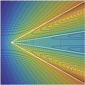
For  $J=2$, the electrohydrodynamic solution depends on seven parameters: $\{\varGamma _2, \beta ^{(0)}, \beta ^{(2)}, \kappa ^{(0)}, \kappa ^{(2)}, \lambda ^{(0)}, \lambda ^{(2)}\}$. Given the immense variety of possible solutions, we have selected a few examples to illustrate cases of technological relevance and novelty. Figure 3(a) shows the resulting angles $\alpha _1$ and $\alpha _2$ for solutions of Type I given values of the conductivities: isocontours $\kappa ^{(0)}=$const. are plotted for fixed values of $\kappa ^{(2)}$ as a function of $\alpha _1$ and $\alpha _2$. As explained in § 2.2, the results are calculated from the solvability condition $\varDelta (\kappa ^{(0)},\kappa ^{(2)};\alpha _1,\alpha _2)=0$ for the electric problem.
(a) Isocontours of  $\kappa ^{(0)}=\textrm {const}$. calculated from solutions of Type I for $J=2$ and fixed values of $\kappa ^{(2)}$ as a function of $\alpha _1$ and $\alpha _2$. (b) Isocontours of $\kappa ^{(3)}=\textrm {const}$. calculated from solutions of Type I for $J=3$ and fixed values of $\kappa ^{(0)}$, $\kappa ^{(2)}$ and $\alpha _3$ as a function of $\alpha _1$ and $\alpha _2$.

Among the non-emitting, self-similar double Taylor cones with technological relevance, the case of an inner ( $j=2$) gas domain with $\beta ^{(0)}<1$, $\kappa ^{(2)}=0$ and $\lambda ^{(2)}\ll 1$ is of particular importance since the electrohydrodynamic generation of micrometre bubbles from steady Taylor cones has not been possible so far, and the solutions here proposed may open a way to produce them. Figure 4 shows two examples of solutions of Type I including the case of a gaseous core. It is worth mentioning that self-similar solutions of Type I cannot be found for all possible configurations. It can be seen that for $J=2$ (three domains), the outer phase $j=0$ cannot be a dielectric medium ( $\kappa ^{(0)}\neq 0$) for the non-trivial solution to exist. This means that the two fluids occupying the region $\theta <\alpha _1$ should be connected to relatively close voltages. In this configuration, the phases and interfaces $j=1$ and 2 drive charges in the same direction, while the outer medium drains charges in the opposite one. In the absence of liquid ejection (e.g. a charged aerosol), ohmic conduction through the bulk is the only transport mechanism from the source to the drain.
Solutions for  $J=2$. (a) Type I, two viscous liquids in a low viscosity, low permittivity, outer liquid: $\varGamma _2=0.2$, $\beta ^{(0)}=0.05$, $\beta ^{(2)}=1$, $\lambda ^{(0)}=0.5$, $\lambda ^{(2)}=0.002$, $\kappa ^{(0)}=0.02$ and $\kappa ^{(2)}=0.02$, which yields $\alpha _1=0.5567$ and $\alpha _2=0.4462$. (b) Type I, with an inner ( $j=2$) gas domain: $\varGamma _2=2$, $\beta ^{(0)}=0.0217$, $\beta ^{(2)}=0.011$, $\lambda ^{(0)}=0.2$, $\lambda ^{(2)}=0.001$, $\kappa ^{(0)}=0.05357$ and $\kappa ^{(2)}=0$, which yields $\alpha _1=0.471503$ and $\alpha _2=0.08982$. (c) Type II, with an outer ( $j=0$) gas domain: $\varGamma _2=1$, $\beta ^{(0)}=0.3135$, $\beta ^{(2)}=2.26$, $\lambda ^{(0)}=0.007$, $\lambda ^{(2)}=1$, $\kappa ^{(0)}=0$ and $\kappa ^{(2)}=10$, which yields $\alpha _1=0.51043$ and $\alpha _2=0.1497$. The continuous lines are the streamlines, while the dashed lines are the equipotential lines. The electric potential is re-scaled so that the maximum value in the figure is 1. The white lines represent the interfaces.

In contrast, when  $J=3$ (four domains), solutions of Type I with an outer dielectric medium (in particular, a gas) can be found, which is not possible for $J=1$ and 2. In other words, configurations with $J\geqslant 3$ are the only ones that allow self-similar solutions of Type I without emission into a gaseous ambient. Figure 3(b) shows examples of resulting cone angles $\alpha _1$ and $\alpha _2$ calculated for different combinations of electrical conductivities and inner cone angle ( $\alpha _3$). One may observe that no solution with $\kappa ^{(0)}=0$ is found when $\kappa ^{(2)}>\kappa ^{(1)}$. On the other hand, the viable values of $\kappa ^{(3)}$ are strongly non-linearly dependent on $\kappa ^{(2)}$.
Solutions of Type II relax the approximation of negligible charge convection over the interfaces, allowing charge convection from one interface to another due to the flow reversal close to the apex ( $r\lesssim 1$) when charge relaxation limit sets in. This mechanism is expected to limit the local electric field. Solutions of Type II allow the existence of double Taylor cones with no charge emission into an outer dielectric (e.g. gas) domain. Figure 4(c) shows an example of these solutions akin to, for example, an intermediate layer of a silicone oil with a core of a glycol of the same viscosity. The electric field in the intermediate domain is even slightly stronger than that in the outer gaseous environment. To have this, the inner and intermediate liquid domains should be connected to voltages with opposite polarities, which (as previously discussed) demands a sufficient dielectric strength from the intermediate liquid. This configuration is particularly relevant since the inner liquid can act as a charge drain if the voltages are selected according to the solution here obtained. If slightly different voltages are applied to the liquids, emissions are expected to take place from the cone tip at scales smaller than unity.
In this work, we have found analytically self-similar electrohydrodynamic solutions without emission in the classical Taylor cone problem. The existence of these solutions is particularly relevant to the technological possibility of emitting tiny droplets close to the conditions of no-emission. In particular, the case  $J=2$ offers two types of voltage setting configurations: solutions Types I and II. A very interesting example of Type I solutions is obtained for two liquids with a gaseous innermost phase. This configuration may allow ejecting microbubbles from that phase into the outer liquid domain with dimensionless sizes below unity. Once dispersed in the outermost medium, these microbubbles would be covered by a layer of liquid drawn from the intermediate domain during the ejection. This would protect them from collapse and coalescence, and would provide them with special mechanical properties. Besides, and under the above-described conditions leading to solutions of Type II with internal charge drain, the system would act as a novel microfluidic triode, which may bring unexpected features for applications ranging from new sensors to mass spectrometry, ultra-high precision deposition or materials syntheses. Both the numerical simulation and experimental realization of these possibilities are beyond the scope of this analytical study, and will be the subject of subsequent works.
Acknowledgements
A.M.G.C. wishes to express his gratitude to his close colleagues M.A. Herrada and J.M. López-Herrera for ongoing and inspiring discussions.
Funding
This research has been supported by the Spanish Ministry of Economy, Industry and Competitiveness (A.M.G.C., J.M.M., grant numbers DPI2016-78887 and PID2019-108278RB); Junta de Andalucía (A.M.G.C., grant number P18-FR-3623); and Junta de Extremadura (J.M.M., grant number GR18175).
Declaration of interests
The authors report no conflict of interest.


 Open access