





1. Introduction
The study of flow dynamics in particle-laden fluids over porous surfaces has attracted substantial attention due to its relevance in a range of natural, biological and industrial systems. In biological contexts, such flows play a critical role in understanding transport mechanisms in blood vessels, the gastrointestinal tract and the renal system (Chang et al. Reference Chang, Ha, Park, Kim and Shin1989; Majdalani, Zhou & Dawson Reference Majdalani, Zhou and Dawson2002; Mirbod, Wu & Ahmadi Reference Mirbod, Wu and Ahmadi2017; Haffner & Mirbod Reference Haffner and Mirbod2020). Similarly, in industrial applications, porous media and particle-laden flows are prevalent in filtration systems, oil recovery processes and chemical reactors, making it essential to comprehensively investigate their stability characteristics (Allen Reference Allen1984; Ewing & Weekes Reference Ewing and Weekes1998; Blest et al. Reference Blest, Duffy, McKee and Zulkifle1999; Perazzo et al. Reference Perazzo, Tomaiuolo, Preziosi and Guido2018). While biological systems motivate the broader relevance of particle-porous interactions, the present formulation is restricted to dilute inertial suspensions and does not attempt to quantitatively model complex suspensions such as blood.
Numerous studies have examined the stability of plane Poiseuille flow in fluid-porous media systems to understand the interaction between fluid dynamics and porous structures. Chang, Chen & Straughan (Reference Chang, Chen and Straughan2006) conducted a linear stability analysis of Poiseuille flow overlying a porous substrate, considering perturbations with random wavenumbers. Employing the Beavers and Joseph slip condition (Beavers & Joseph Reference Beavers and Joseph1967), they identified two distinct instability modes: a fluid-layer mode and a porous-layer mode. The study emphasised that the depth ratio and the transition layer thickness critically influence flow stability. Expanding on these findings, Liu et al. (Reference Liu, Liu and Zhao2008) employed the Darcy–Brinkman model to provide a more refined representation of the porous medium. They observed two unstable modes but noted the absence of an odd-fluid-layer mode due to velocity continuity at the fluid-porous interface, leading to symmetry in both the base and perturbed states. In contrast, Hill & Straughan (Reference Hill and Straughan2008) introduced a three-layer framework that included a Darcy–Brinkman layer sandwiched between a Darcy layer and a fluid layer. They reported that the neutral stability boundaries lost their bimodal characteristics under certain parameter regimes.
The stability of Couette-Poiseuille flow (CPF) in smooth channels has also been extensively examined due to its practical significance in lubrication systems, cylindrical reactors and viscometers (Joseph & Saut Reference Joseph and Saut1990; Joo & Shaqfeh Reference Joo and Shaqfeh1994; Snoeijer & der Weele Reference Snoeijer and van der Weello2014). Potter (Reference Potter1966) analysed the linear stability of CPF between two infinite smooth parallel plates using the Orr–Sommerfeld equation, demonstrating that the addition of Couette flow generally stabilises the flow, except when the upper wall velocity ( $W$
) is approximately 0.2–0.4 times the maximum Poiseuille velocity (
$W$
) is approximately 0.2–0.4 times the maximum Poiseuille velocity ( $U$
). Furthermore, Hains (Reference Hains1967) extended the analysis to the entire range of wall velocities, noting that at higher
$U$
). Furthermore, Hains (Reference Hains1967) extended the analysis to the entire range of wall velocities, noting that at higher $W$
, the critical Reynolds number increased indefinitely, irrespective of whether the wall moved upstream or downstream.
$W$
, the critical Reynolds number increased indefinitely, irrespective of whether the wall moved upstream or downstream.
More recent studies have focused on the influence of porous media on CPF. Chang, Chen & Chang (Reference Chang, Chen and Chang2017) was the first to explore the linear stability of CPF over porous substrates, revealing that at small depth ratios, Couette flow can destabilise the system, producing a trimodal structure in the neutral stability curves. However, at higher upper wall velocities, the dominant instability mode shifted from a fluid-layer mode to a porous-layer mode. In a subsequent study, Hooshyar et al. (Reference Hooshyar, Yoshikawa and Mirbod2022) coupled the Brinkman and Navier–Stokes equations to assess the stability of CPF over a porous layer. They introduced the concept of a cutoff velocity, a critical wall velocity at which the imposed Couette component no longer influences the stability of Poiseuille flow over a porous boundary, with its value shown to decrease as the permeability of the porous medium is reduced or as the fluid-layer thickness increases. Despite these advances, limited attention has been directed towards particle-laden flows over porous media, particularly in configurations involving both a pressure gradient and Couette flow. Understanding such interactions is crucial for environmental and industrial applications where multiphase flows interact with complex substrates.
Several studies have investigated the effect of porous media on flow stability in planar configurations. Silin et al. (Reference Silin, Tomutsa, Benson and Patzek2011) analysed the flow instability in a configuration in which a porous medium partially obstructs the flow, allowing for penetration. Their combined theoretical and experimental study showed strong agreement between the two approaches, underscoring the significant impact of the depth ratio on stability. Similarly, Samanta (Reference Samanta2017) explored the influence of slip length and depth ratio, showing that the stability characteristics differed significantly from those observed in cases where a porous slab replaced a slippery upper wall. Tilton & Cortelezzi (Reference Tilton and Cortelezzi2006) conducted a three-dimensional (3D) stability analysis of laminar flow confined between two porous slabs using volume-averaged Navier–Stokes (VANS) equations. They demonstrated that even marginal increases in wall permeability could substantially amplify instability, underscoring the pronounced effect of porous walls on flow stability. Parallel to these studies, recent research has focused on particle-laden flows, revealing that inhomogeneous particle distributions can significantly alter flow stability. Rouquier, Pothérat & Pringle (Reference Rouquier, Pothérat and Pringle2019) employed a continuum model of particle-laden pipe flow coupled via Stokes drag and demonstrated that preferential particle localisation could introduce linear instability, providing an alternative route to turbulence. These findings were corroborated by experimental studies by Suga et al. (Reference Suga, Okazaki, Ho and Kuwata2018), who observed a transition from laminar to turbulent flow in particle-laden channels. In particular, Rouquier et al. (Reference Rouquier, Pothérat and Pringle2019) also demonstrated that the effect of particle inertia on stability is generally non-monotonic, with intermediate relaxation times producing the strongest destabilisation. The present work does not seek to establish this behaviour as new, rather it examines how the introduction of a porous boundary alters these established particle-induced stability trends.
Modelling particle-laden flows typically requires accounting for particle-fluid coupling, and several numerical methods have been developed to simulate the dynamics of suspended particles. Review articles by Balachandar & Eaton (Reference Balachandar and Eaton2010) and Maxey (Reference Maxey2017) provide comprehensive insights into the numerical treatment of multiphase flows at low to moderate Reynolds numbers. In such systems, dilute suspensions are often analysed using the dusty gas model, where particles are treated as a secondary fluid phase interacting with the primary flow (Saffman Reference Saffman1962). Expanding on this methodology, Mirbod et al. (Reference Mirbod, Hooshyar, Taheri and Yoshikawa2024) modelled dust-fluid interactions via Stokes drag, incorporating the effects of particle concentration and relaxation time. Klinkenberg, De Lange & Brandt (Reference Klinkenberg, De Lange and Brandt2011) also conducted a non-modal instability analysis of dilute suspensions in channel flows, showing that flow stabilisation depends strongly on the Stokes number, with higher values amplifying particle velocity perturbations. Boronin (Reference Boronin2012) demonstrated that in channel flows with inhomogeneous particle distributions, maximum disturbance energy growth occurs when dust layers are located midway between the channel centreline and walls. Furthermore, Boronin & Osiptsov (Reference Boronin and Osiptsov2014) analysed non-modal instability in laminar flows with spatially varying particle concentrations, demonstrating that particle distribution significantly influences flow stabilisation in plates and channels. Beyond Stokes drag, additional fluid–particle interactions, including Basset history, buoyancy and Saffman lift forces, become relevant in flows where the fluid–particle density ratio approaches unity (Maxey & Riley Reference Maxey and Riley1983; Saffman Reference Saffman1995; Boronin & Osiptsov Reference Boronin and Osiptsov2008; Klinkenberg, De Lange & Brandt Reference Klinkenberg, De Lange and Brandt2014).
Despite advances in understanding flow stability in porous media and particle-laden flow systems separately, the interplay between these mechanisms under combined pressure-driven and shear-driven flows over porous substrates remains largely unexamined. This study addresses this gap by systematically investigating how suspended particles interact with porous boundaries under CPF, uncovering new flow physics and instabilities driven by the coupling between flow structures, particle dynamics and porous media properties. By varying permeability, particle parameters (including particle relaxation time and mass fraction), and the Couette component, while keeping the porous-layer thickness and porous media porosity constant, we provide a comprehensive framework for predicting flow stability in complex multiphase systems, with implications for both fundamental understanding and industrial applications. The stability behaviour observed here differs from that of particle-laden CPF over impermeable walls, in that wall permeability modifies the known particle-induced stability trends and introduces additional coupling pathways between particle inertia and wall modes.
The remainder of this paper is organised as follows. Section 2 outlines the problem formulation, including the governing equations and boundary conditions (§ 2.1), the base (steady-state) flow configuration (§ 2.2) and the linear stability analysis methodology (§ 2.3). In § 3 we present and discuss the results of the stability analysis, emphasising the effects of permeability, Couette shear and particle concentration on flow behaviour. Finally, § 4 summarises the key findings and suggests directions for future research.
2. Problem formulation
We investigate a 3D linear stability of a viscous, incompressible Newtonian fluid containing uniformly distributed particles in the free-flow region of a channel of height L, with the lower portion occupied by a homogeneous, isotropic porous layer of thickness H, as shown in figure 1. The flow is driven in the streamwise direction by a uniform pressure gradient $G$
, and by shear due to the constant velocity
$G$
, and by shear due to the constant velocity $W$
of the impermeable upper wall. The interface between the fluid and the porous medium lies at
$W$
of the impermeable upper wall. The interface between the fluid and the porous medium lies at $y=0$
, with the bottom plate remaining fixed. The same fluid permeates both regions, and its density, viscosity and surface tension are taken to be constant.
$y=0$
, with the bottom plate remaining fixed. The same fluid permeates both regions, and its density, viscosity and surface tension are taken to be constant.
Schematic representation of the computational domain and coordinate system. The figure qualitatively illustrates velocity damping into the finite-thickness porous layer due to Darcy drag, Brinkman viscous diffusion near the interface and the no-slip condition at the fixed bottom boundary (y = −H).

The interaction between the fluid and particles is modelled using the dusty gas model introduced by Saffman (Reference Saffman1962). This model is valid for dilute suspensions of small, rigid, spherical particles, whose diameter is much smaller than the characteristic length scale of the flow. It assumes that the dominant interaction between the particles and the fluid arises from Stokes drag, neglecting finite-size effects and particle-particle interactions. In the present study, we consider inertial, heavy particles whose density is significantly greater than that of the fluid and for which the drag force dominates. In many practical particulate flows, particularly at moderate to high concentrations, particle-particle interactions, collisions, hydrodynamic interactions and particle-phase stresses can significantly influence the dynamics and have been extensively studied (Elghobashi Reference Elghobashi1994; Balachandar & Eaton Reference Balachandar and Eaton2010; Maxey Reference Maxey2017; Rosti, Mirbod & Brandt Reference Rosti, Mirbod and Brandt2021; Demou et al. Reference Demou, Ardekani, Mirbod and Brandt2022; Mirbod et al. Reference Mirbod, Abtahi, Bilondi, Rosti and Brandt2023). However for the present work, the dusty gas model is deliberately chosen since it is well established and appropriate for the dilute two-way coupled regime targeted in this study: volumetrically dilute suspensions (low particle volume fraction $\phi _{bulk} \ll 1$
) with significant mass loading due to a high particle to fluid density ratio, where Stokes drag dominates momentum exchange and particle-particle effects are negligible to leading order. This regime is relevant to many gas-solid applications, such as aerosols, dust transport and dilute filtration. The present formulation is therefore not intended to quantitatively describe near-neutrally buoyant or dense suspensions, such as blood, where additional forces and finite-size or deformability effects become important. While caustic formation can limit the dusty gas continuum description to
$\phi _{bulk} \ll 1$
) with significant mass loading due to a high particle to fluid density ratio, where Stokes drag dominates momentum exchange and particle-particle effects are negligible to leading order. This regime is relevant to many gas-solid applications, such as aerosols, dust transport and dilute filtration. The present formulation is therefore not intended to quantitatively describe near-neutrally buoyant or dense suspensions, such as blood, where additional forces and finite-size or deformability effects become important. While caustic formation can limit the dusty gas continuum description to $St \lt 1$
in turbulent flows (Wilkinson & Mehlig Reference Wilkinson and Mehlig2005), the present linear stability analysis of a laminar base flow with uniform particle distribution preserves single-valued velocity fields. The model remains valid for arbitrary St in this regime, as confirmed in related linear stability studies (Klinkenberg et al. Reference Klinkenberg, De Lange and Brandt2011; Sozza et al. Reference Sozza, Cencini, Musacchio and Boffetta2022). More advanced models are needed for denser regimes (four-way coupling), but introducing closures for particle stresses, collisions or additional forces (Basset history, lift) would add substantial complexity to the two-domain linear stability analysis (dusty gas model coupled with VANS with interface conditions) and obscure the core mechanisms under investigation: the interplay between particle inertia (relaxation time
$St \lt 1$
in turbulent flows (Wilkinson & Mehlig Reference Wilkinson and Mehlig2005), the present linear stability analysis of a laminar base flow with uniform particle distribution preserves single-valued velocity fields. The model remains valid for arbitrary St in this regime, as confirmed in related linear stability studies (Klinkenberg et al. Reference Klinkenberg, De Lange and Brandt2011; Sozza et al. Reference Sozza, Cencini, Musacchio and Boffetta2022). More advanced models are needed for denser regimes (four-way coupling), but introducing closures for particle stresses, collisions or additional forces (Basset history, lift) would add substantial complexity to the two-domain linear stability analysis (dusty gas model coupled with VANS with interface conditions) and obscure the core mechanisms under investigation: the interplay between particle inertia (relaxation time $S$
), concentration (mass fraction
$S$
), concentration (mass fraction $f$
) and porous-wall permeability in modulating stability. In addition, the dusty gas formulation has been widely adopted and validated for linear stability in similar dilute parallel shear flows, successfully capturing particle stabilisation due to inertia (Saffman Reference Saffman1962; Klinkenberg et al. Reference Klinkenberg, De Lange and Brandt2011; Boronin & Osiptsov Reference Boronin and Osiptsov2014), and has recently been extended to porous boundaries (Mirbod et al. Reference Mirbod, Hooshyar, Taheri and Yoshikawa2024).
$f$
) and porous-wall permeability in modulating stability. In addition, the dusty gas formulation has been widely adopted and validated for linear stability in similar dilute parallel shear flows, successfully capturing particle stabilisation due to inertia (Saffman Reference Saffman1962; Klinkenberg et al. Reference Klinkenberg, De Lange and Brandt2011; Boronin & Osiptsov Reference Boronin and Osiptsov2014), and has recently been extended to porous boundaries (Mirbod et al. Reference Mirbod, Hooshyar, Taheri and Yoshikawa2024).
2.1. Governing equations and boundary conditions
The governing mass and momentum equations for modelling fluid flow with particles are given by the dusty gas model (Saffman Reference Saffman1962) as
 \begin{align} \boldsymbol{\nabla }\boldsymbol{\cdot }\boldsymbol{u} &= 0, \\[-32pt] \nonumber \end{align}
 \begin{align} \rho \left(\frac {\partial \boldsymbol{u}}{\partial t} + \boldsymbol{u}\boldsymbol{\cdot }\boldsymbol{\nabla }\boldsymbol{u}\right) &= -\boldsymbol{\nabla } p + \mu \boldsymbol{\nabla} ^{2}\boldsymbol{u} - n\boldsymbol{F}_{\!\textit{St}}, \\[-32pt] \nonumber \end{align}
 \begin{align} \frac {\partial n}{\partial t} + \boldsymbol{\nabla }\boldsymbol{\cdot }(n\boldsymbol{u_{p}}) &= 0, \\[-32pt] \nonumber \end{align}
 \begin{align} \frac {4\pi a^3}{3}\rho _{p} \left(\frac {\partial \boldsymbol{u_{p}}}{\partial t} + \boldsymbol{u_{p}}\boldsymbol{\cdot }\boldsymbol{\nabla } \boldsymbol{u_{p}} \right) &= \boldsymbol{F}_{\!\textit{St}}, \\[0pt] \nonumber \end{align}
where $\boldsymbol{u}$
,
$\boldsymbol{u}$
, $\boldsymbol{u_{p}}$
,
$\boldsymbol{u_{p}}$
, $p$
,
$p$
, $\rho$
,
$\rho$
, $\rho _{p}$
,
$\rho _{p}$
, $\mu$
and
$\mu$
and $n$
, are the velocity of the pure fluid, velocity of particles, pressure, density of the fluid, density of particles, dynamic viscosity and particle number density. The coupling between the pure fluid and the particle is given by the Stokes drag force and is indicated as
$n$
, are the velocity of the pure fluid, velocity of particles, pressure, density of the fluid, density of particles, dynamic viscosity and particle number density. The coupling between the pure fluid and the particle is given by the Stokes drag force and is indicated as $\boldsymbol{F}_{\!\textit{St}}$
= 6
$\boldsymbol{F}_{\!\textit{St}}$
= 6 $\pi \mu a$
(
$\pi \mu a$
( $\boldsymbol{u} - \boldsymbol{u_{p}}$
), where
$\boldsymbol{u} - \boldsymbol{u_{p}}$
), where $a$
is the radius of the spherical particle. In the dusty gas model the carrier fluid is treated as incompressible (2.1), while the particle number density
$a$
is the radius of the spherical particle. In the dusty gas model the carrier fluid is treated as incompressible (2.1), while the particle number density $n$
is allowed to vary (2.3). This apparent asymmetry is a standard asymptotic approximation valid for volumetrically dilute suspensions (
$n$
is allowed to vary (2.3). This apparent asymmetry is a standard asymptotic approximation valid for volumetrically dilute suspensions ( $\phi _{bulk} \ll 1$
), where particles occupy negligible volume and do not significantly displace the fluid. Local changes in particle concentration, therefore, do not require compensating variations in fluid density or volume fraction at the leading order retained in the model. Instead, concentration fluctuations primarily influence mixture inertia and interphase momentum exchange via Stokes drag. For non-dilute regimes where particle volume effects become significant, more general two-fluid models enforcing mixture incompressibility would be required.
$\phi _{bulk} \ll 1$
), where particles occupy negligible volume and do not significantly displace the fluid. Local changes in particle concentration, therefore, do not require compensating variations in fluid density or volume fraction at the leading order retained in the model. Instead, concentration fluctuations primarily influence mixture inertia and interphase momentum exchange via Stokes drag. For non-dilute regimes where particle volume effects become significant, more general two-fluid models enforcing mixture incompressibility would be required.
Solving the Navier–Stokes and continuity equations within a porous medium presents significant challenges due to the broad range of length scales involved, spanning from microscopic pore diameters to the macroscopic characteristic thickness of the porous layer ( $H$
). To address this complexity, a volume-averaging technique is employed to focus on the macroscopic behaviour of the flow. In the present study, the particle-laden flow in the channel is coupled with the VANS equations to describe the flow dynamics within the porous medium (Beavers & Joseph Reference Beavers and Joseph1967). While several methods have been proposed for deriving flow equations in porous media, and earlier studies have highlighted inconsistencies among these formulations, the volume-averaging technique has emerged as a reliable framework for consistently coupling channel flows with adjacent porous layers (Tilton & Cortelezzi Reference Tilton and Cortelezzi2008; Rosti et al. Reference Rosti, Mirbod and Brandt2021; Hooshyar et al. Reference Hooshyar, Yoshikawa and Mirbod2022; Mirbod et al. Reference Mirbod, Abtahi, Bilondi, Rosti and Brandt2023, Reference Mirbod, Hooshyar, Taheri and Yoshikawa2024). However, it is important to note that the VANS formulation becomes invalid in the thin heterogeneous transition region near the channel–porous interface due to abrupt structural variations. To address this, Ochoa-Tapia & Whitaker (1995, Reference Ochoa-Tapia and Whitaker1998) introduced momentum transfer conditions that incorporate modifications in the transition layer and apply a jump condition in the shear stress to account for discontinuities. Furthermore, the present analysis assumes negligible inertial effects within the porous medium, thereby simplifying the VANS equations by omitting the convective and Forchheimer terms. This assumption is justified for porous media with low permeability, where the interfacial velocity remains significantly smaller than the peak velocity in the adjacent channel. The governing mass and momentum conservation equations for the porous layer are then given as
$H$
). To address this complexity, a volume-averaging technique is employed to focus on the macroscopic behaviour of the flow. In the present study, the particle-laden flow in the channel is coupled with the VANS equations to describe the flow dynamics within the porous medium (Beavers & Joseph Reference Beavers and Joseph1967). While several methods have been proposed for deriving flow equations in porous media, and earlier studies have highlighted inconsistencies among these formulations, the volume-averaging technique has emerged as a reliable framework for consistently coupling channel flows with adjacent porous layers (Tilton & Cortelezzi Reference Tilton and Cortelezzi2008; Rosti et al. Reference Rosti, Mirbod and Brandt2021; Hooshyar et al. Reference Hooshyar, Yoshikawa and Mirbod2022; Mirbod et al. Reference Mirbod, Abtahi, Bilondi, Rosti and Brandt2023, Reference Mirbod, Hooshyar, Taheri and Yoshikawa2024). However, it is important to note that the VANS formulation becomes invalid in the thin heterogeneous transition region near the channel–porous interface due to abrupt structural variations. To address this, Ochoa-Tapia & Whitaker (1995, Reference Ochoa-Tapia and Whitaker1998) introduced momentum transfer conditions that incorporate modifications in the transition layer and apply a jump condition in the shear stress to account for discontinuities. Furthermore, the present analysis assumes negligible inertial effects within the porous medium, thereby simplifying the VANS equations by omitting the convective and Forchheimer terms. This assumption is justified for porous media with low permeability, where the interfacial velocity remains significantly smaller than the peak velocity in the adjacent channel. The governing mass and momentum conservation equations for the porous layer are then given as
 \begin{align} \boldsymbol{\nabla }\boldsymbol{\cdot }\boldsymbol{u_{m}}&=0, \\[-32pt] \nonumber \end{align}
 \begin{align} \frac {\rho }{\epsilon } \frac {\partial \boldsymbol{u}_{m}}{\partial t} &= -\boldsymbol{\nabla } p_{m} + \mu _{e}\boldsymbol{\nabla} ^2\boldsymbol{u}_{m} - \frac {\mu }{\kappa } \boldsymbol{u}_{m}. \\[0pt] \nonumber \end{align}
Here $\boldsymbol{u_{m}}$
and
$\boldsymbol{u_{m}}$
and $p_{m}$
denote the Darcy-scale velocity and pressure fields,
$p_{m}$
denote the Darcy-scale velocity and pressure fields, $\epsilon$
is the porosity,
$\epsilon$
is the porosity, $\mu _{e}$
is the effective viscosity accounting for the slip at the fluid-porous interface (Wu & Mirbod Reference Wu and Mirbod2019) and
$\mu _{e}$
is the effective viscosity accounting for the slip at the fluid-porous interface (Wu & Mirbod Reference Wu and Mirbod2019) and $\kappa$
is the permeability of the porous material. The porous medium parameters used in the present study are chosen based on experimentally measured and theoretically reported structural properties of representative porous materials, as summarised in table 1. For a representative channel height
$\kappa$
is the permeability of the porous material. The porous medium parameters used in the present study are chosen based on experimentally measured and theoretically reported structural properties of representative porous materials, as summarised in table 1. For a representative channel height $L$
of the order of millimetres to centimetres (typical of laboratory filtration or coating systems), this range corresponds approximately to intrinsic permeabilities spanning
$L$
of the order of millimetres to centimetres (typical of laboratory filtration or coating systems), this range corresponds approximately to intrinsic permeabilities spanning $10^{-7}$
to
$10^{-7}$
to $10^{-10}$
m
$10^{-10}$
m $^2$
. At the fluid-porous interface (
$^2$
. At the fluid-porous interface ( $y$
= 0), we impose a zero flux condition for the particle phase where the normal particle flux vanishes, equivalent to no penetration of particles into the porous layer. This is implemented via the no penetration condition on the wall-normal particle velocity perturbation and is consistent with the assumption that particles are either too large relative to the pore size or blocked by a filtration interface. Accordingly, no particle transport equations are solved within the porous domain. This modelling approach is consistent with prior studies that neglect particulate motion in porous media under strong size-exclusion or filtration conditions (Beavers & Joseph Reference Beavers and Joseph1967; Nield et al. Reference Nield2006).
$y$
= 0), we impose a zero flux condition for the particle phase where the normal particle flux vanishes, equivalent to no penetration of particles into the porous layer. This is implemented via the no penetration condition on the wall-normal particle velocity perturbation and is consistent with the assumption that particles are either too large relative to the pore size or blocked by a filtration interface. Accordingly, no particle transport equations are solved within the porous domain. This modelling approach is consistent with prior studies that neglect particulate motion in porous media under strong size-exclusion or filtration conditions (Beavers & Joseph Reference Beavers and Joseph1967; Nield et al. Reference Nield2006).
The experimental and theoretical values of structural properties of different porous materials (Samanta Reference Samanta2020).

The boundary conditions for the coupled system are specified at the channel walls and at the fluid-porous interface. At the moving upper wall ( $y = L$
), a no-slip condition is imposed as
$y = L$
), a no-slip condition is imposed as
 \begin{align} u = W ;\qquad v = 0;\qquad w = 0, \end{align}
where $u$
,
$u$
, $v$
and
$v$
and $w$
are the streamwise, wall-normal and spanwise velocity components, respectively, and
$w$
are the streamwise, wall-normal and spanwise velocity components, respectively, and $W$
denotes the constant upper wall velocity. At the fixed lower boundary of the porous region (
$W$
denotes the constant upper wall velocity. At the fixed lower boundary of the porous region ( $y = -H$
), no-slip conditions are applied to the averaged velocity field within the porous medium, given by
$y = -H$
), no-slip conditions are applied to the averaged velocity field within the porous medium, given by
 \begin{align} u_{m} = v_{m} = w_{m} = 0, \end{align}
where $u_m$
,
$u_m$
, $v_m$
and
$v_m$
and $w_m$
represent the streamwise, wall-normal and spanwise components of the Darcy-averaged velocity inside the porous layer.
$w_m$
represent the streamwise, wall-normal and spanwise components of the Darcy-averaged velocity inside the porous layer.
In the current study we assume velocity and pressure continuity at the suspension-porous interface, whereas there is a jump in the tangential stress, which depends upon the momentum transfer coefficient $\tau$
(Ochoa-Tapia & Whitaker Reference Ochoa-Tapia and Whitaker1995). Hence, the boundary condition at the fluid-porous interface (
$\tau$
(Ochoa-Tapia & Whitaker Reference Ochoa-Tapia and Whitaker1995). Hence, the boundary condition at the fluid-porous interface ( $y = 0$
) is given as
$y = 0$
) is given as
 \begin{align} \begin{aligned} u = u_m, \quad v &= v_m, \quad w = w_m, \\ p_m - 2\mu _e \frac {\partial v_m}{\partial y} &= p - 2\mu \frac {\partial v}{\partial y}, \\ \mu _e \frac {\partial u_m}{\partial y} - \mu \frac {\partial u}{\partial y} &= \frac {\tau \mu }{\sqrt {\kappa }}\, u_m, \\ \mu _e \frac {\partial w_m}{\partial y} - \mu \frac {\partial w}{\partial y} &= \frac {\tau \mu }{\sqrt {\kappa }}\, w_m. \end{aligned} \end{align}
The coefficient $\tau$
quantifies the transfer of stress between the suspension fluid and the porous medium, and its value (zero, positive or negative) depends on the structural characteristics of the porous material within the heterogeneous transition layer, as well as the interface. Alazmi & Vafai (Reference Alazmi and Vafai2001) provides a comprehensive comparison of boundary conditions, while later studies investigated
$\tau$
quantifies the transfer of stress between the suspension fluid and the porous medium, and its value (zero, positive or negative) depends on the structural characteristics of the porous material within the heterogeneous transition layer, as well as the interface. Alazmi & Vafai (Reference Alazmi and Vafai2001) provides a comprehensive comparison of boundary conditions, while later studies investigated $\tau$
theoretically (Goyeau et al. Reference Goyeau, Lhuillier, Gobin and Velarde2003; Min & Kim Reference Min and Kim2005; Valdés-Parada et al. Reference Valdés-Parada, Goyeau and Ochoa-Tapia2007, Reference Valdés-Parada, Alvarez-Ramírez, Goyeau and Ochoa-Tapia2009) and, more recently, Carotenuto & Minale (Reference Carotenuto and Minale2011) and Bagheri & Mirbod (Reference Bagheri and Mirbod2022) attempted its experimental measurement. In the present study we set
$\tau$
theoretically (Goyeau et al. Reference Goyeau, Lhuillier, Gobin and Velarde2003; Min & Kim Reference Min and Kim2005; Valdés-Parada et al. Reference Valdés-Parada, Goyeau and Ochoa-Tapia2007, Reference Valdés-Parada, Alvarez-Ramírez, Goyeau and Ochoa-Tapia2009) and, more recently, Carotenuto & Minale (Reference Carotenuto and Minale2011) and Bagheri & Mirbod (Reference Bagheri and Mirbod2022) attempted its experimental measurement. In the present study we set $\tau = 0$
, indicating that the stress of the suspension fluid is completely transferred to the flow within the porous layer. The coupled dusty gas and porous medium formulation assumes a separation of length scales such that the characteristic pore size
$\tau = 0$
, indicating that the stress of the suspension fluid is completely transferred to the flow within the porous layer. The coupled dusty gas and porous medium formulation assumes a separation of length scales such that the characteristic pore size $l_p$
satisfies
$l_p$
satisfies $l_p \ll a \ll L$
, where
$l_p \ll a \ll L$
, where $a$
is the particle radius and
$a$
is the particle radius and $L$
is the channel height. The first inequality ensures particle exclusion from the porous layer, while the second permits a continuum treatment of the particle phase within the free-flow region. This regime is representative of filtration flows and dust-laden channel flows over porous coatings, but is not intended to describe highly confined biological suspensions where particle sizes are comparable to the channel scale.
$L$
is the channel height. The first inequality ensures particle exclusion from the porous layer, while the second permits a continuum treatment of the particle phase within the free-flow region. This regime is representative of filtration flows and dust-laden channel flows over porous coatings, but is not intended to describe highly confined biological suspensions where particle sizes are comparable to the channel scale.
2.2. Base flow
For CPF with suspended particles, the flow is driven by a moving plate and a constant pressure gradient, both acting in the streamwise direction. The flow maintains laminar characteristics because the wall velocity and pressure gradient are small, and variations are confined to the wall-normal direction ( $u(y)$
and
$u(y)$
and $u_m(y)$
). We therefore consider a unidirectional, fully developed parallel base flow for which the wall-normal and spanwise velocity components vanish (
$u_m(y)$
). We therefore consider a unidirectional, fully developed parallel base flow for which the wall-normal and spanwise velocity components vanish ( $v = v_m = 0$
and
$v = v_m = 0$
and $w = w_m = 0$
), which substantially simplifies the governing equations. The flow variables within the fluid layer are non-dimensionalised as
$w = w_m = 0$
), which substantially simplifies the governing equations. The flow variables within the fluid layer are non-dimensionalised as
 \begin{align} \begin{aligned} u^* &= u/U_{\textit{max}} \text{,}\quad v^* = v/U_{\textit{max}} \text{,} \quad w^* = w/U_{\textit{max}} \text{,} \quad p^* = p/\big(\rho U^2_{\textit{max}}\big) \text{,}\\ t^* &= t/(L/U_{\textit{max}}) \text{,} \qquad x^* = x/L \text{,} \qquad y^* = y/L \text{,} \qquad z^* = z/L. \end{aligned} \end{align}
Similarly, the flow variables within the porous layer are non-dimensionalised as
 \begin{align} \begin{aligned} u_m^* &= u_m/U_{\textit{max}}\text{,}\quad v_m^* = v_m/U_{\textit{max}} \text{,} \quad w_m^* = w_m/U_{\textit{max}} \text{,} \quad p_m^* = p_m/\big(\rho U^2_{\textit{max}}\big) \text{,}\\ t_m^* &= t_m/(L/U_{\textit{max}}) \text{,} \qquad x_m^* = x/L \text{,} \qquad y_m^* = y/L \text{,} \qquad z_m^* = z/L. \end{aligned} \end{align}
Here, $U_{{\textit{max}}}$
denotes the maximum velocity of the pressure-driven (Poiseuille) component in the absence of wall motion. By solving the governing equations alongside the boundary conditions, the dimensionless base state velocity profiles within the fluid layer and porous layer are determined. For clarity of presentation, the superscript
$U_{{\textit{max}}}$
denotes the maximum velocity of the pressure-driven (Poiseuille) component in the absence of wall motion. By solving the governing equations alongside the boundary conditions, the dimensionless base state velocity profiles within the fluid layer and porous layer are determined. For clarity of presentation, the superscript $(*)$
used to denote non-dimensional variables has been dropped in the subsequent sections, except for
$(*)$
used to denote non-dimensional variables has been dropped in the subsequent sections, except for $W^{}$
; all other quantities are treated as non-dimensional unless otherwise specified. We have
$W^{}$
; all other quantities are treated as non-dimensional unless otherwise specified. We have
 \begin{align} u(y) = u_p(y) = -\frac {1}{2}Gy^2+\left(W^*+\frac {G}{2}-u_i\right)y+u_i, \\[-32pt] \nonumber \end{align}
 \begin{align}& u_m(y) = \frac {\left [(\tau G \alpha - \epsilon )\frac {G}{\alpha }+\epsilon \alpha \left(W^*+\frac {G}{2}\right)\right ] \sinh {\left (A\left(1+\frac {y_m}{\delta }\right)\right )} }{\alpha ^2\sqrt {\epsilon } \left ( \cosh {A} + \sqrt {\epsilon }\left(\frac {1}{\alpha }-\tau \right) \sinh {A} \right )} \nonumber \\& + \frac {2G\sinh {\left (\!\frac {A}{2}\left(1+\frac {y_m}{\delta }\right)\!\right )}\! \left \{ \sqrt {\epsilon }\sinh {\left (\!\frac {A}{2}\left(1-\frac {y_m}{\delta }\right)\!\right )} + \epsilon \!\left(\frac {1}{\alpha }-\tau \!\right) \cosh {\left (\!\frac {A}{2}\left(1-\frac {y_m}{\delta }\right)\!\right )} \!\right \}}{\alpha ^2\sqrt {\epsilon } \left ( \cosh {A} + \sqrt {\epsilon }\left(\frac {1}{\alpha }-\tau \right) \sinh {A} \right )}. \\[0pt] \nonumber \end{align}
The interface velocity $u_i$
between the fluid and the porous layer is given by
$u_i$
between the fluid and the porous layer is given by
 \begin{align} u_i(y) = \frac {\frac {G}{\alpha ^2}(\cosh {A}-1) + \frac {\sqrt {\epsilon }}{\alpha }\left(W^*+\frac {G}{2}\right)\sinh {A}} {\left ( \cosh {A} + \sqrt {\epsilon }\left(\frac {1}{\alpha }-\tau \right) \sinh {A} \right )}, \end{align}
where $A=\alpha \delta \sqrt {\epsilon }$
,
$A=\alpha \delta \sqrt {\epsilon }$
, $\alpha =( {L}/{\sqrt {\kappa }})$
is the permeability parameter (with
$\alpha =( {L}/{\sqrt {\kappa }})$
is the permeability parameter (with $\kappa$
the Darcy permeability) and
$\kappa$
the Darcy permeability) and $\delta = {H}/{L}$
denotes the depth ratio between the thickness of the porous layer
$\delta = {H}/{L}$
denotes the depth ratio between the thickness of the porous layer $H$
and the height of the channel
$H$
and the height of the channel $L$
. Since the permeability parameter
$L$
. Since the permeability parameter $\alpha$
is inversely proportional to
$\alpha$
is inversely proportional to $\sqrt {\kappa }$
, smaller values correspond to a larger intrinsic permeability
$\sqrt {\kappa }$
, smaller values correspond to a larger intrinsic permeability $\kappa$
of the porous medium. The imposed dimensionless pressure gradient is represented as
$\kappa$
of the porous medium. The imposed dimensionless pressure gradient is represented as $G=-\partial {p}/\partial {x}$
= 8.
$G=-\partial {p}/\partial {x}$
= 8.
Equation (2.12) demonstrates that the base velocity field in the fluid layer arises from the superposition of a pressure-driven Poiseuille flow and a shear-driven Couette flow induced by the motion of the upper wall. Importantly, these base state velocity fields ((2.12)–(2.14)) are independent of the particle number density $n = N$
, since the Stokes drag term vanishes in the particle momentum equation (2.4) for laterally uniform, steady flows. Throughout this study, the base state particle number density is prescribed as a uniform constant
$n = N$
, since the Stokes drag term vanishes in the particle momentum equation (2.4) for laterally uniform, steady flows. Throughout this study, the base state particle number density is prescribed as a uniform constant $N_{0}$
(Mirbod et al. Reference Mirbod, Hooshyar, Taheri and Yoshikawa2024). The hyperbolic form of (2.13) arises from balancing Brinkman viscous diffusion and Darcy drag in the finite-thickness layer with no slip at
$N_{0}$
(Mirbod et al. Reference Mirbod, Hooshyar, Taheri and Yoshikawa2024). The hyperbolic form of (2.13) arises from balancing Brinkman viscous diffusion and Darcy drag in the finite-thickness layer with no slip at $y = -\delta$
. This yields a thin interfacial transition layer (thickness
$y = -\delta$
. This yields a thin interfacial transition layer (thickness $\sim \sqrt {\kappa }$
), a bulk near-uniform Darcy region and a thin near-wall boundary layer consistent with bounded Darcy–Brinkman flows (Chang et al. Reference Chang, Chen and Chang2017; Samanta Reference Samanta2020).
$\sim \sqrt {\kappa }$
), a bulk near-uniform Darcy region and a thin near-wall boundary layer consistent with bounded Darcy–Brinkman flows (Chang et al. Reference Chang, Chen and Chang2017; Samanta Reference Samanta2020).
Base state results. (a) Velocity profiles of the base state obtained using (2.12) and (2.13) for different values of permeability parameter $\alpha$
. Other parameters are
$\alpha$
. Other parameters are $\epsilon$
= 0.6,
$\epsilon$
= 0.6, $\tau$
= 0,
$\tau$
= 0, $\delta$
= 1 and
$\delta$
= 1 and $W^*$
= 0. (b,c) Contours of the normalised slip velocity
$W^*$
= 0. (b,c) Contours of the normalised slip velocity $u_i$
in the parameter space (
$u_i$
in the parameter space ( $\alpha \delta \sqrt \epsilon$
,
$\alpha \delta \sqrt \epsilon$
, $\tau \,\sqrt \epsilon$
) for two different values of
$\tau \,\sqrt \epsilon$
) for two different values of $\delta$
: (b)
$\delta$
: (b) $W^*$
= 0,
$W^*$
= 0, $\delta$
= 1; (c)
$\delta$
= 1; (c) $W^*$
= 0,
$W^*$
= 0, $\delta$
= 0.1.
$\delta$
= 0.1.

Figure 2(a) shows the base state velocity profile of the particle-laden fluid-porous system for different permeability parameters ( $\alpha$
), while maintaining
$\alpha$
), while maintaining $ W^*$
= 0,
$ W^*$
= 0, $\tau$
= 0,
$\tau$
= 0, $\delta$
= 1 and
$\delta$
= 1 and $\epsilon$
= 0.6. As
$\epsilon$
= 0.6. As $\alpha$
increases, the velocity in the porous layer decreases significantly, approaching a plug-flow profile, indicating minimal flow penetration into the porous medium. In the limit of large
$\alpha$
increases, the velocity in the porous layer decreases significantly, approaching a plug-flow profile, indicating minimal flow penetration into the porous medium. In the limit of large $\alpha$
, the porous layer effectively behaves as an impermeable wall, justifying the omission of inertial effects in the porous domain. The inset of figure 2(a) highlights that the interface velocity
$\alpha$
, the porous layer effectively behaves as an impermeable wall, justifying the omission of inertial effects in the porous domain. The inset of figure 2(a) highlights that the interface velocity $u_i$
decreases with increasing the permeability parameter
$u_i$
decreases with increasing the permeability parameter $\alpha$
. From (2.14),
$\alpha$
. From (2.14), $u_i$
is determined by three non-dimensional parameters:
$u_i$
is determined by three non-dimensional parameters: $A$
(
$A$
( $\alpha \delta \sqrt \epsilon$
),
$\alpha \delta \sqrt \epsilon$
), $\sqrt \epsilon$
/
$\sqrt \epsilon$
/ $\alpha$
and
$\alpha$
and $\tau \sqrt \epsilon$
. Figures 2(b) and 2(c) show the effect of varying
$\tau \sqrt \epsilon$
. Figures 2(b) and 2(c) show the effect of varying $\delta$
on
$\delta$
on $u_i$
. For
$u_i$
. For $\alpha \delta \sqrt \epsilon$ $\lt$
1, the velocity is relatively insensitive to
$\lt$
1, the velocity is relatively insensitive to $\tau$
. However, as
$\tau$
. However, as $\alpha \delta \sqrt \epsilon$
increases,
$\alpha \delta \sqrt \epsilon$
increases, $u_i$
becomes more responsive to the momentum transfer coefficient, with the influence of
$u_i$
becomes more responsive to the momentum transfer coefficient, with the influence of $\delta$
becoming less pronounced. Figure 3(a) presents the effect of varying the dimensionless Couette component (
$\delta$
becoming less pronounced. Figure 3(a) presents the effect of varying the dimensionless Couette component ( $W^{*}$
) on the base state velocity profile. Increasing
$W^{*}$
) on the base state velocity profile. Increasing $W^{*}$
elevates the overall velocity within the fluid layer, promoting momentum diffusion into the porous medium. This effect is particularly evident in figures 3(b) and 3(c), which depict the interface velocity
$W^{*}$
elevates the overall velocity within the fluid layer, promoting momentum diffusion into the porous medium. This effect is particularly evident in figures 3(b) and 3(c), which depict the interface velocity $u_i$
for different
$u_i$
for different $\delta$
values at
$\delta$
values at $W^* = 1$
. Consistent with the zero-Couette case, the interface velocity remains largely insensitive to
$W^* = 1$
. Consistent with the zero-Couette case, the interface velocity remains largely insensitive to $\tau$
when
$\tau$
when $\alpha \delta \sqrt \epsilon$ $\lt$
1. However, for higher values of
$\lt$
1. However, for higher values of $\alpha \delta \sqrt \epsilon$
, the sensitivity of
$\alpha \delta \sqrt \epsilon$
, the sensitivity of $u_i$
to
$u_i$
to $\tau$
increases while its dependence on
$\tau$
increases while its dependence on $\delta$
decreases. It should be noted that in the limit of very low porous permeability (i.e.
$\delta$
decreases. It should be noted that in the limit of very low porous permeability (i.e. $\alpha \rightarrow \infty$
), the base velocity in the porous layer vanishes (
$\alpha \rightarrow \infty$
), the base velocity in the porous layer vanishes ( $u_m \approx 0$
), and the interface approaches a no-slip condition with
$u_m \approx 0$
), and the interface approaches a no-slip condition with $u_i = 0$
. In this regime, the stability characteristics asymptotically approach those of particle-laden CPF over a rigid impermeable wall.
$u_i = 0$
. In this regime, the stability characteristics asymptotically approach those of particle-laden CPF over a rigid impermeable wall.
Base state results. (a) The base state velocity profiles using (2.12) and (2.13) for different values of Couette component $W^*$
. Other parameters are
$W^*$
. Other parameters are $\epsilon$
= 0.6,
$\epsilon$
= 0.6, $\tau$
= 0,
$\tau$
= 0, $\delta$
= 1 and
$\delta$
= 1 and $\alpha$
= 50. (b,c) Contours of normalised slip velocity
$\alpha$
= 50. (b,c) Contours of normalised slip velocity $u_i$
in the parameter space (
$u_i$
in the parameter space ( $\alpha \delta \sqrt \epsilon$
,
$\alpha \delta \sqrt \epsilon$
, $\tau \,\sqrt \epsilon$
) for two different values of
$\tau \,\sqrt \epsilon$
) for two different values of $\delta$
: (b)
$\delta$
: (b) $W^*$
= 1,
$W^*$
= 1, $\delta$
= 1; (c)
$\delta$
= 1; (c) $W^*$
= 1,
$W^*$
= 1, $\delta$
= 0.1.
$\delta$
= 0.1.

Figure 3. Long description
Panel A: A line graph shows the base state velocity profiles for different values of the Couette component. The x-axis represents U, Um with a range from 0 to 1.6, and the y-axis represents y, ym with a range from −1.0 to 1.0. The graph includes three lines representing different values of W*: 0, 0.5, and 1. An inset zooms in on the region from 0 to 0.08 on the x-axis and −0.02 to 0.02 on the y-axis. Panel B: A contour plot shows normalized slip velocity in the parameter space of alpha delta square root of epsilon for delta equals 1. The x-axis ranges from 0.1 to 10^1, and the y-axis ranges from −1.0 to 1.0. Different contours are labeled with values of ui: 0.0194, 0.0294, 0.0594, and 0.0794. Panel C: Another contour plot shows normalized slip velocity in the parameter space of alpha delta square root of epsilon for delta equals 0.1. The x-axis ranges from 0.1 to 10^1, and the y-axis ranges from −1.0 to 1.0. Different contours are labeled with values of ui: 0.0192, 0.0292, 0.0592, and 0.0792.
2.3. Linear stability analysis
To analyse the linear stability analysis of particle-laden CPF over a porous layer, we introduce infinitesimal perturbations (denoted by the symbol $\tilde{\,}$ $\tilde{\,}$
), to the base flow:
$\tilde{\,}$
), to the base flow: $\boldsymbol{u} = \boldsymbol{U} + \tilde {\boldsymbol{u}}$
,
$\boldsymbol{u} = \boldsymbol{U} + \tilde {\boldsymbol{u}}$
, $\boldsymbol{u}_{p} = \boldsymbol{U} + \tilde {\boldsymbol{u}}_{p}$
,
$\boldsymbol{u}_{p} = \boldsymbol{U} + \tilde {\boldsymbol{u}}_{p}$
, $\boldsymbol{u}_{m} = \boldsymbol{U}_{m} + \tilde {\boldsymbol{u}}_{m}$
,
$\boldsymbol{u}_{m} = \boldsymbol{U}_{m} + \tilde {\boldsymbol{u}}_{m}$
, $p = P + \tilde {{p}}$
,
$p = P + \tilde {{p}}$
, $p_m = P_m + \tilde {p}_{m}$
,
$p_m = P_m + \tilde {p}_{m}$
, $n = N + \tilde {n}$
. The dimensionless continuity and momentum equations that govern the perturbed fluid flow are expressed as
$n = N + \tilde {n}$
. The dimensionless continuity and momentum equations that govern the perturbed fluid flow are expressed as
 \begin{align} \frac {\partial {\tilde {u}}}{\partial {x}} + \frac {\partial {\tilde {v}}}{\partial {y}} + \frac {\partial {\tilde {w}}}{\partial {z}} &= 0, \\[-32pt] \nonumber \end{align}
 \begin{align} \frac {\partial {\tilde {u}}}{\partial {t}} + U\frac {\partial {\tilde {u}}}{\partial {x}} + \frac {dU}{dy}\tilde {v} &= -\frac {\partial {\tilde {p}}}{\partial {x}} + \frac {1}{\textit{Re}}\left ( \frac {\partial ^2 {\tilde {u}}}{\partial x^2} + \frac {\partial ^2 {\tilde {u}}}{\partial y^2} + \frac {\partial ^2 {\tilde {u}}}{\partial z^2}\right ) - \frac {f}{\textit{SRe}} \big(\tilde {u} - \tilde {u}_p\big), \\[-32pt] \nonumber \end{align}
 \begin{align} \frac {\partial {\tilde {v}}}{\partial {t}} + U\frac {\partial {\tilde {v}}}{\partial {x}} &= -\frac {\partial {\tilde {p}}}{\partial {y}} + \frac {1}{\textit{Re}}\left ( \frac {\partial ^2 {\tilde {v}}}{\partial x^2} + \frac {\partial ^2 {\tilde {v}}}{\partial y^2} +\frac {\partial ^2 {\tilde {v}}}{\partial z^2} \right ) - \frac {f}{\textit{SRe}} \big(\tilde {v} - \tilde {v}_p\big), \\[-32pt] \nonumber \end{align}
 \begin{align} \frac {\partial {\tilde {w}}}{\partial {t}} + U\frac {\partial {\tilde {w}}}{\partial {x}} &= -\frac {\partial {\tilde {p}}}{\partial {z}} + \frac {1}{\textit{Re}}\left ( \frac {\partial ^2 {\tilde {w}}}{\partial x^2} + \frac {\partial ^2 {\tilde {w}}}{\partial y^2} +\frac {\partial ^2 {\tilde {w}}}{\partial z^2} \right ) - \frac {f}{\textit{SRe}} \big(\tilde {w} - \tilde {w}_p\big). \\[-12pt] \nonumber \end{align}
For the particle phase, the perturbed equations are derived by linearising the governing equations for particle dynamics around the base state. As in fluid flow, the equations are non-dimensionalised using the same characteristic scales. The resulting dimensionless continuity and momentum equations for the particle phase can be expressed as
 \begin{align} \frac {\partial {\tilde {n}}}{\partial {t}} + U\frac {\partial {\tilde {n}}}{\partial {x}} + \frac {\partial {\tilde {u}_p}}{\partial {x}} + \frac {\partial {\tilde {v}_p}}{\partial {y}} + \frac {\partial {\tilde {w}_p}}{\partial {z}}&= 0, \\[-32pt] \nonumber \end{align}
 \begin{align} \frac {\partial {\tilde {u}_p}}{\partial {t}} + U\frac {\partial {\tilde {u}_p}}{\partial {x}} + \frac {dU}{dy}\tilde {v}_p &= \frac {1}{\textit{SRe}} \big(\tilde {u} - \tilde {u}_p\big), \\[-32pt] \nonumber \end{align}
 \begin{align} \frac {\partial {\tilde {v}_p}}{\partial {t}} + U\frac {\partial {\tilde {v}_p}}{\partial {x}} &= \frac {1}{\textit{SRe}} \big(\tilde {v} - \tilde {v}_p\big), \\[-32pt] \nonumber \end{align}
 \begin{align} \frac {\partial {\tilde {w}_p}}{\partial {t}} + U\frac {\partial {\tilde {w}_p}}{\partial {x}} &= \frac {1}{\textit{SRe}} \big(\tilde {w} - \tilde {w}_p\big). \\[0pt] \nonumber \end{align}
Finally, the linearised equations governing the flow within the porous layer are given by
 \begin{align} \frac {\partial {\tilde {u}_m}}{\partial {x}_m} + \frac {\partial {\tilde {v}_m}}{\partial {y}_m} + \frac {\partial {\tilde {w}_m}}{\partial {z}_m}&= 0, \\[-32pt] \nonumber \end{align}
 \begin{align} \frac {\partial {\tilde {u}_m}}{\partial {t}} &= - \epsilon \frac {\partial {\tilde {p}_m}}{\partial {x}_m} + \frac {1}{\textit{Re}}\left ( \frac {\partial ^2 {\tilde {u}_m}}{\partial {x_m}^2} + \frac {\partial ^2 {\tilde {u}_m}}{\partial {y_m}^2} + \frac {\partial ^2 {\tilde {u}_m}}{\partial {z_m}^2}\right ) - \frac {\epsilon \alpha ^2}{\textit{Re}} \tilde {u}_m, \\[-32pt] \nonumber \end{align}
 \begin{align} \frac {\partial {\tilde {v}_m}}{\partial {t}} &= - \epsilon \frac {\partial {\tilde {p}_m}}{\partial {y}_m} + \frac {1}{\textit{Re}}\left ( \frac {\partial ^2 {\tilde {v}_m}}{\partial {x_m}^2} + \frac {\partial ^2 {\tilde {v}_m}}{\partial {y_m}^2} + \frac {\partial ^2 {\tilde {v}_m}}{\partial {z_m}^2}\right ) - \frac {\epsilon \alpha ^2}{\textit{Re}} \tilde {v}_m, \\[-32pt] \nonumber \end{align}
 \begin{align} \frac {\partial {\tilde {w}_m}}{\partial {t}} &= - \epsilon \frac {\partial {\tilde {p}_m}}{\partial {z}_m} + \frac {1}{\textit{Re}}\left ( \frac {\partial ^2 {\tilde {w}_m}}{\partial {x_m}^2} + \frac {\partial ^2 {\tilde {w}_m}}{\partial {y_m}^2} + \frac {\partial ^2 {\tilde {w}_m}}{\partial {z_m}^2}\right ) - \frac {\epsilon \alpha ^2}{\textit{Re}} \tilde {w}_m. \\[0pt] \nonumber \end{align}
The corresponding boundary conditions for the perturbed system can be reformulated as
 \begin{align} \tilde {u} = \tilde {v} = \tilde {w}= 0 \qquad \text{at} \quad y&=1, \end{align}
 \begin{align} \tilde {u} = \tilde {u}_m \text{,} \quad \tilde {v}= \tilde {v}_m, \quad \tilde {w} = \tilde {w}_m \qquad \text{at} \quad y&=0, \end{align}
 \begin{align} \tilde {p}_m - \frac {2}{\epsilon Re} \frac {\partial {\tilde {v}_m}}{\partial {y_m}} = \tilde {p} - \frac {2}{\textit{Re}} \frac {\partial {\tilde {v}}}{\partial {y}} \qquad \text{at} \quad y&=0, \end{align}
 \begin{align} \frac {1}{\epsilon } \frac {\partial {\tilde {u}_m}}{\partial {y_m}} - \frac {\partial {\tilde {u}_m}}{\partial {y_m}} = \tau \alpha \tilde {u}_m \qquad \text{at} \quad y&=0, \end{align}
 \begin{align} \frac {1}{\epsilon } \frac {\partial {\tilde {w}_m}}{\partial {y_m}} - \frac {\partial {\tilde {w}_m}}{\partial {y_m}} = \tau \alpha \tilde {w}_m \qquad \text{at} \quad y&=0, \end{align}
 \begin{align} \tilde {u}_m = \tilde {v}_m = \tilde {w}_m = 0 \qquad \text{at} \quad y&=-\delta . \end{align}
In the above equations (2.15)–(2.32), several new dimensionless parameters are introduced. The Reynolds number, denoted as ${\textit{Re}}$
, is defined as
${\textit{Re}}$
, is defined as ${\rho U_{{\textit{max}}} L}/{\mu }$
and is based solely on the pressure-driven velocity scale, while the relative strength of wall motion is characterised independently by
${\rho U_{{\textit{max}}} L}/{\mu }$
and is based solely on the pressure-driven velocity scale, while the relative strength of wall motion is characterised independently by $W^*$
. The parameter
$W^*$
. The parameter $f$
is expressed as
$f$
is expressed as ${4\pi a^3 \rho _p N_0}/{3\rho }$
, where
${4\pi a^3 \rho _p N_0}/{3\rho }$
, where $a$
is the particle radius,
$a$
is the particle radius, $\rho _p$
is the particle density,
$\rho _p$
is the particle density, $N_0$
is the number of particles per unit volume and
$N_0$
is the number of particles per unit volume and $\rho$
denotes the fluid density. Lastly,
$\rho$
denotes the fluid density. Lastly, $S$
is defined as
$S$
is defined as ${2\rho _p a^2}/{9\rho L^2}$
. In the dusty gas model, particle loading is characterised by the mass fraction
${2\rho _p a^2}/{9\rho L^2}$
. In the dusty gas model, particle loading is characterised by the mass fraction $f$
and relaxation time
$f$
and relaxation time $S$
. The corresponding volume fraction is
$S$
. The corresponding volume fraction is $\phi _{bulk}$
=
$\phi _{bulk}$
= $f$
/
$f$
/ $({1+( {\rho _p}/{\rho _f}})$
)
$({1+( {\rho _p}/{\rho _f}})$
) $\approx$ $f({\rho _f}/{\rho _p})$
when
$f({\rho _f}/{\rho _p})$
when $\rho _p$ $\gg$
$\gg$ $\rho$
(heavy particles, as assumed here). For typical density ratios
$\rho$
(heavy particles, as assumed here). For typical density ratios $\rho _p$
/
$\rho _p$
/ $\rho$ $\approx$
1000 or larger,
$\approx$
1000 or larger, $\phi _{bulk}$
remains very small even for moderate
$\phi _{bulk}$
remains very small even for moderate $f$
, ensuring the dilute volume regime. This justifies the pressureless continuum treatment and Stokes drag dominance without the need for granular closures or explicit particle diameter specification.
$f$
, ensuring the dilute volume regime. This justifies the pressureless continuum treatment and Stokes drag dominance without the need for granular closures or explicit particle diameter specification.
By assuming a 3D perturbation, which are elementary Fourier modes of the form $\tilde {\xi }(x,y,z,t) = \hat {\xi }(y)e^{i(k_xx + k_zz-ct)}$
, where
$\tilde {\xi }(x,y,z,t) = \hat {\xi }(y)e^{i(k_xx + k_zz-ct)}$
, where $\hat {\xi }(y) = (\hat {u}, \hat {v}, \hat {p}, \hat {n}, \hat {u_m}, \hat {v_m}, \hat {p_m})$
, the eigenvalue
$\hat {\xi }(y) = (\hat {u}, \hat {v}, \hat {p}, \hat {n}, \hat {u_m}, \hat {v_m}, \hat {p_m})$
, the eigenvalue $c = c_r + ic_i$
is the complex wave speed of perturbations and
$c = c_r + ic_i$
is the complex wave speed of perturbations and $k_x$
and
$k_x$
and $k_z$
are the dimensionless wavenumber. The growth of the perturbation depends on the value of
$k_z$
are the dimensionless wavenumber. The growth of the perturbation depends on the value of $c_i$
, with
$c_i$
, with $c_i$
$c_i$ $\gt$
0 leading to exponential growth and instability. Using Squire’s theorem (see Appendix C), it is shown that two-dimensional (2D) infinitesimal disturbances attain instability at Reynolds numbers that are lower than fully 3D disturbances. Accordingly, the most unstable modes are 2D, and it is sufficient to confine the modal linear stability analysis of particle-laden CPF over a porous substrate to 2D perturbations (
$\gt$
0 leading to exponential growth and instability. Using Squire’s theorem (see Appendix C), it is shown that two-dimensional (2D) infinitesimal disturbances attain instability at Reynolds numbers that are lower than fully 3D disturbances. Accordingly, the most unstable modes are 2D, and it is sufficient to confine the modal linear stability analysis of particle-laden CPF over a porous substrate to 2D perturbations ( $k_x = k$
,
$k_x = k$
, $k_z = 0$
).
$k_z = 0$
).
2.4. Numerical method
The governing equations, together with the associated boundary and interfacial conditions, are transformed into a generalised eigenvalue problem. Spatial discretisation is performed using the Chebyshev spectral collocation method, in which the perturbation amplitude functions are represented by truncated expansions of Chebyshev polynomials. Note that each subdomain is discretised independently, the fluid-porous interface is treated as a boundary for both regions, resulting in clustering of collocation points from both sides and ensuring adequate resolution of the interfacial gradients. Since Chebyshev polynomials are defined on the interval $[-1,1]$
, coordinate transformations are applied to map the physical subdomains onto this computational domain following the two-domain approach of Samanta (Reference Samanta2020). The fluid region y
$[-1,1]$
, coordinate transformations are applied to map the physical subdomains onto this computational domain following the two-domain approach of Samanta (Reference Samanta2020). The fluid region y $\in$
[0, 1] and porous region y
$\in$
[0, 1] and porous region y $\in$
[−
$\in$
[− $\delta$
, 0] are discretised using independent Chebyshev collocation grids. Each physical subdomain is mapped separately onto the standard computational interval
$\delta$
, 0] are discretised using independent Chebyshev collocation grids. Each physical subdomain is mapped separately onto the standard computational interval $[-1,1]$
using linear transformations.
$[-1,1]$
using linear transformations.
The resulting discretised system yields a generalised matrix eigenvalue problem, which is solved using the QZ algorithm (Dongarra, Straughan & Walker Reference Dongarra, Straughan and Walker1996; Samanta Reference Samanta2020; Mirbod et al. Reference Mirbod, Hooshyar, Taheri and Yoshikawa2024). Spectral convergence was assessed by increasing the number of Chebyshev collocation points until the relative change in the leading eigenvalues between successive refinements was less than $10^{-4}$
, consistent with standard convergence criteria reported in the literature (Tilton & Cortelezzi Reference Tilton and Cortelezzi2008; Samanta Reference Samanta2017). For cases without the Couette component, 300 collocation points were sufficient to ensure convergence of the dominant eigenvalues and neutral curves. In the presence of the Couette component, a higher resolution (700 collocation points) was required (Samanta Reference Samanta2020). The imposed upper wall motion enlarges the momentum diffusion region near the fluid-porous interface, producing a sharper transition zone that must be accurately resolved. The numerical formulation is validated by comparison with two established limiting cases. First, the model reduces to particle-laden Poiseuille flow in a rigid channel of length
$10^{-4}$
, consistent with standard convergence criteria reported in the literature (Tilton & Cortelezzi Reference Tilton and Cortelezzi2008; Samanta Reference Samanta2017). For cases without the Couette component, 300 collocation points were sufficient to ensure convergence of the dominant eigenvalues and neutral curves. In the presence of the Couette component, a higher resolution (700 collocation points) was required (Samanta Reference Samanta2020). The imposed upper wall motion enlarges the momentum diffusion region near the fluid-porous interface, producing a sharper transition zone that must be accurately resolved. The numerical formulation is validated by comparison with two established limiting cases. First, the model reduces to particle-laden Poiseuille flow in a rigid channel of length $2L$
without a porous layer, for which stability results are available in Klinkenberg et al. (Reference Klinkenberg, De Lange and Brandt2011). Second, in the absence of particles, the formulation recovers single-phase flow over a porous substrate, and the results are compared with those of Samanta (Reference Samanta2020). Neutral stability curves obtained in the present study for these limiting scenarios are compared with the published results, as shown in figure 4. The close agreement observed in both cases confirms the correctness of the numerical implementation and demonstrates the model’s ability to accurately capture the relevant hydrodynamic stability mechanisms.
$2L$
without a porous layer, for which stability results are available in Klinkenberg et al. (Reference Klinkenberg, De Lange and Brandt2011). Second, in the absence of particles, the formulation recovers single-phase flow over a porous substrate, and the results are compared with those of Samanta (Reference Samanta2020). Neutral stability curves obtained in the present study for these limiting scenarios are compared with the published results, as shown in figure 4. The close agreement observed in both cases confirms the correctness of the numerical implementation and demonstrates the model’s ability to accurately capture the relevant hydrodynamic stability mechanisms.
Validation of the numerical model showing good agreement between the current neutral stability curve and benchmark results for particle-laden Poiseuille flow in a rigid channel (Klinkenberg et al. Reference Klinkenberg, De Lange and Brandt2011) and single-phase flow over a porous substrate (Samanta Reference Samanta2020).

3. Onset of the modified wall-mode instability
This study presents a systematic linear stability analysis of particle-laden CPF over porous walls, emphasising how wall permeability, particle relaxation time and particle mass fraction collectively influence flow stability. The investigation begins with a Poiseuille flow analysis (i.e. $W^* = 0$
) to establish a baseline before introducing shear asymmetry. Three representative particle relaxation times (
$W^* = 0$
) to establish a baseline before introducing shear asymmetry. Three representative particle relaxation times ( $S = 10^{-7}$
,
$S = 10^{-7}$
, $5 \times 10^{-5}$
and
$5 \times 10^{-5}$
and $2.5 \times 10^{-4}$
) and particle mass fractions (
$2.5 \times 10^{-4}$
) and particle mass fractions ( $f = 0-0.15$
) are selected based on the framework developed in Klinkenberg et al. (Reference Klinkenberg, De Lange and Brandt2011), enabling controlled parametric variation and comparison with impermeable channel across a wide spectrum of particle inertia effects. We note that the dependence of flow stability on particle relaxation time is generally non-monotonic in particle-laden shear flows, with intermediate values often producing the strongest stabilisation. The focus of the present analysis is therefore not on establishing this behaviour, but on examining how it is modified by the presence of a porous boundary. The formulation involves several dimensionless parameters: depth ratio
$f = 0-0.15$
) are selected based on the framework developed in Klinkenberg et al. (Reference Klinkenberg, De Lange and Brandt2011), enabling controlled parametric variation and comparison with impermeable channel across a wide spectrum of particle inertia effects. We note that the dependence of flow stability on particle relaxation time is generally non-monotonic in particle-laden shear flows, with intermediate values often producing the strongest stabilisation. The focus of the present analysis is therefore not on establishing this behaviour, but on examining how it is modified by the presence of a porous boundary. The formulation involves several dimensionless parameters: depth ratio $\delta$
, porosity
$\delta$
, porosity $\epsilon$
, permeability parameter
$\epsilon$
, permeability parameter $\alpha$
, momentum transfer coefficient
$\alpha$
, momentum transfer coefficient $\tau$
, particle relaxation time
$\tau$
, particle relaxation time $S$
, mass fraction
$S$
, mass fraction $f$
, Couette ratio
$f$
, Couette ratio $W^*$
and Reynolds number
$W^*$
and Reynolds number ${\textit{Re}}$
. To isolate the interplay between particle-fluid coupling and porous-wall effects while maintaining comparability to prior benchmarks (Chang et al. Reference Chang, Chen and Chang2017; Samanta Reference Samanta2020; Mirbod et al. Reference Mirbod, Hooshyar, Taheri and Yoshikawa2024), we fix
${\textit{Re}}$
. To isolate the interplay between particle-fluid coupling and porous-wall effects while maintaining comparability to prior benchmarks (Chang et al. Reference Chang, Chen and Chang2017; Samanta Reference Samanta2020; Mirbod et al. Reference Mirbod, Hooshyar, Taheri and Yoshikawa2024), we fix $\delta$
= 1,
$\delta$
= 1, $\epsilon$
= 0.6,
$\epsilon$
= 0.6, $\tau$
= 0. We systematically vary
$\tau$
= 0. We systematically vary $\alpha$
,
$\alpha$
, $W^*$
,
$W^*$
, $f$
,
$f$
, $S$
and
$S$
and ${\textit{Re}}$
(stability curves). This focus allows unambiguous attribution of trends to the particle–porous interaction, revealing permeability-modulated stabilisation and Couette effects on critical conditions.
${\textit{Re}}$
(stability curves). This focus allows unambiguous attribution of trends to the particle–porous interaction, revealing permeability-modulated stabilisation and Couette effects on critical conditions.
3.1. Particle-laden eigenspectra over porous layers with and without Couette shear
To clarify the role of wall permeability in shaping both the base flow and its spectral stability, we first determine neutral stability curves for single-phase (particle-free) flows. From these, the critical Reynolds numbers ( ${\textit{Re}}_{cr}$
) and wavenumbers (
${\textit{Re}}_{cr}$
) and wavenumbers ( $k_{cr}$
) corresponding to each permeability parameter
$k_{cr}$
) corresponding to each permeability parameter $\alpha$
are extracted. These benchmarks provide a consistent reference and ensure that the eigenspectra are computed just below the single-phase instability threshold. This choice maximises sensitivity to perturbations, allowing us to isolate and identify new unstable branches that emerge when particles are introduced. We focus on three permeability values,
$\alpha$
are extracted. These benchmarks provide a consistent reference and ensure that the eigenspectra are computed just below the single-phase instability threshold. This choice maximises sensitivity to perturbations, allowing us to isolate and identify new unstable branches that emerge when particles are introduced. We focus on three permeability values, $\alpha =50,100$
and
$\alpha =50,100$
and $400$
, spanning the regime from moderately to weakly permeable walls. Since the permeability parameter
$400$
, spanning the regime from moderately to weakly permeable walls. Since the permeability parameter $\alpha$
is inversely proportional to
$\alpha$
is inversely proportional to $\sqrt {\kappa }$
,
$\sqrt {\kappa }$
, $\alpha =50$
represents the most permeable configuration considered in this study, while
$\alpha =50$
represents the most permeable configuration considered in this study, while $\alpha =400$
represents the least permeable (quasi-impermeable) wall.
$\alpha =400$
represents the least permeable (quasi-impermeable) wall.
Eigenspectra variation for different particle parameters (relaxation time S and mass fraction f) and permeability parameter $\alpha$
for flow without a Couette component (
$\alpha$
for flow without a Couette component ( $W^*=0$
). Results are shown for (a)
$W^*=0$
). Results are shown for (a) $\alpha$
= 100,
$\alpha$
= 100, $S=1\times 10^{-7}$
; (b)
$S=1\times 10^{-7}$
; (b) $\alpha$
= 100,
$\alpha$
= 100, $S=5\times 10^{-5}$
; (c)
$S=5\times 10^{-5}$
; (c) $\alpha$
= 100,
$\alpha$
= 100, $S=2.5\times 10^{-4}$
; (d)
$S=2.5\times 10^{-4}$
; (d) $\alpha$
= 400,
$\alpha$
= 400, $S=1\times 10^{-7}$
; (e)
$S=1\times 10^{-7}$
; (e) $\alpha$
= 400,
$\alpha$
= 400, $S=5\times 10^{-5}$
; (f)
$S=5\times 10^{-5}$
; (f) $\alpha$
= 400,
$\alpha$
= 400, $S=2.5\times 10^{-4}$
. Other parameters:
$S=2.5\times 10^{-4}$
. Other parameters: ${\textit{Re}} = 1550$
,
${\textit{Re}} = 1550$
, $k = 2.7$
for
$k = 2.7$
for $\alpha$
= 100;
$\alpha$
= 100; ${\textit{Re}} = 6500$
,
${\textit{Re}} = 6500$
, $k = 2.18$
for
$k = 2.18$
for $\alpha$
= 400;
$\alpha$
= 400; $\tau$
= 0,
$\tau$
= 0, $\epsilon$
= 0.6,
$\epsilon$
= 0.6, $\delta$
= 1.
$\delta$
= 1.

Figure 5. Long description
The image contains six panels, each showing a line graph that depicts the variation of eigenspectra for different particle parameters and permeability parameters in flow without a Couette component. Each panel is labeled from (a) to (f) and shows the relationship between the imaginary part of the eigenvalue (c_i) and the real part of the eigenvalue (c_r). Panel A: The graph shows data for different mass fractions (f = 0, f = 0.05, f = 0.15) with an inset zooming in on a specific range. Panel B: Similar to Panel A, this graph also shows data for different mass fractions with an inset focusing on a different range. Panel C: This graph presents data for different mass fractions with an inset highlighting a specific range. Panel D: The graph shows data for different mass fractions with an inset zooming in on a particular range. Panel E: This graph depicts data for different mass fractions with an inset focusing on a specific range. Panel F: Similar to the other panels, this graph shows data for different mass fractions with an inset highlighting a particular range. Each graph includes a legend indicating the mass fractions and annotations marking specific points of interest.
Figure 5 shows eigenspectra for flows over porous walls with $\alpha = 100$
and
$\alpha = 100$
and $\alpha = 400$
, comparing three particle mass fractions (
$\alpha = 400$
, comparing three particle mass fractions ( $f = 0$
,
$f = 0$
, $0.05$
and
$0.05$
and $0.15$
) across three relaxation times. For
$0.15$
) across three relaxation times. For $\alpha = 100$
, simulations are performed at
$\alpha = 100$
, simulations are performed at ${\textit{Re}} = 1550$
and
${\textit{Re}} = 1550$
and $k = 2.7$
, while for
$k = 2.7$
, while for $\alpha =400$
, they are carried out at
$\alpha =400$
, they are carried out at ${\textit{Re}} = 6500$
and
${\textit{Re}} = 6500$
and $k = 2.18$
. These parameter sets lie just below the neutral stability threshold for particle-free flow, ensuring that the base state remains stable in the absence of suspended particles and thereby isolating particle-induced modifications to the eigenvalue spectrum. Figure 5(a) presents the eigenspectra of a fluid flow laden with particles with a particle relaxation time of
$k = 2.18$
. These parameter sets lie just below the neutral stability threshold for particle-free flow, ensuring that the base state remains stable in the absence of suspended particles and thereby isolating particle-induced modifications to the eigenvalue spectrum. Figure 5(a) presents the eigenspectra of a fluid flow laden with particles with a particle relaxation time of $S = 1\times 10^{-7}$
, considering varying mass fractions
$S = 1\times 10^{-7}$
, considering varying mass fractions $f$
, in the presence of a porous layer characterised by
$f$
, in the presence of a porous layer characterised by $\alpha$
= 100 within the channel. The eigenspectrum exhibits a distinctive Y-shaped structure, characterised by the distribution of eigenvalues across three clearly identifiable branches (Schmid, Henningson & Jankowski Reference Schmid, Henningson and Jankowski2002). The presence of permeability introduces additional eigenvalues into the eigenspectrum, referred to as porous modes. These new modes arise due to significant variations in the eigenfunctions near the porous layer, as discussed in previous studies (Tilton & Cortelezzi Reference Tilton and Cortelezzi2008). We emphasise that these additional porous modes remain stable; however, their presence modifies the classical fluid modes through interfacial coupling, leading to shifts in growth rates and, in some cases, altering which mode governs the onset of instability.
$\alpha$
= 100 within the channel. The eigenspectrum exhibits a distinctive Y-shaped structure, characterised by the distribution of eigenvalues across three clearly identifiable branches (Schmid, Henningson & Jankowski Reference Schmid, Henningson and Jankowski2002). The presence of permeability introduces additional eigenvalues into the eigenspectrum, referred to as porous modes. These new modes arise due to significant variations in the eigenfunctions near the porous layer, as discussed in previous studies (Tilton & Cortelezzi Reference Tilton and Cortelezzi2008). We emphasise that these additional porous modes remain stable; however, their presence modifies the classical fluid modes through interfacial coupling, leading to shifts in growth rates and, in some cases, altering which mode governs the onset of instability.
To analyse the impact of particles, we examine the emergence and trajectories of four distinct modes, labelled 1–4 in figure 5(a). Modes 1 and 2 belong to the wall-mode branch, with mode 1 (porous-modified Tollmien–Schlichting mode (TSM)) exhibiting the highest growth rate among all modes, while modes 3 and 4 emerge due to the influence of the porous layer. Since the chosen values of ${\textit{Re}}$
and
${\textit{Re}}$
and $k$
lie below the critical thresholds for plane Poiseuille flow (
$k$
lie below the critical thresholds for plane Poiseuille flow ( $f$
= 0) with
$f$
= 0) with $\alpha$
= 100, the maximum growth rate (
$\alpha$
= 100, the maximum growth rate ( $c_i$
) remains negative but close to zero, while all other eigenvalues also exhibit negative
$c_i$
) remains negative but close to zero, while all other eigenvalues also exhibit negative $c_i$
, indicating a stable system.
$c_i$
, indicating a stable system.
Interestingly, the general structure of the eigenspectra remains largely unchanged with the addition of particles. However, the porous-modified TSM, which was initially stable in the absence of particles, becomes unstable when particles with a relaxation time of $S = 1\times 10^{-7}$
are introduced. Specifically, mode 1 transitions to an unstable state at
$S = 1\times 10^{-7}$
are introduced. Specifically, mode 1 transitions to an unstable state at $f$
= 0.05, with further destabilisation as
$f$
= 0.05, with further destabilisation as $f$
increases to 0.15. Similarly, the growth rates of modes 2 and 3 increase with rising
$f$
increases to 0.15. Similarly, the growth rates of modes 2 and 3 increase with rising $f$
, yet they remain below
$f$
, yet they remain below $c_i$
= 0, indicating their stability. In contrast, mode 4 remains largely unaffected by particle addition, suggesting that while particle-fluid interactions influence the overall stability of the flow, their impact on the porous mode is minimal. This observation implies that particles primarily affect the stability of wall modes, while the characteristics of the porous modes remain largely unaltered.
$c_i$
= 0, indicating their stability. In contrast, mode 4 remains largely unaffected by particle addition, suggesting that while particle-fluid interactions influence the overall stability of the flow, their impact on the porous mode is minimal. This observation implies that particles primarily affect the stability of wall modes, while the characteristics of the porous modes remain largely unaltered.
The destabilisation of the flow due to the addition of particles with a relaxation time of $S = 1 \times 10^{-7}$
has been observed even in the absence of a porous layer (refer to figure 13(b) in § A.1). This destabilising effect is reflected in a reduction of the critical Reynolds number, indicating an earlier transition to instability compared with single-phase flow. Similar behaviour has been reported in the neutral stability curve analysis by Klinkenberg et al. (Reference Klinkenberg, De Lange and Brandt2011), whereas in this work we specifically characterise it by analysing the
$S = 1 \times 10^{-7}$
has been observed even in the absence of a porous layer (refer to figure 13(b) in § A.1). This destabilising effect is reflected in a reduction of the critical Reynolds number, indicating an earlier transition to instability compared with single-phase flow. Similar behaviour has been reported in the neutral stability curve analysis by Klinkenberg et al. (Reference Klinkenberg, De Lange and Brandt2011), whereas in this work we specifically characterise it by analysing the $c_i - c_r$
curve, highlighting the consistent influence of small inertia particles on flow destabilisation across different flow configurations. For such small relaxation times (
$c_i - c_r$
curve, highlighting the consistent influence of small inertia particles on flow destabilisation across different flow configurations. For such small relaxation times ( $S = 1 \times 10^{-7}$
), the particles are extremely small and behave almost as passive tracers. Consequently, the primary effect of these particles is an increase in the system’s overall density, which effectively lowers the critical Reynolds number by a factor, thereby promoting instability (Saffman Reference Saffman1962). In the present configuration, however, this mechanism interacts with the porous boundary, leading to a modified stability response compared with impermeable-wall flows.
$S = 1 \times 10^{-7}$
), the particles are extremely small and behave almost as passive tracers. Consequently, the primary effect of these particles is an increase in the system’s overall density, which effectively lowers the critical Reynolds number by a factor, thereby promoting instability (Saffman Reference Saffman1962). In the present configuration, however, this mechanism interacts with the porous boundary, leading to a modified stability response compared with impermeable-wall flows.
Similarly, as the particle mass fraction $f$
increases, the growth rate of the porous-modified TSM rises for particles with a relaxation time of
$f$
increases, the growth rate of the porous-modified TSM rises for particles with a relaxation time of $S = 5 \times 10^{-5}$
, leading to a pronounced destabilisation effect as shown in figure 5(b). The variation in the growth rates of modes 2–4 follows a similar trend to the case with
$S = 5 \times 10^{-5}$
, leading to a pronounced destabilisation effect as shown in figure 5(b). The variation in the growth rates of modes 2–4 follows a similar trend to the case with $S = 1 \times 10^{-7}$
(see figure 5
a). However, due to the higher relaxation time, particles with
$S = 1 \times 10^{-7}$
(see figure 5
a). However, due to the higher relaxation time, particles with $S = 5 \times 10^{-5}$
exhibit more pronounced lag effects in their response to fluid velocity fluctuations. This lag results in the emergence of distinctive Y-shaped structures in the eigenspectrum, characterised by low
$S = 5 \times 10^{-5}$
exhibit more pronounced lag effects in their response to fluid velocity fluctuations. This lag results in the emergence of distinctive Y-shaped structures in the eigenspectrum, characterised by low $c_i$
values and the presence of additional damped modes. These new modes arise due to increased particle-fluid interactions, a consequence of the longer relaxation time, and are distinct from the porous modes associated with the underlying permeable layer. A key observation here is that while these newly formed Y-shaped structures become more pronounced with increasing
$c_i$
values and the presence of additional damped modes. These new modes arise due to increased particle-fluid interactions, a consequence of the longer relaxation time, and are distinct from the porous modes associated with the underlying permeable layer. A key observation here is that while these newly formed Y-shaped structures become more pronounced with increasing $f$
, their growth rates remain lower than those of the primary unstable modes. This indicates that although additional modes are generated, they do not significantly contribute to the overall flow instability. Instead, the destabilising effect is primarily driven by the porous-modified TSM, whose growth rate increases markedly with higher mass fractions, as observed in figure 5(b).
$f$
, their growth rates remain lower than those of the primary unstable modes. This indicates that although additional modes are generated, they do not significantly contribute to the overall flow instability. Instead, the destabilising effect is primarily driven by the porous-modified TSM, whose growth rate increases markedly with higher mass fractions, as observed in figure 5(b).
In the absence of a porous layer, the addition of particles with a relaxation time of $S = 5 \times 10^{-5}$
exhibits a contrasting stabilising effect. As shown in figure 13(c) in § A.1, increasing the mass fraction
$S = 5 \times 10^{-5}$
exhibits a contrasting stabilising effect. As shown in figure 13(c) in § A.1, increasing the mass fraction $f$
results in a reduction in the leading eigenvalues. This stabilisation is characterised by a shift in the neutral stability curve toward higher critical Reynolds numbers, indicating that a higher flow velocity is required for the onset of instability (Klinkenberg et al. Reference Klinkenberg, De Lange and Brandt2011). However, the introduction of a porous layer alters this stabilising behaviour. With the porous substrate present, the system transitions to a destabilising trend as
$f$
results in a reduction in the leading eigenvalues. This stabilisation is characterised by a shift in the neutral stability curve toward higher critical Reynolds numbers, indicating that a higher flow velocity is required for the onset of instability (Klinkenberg et al. Reference Klinkenberg, De Lange and Brandt2011). However, the introduction of a porous layer alters this stabilising behaviour. With the porous substrate present, the system transitions to a destabilising trend as $f$
increases. This transition is driven by the interaction between the porous layer and the particle-laden fluid, in which the porous layer acts as a catalyst for the amplification of disturbances. This dual effect, stabilisation in the absence of a porous layer and destabilisation in its presence, highlights the complex interplay between particle dynamics, flow structure and interactions of porous media.
$f$
increases. This transition is driven by the interaction between the porous layer and the particle-laden fluid, in which the porous layer acts as a catalyst for the amplification of disturbances. This dual effect, stabilisation in the absence of a porous layer and destabilisation in its presence, highlights the complex interplay between particle dynamics, flow structure and interactions of porous media.
For particles with a higher relaxation time of $S = 2.5 \times 10^{-4}$
, the increase in mass fraction
$S = 2.5 \times 10^{-4}$
, the increase in mass fraction $f$
produces a stabilising effect on the flow. As shown in figure 5(c), the growth rate of the porous-modified TSM consistently decreases with increasing
$f$
produces a stabilising effect on the flow. As shown in figure 5(c), the growth rate of the porous-modified TSM consistently decreases with increasing $f$
, indicating a suppression of instability. Notably, despite the emergence of a distinct Y-shaped structure in the eigenspectrum for
$f$
, indicating a suppression of instability. Notably, despite the emergence of a distinct Y-shaped structure in the eigenspectrum for $S = 2.5 \times 10^{-4}$
, the growth rates of these new modes remain below zero, confirming that they do not actively contribute to instability. This trend contrasts with the behaviour observed for smaller relaxation times, where particle-fluid interactions tended to amplify the porous-modified TSM, leading to destabilisation. The stabilisation effect associated with
$S = 2.5 \times 10^{-4}$
, the growth rates of these new modes remain below zero, confirming that they do not actively contribute to instability. This trend contrasts with the behaviour observed for smaller relaxation times, where particle-fluid interactions tended to amplify the porous-modified TSM, leading to destabilisation. The stabilisation effect associated with $S = 2.5 \times 10^{-4}$
can be attributed to the substantial inertial lag of these heavier particles, which dissipates flow disturbances more effectively than particles with lower relaxation times. As a result, the influence of the porous layer is effectively dampened, leading to a more stable flow configuration. This stabilising effect is further reinforced in the absence of a porous layer, as evidenced by the monotonic decrease in the growth rate of the TSM with increasing
$S = 2.5 \times 10^{-4}$
can be attributed to the substantial inertial lag of these heavier particles, which dissipates flow disturbances more effectively than particles with lower relaxation times. As a result, the influence of the porous layer is effectively dampened, leading to a more stable flow configuration. This stabilising effect is further reinforced in the absence of a porous layer, as evidenced by the monotonic decrease in the growth rate of the TSM with increasing $f$
, as illustrated in figure 13(d) in § A.1. Here, the neutral stability curve shifts toward higher critical Reynolds numbers, mirroring the behaviour reported by Klinkenberg et al. (Reference Klinkenberg, De Lange and Brandt2011) and indicating that larger flow velocities are required to induce instability.
$f$
, as illustrated in figure 13(d) in § A.1. Here, the neutral stability curve shifts toward higher critical Reynolds numbers, mirroring the behaviour reported by Klinkenberg et al. (Reference Klinkenberg, De Lange and Brandt2011) and indicating that larger flow velocities are required to induce instability.
Increasing the permeability parameter $\alpha$
to 400 results in a pronounced reduction in permeability, effectively transforming the porous layer into a quasi-rigid boundary. This transition is apparent in figure 5(d), where the porous mode diminishes in prominence, signifying the decreased influence of the porous layer on flow dynamics. For small particles with a relaxation time of
$\alpha$
to 400 results in a pronounced reduction in permeability, effectively transforming the porous layer into a quasi-rigid boundary. This transition is apparent in figure 5(d), where the porous mode diminishes in prominence, signifying the decreased influence of the porous layer on flow dynamics. For small particles with a relaxation time of $S = 1 \times 10^{-7}$
, increasing
$S = 1 \times 10^{-7}$
, increasing $f$
from 0 to 0.15 leads to a pronounced destabilisation, characterised by an increase in the growth rate of the porous-modified TSM. This trend is further compounded by the simultaneous decline in mode 3’s growth rate as
$f$
from 0 to 0.15 leads to a pronounced destabilisation, characterised by an increase in the growth rate of the porous-modified TSM. This trend is further compounded by the simultaneous decline in mode 3’s growth rate as $\alpha$
increases, highlighting the stabilising effect of reduced permeability. However, the response of particles with higher relaxation times, specifically
$\alpha$
increases, highlighting the stabilising effect of reduced permeability. However, the response of particles with higher relaxation times, specifically $S = 5 \times 10^{-5}$
and
$S = 5 \times 10^{-5}$
and $S = 2.5 \times 10^{-4}$
, diverges significantly. As illustrated in figures 5(e) and 5(f), the growth rate of the porous-modified TSM decreases with increasing
$S = 2.5 \times 10^{-4}$
, diverges significantly. As illustrated in figures 5(e) and 5(f), the growth rate of the porous-modified TSM decreases with increasing $f$
, indicating a stabilising effect. Notably, for
$f$
, indicating a stabilising effect. Notably, for $S = 2.5 \times 10^{-4}$
, the growth rate of the newly formed Y-shaped structures increases but remains below zero, affirming that these structures do not induce instability. The observed stabilisation with
$S = 2.5 \times 10^{-4}$
, the growth rate of the newly formed Y-shaped structures increases but remains below zero, affirming that these structures do not induce instability. The observed stabilisation with $\alpha =400$
suggests that the porous layer’s influence diminishes as its permeability is reduced. Furthermore, as
$\alpha =400$
suggests that the porous layer’s influence diminishes as its permeability is reduced. Furthermore, as $f$
increases, the system exhibits a marked suppression of the most unstable modes, underscoring the critical role of particle relaxation time in dictating flow stability over porous substrates. This interplay between particle dynamics, porous media and flow stability is further examined for varying
$f$
increases, the system exhibits a marked suppression of the most unstable modes, underscoring the critical role of particle relaxation time in dictating flow stability over porous substrates. This interplay between particle dynamics, porous media and flow stability is further examined for varying $\alpha$
= 50 in § A.2, where increasing the particle mass fraction
$\alpha$
= 50 in § A.2, where increasing the particle mass fraction $f$
leads to a consistent destabilisation across all values of the relaxation parameter
$f$
leads to a consistent destabilisation across all values of the relaxation parameter $S$
.
$S$
.
For particles with a very small relaxation time (e.g. $S=1\times 10^{-7}$
), the particle velocity rapidly adjusts to the fluid velocity, and the relative slip between phases is negligible. Their primary effect is to modify the effective inertia of the mixture, thereby shifting the critical Reynolds number. In contrast, for particles with a larger relaxation time (
$S=1\times 10^{-7}$
), the particle velocity rapidly adjusts to the fluid velocity, and the relative slip between phases is negligible. Their primary effect is to modify the effective inertia of the mixture, thereby shifting the critical Reynolds number. In contrast, for particles with a larger relaxation time ( $S=5\times 10^{-5}$
,
$S=5\times 10^{-5}$
, $2.5\times 10^{-4}$
), the lag induces significant slip in perturbations, leading to energy extraction from the disturbance field and the emergence of additional coupled modes, which are stable and do not contribute to instability. The stable modes arise precisely from the inclusion of relative slip during perturbations, which provides dissipation without introducing new unstable mechanisms in this uniform-distribution, parallel shear set-up. Destabilisation typically requires particle concentration gradients or inhomogeneities to create feedback loops (e.g. Boronin (Reference Boronin2012), Boronin & Osiptsov (Reference Boronin and Osiptsov2014), Kumar & Govindarajan (Reference Kumar and Govindarajan2024)), which are absent here.
$2.5\times 10^{-4}$
), the lag induces significant slip in perturbations, leading to energy extraction from the disturbance field and the emergence of additional coupled modes, which are stable and do not contribute to instability. The stable modes arise precisely from the inclusion of relative slip during perturbations, which provides dissipation without introducing new unstable mechanisms in this uniform-distribution, parallel shear set-up. Destabilisation typically requires particle concentration gradients or inhomogeneities to create feedback loops (e.g. Boronin (Reference Boronin2012), Boronin & Osiptsov (Reference Boronin and Osiptsov2014), Kumar & Govindarajan (Reference Kumar and Govindarajan2024)), which are absent here.
We next assess the influence of the Couette component, characterised by non-zero $W^*$
, on the linear stability of particle-laden flows over porous layers. Figure 6 presents eigenspectra for flows above porous substrates with
$W^*$
, on the linear stability of particle-laden flows over porous layers. Figure 6 presents eigenspectra for flows above porous substrates with $\alpha =100$
and
$\alpha =100$
and $\alpha =400$
, in the presence of a Couette component
$\alpha =400$
, in the presence of a Couette component $W^* = 0.5$
. For these cases, the spectra are evaluated at subcritical parameters:
$W^* = 0.5$
. For these cases, the spectra are evaluated at subcritical parameters: ${\textit{Re}} = 1250$
,
${\textit{Re}} = 1250$
, $k = 2$
for
$k = 2$
for $\alpha =100$
, and
$\alpha =100$
, and ${\textit{Re}} = 7000$
,
${\textit{Re}} = 7000$
, $k = 1.38$
for
$k = 1.38$
for $\alpha =400$
, ensuring that the base flows remain stable in the absence of particles. The eigenspectra retain the characteristic porous modes and the distinct Y-shaped structure observed previously, composed of wall, centre and damped branches. This persistence indicates that the fundamental classification of modes is preserved despite the introduction of shear. The Y-shaped structure again reflects spatial localisation: wall modes are concentrated near the boundaries, centre modes dominate in the channel core and damped modes remain weakly amplified. Since wall modes are most sensitive to near-boundary dynamics, the addition of Couette shear has its strongest effect on these disturbances. As shown in figure 6, instability onset continues to originate from mode 1 (the porous-modified TSM). The imposed wall shear amplifies this branch more strongly than either centre or damped modes, underscoring the enhanced receptivity of near-wall instabilities to Couette-driven shear.
$\alpha =400$
, ensuring that the base flows remain stable in the absence of particles. The eigenspectra retain the characteristic porous modes and the distinct Y-shaped structure observed previously, composed of wall, centre and damped branches. This persistence indicates that the fundamental classification of modes is preserved despite the introduction of shear. The Y-shaped structure again reflects spatial localisation: wall modes are concentrated near the boundaries, centre modes dominate in the channel core and damped modes remain weakly amplified. Since wall modes are most sensitive to near-boundary dynamics, the addition of Couette shear has its strongest effect on these disturbances. As shown in figure 6, instability onset continues to originate from mode 1 (the porous-modified TSM). The imposed wall shear amplifies this branch more strongly than either centre or damped modes, underscoring the enhanced receptivity of near-wall instabilities to Couette-driven shear.
Eigenspectra variation for different particle parameters (relaxation time S and mass fraction f) and permeability parameter $\alpha$
for flow with a Couette component (
$\alpha$
for flow with a Couette component ( $W^*=0.5$
). Results are shown for (a)
$W^*=0.5$
). Results are shown for (a) $\alpha$
= 100,
$\alpha$
= 100, $S=1\times 10^{-7}$
; (b)
$S=1\times 10^{-7}$
; (b) $\alpha$
= 100,
$\alpha$
= 100, $S=5\times 10^{-5}$
; (c)
$S=5\times 10^{-5}$
; (c) $\alpha$
= 100,
$\alpha$
= 100, $S=2.5\times 10^{-4}$
; (d)
$S=2.5\times 10^{-4}$
; (d) $\alpha$
= 400,
$\alpha$
= 400, $S=1\times 10^{-7}$
; (e)
$S=1\times 10^{-7}$
; (e) $\alpha$
= 400,
$\alpha$
= 400, $S=5\times 10^{-5}$
; (f)
$S=5\times 10^{-5}$
; (f) $\alpha$
= 400,
$\alpha$
= 400, $S=2.5\times 10^{-4}$
. Other parameters:
$S=2.5\times 10^{-4}$
. Other parameters: ${\textit{Re}} = 1250$
,
${\textit{Re}} = 1250$
, $k = 2$
for
$k = 2$
for $\alpha$
= 100;
$\alpha$
= 100; ${\textit{Re}} = 7000$
,
${\textit{Re}} = 7000$
, $k = 1.38$
for
$k = 1.38$
for $\alpha$
= 400;
$\alpha$
= 400; $\tau$
= 0,
$\tau$
= 0, $\epsilon$
= 0.6,
$\epsilon$
= 0.6, $\delta$
= 1.
$\delta$
= 1.

Figure 6(a–c) illustrates the influence of Couette flow on the eigenspectrum for particles with relaxation times of $S=1\times 10^{-7}$
,
$S=1\times 10^{-7}$
, $5\times 10^{-5}$
and
$5\times 10^{-5}$
and $2.5\times 10^{-4}$
, at a fixed permeability parameter of
$2.5\times 10^{-4}$
, at a fixed permeability parameter of $\alpha$
= 100. The observed trends in the evolution of modes 1–4 align with those observed in the absence of the Couette component (as shown in figure 5), suggesting that while the Couette component modifies the growth rates, the fundamental mode structure remains intact. Similarly, figure 6(d–f) presents the eigenspectra for
$\alpha$
= 100. The observed trends in the evolution of modes 1–4 align with those observed in the absence of the Couette component (as shown in figure 5), suggesting that while the Couette component modifies the growth rates, the fundamental mode structure remains intact. Similarly, figure 6(d–f) presents the eigenspectra for $\alpha$
= 400, under the same set of particle relaxation times. Here too, the variation in mode structures is consistent with that observed in the absence of Couette flow, further affirming that while shear modifies the growth rates of certain modes, the overall structure of the eigenspectrum remains largely unaffected.
$\alpha$
= 400, under the same set of particle relaxation times. Here too, the variation in mode structures is consistent with that observed in the absence of Couette flow, further affirming that while shear modifies the growth rates of certain modes, the overall structure of the eigenspectrum remains largely unaffected.
3.2. Effect of varying $W^*$
,
$S$
and
$f$
$W^*$
,
$S$
and
$f$


Eigenspectra variation for different particle parameters (relaxation time S) and permeability parameter $\alpha$
. Results are shown for (a)
$\alpha$
. Results are shown for (a) $\alpha$
= 50,
$\alpha$
= 50, $f$
= 0.15,
$f$
= 0.15, $W^*$
= 0,
$W^*$
= 0, ${\textit{Re}}$
= 680,
${\textit{Re}}$
= 680, $k$
= 2.8; (b)
$k$
= 2.8; (b) $\alpha$
= 100,
$\alpha$
= 100, $f$
= 0.15,
$f$
= 0.15, $W^*$
= 0,
$W^*$
= 0, ${\textit{Re}}$
= 1550,
${\textit{Re}}$
= 1550, $k$
= 2.7; (c)
$k$
= 2.7; (c) $\alpha$
= 50,
$\alpha$
= 50, $f$
= 0.15,
$f$
= 0.15, $S=5\times 10^{-5}$
,
$S=5\times 10^{-5}$
, ${\textit{Re}}$
= 680,
${\textit{Re}}$
= 680, $k$
= 2.8; (d)
$k$
= 2.8; (d) $\alpha$
= 100,
$\alpha$
= 100, $f$
= 0.15,
$f$
= 0.15, $S=5\times 10^{-5}$
,
$S=5\times 10^{-5}$
, ${\textit{Re}}$
= 1550,
${\textit{Re}}$
= 1550, $k$
= 2.7. Other parameters:
$k$
= 2.7. Other parameters: $\tau$
= 0,
$\tau$
= 0, $\epsilon$
= 0.6,
$\epsilon$
= 0.6, $\delta$
= 1.
$\delta$
= 1.

Variation of growth rate with a Couette component for a different mass fraction ( $f$
), relaxation time (
$f$
), relaxation time ( $S$
) and permeability parameter
$S$
) and permeability parameter $\alpha$
. Results are shown for (a)
$\alpha$
. Results are shown for (a) $\alpha$
= 50,
$\alpha$
= 50, $k$
= 2.8,
$k$
= 2.8, ${\textit{Re}}$
= 680; (b)
${\textit{Re}}$
= 680; (b) $\alpha$
= 100,
$\alpha$
= 100, $k$
= 2.7,
$k$
= 2.7, ${\textit{Re}}$
= 1550; (c)
${\textit{Re}}$
= 1550; (c) $\alpha$
= 400,
$\alpha$
= 400, $k$
= 2.18,
$k$
= 2.18, ${\textit{Re}}$
= 6450. Other parameters:
${\textit{Re}}$
= 6450. Other parameters: $\tau$
= 0,
$\tau$
= 0, $\epsilon$
= 0.6,
$\epsilon$
= 0.6, $\delta$
= 1.
$\delta$
= 1.

Figure 8. Long description
Three line graphs depict the variation of growth rate with a Couette component for different mass fractions, relaxation times, and permeability parameters. Panel A: The line graph shows the growth rate for a mass fraction of 50, a relaxation time of 2.8, and a permeability parameter of 680. The x-axis represents the Couette component, and the y-axis represents the growth rate. Different lines represent varying conditions. Panel B: The line graph shows the growth rate for a mass fraction of 100, a relaxation time of 2.7, and a permeability parameter of 1550. The x-axis represents the Couette component, and the y-axis represents the growth rate. Different lines represent varying conditions. Panel C: The line graph shows the growth rate for a mass fraction of 400, a relaxation time of 2.18, and a permeability parameter of 6450. The x-axis represents the Couette component, and the y-axis represents the growth rate. Different lines represent varying conditions.
To probe the interplay between particle relaxation, shear asymmetry and wall permeability, we first examine the impact of relaxation time $S$
at a fixed mass fraction (
$S$
at a fixed mass fraction ( $f = 0.15$
) for moderately permeable walls (
$f = 0.15$
) for moderately permeable walls ( $\alpha =50$
and
$\alpha =50$
and $100$
). Figures 7(a) and 7(b) show that at
$100$
). Figures 7(a) and 7(b) show that at $\alpha = 50$
, increasing
$\alpha = 50$
, increasing $S$
progressively stabilises the dominant unstable branch (the porous-modified TSM) by reducing its growth rate
$S$
progressively stabilises the dominant unstable branch (the porous-modified TSM) by reducing its growth rate $c_i$
, although the instability persists in all
$c_i$
, although the instability persists in all $S$
. In the limit of very large
$S$
. In the limit of very large $S$
(
$S$
( $S$
$S$ $ \to \infty$
), particles become increasingly inertial and unable to respond to fluid perturbations. The drag term proportional to
$ \to \infty$
), particles become increasingly inertial and unable to respond to fluid perturbations. The drag term proportional to $(u_p - u)/S$
therefore vanishes, the particle phase effectively decouples from the disturbance dynamics. In this limit, the system approaches the corresponding single-phase CPF over a porous medium, which is stable at the considered
$(u_p - u)/S$
therefore vanishes, the particle phase effectively decouples from the disturbance dynamics. In this limit, the system approaches the corresponding single-phase CPF over a porous medium, which is stable at the considered ${\textit{Re}}$
and
${\textit{Re}}$
and $k$
. This behaviour contrasts with impermeable channels, where particles with relaxation times
$k$
. This behaviour contrasts with impermeable channels, where particles with relaxation times $S = 5 \times 10^{-5}$
and
$S = 5 \times 10^{-5}$
and $2.5 \times 10^{-4}$
are associated with a stabilising effect over the explored Reynolds number range, highlighting the destabilising influence of wall permeability (Klinkenberg et al. Reference Klinkenberg, De Lange and Brandt2011). In
$2.5 \times 10^{-4}$
are associated with a stabilising effect over the explored Reynolds number range, highlighting the destabilising influence of wall permeability (Klinkenberg et al. Reference Klinkenberg, De Lange and Brandt2011). In $\alpha =100$
, the same stabilising trend is observed, but weaker permeability promotes greater damping; in particular, for
$\alpha =100$
, the same stabilising trend is observed, but weaker permeability promotes greater damping; in particular, for $S = 2.5 \times 10^{-4}$
, the instability is nearly quenched, suggesting that larger particle inertia can counteract porous-induced destabilisation at reduced permeability.
$S = 2.5 \times 10^{-4}$
, the instability is nearly quenched, suggesting that larger particle inertia can counteract porous-induced destabilisation at reduced permeability.
Figures 7(c) and 7(d) examine the influence of increasing Couette component $W^*$
for fixed
$W^*$
for fixed $f = 0.15$
and
$f = 0.15$
and $S = 5 \times 10^{-5}$
at
$S = 5 \times 10^{-5}$
at $\alpha =50$
and
$\alpha =50$
and $\alpha =100$
, respectively. In both cases, the dominant unstable mode (mode 1) emerges from the wall region and shows an increasing growth rate with increasing
$\alpha =100$
, respectively. In both cases, the dominant unstable mode (mode 1) emerges from the wall region and shows an increasing growth rate with increasing $W^*$
to a peak, after which it slowly decays. Despite this reduction, mode 1 remains the primary driver of instability. Meanwhile, mode 2, which is marginally stable at
$W^*$
to a peak, after which it slowly decays. Despite this reduction, mode 1 remains the primary driver of instability. Meanwhile, mode 2, which is marginally stable at $W^* = 0$
, is further stabilised with increasing
$W^* = 0$
, is further stabilised with increasing $W^*$
and eventually becomes more strongly damped. The eigenspectrum collectively shifts rightward in the complex plane as
$W^*$
and eventually becomes more strongly damped. The eigenspectrum collectively shifts rightward in the complex plane as $W^*$
increases, indicating a redistribution of mode dynamics influenced by asymmetric shear. In particular, the porous modes appear to be largely insensitive to the Couette component, with only slight damping observed at higher
$W^*$
increases, indicating a redistribution of mode dynamics influenced by asymmetric shear. In particular, the porous modes appear to be largely insensitive to the Couette component, with only slight damping observed at higher $\alpha$
.
$\alpha$
.
Figure 8 presents the variation of perturbation growth rate ( $c_i$
) with Couette shear (
$c_i$
) with Couette shear ( $W^*$
) at a fixed
$W^*$
) at a fixed ${\textit{Re}}$
and
${\textit{Re}}$
and $k$
, for different particle parameters and three permeability regimes: low (
$k$
, for different particle parameters and three permeability regimes: low ( $\alpha =50$
), moderate (
$\alpha =50$
), moderate ( $\alpha =100$
) and high (
$\alpha =100$
) and high ( $\alpha =400$
). The figures capture the combined influence of wall-induced shear, particle relaxation time (
$\alpha =400$
). The figures capture the combined influence of wall-induced shear, particle relaxation time ( $S$
) and mass fraction (
$S$
) and mass fraction ( $f$
) on linear instability in CPF over a porous substrate. Changes in
$f$
) on linear instability in CPF over a porous substrate. Changes in $c_i$
reflect a local modification of instability at the chosen
$c_i$
reflect a local modification of instability at the chosen ${\textit{Re}}$
and
${\textit{Re}}$
and $k$
, and should be distinguished from the global stability behaviour characterised by the critical Reynolds number
$k$
, and should be distinguished from the global stability behaviour characterised by the critical Reynolds number ${\textit{Re}}_{cr}$
, discussed later. In the low-permeability parameter (
${\textit{Re}}_{cr}$
, discussed later. In the low-permeability parameter ( $\alpha =50$
; figure 8
a), the growth rate exhibits a non-monotonic dependence on
$\alpha =50$
; figure 8
a), the growth rate exhibits a non-monotonic dependence on $W^*$
, with an initial increase followed by a decrease after reaching a peak at a critical shear velocity
$W^*$
, with an initial increase followed by a decrease after reaching a peak at a critical shear velocity $W^*_{\text{cr}} \approx 0.4$
. This behaviour reflects the dual role of Couette shear: it initially enhances the wall-mode instability through near-wall shear amplification, but eventually stabilises the flow by disrupting coherent perturbation structures. The particle dynamics introduces an additional layer of complexity: for small
$W^*_{\text{cr}} \approx 0.4$
. This behaviour reflects the dual role of Couette shear: it initially enhances the wall-mode instability through near-wall shear amplification, but eventually stabilises the flow by disrupting coherent perturbation structures. The particle dynamics introduces an additional layer of complexity: for small $S$
values (e.g.
$S$
values (e.g. $S = 10^{-7}, 5 \times 10^{-5}$
), increasing
$S = 10^{-7}, 5 \times 10^{-5}$
), increasing $f$
raises
$f$
raises $c_i$
, enhancing the instability. However, for a longer relaxation time (
$c_i$
, enhancing the instability. However, for a longer relaxation time ( $S = 2.5 \times 10^{-4}$
), the system exhibits a transition: the flow is destabilised for
$S = 2.5 \times 10^{-4}$
), the system exhibits a transition: the flow is destabilised for $W^* \lt W^*_{\text{cr}}$
but stabilises for
$W^* \lt W^*_{\text{cr}}$
but stabilises for $W^* \gt W^*_{\text{cr}}$
, with
$W^* \gt W^*_{\text{cr}}$
, with $c_i$
falling below that of the particle-free case. These trends align with the findings of Samanta (Reference Samanta2020), who observed initial destabilisation in Newtonian CPFs on porous substrates for small
$c_i$
falling below that of the particle-free case. These trends align with the findings of Samanta (Reference Samanta2020), who observed initial destabilisation in Newtonian CPFs on porous substrates for small $W^*$
and high
$W^*$
and high $\alpha$
.
$\alpha$
.
In the moderate permeability parameter ( $\alpha =100$
; figure 8
b), the influence of
$\alpha =100$
; figure 8
b), the influence of $W^*$
is predominantly stabilising beyond a narrow initial regime, where a slight increase in growth rate is observed. This small initial rise reflects the transition between weak and moderate Couette forcing, after which further increases in
$W^*$
is predominantly stabilising beyond a narrow initial regime, where a slight increase in growth rate is observed. This small initial rise reflects the transition between weak and moderate Couette forcing, after which further increases in $W^*$
consistently reduce the growth rate. The initial shear amplification observed at
$W^*$
consistently reduce the growth rate. The initial shear amplification observed at $\alpha =50$
is suppressed due to the reduced permeability-induced wall interaction. For
$\alpha =50$
is suppressed due to the reduced permeability-induced wall interaction. For $S = 10^{-7}$
and
$S = 10^{-7}$
and $S = 5 \times 10^{-5}$
, increasing
$S = 5 \times 10^{-5}$
, increasing $f$
still raises
$f$
still raises $c_i$
, but the magnitude of destabilisation is significantly reduced. In contrast, for
$c_i$
, but the magnitude of destabilisation is significantly reduced. In contrast, for $S = 2.5 \times 10^{-4}$
, increasing
$S = 2.5 \times 10^{-4}$
, increasing $f$
consistently reduces
$f$
consistently reduces $c_i$
, indicating complete particle-induced stabilisation. At a high-permeability parameter (
$c_i$
, indicating complete particle-induced stabilisation. At a high-permeability parameter ( $\alpha =400$
; figure 8
c), the flow behaviour shifts dramatically. Here, the growth rate decreases monotonically with increasing
$\alpha =400$
; figure 8
c), the flow behaviour shifts dramatically. Here, the growth rate decreases monotonically with increasing $W^*$
and plateaus for
$W^*$
and plateaus for $W^* \gtrsim 1.2$
. This indicates that wall shear fully suppresses the instability and that the porous layer effectively behaves as a solid boundary. This observation is consistent with Chang et al. (Reference Chang, Chen and Chang2017), who demonstrated that increasing wall motion leads to a higher critical Reynolds number in Couette–Poiseuille systems, particularly when the wall behaves rigidly (equivalent to
$W^* \gtrsim 1.2$
. This indicates that wall shear fully suppresses the instability and that the porous layer effectively behaves as a solid boundary. This observation is consistent with Chang et al. (Reference Chang, Chen and Chang2017), who demonstrated that increasing wall motion leads to a higher critical Reynolds number in Couette–Poiseuille systems, particularly when the wall behaves rigidly (equivalent to $\alpha \gtrsim 1000$
in our framework).
$\alpha \gtrsim 1000$
in our framework).
Once the plateau is reached, the effects of particle relaxation and variations in $f$
are largely muted. These results reinforce the observations by Potter (Reference Potter1966) and Hains (Reference Hains1967), who found that beyond a threshold Couette velocity, further increases in wall motion have little effect on flow stability. The findings have implications for the design and control of suspension transport in applications such as filtration, biomedical flows through porous tissues and additive manufacturing, where tuning wall permeability and particle properties can be leveraged to suppress or promote instabilities.
$f$
are largely muted. These results reinforce the observations by Potter (Reference Potter1966) and Hains (Reference Hains1967), who found that beyond a threshold Couette velocity, further increases in wall motion have little effect on flow stability. The findings have implications for the design and control of suspension transport in applications such as filtration, biomedical flows through porous tissues and additive manufacturing, where tuning wall permeability and particle properties can be leveraged to suppress or promote instabilities.
3.3. Neutral stability curves and critical parameters
We proceed by analysing the effect of particle addition on the neutral stability curve in a channel flow overlying a porous layer in the absence of the Couette component( $W^*$
= 0), as shown in figure 9. The neutral curve, which delineates the boundary between stable and unstable regimes in the
$W^*$
= 0), as shown in figure 9. The neutral curve, which delineates the boundary between stable and unstable regimes in the $(Re,k)$
plane, is calculated for three representative parameters of permeability (
$(Re,k)$
plane, is calculated for three representative parameters of permeability ( $\alpha$
= 50, 100, 400) over a range of fractions of particle mass (
$\alpha$
= 50, 100, 400) over a range of fractions of particle mass ( $f$
) and relaxation times (
$f$
) and relaxation times ( $S$
).
$S$
).
For low to moderate permeability parameters ( $\alpha =50$
and 100), the neutral curves exhibit a distinctive bimodal structure, consistent with earlier findings for Newtonian porous-wall flows (Samanta Reference Samanta2017; Hooshyar et al. Reference Hooshyar, Yoshikawa and Mirbod2022). The left lobe of the curve originates in a porous-associated mode, while the right lobe corresponds to a fluid-dominated mode. Local minima within these lobes identify regions of enhanced instability, with the global minimum consistently located in the fluid mode. This indicates that the dominant instability mechanism is governed primarily by fluid dynamics rather than by direct coupling with the porous substrate. As permeability decreases (i.e. as
$\alpha =50$
and 100), the neutral curves exhibit a distinctive bimodal structure, consistent with earlier findings for Newtonian porous-wall flows (Samanta Reference Samanta2017; Hooshyar et al. Reference Hooshyar, Yoshikawa and Mirbod2022). The left lobe of the curve originates in a porous-associated mode, while the right lobe corresponds to a fluid-dominated mode. Local minima within these lobes identify regions of enhanced instability, with the global minimum consistently located in the fluid mode. This indicates that the dominant instability mechanism is governed primarily by fluid dynamics rather than by direct coupling with the porous substrate. As permeability decreases (i.e. as $\alpha$
increases), the influence of the porous mode is progressively attenuated. The left lobe becomes less distinct and eventually merges with the right lobe, yielding a single unimodal neutral curve at
$\alpha$
increases), the influence of the porous mode is progressively attenuated. The left lobe becomes less distinct and eventually merges with the right lobe, yielding a single unimodal neutral curve at $\alpha =400$
. This transition highlights the diminishing role of interfacial momentum exchange as the porous layer approaches a quasi-rigid boundary condition, in line with the stabilisation trends reported by Hooshyar et al. (Reference Hooshyar, Yoshikawa and Mirbod2022).
$\alpha =400$
. This transition highlights the diminishing role of interfacial momentum exchange as the porous layer approaches a quasi-rigid boundary condition, in line with the stabilisation trends reported by Hooshyar et al. (Reference Hooshyar, Yoshikawa and Mirbod2022).
Variation of the neutral curve for different values of particle relaxation time $S$
, mass fraction
$S$
, mass fraction $f$
and permeability parameter
$f$
and permeability parameter $\alpha$
without a Couette component (
$\alpha$
without a Couette component ( $W^*$
= 0). Results are shown for (a)
$W^*$
= 0). Results are shown for (a) $S=1\times 10^{-7}$
; (b)
$S=1\times 10^{-7}$
; (b) $S=5\times 10^{-5}$
; (c)
$S=5\times 10^{-5}$
; (c) $S=2.5\times 10^{-4}$
. Other parameters:
$S=2.5\times 10^{-4}$
. Other parameters: $\tau$
= 0,
$\tau$
= 0, $\epsilon$
= 0.6,
$\epsilon$
= 0.6, $\delta$
= 1.
$\delta$
= 1.

Figure 9. Long description
Three line graphs depict the variation of the neutral curve for different values of particle relaxation time, mass fraction, and permeability parameter without a Couette component. Panel A: The line graph shows the variation for alpha equals 50. The x-axis is labeled k and ranges from 0 to 3. The y-axis is labeled Re and ranges from 250 to 25000. Different lines represent various combinations of f and alpha values. Panel B: The line graph shows the variation for alpha equals 100. The x-axis is labeled k and ranges from 0 to 3. The y-axis is labeled Re and ranges from 250 to 25000. Different lines represent various combinations of f and alpha values. Panel C: The line graph shows the variation for alpha equals 400. The x-axis is labeled k and ranges from 0 to 3. The y-axis is labeled Re and ranges from 250 to 25000. Different lines represent various combinations of f and alpha values. An inset graph shows a zoomed-in view of the data for k values between 2.4 and 2.8.
As can be observed in figure 9(a), for particles with $S = 1\times 10^{-7}$
, increasing the mass fraction
$S = 1\times 10^{-7}$
, increasing the mass fraction $f$
leads to a consistent reduction in the critical Reynolds number (
$f$
leads to a consistent reduction in the critical Reynolds number ( ${\textit{Re}}_{cr}$
) for all three values of
${\textit{Re}}_{cr}$
) for all three values of $\alpha$
. This reduction indicates that adding particles enhances the destabilising effect of the flow, thereby promoting instability. For particles with a longer relaxation time of
$\alpha$
. This reduction indicates that adding particles enhances the destabilising effect of the flow, thereby promoting instability. For particles with a longer relaxation time of $S=5\times 10^{-5}$
, the response of the neutral curve exhibits more nuanced behaviour. Increasing the mass fraction
$S=5\times 10^{-5}$
, the response of the neutral curve exhibits more nuanced behaviour. Increasing the mass fraction $f$
from 0 to 0.15 results in a reduction in
$f$
from 0 to 0.15 results in a reduction in ${\textit{Re}}_{cr}$
for
${\textit{Re}}_{cr}$
for $\alpha$
= 50 and
$\alpha$
= 50 and $\alpha$
= 100, consistent with the destabilising trend observed for
$\alpha$
= 100, consistent with the destabilising trend observed for $S=1\times 10^{-7}$
(as shown in figure 9
b). However, for
$S=1\times 10^{-7}$
(as shown in figure 9
b). However, for $\alpha$
= 400, this trend reverses, with
$\alpha$
= 400, this trend reverses, with ${\textit{Re}}_{cr}$
increasing as
${\textit{Re}}_{cr}$
increasing as $f$
increases. This is because at large
$f$
increases. This is because at large $\alpha$
, the porous layer strongly suppresses flow and the instability structure approaches that of an impermeable-wall suspension. In this regime, particles with an intermediate relaxation time (
$\alpha$
, the porous layer strongly suppresses flow and the instability structure approaches that of an impermeable-wall suspension. In this regime, particles with an intermediate relaxation time ( $S=5\times 10^{-5}$
) are sufficiently inertial to lag the fluid disturbances and extract energy through interphase drag, leading to an additional stabilising influence as the particle loading
$S=5\times 10^{-5}$
) are sufficiently inertial to lag the fluid disturbances and extract energy through interphase drag, leading to an additional stabilising influence as the particle loading $f$
increases. For particles with the highest relaxation time of
$f$
increases. For particles with the highest relaxation time of $S=2.5\times 10^{-4}$
, the influence of particle addition becomes increasingly complex. As depicted in figure 9(c), while increasing
$S=2.5\times 10^{-4}$
, the influence of particle addition becomes increasingly complex. As depicted in figure 9(c), while increasing $f$
leads to a decrease in
$f$
leads to a decrease in ${\textit{Re}}_{cr}$
for
${\textit{Re}}_{cr}$
for $\alpha$
= 50, suggesting a destabilising effect, for
$\alpha$
= 50, suggesting a destabilising effect, for $\alpha$
= 100 and
$\alpha$
= 100 and $\alpha$
= 400,
$\alpha$
= 400, ${\textit{Re}}_{cr}$
increases with increasing
${\textit{Re}}_{cr}$
increases with increasing $f$
, indicating a pronounced stabilising effect under these conditions. The contrasting behaviour observed for different relaxation times and permeability values underscores the interplay between particle-fluid interactions and the porous substrate. In particular, for intermediate relaxation times (
$f$
, indicating a pronounced stabilising effect under these conditions. The contrasting behaviour observed for different relaxation times and permeability values underscores the interplay between particle-fluid interactions and the porous substrate. In particular, for intermediate relaxation times ( $S=5\times 10^{-5}$
), increasing the mass fraction
$S=5\times 10^{-5}$
), increasing the mass fraction $f$
destabilises the flow for
$f$
destabilises the flow for $\alpha$
= 100, while stabilising it for
$\alpha$
= 100, while stabilising it for $\alpha$
= 400. This dual behaviour can be attributed to the relative strengths of particle inertia and porous-layer resistance, as explored in detail through eigenfunction and streamfunction analysis presented in Appendix B.
$\alpha$
= 400. This dual behaviour can be attributed to the relative strengths of particle inertia and porous-layer resistance, as explored in detail through eigenfunction and streamfunction analysis presented in Appendix B.
Hence, particle addition does not exert a uniformly stabilising influence. Instead, the effect on neutral stability curves is highly dependent on both the particle relaxation time $S$
and porous permeability parameter
$S$
and porous permeability parameter $\alpha$
. While particle inertia can exert a stabilising influence in impermeable-wall configurations (
$\alpha$
. While particle inertia can exert a stabilising influence in impermeable-wall configurations ( $S=5\times 10^{-5}$
and
$S=5\times 10^{-5}$
and $2.5\times 10^{-4}$
), this stabilisation weakens or reverses at high permeability (low
$2.5\times 10^{-4}$
), this stabilisation weakens or reverses at high permeability (low $\alpha$
), where particle addition can even destabilise the system relative to the unladen case. These results highlight a central novel finding: the classical particle-induced stabilisation observed in pure suspension flows over impermeable walls can be overturned by the presence of a porous substrate. Destabilisation dominates at high permeability and/or low particle inertia, whereas pronounced stabilisation emerges at low permeability and higher inertia, reflecting the competition between porous-induced flow penetration (destabilising) and particle damping via Stokes drag (stabilising).
$\alpha$
), where particle addition can even destabilise the system relative to the unladen case. These results highlight a central novel finding: the classical particle-induced stabilisation observed in pure suspension flows over impermeable walls can be overturned by the presence of a porous substrate. Destabilisation dominates at high permeability and/or low particle inertia, whereas pronounced stabilisation emerges at low permeability and higher inertia, reflecting the competition between porous-induced flow penetration (destabilising) and particle damping via Stokes drag (stabilising).
(a) Variation of the neutral curve in (k, Re) plane for $S=1\times 10^{-7}$
and
$S=1\times 10^{-7}$
and $W^*$
= 0.5. (b) Variation of the neutral curve in (k, Re) plane for
$W^*$
= 0.5. (b) Variation of the neutral curve in (k, Re) plane for $S=2.5\times 10^{-4}$
and
$S=2.5\times 10^{-4}$
and $W^*$
= 0.5. (c) Variation of the normalised eigenfunction with coordinate y for
$W^*$
= 0.5. (c) Variation of the normalised eigenfunction with coordinate y for $\alpha$
= 100, Re = 1295, k = 1.98,
$\alpha$
= 100, Re = 1295, k = 1.98, $f$
= 0.15,
$f$
= 0.15, $S = 5\times 10^{-5}$
,
$S = 5\times 10^{-5}$
, $W^*$
= 0.5. (d) Contour plot of the associated streamfunction in the (x, y) plane; (e) Variation of the critical Reynolds number for different values of the Couette component and particle mass fraction
$W^*$
= 0.5. (d) Contour plot of the associated streamfunction in the (x, y) plane; (e) Variation of the critical Reynolds number for different values of the Couette component and particle mass fraction $f$
for
$f$
for $S = 5\times 10^{-5}$
,
$S = 5\times 10^{-5}$
, $\alpha$
= 100. (f) Variation of the critical wavenumber for different values of the Couette component and particle mass fraction
$\alpha$
= 100. (f) Variation of the critical wavenumber for different values of the Couette component and particle mass fraction $f$
for
$f$
for $S = 5\times 10^{-5}$
,
$S = 5\times 10^{-5}$
, $\alpha$
= 100. Other parameters:
$\alpha$
= 100. Other parameters: $\epsilon$
= 0.6,
$\epsilon$
= 0.6, $\tau$
= 0,
$\tau$
= 0, $\delta$
= 1. Solid and dashed lines represent real and imaginary parts of the eigenfunction.
$\delta$
= 1. Solid and dashed lines represent real and imaginary parts of the eigenfunction.

The effect of the Couette component on flow stability is further analysed by examining the neutral curve for a fixed Couette velocity ratio, $W^*$
= 0.5. The corresponding neutral curves are depicted in figures 10(a) and 10(b), which illustrate the effect of varying
$W^*$
= 0.5. The corresponding neutral curves are depicted in figures 10(a) and 10(b), which illustrate the effect of varying $\alpha$
and
$\alpha$
and $f$
at different
$f$
at different $S$
. In the presence of the Couette component, the neutral curve consistently adopts a unimodal structure, regardless of the permeability or particle parameters. This unimodal behaviour contrasts with the bimodal structure observed in the absence of a Couette component, particularly for lower values of
$S$
. In the presence of the Couette component, the neutral curve consistently adopts a unimodal structure, regardless of the permeability or particle parameters. This unimodal behaviour contrasts with the bimodal structure observed in the absence of a Couette component, particularly for lower values of $\alpha$
. The primary instability mode is now confined to the fluid mode, with the influence of the porous mode significantly diminished.
$\alpha$
. The primary instability mode is now confined to the fluid mode, with the influence of the porous mode significantly diminished.
A key observation in the presence of Couette flow is the consistent reduction in ${\textit{Re}}_{cr}$
for the dominant mode (fluid mode), as compared with the zero-Couette component case. This reduction in
${\textit{Re}}_{cr}$
for the dominant mode (fluid mode), as compared with the zero-Couette component case. This reduction in ${\textit{Re}}_{cr}$
signifies a pronounced destabilising effect, indicating that the velocity of the upper wall exerts a destabilising influence on the system. This destabilising trend is observed across all examined values of
${\textit{Re}}_{cr}$
signifies a pronounced destabilising effect, indicating that the velocity of the upper wall exerts a destabilising influence on the system. This destabilising trend is observed across all examined values of $f$
and
$f$
and $S$
. Specifically, the increased upper wall velocity enhances momentum transfer into the fluid layer, thereby intensifying flow disturbances and promoting instability. When examining the effect of particle addition in the Couette-driven flow, the variation in the neutral curve exhibits a trend analogous to that observed in the zero-Couette case, but with a consistently lower
$S$
. Specifically, the increased upper wall velocity enhances momentum transfer into the fluid layer, thereby intensifying flow disturbances and promoting instability. When examining the effect of particle addition in the Couette-driven flow, the variation in the neutral curve exhibits a trend analogous to that observed in the zero-Couette case, but with a consistently lower ${\textit{Re}}_{cr}$
. The reduction in
${\textit{Re}}_{cr}$
. The reduction in ${\textit{Re}}_{cr}$
underscores the enhanced destabilising effect induced by the combination of particle-laden flow and Couette shear. Notably, the destabilisation effect becomes more pronounced with increasing particle mass fraction
${\textit{Re}}_{cr}$
underscores the enhanced destabilising effect induced by the combination of particle-laden flow and Couette shear. Notably, the destabilisation effect becomes more pronounced with increasing particle mass fraction $f$
, highlighting the compounded impact of particle-induced inertia and shear-driven momentum transfer.
$f$
, highlighting the compounded impact of particle-induced inertia and shear-driven momentum transfer.
A deeper understanding of the instability mechanism can be gained by examining the profiles of normalised eigenfunctions and the corresponding contour patterns of the streamfunction. As shown in figure 10(c), the introduction of a Couette component produces pronounced variations in the eigenfunction within the central region of the fluid layer. This is due to the dominance of the fluid-layer mode in the Couette component, which promotes enhanced disturbance amplification and the development of a stronger vortex near the channel centre, as shown in figure 10(d). This intensified vortex activity is more pronounced than that observed in the absence of Couette flow, as demonstrated in figure 15 (Appendix B). The intensified vortex structures indicate a more vigorous mixing at the fluid-porous interface, driven by the enhanced momentum diffusion caused by the upper wall motion. This effect is consistent with the findings of Samanta (Reference Samanta2020), who reported a similar mechanism of shear-induced destabilisation in Couette-driven porous flows.
The variation of ${\textit{Re}}_{cr}$
with respect to the Couette component, for a fixed particle relaxation time
${\textit{Re}}_{cr}$
with respect to the Couette component, for a fixed particle relaxation time $S$
and varying mass fractions
$S$
and varying mass fractions $f$
, is presented in figure 10(e). The results reveal a systematic decrease in
$f$
, is presented in figure 10(e). The results reveal a systematic decrease in ${\textit{Re}}_{cr}$
with increasing upper wall velocity across all particle mass fractions, following the approximate scaling
${\textit{Re}}_{cr}$
with increasing upper wall velocity across all particle mass fractions, following the approximate scaling ${\textit{Re}}_{cr}\propto (W^*)^{-0.1}$
. Increasing
${\textit{Re}}_{cr}\propto (W^*)^{-0.1}$
. Increasing $W^*$
strengthens near-interface shear and increases momentum penetration into the porous layer, and enhances interfacial disturbance amplification. This reduces the pressure-driven Reynolds number required to excite the unstable branch and, hence, the observed monotonic decrease of
$W^*$
strengthens near-interface shear and increases momentum penetration into the porous layer, and enhances interfacial disturbance amplification. This reduces the pressure-driven Reynolds number required to excite the unstable branch and, hence, the observed monotonic decrease of ${\textit{Re}}_{cr}$
with
${\textit{Re}}_{cr}$
with $W^*$
. This behaviour is consistent with the general destabilising influence of increased permeability or penetration in porous-bounded channels (Samanta Reference Samanta2020). Moreover, this reduction becomes more pronounced at higher particle mass fractions, indicating that increased particle loading amplifies the destabilising influence of the Couette component. This amplification is attributed to enhanced particle-fluid interactions and the associated momentum exchange in the presence of shear, which, together, lower the threshold for flow instability. A similar trend is observed for the critical wavenumber,
$W^*$
. This behaviour is consistent with the general destabilising influence of increased permeability or penetration in porous-bounded channels (Samanta Reference Samanta2020). Moreover, this reduction becomes more pronounced at higher particle mass fractions, indicating that increased particle loading amplifies the destabilising influence of the Couette component. This amplification is attributed to enhanced particle-fluid interactions and the associated momentum exchange in the presence of shear, which, together, lower the threshold for flow instability. A similar trend is observed for the critical wavenumber, $k_{cr}$
, which decreases with an increasing Couette component and follows the scaling
$k_{cr}$
, which decreases with an increasing Couette component and follows the scaling $k_{cr} \propto (W^*)^{-1/4}$
, as shown in figure 10(f). The decrease of
$k_{cr} \propto (W^*)^{-1/4}$
, as shown in figure 10(f). The decrease of $k_{cr}$
with
$k_{cr}$
with $W^*$
indicates that the most amplified disturbance becomes longer wave as Couette forcing increases. Physically, a stronger Couette motion redistributes the disturbance energy production, leading to a shift from short length scale structures concentrated near the interface toward larger-scale shear structures extending across the fluid layer. This type of wavelength selection and mode shift under an increasing Couette component is a known feature in porous-coupled Couette–Poiseuille systems (Chang et al. Reference Chang, Chen and Chang2017), where increasing wall velocity can reorganise the neutral curve and change the dominant mode.
$W^*$
indicates that the most amplified disturbance becomes longer wave as Couette forcing increases. Physically, a stronger Couette motion redistributes the disturbance energy production, leading to a shift from short length scale structures concentrated near the interface toward larger-scale shear structures extending across the fluid layer. This type of wavelength selection and mode shift under an increasing Couette component is a known feature in porous-coupled Couette–Poiseuille systems (Chang et al. Reference Chang, Chen and Chang2017), where increasing wall velocity can reorganise the neutral curve and change the dominant mode.
The impact of the Couette component on ${\textit{Re}}_{cr}$
and critical wavenumber (
${\textit{Re}}_{cr}$
and critical wavenumber ( $k_{cr}$
) of the dominant fluid mode is systematically analysed for varying particle relaxation times (
$k_{cr}$
) of the dominant fluid mode is systematically analysed for varying particle relaxation times ( $S$
) at a fixed particle mass fraction (
$S$
) at a fixed particle mass fraction ( $f$
). The corresponding variations of
$f$
). The corresponding variations of ${\textit{Re}}_{cr}$
and
${\textit{Re}}_{cr}$
and $k_{cr}$
as functions of the Couette component are shown in figure 11. For both particle-laden and particle-free cases,
$k_{cr}$
as functions of the Couette component are shown in figure 11. For both particle-laden and particle-free cases, ${\textit{Re}}_{cr}$
decreases as the Couette component increases as shown in figure 11(a). The trend for the particle-free case is consistent with the observations reported by Samanta (Reference Samanta2020). Interestingly, for all considered values of
${\textit{Re}}_{cr}$
decreases as the Couette component increases as shown in figure 11(a). The trend for the particle-free case is consistent with the observations reported by Samanta (Reference Samanta2020). Interestingly, for all considered values of $S$
, the critical Reynolds number decreases in a nonlinear fashion with an increasing Couette component
$S$
, the critical Reynolds number decreases in a nonlinear fashion with an increasing Couette component $W^*$
, following the approximate scaling laws
$W^*$
, following the approximate scaling laws ${\textit{Re}}_{cr} \propto (W^*)^{-0.1}$
. For intermediate
${\textit{Re}}_{cr} \propto (W^*)^{-0.1}$
. For intermediate $S$
(strong coupling), particle inertia adds effective dissipation and reduces the sensitivity of
$S$
(strong coupling), particle inertia adds effective dissipation and reduces the sensitivity of ${\textit{Re}}_{cr}$
to
${\textit{Re}}_{cr}$
to $W^*$
(flattening trends). For very large
$W^*$
(flattening trends). For very large $S$
, coupling weakens and the particle phase approaches decoupling, so the trends revert toward the single-phase porous-wall behaviour (consistent with the dusty gas asymptotics). Similarly,
$S$
, coupling weakens and the particle phase approaches decoupling, so the trends revert toward the single-phase porous-wall behaviour (consistent with the dusty gas asymptotics). Similarly, $k_{cr}$
decreases as the Couette component increases, following the scaling law
$k_{cr}$
decreases as the Couette component increases, following the scaling law $k_{cr} \propto (W^*)^{-1/4}$
as shown in figure 11(b).
$k_{cr} \propto (W^*)^{-1/4}$
as shown in figure 11(b).
(a) Variation of the critical Reynolds number with the Couette component for different particle relaxation times $S$
. (b) Variation of the critical wavenumber with the Couette component for different particle relaxation times
$S$
. (b) Variation of the critical wavenumber with the Couette component for different particle relaxation times $S$
. The particle-free case (
$S$
. The particle-free case ( $f$
= 0) coincides with the curve for
$f$
= 0) coincides with the curve for $S = 1\times 10^{-7}$
. Other parameters:
$S = 1\times 10^{-7}$
. Other parameters: $f$
= 0.15,
$f$
= 0.15, $\alpha$
= 100,
$\alpha$
= 100, $\epsilon$
= 0.6,
$\epsilon$
= 0.6, $\tau$
= 0,
$\tau$
= 0, $\delta$
= 1.
$\delta$
= 1.

Variation of the streamwise $u$
and normal
$u$
and normal $v$
perturbed velocity for flow with particles (
$v$
perturbed velocity for flow with particles ( $f$
= 0.15 and
$f$
= 0.15 and $S$
=
$S$
= $2.5\times 10^{-4}$
) and without particles. Results are shown for (a)
$2.5\times 10^{-4}$
) and without particles. Results are shown for (a) $\alpha$
= 50,
$\alpha$
= 50, $W^*$
= 0, k = 2.7, Re = 690; (b)
$W^*$
= 0, k = 2.7, Re = 690; (b) $\alpha$
= 400,
$\alpha$
= 400, $W^*$
= 0, k = 2, Re = 10 000; (c)
$W^*$
= 0, k = 2, Re = 10 000; (c) $\alpha$
= 50,
$\alpha$
= 50, $W^*$
= 0.5, k = 2.1, Re = 520; (d)
$W^*$
= 0.5, k = 2.1, Re = 520; (d) $\alpha$
= 400,
$\alpha$
= 400, $W^*$
= 0.5, k = 1.2, Re = 10 000. Other parameters:
$W^*$
= 0.5, k = 1.2, Re = 10 000. Other parameters: $\epsilon$
= 0.6,
$\epsilon$
= 0.6, $\tau$
= 0,
$\tau$
= 0, $\delta$
= 1.
$\delta$
= 1.

To further elucidate the influence of the Couette component on flow stability, the variation in streamwise ( $u$
) and normal (
$u$
) and normal ( $v$
) perturbed velocity profiles corresponding to the most unstable modes is analysed for both pure and particle-laden flows. These velocity profiles are presented in figure 12 for a fixed permeability parameter (
$v$
) perturbed velocity profiles corresponding to the most unstable modes is analysed for both pure and particle-laden flows. These velocity profiles are presented in figure 12 for a fixed permeability parameter ( $\alpha$
) at specific
$\alpha$
) at specific $k$
and
$k$
and ${\textit{Re}}$
combinations. In the absence of the Couette component and porous layer, the streamwise velocity (
${\textit{Re}}$
combinations. In the absence of the Couette component and porous layer, the streamwise velocity ( $u$
) in the particle-laden case exhibits a higher peak value than that of the pure fluid. Conversely, the normal velocity (
$u$
) in the particle-laden case exhibits a higher peak value than that of the pure fluid. Conversely, the normal velocity ( $v$
) in the pure fluid case exhibits a higher peak than in the particle-laden flow, as reported by Klinkenberg et al. (Reference Klinkenberg, De Lange and Brandt2011). This trend can be attributed to the dampening effect of particle inertia, which restricts the extent of vertical displacement in the particle-laden case.
$v$
) in the pure fluid case exhibits a higher peak than in the particle-laden flow, as reported by Klinkenberg et al. (Reference Klinkenberg, De Lange and Brandt2011). This trend can be attributed to the dampening effect of particle inertia, which restricts the extent of vertical displacement in the particle-laden case.
Figure 12(a) illustrates the velocity profiles for $\alpha$
= 50, under conditions where the pure fluid case remains stable but the particle-laden flow (with
$\alpha$
= 50, under conditions where the pure fluid case remains stable but the particle-laden flow (with $f$
= 0.15) becomes unstable. Upon introducing a porous layer (
$f$
= 0.15) becomes unstable. Upon introducing a porous layer ( $\alpha$
= 50), the maximum
$\alpha$
= 50), the maximum $u$
velocity becomes higher in the pure fluid case than in the particle-laden case, suggesting that the porous medium facilitates greater momentum diffusion in the absence of particles. Moreover, the symmetry of the streamwise velocity profile is disrupted, with the value of
$u$
velocity becomes higher in the pure fluid case than in the particle-laden case, suggesting that the porous medium facilitates greater momentum diffusion in the absence of particles. Moreover, the symmetry of the streamwise velocity profile is disrupted, with the value of $u$
at the centre of the fluid layer deviating from zero, unlike the symmetric profile observed in the absence of a porous layer. Figure 12(b) displays the corresponding velocity profiles for a higher permeability parameter,
$u$
at the centre of the fluid layer deviating from zero, unlike the symmetric profile observed in the absence of a porous layer. Figure 12(b) displays the corresponding velocity profiles for a higher permeability parameter, $\alpha$
= 400, under conditions where the pure fluid case is unstable while the particle-laden flow (
$\alpha$
= 400, under conditions where the pure fluid case is unstable while the particle-laden flow ( $f$
= 0.15) is stabilised. In this scenario, the streamwise velocity profile in the particle-laden case more closely resembles that of the pure fluid, indicating that the particles’ effect on the velocity field diminishes as permeability increases.
$f$
= 0.15) is stabilised. In this scenario, the streamwise velocity profile in the particle-laden case more closely resembles that of the pure fluid, indicating that the particles’ effect on the velocity field diminishes as permeability increases.
However, the disparity in the normal velocity ( $v$
) between the pure and particle-laden cases becomes more pronounced at higher permeability. The peak
$v$
) between the pure and particle-laden cases becomes more pronounced at higher permeability. The peak $v$
velocity is lower in the particle-laden case, suggesting that the porous layer exerts a stabilising effect by dampening the vertical motion of the particles. Additionally, as the permeability increases, the streamwise velocity profile (
$v$
velocity is lower in the particle-laden case, suggesting that the porous layer exerts a stabilising effect by dampening the vertical motion of the particles. Additionally, as the permeability increases, the streamwise velocity profile ( $u$
) becomes more symmetric, and the velocity at the centre of the fluid layer approaches zero, indicating a return to the symmetric structure observed in purely fluid flows without a porous layer.
$u$
) becomes more symmetric, and the velocity at the centre of the fluid layer approaches zero, indicating a return to the symmetric structure observed in purely fluid flows without a porous layer.
Figures 12(c) and 12(d) present the eigenfunctions of the streamwise ( $u$
) and wall-normal (
$u$
) and wall-normal ( $v$
) velocity components for
$v$
) velocity components for $\alpha =50$
at representative values of
$\alpha =50$
at representative values of $k$
and
$k$
and ${\textit{Re}}$
. In figure 12(c) the chosen parameters correspond to a regime where the pure fluid case remains stable, while the particle-laden flow becomes unstable. Conversely, figure 12(d) shows a regime where the pure fluid alone is unstable, but the addition of particles stabilises the flow. In both cases, introducing the Couette component leads to a systematic difference between the pure and particle-laden profiles. The maximum
${\textit{Re}}$
. In figure 12(c) the chosen parameters correspond to a regime where the pure fluid case remains stable, while the particle-laden flow becomes unstable. Conversely, figure 12(d) shows a regime where the pure fluid alone is unstable, but the addition of particles stabilises the flow. In both cases, introducing the Couette component leads to a systematic difference between the pure and particle-laden profiles. The maximum $u$
velocity is consistently higher for the pure fluid compared with the suspension, indicating a suppression of streamwise motion by particle loading. Moreover, while the
$u$
velocity is consistently higher for the pure fluid compared with the suspension, indicating a suppression of streamwise motion by particle loading. Moreover, while the $u$
profile for the pure fluid remains nearly symmetric about the channel centreline, the particle-laden case exhibits a pronounced asymmetry, with the location of peak velocity shifted away from the mid-plane. This breaking of symmetry highlights the role of particle inertia in modifying the modal structure of the eigenfunctions under shear-Couette coupling. Overall, these results underscore the complex interplay between particle inertia, shear effects induced by the Couette component and momentum transfer at the fluid-porous interface. The extent to which each factor influences the flow stability varies with both the relaxation time and the permeability parameter, as evidenced by the distinct trends in
$u$
profile for the pure fluid remains nearly symmetric about the channel centreline, the particle-laden case exhibits a pronounced asymmetry, with the location of peak velocity shifted away from the mid-plane. This breaking of symmetry highlights the role of particle inertia in modifying the modal structure of the eigenfunctions under shear-Couette coupling. Overall, these results underscore the complex interplay between particle inertia, shear effects induced by the Couette component and momentum transfer at the fluid-porous interface. The extent to which each factor influences the flow stability varies with both the relaxation time and the permeability parameter, as evidenced by the distinct trends in ${\textit{Re}}_{cr}$
,
${\textit{Re}}_{cr}$
, $k_{cr}$
and the velocity profiles.
$k_{cr}$
and the velocity profiles.
3.4. Limiting cases and comparison to subsystems
The coupled suspension porous system recovers two well-defined limiting cases. In the unladen limit ( $f$
= 0), the formulation reduces to single-phase CPF over a porous substrate. The neutral curves in figure 9 (for
$f$
= 0), the formulation reduces to single-phase CPF over a porous substrate. The neutral curves in figure 9 (for $\alpha =50,100,400$
) reproduce the established behaviour of particle-free porous-wall flows: at low
$\alpha =50,100,400$
) reproduce the established behaviour of particle-free porous-wall flows: at low $\alpha$
(higher permeability), the instability exhibits a bimodal structure due to competition between fluid- and porous-layer modes; as
$\alpha$
(higher permeability), the instability exhibits a bimodal structure due to competition between fluid- and porous-layer modes; as $\alpha$
increases, the curves become unimodal, dominated by the fluid-layer mode as porous-layer contributions weaken. This trend is consistent with previous studies of single-phase shear flows over porous beds (Chang et al. Reference Chang, Chen and Chang2017; Samanta Reference Samanta2020; Hooshyar et al. Reference Hooshyar, Yoshikawa and Mirbod2022) and provides the baseline against which particle effects are assessed.
$\alpha$
increases, the curves become unimodal, dominated by the fluid-layer mode as porous-layer contributions weaken. This trend is consistent with previous studies of single-phase shear flows over porous beds (Chang et al. Reference Chang, Chen and Chang2017; Samanta Reference Samanta2020; Hooshyar et al. Reference Hooshyar, Yoshikawa and Mirbod2022) and provides the baseline against which particle effects are assessed.
By contrast, for $\alpha$ $\to$
$\to$ $\infty$
, the porous layer approaches an effectively impermeable boundary, and the system reduces to classical particle-laden CPF. As
$\infty$
, the porous layer approaches an effectively impermeable boundary, and the system reduces to classical particle-laden CPF. As $\alpha$
increases, porous-associated eigenmodes are progressively damped (figure 5) and the neutral curves transition from a bimodal to unimodal structure (figure 9). The resulting growth rates and critical Reynolds numbers approach those reported for particle-laden channel flows over rigid walls (Saffman Reference Saffman1962; Klinkenberg et al. Reference Klinkenberg, De Lange and Brandt2011). In this limit, particle inertia retains its stabilising influence for sufficiently large S, but the overall stability threshold is higher than in finite
$\alpha$
increases, porous-associated eigenmodes are progressively damped (figure 5) and the neutral curves transition from a bimodal to unimodal structure (figure 9). The resulting growth rates and critical Reynolds numbers approach those reported for particle-laden channel flows over rigid walls (Saffman Reference Saffman1962; Klinkenberg et al. Reference Klinkenberg, De Lange and Brandt2011). In this limit, particle inertia retains its stabilising influence for sufficiently large S, but the overall stability threshold is higher than in finite $\alpha$
cases owing to the removal of porous-induced destabilisation.
$\alpha$
cases owing to the removal of porous-induced destabilisation.
4. Conclusions
This study presents a 3D linear stability analysis of particle-laden CPF over a porous layer using a spectral collocation method. By adopting a two-domain approach, modelling the particle-laden fluid via Saffman’s dusty gas approximation with Stokes drag coupling, and the porous layer with the VANS equations, the investigation systematically resolved the interplay between particle relaxation, porous permeability and wall shear effects on modal stability.
The eigenspectrum analysis demonstrated that the canonical Y-shaped structure of plane Poiseuille flow over porous substrates is preserved in the presence of suspended particles. The coupled formulation generates additional disturbance branches associated with fluid–particle interaction in the presence of a permeable boundary. While these modes remain stable across the parameter space, their presence modifies the overall eigenspectrum and influences the dominant instability through altered coupling pathways, an effect not observed in single-phase porous-wall flows.
A detailed parametric study revealed that particle effects are strongly mediated by porous permeability. At low permeability ( $\alpha =100$
), particles with small relaxation times (
$\alpha =100$
), particles with small relaxation times ( $S = 5 \times 10^{-5}$
) exert a destabilising influence, lowering the critical Reynolds number. As permeability increases (
$S = 5 \times 10^{-5}$
) exert a destabilising influence, lowering the critical Reynolds number. As permeability increases ( $\alpha =400$
), this trend reverses, with stabilisation dominating, highlighting a competition between porous-modified TSMs and particle-fluid coupling. Across all tested relaxation times and mass fractions, the porous layer’s destabilising influence at a low-permeability parameter consistently outweighs the particle-induced stabilisation. In classical particle-laden flows over impermeable walls, the influence of particle relaxation time
$\alpha =400$
), this trend reverses, with stabilisation dominating, highlighting a competition between porous-modified TSMs and particle-fluid coupling. Across all tested relaxation times and mass fractions, the porous layer’s destabilising influence at a low-permeability parameter consistently outweighs the particle-induced stabilisation. In classical particle-laden flows over impermeable walls, the influence of particle relaxation time $S$
and mass fraction
$S$
and mass fraction $f$
on stability is generally non-monotonic, with stabilisation occurring over a finite range of
$f$
on stability is generally non-monotonic, with stabilisation occurring over a finite range of $S$
where particle-fluid coupling is most effective. In the present system, however, the porous coating introduces a competing destabilising mechanism through shear penetration into the porous layer. At sufficiently high permeability (low
$S$
where particle-fluid coupling is most effective. In the present system, however, the porous coating introduces a competing destabilising mechanism through shear penetration into the porous layer. At sufficiently high permeability (low $\alpha$
) and moderate
$\alpha$
) and moderate $S$
, particle addition can reduce
$S$
, particle addition can reduce ${\textit{Re}}_{cr}$
, in contrast to the impermeable-wall case. Classical stabilisation is recovered only in the low-permeability limit. The results then indicate that particle inertia alone does not determine stability behaviour; rather, its effect depends critically on boundary conditions, with porous walls reshaping the classical non-monotonic dependence on relaxation time.
${\textit{Re}}_{cr}$
, in contrast to the impermeable-wall case. Classical stabilisation is recovered only in the low-permeability limit. The results then indicate that particle inertia alone does not determine stability behaviour; rather, its effect depends critically on boundary conditions, with porous walls reshaping the classical non-monotonic dependence on relaxation time.
The inclusion of a Couette component introduced further destabilisation. Although the eigenspectral topology remained qualitatively similar, wall modes underwent more pronounced variations, and perturbation growth rates increased with Couette strength. The neutral curves transitioned from bimodal to unimodal structures, and streamfunction profiles revealed enhanced penetration of disturbances into the porous layer. This mechanism explains why Couette forcing produced a robust destabilising effect across all particle mass fractions and relaxation times, underscoring its dominant role in controlling modal amplification. In impermeable-wall CPF, increasing the Couette component often stabilises the system. Here, by contrast, ${\textit{Re}}_{cr}$
decreases monotonically with
${\textit{Re}}_{cr}$
decreases monotonically with $W^*$
across the explored parameter range.
$W^*$
across the explored parameter range.
Overall, this work demonstrates that the linear stability of particle-laden CPF over porous walls is governed by a subtle balance between particle relaxation effects, porous permeability and wall-driven shear. It reveals unanticipated results from coupling particle-laden flow with a porous boundary under combined Poiseuille−Couette forcing: (i) permeability-dependent reversal of particle stabilisation, (ii) emergence of new stable coupled modes that do not contribute to instability, and (iii) monotonic destabilisation by increasing Couette shear, overturning classical impermeable trends. These outcomes highlight the non-trivial interplay between Stokes drag dissipation, porous-layer penetration and shear-driven interfacial modification. These findings extend classical stability analyses of dusty gas suspensions and porous-wall flows, offering new physical insight into how multiphase interactions combined with Couette-driven shear and porous-wall effects to alter the onset of instability. While the present dusty gas formulation captures the essential dynamics of dilute two-way coupling, future work could extend the analysis to denser regimes using two-fluid models with particle stress closures or particle-resolved simulations to incorporate collisions and finite-size effects. It would also be of interest to examine nonlinear and transient dynamics beyond the linear framework considered here, including the interaction between modal instabilities and transport processes in porous suspension systems. Such efforts would be particularly relevant to engineering applications involving drag reduction, multiphase filtration and biomedical flows through compliant or porous boundaries.
Funding
Supported by the National Science Foundation-CBET (Award No. 2230892 and No. 2335195).
Declaration of interests
The authors report no conflict of interest.
Appendix A. Eigenspectra of particle-laden channel flows with and without porous layers
In this appendix we discuss the fundamental characteristics of the eigenspectrum for particle-laden Poiseuille flow with and without a porous layer. The focus is on the emergence and evolution of the most unstable mode, as well as the distribution and trajectory of other discrete, stable modes, which are systematically presented through eigenspectral analysis.
A.1. Particle-laden flows spectra in a plane Poiseuille flow
In this appendix we provide a detailed analysis of the eigenspectral characteristics of particle-laden Poiseuille flow in a channel of width 2 $L$
, comparing them with those of classical plane Poiseuille flow. The influence of suspended particles is systematically investigated by varying the particle relaxation time (
$L$
, comparing them with those of classical plane Poiseuille flow. The influence of suspended particles is systematically investigated by varying the particle relaxation time ( $S$
) and mass fraction (
$S$
) and mass fraction ( $f$
). In the absence of particles (
$f$
). In the absence of particles ( $f$
= 0), flow reverts to that of the classical plane Poiseuille flow. This baseline case is depicted in figure 13(a), where the eigenspectrum at the critical Reynolds number
$f$
= 0), flow reverts to that of the classical plane Poiseuille flow. This baseline case is depicted in figure 13(a), where the eigenspectrum at the critical Reynolds number ${\textit{Re}}$
= 5772.22 and streamwise wavenumber
${\textit{Re}}$
= 5772.22 and streamwise wavenumber $k$
= 1.02 exhibits a distinctive Y-shaped structure, characterised by the distribution of eigenvalues across three clearly identifiable branches. This branching pattern arises due to differences in the spatial characteristics of the eigenfunctions, particularly their behaviour near the channel centre and walls. The upper-right branch of eigenvalues corresponds to centre modes, whose eigenfunctions exhibit dominant variations near the channel centre. The upper-left branch consists of wall modes, associated with eigenfunctions that exhibit significant variation near the channel walls. Lastly, the lower branch consists of damped modes that decay over time and do not contribute to instability (Schmid et al. Reference Schmid, Henningson and Jankowski2002).
$k$
= 1.02 exhibits a distinctive Y-shaped structure, characterised by the distribution of eigenvalues across three clearly identifiable branches. This branching pattern arises due to differences in the spatial characteristics of the eigenfunctions, particularly their behaviour near the channel centre and walls. The upper-right branch of eigenvalues corresponds to centre modes, whose eigenfunctions exhibit dominant variations near the channel centre. The upper-left branch consists of wall modes, associated with eigenfunctions that exhibit significant variation near the channel walls. Lastly, the lower branch consists of damped modes that decay over time and do not contribute to instability (Schmid et al. Reference Schmid, Henningson and Jankowski2002).
Eigenspectra variation for different particle parameters (relaxation time S and mass fraction f) in a channel of width 2L without Couette component and porous layer. (a) Poiseuille flow without particles, (b) $S=1\times 10^{-7}$
, (c)
$S=1\times 10^{-7}$
, (c) $S=5\times 10^{-5}$
, (d)
$S=5\times 10^{-5}$
, (d) $S=2.5\times 10^{-4}$
. Other parameters:
$S=2.5\times 10^{-4}$
. Other parameters: ${\textit{Re}}$
= 5772.22,
${\textit{Re}}$
= 5772.22, $k$
= 1.02,
$k$
= 1.02, $\epsilon$
= 0.6,
$\epsilon$
= 0.6, $\tau$
= 0,
$\tau$
= 0, $\delta$
= 1.
$\delta$
= 1.

Figure 13. Long description
Four scatter plots depict the variation of particle parameters in a channel. Panel A: A scatter plot shows the relationship between the imaginary part of the eigenvalue (c_i) and the real part of the eigenvalue (c_r) for Poiseuille flow without particles. The x-axis represents the real part of the eigenvalue (c_r) ranging from 0.2 to 1.0, and the y-axis represents the imaginary part of the eigenvalue (c_i) ranging from −1.0 to 0.2. The data points are represented by yellow circles. Panel B: A scatter plot shows the relationship between the imaginary part of the eigenvalue (c_i) and the real part of the eigenvalue (c_r) for different mass fractions (f = 0, f = 0.05, f = 0.1). The x-axis represents the real part of the eigenvalue (c_r) ranging from 0.2 to 1.0, and the y-axis represents the imaginary part of the eigenvalue (c_i) ranging from −6 to 0. The data points are represented by yellow circles, orange squares, and purple triangles. An inset zooms in on the range of c_r from 0.260 to 0.265. Panel C: A scatter plot shows the relationship between the imaginary part of the eigenvalue (c_i) and the real part of the eigenvalue (c_r) for different mass fractions (f = 0, f = 0.05, f = 0.1). The x-axis represents the real part of the eigenvalue (c_r) ranging from 0.2 to 1.0, and the y-axis represents the imaginary part of the eigenvalue (c_i) ranging from −6 to 0. The data points are represented by yellow circles, orange squares, and purple triangles. An inset zooms in on the range of c_r from 0.261 to 0.270. Panel D: A scatter plot shows the relationship between the imaginary part of the eigenvalue (c_i) and the real part of the eigenvalue (c_r) for different mass fractions (f = 0, f = 0.05, f = 0.1). The x-axis represents the real part of the eigenvalue (c_r) ranging from 0.2 to 1.0, and the y-axis represents the imaginary part of the eigenvalue (c_i) ranging from −6 to 0. The data points are represented by yellow circles, orange squares, and purple triangles. An inset zooms in on the range of c_r from 0.258 to 0.264.
At these critical conditions, the growth rate ( $c_i$
) of the most unstable mode is close to zero, indicating marginal stability, while all other eigenvalues have negative
$c_i$
) of the most unstable mode is close to zero, indicating marginal stability, while all other eigenvalues have negative $c_i$
, confirming a stable flow regime. For
$c_i$
, confirming a stable flow regime. For ${\textit{Re}}$ $\gt$
5772, the wall mode becomes unstable, corresponding to the onset of the Tollmien–Schlichting instability. This behaviour serves as a reference for analysing the effects of particle addition. The impact of increasing the particle mass fraction is shown in figure 13(b–d), where the eigenspectrum is presented for
$\gt$
5772, the wall mode becomes unstable, corresponding to the onset of the Tollmien–Schlichting instability. This behaviour serves as a reference for analysing the effects of particle addition. The impact of increasing the particle mass fraction is shown in figure 13(b–d), where the eigenspectrum is presented for $f$
ranging from 0 to 0.15 for different values of
$f$
ranging from 0 to 0.15 for different values of $S$
. The objective here is to assess how variations in
$S$
. The objective here is to assess how variations in $f$
affect the least stable mode and its interaction with other modes at different relaxation times. As the mass fraction increases, the distribution of eigenvalues and the growth rate of the least stable mode, particularly the TSM, change.
$f$
affect the least stable mode and its interaction with other modes at different relaxation times. As the mass fraction increases, the distribution of eigenvalues and the growth rate of the least stable mode, particularly the TSM, change.
Next, the influence of particle relaxation time is examined. Figure 13(b) shows the eigenspectrum for a small relaxation time ( $S = 1\times 10^{-7}$
). In this scenario, the characteristic Y-shaped structure of the pure fluid case (
$S = 1\times 10^{-7}$
). In this scenario, the characteristic Y-shaped structure of the pure fluid case ( $f = 0$
) is largely retained, with only minor shifts in the eigenvalue distribution. However, as the mass fraction
$f = 0$
) is largely retained, with only minor shifts in the eigenvalue distribution. However, as the mass fraction $f$
increases, these shifts become more pronounced, leading to a noticeable increase in the TSM’s growth rate and further indicating destabilisation.
$f$
increases, these shifts become more pronounced, leading to a noticeable increase in the TSM’s growth rate and further indicating destabilisation.
The effect of higher relaxation times is depicted in figures 13(c) and 13(d), corresponding to $S = 5\times 10^{-5}$
and
$S = 5\times 10^{-5}$
and $S = 2.5\times 10^{-4}$
, respectively. In these cases, the presence of particles stabilises the flow, as evidenced by the reduction in the growth rate of the TSM. The most unstable mode becomes progressively damped as the relaxation time increases, suggesting that particles with higher
$S = 2.5\times 10^{-4}$
, respectively. In these cases, the presence of particles stabilises the flow, as evidenced by the reduction in the growth rate of the TSM. The most unstable mode becomes progressively damped as the relaxation time increases, suggesting that particles with higher $S$
act as stabilisers, mitigating the destabilising effects observed at lower
$S$
act as stabilisers, mitigating the destabilising effects observed at lower $S$
. These results indicate that while increasing the particle mass fraction generally amplifies the growth rate of the TSM, increasing the relaxation time counteracts this effect, thereby stabilising the flow. This dual influence of particle parameters on flow stability provides valuable insights into the interplay between particle dynamics and flow stability in particle-laden Poiseuille flows.
$S$
. These results indicate that while increasing the particle mass fraction generally amplifies the growth rate of the TSM, increasing the relaxation time counteracts this effect, thereby stabilising the flow. This dual influence of particle parameters on flow stability provides valuable insights into the interplay between particle dynamics and flow stability in particle-laden Poiseuille flows.
Eigenspectra variation for different particle parameters (relaxation time S and mass fraction f) for flow with a porous layer of $\alpha$
= 50 and without the Couette component. Results are shown for (a)
$\alpha$
= 50 and without the Couette component. Results are shown for (a) $S=1\times 10^{-7}$
, (b)
$S=1\times 10^{-7}$
, (b) $S=5\times 10^{-5}$
, (c)
$S=5\times 10^{-5}$
, (c) $S=2.5\times 10^{-4}$
. Other parameters:
$S=2.5\times 10^{-4}$
. Other parameters: ${\textit{Re}}$
= 680,
${\textit{Re}}$
= 680, $k$
= 2.8,
$k$
= 2.8, $\epsilon$
= 0.6,
$\epsilon$
= 0.6, $\tau$
= 0,
$\tau$
= 0, $\delta$
= 1.
$\delta$
= 1.

A.2. Eigenspectra of particle-laden Poiseuille flow overlying a porous layer with
$\alpha = 50$

In this section we investigate the effects of particle addition on the eigenspectra for a channel flow with a permeability parameter of $\alpha$
= 50. This value represents a relatively high channel permeability compared with higher values such as
$\alpha$
= 50. This value represents a relatively high channel permeability compared with higher values such as $\alpha$
= 100 and
$\alpha$
= 100 and $\alpha$
= 400. By analysing the response of the eigenspectrum to varying particle relaxation times (
$\alpha$
= 400. By analysing the response of the eigenspectrum to varying particle relaxation times ( $S$
) and mass fractions (
$S$
) and mass fractions ( $f$
), we aim to elucidate the destabilising mechanisms in particle-laden flows over a porous medium. Figure 14(a–c) shows the evolution of the eigenspectrum for
$f$
), we aim to elucidate the destabilising mechanisms in particle-laden flows over a porous medium. Figure 14(a–c) shows the evolution of the eigenspectrum for $\alpha$
= 50 when particles are introduced with different
$\alpha$
= 50 when particles are introduced with different $S$
and
$S$
and $f$
. At a small relaxation time of
$f$
. At a small relaxation time of $S = 1\times 10^{-7}$
, as shown in figure 14(a), the porous-modified TSM, which is initially stable in the absence of particles (
$S = 1\times 10^{-7}$
, as shown in figure 14(a), the porous-modified TSM, which is initially stable in the absence of particles ( $f$
= 0), undergoes significant amplification as the mass fraction increases. This transition leads to instability, with the porous-modified TSM becoming unstable (
$f$
= 0), undergoes significant amplification as the mass fraction increases. This transition leads to instability, with the porous-modified TSM becoming unstable ( $c_i$
$c_i$ $\gt$
0). Moreover, while modes 2 and 3 exhibit increased growth rates with increasing
$\gt$
0). Moreover, while modes 2 and 3 exhibit increased growth rates with increasing $f$
, they remain below the neutral stability threshold (
$f$
, they remain below the neutral stability threshold ( $ c_i$
= 0), indicating that these modes remain stable despite particle addition. Mode 4, however, shows minimal sensitivity to particle effects, maintaining its initial stability profile regardless of changes in
$ c_i$
= 0), indicating that these modes remain stable despite particle addition. Mode 4, however, shows minimal sensitivity to particle effects, maintaining its initial stability profile regardless of changes in $f$
. Notably, the growth rate of the porous-modified TSM is higher for
$f$
. Notably, the growth rate of the porous-modified TSM is higher for $\alpha =50$
than for higher permeability parameters such as
$\alpha =50$
than for higher permeability parameters such as $\alpha =100$
and
$\alpha =100$
and $\alpha =400$
, indicating that at a lower permeability parameter the channel is more susceptible to particle-induced destabilisation.
$\alpha =400$
, indicating that at a lower permeability parameter the channel is more susceptible to particle-induced destabilisation.
The corresponding eigenspectrum for particles with an intermediate relaxation time of $S = 5\times 10^{-5}$
is presented in figure 14(b). As in the case of a smaller
$S = 5\times 10^{-5}$
is presented in figure 14(b). As in the case of a smaller $S$
, the porous-modified TSM exhibits a noticeable increase in growth rate as
$S$
, the porous-modified TSM exhibits a noticeable increase in growth rate as $f$
increases. The increased relaxation time allows particles to respond more effectively to fluid perturbations, amplifying the instability in the porous-modified TSM. The remaining modes (modes 2, 3 and 4) exhibit minor variations in growth rates, but none transition to instability. Figure 14(c) demonstrates the eigenspectrum for particles with a larger relaxation time of
$f$
increases. The increased relaxation time allows particles to respond more effectively to fluid perturbations, amplifying the instability in the porous-modified TSM. The remaining modes (modes 2, 3 and 4) exhibit minor variations in growth rates, but none transition to instability. Figure 14(c) demonstrates the eigenspectrum for particles with a larger relaxation time of $S = 2.5\times 10^{-4}$
. At this relaxation time, particles can maintain momentum over longer time scales, potentially enhancing destabilising interactions within the porous layer. The results indicate that the porous-modified TSM, initially stable in the absence of particles, becomes progressively more unstable with increasing
$S = 2.5\times 10^{-4}$
. At this relaxation time, particles can maintain momentum over longer time scales, potentially enhancing destabilising interactions within the porous layer. The results indicate that the porous-modified TSM, initially stable in the absence of particles, becomes progressively more unstable with increasing $f$
. This trend is consistent with the observations for smaller
$f$
. This trend is consistent with the observations for smaller $S$
, but the destabilising effect is more substantial at higher
$S$
, but the destabilising effect is more substantial at higher $S$
. Moreover, at
$S$
. Moreover, at $S = 2.5\times 10^{-4}$
, the growth rates of modes 2 and 3 also show slight amplification as
$S = 2.5\times 10^{-4}$
, the growth rates of modes 2 and 3 also show slight amplification as $f$
increases, though they remain below the neutral stability threshold. Mode 4 remains unaffected by particle addition, suggesting that particles primarily affect the TSM and its adjacent modes.
$f$
increases, though they remain below the neutral stability threshold. Mode 4 remains unaffected by particle addition, suggesting that particles primarily affect the TSM and its adjacent modes.
Appendix B. Variation of eigenfunctions and streamfunction fields with the permeability parameter
The addition of particles to a channel without a porous layer typically results in flow stabilisation, as demonstrated by Klinkenberg et al. (Reference Klinkenberg, De Lange and Brandt2011), except in cases where the particle relaxation time is very small, such as $S = 1 \times 10^{-7}$
. However, the introduction of a porous layer significantly alters this behaviour, especially at lower values of the permeability parameter
$S = 1 \times 10^{-7}$
. However, the introduction of a porous layer significantly alters this behaviour, especially at lower values of the permeability parameter $\alpha$
. To better understand the influence of porous media on flow stability, we analyse the eigenfunctions and corresponding streamfunctions by varying
$\alpha$
. To better understand the influence of porous media on flow stability, we analyse the eigenfunctions and corresponding streamfunctions by varying $\alpha$
.
$\alpha$
.
Normalised eigenfunctions ( $\phi$
,
$\phi$
, $\phi _m$
) and corresponding streamfunction contours in the
$\phi _m$
) and corresponding streamfunction contours in the $(x,y)$
plane for different values of the permeability parameter
$(x,y)$
plane for different values of the permeability parameter $\alpha$
. Results are shown for (a,b)
$\alpha$
. Results are shown for (a,b) $\alpha =400$
,
$\alpha =400$
, ${\textit{Re}}_{cr}$
= 14496,
${\textit{Re}}_{cr}$
= 14496, $k_{cr} = 1.88$
; (c,d)
$k_{cr} = 1.88$
; (c,d) $\alpha =100$
,
$\alpha =100$
, ${\textit{Re}}_{cr}$
= 1490.8,
${\textit{Re}}_{cr}$
= 1490.8, $k_{cr} = 2.6$
; (e,f)
$k_{cr} = 2.6$
; (e,f) $\alpha =50$
,
$\alpha =50$
, ${\textit{Re}}_{cr}$
= 608,
${\textit{Re}}_{cr}$
= 608, $k_{cr} = 2.8$
. Other parameters:
$k_{cr} = 2.8$
. Other parameters: $f = 0.15$
,
$f = 0.15$
, $S = 5\times 10^{-5}$
,
$S = 5\times 10^{-5}$
, $\delta = 1$
,
$\delta = 1$
, $\epsilon = 0.6$
,
$\epsilon = 0.6$
, $W^* = 0$
,
$W^* = 0$
, $\tau = 0$
. Solid and dashed lines represent real and imaginary parts of the eigenfunction.
$\tau = 0$
. Solid and dashed lines represent real and imaginary parts of the eigenfunction.

In this study the absolute minimum of the neutral curve, where instability first emerges, is observed within the fluid mode. To systematically investigate, the permeability parameter $\alpha$
is varied and, for each case, the Reynolds number and wavenumber are selected from the corresponding unstable region in the fluid mode for the single-phase flow (i.e. without particles). Figure 15(a) illustrates the eigenfunction profile for a case where the fluid mode is dominant at
$\alpha$
is varied and, for each case, the Reynolds number and wavenumber are selected from the corresponding unstable region in the fluid mode for the single-phase flow (i.e. without particles). Figure 15(a) illustrates the eigenfunction profile for a case where the fluid mode is dominant at $\alpha$
= 400. At the selected Reynolds number and wavenumber, no flow reversal is observed in the central region of the fluid layer. This is consistent with the findings reported by Chang et al. (Reference Chang, Chen and Straughan2006), Hill & Straughan (Reference Hill and Straughan2008), Liu et al. (Reference Liu, Liu and Zhao2008) and Hill & Straughan (Reference Hill and Straughan2009). However, despite the absence of flow reversal, a pronounced variation in the eigenfunction is evident in the fluid domain, particularly at the centre of the channel. The corresponding streamfunction in figure 15(b) reveals the formation of vortices in the central fluid layer, serving as the primary source of instability. Although the vortices are primarily confined to the fluid region, a portion of the vortex structure penetrates the porous medium due to momentum diffusion at the fluid-porous interface, as discussed by Samanta (Reference Samanta2020).
$\alpha$
= 400. At the selected Reynolds number and wavenumber, no flow reversal is observed in the central region of the fluid layer. This is consistent with the findings reported by Chang et al. (Reference Chang, Chen and Straughan2006), Hill & Straughan (Reference Hill and Straughan2008), Liu et al. (Reference Liu, Liu and Zhao2008) and Hill & Straughan (Reference Hill and Straughan2009). However, despite the absence of flow reversal, a pronounced variation in the eigenfunction is evident in the fluid domain, particularly at the centre of the channel. The corresponding streamfunction in figure 15(b) reveals the formation of vortices in the central fluid layer, serving as the primary source of instability. Although the vortices are primarily confined to the fluid region, a portion of the vortex structure penetrates the porous medium due to momentum diffusion at the fluid-porous interface, as discussed by Samanta (Reference Samanta2020).
As the permeability parameter $\alpha$
decreases, the flow’s penetration into the porous layer increases, leading to significant changes in the eigenfunction’s structure near the fluid-porous interface. This effect is clearly observed in figures 15(d) and 15(f), which illustrate how vortex motion propagates deeper into the porous medium, driven by enhanced momentum diffusion from the fluid layer. This enhanced vortex penetration at lower
$\alpha$
decreases, the flow’s penetration into the porous layer increases, leading to significant changes in the eigenfunction’s structure near the fluid-porous interface. This effect is clearly observed in figures 15(d) and 15(f), which illustrate how vortex motion propagates deeper into the porous medium, driven by enhanced momentum diffusion from the fluid layer. This enhanced vortex penetration at lower $\alpha$
has important implications for the stability of particle-laden flows. In particular, the stabilising effect of particles with relatively long relaxation times (e.g.
$\alpha$
has important implications for the stability of particle-laden flows. In particular, the stabilising effect of particles with relatively long relaxation times (e.g. $S = 5 \times 10^{-5}$
and
$S = 5 \times 10^{-5}$
and $S = 2.5 \times 10^{-4}$
) is significantly diminished in the presence of a high-permeability porous layer (low
$S = 2.5 \times 10^{-4}$
) is significantly diminished in the presence of a high-permeability porous layer (low $\alpha$
). As the flow penetrates further into the porous medium, the particle-laden structure interacts more effectively with the porous substrate, thereby reducing the stabilising influence of particle inertia. This critical behaviour highlights the critical role of permeability in modulating the stability characteristics of particle-laden flows through porous channels.
$\alpha$
). As the flow penetrates further into the porous medium, the particle-laden structure interacts more effectively with the porous substrate, thereby reducing the stabilising influence of particle inertia. This critical behaviour highlights the critical role of permeability in modulating the stability characteristics of particle-laden flows through porous channels.
Appendix C. Applicability of Squire’s theorem for particle-laden CPF over a porous medium
To examine the dimensionality of the least stable modes, we consider 3D perturbations of the form $\tilde {\xi }(x,y,z,t) = \hat {\xi }(y){\rm e}^{i(k_xx + k_zz-ct)}$
, where
$\tilde {\xi }(x,y,z,t) = \hat {\xi }(y){\rm e}^{i(k_xx + k_zz-ct)}$
, where $\hat {\xi }(y) = (\hat {u}, \hat {v}, \hat {p}, \hat {n}, \hat {u_m}, \hat {v_m}, \hat {p_m})$
in linearised governing equations (2.15)–(2.32) yields
$\hat {\xi }(y) = (\hat {u}, \hat {v}, \hat {p}, \hat {n}, \hat {u_m}, \hat {v_m}, \hat {p_m})$
in linearised governing equations (2.15)–(2.32) yields
 \begin{align} \text{i}k_x\hat {u}+D\hat {v} +ik_z\hat {w} &= 0, \\[-32pt] \nonumber \end{align}
 \begin{align} \left (Uik_x - \frac {1}{\textit{Re}}\left(D^2-\left(k_x^2 + k_z^2\right)\right) + \frac {f}{\textit{SRe}}\right )\hat {u} + U'\hat {v} - \frac {f}{\textit{SRe}}\hat {u}_p + \text{i}k_x\hat {p} &= ik_xc\hat {u}, \\[-32pt] \nonumber \end{align}
 \begin{align} \left (Uik_x - \frac {1}{\textit{Re}}\left(D^2-\left(k_x^2 + k_z^2\right)\right) + \frac {f}{\textit{SRe}}\right )\hat {v} - \frac {f}{\textit{SRe}}\hat {v}_p + D\hat {p} &= ik_xc\hat {v}. \\[-32pt] \nonumber \end{align}
 \begin{align} \left (Uik_x - \frac {1}{\textit{Re}}\left(D^2-\left(k_x^2 + k_z^2\right)\right) + \frac {f}{\textit{SRe}}\right )\hat {w} - \frac {f}{\textit{SRe}}\hat {w}_p + \text{i}k_z\hat {p} &= ik_xc\hat {w}. \\[0pt] \nonumber \end{align}
For the particle phase, the governing equations can be reformulated as
 \begin{align} \text{i}k_x\hat {u}_p + D\hat {v}_p + U\text{i}k_x \hat {n} + \text{i}k_z\hat {w}_p &=ikc\hat {n} , \\[-32pt] \nonumber \end{align}
 \begin{align}-\frac {1}{\textit{SRe}}\hat {u} + \left (Uik_x + \frac {1}{\textit{SRe}}\right ) \hat {u}_p + U'\hat {v}_p &= ik_xc\hat {u}_p , \\[-32pt] \nonumber \end{align}
 \begin{align} -\frac {1}{\textit{SRe}}\hat {v} + \left (Uik_x + \frac {1}{\textit{SRe}}\right ) \hat {v}_p &= ik_xc\hat {v}_p. \\[-32pt] \nonumber \end{align}
 \begin{align} -\frac {1}{\textit{SRe}}\hat {w} + \left (Uik_x + \frac {1}{\textit{SRe}}\right ) \hat {v}_p &= ik_xc\hat {w}_p. \\[0pt] \nonumber \end{align}
Similarly, for the porous layer, the equations take the form of
 \begin{align} \text{i}k_x\hat {u}_m + D\hat {v}_m + ik_z\hat {w}_m&= 0, \\[-32pt] \nonumber \end{align}
 \begin{align} \left (\frac {\epsilon \alpha ^2}{\textit{Re}} - \frac {1}{\textit{Re}} \left (D^2_m-\left(k_x^2 + k_z^2\right) \right ) \right )\hat {u}_m + \epsilon \text{i}k_x \hat {p}_m &= ik_xc\hat {u}_m, \\[-32pt] \nonumber \end{align}
 \begin{align} \left (\frac {\epsilon \alpha ^2}{\textit{Re}} - \frac {1}{\textit{Re}} \left (D^2_m-\left(k_x^2 + k_z^2\right) \right ) \right )\hat {v}_m + \epsilon D\hat {p}_m &= ik_xc\hat {v}_m. \\[-32pt] \nonumber \end{align}
 \begin{align} \left (\frac {\epsilon \alpha ^2}{\textit{Re}} - \frac {1}{\textit{Re}} \left (D^2_m-\left(k_x^2 + k_z^2\right) \right ) \right )\hat {w}_m + \epsilon \text{i}k_z \hat {p}_m &= ik_xc\hat {w}_m. \\[0pt] \nonumber \end{align}
In the above equations (C1)–(C12), different parameters are defined as $D=({\partial } /{\partial y})$
,
$D=({\partial } /{\partial y})$
, $D^2=({\partial ^2}/ {\partial y^2})$
,
$D^2=({\partial ^2}/ {\partial y^2})$
, $D_m=({\partial }/ {\partial y_m})$
,
$D_m=({\partial }/ {\partial y_m})$
, $D^2_m=({\partial ^2}/ {\partial y^2_m})$
and
$D^2_m=({\partial ^2}/ {\partial y^2_m})$
and $U'=\text{d}U/\text{d}y$
. Applying perturbation to the linearised boundary conditions ((2.27)–(2.32)) yields
$U'=\text{d}U/\text{d}y$
. Applying perturbation to the linearised boundary conditions ((2.27)–(2.32)) yields
 \begin{align} \hat {u} = \hat {v} = \hat {w}= 0 \qquad \text{at} \quad y&=1, \end{align}
 \begin{align} \hat {u} = \hat {u}_m \text{,} \qquad \hat {v}= \hat {v}_m \text{,} \qquad \hat {w}= \hat {w}_m \qquad \text{at} \quad y&=0, \end{align}
 \begin{align} \hat {p}_m - \frac {2}{\epsilon Re} D\hat {v}_m = \hat {p} - \frac {2}{\textit{Re}} D\hat {v} \qquad \text{at} \quad y&=0, \end{align}
 \begin{align} \frac {1}{\epsilon } D\hat {u}_m - D\hat {u}= \tau \alpha \hat {u}_m \qquad \text{at} \quad y&=0, \end{align}
 \begin{align} \frac {1}{\epsilon } D\hat {w}_m - D\hat {w}= \tau \alpha \hat {w}_m \qquad \text{at} \quad y&=0, \end{align}
 \begin{align} \hat {u}_m = \hat {v}_m = \hat {w}_m = 0 \qquad \text{at} \quad y&=-\delta . \end{align}
It is observed that the density field ( $\hat {n}$
) becomes a passive scalar and is independent of all equations except (C5). Therefore, the evolution of
$\hat {n}$
) becomes a passive scalar and is independent of all equations except (C5). Therefore, the evolution of $\hat {n}$
can be neglected (Saffman Reference Saffman1962; Sozza et al. Reference Sozza, Cencini, Musacchio and Boffetta2022). By means of a Squire’s transformation,
$\hat {n}$
can be neglected (Saffman Reference Saffman1962; Sozza et al. Reference Sozza, Cencini, Musacchio and Boffetta2022). By means of a Squire’s transformation, $k_x\hat {u} + k_z\hat {w} = \tilde {k}\tilde {u}$
,
$k_x\hat {u} + k_z\hat {w} = \tilde {k}\tilde {u}$
, $\hat {v} = \tilde {v}$
,
$\hat {v} = \tilde {v}$
, $\tilde {p}=k\hat {p}/k_x$
,
$\tilde {p}=k\hat {p}/k_x$
, $\tilde {k}=\sqrt {k_x^2 + k_z^2}$
,
$\tilde {k}=\sqrt {k_x^2 + k_z^2}$
, $k_xRe = \tilde {k}\tilde {\textit{Re}}$
,
$k_xRe = \tilde {k}\tilde {\textit{Re}}$
, $k_x\hat {u}_p + k_z\hat {w}_p = \tilde {k}\tilde {u}_p$
,
$k_x\hat {u}_p + k_z\hat {w}_p = \tilde {k}\tilde {u}_p$
, $\hat {v}_p = \tilde {v}_p$
,
$\hat {v}_p = \tilde {v}_p$
, $k_x\hat {u}_m + k_z\hat {w}_m = \tilde {k}\tilde {u}_m$
,
$k_x\hat {u}_m + k_z\hat {w}_m = \tilde {k}\tilde {u}_m$
, $\tilde {p}_m = k\hat {p}_m/k_x$
,
$\tilde {p}_m = k\hat {p}_m/k_x$
, $\hat {v}_m = \tilde {v}_m$
, the three dimensional disturbance problem is mapped onto an equivalent 2D system with streamwise wavenumber
$\hat {v}_m = \tilde {v}_m$
, the three dimensional disturbance problem is mapped onto an equivalent 2D system with streamwise wavenumber $\tilde {k}$
and Reynolds number
$\tilde {k}$
and Reynolds number $\tilde {\textit{Re}}$
. The governing equations for the fluid, particle and porous phases retain the same form as the 2D stability equations, given by
$\tilde {\textit{Re}}$
. The governing equations for the fluid, particle and porous phases retain the same form as the 2D stability equations, given by
 \begin{align} \text{i}\tilde {k}\tilde {u}+D\tilde {v} &= 0, \\[-32pt] \nonumber \end{align}
 \begin{align} \left (Ui\tilde {k} - \frac {1}{\tilde {\textit{Re}}}\big(D^2- \tilde {k}^2\big) + \frac {f}{S \tilde {\textit{Re}}}\right )\tilde {u} + U'\tilde {v} - \frac {f}{\textit{SRe}}\tilde {u}_p + \text{i}\tilde {k}\tilde {p} &= i\tilde {k}c\tilde {u},\\[-32pt] \nonumber \end{align}
 \begin{align} \left (Ui\tilde {k} - \frac {1}{\tilde {\textit{Re}}}\big(D^2-\tilde {k}^2\big) + \frac {f}{S \tilde {\textit{Re}}}\right )\tilde {v} - \frac {f}{S \tilde {\textit{Re}}}\tilde {v}_p + D\tilde {p} &= i\tilde {k}c\tilde {v}. \\[-32pt] \nonumber \end{align}
 \begin{align} -\frac {1}{S\tilde {\textit{Re}}}\tilde {u} + \left (Ui\tilde {k} + \frac {1}{S\tilde {\textit{Re}}}\right ) \tilde {u}_p + U'\tilde {v}_p &= i\tilde {k}c\tilde {u}_p , \\[-32pt] \nonumber \end{align}
 \begin{align} -\frac {1}{S\tilde {\textit{Re}}}\tilde {v} + \left (Ui\tilde {k} + \frac {1}{S\tilde {\textit{Re}}}\right ) \tilde {v}_p &= i\tilde {k}c\tilde {v}_p; \\[-32pt] \nonumber \end{align}
 \begin{align} \text{i}\tilde {k}\tilde {u}_m + D\tilde {v}_m &= 0, \\[-32pt] \nonumber \end{align}
 \begin{align} \left (\frac {\epsilon \alpha ^2}{\tilde {\textit{Re}}} - \frac {1}{\tilde {\textit{Re}}} \left (D^2_m-\tilde {k}^2 \right ) \right )\tilde {u}_m + \epsilon \text{i}\tilde {k}\tilde {p}_m &= i\tilde {k}c\tilde {u}_m, \\[-32pt] \nonumber \end{align}
 \begin{align} \left (\frac {\epsilon \alpha ^2}{\tilde {\textit{Re}}} - \frac {1}{\tilde {\textit{Re}}} \left (D^2_m-\tilde {k}^2 \right ) \right )\tilde {v}_m + \epsilon D\tilde {p}_m &= i\tilde {k}c\tilde {v}_m;\\[-32pt] \nonumber \end{align}
 \begin{align} \tilde {u} = \tilde {v} = 0 \qquad \text{at} \quad y&=1, \\[-32pt] \nonumber \end{align}
 \begin{align} \tilde {u} = \tilde {u}_m \text{,} \qquad \tilde {v}= \tilde {v}_m \quad \text{at} \quad y&=0, \\[-32pt] \nonumber \end{align}
 \begin{align} \tilde {p}_m - \frac {2}{\epsilon \tilde {\textit{Re}}} D\tilde {v}_m = \tilde {p} - \frac {2}{\tilde {\textit{Re}}} D\tilde {v} \qquad \text{at} \quad y&=0, \\[-32pt] \nonumber \end{align}
 \begin{align} \frac {1}{\epsilon } D\tilde {u}_m - D\tilde {u}= \tau \alpha \tilde {u}_m \qquad \text{at} \quad y&=0, \\[-32pt] \nonumber \end{align}
 \begin{align} \tilde {u}_m = \tilde {v}_m = 0 \qquad \text{at} \quad y&=-\delta . \\[-32pt] \nonumber \end{align}
Under this mapping, the 3D system reduces exactly to the 2D disturbance system with streamwise wavenumber $\tilde {k}$
and Reynolds number
$\tilde {k}$
and Reynolds number $\tilde {\textit{Re}}$
. The transformed equations retain the same structure as the 2D stability problem presented in the main text. The boundary conditions are invariant under this transformation, and therefore, the entire eigenvalue problem maps consistently onto its 2D counterpart. Since the transformed Reynolds number satisfies
$\tilde {\textit{Re}}$
. The transformed equations retain the same structure as the 2D stability problem presented in the main text. The boundary conditions are invariant under this transformation, and therefore, the entire eigenvalue problem maps consistently onto its 2D counterpart. Since the transformed Reynolds number satisfies $\tilde {\textit{Re}} \leqslant Re$
for a given
$\tilde {\textit{Re}} \leqslant Re$
for a given $k_x$
, the minimum critical Reynolds number is attained for purely 2D disturbances (
$k_x$
, the minimum critical Reynolds number is attained for purely 2D disturbances ( $k_z = 0$
). Consequently, the least stable modes of the particle-laden CPF over a porous medium are two dimensional, and the linear stability analysis may be confined to 2D perturbations without loss of generality.
$k_z = 0$
). Consequently, the least stable modes of the particle-laden CPF over a porous medium are two dimensional, and the linear stability analysis may be confined to 2D perturbations without loss of generality.
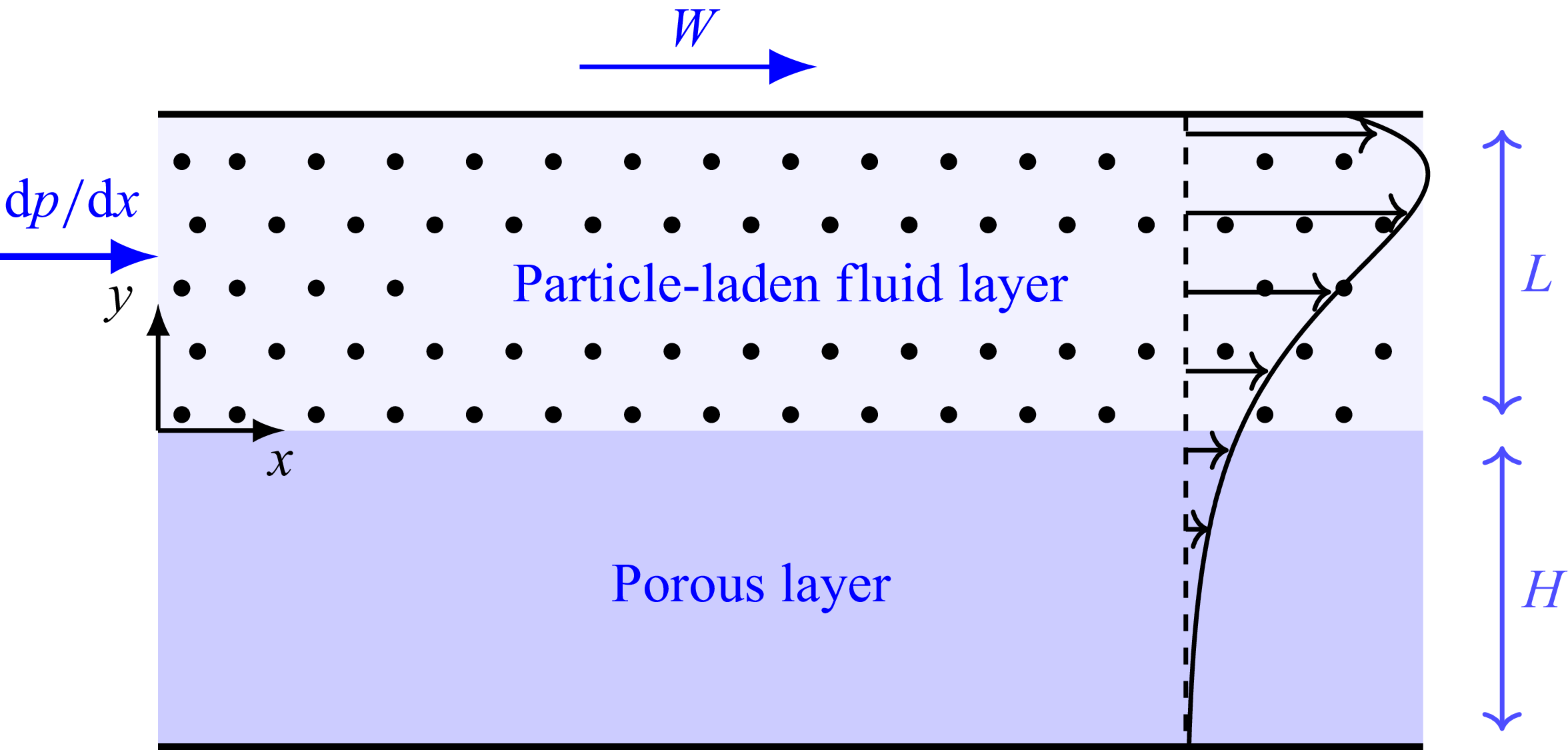
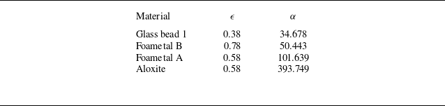

 α
α ϵ
ϵ τ
τ δ
δ W∗
W∗ ui
ui αδϵ
αδϵ τϵ
τϵ δ
δ W∗
W∗ δ
δ W∗
W∗ δ
δ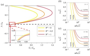
 W∗
W∗ ϵ
ϵ τ
τ δ
δ α
α ui
ui αδϵ
αδϵ τϵ
τϵ δ
δ W∗
W∗ δ
δ W∗
W∗ δ
δ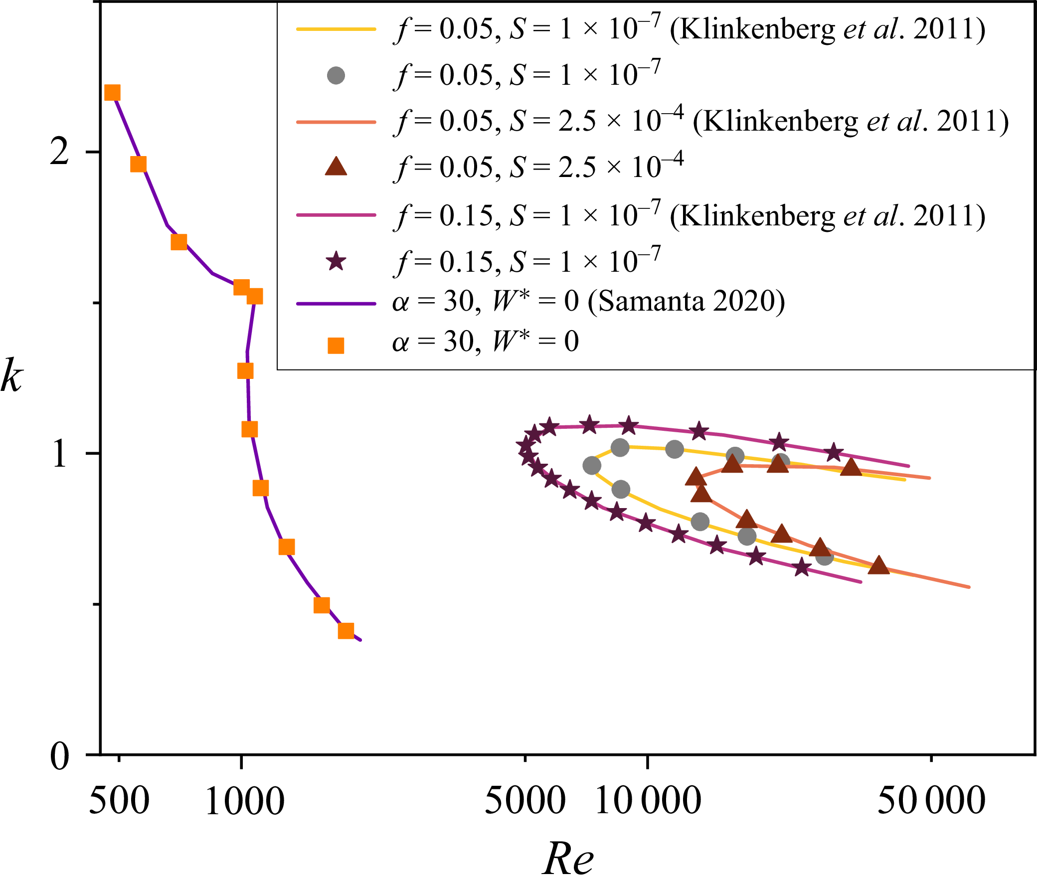

 α
α W∗=0
W∗=0 α
α S=1×10⁻⁷
 α
α S=5×10⁻⁵
 α
α S=2.5×10⁻⁴
 α
α S=1×10⁻⁷
 α
α S=5×10⁻⁵
 α
α S=2.5×10⁻⁴
 Re=1550
 k=2.7
k=2.7 α
α Re=6500
 k=2.18
 α
α τ
τ ϵ
ϵ δ
δ
 α
α W∗=0.5
 α
α S=1×10⁻⁷
 α
α S=5×10⁻⁵
 α
α S=2.5×10⁻⁴
 α
α S=1×10⁻⁷
 α
α S=5×10⁻⁵
 α
α S=2.5×10⁻⁴
 Re=1250
 k=2
k=2 α
α Re=7000
 k=1.38
 α
α τ
τ ϵ
ϵ δ
δ
 α
α α
α f
f W∗
W∗ Re
Re k
k α
α f
f W∗
W∗ Re
Re k
k α
α f
f S=5×10⁻⁵
 Re
Re k
k α
α f
f S=5×10⁻⁵
 Re
Re k
k τ
τ ϵ
ϵ δ
δ
 f
f S
S α
α α
α k
k Re
Re α
α k
k Re
Re α
α k
k Re
Re τ
τ ϵ
ϵ δ
δ
 S
S f
f α
α W∗
W∗ S=1×10⁻⁷
 S=5×10⁻⁵
 S=2.5×10⁻⁴
 τ
τ ϵ
ϵ δ
δ
 S=1×10⁻⁷
 W∗
W∗ S=2.5×10⁻⁴
 W∗
W∗ α
α f
f S=5×10⁻⁵
 W∗
W∗ f
f S=5×10⁻⁵
 α
α f
f S=5×10⁻⁵
 α
α ϵ
ϵ τ
τ δ
δ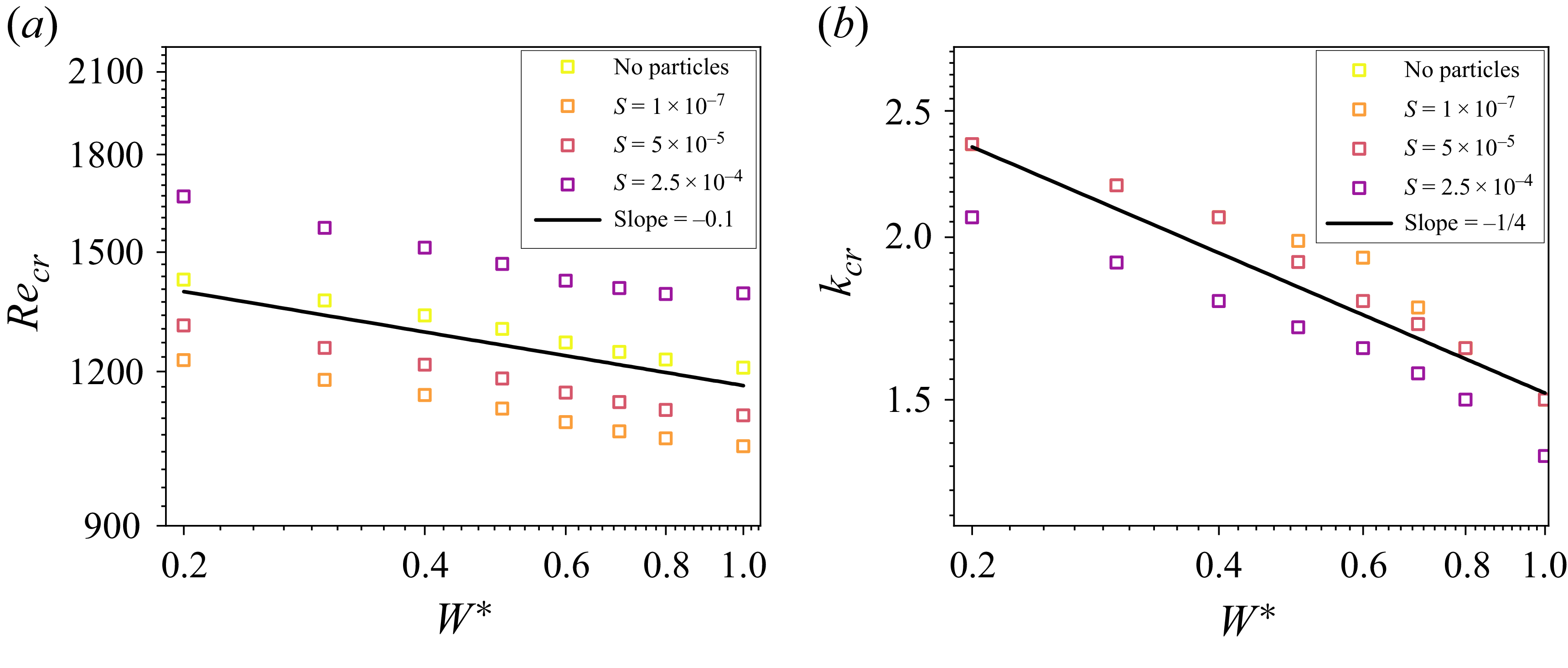
 S
S S
S f
f S=1×10⁻⁷
 f
f α
α ϵ
ϵ τ
τ δ
δ
 u
u v
v f
f S
S 2.5×10⁻⁴
 α
α W∗
W∗ α
α W∗
W∗ α
α W∗
W∗ α
α W∗
W∗ ϵ
ϵ τ
τ δ
δ
 S=1×10⁻⁷
 S=5×10⁻⁵
 S=2.5×10⁻⁴
 Re
Re k
k ϵ
ϵ τ
τ δ
δ
 α
α S=1×10⁻⁷
 S=5×10⁻⁵
 S=2.5×10⁻⁴
 Re
Re k
k ϵ
ϵ τ
τ δ
δ
 ϕ
ϕ ϕm
ϕm (x,y)
(x,y) α
α α=400
α=400 Recr
Recr kcr=1.88
 α=100
α=100 Recr
Recr kcr=2.6
 α=50
α=50 Recr
Recr kcr=2.8
 f=0.15
 S=5×10⁻⁵
 δ=1
δ=1 ϵ=0.6
ϵ=0.6 W∗=0
W∗=0 τ=0
τ=0
 Open access

