


1 Introduction
Experimental successes over the past decade have led to renewed interest in the stellarator as a viable path for fusion energy. The Helically Symmetric Experiment (HSX, Anderson et al. Reference Anderson, Almagri, Anderson, Peter, Talmadge and Shohet1995) demonstrated that a quasi-helically symmetric magnetic configuration (Boozer Reference Boozer1981) reduces neoclassical transport to levels below that of the equivalent tokamak (Canik et al. Reference Canik, Anderson, Anderson, Likin, Talmadge and Zhai2007). The large helical device (LHD) has achieved record length steady-state discharges (Yoshimura et al. Reference Yoshimura, Kubo, Shimozuma, Igami, Mutoh, Nakamura, Ohkubo, Notake, Takita and Kobayashi2005) and core ion temperatures in excess of 8 keV (Nagaoka et al. Reference Nagaoka, Takahashi, Murakami, Nakano, Takeiri, Tsuchiya, Osakabe, Ida, Yokoyama and Yoshinuma2015). Recently, the Wendelstein 7-X experiment reported some of the highest energy confinement times observed in stellarators (Dinklage et al. Reference Dinklage, Beidler, Helander, Fuchert, Maaßberg, Rahbarnia, Sunn Pedersen, Turkin, Wolf and Alonso2018). A defining feature of the stellarator is avoiding a reliance on plasma currents for confinement by providing the requisite rotational transform necessary for particle confinement through external shaping of the magnetic field. The resulting confining magnetic field is necessarily three-dimensional (Boozer Reference Boozer1998; Helander Reference Helander2014). While there are distinct advantages to this approach, such as the elimination of destructive magnetohydrodynamic instabilities and the ability to manipulate the magnetic geometry to target specific physics issues, using three-dimensional (3-D) magnetic fields increases complexity in both theory and experiment (Gates et al. Reference Gates, Anderson, Anderson, Zarnstorff, Spong, Weitzner, Neilson, Ruzic, Andruczyk and Harris2018). Paralleling the rise of interest in stellarators, computing capabilities have reached a level enabling comprehensive simulations of computationally challenging problems in a stellarator geometry, such as modelling turbulence with gyrokinetic codes (Xanthopoulos & Jenko Reference Xanthopoulos and Jenko2007; Baumgaertel et al. Reference Baumgaertel, Belli, Dorland, Guttenfelder, Hammett, Mikkelsen, Rewoldt, Tang and Xanthopoulos2011; Proll, Xanthopoulos & Helander Reference Proll, Xanthopoulos and Helander2013; Faber et al. Reference Faber, Pueschel, Proll, Xanthopoulos, Terry, Hegna, Weir, Likin and Talmadge2015; Xanthopoulos et al. Reference Xanthopoulos, Plunk, Zocco and Helander2016). In this work, gyrokinetic simulations are employed to describe the microturbulence properties of stellarators in the limit of small averaged magnetic shear.
A significant body of literature exists studying turbulence in toroidal geometries by means of gyrokinetic simulation in flux-tube simulation domains, see e.g. Dimits et al. (Reference Dimits, Williams, Byers and Cohen1996), Dorland et al. (Reference Dorland, Jenko, Kotschenreuther and Rogers2000), Jenko et al. (Reference Jenko, Dorland, Kotschenreuther and Rogers2000), Candy & Waltz (Reference Candy and Waltz2003), Sugama & Watanabe (Reference Sugama and Watanabe2006), Peeters et al. (Reference Peeters, Camenen, Casson, Hornsby, Snodin, Strintzi and Szepesi2009), Chen et al. (Reference Chen, Parker, Wan and Bravenec2013). A challenge to performing flux tube simulations for stellarators is that by design, global magnetic shear for many modern stellarators configurations is small. Magnetic shear tends to localize fluctuations, in tokamak core plasmas typically to the outboard midplane. In the absence of large global magnetic shear, mode localization is determined by the interplay of local shear and curvature, which is non-trivial for stellarators. This can manifest with modes that extend far along field lines or balloon in locations other than the outboard midplane (Merz Reference Merz2008; Faber et al. Reference Faber, Pueschel, Proll, Xanthopoulos, Terry, Hegna, Weir, Likin and Talmadge2015), adding significant complexity to the simulation and analysis of stellarator turbulence. Furthermore, the computational domain dimensions for flux tube simulations are inversely proportional to global magnetic shear, which can make flux-tube simulations for low-magnetic-shear stellarators comparatively expensive in the conventional formulation (Beer, Cowley & Hammett Reference Beer, Cowley and Hammett1995). One method to reduce the computational cost is to approximate a low-magnetic-shear flux tube with a zero-magnetic-shear domain, where the domain dimensions are independent of global magnetic shear and can be specified to reasonable values.
In this paper, a gyrokinetic study of the low-magnetic-shear stellarator HSX demonstrates that properly resolving parallel correlation lengths with extended simulation domains is crucial for accurate theoretical predictions. Turbulence is studied in the ‘bean’ flux tube of the quasi-helically symmetric (QHS) configuration of HSX, used previously in Faber et al. (Reference Faber, Pueschel, Proll, Xanthopoulos, Terry, Hegna, Weir, Likin and Talmadge2015) and shown for different geometry elements in figure 1. The rotational transform ![]() for HSX is constrained such that
for HSX is constrained such that ![]() and
and ![]() and at the half-radius in the toroidal flux coordinate
and at the half-radius in the toroidal flux coordinate
 $\unicode[STIX]{x1D6F9}/\unicode[STIX]{x1D6F9}_{\text{edge}}=0.5$
, where
$\unicode[STIX]{x1D6F9}/\unicode[STIX]{x1D6F9}_{\text{edge}}=0.5$
, where
 $\unicode[STIX]{x1D713}_{\text{edge}}$
is the toroidal flux at the last closed flux surface. For the focus of this analysis, the global magnetic shear is
$\unicode[STIX]{x1D713}_{\text{edge}}$
is the toroidal flux at the last closed flux surface. For the focus of this analysis, the global magnetic shear is
 ${\hat{s}}\approx -0.046$
. Modes that extend far along field lines tend to have subdominant growth rates with growth rates
${\hat{s}}\approx -0.046$
. Modes that extend far along field lines tend to have subdominant growth rates with growth rates
 $0<\unicode[STIX]{x1D6FE}<\unicode[STIX]{x1D6FE}_{\text{max}}$
and usually do not merit detailed investigation. For HSX geometry these modes prove essential to determining the final turbulent state. In particular, when the zero-shear computational technique was used with an insufficiently large parallel simulation domain, the resulting simulations showed no flux, in direct contradiction with finite-shear simulations. Using parallel simulation domains comprised of multiple poloidal turns resolves parallel correlation lengths and leads to agreement between finite-shear and zero-shear simulations. It is observed that despite the extended modes being linearly stable for the larger parallel simulation domains, they play a prominent role in the nonlinear dynamics of the turbulence, acting as both an energy drive and an important nonlinear energy transfer channel at long wavelengths. Fundamentally, the results shown in the present paper can be seen as part of a larger picture, where subdominant eigenmodes and stable eigenmodes with
$0<\unicode[STIX]{x1D6FE}<\unicode[STIX]{x1D6FE}_{\text{max}}$
and usually do not merit detailed investigation. For HSX geometry these modes prove essential to determining the final turbulent state. In particular, when the zero-shear computational technique was used with an insufficiently large parallel simulation domain, the resulting simulations showed no flux, in direct contradiction with finite-shear simulations. Using parallel simulation domains comprised of multiple poloidal turns resolves parallel correlation lengths and leads to agreement between finite-shear and zero-shear simulations. It is observed that despite the extended modes being linearly stable for the larger parallel simulation domains, they play a prominent role in the nonlinear dynamics of the turbulence, acting as both an energy drive and an important nonlinear energy transfer channel at long wavelengths. Fundamentally, the results shown in the present paper can be seen as part of a larger picture, where subdominant eigenmodes and stable eigenmodes with
 $\unicode[STIX]{x1D6FE}<0$
have a significant impact on the nonlinear state (Terry, Baver & Gupta Reference Terry, Baver and Gupta2006; Hatch et al.
Reference Hatch, Terry, Jenko, Merz and Nevins2011a
,Reference Hatch, Terry, Jenko, Merz, Pueschel, Nevins and Wang
b
; Pueschel et al.
Reference Pueschel, Faber, Citrin, Hegna, Terry and Hatch2016). This should motivate the consideration of such modes in the design of reduced models.
$\unicode[STIX]{x1D6FE}<0$
have a significant impact on the nonlinear state (Terry, Baver & Gupta Reference Terry, Baver and Gupta2006; Hatch et al.
Reference Hatch, Terry, Jenko, Merz and Nevins2011a
,Reference Hatch, Terry, Jenko, Merz, Pueschel, Nevins and Wang
b
; Pueschel et al.
Reference Pueschel, Faber, Citrin, Hegna, Terry and Hatch2016). This should motivate the consideration of such modes in the design of reduced models.
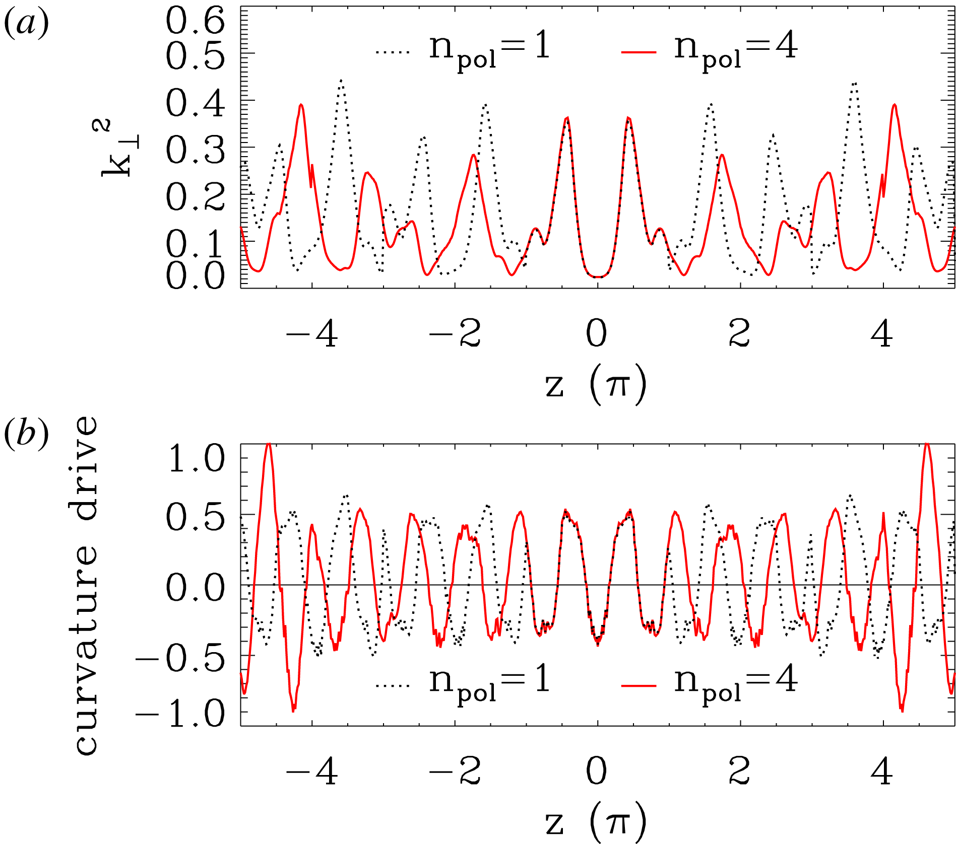
Comparison of HSX geometry terms for a flux tube constructed from one poloidal turn (black) and four poloidal turns (red solid lines). The FLR term, defined by (2.10), is shown in (a), while the curvature drive, defined by (2.11), is shown in (b). Both quantities are plotted as functions of the parallel coordinate.
The remainder of the paper is organized as follows. Section 2 discusses flux-tube simulations and the necessary considerations to resolve parallel correlation lengths in low-magnetic-shear stellarators. Section 3 presents linear eigenvalue calculations for both strongly driven trapped electron modes (TEMs) and ion temperature gradient (ITG) modes in HSX. Also discussed in § 3 is the zero-magnetic-shear simulation technique and the importance of properly resolving parallel correlation lengths for accurate simulations. Nonlinear results are presented in § 4, focusing on the role subdominant, extended modes play in the dynamics of nonlinear simulations. Concluding remarks are presented in § 5.
2 Geometry considerations at low magnetic shear
2.1 Flux-tube geometry
Gyrokinetic simulations of local plasma turbulence utilize the flux-tube approach (Beer et al.
Reference Beer, Cowley and Hammett1995), where the gyrokinetic equations are solved in a small domain around a magnetic field line. This approach takes advantage of the anisotropic nature of plasma turbulence, where perpendicular wavelengths of fluctuations are generally much smaller than parallel wavelengths,
 $k_{\Vert }\ll k_{\bot }$
. Only a small domain perpendicular to the field line, of the order of a few perpendicular correlation lengths, need be simulated with periodic boundary conditions. The scale
$k_{\Vert }\ll k_{\bot }$
. Only a small domain perpendicular to the field line, of the order of a few perpendicular correlation lengths, need be simulated with periodic boundary conditions. The scale
 $L_{\text{eq}}$
of perpendicular variations of background quantities such as the equilibrium magnetic field is assumed to be much larger than turbulent correlations lengths
$L_{\text{eq}}$
of perpendicular variations of background quantities such as the equilibrium magnetic field is assumed to be much larger than turbulent correlations lengths
 $\unicode[STIX]{x1D706}_{\text{turb}}$
. Equilibrium quantities are then expanded to first order in the perpendicular direction around the centre of the simulation domain while still incorporating non-trivial dependence along the parallel field-line coordinate.
$\unicode[STIX]{x1D706}_{\text{turb}}$
. Equilibrium quantities are then expanded to first order in the perpendicular direction around the centre of the simulation domain while still incorporating non-trivial dependence along the parallel field-line coordinate.
The flux-tube approach is related to the ballooning transformation formulated for axisymmetric geometries (Connor, Hastie & Taylor Reference Connor, Hastie and Taylor1978, Reference Connor, Hastie and Taylor1979) and subsequently extended to general three-dimensional systems (Dewar & Glasser Reference Dewar and Glasser1983), which transforms a multi-dimensional eigenvalue calculation into a sequence of one-dimensional eigenvalue equations along field lines. This transformation is facilitated by the assumption
 $k_{\Vert }\ll k_{\bot }$
for ballooning modes, allowing one to assume a Wentzel–Kramers–Brillouin-like solution where the slow scale only appears in the mode amplitude:
$k_{\Vert }\ll k_{\bot }$
for ballooning modes, allowing one to assume a Wentzel–Kramers–Brillouin-like solution where the slow scale only appears in the mode amplitude:
 $\unicode[STIX]{x1D709}(\boldsymbol{x},t)=\hat{\unicode[STIX]{x1D709}}(\boldsymbol{x},\unicode[STIX]{x1D716})\exp (\text{i}S(\boldsymbol{x})/\unicode[STIX]{x1D716}-\text{i}\unicode[STIX]{x1D714}t)$
, where
$\unicode[STIX]{x1D709}(\boldsymbol{x},t)=\hat{\unicode[STIX]{x1D709}}(\boldsymbol{x},\unicode[STIX]{x1D716})\exp (\text{i}S(\boldsymbol{x})/\unicode[STIX]{x1D716}-\text{i}\unicode[STIX]{x1D714}t)$
, where
 $\unicode[STIX]{x1D709}$
is the plasma displacement.
$\unicode[STIX]{x1D709}$
is the plasma displacement.
 $\unicode[STIX]{x1D716}\ll 1$
is an expansion parameter and denotes the rapid variation of the wave phase perpendicular to the magnetic field line. At lowest order in
$\unicode[STIX]{x1D716}\ll 1$
is an expansion parameter and denotes the rapid variation of the wave phase perpendicular to the magnetic field line. At lowest order in
 $\unicode[STIX]{x1D716}$
, the instabilities are approximately incompressible,
$\unicode[STIX]{x1D716}$
, the instabilities are approximately incompressible,
 $\unicode[STIX]{x1D735}\boldsymbol{\cdot }\unicode[STIX]{x1D743}\approx (\text{i}\unicode[STIX]{x1D735}S(\boldsymbol{x})/\unicode[STIX]{x1D716})\boldsymbol{\cdot }\unicode[STIX]{x1D743}=0$
. We can identify
$\unicode[STIX]{x1D735}\boldsymbol{\cdot }\unicode[STIX]{x1D743}\approx (\text{i}\unicode[STIX]{x1D735}S(\boldsymbol{x})/\unicode[STIX]{x1D716})\boldsymbol{\cdot }\unicode[STIX]{x1D743}=0$
. We can identify
 $\unicode[STIX]{x1D735}S(\boldsymbol{x})$
as the wavevector
$\unicode[STIX]{x1D735}S(\boldsymbol{x})$
as the wavevector
 $\boldsymbol{k}$
. Requiring the displacement at lowest order to be perpendicular to the magnetic field gives
$\boldsymbol{k}$
. Requiring the displacement at lowest order to be perpendicular to the magnetic field gives
 $\boldsymbol{k}_{\bot }\boldsymbol{\cdot }\boldsymbol{B}=0$
. We may write the magnetic field in Clebsch form,
$\boldsymbol{k}_{\bot }\boldsymbol{\cdot }\boldsymbol{B}=0$
. We may write the magnetic field in Clebsch form,
 $$\begin{eqnarray}\boldsymbol{B}=\unicode[STIX]{x1D735}\unicode[STIX]{x1D713}\times \unicode[STIX]{x1D735}\unicode[STIX]{x1D6FC},\end{eqnarray}$$
where
 $\unicode[STIX]{x1D713}$
is the poloidal magnetic flux function and
$\unicode[STIX]{x1D713}$
is the poloidal magnetic flux function and
 $\unicode[STIX]{x1D6FC}=q(\unicode[STIX]{x1D713})\unicode[STIX]{x1D703}-\unicode[STIX]{x1D701}$
is the field-line label defined in terms of the straight field-line poloidal and toroidal angles
$\unicode[STIX]{x1D6FC}=q(\unicode[STIX]{x1D713})\unicode[STIX]{x1D703}-\unicode[STIX]{x1D701}$
is the field-line label defined in terms of the straight field-line poloidal and toroidal angles
 $\unicode[STIX]{x1D703}$
and
$\unicode[STIX]{x1D703}$
and
 $\unicode[STIX]{x1D701}$
, respectively, and
$\unicode[STIX]{x1D701}$
, respectively, and
 $q(\unicode[STIX]{x1D713})$
is the safety factor. The condition
$q(\unicode[STIX]{x1D713})$
is the safety factor. The condition
 $\boldsymbol{k}_{\bot }\boldsymbol{\cdot }\boldsymbol{B}=0$
implies
$\boldsymbol{k}_{\bot }\boldsymbol{\cdot }\boldsymbol{B}=0$
implies
 $S(\boldsymbol{x})$
is a function of
$S(\boldsymbol{x})$
is a function of
 $(\unicode[STIX]{x1D713},\unicode[STIX]{x1D6FC})$
alone, yielding an instructive form for
$(\unicode[STIX]{x1D713},\unicode[STIX]{x1D6FC})$
alone, yielding an instructive form for
 $\boldsymbol{k}_{\bot }$
:
$\boldsymbol{k}_{\bot }$
:
 $$\begin{eqnarray}\boldsymbol{k}_{\bot }=k_{\unicode[STIX]{x1D6FC}}[q\unicode[STIX]{x1D735}\unicode[STIX]{x1D703}-\unicode[STIX]{x1D735}\unicode[STIX]{x1D701}+q^{\prime }(\unicode[STIX]{x1D703}+\unicode[STIX]{x1D703}_{k})\unicode[STIX]{x1D735}\unicode[STIX]{x1D713}].\end{eqnarray}$$
Here,
 $q^{\prime }=\text{d}q/\text{d}\unicode[STIX]{x1D713}$
is the flux-tube-averaged global magnetic shear and
$q^{\prime }=\text{d}q/\text{d}\unicode[STIX]{x1D713}$
is the flux-tube-averaged global magnetic shear and
 $\unicode[STIX]{x1D703}_{k}=k_{\unicode[STIX]{x1D713}}/q^{\prime }k_{\unicode[STIX]{x1D6FC}}$
is the ballooning angle. This implies that radial variations (finite-
$\unicode[STIX]{x1D703}_{k}=k_{\unicode[STIX]{x1D713}}/q^{\prime }k_{\unicode[STIX]{x1D6FC}}$
is the ballooning angle. This implies that radial variations (finite-
 $k_{\unicode[STIX]{x1D713}}$
effects) are transformed by global magnetic shear into a dependence along the field line. Furthermore, it is easy to see that (2.2) is invariant under the substitution
$k_{\unicode[STIX]{x1D713}}$
effects) are transformed by global magnetic shear into a dependence along the field line. Furthermore, it is easy to see that (2.2) is invariant under the substitution
 $\unicode[STIX]{x1D703}\rightarrow 2\unicode[STIX]{x03C0}M$
,
$\unicode[STIX]{x1D703}\rightarrow 2\unicode[STIX]{x03C0}M$
,
 $\unicode[STIX]{x1D703}_{k}\rightarrow -2\unicode[STIX]{x03C0}M$
for some integer
$\unicode[STIX]{x1D703}_{k}\rightarrow -2\unicode[STIX]{x03C0}M$
for some integer
 $M$
. Thus, in principle, one may compute effects for increasing
$M$
. Thus, in principle, one may compute effects for increasing
 $\unicode[STIX]{x1D703}$
by considering the geometry from a limited range of
$\unicode[STIX]{x1D703}$
by considering the geometry from a limited range of
 $\unicode[STIX]{x1D703}$
, say
$\unicode[STIX]{x1D703}$
, say
 $\unicode[STIX]{x1D703}\in (-\unicode[STIX]{x03C0},\unicode[STIX]{x03C0})$
and incrementing
$\unicode[STIX]{x1D703}\in (-\unicode[STIX]{x03C0},\unicode[STIX]{x03C0})$
and incrementing
 $k_{\unicode[STIX]{x1D713}}\rightarrow -2\unicode[STIX]{x03C0}Mq^{\prime }k_{\unicode[STIX]{x1D6FC}}$
for integer
$k_{\unicode[STIX]{x1D713}}\rightarrow -2\unicode[STIX]{x03C0}Mq^{\prime }k_{\unicode[STIX]{x1D6FC}}$
for integer
 $M$
.
$M$
.
The flux-tube simulation domain is defined in straight field-line (SFL) coordinates
 $(\unicode[STIX]{x1D713},\unicode[STIX]{x1D6FC},z)$
. Depending on whether one chooses
$(\unicode[STIX]{x1D713},\unicode[STIX]{x1D6FC},z)$
. Depending on whether one chooses
 $\unicode[STIX]{x1D6FC}=q\unicode[STIX]{x1D703}-\unicode[STIX]{x1D701}$
or
$\unicode[STIX]{x1D6FC}=q\unicode[STIX]{x1D703}-\unicode[STIX]{x1D701}$
or ![]()
 $\unicode[STIX]{x1D713}$
is the poloidal or toroidal flux label, respectively, and the rotational transform
$\unicode[STIX]{x1D713}$
is the poloidal or toroidal flux label, respectively, and the rotational transform ![]() is related to
is related to
 $q$
by
$q$
by ![]() For subsequent discussion and to be consistent with the formalism employed by the gyrokinetic code Gene (Jenko et al.
Reference Jenko, Dorland, Kotschenreuther and Rogers2000), we will choose
For subsequent discussion and to be consistent with the formalism employed by the gyrokinetic code Gene (Jenko et al.
Reference Jenko, Dorland, Kotschenreuther and Rogers2000), we will choose
 $\unicode[STIX]{x1D713}$
to be the poloidal flux and
$\unicode[STIX]{x1D713}$
to be the poloidal flux and
 $\unicode[STIX]{x1D6FC}=q(\unicode[STIX]{x1D713})\unicode[STIX]{x1D703}-\unicode[STIX]{x1D701}$
. The parallel coordinate
$\unicode[STIX]{x1D6FC}=q(\unicode[STIX]{x1D713})\unicode[STIX]{x1D703}-\unicode[STIX]{x1D701}$
. The parallel coordinate
 $z$
is chosen to be identical to the straight field-line poloidal angle
$z$
is chosen to be identical to the straight field-line poloidal angle
 $\unicode[STIX]{x1D703}$
. In these coordinates, the flux-tube simulation domain is defined to be a small rectangular domain centred around
$\unicode[STIX]{x1D703}$
. In these coordinates, the flux-tube simulation domain is defined to be a small rectangular domain centred around
 $\unicode[STIX]{x1D713}_{0}$
and
$\unicode[STIX]{x1D713}_{0}$
and
 $\unicode[STIX]{x1D6FC}_{0}$
in SFL coordinates, given by
$\unicode[STIX]{x1D6FC}_{0}$
in SFL coordinates, given by
 $$\begin{eqnarray}\left.\begin{array}{@{}c@{}}\unicode[STIX]{x1D713}_{0}-\unicode[STIX]{x0394}\unicode[STIX]{x1D713}\leqslant \unicode[STIX]{x1D713}<\unicode[STIX]{x1D713}_{0}+\unicode[STIX]{x0394}\unicode[STIX]{x1D713},\\ \unicode[STIX]{x1D6FC}_{0}-\unicode[STIX]{x0394}\unicode[STIX]{x1D6FC}\leqslant \unicode[STIX]{x1D6FC}<\unicode[STIX]{x1D6FC}_{0}+\unicode[STIX]{x0394}\unicode[STIX]{x1D6FC},\\ -z_{0}/2\leqslant z<z_{0}/2.\end{array}\right\}\end{eqnarray}$$
The flux-tube approach assumes periodic boundary conditions in the perpendicular directions, however this is an assumption of statistical, not physical, periodicity; that is, the statistical properties of the fluctuations at
 $\unicode[STIX]{x1D713}$
and
$\unicode[STIX]{x1D713}$
and
 $\unicode[STIX]{x1D713}+2\unicode[STIX]{x0394}\unicode[STIX]{x1D713}$
while holding
$\unicode[STIX]{x1D713}+2\unicode[STIX]{x0394}\unicode[STIX]{x1D713}$
while holding
 $\unicode[STIX]{x1D6FC}$
fixed, or at
$\unicode[STIX]{x1D6FC}$
fixed, or at
 $\unicode[STIX]{x1D6FC}$
and
$\unicode[STIX]{x1D6FC}$
and
 $\unicode[STIX]{x1D6FC}+2\unicode[STIX]{x0394}\unicode[STIX]{x1D6FC}$
while holding
$\unicode[STIX]{x1D6FC}+2\unicode[STIX]{x0394}\unicode[STIX]{x1D6FC}$
while holding
 $\unicode[STIX]{x1D713}$
fixed, are the same. Provided the domain dimensions are larger than physical correlation lengths of the fluctuations, which are typically of the order of tens of gyroradii in the radial direction, periodic boundary conditions are an efficient means to represent turbulent eddies entering and leaving the domain. A benefit of prescribing periodic perpendicular boundary conditions is that quantities can be decomposed in a Fourier basis in
$\unicode[STIX]{x1D713}$
fixed, are the same. Provided the domain dimensions are larger than physical correlation lengths of the fluctuations, which are typically of the order of tens of gyroradii in the radial direction, periodic boundary conditions are an efficient means to represent turbulent eddies entering and leaving the domain. A benefit of prescribing periodic perpendicular boundary conditions is that quantities can be decomposed in a Fourier basis in
 $\unicode[STIX]{x1D713}$
and
$\unicode[STIX]{x1D713}$
and
 $\unicode[STIX]{x1D6FC}$
:
$\unicode[STIX]{x1D6FC}$
:
 $$\begin{eqnarray}f(\unicode[STIX]{x1D713},\unicode[STIX]{x1D6FC},z,t)=\mathop{\sum }_{m=-\infty }^{\infty }\mathop{\sum }_{n=-\infty }^{\infty }\hat{f}_{m,n}(z,t)\exp [\text{i}m\unicode[STIX]{x03C0}(\unicode[STIX]{x1D713}-\unicode[STIX]{x1D713}_{0})/\unicode[STIX]{x0394}\unicode[STIX]{x1D713}+\text{i}n\unicode[STIX]{x03C0}(\unicode[STIX]{x1D6FC}-\unicode[STIX]{x1D6FC}_{0})/\unicode[STIX]{x0394}\unicode[STIX]{x1D6FC}],\end{eqnarray}$$
for each physical quantity
 $f$
.
$f$
.
A more subtle treatment is required for the parallel boundary condition as enforcing strictly periodic boundary conditions in the parallel direction,
 $f(\unicode[STIX]{x1D713},\unicode[STIX]{x1D6FC},-z_{0},t)=f(\unicode[STIX]{x1D713},\unicode[STIX]{x1D6FC},z_{0},t)$
, leads to rational field lines, which is inaccurate for toroidal magnetic confinement configurations. Like the perpendicular boundary conditions, the parallel boundary condition should be an expression of the statistical properties of the fluctuations, which physically should be statistically invariant at the same poloidal angle along the field line. In order for this to successfully be satisfied, the parallel simulation domain must be longer than the parallel correlation length of the fluctuation. This is accomplished by applying periodic boundary conditions at different
$f(\unicode[STIX]{x1D713},\unicode[STIX]{x1D6FC},-z_{0},t)=f(\unicode[STIX]{x1D713},\unicode[STIX]{x1D6FC},z_{0},t)$
, leads to rational field lines, which is inaccurate for toroidal magnetic confinement configurations. Like the perpendicular boundary conditions, the parallel boundary condition should be an expression of the statistical properties of the fluctuations, which physically should be statistically invariant at the same poloidal angle along the field line. In order for this to successfully be satisfied, the parallel simulation domain must be longer than the parallel correlation length of the fluctuation. This is accomplished by applying periodic boundary conditions at different
 $\unicode[STIX]{x1D703}$
values, while holding
$\unicode[STIX]{x1D703}$
values, while holding
 $\unicode[STIX]{x1D713}$
and
$\unicode[STIX]{x1D713}$
and
 $\unicode[STIX]{x1D701}$
fixed, rather than holding
$\unicode[STIX]{x1D701}$
fixed, rather than holding
 $\unicode[STIX]{x1D713}$
and
$\unicode[STIX]{x1D713}$
and
 $\unicode[STIX]{x1D6FC}$
fixed, which leads to every field line being rational. The detailed derivation of the parallel boundary condition is given in appendix A, giving the final form as
$\unicode[STIX]{x1D6FC}$
fixed, which leads to every field line being rational. The detailed derivation of the parallel boundary condition is given in appendix A, giving the final form as
 $$\begin{eqnarray}\displaystyle & \hat{f}_{m-\unicode[STIX]{x1D6FF}m,n}(\unicode[STIX]{x1D703}+2\unicode[STIX]{x03C0}N,t)C_{n}=\hat{f}_{m,n}(\unicode[STIX]{x1D703},t), & \displaystyle\end{eqnarray}$$
 $$\begin{eqnarray}\displaystyle & \unicode[STIX]{x1D6FF}m=nM,\quad M=2\unicode[STIX]{x03C0}Nq^{\prime }{\displaystyle \frac{\unicode[STIX]{x0394}\unicode[STIX]{x1D713}}{\unicode[STIX]{x0394}\unicode[STIX]{x1D6FC}}}. & \displaystyle\end{eqnarray}$$
Equation (2.5) expresses that the amplitude of a mode with index
 $m$
at one end of the parallel simulation domain is coupled to a mode with index
$m$
at one end of the parallel simulation domain is coupled to a mode with index
 $m-\unicode[STIX]{x1D6FF}m$
at the other end of the parallel simulation domain, with the coupling dependent on the global magnetic shear,
$m-\unicode[STIX]{x1D6FF}m$
at the other end of the parallel simulation domain, with the coupling dependent on the global magnetic shear,
 $q^{\prime }$
. Equation (2.5) contains the phase factor
$q^{\prime }$
. Equation (2.5) contains the phase factor
 $C_{n}=\exp (\text{i}2\unicode[STIX]{x03C0}Nnq_{0}/\unicode[STIX]{x0394}\unicode[STIX]{x1D6FC})$
. For further use in Gene, the following field-aligned coordinate system is used:
$C_{n}=\exp (\text{i}2\unicode[STIX]{x03C0}Nnq_{0}/\unicode[STIX]{x0394}\unicode[STIX]{x1D6FC})$
. For further use in Gene, the following field-aligned coordinate system is used:
 $$\begin{eqnarray}x=\frac{q_{0}}{B_{0}r_{0}}(\unicode[STIX]{x1D713}-\unicode[STIX]{x1D713}_{0}),\quad y=\frac{r_{0}}{q_{0}}(\unicode[STIX]{x1D6FC}-\unicode[STIX]{x1D6FC}_{0}),\quad z=\unicode[STIX]{x1D703},\end{eqnarray}$$
where
 $r_{0}$
is the geometrical radius of the magnetic surface at the centre of the simulation domain,
$r_{0}$
is the geometrical radius of the magnetic surface at the centre of the simulation domain,
 $\unicode[STIX]{x1D713}_{0}=\unicode[STIX]{x1D713}(r_{0})$
, with
$\unicode[STIX]{x1D713}_{0}=\unicode[STIX]{x1D713}(r_{0})$
, with
 $q_{0}$
the safety factor,
$q_{0}$
the safety factor,
 $B_{0}$
the magnetic field and
$B_{0}$
the magnetic field and
 $\unicode[STIX]{x1D6FC}_{0}$
the field-line label at the centre of the simulation domain. Similarly, the radial wavenumber
$\unicode[STIX]{x1D6FC}_{0}$
the field-line label at the centre of the simulation domain. Similarly, the radial wavenumber
 $k_{\unicode[STIX]{x1D713}}$
and binormal wavenumber
$k_{\unicode[STIX]{x1D713}}$
and binormal wavenumber
 $k_{\unicode[STIX]{x1D6FC}}$
can be redefined as
$k_{\unicode[STIX]{x1D6FC}}$
can be redefined as
 $$\begin{eqnarray}k_{x}=\frac{m\unicode[STIX]{x03C0}B_{0}r_{0}}{q_{0}\unicode[STIX]{x0394}\unicode[STIX]{x1D713}},\quad k_{y}=\frac{n\unicode[STIX]{x03C0}q_{0}}{r_{0}\unicode[STIX]{x0394}\unicode[STIX]{x1D6FC}}.\end{eqnarray}$$
Finally, the perpendicular coordinates
 $x$
and
$x$
and
 $y$
are normalized to a reference gyroradius length scale:
$y$
are normalized to a reference gyroradius length scale:
 $\hat{x}=x/\unicode[STIX]{x1D70C}_{\text{ref}}$
,
$\hat{x}=x/\unicode[STIX]{x1D70C}_{\text{ref}}$
,
 ${\hat{y}}=y/\unicode[STIX]{x1D70C}_{\text{ref}}$
, yielding
${\hat{y}}=y/\unicode[STIX]{x1D70C}_{\text{ref}}$
, yielding
 $\hat{k}_{x}=k_{x}\unicode[STIX]{x1D70C}_{\text{ref}}$
and
$\hat{k}_{x}=k_{x}\unicode[STIX]{x1D70C}_{\text{ref}}$
and
 $\hat{k}_{y}=k_{y}\unicode[STIX]{x1D70C}_{\text{ref}}$
. For discussion of the following results, the normalized coordinates will be used, however the over hat symbols will be dropped. The local magnetic shear is defined by the vector relation
$\hat{k}_{y}=k_{y}\unicode[STIX]{x1D70C}_{\text{ref}}$
. For discussion of the following results, the normalized coordinates will be used, however the over hat symbols will be dropped. The local magnetic shear is defined by the vector relation
 $$\begin{eqnarray}s_{\text{loc}}(z)=\hat{\boldsymbol{b}}(z)\times \unicode[STIX]{x1D735}\hat{\boldsymbol{n}}(z)\boldsymbol{\cdot }\unicode[STIX]{x1D735}\times (\hat{\boldsymbol{b}}(z)\times \unicode[STIX]{x1D735}\hat{\boldsymbol{n}}(z)),\end{eqnarray}$$
where
 $\hat{\boldsymbol{b}}$
is the unit vector in the direction of the magnetic field and
$\hat{\boldsymbol{b}}$
is the unit vector in the direction of the magnetic field and
 $\hat{\boldsymbol{n}}=\unicode[STIX]{x1D735}\unicode[STIX]{x1D713}(z)/|\unicode[STIX]{x1D735}\unicode[STIX]{x1D713}(z)|$
. Due to the complicated magnetic field structures in stellarators, equation (2.9) has non-trivial dependence along field lines. The global magnetic shear is defined as the flux surface average of (2.9) and can be shown to be equal to
$\hat{\boldsymbol{n}}=\unicode[STIX]{x1D735}\unicode[STIX]{x1D713}(z)/|\unicode[STIX]{x1D735}\unicode[STIX]{x1D713}(z)|$
. Due to the complicated magnetic field structures in stellarators, equation (2.9) has non-trivial dependence along field lines. The global magnetic shear is defined as the flux surface average of (2.9) and can be shown to be equal to
 ${\hat{s}}=(r_{0}/q_{0})\,\text{d}q/\text{d}r$
.
${\hat{s}}=(r_{0}/q_{0})\,\text{d}q/\text{d}r$
.
2.2 Parallel correlations
Drift-wave instabilities in flux-tube simulations typically have ballooning nature, thus
 $\boldsymbol{k}_{\bot }$
takes on the same form as (2.2). Instead of solving the gyrokinetic equations over a long parallel domain, one may make use of this form of
$\boldsymbol{k}_{\bot }$
takes on the same form as (2.2). Instead of solving the gyrokinetic equations over a long parallel domain, one may make use of this form of
 $\boldsymbol{k}_{\bot }$
and the parallel boundary condition to construct fluctuations that extend along field lines by adding more radial modes, which takes advantage of fast Fourier transform techniques (Dorland et al.
Reference Dorland, Jenko, Kotschenreuther and Rogers2000; Jenko et al.
Reference Jenko, Dorland, Kotschenreuther and Rogers2000; Peeters et al.
Reference Peeters, Camenen, Casson, Hornsby, Snodin, Strintzi and Szepesi2009). The approach is well suited for axisymmetric configurations. After one poloidal turn (
$\boldsymbol{k}_{\bot }$
and the parallel boundary condition to construct fluctuations that extend along field lines by adding more radial modes, which takes advantage of fast Fourier transform techniques (Dorland et al.
Reference Dorland, Jenko, Kotschenreuther and Rogers2000; Jenko et al.
Reference Jenko, Dorland, Kotschenreuther and Rogers2000; Peeters et al.
Reference Peeters, Camenen, Casson, Hornsby, Snodin, Strintzi and Szepesi2009). The approach is well suited for axisymmetric configurations. After one poloidal turn (
 $\unicode[STIX]{x1D703}\rightarrow \unicode[STIX]{x1D703}+2\unicode[STIX]{x03C0}$
), all geometric quantities are periodic, even though the flux-tube ends generally lie at different
$\unicode[STIX]{x1D703}\rightarrow \unicode[STIX]{x1D703}+2\unicode[STIX]{x03C0}$
), all geometric quantities are periodic, even though the flux-tube ends generally lie at different
 $\unicode[STIX]{x1D701}$
values. This is guaranteed by axisymmetry, as
$\unicode[STIX]{x1D701}$
values. This is guaranteed by axisymmetry, as
 $\unicode[STIX]{x1D701}$
is an ignorable coordinate and the flux tube is parameterized only by
$\unicode[STIX]{x1D701}$
is an ignorable coordinate and the flux tube is parameterized only by
 $\unicode[STIX]{x1D703}$
. Thus, one may use the geometric data from one poloidal turn and ‘build’ an extended flux tube by adding more radial modes. A geometrically accurate computational domain can then be constructed for fluctuations that have arbitrarily large parallel correlation lengths, as one may always add a sufficient number of radial modes to resolve parallel scales.
$\unicode[STIX]{x1D703}$
. Thus, one may use the geometric data from one poloidal turn and ‘build’ an extended flux tube by adding more radial modes. A geometrically accurate computational domain can then be constructed for fluctuations that have arbitrarily large parallel correlation lengths, as one may always add a sufficient number of radial modes to resolve parallel scales.
While often yielding reasonably accurate results, this procedure is formally incorrect for most stellarator simulations. In general, geometric quantities for stellarators are not periodic after one poloidal turn, which can have serious consequences for stellarator flux-tube simulations. As a fluctuation extends along a field line in a stellarator, it samples different geometry depending on the field-line label. The exact geometry may be important in setting the physical parallel correlation length. Due to the complicated interplay of magnetic trapping regions, curvature drive and local magnetic shear, it has been observed that drift-wave instabilities in stellarators may be most unstable in regions away from
 $\unicode[STIX]{x1D703}_{k}=0$
at the outboard midplane (Merz Reference Merz2008; Faber et al.
Reference Faber, Pueschel, Proll, Xanthopoulos, Terry, Hegna, Weir, Likin and Talmadge2015), where one might naively expect the fastest-growing instabilities are centred. This is readily apparent in low-global-magnetic-shear stellarators, such as HSX, where fluctuations have been observed to extend to
$\unicode[STIX]{x1D703}_{k}=0$
at the outboard midplane (Merz Reference Merz2008; Faber et al.
Reference Faber, Pueschel, Proll, Xanthopoulos, Terry, Hegna, Weir, Likin and Talmadge2015), where one might naively expect the fastest-growing instabilities are centred. This is readily apparent in low-global-magnetic-shear stellarators, such as HSX, where fluctuations have been observed to extend to
 $|\unicode[STIX]{x1D703}|\geqslant 30\unicode[STIX]{x03C0}$
or peak well away from
$|\unicode[STIX]{x1D703}|\geqslant 30\unicode[STIX]{x03C0}$
or peak well away from
 $\unicode[STIX]{x1D703}=0$
, depending on wavenumber
$\unicode[STIX]{x1D703}=0$
, depending on wavenumber
 $k_{y}$
(Faber et al.
Reference Faber, Pueschel, Proll, Xanthopoulos, Terry, Hegna, Weir, Likin and Talmadge2015). Increasing global magnetic shear has a localizing and stabilizing effect on drift-wave fluctuations due to the energy cost associated with field-line bending (Pearlstein & Berk Reference Pearlstein and Berk1969; Nadeem, Rafiq & Persson Reference Nadeem, Rafiq and Persson2001; Plunk et al.
Reference Plunk, Helander, Xanthopoulos and Connor2014). When the global magnetic shear is small, such as
$k_{y}$
(Faber et al.
Reference Faber, Pueschel, Proll, Xanthopoulos, Terry, Hegna, Weir, Likin and Talmadge2015). Increasing global magnetic shear has a localizing and stabilizing effect on drift-wave fluctuations due to the energy cost associated with field-line bending (Pearlstein & Berk Reference Pearlstein and Berk1969; Nadeem, Rafiq & Persson Reference Nadeem, Rafiq and Persson2001; Plunk et al.
Reference Plunk, Helander, Xanthopoulos and Connor2014). When the global magnetic shear is small, such as
 $|{\hat{s}}|\lesssim 0.05$
for the HSX core region, fluctuations can extend long distances along the field line and consequently have long parallel correlation lengths. While these effects are accentuated in low-shear stellarators, they are not unique to it. Recent studies of strongly driven regions of axisymmetric configurations, such as the important pedestal region in tokamaks, show slab-like ITGs and micro-tearing modes can exist with strong finite-
$|{\hat{s}}|\lesssim 0.05$
for the HSX core region, fluctuations can extend long distances along the field line and consequently have long parallel correlation lengths. While these effects are accentuated in low-shear stellarators, they are not unique to it. Recent studies of strongly driven regions of axisymmetric configurations, such as the important pedestal region in tokamaks, show slab-like ITGs and micro-tearing modes can exist with strong finite-
 $\unicode[STIX]{x1D703}_{k}$
dependence (Fulton et al.
Reference Fulton, Lin, Holod and Xiao2014; Hatch et al.
Reference Hatch, Kotschenreuther, Mahajan, Valanju, Jenko, Told, Gorler and Saarelma2016b
; Chen & Chen Reference Chen and Chen2018).
$\unicode[STIX]{x1D703}_{k}$
dependence (Fulton et al.
Reference Fulton, Lin, Holod and Xiao2014; Hatch et al.
Reference Hatch, Kotschenreuther, Mahajan, Valanju, Jenko, Told, Gorler and Saarelma2016b
; Chen & Chen Reference Chen and Chen2018).
It is crucial then that the geometry spanned by a fluctuation in the flux-tube domain have the proper instability drive and damping physics. Due to the lack of periodicity in a stellarator after one poloidal turn, the procedure to extend the parallel flux-tube domain using geometry elements for only one poloidal turn will result in physically incorrect geometric elements after one poloidal turn. This can lead to unfaithful drive and damping physics, which can in turn induce artificial self-correlations, leading to a breakdown of the statistical invariance posited by the parallel boundary condition. A superior way to deal with this issue is to construct the flux-tube domain using a geometry from multiple poloidal turns
 $n_{\text{pol}}>1$
. In principle, one must choose
$n_{\text{pol}}>1$
. In principle, one must choose
 $n_{\text{pol}}$
to be large enough that the magnetic field geometry over a parallel correlation length is accurate. In practice, for modes with very long correlation lengths, one cannot in certain cases accurately capture all of the geometry due to computational cost constraints. However, using multiple poloidal turns decreases the deviation between the flux-tube geometry and the physical geometry at higher radial wavenumber, leading to a more accurate simulation domain. One can measure self-correlation by comparing parallel correlation lengths as function of poloidal turns used for the flux-tube geometry. As such, the
$n_{\text{pol}}$
to be large enough that the magnetic field geometry over a parallel correlation length is accurate. In practice, for modes with very long correlation lengths, one cannot in certain cases accurately capture all of the geometry due to computational cost constraints. However, using multiple poloidal turns decreases the deviation between the flux-tube geometry and the physical geometry at higher radial wavenumber, leading to a more accurate simulation domain. One can measure self-correlation by comparing parallel correlation lengths as function of poloidal turns used for the flux-tube geometry. As such, the
 $n_{\text{pol}}$
parameter is part of the convergence checking procedure.
$n_{\text{pol}}$
parameter is part of the convergence checking procedure.
An example of this is readily seen in figure 1, where the finite Larmor radius (FLR) term and the normal curvature term are shown for flux tubes constructed from different numbers of poloidal turns. The FLR term is expressed as
 $$\begin{eqnarray}k_{\bot }^{2}(z)=k_{x}^{2}\unicode[STIX]{x1D628}^{xx}(z)+2k_{x}k_{y}\unicode[STIX]{x1D628}^{xy}(z)+k_{y}^{2}\unicode[STIX]{x1D628}^{yy}(z),\end{eqnarray}$$
with elements of the metric tensor
 $\unicode[STIX]{x1D628}^{xx}(z)=\unicode[STIX]{x1D735}x(z)\boldsymbol{\cdot }\unicode[STIX]{x1D735}x(z)$
,
$\unicode[STIX]{x1D628}^{xx}(z)=\unicode[STIX]{x1D735}x(z)\boldsymbol{\cdot }\unicode[STIX]{x1D735}x(z)$
,
 $\unicode[STIX]{x1D628}^{xy}(z)=\unicode[STIX]{x1D735}x(z)\boldsymbol{\cdot }\unicode[STIX]{x1D735}y(z)$
,
$\unicode[STIX]{x1D628}^{xy}(z)=\unicode[STIX]{x1D735}x(z)\boldsymbol{\cdot }\unicode[STIX]{x1D735}y(z)$
,
 $\unicode[STIX]{x1D628}^{yy}(z)=\unicode[STIX]{x1D735}y(z)\boldsymbol{\cdot }\unicode[STIX]{x1D735}y(z)$
and the curvature drive at
$\unicode[STIX]{x1D628}^{yy}(z)=\unicode[STIX]{x1D735}y(z)\boldsymbol{\cdot }\unicode[STIX]{x1D735}y(z)$
and the curvature drive at
 $\unicode[STIX]{x1D6FD}=0$
is
$\unicode[STIX]{x1D6FD}=0$
is
 $$\begin{eqnarray}{\mathcal{K}}=\frac{1}{B(z)}\hat{\boldsymbol{b}}(z)\times \unicode[STIX]{x1D735}B(z)\boldsymbol{\cdot }\unicode[STIX]{x1D735}y(z).\end{eqnarray}$$
It is clear that the geometry terms diverge after
 $z=\unicode[STIX]{x03C0}$
, which is a manifestation of the lack of periodicity in the poloidal angle for stellarators. Comparing the curvature drive and the FLR terms at
$z=\unicode[STIX]{x03C0}$
, which is a manifestation of the lack of periodicity in the poloidal angle for stellarators. Comparing the curvature drive and the FLR terms at
 $z=2\unicode[STIX]{x03C0}$
, one can see that for one poloidal turn, there is bad curvature and a small value of the FLR term, favourable conditions for driving a mode unstable. If a mode has parallel correlation lengths longer than one poloidal turn, the drive and damping terms at
$z=2\unicode[STIX]{x03C0}$
, one can see that for one poloidal turn, there is bad curvature and a small value of the FLR term, favourable conditions for driving a mode unstable. If a mode has parallel correlation lengths longer than one poloidal turn, the drive and damping terms at
 $z=2\unicode[STIX]{x03C0}$
will be unphysical with artificially high drive. This can lead to self-correlation and artificial pumping of the instability. Increasing the number of poloidal turns more realistically captures the geometry and enables the mode to sample geometry corresponding to more physical parallel correlation lengths. It should be stressed however, that this phenomenon is geometry dependent. Low-global-magnetic-shear geometries can exist where the local magnetic shear has large enough variation to provide mode localization within one poloidal turn or where the geometry is essentially periodic after one poloidal turn. In such circumstances, accurate flux-tube simulations can be performed using the geometry for only one poloidal turn, as was done in Xanthopoulos & Jenko (Reference Xanthopoulos and Jenko2007), Xanthopoulos et al. (Reference Xanthopoulos, Merz, Görler and Jenko2007).
$z=2\unicode[STIX]{x03C0}$
will be unphysical with artificially high drive. This can lead to self-correlation and artificial pumping of the instability. Increasing the number of poloidal turns more realistically captures the geometry and enables the mode to sample geometry corresponding to more physical parallel correlation lengths. It should be stressed however, that this phenomenon is geometry dependent. Low-global-magnetic-shear geometries can exist where the local magnetic shear has large enough variation to provide mode localization within one poloidal turn or where the geometry is essentially periodic after one poloidal turn. In such circumstances, accurate flux-tube simulations can be performed using the geometry for only one poloidal turn, as was done in Xanthopoulos & Jenko (Reference Xanthopoulos and Jenko2007), Xanthopoulos et al. (Reference Xanthopoulos, Merz, Görler and Jenko2007).
Recently, a more accurate parallel boundary condition for stellarator symmetric flux tubes has been derived in Martin et al. (Reference Martin, Landremann, Xanthopoulos, Mandell and Dorland2018). This approach removes the discontinuities present at the ends of the simulation domain in the current conventional treatment, which can be seen at
 $\unicode[STIX]{x1D703}=\pm 4\unicode[STIX]{x03C0}$
of the
$\unicode[STIX]{x1D703}=\pm 4\unicode[STIX]{x03C0}$
of the
 $k_{\bot }^{2}$
curve in figure 1. Without a doubt, this is a step forward towards more accurate simulation of turbulence in stellarators. However, if the parallel correlation lengths of modes remain large, the above considerations will still apply and multiple poloidal turns will be needed.
$k_{\bot }^{2}$
curve in figure 1. Without a doubt, this is a step forward towards more accurate simulation of turbulence in stellarators. However, if the parallel correlation lengths of modes remain large, the above considerations will still apply and multiple poloidal turns will be needed.
2.3 Impact of small global magnetic shear
In order to minimize deleterious effects from large near-resonant Pfirsch–Schlüter currents and low-order rational surfaces, stellarators are often designed to operate in regions where the rotational transform is considerably constrained (Boozer Reference Boozer1998; Helander Reference Helander2014), such that the global magnetic shear
 $|{\hat{s}}|\lesssim 0.1$
. Magnetic shear tends to have a localizing effect on drift-wave instabilities, primarily by making the stabilizing FLR effects large. In figure 1, it is observed that modes localize along the field line to regions between local shear maxima. Curvature can also provide mode localization by modulating the drift frequency along a field line (Plunk et al.
Reference Plunk, Helander, Xanthopoulos and Connor2014).
$|{\hat{s}}|\lesssim 0.1$
. Magnetic shear tends to have a localizing effect on drift-wave instabilities, primarily by making the stabilizing FLR effects large. In figure 1, it is observed that modes localize along the field line to regions between local shear maxima. Curvature can also provide mode localization by modulating the drift frequency along a field line (Plunk et al.
Reference Plunk, Helander, Xanthopoulos and Connor2014).
The structure of local magnetic shear along a field line is known to lead to different eigenmode types in the limit of small global magnetic shear. The work of Waltz & Boozer (Reference Waltz and Boozer1993) indicated that local magnetic shear can provide mode confinement along field lines and Plunk et al. (Reference Plunk, Helander, Xanthopoulos and Connor2014) demonstrated increased mode localization by artificially enhancing local shear spikes, essentially by ‘boxing’ the mode in, similar to a quantum state in a potential well. In the limit of zero magnetic shear, as has been studied for reverse-shear regions of internal transport barriers in tokamaks (Candy, Waltz & Rosenbluth Reference Candy, Waltz and Rosenbluth2004; Connor & Hastie Reference Connor and Hastie2004) and recently for the low-shear stellarator Wendelstein 7-X (Zocco et al. Reference Zocco, Xanthopoulos, Doerk, Connor and Helander2018), the gyrokinetic equation is known to take the form of a Mathieu equation. In the analysis of ITG modes in the Wendelstein 7-AS configuration, Bhattacharjee et al. (Reference Bhattacharjee, Sedlak, Similon, Rosenbluth and Ross1983) demonstrated the existence of weakly localized eigenmodes that extend far along field lines. These modes are bound due to resonances between the wave period and effective bounding potential and occur in regions where the Mathieu function is decaying. These regions are determined by the particular form and magnitude of the local shear along the field line and will vary between stellarator configurations. This subject was explored in depth for magnetohydrodynamic ballooning modes in 3-D geometry in Cuthbert & Dewar (Reference Cuthbert and Dewar2000) and Hegna & Hudson (Reference Hegna and Hudson2001) and numerically for drift waves by Nadeem et al. (Reference Nadeem, Rafiq and Persson2001) for the H-1NF configuration, which demonstrated a transition between localized and extended modes dependent on decreasing global magnetic shear.
A significant consequence of both 3-D geometry and small global shear is the existence of a plethora of unstable, but subdominant eigenmodes at every
 $k_{y}$
wavenumber (Merz Reference Merz2008; Faber et al.
Reference Faber, Pueschel, Proll, Xanthopoulos, Terry, Hegna, Weir, Likin and Talmadge2015). Modes localized to the outboard midplane, modes with strong finite-
$k_{y}$
wavenumber (Merz Reference Merz2008; Faber et al.
Reference Faber, Pueschel, Proll, Xanthopoulos, Terry, Hegna, Weir, Likin and Talmadge2015). Modes localized to the outboard midplane, modes with strong finite-
 $k_{x}$
dependence (amplitudes peaking at
$k_{x}$
dependence (amplitudes peaking at
 $\unicode[STIX]{x1D703}\neq 0$
), and modes that extend along field lines can all be unstable concurrently at the same
$\unicode[STIX]{x1D703}\neq 0$
), and modes that extend along field lines can all be unstable concurrently at the same
 $k_{y}$
wavenumber. These subdominant modes have been shown to play an important role in the saturation dynamics of ITG turbulence in the HSX configuration (Pueschel et al.
Reference Pueschel, Faber, Citrin, Hegna, Terry and Hatch2016; Hegna, Terry & Faber Reference Hegna, Terry and Faber2018). In particular, Hegna et al. (Reference Hegna, Terry and Faber2018) present a theory describing ITG turbulence saturation in stellarator geometry, where saturation occurs through nonlinear energy transfer to stable modes (Terry et al.
Reference Terry, Baver and Gupta2006). It is found that for the HSX configuration, energy is primarily transferred to stable modes through subdominant, marginally stable modes. Furthermore, this observation was shown to be a function of geometry and was not observed in a quasi-axisymmetric configuration, which showed behaviour similar to conventional stellarators and high-
$k_{y}$
wavenumber. These subdominant modes have been shown to play an important role in the saturation dynamics of ITG turbulence in the HSX configuration (Pueschel et al.
Reference Pueschel, Faber, Citrin, Hegna, Terry and Hatch2016; Hegna, Terry & Faber Reference Hegna, Terry and Faber2018). In particular, Hegna et al. (Reference Hegna, Terry and Faber2018) present a theory describing ITG turbulence saturation in stellarator geometry, where saturation occurs through nonlinear energy transfer to stable modes (Terry et al.
Reference Terry, Baver and Gupta2006). It is found that for the HSX configuration, energy is primarily transferred to stable modes through subdominant, marginally stable modes. Furthermore, this observation was shown to be a function of geometry and was not observed in a quasi-axisymmetric configuration, which showed behaviour similar to conventional stellarators and high-
 ${\hat{s}}$
tokamaks. There, typically only at most a few modes tend to be destabilized at each wavenumber, and the turbulence is strongly influenced by unstable mode/zonal flow interactions (Hatch et al.
Reference Hatch, Terry, Jenko, Merz, Pueschel, Nevins and Wang2011b
; Hegna et al.
Reference Hegna, Terry and Faber2018; Terry et al.
Reference Terry, Faber, Hegna, Mirnov, Pueschel and Whelan2018; Whelan, Pueschel & Terry Reference Whelan, Pueschel and Terry2018). Thus care must be taken to properly simulate not only the most unstable eigenmode, but also a significant part of the subdominant spectrum.
${\hat{s}}$
tokamaks. There, typically only at most a few modes tend to be destabilized at each wavenumber, and the turbulence is strongly influenced by unstable mode/zonal flow interactions (Hatch et al.
Reference Hatch, Terry, Jenko, Merz, Pueschel, Nevins and Wang2011b
; Hegna et al.
Reference Hegna, Terry and Faber2018; Terry et al.
Reference Terry, Faber, Hegna, Mirnov, Pueschel and Whelan2018; Whelan, Pueschel & Terry Reference Whelan, Pueschel and Terry2018). Thus care must be taken to properly simulate not only the most unstable eigenmode, but also a significant part of the subdominant spectrum.
3 Linear mode calculations
Calculations of linear eigenmodes are performed using the Gene code (Jenko et al.
Reference Jenko, Dorland, Kotschenreuther and Rogers2000). Gene has previously been applied to examine drift waves and turbulence in a variety of stellarator configurations (Xanthopoulos & Jenko Reference Xanthopoulos and Jenko2007; Xanthopoulos et al.
Reference Xanthopoulos, Merz, Görler and Jenko2007; Merz Reference Merz2008; Proll et al.
Reference Proll, Xanthopoulos and Helander2013; Faber et al.
Reference Faber, Pueschel, Proll, Xanthopoulos, Terry, Hegna, Weir, Likin and Talmadge2015; Xanthopoulos et al.
Reference Xanthopoulos, Plunk, Zocco and Helander2016). The GIST package (Xanthopoulos et al.
Reference Xanthopoulos, Cooper, Jenko, Turkin, Runov and Geiger2009) is used to generate the necessary components for flux-tube simulations of the magnetic geometry along a field line from reconstructed equilibria. Linear calculations may be performed as initial value calculations, converging onto the most unstable mode. However, given the importance of resolving the subdominant eigenmode spectrum, the calculations presented below are accomplished using fast iterative eigenvalue routines implemented from the scalable library for eigenvalue problem computations (SLEPc) package (Hernandez, Roman & Vidal Reference Hernandez, Roman and Vidal2005). The calculations make use of the recently implemented ‘matrix function’ computation technique, which has shown significant improvement in efficiency for the calculation of the subdominant spectrum for stellarator geometry. More traditional iterative techniques, such as Jacobi–Davidson methods, proved ineffective in accessing the subdominant spectrum, often failing to return a single subdominant eigenmode in
 $10^{3}$
CPU hours. The accuracy of the iterative method has been confirmed by finding agreement with the entire unstable spectrum obtained in Pueschel et al. (Reference Pueschel, Faber, Citrin, Hegna, Terry and Hatch2016) through full-matrix inversion performed with the ScaLAPACK code (Blackford et al.
Reference Blackford, Choi, Cleary, D’Azeuedo, Demmel, Dhillon, Hammarling, Henry, Petitet and Stanley1997). More detailed discussion of the matrix function technique is given in appendix B.
$10^{3}$
CPU hours. The accuracy of the iterative method has been confirmed by finding agreement with the entire unstable spectrum obtained in Pueschel et al. (Reference Pueschel, Faber, Citrin, Hegna, Terry and Hatch2016) through full-matrix inversion performed with the ScaLAPACK code (Blackford et al.
Reference Blackford, Choi, Cleary, D’Azeuedo, Demmel, Dhillon, Hammarling, Henry, Petitet and Stanley1997). More detailed discussion of the matrix function technique is given in appendix B.
To more thoroughly examine the impact of low global magnetic shear, ITG and TEM eigenmode calculations have been performed for the quasi-helically symmetric (QHS) configuration of the HSX device. The calculations are done in flux-tube domains centred on the half-toroidal flux surface, where the global magnetic shear is
 ${\hat{s}}\approx -0.046$
in the QHS configuration. This radial location has previously been used to study TEM turbulence in HSX (Faber et al.
Reference Faber, Pueschel, Proll, Xanthopoulos, Terry, Hegna, Weir, Likin and Talmadge2015). To demonstrate that low-magnetic-shear effects are not limited to the choice of instability, results for both ITG and density-gradient-driven TEM will be shown.
${\hat{s}}\approx -0.046$
in the QHS configuration. This radial location has previously been used to study TEM turbulence in HSX (Faber et al.
Reference Faber, Pueschel, Proll, Xanthopoulos, Terry, Hegna, Weir, Likin and Talmadge2015). To demonstrate that low-magnetic-shear effects are not limited to the choice of instability, results for both ITG and density-gradient-driven TEM will be shown.
3.1 Trapped electron modes
Calculations of TEM, relevant for HSX operation (Faber et al.
Reference Faber, Pueschel, Proll, Xanthopoulos, Terry, Hegna, Weir, Likin and Talmadge2015) focuses on high-density-gradient drive, where the impact of extended modes is the most prominent. The parameters used are
 $a/L_{n}=4$
,
$a/L_{n}=4$
,
 $a/L_{T\text{i}}=0$
,
$a/L_{T\text{i}}=0$
,
 $a/L_{T\text{e}}=5\times 10^{-4}$
,
$a/L_{T\text{e}}=5\times 10^{-4}$
,
 $T_{\text{i}}/T_{\text{e}}=1$
,
$T_{\text{i}}/T_{\text{e}}=1$
,
 $\unicode[STIX]{x1D6FD}=0$
. The gradient scales for the density and temperature normalized to the average plasma minor radius are
$\unicode[STIX]{x1D6FD}=0$
. The gradient scales for the density and temperature normalized to the average plasma minor radius are
 $a/L_{n,T}$
, where
$a/L_{n,T}$
, where
 $L_{\unicode[STIX]{x1D709}}=|\unicode[STIX]{x1D735}\unicode[STIX]{x1D709}|/\unicode[STIX]{x1D709}$
. The ion and electron temperatures are
$L_{\unicode[STIX]{x1D709}}=|\unicode[STIX]{x1D735}\unicode[STIX]{x1D709}|/\unicode[STIX]{x1D709}$
. The ion and electron temperatures are
 $T_{\text{i},\text{e}}$
and
$T_{\text{i},\text{e}}$
and
 $\unicode[STIX]{x1D6FD}=8\unicode[STIX]{x03C0}n_{\text{e}}T_{\text{e}}/B_{0}^{2}$
is the normalized ratio of electron pressure to magnetic pressure. The eigenspectrum is examined for
$\unicode[STIX]{x1D6FD}=8\unicode[STIX]{x03C0}n_{\text{e}}T_{\text{e}}/B_{0}^{2}$
is the normalized ratio of electron pressure to magnetic pressure. The eigenspectrum is examined for
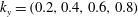 $k_{y}=(0.2,0.4,0.6,0.8)$
and
$k_{y}=(0.2,0.4,0.6,0.8)$
and
 $k_{x}=j2\unicode[STIX]{x03C0}n_{\text{pol}}|{\hat{s}}|k_{y}$
for integer
$k_{x}=j2\unicode[STIX]{x03C0}n_{\text{pol}}|{\hat{s}}|k_{y}$
for integer
 $j=(0,\pm 1,\ldots ,\pm 8)$
, and is shown in figure 2. As expected for pure
$j=(0,\pm 1,\ldots ,\pm 8)$
, and is shown in figure 2. As expected for pure
 $\unicode[STIX]{x1D735}n$
-driven TEM, almost all of the unstable modes are propagating in the electron-diamagnetic direction, corresponding to negative value for real frequency using Gene conventions. Examples of different mode types are given by the letter labels and the corresponding mode structures are shown in figure 3. There is a clustering of modes around zero real frequency, labelled by ‘C’, which have extended structure along field lines, consistent with the previous findings of Nadeem et al. (Reference Nadeem, Rafiq and Persson2001). The modes with definite non-zero frequencies, ‘A’ and ‘B’ tend to be much more strongly localized in helical drift wells. These modes do not need to balloon around
$\unicode[STIX]{x1D735}n$
-driven TEM, almost all of the unstable modes are propagating in the electron-diamagnetic direction, corresponding to negative value for real frequency using Gene conventions. Examples of different mode types are given by the letter labels and the corresponding mode structures are shown in figure 3. There is a clustering of modes around zero real frequency, labelled by ‘C’, which have extended structure along field lines, consistent with the previous findings of Nadeem et al. (Reference Nadeem, Rafiq and Persson2001). The modes with definite non-zero frequencies, ‘A’ and ‘B’ tend to be much more strongly localized in helical drift wells. These modes do not need to balloon around
 $\unicode[STIX]{x1D703}=0$
, and they display significant finite-
$\unicode[STIX]{x1D703}=0$
, and they display significant finite-
 $k_{x}$
amplitudes as well as tearing parity in electrostatic potential
$k_{x}$
amplitudes as well as tearing parity in electrostatic potential
 $\unicode[STIX]{x1D6F7}$
, consistent with previous observations of TEMs in HSX (Faber et al.
Reference Faber, Pueschel, Proll, Xanthopoulos, Terry, Hegna, Weir, Likin and Talmadge2015). For most modes in the spectrum, increasing the number of poloidal turns leads to a decrease in the growth rates, and is shown in figure 4 for
$\unicode[STIX]{x1D6F7}$
, consistent with previous observations of TEMs in HSX (Faber et al.
Reference Faber, Pueschel, Proll, Xanthopoulos, Terry, Hegna, Weir, Likin and Talmadge2015). For most modes in the spectrum, increasing the number of poloidal turns leads to a decrease in the growth rates, and is shown in figure 4 for
 $k_{y}=0.2$
for one and four poloidal turns. This behaviour is connected to the fact that by using more poloidal turns to construct the flux tube, more correct drive and damping physics is included, leading to a more accurate growth rate and frequency calculation for extended modes.
$k_{y}=0.2$
for one and four poloidal turns. This behaviour is connected to the fact that by using more poloidal turns to construct the flux tube, more correct drive and damping physics is included, leading to a more accurate growth rate and frequency calculation for extended modes.
Eigenspectrum for the strongly driven
 $\unicode[STIX]{x1D735}n$
TEM in HSX. The horizontal axis is the growth rate
$\unicode[STIX]{x1D735}n$
TEM in HSX. The horizontal axis is the growth rate
 $\unicode[STIX]{x1D6FE}$
and the vertical axis is the real frequency
$\unicode[STIX]{x1D6FE}$
and the vertical axis is the real frequency
 $\unicode[STIX]{x1D714}$
. Different
$\unicode[STIX]{x1D714}$
. Different
 $k_{y}$
are indicated different symbols and colours. Examples of different types of modes are given by the labels ‘A’ (
$k_{y}$
are indicated different symbols and colours. Examples of different types of modes are given by the labels ‘A’ (
 $k_{y}=0.8$
), ‘B’ (
$k_{y}=0.8$
), ‘B’ (
 $k_{y}=0.4$
), ‘C’ (
$k_{y}=0.4$
), ‘C’ (
 $k_{y}=0.8$
) and ‘D’ (
$k_{y}=0.8$
) and ‘D’ (
 $k_{y}=0.4$
), and the mode structure is shown in figure 3.
$k_{y}=0.4$
), and the mode structure is shown in figure 3.
Electrostatic potential eigenmode structures for the TEM branches labelled ‘A’ (upper left), ‘B’ (upper right), ‘C’ (lower left) and ‘D’ (lower right) from figure 2. The modes show conventional ballooning behaviour (A), finite
 $k_{x}$
dependence (B), extended structure along the field line (C) and two-scale structure with an extended envelope along the field line (D).
$k_{x}$
dependence (B), extended structure along the field line (C) and two-scale structure with an extended envelope along the field line (D).

A peculiar branch of eigenmodes, labelled ‘D’ in figure 2 is characterized by marginal stability modes, with a real frequency proportional to
 $k_{y}$
in the ion diamagnetic direction. The structure of the electrostatic potential along the field line for the eigenmodes in HSX, shown in figure 3 D, displays an extended, two-scale structure, with the outer scale varying on scales much longer than local helical drift wells. While these modes appear connected to small-global-magnetic-shear values, the exact mechanism responsible for setting the outer-scale envelope has not yet been determined. In the reverse-shear tokamak scenario studied in Candy et al. (Reference Candy, Waltz and Rosenbluth2004), the small, but non-zero global magnetic shear set the envelope scale. In 3-D configurations, variations in the local shear can determine mode localization through Mathieu resonances (Bhattacharjee et al.
Reference Bhattacharjee, Sedlak, Similon, Rosenbluth and Ross1983) or through a method similar to Anderson localization, where incommensurate helical periods in the magnetic equilibrium cause localization (Cuthbert & Dewar Reference Cuthbert and Dewar2000; Hegna & Hudson Reference Hegna and Hudson2001). The mode branch displays eigenmode structures with higher-harmonic envelopes that are increasingly damped.
$k_{y}$
in the ion diamagnetic direction. The structure of the electrostatic potential along the field line for the eigenmodes in HSX, shown in figure 3 D, displays an extended, two-scale structure, with the outer scale varying on scales much longer than local helical drift wells. While these modes appear connected to small-global-magnetic-shear values, the exact mechanism responsible for setting the outer-scale envelope has not yet been determined. In the reverse-shear tokamak scenario studied in Candy et al. (Reference Candy, Waltz and Rosenbluth2004), the small, but non-zero global magnetic shear set the envelope scale. In 3-D configurations, variations in the local shear can determine mode localization through Mathieu resonances (Bhattacharjee et al.
Reference Bhattacharjee, Sedlak, Similon, Rosenbluth and Ross1983) or through a method similar to Anderson localization, where incommensurate helical periods in the magnetic equilibrium cause localization (Cuthbert & Dewar Reference Cuthbert and Dewar2000; Hegna & Hudson Reference Hegna and Hudson2001). The mode branch displays eigenmode structures with higher-harmonic envelopes that are increasingly damped.
TEM eigenspectrum at
 $k_{y}=0.2$
for different poloidal turn values. Modes from one poloidal turn are the solid red diamonds and from four poloidal turns are the hollow blue diamonds. Generally, the modes at four poloidal turns are more stable, and there are fewer unstable modes than for one poloidal turn. Importantly, the extended ion mode branch (mode ‘D’ in figure 3), transitions from unstable to stable at four poloidal turns.
$k_{y}=0.2$
for different poloidal turn values. Modes from one poloidal turn are the solid red diamonds and from four poloidal turns are the hollow blue diamonds. Generally, the modes at four poloidal turns are more stable, and there are fewer unstable modes than for one poloidal turn. Importantly, the extended ion mode branch (mode ‘D’ in figure 3), transitions from unstable to stable at four poloidal turns.

Like the other eigenmodes, the growth rate of the extended ion mode branch is sensitive to the number of poloidal turns used to resolve the geometry. Figure 4 shows the extended ion mode branch at
 $\unicode[STIX]{x1D714}\approx 0.8$
is sensitive to the number of poloidal turns and that the linear damping increases with number of poloidal turns. At one poloidal turn, this mode branch even shows slight instability at
$\unicode[STIX]{x1D714}\approx 0.8$
is sensitive to the number of poloidal turns and that the linear damping increases with number of poloidal turns. At one poloidal turn, this mode branch even shows slight instability at
 $k_{y}=0.2$
. This sensitivity is observed despite the parallel correlation lengths of these modes being significantly larger than a few poloidal turns. In the analysis presented in Cuthbert & Dewar (Reference Cuthbert and Dewar2000) and Candy et al. (Reference Candy, Waltz and Rosenbluth2004), the eigenvalue is dependent on the solution to the inner-scale equation. More accurately resolving the inner-scale solution associated with the helical drift wells serves to stabilize the overall growth rate. Improperly resolving this extended scale mode has consequences for nonlinear simulation, as will be detailed in § 4.
$k_{y}=0.2$
. This sensitivity is observed despite the parallel correlation lengths of these modes being significantly larger than a few poloidal turns. In the analysis presented in Cuthbert & Dewar (Reference Cuthbert and Dewar2000) and Candy et al. (Reference Candy, Waltz and Rosenbluth2004), the eigenvalue is dependent on the solution to the inner-scale equation. More accurately resolving the inner-scale solution associated with the helical drift wells serves to stabilize the overall growth rate. Improperly resolving this extended scale mode has consequences for nonlinear simulation, as will be detailed in § 4.
3.2 Ion temperature gradient modes
Calculations of ITG eigenmodes in the HSX configuration have been performed, focusing on a pure collisionless ITG drive with kinetic electrons and the following parameters:
 $a/L_{T\text{i}}=3$
,
$a/L_{T\text{i}}=3$
,
 $a/L_{T\text{e}}=0$
,
$a/L_{T\text{e}}=0$
,
 $a/L_{n}=0$
,
$a/L_{n}=0$
,
 $T_{\text{i}}/T_{\text{e}}=1$
,
$T_{\text{i}}/T_{\text{e}}=1$
,
 $\unicode[STIX]{x1D6FD}=5\times 10^{-4}$
. Because the impact of eigenmodes with large parallel correlation lengths is more prevalent at low
$\unicode[STIX]{x1D6FD}=5\times 10^{-4}$
. Because the impact of eigenmodes with large parallel correlation lengths is more prevalent at low
 $k_{y}$
, the eigenspectrum is shown for
$k_{y}$
, the eigenspectrum is shown for
 $k_{y}<1$
in figure 5. As was observed with the TEM calculations, there are many unstable eigenmodes for every
$k_{y}<1$
in figure 5. As was observed with the TEM calculations, there are many unstable eigenmodes for every
 $k_{y}$
. A similar mix of mode structures is observed, including strongly ballooning modes,
$k_{y}$
. A similar mix of mode structures is observed, including strongly ballooning modes,
 $k_{x}\neq 0$
modes, and extended modes along the field line. Also observed are two-scale, ion-direction-propagating modes with extended-envelope structure, labelled by ‘A’, ‘B’ and ‘C’ in figure 5. The corresponding mode structures are shown in figure 6. While these modes have similar envelope behaviour as in the TEM case, a distinguishing characteristic of the ITG case is that these modes are much more unstable and do not become stable with increasing poloidal turns. Additionally, instability of the extended ion modes is observed at high
$k_{x}\neq 0$
modes, and extended modes along the field line. Also observed are two-scale, ion-direction-propagating modes with extended-envelope structure, labelled by ‘A’, ‘B’ and ‘C’ in figure 5. The corresponding mode structures are shown in figure 6. While these modes have similar envelope behaviour as in the TEM case, a distinguishing characteristic of the ITG case is that these modes are much more unstable and do not become stable with increasing poloidal turns. Additionally, instability of the extended ion modes is observed at high
 $k_{y}$
for the ITG case, as shown for
$k_{y}$
for the ITG case, as shown for
 $k_{y}=0.9$
in figure 5, while only marginal instability is observed at low
$k_{y}=0.9$
in figure 5, while only marginal instability is observed at low
 $k_{y}$
in figure 2 for the TEM case.
$k_{y}$
in figure 2 for the TEM case.
ITG eigenmode spectrum for different
 $k_{y}$
values, denoted by different symbols and colours. The modes at
$k_{y}$
values, denoted by different symbols and colours. The modes at
 $k_{y}=0.9$
labelled ‘A’, ‘B’ and ‘C’ are modes with two-scale behaviour, and the mode structures are shown in figure 6.
$k_{y}=0.9$
labelled ‘A’, ‘B’ and ‘C’ are modes with two-scale behaviour, and the mode structures are shown in figure 6.

Electrostatic potential for eigenmodes ‘A’ (top), ‘B’ (middle) and ‘C’ (bottom) from figure 5. The real part is the solid line and the imaginary part is the dotted black line. Similar to the mode ‘D’ in figure 3, the ITG eigenmodes display two-scale structure, with an outer-scale envelope and inner-scale structure set by the helical magnetic structure.

Despite these differences, given that these two-scale, extended-envelope ion modes are observed in both TEM and ITG calculations, the existence of these modes is connected to the low-magnetic-shear nature of devices such as HSX rather than a particular instability drive. An important observation is that these modes are not observed in the unstable eigenspectrum when an adiabatic electron approximation is used. This is shown in figure 7, where the eigenvalue spectrum is computed for both the adiabatic and kinetic electron treatment for a particular
 $k_{y}$
. Thus to fully resolve the drift-wave dynamics in a low-shear stellarator like HSX, it is important that kinetic electrons are used, so that crucial physics is not overlooked.
$k_{y}$
. Thus to fully resolve the drift-wave dynamics in a low-shear stellarator like HSX, it is important that kinetic electrons are used, so that crucial physics is not overlooked.
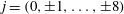
3.3 Zero-magnetic-shear approximation
The HSX shear value,
 ${\hat{s}}=-0.046$
, represents only a small deviation from
${\hat{s}}=-0.046$
, represents only a small deviation from
 ${\hat{s}}=0$
. Equation (2.2) shows that order-unity variations in
${\hat{s}}=0$
. Equation (2.2) shows that order-unity variations in
 $\unicode[STIX]{x1D735}\unicode[STIX]{x1D703}$
and
$\unicode[STIX]{x1D735}\unicode[STIX]{x1D703}$
and
 $\unicode[STIX]{x1D735}\unicode[STIX]{x1D701}$
terms will dominate over the secular
$\unicode[STIX]{x1D735}\unicode[STIX]{x1D701}$
terms will dominate over the secular
 $\unicode[STIX]{x1D735}\unicode[STIX]{x1D713}$
term, provided
$\unicode[STIX]{x1D735}\unicode[STIX]{x1D713}$
term, provided
 $\unicode[STIX]{x1D703}-\unicode[STIX]{x1D703}_{k}$
is small. A reasonable approximation for ballooning modes is then to neglect the global magnetic shear, which will be referred to as the zero-shear technique. In the zero-shear approach, linear modes no longer couple through magnetic shear, as the boundary condition is strictly periodic. A substantial benefit of this approach to low-magnetic-shear configurations is that the radial box size of the simulation is no longer determined by (A 7), which states
$\unicode[STIX]{x1D703}-\unicode[STIX]{x1D703}_{k}$
is small. A reasonable approximation for ballooning modes is then to neglect the global magnetic shear, which will be referred to as the zero-shear technique. In the zero-shear approach, linear modes no longer couple through magnetic shear, as the boundary condition is strictly periodic. A substantial benefit of this approach to low-magnetic-shear configurations is that the radial box size of the simulation is no longer determined by (A 7), which states
 $L_{x}\propto ({\hat{s}}k_{y}^{\text{min}})^{-1}$
. For HSX, using
$L_{x}\propto ({\hat{s}}k_{y}^{\text{min}})^{-1}$
. For HSX, using
 $k_{y}^{\text{min}}=0.1$
yields
$k_{y}^{\text{min}}=0.1$
yields
 $L_{x}\approx 220\unicode[STIX]{x1D70C}_{\text{s}}$
, a value comparable with macroscopic equilibrium scale lengths (Faber et al.
Reference Faber, Pueschel, Proll, Xanthopoulos, Terry, Hegna, Weir, Likin and Talmadge2015). Despite such large simulation domains, this is not physically problematic provided the turbulent correlation lengths are both smaller than experimental correlation lengths and the background length scales, such as
$L_{x}\approx 220\unicode[STIX]{x1D70C}_{\text{s}}$
, a value comparable with macroscopic equilibrium scale lengths (Faber et al.
Reference Faber, Pueschel, Proll, Xanthopoulos, Terry, Hegna, Weir, Likin and Talmadge2015). Despite such large simulation domains, this is not physically problematic provided the turbulent correlation lengths are both smaller than experimental correlation lengths and the background length scales, such as
 $L_{n,T}$
. A large radial box can be thought of as equivalent to multiple ‘independent’ simulation domains and turbulent statistics can be accumulated quickly. The numerical resolution, however, must also be scaled appropriately, making such simulations expensive to carry out. With zero magnetic shear, one may choose a more reasonable radial domain size and resolution, potentially reducing computational costs.
$L_{n,T}$
. A large radial box can be thought of as equivalent to multiple ‘independent’ simulation domains and turbulent statistics can be accumulated quickly. The numerical resolution, however, must also be scaled appropriately, making such simulations expensive to carry out. With zero magnetic shear, one may choose a more reasonable radial domain size and resolution, potentially reducing computational costs.
Comparison of the ITG eigenmode spectrum at
 $k_{y}=0.9$
for kinetic electrons (red) and adiabatic electrons (blue). Adding kinetic electron effects primarily the real frequency and reduces the number of unstable modes. However the extended ion modes that are unstable for kinetic electrons are absent from adiabatic electron calculations.
$k_{y}=0.9$
for kinetic electrons (red) and adiabatic electrons (blue). Adding kinetic electron effects primarily the real frequency and reduces the number of unstable modes. However the extended ion modes that are unstable for kinetic electrons are absent from adiabatic electron calculations.

With
 ${\hat{s}}=0$
, an extended parallel computational domain cannot be constructed by adding radial modes, as demonstrated in § 2. Zero-shear calculations then require that the parallel computation domain extend sufficiently far along the field line to better accommodate physical parallel correlation lengths. The strictly periodic boundary condition makes it easier to enhance growth rates through self-correlation if an eigenmode is not sufficiently decayed at the ends of the simulations domain. This is not only an issue for linear eigenmode calculations. A nonlinear simulation can be dominated by artificial linear self-correlation if growth rates are large enough compared to nonlinear decorrelation rates, which is demonstrated in § 4.
${\hat{s}}=0$
, an extended parallel computational domain cannot be constructed by adding radial modes, as demonstrated in § 2. Zero-shear calculations then require that the parallel computation domain extend sufficiently far along the field line to better accommodate physical parallel correlation lengths. The strictly periodic boundary condition makes it easier to enhance growth rates through self-correlation if an eigenmode is not sufficiently decayed at the ends of the simulations domain. This is not only an issue for linear eigenmode calculations. A nonlinear simulation can be dominated by artificial linear self-correlation if growth rates are large enough compared to nonlinear decorrelation rates, which is demonstrated in § 4.
Figure 8 shows the application of the zero-shear computational technique to HSX for dominant TEM eigenmode calculations where only one poloidal turn was used for the geometry. In a finite-shear simulation, due to linear
 $k_{x}$
coupling, the fastest growing connected
$k_{x}$
coupling, the fastest growing connected
 $k_{x}$
mode determines the overall mode growth rate. As linear modes are not coupled in zero-shear simulations, one must independently scan over
$k_{x}$
mode determines the overall mode growth rate. As linear modes are not coupled in zero-shear simulations, one must independently scan over
 $k_{x}$
to capture finite
$k_{x}$
to capture finite
 $k_{x}$
effects. At higher
$k_{x}$
effects. At higher
 $k_{y}$
, the finite-shear and zero-shear calculations agree quite well for
$k_{y}$
, the finite-shear and zero-shear calculations agree quite well for
 $k_{x}=0$
, where the most unstable modes strongly balloon at the outboard midplane and are sufficiently localized within one poloidal turn. For intermediate values
$k_{x}=0$
, where the most unstable modes strongly balloon at the outboard midplane and are sufficiently localized within one poloidal turn. For intermediate values
 $0.3\leqslant k_{y}\leqslant 0.7$
, strong growth at finite
$0.3\leqslant k_{y}\leqslant 0.7$
, strong growth at finite
 $k_{x}$
is observed and scanning
$k_{x}$
is observed and scanning
 $k_{x}$
for the zero-shear modes reproduces the finite-shear values. However, for
$k_{x}$
for the zero-shear modes reproduces the finite-shear values. However, for
 $k_{y}<0.2$
, clear divergences are observed between the zero-shear and finite-shear calculations. The zero-shear growth rates exhibit significantly larger growth rates than the finite-shear counterparts and can be identified as the zero-shear counterpart to the extended envelope ion modes in the finite-shear case. As is shown in figure 9, for geometry using one poloidal turn, this zero-shear mode branch (red diamonds) tracks the finite-shear (black diamonds) growth rates and frequencies relatively well for higher
$k_{y}<0.2$
, clear divergences are observed between the zero-shear and finite-shear calculations. The zero-shear growth rates exhibit significantly larger growth rates than the finite-shear counterparts and can be identified as the zero-shear counterpart to the extended envelope ion modes in the finite-shear case. As is shown in figure 9, for geometry using one poloidal turn, this zero-shear mode branch (red diamonds) tracks the finite-shear (black diamonds) growth rates and frequencies relatively well for higher
 $k_{y}$
values. Around
$k_{y}$
values. Around
 $k_{y}=0.3$
, the zero-shear growth rates diverge and become significantly more unstable. This is problematic for nonlinear simulations that require
$k_{y}=0.3$
, the zero-shear growth rates diverge and become significantly more unstable. This is problematic for nonlinear simulations that require
 $k_{y}^{\text{min}}\leqslant 0.1$
, and will be discussed in § 4.
$k_{y}^{\text{min}}\leqslant 0.1$
, and will be discussed in § 4.
Linear growth rate spectrum of TEMs for one poloidal turn for the finite-shear approach (red) and the zero-shear approach (black and blue). The blue points are from calculations where the
 $k_{x}$
value was varied to find the maximum growth rate, while the black points are the
$k_{x}$
value was varied to find the maximum growth rate, while the black points are the
 $k_{x}=0$
streamer instability. The non-zero
$k_{x}=0$
streamer instability. The non-zero
 $k_{x}$
effects are required to reproduce the finite-shear spectrum for
$k_{x}$
effects are required to reproduce the finite-shear spectrum for
 $0.3\leqslant k_{y}\leqslant 0.7$
.
$0.3\leqslant k_{y}\leqslant 0.7$
.

Eigenspectrum of the artificially enhanced mode (red diamonds) of figure 8 for a range of wavenumbers
 $k_{y}$
. Select
$k_{y}$
. Select
 $k_{y}$
modes are identified by the outlined symbols and compared with the finite-shear counterpart for one poloidal turn (black diamonds). All finite-shear eigenvalues are clustered near marginal stability, whereas zero-shear modes are artificially enhanced at one poloidal turn.
$k_{y}$
modes are identified by the outlined symbols and compared with the finite-shear counterpart for one poloidal turn (black diamonds). All finite-shear eigenvalues are clustered near marginal stability, whereas zero-shear modes are artificially enhanced at one poloidal turn.

Linear mode differences between the finite and zero-shear techniques become small when multiple poloidal turns are utilized, and in particular, growth rate differences at wavenumbers
 $k_{y}\leqslant 0.1$
are significantly reduced. The periodic parallel boundary conditions coupled with geometry from one poloidal turn does not allow modes to sufficiently decay and the growth rate is artificially enhanced. This indicates that for the low-
$k_{y}\leqslant 0.1$
are significantly reduced. The periodic parallel boundary conditions coupled with geometry from one poloidal turn does not allow modes to sufficiently decay and the growth rate is artificially enhanced. This indicates that for the low-
 $k_{y}$
modes, the parallel correlation lengths for HSX are longer than one poloidal turn and that the enhanced growth rates for the zero-shear calculations were due to self-correlating fluctuations. For the half-toroidal flux surface in HSX, linear TEMs show convergence at 4 poloidal turns.
$k_{y}$
modes, the parallel correlation lengths for HSX are longer than one poloidal turn and that the enhanced growth rates for the zero-shear calculations were due to self-correlating fluctuations. For the half-toroidal flux surface in HSX, linear TEMs show convergence at 4 poloidal turns.
As noted previously, for stellarator purposes, it is not sufficient to just examine convergence of the most unstable mode, as subdominant modes can play an important role in the turbulent dynamics. Figure 10 shows a comparison of the eigenmode spectrum between the finite and zero-shear techniques for a TEM case in HSX, using four poloidal turns at
 $k_{y}=0.7$
. The zero-shear eigenmodes are computed by scanning
$k_{y}=0.7$
. The zero-shear eigenmodes are computed by scanning
 $k_{x}$
values that would be coupled via the parallel boundary condition in the finite-shear calculation. Figure 10 shows that both the zero-shear and finite-shear growth rates across the spectrum are replicated. It is not necessary to match exactly every single subdominant mode between the two approaches. Pueschel et al. (Reference Pueschel, Faber, Citrin, Hegna, Terry and Hatch2016) demonstrated the impact of the subdominant modes in HSX is to generate broadband turbulence, lessening the impact of any particular eigenmode. More importantly, the clustering of eigenmodes in the spectrum is very well reproduced between the calculation techniques in figure 10, which leads to consistent turbulence energy drive and dissipation. This gives confidence that the zero-shear technique is accurately calculating the eigenmode spectrum when the parallel correlation length is sufficiently resolved.
$k_{x}$
values that would be coupled via the parallel boundary condition in the finite-shear calculation. Figure 10 shows that both the zero-shear and finite-shear growth rates across the spectrum are replicated. It is not necessary to match exactly every single subdominant mode between the two approaches. Pueschel et al. (Reference Pueschel, Faber, Citrin, Hegna, Terry and Hatch2016) demonstrated the impact of the subdominant modes in HSX is to generate broadband turbulence, lessening the impact of any particular eigenmode. More importantly, the clustering of eigenmodes in the spectrum is very well reproduced between the calculation techniques in figure 10, which leads to consistent turbulence energy drive and dissipation. This gives confidence that the zero-shear technique is accurately calculating the eigenmode spectrum when the parallel correlation length is sufficiently resolved.
Comparison of the finite-shear (hollow red diamonds) and zero-shear (solid black diamonds) eigenspectrum at
 $k_{y}=0.7$
for the
$k_{y}=0.7$
for the
 $\unicode[STIX]{x1D735}n$
-driven TEM. Sufficient agreement is observed between the two computational approaches when multiple poloidal turns are used. In particular, the zero-shear technique recovers the appropriate clustering of eigenmodes, including the marginally stable ion mode branch (branch ‘D’ of figure 2).
$\unicode[STIX]{x1D735}n$
-driven TEM. Sufficient agreement is observed between the two computational approaches when multiple poloidal turns are used. In particular, the zero-shear technique recovers the appropriate clustering of eigenmodes, including the marginally stable ion mode branch (branch ‘D’ of figure 2).
4 Nonlinear effects
The impact of multiple poloidal turns and the necessity to accurately resolve the subdominant spectrum can be seen in nonlinear simulations. TEM turbulence simulations are performed using the plasma parameters of § 3.1 with
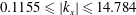 $0.1155\leqslant |k_{x}|\leqslant 14.784$
,
$0.1155\leqslant |k_{x}|\leqslant 14.784$
,
 $k_{y}^{\text{max}}=3.1$
and two separate
$k_{y}^{\text{max}}=3.1$
and two separate
 $k_{y}^{\text{min}}$
values,
$k_{y}^{\text{min}}$
values,
 $k_{y}^{\text{min}}=0.05,0.1$
. Figure 11 shows values of electron electrostatic heat flux from
$k_{y}^{\text{min}}=0.05,0.1$
. Figure 11 shows values of electron electrostatic heat flux from
 $\unicode[STIX]{x1D735}n$
-driven TEM turbulence simulations of HSX as a function of number of poloidal turns used to construct the flux-tube geometry. The heat flux shows numerical convergence only at four poloidal turns. Furthermore, agreement is seen between the finite-shear and zero-shear flux-tube approaches, but again only when multiple poloidal turns are used. For the high-density-gradient case here, with
$\unicode[STIX]{x1D735}n$
-driven TEM turbulence simulations of HSX as a function of number of poloidal turns used to construct the flux-tube geometry. The heat flux shows numerical convergence only at four poloidal turns. Furthermore, agreement is seen between the finite-shear and zero-shear flux-tube approaches, but again only when multiple poloidal turns are used. For the high-density-gradient case here, with
 $a/L_{n}=4$
, it is seen that with only one poloidal turn, even the finite-shear flux tubes with different
$a/L_{n}=4$
, it is seen that with only one poloidal turn, even the finite-shear flux tubes with different
 $k_{y}^{\text{min}}$
values have different transport levels, and only after four poloidal turns do the flux values agree. This suggests it is necessary to check for convergence in the number of poloidal turns used to construct the geometry when performing nonlinear simulations.
$k_{y}^{\text{min}}$
values have different transport levels, and only after four poloidal turns do the flux values agree. This suggests it is necessary to check for convergence in the number of poloidal turns used to construct the geometry when performing nonlinear simulations.
Nonlinear TEM heat fluxes for HSX as function of poloidal turns. In red and blue are finite-shear simulations with
 $k_{y}^{\text{min}}=0.1$
and 0.05 respectively, while zero-shear simulations are shown in black. Simulations agree for
$k_{y}^{\text{min}}=0.1$
and 0.05 respectively, while zero-shear simulations are shown in black. Simulations agree for
 $n_{\text{pol}}\geqslant 4$
.
$n_{\text{pol}}\geqslant 4$
.
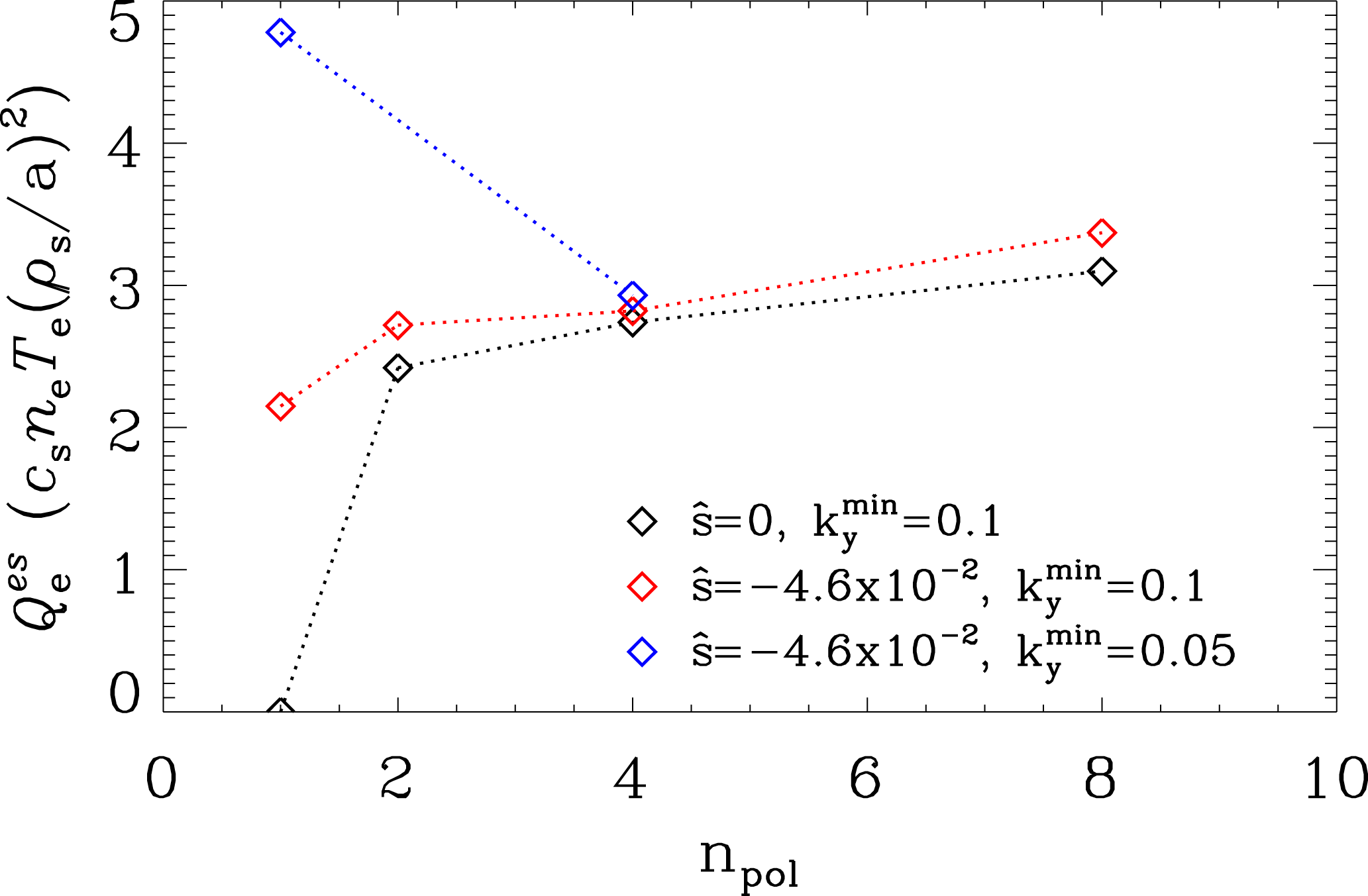
A striking observation from
 $\unicode[STIX]{x1D735}n$
-driven TEM simulations in HSX (Faber et al.
Reference Faber, Pueschel, Proll, Xanthopoulos, Terry, Hegna, Weir, Likin and Talmadge2015) is a peak in the electrostatic heat flux spectrum at
$\unicode[STIX]{x1D735}n$
-driven TEM simulations in HSX (Faber et al.
Reference Faber, Pueschel, Proll, Xanthopoulos, Terry, Hegna, Weir, Likin and Talmadge2015) is a peak in the electrostatic heat flux spectrum at
 $k_{y}^{\text{min}}\approx 0.1$
. This feature becomes more prominent as
$k_{y}^{\text{min}}\approx 0.1$
. This feature becomes more prominent as
 $a/L_{n}$
increases. The flux spectrum for the nonlinear TEM simulations of figure 11 is shown in figure 12. At only one poloidal turn, the magenta and teal curves, the flux peaks at the lowest non-zero
$a/L_{n}$
increases. The flux spectrum for the nonlinear TEM simulations of figure 11 is shown in figure 12. At only one poloidal turn, the magenta and teal curves, the flux peaks at the lowest non-zero
 $k_{y}$
and increases significantly as
$k_{y}$
and increases significantly as
 $k_{y}^{\text{min}}$
is decreased. However, when 4 poloidal turns are used, the flux continues to peak at
$k_{y}^{\text{min}}$
is decreased. However, when 4 poloidal turns are used, the flux continues to peak at
 $k_{y}=0.1$
, and is substantially smaller at
$k_{y}=0.1$
, and is substantially smaller at
 $k_{y}=0.05$
for the
$k_{y}=0.05$
for the
 $k_{y}^{\text{min}}=0.05$
simulation. This again indicates that only with four poloidal turns are the low-
$k_{y}^{\text{min}}=0.05$
simulation. This again indicates that only with four poloidal turns are the low-
 $k_{y}$
modes sufficiently resolved in the parallel direction such that accurate turbulence simulations are achieved.
$k_{y}$
modes sufficiently resolved in the parallel direction such that accurate turbulence simulations are achieved.
Flux spectrum from nonlinear TEM simulations for HSX. The different curves represent different combinations of poloidal turns used for the geometry and
 $k_{y}^{\text{min}}$
values. All curves, except for the black curve, were simulations with non-zero shear. The blue and teal dashed curves have been scaled by a factor of two due to having twice the
$k_{y}^{\text{min}}$
values. All curves, except for the black curve, were simulations with non-zero shear. The blue and teal dashed curves have been scaled by a factor of two due to having twice the
 $k_{y}$
resolution as the solid curves.
$k_{y}$
resolution as the solid curves.
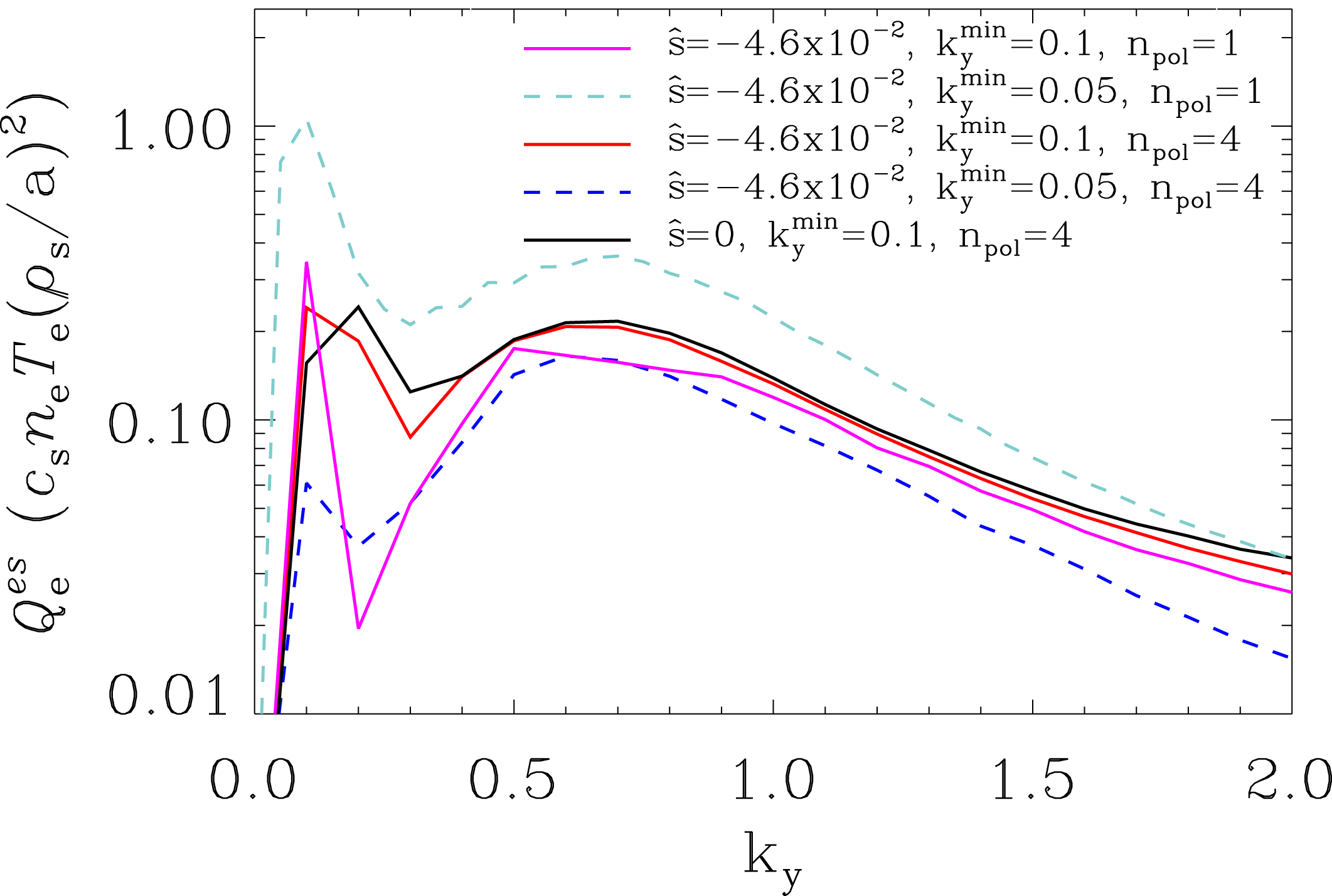
Insight into the physics driving transport at
 $k_{y}\approx 0.1$
and why simulations with only one poloidal turn are not converged can be obtained from nonlinear energy transfer considerations. For example, the equation for entropy transfer between modes at wavenumbers
$k_{y}\approx 0.1$
and why simulations with only one poloidal turn are not converged can be obtained from nonlinear energy transfer considerations. For example, the equation for entropy transfer between modes at wavenumbers
 $k$
and
$k$
and
 $k^{\prime }$
can be written as (Bañón Navarro et al.
Reference Bañón Navarro, Morel, Albrecht-Marc, Carati, Merz, Gorler and Jenko2011):
$k^{\prime }$
can be written as (Bañón Navarro et al.
Reference Bañón Navarro, Morel, Albrecht-Marc, Carati, Merz, Gorler and Jenko2011):
 $$\begin{eqnarray}{\mathcal{T}}_{f}^{k,k^{\prime }}=\int \text{d}z\,\text{d}v_{\Vert }\,\text{d}\unicode[STIX]{x1D707}\unicode[STIX]{x03C0}B_{0}n_{0\text{i}}\left[\frac{T_{0\text{i}}}{F_{0\text{i}}}f_{k}^{\ast }((k-k^{\prime })\bar{\unicode[STIX]{x1D719}}_{1(k-k^{\prime })}k_{y}^{\prime }\,f_{k^{\prime }}-(k-k^{\prime })\bar{\unicode[STIX]{x1D719}}_{1(k-k^{\prime })}k_{x}^{\prime }\,f_{k}^{\prime })\right],\end{eqnarray}$$
where the perturbed distribution function at wavenumber
 $k$
,
$k$
,
 $f_{k}$
, is a function the parallel coordinate
$f_{k}$
, is a function the parallel coordinate
 $z$
and velocity space coordinates
$z$
and velocity space coordinates
 $v_{\Vert }$
and
$v_{\Vert }$
and
 $\unicode[STIX]{x1D707}$
. The gyro-averaged fluctuating potential
$\unicode[STIX]{x1D707}$
. The gyro-averaged fluctuating potential
 $\bar{\unicode[STIX]{x1D719}}_{1k}$
is a function of
$\bar{\unicode[STIX]{x1D719}}_{1k}$
is a function of
 $z$
alone. While other nonlinear transfer terms can be identified in the energy budget equations, Bañón Navarro et al. (Reference Bañón Navarro, Morel, Albrecht-Marc, Carati, Merz, Gorler and Jenko2011) shows this term is the dominant transfer mechanism. The amount of entropy transferred by (4.1) can be increased by two methods. Large values of
$z$
alone. While other nonlinear transfer terms can be identified in the energy budget equations, Bañón Navarro et al. (Reference Bañón Navarro, Morel, Albrecht-Marc, Carati, Merz, Gorler and Jenko2011) shows this term is the dominant transfer mechanism. The amount of entropy transferred by (4.1) can be increased by two methods. Large values of
 ${\mathcal{T}}_{f}^{k,k^{\prime }}$
can be achieved when eigenmodes are correlated in both the parallel direction and in velocity space. Eigenmodes that are not well correlated, but still have some overlap, can have large
${\mathcal{T}}_{f}^{k,k^{\prime }}$
can be achieved when eigenmodes are correlated in both the parallel direction and in velocity space. Eigenmodes that are not well correlated, but still have some overlap, can have large
 ${\mathcal{T}}_{f}^{k,k^{\prime }}$
if the amplitudes are large enough to compensate for the lack of mode correlation.
${\mathcal{T}}_{f}^{k,k^{\prime }}$
if the amplitudes are large enough to compensate for the lack of mode correlation.
These considerations make it clear why zonal flows, which are uniform in
 $z$
, can efficiently transfer energy. Zonal flows, however, are linearly stable and only driven to large amplitudes by nonlinear energy transfer and cannot input energy into the system. Similar to zonal flows, the marginally stable ion mode branch has extended structure along field lines and Maxwellian velocity space structure, enabling efficient transfer of energy between modes. As seen in § § 3.1 and 3.2, however, the ion modes can be linearly unstable when an insufficient number of poloidal turns are used for the computational domain. These modes, which are more unstable at low
$z$
, can efficiently transfer energy. Zonal flows, however, are linearly stable and only driven to large amplitudes by nonlinear energy transfer and cannot input energy into the system. Similar to zonal flows, the marginally stable ion mode branch has extended structure along field lines and Maxwellian velocity space structure, enabling efficient transfer of energy between modes. As seen in § § 3.1 and 3.2, however, the ion modes can be linearly unstable when an insufficient number of poloidal turns are used for the computational domain. These modes, which are more unstable at low
 $k_{y}$
, can then also provide an energy drive for turbulence. This can be problematic for nonlinear simulations, as simulations of ion scale turbulence generally require
$k_{y}$
, can then also provide an energy drive for turbulence. This can be problematic for nonlinear simulations, as simulations of ion scale turbulence generally require
 $k_{y}^{\text{min}}\lesssim 0.1$
, and an important factor for converged nonlinear simulations is the avoidance of significant energy drive at the domain scales. The contribution to the linear energy drive from the modes at
$k_{y}^{\text{min}}\lesssim 0.1$
, and an important factor for converged nonlinear simulations is the avoidance of significant energy drive at the domain scales. The contribution to the linear energy drive from the modes at
 $k_{y}=0.2$
can be seen in figure 13, where the non-conservative energy evolution terms, including terms proportional to the driving density gradient, are plotted as a function of
$k_{y}=0.2$
can be seen in figure 13, where the non-conservative energy evolution terms, including terms proportional to the driving density gradient, are plotted as a function of
 $(k_{x},k_{y})$
. In situations where a single instability dominates, such as in most high-shear situations, figure 13 would show only the conical yellow structure seen for
$(k_{x},k_{y})$
. In situations where a single instability dominates, such as in most high-shear situations, figure 13 would show only the conical yellow structure seen for
 $|k_{y}|\gtrsim 0.3$
. The presence of strong energy drive at
$|k_{y}|\gtrsim 0.3$
. The presence of strong energy drive at
 $|k_{y}|=0.2$
suggests a connection to the extended ion modes, possibly through nonlinear, finite-amplitude instability as described in Friedman et al. (Reference Friedman, Carter, Umansky, Schaffner and Joseph2013), Friedman & Carter (Reference Friedman and Carter2014), or a pseudospectral response (Hatch et al.
Reference Hatch, Jenko, Bañón Navarro, Bratanov, Terry and Pueschel2016a
). Techniques for directly analysing the energy dynamics of specific eigenmodes (Whelan et al.
Reference Whelan, Pueschel and Terry2018) will be employed on these data in future work.
$|k_{y}|=0.2$
suggests a connection to the extended ion modes, possibly through nonlinear, finite-amplitude instability as described in Friedman et al. (Reference Friedman, Carter, Umansky, Schaffner and Joseph2013), Friedman & Carter (Reference Friedman and Carter2014), or a pseudospectral response (Hatch et al.
Reference Hatch, Jenko, Bañón Navarro, Bratanov, Terry and Pueschel2016a
). Techniques for directly analysing the energy dynamics of specific eigenmodes (Whelan et al.
Reference Whelan, Pueschel and Terry2018) will be employed on these data in future work.
The impact of the stability of the extended ion modes on nonlinear convergence are not just limited to the direct linear energy drive. If these modes are linearly unstable, they can grow to significant amplitudes and enhance nonlinear entropy and energy transfer. Due to their extended structure along the field line and Maxwellian velocity space structure, they can provide efficient coupling between eigenmodes, similar in manner to a zonal flow, and by extension also efficiently couple directly to zonal flows. This can have significant consequences for nonlinear simulations. Erroneously large zonal flow amplitudes will enhance the ability of zonal flows to transfer energy nonlinearly to damped modes. This is the mechanism responsible for the near zero heat flux observed in the zero-shear simulations at one poloidal turn in figure 11. The linear growth rates at low
 $k_{y}$
for the zero-shear simulations are significantly enhanced compared to the finite-shear simulations, as was seen in figure 8. Visually, this impact can be seen by examining the contours of fluctuating potential and density from a zero-shear nonlinear simulation, as shown in figure 14. The contours indicate the simulation is dominated by a coherent interaction between the zonal flows and a linear mode that spans the box, which for
$k_{y}$
for the zero-shear simulations are significantly enhanced compared to the finite-shear simulations, as was seen in figure 8. Visually, this impact can be seen by examining the contours of fluctuating potential and density from a zero-shear nonlinear simulation, as shown in figure 14. The contours indicate the simulation is dominated by a coherent interaction between the zonal flows and a linear mode that spans the box, which for
 $k_{y}^{\text{min}}=0.1$
is the artificially enhanced branch in figure 8.
$k_{y}^{\text{min}}=0.1$
is the artificially enhanced branch in figure 8.
Spectrum of non-conservative energy terms in units of
 $n_{0\text{e}}T_{0\text{e}}c_{\text{s}}\unicode[STIX]{x1D70C}_{\text{s}}^{2}/a^{3}$
for the high-
$n_{0\text{e}}T_{0\text{e}}c_{\text{s}}\unicode[STIX]{x1D70C}_{\text{s}}^{2}/a^{3}$
for the high-
 $\unicode[STIX]{x1D735}n$
TEM simulation for HSX. A positive (red)
$\unicode[STIX]{x1D735}n$
TEM simulation for HSX. A positive (red)
 $\text{d}E/\text{d}t$
value at a
$\text{d}E/\text{d}t$
value at a
 $(k_{x},k_{y})$
indicates energy is being input into the system. The modes at
$(k_{x},k_{y})$
indicates energy is being input into the system. The modes at
 $k_{y}=0.2$
have the largest
$k_{y}=0.2$
have the largest
 $\text{d}E/\text{d}t$
values, coinciding with the heat flux peak at
$\text{d}E/\text{d}t$
values, coinciding with the heat flux peak at
 $k_{y}=0.2$
in figure 12.
$k_{y}=0.2$
in figure 12.
Instantaneous contours of fluctuating electrostatic potential
 $\unicode[STIX]{x1D6F7}$
((a), in units of
$\unicode[STIX]{x1D6F7}$
((a), in units of
 $\unicode[STIX]{x1D70C}_{\text{s}}T_{0\text{e}}/(ea)$
) and density
$\unicode[STIX]{x1D70C}_{\text{s}}T_{0\text{e}}/(ea)$
) and density
 $n$
((b), in units of
$n$
((b), in units of
 $n_{0\text{e}}\unicode[STIX]{x1D70C}_{\text{s}}/a$
) from a zero-shear simulation with one poloidal turn (black curve of figure 11). Both
$n_{0\text{e}}\unicode[STIX]{x1D70C}_{\text{s}}/a$
) from a zero-shear simulation with one poloidal turn (black curve of figure 11). Both
 $\unicode[STIX]{x1D6F7}$
and
$\unicode[STIX]{x1D6F7}$
and
 $n$
display dominant zonal components, and the density shows a clear coherent mode.
$n$
display dominant zonal components, and the density shows a clear coherent mode.
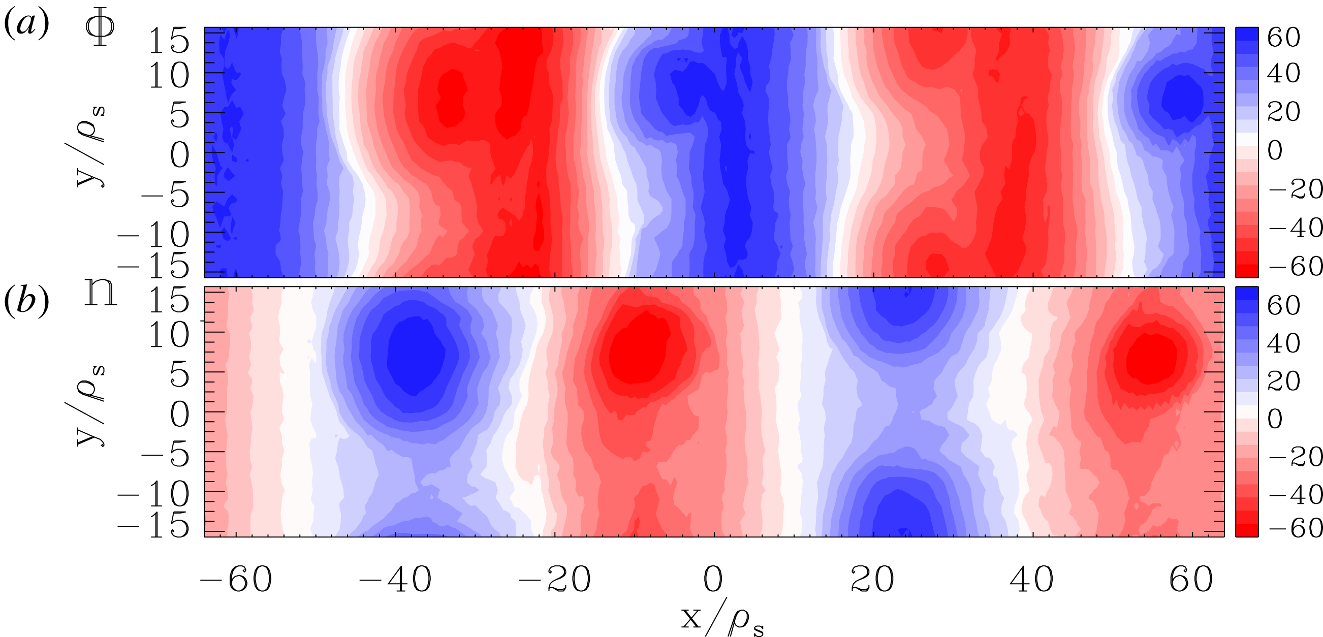
Signatures of the extended ion mode persist in the finite-shear simulations when multiple poloidal turns are used so that the extended ion modes transition from unstable to stable at low
 $k_{y}$
. To obtain the amplitude of an eigenmode in the nonlinear turbulent state, one can project the nonlinear distribution function onto the eigenmodes with the following relation:
$k_{y}$
. To obtain the amplitude of an eigenmode in the nonlinear turbulent state, one can project the nonlinear distribution function onto the eigenmodes with the following relation:
 $$\begin{eqnarray}p_{j}=\frac{\left|\displaystyle \int \text{d}\boldsymbol{x}\,\text{d}\boldsymbol{v}f_{j}^{\ast }f_{\text{NL}}\right|}{\left(\displaystyle \int \text{d}\boldsymbol{x}\,\text{d}\boldsymbol{v}|f_{j}|^{2}\int \text{d}\boldsymbol{x}\,\text{d}\boldsymbol{v}|f_{\text{NL}}|^{2}\right)^{1/2}}.\end{eqnarray}$$
Here,
 $p_{j}$
is the projection of the eigenmode
$p_{j}$
is the projection of the eigenmode
 $f_{j}$
and
$f_{j}$
and
 $f_{\text{NL}}$
is the nonlinear distribution function. The eigenmodes are not orthogonal, thus the projection
$f_{\text{NL}}$
is the nonlinear distribution function. The eigenmodes are not orthogonal, thus the projection
 $p_{j}$
is not uniquely associated with the amplitude for eigenmode
$p_{j}$
is not uniquely associated with the amplitude for eigenmode
 $f_{j}$
, but it can illuminate general trends in the underlying aspects of the turbulence. The projection onto the eigenmodes at
$f_{j}$
, but it can illuminate general trends in the underlying aspects of the turbulence. The projection onto the eigenmodes at
 $k_{y}=0.2$
of the turbulent distribution function for the high
$k_{y}=0.2$
of the turbulent distribution function for the high
 $\unicode[STIX]{x1D735}n$
-driven TEM case is shown in figure 15. This wavenumber corresponds to a region of low heat flux in figure 12.
$\unicode[STIX]{x1D735}n$
-driven TEM case is shown in figure 15. This wavenumber corresponds to a region of low heat flux in figure 12.
Projection of TEM turbulence onto eigenmodes at
 $k_{y}=0.2$
using geometry with four poloidal turns. The colour bar gives the projection value. The projection shows subdominant and stable modes have higher projection values than the most unstable modes. The inset figures show the potential mode structure of the high-projection modes, emphasizing that at
$k_{y}=0.2$
using geometry with four poloidal turns. The colour bar gives the projection value. The projection shows subdominant and stable modes have higher projection values than the most unstable modes. The inset figures show the potential mode structure of the high-projection modes, emphasizing that at
 $k_{y}=0.2$
, modes with extended structure along the field line play a large role in the nonlinear state.
$k_{y}=0.2$
, modes with extended structure along the field line play a large role in the nonlinear state.
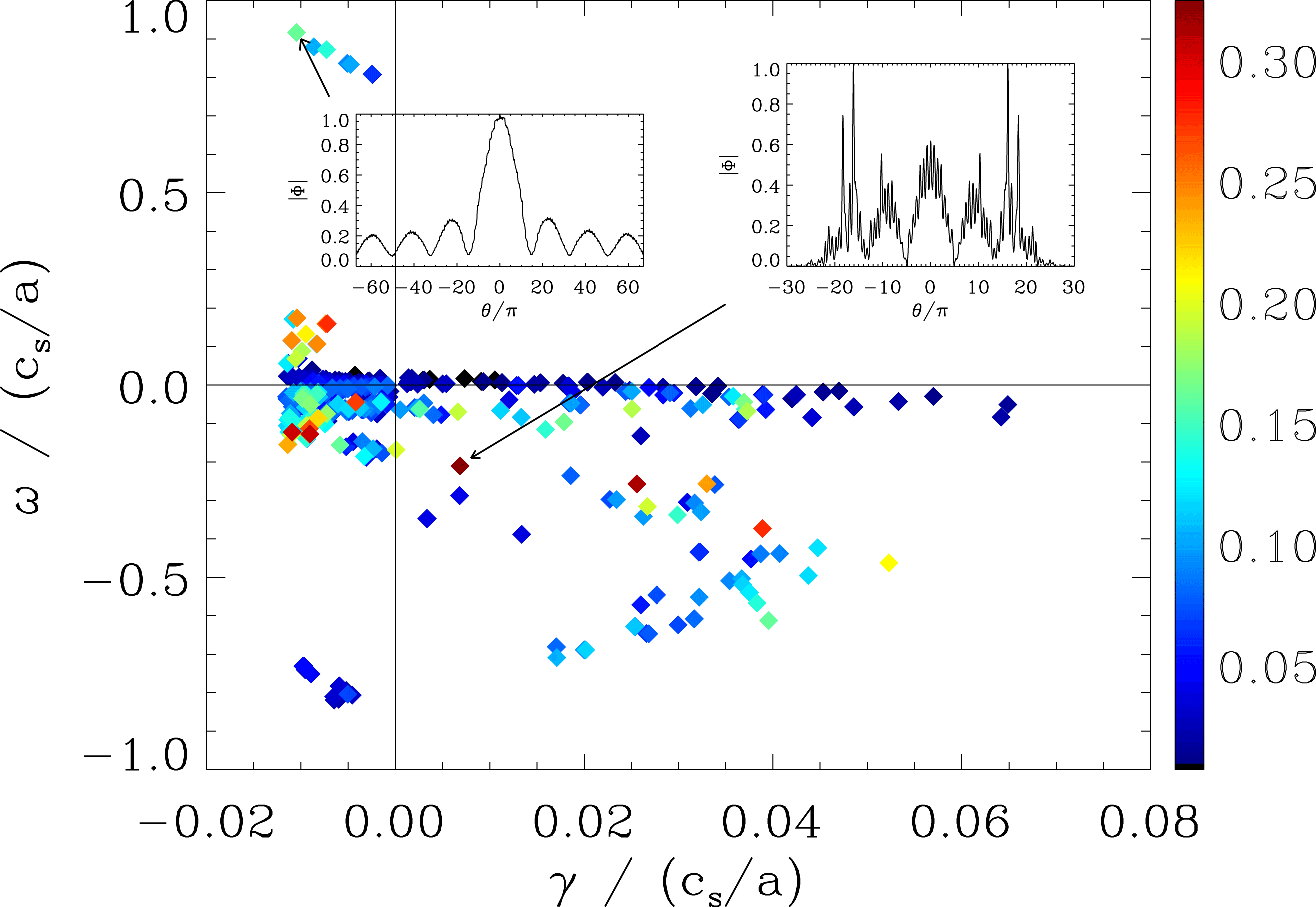
The figure demonstrates, consistent with previous observations, that subdominant modes have strong projection values while the most unstable modes have considerably smaller projections. The inset figures in figure 15 show that the modes with large projections have extended structure along the field line and that, somewhat counter-intuitively, the stable, extended-envelope ion modes have increasingly large projection values with increasing damping rate. At higher
 $k_{y}$
, where the majority of the flux is driven in figure 12, the projection selects the most unstable mode as having the largest imprint on the turbulence, as one would expect, even when subdominant modes are important (Pueschel et al.
Reference Pueschel, Faber, Citrin, Hegna, Terry and Hatch2016). This provides more evidence supporting the preceding discussion pertaining to (4.1) and figure 13 that the extended ion modes are acting as both a linear energy drive and have a dominant role nonlinear energy transfer.
$k_{y}$
, where the majority of the flux is driven in figure 12, the projection selects the most unstable mode as having the largest imprint on the turbulence, as one would expect, even when subdominant modes are important (Pueschel et al.
Reference Pueschel, Faber, Citrin, Hegna, Terry and Hatch2016). This provides more evidence supporting the preceding discussion pertaining to (4.1) and figure 13 that the extended ion modes are acting as both a linear energy drive and have a dominant role nonlinear energy transfer.
A plausible picture then emerges concerning both the lack of nonlinear convergence with one poloidal turn and the appearance of substantial heat flux seen in figure 12 at low
 $k_{y}$
. When the geometry is insufficiently resolved, the low-
$k_{y}$
. When the geometry is insufficiently resolved, the low-
 $k_{y}$
extended ion modes are linearly unstable due to self-correlation effects and can grow to high amplitudes in nonlinear simulations. Efficient nonlinear coupling can then pump both zonal flows and finite-
$k_{y}$
extended ion modes are linearly unstable due to self-correlation effects and can grow to high amplitudes in nonlinear simulations. Efficient nonlinear coupling can then pump both zonal flows and finite-
 $k_{y}$
modes that further enhance transport at low
$k_{y}$
modes that further enhance transport at low
 $k_{y}$
. When multiple poloidal turns are used to more accurately describe the geometry along the field line, the now linearly stable extended ion modes are still efficient channels for nonlinear energy transfer, but with much smaller amplitudes. Low-
$k_{y}$
. When multiple poloidal turns are used to more accurately describe the geometry along the field line, the now linearly stable extended ion modes are still efficient channels for nonlinear energy transfer, but with much smaller amplitudes. Low-
 $k_{y}$
modes can still be pumped to large enough amplitudes to drive the observed transport peak, but the relative lack of linear energy drive at low-
$k_{y}$
modes can still be pumped to large enough amplitudes to drive the observed transport peak, but the relative lack of linear energy drive at low-
 $k_{y}$
limits how much flux can be produced. It should be emphasized that this is an effect of subdominant and stable modes at low magnetic shear. If the turbulence was set by interactions between the most unstable mode and the nonlinearity, as is generally the case for higher-shear configurations where extended modes becomes more stable, the turbulence would be insensitive to the parallel resolution, as the most unstable modes are accurately resolved by geometries constructed using one poloidal turn. This indicates that for low-magnetic-shear stellarators, one must ensure the subdominant eigenspectrum is accurately simulated.
$k_{y}$
limits how much flux can be produced. It should be emphasized that this is an effect of subdominant and stable modes at low magnetic shear. If the turbulence was set by interactions between the most unstable mode and the nonlinearity, as is generally the case for higher-shear configurations where extended modes becomes more stable, the turbulence would be insensitive to the parallel resolution, as the most unstable modes are accurately resolved by geometries constructed using one poloidal turn. This indicates that for low-magnetic-shear stellarators, one must ensure the subdominant eigenspectrum is accurately simulated.
5 Conclusions
In this work, we have presented a detailed study of the influence of low global magnetic shear on flux-tube gyrokinetic simulations of the HSX configuration. In order to achieve converged nonlinear simulations, the flux tube needs to be constructed with geometry data from multiple poloidal turns. Using multiple poloidal turns more accurately resolves parallel mode structure and correlation crucial to accurately describing instability drive and damping physics. When only one poloidal turn is used, self-correlation occurs for modes that have parallel correlation lengths larger than one poloidal turn, artificially enhancing growth rates. These artificially enhanced modes can in turn dominate nonlinear simulations, as is observed for zero-magnetic-shear simulations, leading to loss of numerical convergence. Numerical convergence and agreement between finite-shear and zero-shear computational techniques is observed when multiple poloidal turns are used. For the HSX flux tubes studied here, at least four poloidal turns are required.
Properly resolved simulations reveal a wealth of complex behaviour for HSX in both linear eigenmode calculations and nonlinear simulations. Many different unstable eigenmodes are observed at each
 $k_{y}$
for both TEM and ITG calculations. Of particular interest is a branch of modes propagating in the ion-diagmagnetic direction that has two-scale structure, with an outer-scale envelope extending far along the field line and the inner scale is set by the local helical structure along the field line. These modes are marginally stable for TEM calculations, but are unstable, though still subdominant, for ITG calculations. In nonlinear TEM turbulence simulations for HSX, these extended ion modes play a prominent role in the nonlinear dynamics. Owing to their extended structure along field lines and Maxwellian velocity space structure, they provide efficient channels for nonlinear energy transfer, similar in manner to zonal flows. Furthermore, and unlike zonal flows since they have non-zero
$k_{y}$
for both TEM and ITG calculations. Of particular interest is a branch of modes propagating in the ion-diagmagnetic direction that has two-scale structure, with an outer-scale envelope extending far along the field line and the inner scale is set by the local helical structure along the field line. These modes are marginally stable for TEM calculations, but are unstable, though still subdominant, for ITG calculations. In nonlinear TEM turbulence simulations for HSX, these extended ion modes play a prominent role in the nonlinear dynamics. Owing to their extended structure along field lines and Maxwellian velocity space structure, they provide efficient channels for nonlinear energy transfer, similar in manner to zonal flows. Furthermore, and unlike zonal flows since they have non-zero
 $k_{y}$
, these marginally stable modes can also provide energy drive to the simulations if driven to finite amplitude. This appears responsible for the observation of significant heat flux at long wavelength in HSX.
$k_{y}$
, these marginally stable modes can also provide energy drive to the simulations if driven to finite amplitude. This appears responsible for the observation of significant heat flux at long wavelength in HSX.
These observations are connected to the small value of global magnetic shear in HSX and highlight the complexity low magnetic shear can add to the drift-wave spectrum and corresponding turbulence. As low magnetic shear is a likely property of future advanced stellarator concepts, care should be taken to ensure proper resolution of parallel scales when performing corresponding gyrokinetic turbulence simulations. The role of the extended ion modes in the fully developed turbulent state to both input energy and mediate nonlinear energy transfer suggests a more complicated turbulence saturation picture. Zonal flows are prominent visually in both ITG and TEM simulations for HSX, however, recent analysis in Plunk, Xanthopoulos & Helander (Reference Plunk, Xanthopoulos and Helander2017) and Hegna et al. (Reference Hegna, Terry and Faber2018) indicates that ITG saturation for HSX occurs primarily through eddy–eddy interactions, rather than eddy–zonal flow interactions, and provide evidence that turbulence saturation in HSX is occurring via energy transfer to stable modes. The extended ion modes may then play a prominent role in saturation, facilitating energy transfer to damped modes while exploiting efficient nonlinear coupling to zonal flows to explain the visual prominence of zonal structures in nonlinear simulations. In the context of stellarator optimization, this offers a tantalizing prospect that stellarator geometry can be manipulated in a way to enhance the capability of subdominant modes to transfer energy and affect saturation, and motivates continued development of the theories of Hegna et al. (Reference Hegna, Terry and Faber2018) with more comprehensive physics in the pursuit of a turbulence-optimized stellarator.
Acknowledgements
The authors would like to thank F. Jenko for insightful questions that motivated this research and J. Smoniewski and J. H. E. Proll for engaging discussions. This work was supported by US DoE grant nos. DE-FG02-99ER54546, DE-FG02-93ER54222 and DE-FG02-89ER53291. J.E.R. was supported by Agencia Estatal de Investigación (AEI) under grant TIN2016-75985-P, which includes European Commission ERDF funds. This research used resources of the National Energy Research Scientific Computing Center (NERSC), a US Department of Energy Office of Science User Facility operated under contract no. DE-AC02-05CH11231. This research was performed using the compute resources and assistance of the UW-Madison Center For High Throughput Computing (CHTC) in the Department of Computer Sciences. The CHTC is supported by UW-Madison, the Advanced Computing Initiative, the Wisconsin Alumni Research Foundation, the Wisconsin Institutes for Discovery and the National Science Foundation, and is an active member of the Open Science Grid, which is supported by the National Science Foundation and the US Department of Energy’s Office of Science.
Appendix A. Flux-tube parallel boundary condition
This appendix will derive the parallel boundary condition for flux-tube geometry. The distribution function is statistically
 $2\unicode[STIX]{x03C0}N$
periodic in the poloidal angle
$2\unicode[STIX]{x03C0}N$
periodic in the poloidal angle
 $\unicode[STIX]{x1D703}$
. This is expressed as
$\unicode[STIX]{x1D703}$
. This is expressed as
 $$\begin{eqnarray}f[\unicode[STIX]{x1D713},\unicode[STIX]{x1D6FC}(\unicode[STIX]{x1D703},\unicode[STIX]{x1D701}),z(\unicode[STIX]{x1D703})]=f[\unicode[STIX]{x1D713},\unicode[STIX]{x1D6FC}(\unicode[STIX]{x1D703}+2\unicode[STIX]{x03C0}N,\unicode[STIX]{x1D701}),z(\unicode[STIX]{x1D703}+2\unicode[STIX]{x03C0}N)],\end{eqnarray}$$
where
 $N$
is the number of poloidal turns necessary to resolve parallel correlation lengths. Using (2.4) to represent
$N$
is the number of poloidal turns necessary to resolve parallel correlation lengths. Using (2.4) to represent
 $f$
and taking
$f$
and taking
 $\unicode[STIX]{x1D6FC}_{0}=0$
, we have
$\unicode[STIX]{x1D6FC}_{0}=0$
, we have
 $$\begin{eqnarray}f[\unicode[STIX]{x1D713},\unicode[STIX]{x1D6FC}(\unicode[STIX]{x1D703},\unicode[STIX]{x1D701}),z(\unicode[STIX]{x1D703}),t]=\mathop{\sum }_{m=-\infty }^{\infty }\mathop{\sum }_{n=-\infty }^{\infty }\hat{f}_{m,n}(z(\unicode[STIX]{x1D703}),t)\exp \left[\text{i}\unicode[STIX]{x03C0}\frac{m(\unicode[STIX]{x1D713}-\unicode[STIX]{x1D713}_{0})}{\unicode[STIX]{x0394}\unicode[STIX]{x1D713}}-\text{i}\unicode[STIX]{x03C0}\frac{n\unicode[STIX]{x1D701}}{\unicode[STIX]{x0394}\unicode[STIX]{x1D6FC}}+\text{i}\unicode[STIX]{x03C0}\frac{nq(\unicode[STIX]{x1D713})\unicode[STIX]{x1D703}}{\unicode[STIX]{x0394}\unicode[STIX]{x1D6FC}}\right]\!.\end{eqnarray}$$
Under the assumption that the perpendicular dimensions of the flux tube are small compared to background variations, we can expand
 $q(\unicode[STIX]{x1D713})$
around the centre of the domain
$q(\unicode[STIX]{x1D713})$
around the centre of the domain
 $\unicode[STIX]{x1D713}_{0}$
:
$\unicode[STIX]{x1D713}_{0}$
:
 $q(\unicode[STIX]{x1D713})\approx q(\unicode[STIX]{x1D713}_{0})+(\unicode[STIX]{x1D713}-\unicode[STIX]{x1D713}_{0})q^{\prime }(\unicode[STIX]{x1D713})$
, where
$q(\unicode[STIX]{x1D713})\approx q(\unicode[STIX]{x1D713}_{0})+(\unicode[STIX]{x1D713}-\unicode[STIX]{x1D713}_{0})q^{\prime }(\unicode[STIX]{x1D713})$
, where
 $q^{\prime }(\unicode[STIX]{x1D713})=\text{d}q/\text{d}\unicode[STIX]{x1D713}$
. Furthermore, let
$q^{\prime }(\unicode[STIX]{x1D713})=\text{d}q/\text{d}\unicode[STIX]{x1D713}$
. Furthermore, let
 $q_{0}=q(\unicode[STIX]{x1D713}_{0})$
. We can then write (A 2) as
$q_{0}=q(\unicode[STIX]{x1D713}_{0})$
. We can then write (A 2) as
 $$\begin{eqnarray}f=\mathop{\sum }_{m=-\infty }^{\infty }\mathop{\sum }_{n=-\infty }^{\infty }\hat{f}_{m,n}(\unicode[STIX]{x1D703},t)\exp \left[\text{i}\unicode[STIX]{x03C0}(\unicode[STIX]{x1D713}-\unicode[STIX]{x1D713}_{0})\left(\frac{m}{\unicode[STIX]{x0394}\unicode[STIX]{x1D713}}+\frac{nq^{\prime }\unicode[STIX]{x1D703}}{\unicode[STIX]{x0394}\unicode[STIX]{x1D6FC}}\right)-\text{i}\unicode[STIX]{x03C0}\frac{n\unicode[STIX]{x1D701}}{\unicode[STIX]{x0394}\unicode[STIX]{x1D6FC}}+\text{i}\unicode[STIX]{x03C0}\frac{nq_{0}\unicode[STIX]{x1D703}}{\unicode[STIX]{x0394}\unicode[STIX]{x1D6FC}}\right].\end{eqnarray}$$
Applying the parallel periodicity condition gives
 $$\begin{eqnarray}\displaystyle & & \displaystyle \hspace{-12.0pt}\mathop{\sum }_{m=-\infty }^{\infty }\mathop{\sum }_{n=-\infty }^{\infty }\hat{f}_{m,n}(\unicode[STIX]{x1D703}+2\unicode[STIX]{x03C0}N,t)C_{n}\exp \nonumber\\ \displaystyle & & \displaystyle \hspace{-12.0pt}\qquad \times \left[\text{i}\unicode[STIX]{x03C0}(\unicode[STIX]{x1D713}-\unicode[STIX]{x1D713}_{0})\left(\frac{m}{\unicode[STIX]{x0394}\unicode[STIX]{x1D713}}+\frac{nq^{\prime }(\unicode[STIX]{x1D703}+2\unicode[STIX]{x03C0}N)}{\unicode[STIX]{x0394}\unicode[STIX]{x1D6FC}}\right)-\text{i}\unicode[STIX]{x03C0}\frac{n\unicode[STIX]{x1D701}}{\unicode[STIX]{x0394}\unicode[STIX]{x1D6FC}}+\text{i}\unicode[STIX]{x03C0}\frac{nq_{0}\unicode[STIX]{x1D703}}{\unicode[STIX]{x0394}\unicode[STIX]{x1D6FC}}\right]\nonumber\\ \displaystyle & & \displaystyle \hspace{-12.0pt}\quad =\mathop{\sum }_{m=-\infty }^{\infty }\mathop{\sum }_{n=-\infty }^{\infty }\hat{f}_{m,n}(\unicode[STIX]{x1D703},t)\exp \left[\text{i}\unicode[STIX]{x03C0}(\unicode[STIX]{x1D713}-\unicode[STIX]{x1D713}_{0})\left(\frac{m}{\unicode[STIX]{x0394}\unicode[STIX]{x1D713}}+\frac{nq^{\prime }\unicode[STIX]{x1D703}}{\unicode[STIX]{x0394}\unicode[STIX]{x1D6FC}}\right)-\text{i}\unicode[STIX]{x03C0}\frac{n\unicode[STIX]{x1D701}}{\unicode[STIX]{x0394}\unicode[STIX]{x1D6FC}}+\text{i}\unicode[STIX]{x03C0}\frac{nq_{0}\unicode[STIX]{x1D703}}{\unicode[STIX]{x0394}\unicode[STIX]{x1D6FC}}\right],\qquad\end{eqnarray}$$
where
 $C_{n}=\exp (\text{i}2\unicode[STIX]{x03C0}Nnq_{0}/\unicode[STIX]{x0394}\unicode[STIX]{x1D6FC})$
is a phase factor associated with the boundary condition. For (A 4) to be valid at any
$C_{n}=\exp (\text{i}2\unicode[STIX]{x03C0}Nnq_{0}/\unicode[STIX]{x0394}\unicode[STIX]{x1D6FC})$
is a phase factor associated with the boundary condition. For (A 4) to be valid at any
 $\unicode[STIX]{x1D701}$
, the coefficient of each
$\unicode[STIX]{x1D701}$
, the coefficient of each
 $\exp (-\text{i}n\unicode[STIX]{x03C0}\unicode[STIX]{x1D701}/\unicode[STIX]{x0394}\unicode[STIX]{x1D6FC})$
term must be equal. We can re-write this in a more transparent way as
$\exp (-\text{i}n\unicode[STIX]{x03C0}\unicode[STIX]{x1D701}/\unicode[STIX]{x0394}\unicode[STIX]{x1D6FC})$
term must be equal. We can re-write this in a more transparent way as
 $$\begin{eqnarray}\displaystyle & & \displaystyle \mathop{\sum }_{m=-\infty }^{\infty }\hat{f}_{m,n}(\unicode[STIX]{x1D703}+2\unicode[STIX]{x03C0}N,t)C_{n}\exp \nonumber\\ \displaystyle & & \displaystyle \qquad \times \left[\text{i}\unicode[STIX]{x03C0}(\unicode[STIX]{x1D713}-\unicode[STIX]{x1D713}_{0})\left(\frac{1}{\unicode[STIX]{x0394}\unicode[STIX]{x1D713}}\left(m+\frac{2\unicode[STIX]{x03C0}Nnq^{\prime }\unicode[STIX]{x0394}\unicode[STIX]{x1D713}}{\unicode[STIX]{x0394}\unicode[STIX]{x1D6FC}}\right)+\frac{nq^{\prime }\unicode[STIX]{x1D703}}{\unicode[STIX]{x0394}\unicode[STIX]{x1D6FC}}\right)+\text{i}\unicode[STIX]{x03C0}\frac{nq_{0}\unicode[STIX]{x1D703}}{\unicode[STIX]{x0394}\unicode[STIX]{x1D6FC}}\right]\nonumber\\ \displaystyle & & \displaystyle \quad =\mathop{\sum }_{m=-\infty }^{\infty }\hat{f}_{m,n}(\unicode[STIX]{x1D703},t)\exp \left[\text{i}\unicode[STIX]{x03C0}(\unicode[STIX]{x1D713}-\unicode[STIX]{x1D713}_{0})\left(\frac{m}{\unicode[STIX]{x0394}\unicode[STIX]{x1D713}}+\frac{nq^{\prime }\unicode[STIX]{x1D703}}{\unicode[STIX]{x0394}\unicode[STIX]{x1D6FC}}\right)+\text{i}\unicode[STIX]{x03C0}\frac{nq_{0}\unicode[STIX]{x1D703}}{\unicode[STIX]{x0394}\unicode[STIX]{x1D6FC}}\right].\end{eqnarray}$$
To make the exponential factors identical, we can reindex with
 $m^{\prime }=m+\unicode[STIX]{x1D6FF}m$
, where
$m^{\prime }=m+\unicode[STIX]{x1D6FF}m$
, where
 $$\begin{eqnarray}\unicode[STIX]{x1D6FF}m=2\unicode[STIX]{x03C0}Nnq^{\prime }\frac{\unicode[STIX]{x0394}\unicode[STIX]{x1D713}}{\unicode[STIX]{x0394}\unicode[STIX]{x1D6FC}}.\end{eqnarray}$$
In order for
 $\unicode[STIX]{x1D6FF}m$
to be integer valued, this introduces a quantization on
$\unicode[STIX]{x1D6FF}m$
to be integer valued, this introduces a quantization on
 $\unicode[STIX]{x0394}\unicode[STIX]{x1D713}$
set by when
$\unicode[STIX]{x0394}\unicode[STIX]{x1D713}$
set by when
 $\unicode[STIX]{x0394}\unicode[STIX]{x1D713}$
is largest, which occurs at
$\unicode[STIX]{x0394}\unicode[STIX]{x1D713}$
is largest, which occurs at
 $n=1$
:
$n=1$
:
 $$\begin{eqnarray}\unicode[STIX]{x0394}\unicode[STIX]{x1D713}=\frac{{\mathcal{N}}\unicode[STIX]{x0394}\unicode[STIX]{x1D6FC}}{2\unicode[STIX]{x03C0}Nq^{\prime }},\end{eqnarray}$$
for some integer
 ${\mathcal{N}}$
. We may then rewrite (A 5) as
${\mathcal{N}}$
. We may then rewrite (A 5) as
 $$\begin{eqnarray}\displaystyle & & \displaystyle \mathop{\sum }_{m^{\prime }=-\infty }^{\infty }\hat{f}_{m^{\prime }-\unicode[STIX]{x1D6FF}m,n}(\unicode[STIX]{x1D703}+2\unicode[STIX]{x03C0}N,t)C_{n}\exp \left[\text{i}\unicode[STIX]{x03C0}(\unicode[STIX]{x1D713}-\unicode[STIX]{x1D713}_{0})\left(\frac{m^{\prime }}{\unicode[STIX]{x0394}\unicode[STIX]{x1D713}}+\frac{nq^{\prime }\unicode[STIX]{x1D703}}{\unicode[STIX]{x0394}\unicode[STIX]{x1D6FC}}\right)+\text{i}\unicode[STIX]{x03C0}\frac{nq_{0}\unicode[STIX]{x1D703}}{\unicode[STIX]{x0394}\unicode[STIX]{x1D6FC}}\right]\nonumber\\ \displaystyle & & \displaystyle \quad =\mathop{\sum }_{m=-\infty }^{\infty }\hat{f}_{m,n}(\unicode[STIX]{x1D703},t)\exp \left[\text{i}\unicode[STIX]{x03C0}(\unicode[STIX]{x1D713}-\unicode[STIX]{x1D713}_{0})\left(\frac{m}{\unicode[STIX]{x0394}\unicode[STIX]{x1D713}}+\frac{nq^{\prime }\unicode[STIX]{x1D703}}{\unicode[STIX]{x0394}\unicode[STIX]{x1D6FC}}\right)+\text{i}\unicode[STIX]{x03C0}\frac{nq_{0}\unicode[STIX]{x1D703}}{\unicode[STIX]{x0394}\unicode[STIX]{x1D6FC}}\right].\end{eqnarray}$$
As the coefficients of each term in the sum must be equal, we may drop the primes from
 $m$
. This gives the final form of the parallel boundary condition
$m$
. This gives the final form of the parallel boundary condition
 $$\begin{eqnarray}\displaystyle & \hat{f}_{m-\unicode[STIX]{x1D6FF}m,n}(\unicode[STIX]{x1D703}+2\unicode[STIX]{x03C0}N,t)C_{n}=\hat{f}_{m,n}(\unicode[STIX]{x1D703},t), & \displaystyle\end{eqnarray}$$
 $$\begin{eqnarray}\displaystyle & \unicode[STIX]{x1D6FF}m=nM,\quad M=2\unicode[STIX]{x03C0}Nq^{\prime }{\displaystyle \frac{\unicode[STIX]{x0394}\unicode[STIX]{x1D713}}{\unicode[STIX]{x0394}\unicode[STIX]{x1D6FC}}}. & \displaystyle\end{eqnarray}$$
This form shows the essential nature of flux-tube simulations, that different linear modes are coupled at the ends of the simulation domain due to the presence of magnetic shear, with the coupling determined by
 $\unicode[STIX]{x1D6FF}m$
.
$\unicode[STIX]{x1D6FF}m$
.
Appendix B. Eigenvalue solvers
In terms of numerical linear algebra, determining unstable modes involves the computation of several rightmost eigenvalues (and corresponding eigenvectors) of a large non-Hermitian matrix
 $\unicode[STIX]{x1D63C}\in \mathbb{C}^{n\times n}$
. Gene provides an interface to several of the eigensolvers implemented in the SLEPc library (Hernandez et al.
Reference Hernandez, Roman and Vidal2005), such as Krylov or Davidson iterative methods. However, in the case that rightmost eigenvalues (those with largest real part) have small magnitude compared with the dominant eigenvalues, these solvers are not completely satisfactory due to slow convergence. In this work we have taken an alternative route that makes use of the matrix exponential.
$\unicode[STIX]{x1D63C}\in \mathbb{C}^{n\times n}$
. Gene provides an interface to several of the eigensolvers implemented in the SLEPc library (Hernandez et al.
Reference Hernandez, Roman and Vidal2005), such as Krylov or Davidson iterative methods. However, in the case that rightmost eigenvalues (those with largest real part) have small magnitude compared with the dominant eigenvalues, these solvers are not completely satisfactory due to slow convergence. In this work we have taken an alternative route that makes use of the matrix exponential.
Since Krylov methods are good at approximating largest magnitude eigenvalues, the idea is to apply them to matrix
 $\exp (\unicode[STIX]{x1D70F}\unicode[STIX]{x1D63C})$
to compute several dominant eigenvalues
$\exp (\unicode[STIX]{x1D70F}\unicode[STIX]{x1D63C})$
to compute several dominant eigenvalues
 $\unicode[STIX]{x1D703}_{i}$
, then recover the rightmost eigenvalues of
$\unicode[STIX]{x1D703}_{i}$
, then recover the rightmost eigenvalues of
 $\unicode[STIX]{x1D63C}$
as
$\unicode[STIX]{x1D63C}$
as
 $\unicode[STIX]{x1D706}_{i}=\log (\unicode[STIX]{x1D703}_{i})/\unicode[STIX]{x1D70F}$
. In order for this approach to be practical, the matrix
$\unicode[STIX]{x1D706}_{i}=\log (\unicode[STIX]{x1D703}_{i})/\unicode[STIX]{x1D70F}$
. In order for this approach to be practical, the matrix
 $\exp (\unicode[STIX]{x1D70F}\unicode[STIX]{x1D63C})$
must not be built explicitly. Early works such as Goldhirsch, Orszag & Maulik (Reference Goldhirsch, Orszag and Maulik1987) handled the matrix exponential implicitly via an initial value solver for the corresponding differential equation with integration time equal to
$\exp (\unicode[STIX]{x1D70F}\unicode[STIX]{x1D63C})$
must not be built explicitly. Early works such as Goldhirsch, Orszag & Maulik (Reference Goldhirsch, Orszag and Maulik1987) handled the matrix exponential implicitly via an initial value solver for the corresponding differential equation with integration time equal to
 $\unicode[STIX]{x1D70F}$
. A better alternative is to employ linear algebra techniques to compute its action on a vector,
$\unicode[STIX]{x1D70F}$
. A better alternative is to employ linear algebra techniques to compute its action on a vector,
 $\boldsymbol{y}=\exp (\unicode[STIX]{x1D70F}\unicode[STIX]{x1D63C})b$
, as is done by Meerbergen & Sadkane (Reference Meerbergen and Sadkane1999).
$\boldsymbol{y}=\exp (\unicode[STIX]{x1D70F}\unicode[STIX]{x1D63C})b$
, as is done by Meerbergen & Sadkane (Reference Meerbergen and Sadkane1999).
Apart from eigensolvers, SLEPc provides a parallel solver to evaluate
 $\boldsymbol{y}=f(\unicode[STIX]{x1D63C})b$
, where
$\boldsymbol{y}=f(\unicode[STIX]{x1D63C})b$
, where
 $f(\cdot )$
is a matrix function such as the exponential, the square root, etc. This solver is based on Krylov subspaces (Higham Reference Higham2008, chap. 13) and can thus be used for large sparse
$f(\cdot )$
is a matrix function such as the exponential, the square root, etc. This solver is based on Krylov subspaces (Higham Reference Higham2008, chap. 13) and can thus be used for large sparse
 $\unicode[STIX]{x1D63C}$
since it computes the result
$\unicode[STIX]{x1D63C}$
since it computes the result
 $y$
without explicitly building the matrix
$y$
without explicitly building the matrix
 $f(\unicode[STIX]{x1D63C})$
. We next give a brief overview of the implemented method, particularized for the matrix exponential. In the description below, we set the parameter
$f(\unicode[STIX]{x1D63C})$
. We next give a brief overview of the implemented method, particularized for the matrix exponential. In the description below, we set the parameter
 $\unicode[STIX]{x1D70F}=1$
for simplicity, although an appropriately chosen value (typically between 0 and 1) may have a significant impact on convergence, depending on the matrix properties. In the calculations presented in § 3, a value of
$\unicode[STIX]{x1D70F}=1$
for simplicity, although an appropriately chosen value (typically between 0 and 1) may have a significant impact on convergence, depending on the matrix properties. In the calculations presented in § 3, a value of
 $\unicode[STIX]{x1D70F}=0.3$
was used.
$\unicode[STIX]{x1D70F}=0.3$
was used.
The approximation to the solution vector
 $\boldsymbol{y}$
is picked from the Krylov subspace defined as
$\boldsymbol{y}$
is picked from the Krylov subspace defined as
 $\text{span}\{b,\unicode[STIX]{x1D63C}b,\unicode[STIX]{x1D63C}^{2}b,\ldots ,\unicode[STIX]{x1D63C}^{m-1}b\}$
. The Arnoldi recurrence is used to build an orthonormal basis of this subspace,
$\text{span}\{b,\unicode[STIX]{x1D63C}b,\unicode[STIX]{x1D63C}^{2}b,\ldots ,\unicode[STIX]{x1D63C}^{m-1}b\}$
. The Arnoldi recurrence is used to build an orthonormal basis of this subspace,
 $V_{m}$
, resulting in the relation
$V_{m}$
, resulting in the relation
 $\unicode[STIX]{x1D63C}V_{m}=V_{m}\unicode[STIX]{x1D643}_{m}+h_{m+1,m}v_{m+1}e_{m}^{\ast }$
, where
$\unicode[STIX]{x1D63C}V_{m}=V_{m}\unicode[STIX]{x1D643}_{m}+h_{m+1,m}v_{m+1}e_{m}^{\ast }$
, where
 $\unicode[STIX]{x1D643}_{m}$
is an
$\unicode[STIX]{x1D643}_{m}$
is an
 $m\times m$
upper Hessenberg matrix. Then the approximation of
$m\times m$
upper Hessenberg matrix. Then the approximation of
 $\boldsymbol{y}$
can be computed as
$\boldsymbol{y}$
can be computed as
 $$\begin{eqnarray}\boldsymbol{y}^{(0)}=\unicode[STIX]{x1D6FD}V_{m}\exp (\unicode[STIX]{x1D643}_{m})e_{1},\end{eqnarray}$$
where
 $\unicode[STIX]{x1D6FD}=\Vert b\Vert _{2}$
and
$\unicode[STIX]{x1D6FD}=\Vert b\Vert _{2}$
and
 $e_{1}=[1,0,\ldots ,0]^{\text{T}}$
. As a result, the problem of computing the exponential of a large matrix
$e_{1}=[1,0,\ldots ,0]^{\text{T}}$
. As a result, the problem of computing the exponential of a large matrix
 $\unicode[STIX]{x1D63C}$
of order
$\unicode[STIX]{x1D63C}$
of order
 $n$
is reduced to computing the exponential of a small dense matrix
$n$
is reduced to computing the exponential of a small dense matrix
 $\unicode[STIX]{x1D643}_{m}$
of order
$\unicode[STIX]{x1D643}_{m}$
of order
 $m$
, with
$m$
, with
 $m\ll n$
. For the explicit computation of dense matrix functions, many algorithms have been proposed (Higham Reference Higham2008). For the matrix exponential, SLEPc implements the method by Al-Mohy & Higham (Reference Al-Mohy and Higham2010) consisting in a rational Padé approximation of order 13, combined with the scaling and squaring technique.
$m\ll n$
. For the explicit computation of dense matrix functions, many algorithms have been proposed (Higham Reference Higham2008). For the matrix exponential, SLEPc implements the method by Al-Mohy & Higham (Reference Al-Mohy and Higham2010) consisting in a rational Padé approximation of order 13, combined with the scaling and squaring technique.
SLEPc provides a robust and efficient parallel implementation of the Arnoldi method. The main difficulties in implementing the above scheme are how to choose the
 $m$
parameter and how to decide whether the computed approximation is sufficiently accurate. If
$m$
parameter and how to decide whether the computed approximation is sufficiently accurate. If
 $m$
is too small the Krylov subspace will not contain enough information to build an accurate approximation, but if it is too large the required storage for
$m$
is too small the Krylov subspace will not contain enough information to build an accurate approximation, but if it is too large the required storage for
 $V_{m}$
(and the associated computational cost) will be exceedingly high. On the other hand, in the context of matrix functions it is not possible to define a residual to be used in a stopping criterion. Both issues are solved by the Eiermann & Ernst (Reference Eiermann and Ernst2006) restart technique implemented in SLEPc. The value of
$V_{m}$
(and the associated computational cost) will be exceedingly high. On the other hand, in the context of matrix functions it is not possible to define a residual to be used in a stopping criterion. Both issues are solved by the Eiermann & Ernst (Reference Eiermann and Ernst2006) restart technique implemented in SLEPc. The value of
 $m$
is prescribed to a fixed value and when the subspace reaches this size, a restart of the algorithm is forced by keeping part of the data computed so far and discarding unnecessary information. In particular, only the last basis vector
$m$
is prescribed to a fixed value and when the subspace reaches this size, a restart of the algorithm is forced by keeping part of the data computed so far and discarding unnecessary information. In particular, only the last basis vector
 $\boldsymbol{v}_{m+1}$
is kept (to continue the Arnoldi recurrence), along with the matrix
$\boldsymbol{v}_{m+1}$
is kept (to continue the Arnoldi recurrence), along with the matrix
 $\unicode[STIX]{x1D643}_{m}$
. At the
$\unicode[STIX]{x1D643}_{m}$
. At the
 $k$
th restart, the new approximation is obtained by an additive correction,
$k$
th restart, the new approximation is obtained by an additive correction,
 $y^{(k)}=y^{(k-1)}+c^{(k)}$
, where
$y^{(k)}=y^{(k-1)}+c^{(k)}$
, where
 $$\begin{eqnarray}c^{(k)}=\unicode[STIX]{x1D6FD}V_{m}[0,I_{m}]\exp (\unicode[STIX]{x1D643}_{km})e_{1}.\end{eqnarray}$$
The upper Hessenberg matrix
 $\unicode[STIX]{x1D643}_{km}$
is formed by extending the previous one,
$\unicode[STIX]{x1D643}_{km}$
is formed by extending the previous one,
 $$\begin{eqnarray}\unicode[STIX]{x1D643}_{km}=\left[\begin{array}{@{}cc@{}}\unicode[STIX]{x1D643}_{(k-1)m} & 0\\ h_{m+1,m}^{(k-1)}e_{1}e_{(k-1)m}^{\text{T}} & \unicode[STIX]{x1D643}_{m}^{(k)}\end{array}\right],\end{eqnarray}$$
where
 $\unicode[STIX]{x1D643}_{m}^{(k)}$
is the matrix computed by Arnoldi in the
$\unicode[STIX]{x1D643}_{m}^{(k)}$
is the matrix computed by Arnoldi in the
 $k$
th restart. The stopping criterion can be based on the norm of the correction:
$k$
th restart. The stopping criterion can be based on the norm of the correction:
 $\Vert c^{(k)}\Vert <\unicode[STIX]{x1D6FD}\cdot \text{tol}$
. In the results presented in this paper, we have used a restart parameter
$\Vert c^{(k)}\Vert <\unicode[STIX]{x1D6FD}\cdot \text{tol}$
. In the results presented in this paper, we have used a restart parameter
 $m=10$
and a tolerance
$m=10$
and a tolerance
 $\text{tol}=10^{-6}$
.
$\text{tol}=10^{-6}$
.


