


1. Introduction
The dynamics of porous media gravity currents is a fundamental issue in fluid mechanics, with applications ranging from groundwater hydrology to carbon dioxide (CO $_2$
) geological sequestration. Despite their inherent complexity, these flows can be effectively described by low-dimensional models, which offer both predictive capacity and valuable insights into their spatial and temporal evolution (Philip Reference Philip1970; Huppert & Neufeld Reference Huppert and Neufeld2014).
$_2$
) geological sequestration. Despite their inherent complexity, these flows can be effectively described by low-dimensional models, which offer both predictive capacity and valuable insights into their spatial and temporal evolution (Philip Reference Philip1970; Huppert & Neufeld Reference Huppert and Neufeld2014).
A theoretical framework for gravity currents propagating through porous media was established by Huppert & Woods (Reference Huppert and Woods1995), who developed low-dimensional models for two-dimensional propagation over both horizontal and inclined flat surfaces, and proposed self-similar solutions. This framework was subsequently extended to axisymmetric configurations by Lyle et al. (Reference Lyle, Huppert, Hallworth, Bickle and Chadwick2005) and further generalised to inclined situations by Vella & Huppert (Reference Vella and Huppert2006). Later studies enriched the theoretical framework by incorporating non-Newtonian effects for power-law fluids (Di Federico, Archetti & Longo Reference Di Federico, Archetti and Longo2012), investigated experimentally by Longo et al. (Reference Longo, Di Federico, Chiapponi and Archetti2013), thereby underscoring the importance of rheological characterisation.
Despite these theoretical advances, a major limitation of existing models is their common assumption of flat, horizontal surfaces, which fails to represent the complex topography found in practical situations, such as in CO $_2$
geological sequestration, where cap rocks often exhibit irregular, wavy geometries (Woods Reference Woods2015). While Pegler, Huppert & Neufeld (Reference Pegler, Huppert and Neufeld2013) extended the analysis to porous media gravity currents over power-law surfaces, these monotonic curvilinear approximations do not capture the undulating nature of cap rocks. Therefore, the disconnect between idealised models and realistic geological formations constitutes a critical gap in our understanding of porous media gravity currents over complex topography.
$_2$
geological sequestration, where cap rocks often exhibit irregular, wavy geometries (Woods Reference Woods2015). While Pegler, Huppert & Neufeld (Reference Pegler, Huppert and Neufeld2013) extended the analysis to porous media gravity currents over power-law surfaces, these monotonic curvilinear approximations do not capture the undulating nature of cap rocks. Therefore, the disconnect between idealised models and realistic geological formations constitutes a critical gap in our understanding of porous media gravity currents over complex topography.
To bridge this gap, we develop a theoretical framework for porous media gravity currents propagating over non-monotonic curvilinear surfaces. Building on the principles of hydrostatic pressure distribution and Darcy’s law, we first establish a model for the local evolution of viscous fluids over curvilinear surfaces. Then, under the assumptions of small slopes and negligible curvature effects, we transform the local model into a global model that describes the overall evolution of the current. Through non-dimensionalisation, we identify a key dimensionless parameter that governs the flow dynamics in finite-volume releases, offering a straightforward physical interpretation. Finally, we validate the global model using computational fluid dynamics (CFD) simulations.
This paper is organised as follows. In § 2, we develop low-dimensional models for porous media gravity currents propagating over curvilinear surfaces. Section 3 employs non-dimensionalisation to identify the key parameters that govern topographic effects. In § 4, we present our CFD approach for capturing macroscopic sharp interfaces of porous media gravity currents. Section 5 provides numerical validations of the theoretical predictions from our low-dimensional models. Section 6 offers further discussions of the proposed model, while § 7 explores the application to CO $_2$
geological sequestration. Section 8 outlines the future outlook on this fundamental issue, and finally, § 9 concludes the study.
$_2$
geological sequestration. Section 8 outlines the future outlook on this fundamental issue, and finally, § 9 concludes the study.
2. Theoretical framework
2.1. Problem description
We consider a semi-infinite, unbounded, homogeneous porous medium characterised by its porosity $\phi$
and permeability
$\phi$
and permeability $K$
, with a rigid and impermeable curvilinear lower surface
$K$
, with a rigid and impermeable curvilinear lower surface $f(x)$
(see figure 1). In this system, the characteristic pore-scale length
$f(x)$
(see figure 1). In this system, the characteristic pore-scale length $l_{p}$
is assumed to be significantly smaller than the characteristic length of the curvilinear surface
$l_{p}$
is assumed to be significantly smaller than the characteristic length of the curvilinear surface $l_{c}$
(i.e.
$l_{c}$
(i.e. $l_{p} \ll l_{c}$
), ensuring a clear scale separation. Initially, the domain is saturated with an ambient fluid of density
$l_{p} \ll l_{c}$
), ensuring a clear scale separation. Initially, the domain is saturated with an ambient fluid of density $\rho _{0}$
and viscosity
$\rho _{0}$
and viscosity $\mu _{0}$
. At the origin, a finite volume of a second fluid, which is denser (density
$\mu _{0}$
. At the origin, a finite volume of a second fluid, which is denser (density $\rho$
) and more viscous (viscosity
$\rho$
) and more viscous (viscosity $\mu$
) than the ambient fluid, is released. This will create a porous media gravity current driven by the density difference
$\mu$
) than the ambient fluid, is released. This will create a porous media gravity current driven by the density difference $\Delta \rho =\rho -\rho _{0}$
. Under the assumption of negligible macroscopic capillary effects and the absence of Saffman–Taylor instability at the interface, the denser fluid maintains a sharp, well-defined interface with the ambient fluid as it propagates in the creeping flow regime.
$\Delta \rho =\rho -\rho _{0}$
. Under the assumption of negligible macroscopic capillary effects and the absence of Saffman–Taylor instability at the interface, the denser fluid maintains a sharp, well-defined interface with the ambient fluid as it propagates in the creeping flow regime.
Schematic diagram of a gravity current in an homogeneous porous medium over an impermeable and rigid curvilinear surface.

2.2. Low-dimensional model for local evolution
2.2.1. Pressure and velocity fields
We first establish the hydrostatic pressure field in the local coordinates $(s,n)$
, where
$(s,n)$
, where $s$
denotes the tangential direction along the curvilinear surface and
$s$
denotes the tangential direction along the curvilinear surface and $n$
is the direction normal to it. For convenience, we neglect the effect of the lighter ambient fluid and express the pressure as
$n$
is the direction normal to it. For convenience, we neglect the effect of the lighter ambient fluid and express the pressure as
 \begin{equation} P = p_0 + \Delta \rho g\,\textrm {cos}\,\theta (h_n + f_n - n), \end{equation}
where $p_0$
is a reference pressure and
$p_0$
is a reference pressure and $\theta$
is the angle between the local normal direction
$\theta$
is the angle between the local normal direction $n$
and the global vertical direction
$n$
and the global vertical direction $z$
. Here,
$z$
. Here, $h_n$
denotes the fluid thickness measured along the normal direction and
$h_n$
denotes the fluid thickness measured along the normal direction and $f_n = f(s)/\textrm {cos}\,\theta$
represents the projection of the surface elevation (given by
$f_n = f(s)/\textrm {cos}\,\theta$
represents the projection of the surface elevation (given by $f(x)$
in the global coordinate) onto the normal direction.
$f(x)$
in the global coordinate) onto the normal direction.
The local pressure gradient along the tangential direction is thus given by
 \begin{equation} \frac {\partial P}{\partial s} = \underbrace {\Delta \rho g\,\textrm {cos}\,\theta \frac {\partial h_n}{\partial s}}_{\text{Interface slope}} + \underbrace {\Delta \rho g\,\textrm {cos}\,\theta \frac {\partial f_n}{\partial s}}_{\text{Surface slope}} + \underbrace {\Delta \rho g (h_n + f_n - n)\frac {\partial }{\partial s}(\textrm {cos}\,\theta )}_{\text{Surface curvature}}, \end{equation}
showing that the local pressure gradient comprises contributions from the interface slope, the surface slope and the curvature of the surface.
To evaluate the surface slope term, we apply the chain rule
 \begin{equation} \frac {\partial f_n}{\partial s} = \frac {1}{\textrm {cos}\,\theta }\frac {\partial f}{\partial s} + f(s)\frac {\partial }{\partial s}\left (\frac {1}{\textrm {cos}\,\theta }\right ) = \frac {1}{\textrm {cos}\,\theta }\frac {\partial f}{\partial s} + f(s)\left (\frac {\sin \theta }{\textrm {cos}^2\,\theta }\right )\frac {\partial \theta }{\partial s}. \end{equation}
Introducing the local surface curvature defined as
 \begin{align} \kappa (s) = \frac {\partial \theta }{\partial s}, \end{align}
this expression becomes
 \begin{equation} \frac {\partial f_n}{\partial s} = \frac {1}{\textrm {cos}\,\theta }\frac {\partial f}{\partial s} + \frac {f(s) \sin \theta \kappa (s)}{\textrm {cos}^2\,\theta }. \end{equation}
For the surface curvature term, the derivative of $\textrm {cos}\,\theta$
with respect to
$\textrm {cos}\,\theta$
with respect to $s$
is given by
$s$
is given by
 \begin{equation} \frac {\partial }{\partial s}(\textrm {cos}\,\theta ) = -\sin \theta \frac {\partial \theta }{\partial s} = -\sin \theta \kappa (s). \end{equation}
Thus, the final expression for the tangential pressure gradient is
 \begin{equation} \frac {\partial P}{\partial s} = \Delta \rho g\,\textrm {cos}\,\theta \left (\frac {\partial h_n}{\partial s} + \frac {1}{\textrm {cos}\,\theta }\frac {\partial f}{\partial s} + \frac {f\sin \theta \kappa (s)}{\textrm {cos}^2\,\theta }\right ) - \Delta \rho g(h_n + f_n - n)\sin \theta \kappa (s). \end{equation}
In the normal direction, the pressure is assumed to be in hydrostatic balance
 \begin{equation} \frac {\partial P}{\partial n} = -\Delta \rho g\,\textrm {cos}\,\theta . \end{equation}
This hydrostatic condition implies that the pressure gradient in the $n$
direction serves only to maintain local static equilibrium, rather than driving fluid motion with a significant velocity in the normal direction. Consequently, the flow is effectively confined to the tangential direction, allowing us to neglect the contribution of the normal pressure gradient.
$n$
direction serves only to maintain local static equilibrium, rather than driving fluid motion with a significant velocity in the normal direction. Consequently, the flow is effectively confined to the tangential direction, allowing us to neglect the contribution of the normal pressure gradient.
Substituting the tangential pressure gradient into Darcy’s law for the creeping flow regime,
 \begin{equation} u_s = -\frac {K}{\mu }\frac {\partial P}{\partial s}, \end{equation}
we obtain the local velocity field
 \begin{align} u_s = -\frac {K\Delta \rho g}{\mu } \left [ \textrm {cos}\,\theta \left (\frac {\partial h_n}{\partial s} + \frac {1}{\textrm {cos}\,\theta }\frac {\partial f}{\partial s} + \frac {f \sin \theta \kappa (s)}{\textrm {cos}^2\,\theta }\right ) - \sin \theta \kappa (s)\left (h_n + \frac {f}{\textrm {cos}\,\theta } - n\right ) \right ].\nonumber\\[2pt] \end{align}
That is,
 \begin{align} u_s = -\frac {K\Delta \rho g}{\mu } \!\left [\! \underbrace {\textrm {cos}\,\theta \frac {\partial h_n}{\partial s}}_{\text{Interface slope}} \! + \underbrace {\frac {\partial f}{\partial s}}_{\text{Surface slope}} \! + \underbrace {\left (\!\frac {f\sin \theta \kappa (s)}{\textrm {cos}\,\theta } - \sin \theta \kappa (s)\left (\!h_n + \frac {f}{\textrm {cos}\,\theta } - n \!\right )\! \right )}_{\text{Curvature-driven terms}}\! \right ].\nonumber\\[2pt] \end{align}
2.2.2. Local evolution
We substitute the local velocity field into the local mass conservation equation
 \begin{equation} \phi \frac {\partial h_n}{\partial t} + \frac {\partial }{\partial s}\int _{f_n}^{h_n+f_n} u_s\, {\rm d}n = 0. \end{equation}
Evaluating the integral term, we obtain
 \begin{equation} \int _{f_n}^{h_n+f_n} \textrm {cos}\,\theta \frac {\partial h_n}{\partial s}\, {\rm d}n = h_n\, \textrm {cos}\,\theta \frac {\partial h_n}{\partial s}, \end{equation}
 \begin{equation} \int _{f_n}^{h_n+f_n} \frac {\partial f}{\partial s}\,{\rm d}n = h_n\frac {\partial f}{\partial s}, \end{equation}
 \begin{equation} \int _{f_n}^{h_n+f_n} \left [\frac {f \sin \theta \kappa (s)}{\textrm {cos}\,\theta } - \sin \theta \kappa (s)(h_n + f_n - n)\right ]\, {\rm d}n = \sin \theta \kappa (s)\left (\frac {fh_n}{\textrm {cos}\,\theta } - \frac {h_n^2}{2}\right ). \end{equation}
Thus, the local evolution equation is given by
 \begin{equation} \phi \frac {\partial h_n}{\partial t} = \frac {K\Delta \rho g}{\mu } \frac {\partial }{\partial s} \left [ h_n \textrm {cos}\,\theta \frac {\partial h_n}{\partial s} + h_n\frac {\partial f}{\partial s} + \sin \theta \kappa (s)\left ( \frac {fh_n}{\textrm {cos}\,\theta } - \frac {h_n^2}{2} \right ) \right ]. \end{equation}
This local evolution equation reveals that the fluid dynamics is governed by three distinct physical mechanisms. First, the term $h_n\textrm {cos}\,\theta \partial h_n/\partial s$
represents classical gravity-driven spreading, where gradients in fluid thickness induce pressure differences that drive the flow. Second, the term
$h_n\textrm {cos}\,\theta \partial h_n/\partial s$
represents classical gravity-driven spreading, where gradients in fluid thickness induce pressure differences that drive the flow. Second, the term $h_n\partial f/\partial s$
embodies topographic forcing, whereby variations in the curvilinear surface elevation generate additional pressure gradients to drive the flow. Third, the curvature-driven terms, represented by
$h_n\partial f/\partial s$
embodies topographic forcing, whereby variations in the curvilinear surface elevation generate additional pressure gradients to drive the flow. Third, the curvature-driven terms, represented by $\sin \theta \kappa (s)(f h_n/\textrm {cos}\,\theta - h_n^2/2)$
, capture more effects arising from the interplay between fluid and surface geometry. Therein, the component
$\sin \theta \kappa (s)(f h_n/\textrm {cos}\,\theta - h_n^2/2)$
, capture more effects arising from the interplay between fluid and surface geometry. Therein, the component $f h_n/\textrm {cos}\,\theta$
represents a centripetal effect due to fluid motion along curved streamlines. This effect tends to resist the flow in convex regions (where
$f h_n/\textrm {cos}\,\theta$
represents a centripetal effect due to fluid motion along curved streamlines. This effect tends to resist the flow in convex regions (where $\kappa \gt 0$
) and to assist it in concave regions (where
$\kappa \gt 0$
) and to assist it in concave regions (where $\kappa \lt 0$
). The term
$\kappa \lt 0$
). The term $-h_n^2/2$
accounts for hydrostatic pressure variations induced by thickness gradients in regions of curvature, tending to drive the flow towards areas of lower curvature. These curvature-induced effects can lead to complex flow behaviours near transitions between convex and concave sections.
$-h_n^2/2$
accounts for hydrostatic pressure variations induced by thickness gradients in regions of curvature, tending to drive the flow towards areas of lower curvature. These curvature-induced effects can lead to complex flow behaviours near transitions between convex and concave sections.
2.3. Towards global evolution
2.3.1. Current height in global coordinates
While the local evolution equation effectively describes fluid motion relative to the curvilinear surface, practical applications are primarily concerned with the overall global performance. Therefore, it is essential to transform the governing equation from local to global coordinates.
We begin by relating the vertical fluid thickness, $h_z$
, measured vertically from the curvilinear surface to the fluid interface, to the thickness measured along the surface normal,
$h_z$
, measured vertically from the curvilinear surface to the fluid interface, to the thickness measured along the surface normal, $h_n$
. Since
$h_n$
. Since $h_z$
is naturally aligned with gravity and the global coordinate system, it is advantageous to express
$h_z$
is naturally aligned with gravity and the global coordinate system, it is advantageous to express $h_n$
in terms of
$h_n$
in terms of $h_z$
. Their relationship is given by
$h_z$
. Their relationship is given by
 \begin{equation} h_z = h_n\textrm {cos}\,\theta + \beta \kappa _z h_n^2 + {\mathcal{O}}(h_n^3), \end{equation}
where the first term, $h_n\textrm {cos}\,\theta$
, represents the geometric projection from the normal to the vertical direction, and the second term,
$h_n\textrm {cos}\,\theta$
, represents the geometric projection from the normal to the vertical direction, and the second term, $\beta \kappa _z h_n^2$
, is a curvature correction that accounts for the bending of the interface. Here,
$\beta \kappa _z h_n^2$
, is a curvature correction that accounts for the bending of the interface. Here, $\kappa _z$
denotes the local curvature of the interface, defined as
$\kappa _z$
denotes the local curvature of the interface, defined as
 \begin{equation} \kappa _z = \frac {\partial ^2 h_z/\partial x^2}{\left [1+\left (\partial h_z/\partial x\right )^2\right ]^{3/2}}. \end{equation}
Under the thin-film approximation, i.e. $\partial h_z/\partial x \sim h_n/L_c \ll 1$
, where
$\partial h_z/\partial x \sim h_n/L_c \ll 1$
, where $L_c$
is the characteristic horizontal length scale, the interface curvature simplifies to
$L_c$
is the characteristic horizontal length scale, the interface curvature simplifies to
 \begin{equation} \kappa _z \approx \frac {\partial ^2 h_z}{\partial x^2}\sim \frac {h_n}{L_c^2} \ll 1. \end{equation}
The dimensionless parameter $\beta$
(typically
$\beta$
(typically $\beta \sim {\mathcal{O}}(1)$
) quantifies this first-order curvature correction. As a result, the second term is negligible compared with the leading-order term
$\beta \sim {\mathcal{O}}(1)$
) quantifies this first-order curvature correction. As a result, the second term is negligible compared with the leading-order term $h_n$
and we are justified in using the simplified relation
$h_n$
and we are justified in using the simplified relation
 \begin{equation} h_z = h_n\textrm {cos}\,\theta , \end{equation}
which preserves the essential geometric projection while neglecting higher-order effects that have minimal influence on the overall flow behaviour in the thin-film regime. Since the surface is assumed to be rigid (i.e. time-independent), the time derivative transforms as
 \begin{equation} \frac {\partial h_n}{\partial t} = \frac {1}{\textrm {cos}\,\theta }\frac {\partial h_z}{\partial t}. \end{equation}
2.3.2. Transform to a global evolution model
To assess the relative importance of surface slope versus curvature effects, we non-dimensionalise the two terms by defining the following dimensionless variables:
 \begin{equation} s^* = s/L_c, \quad f^*(x^*) = f(x)/L_c, \quad h_n^*(x^*) = h_n(x)/L_c, \quad \kappa ^*(s^*) = \kappa (s)L_c. \end{equation}
If the slope of a curvilinear surface is small overall, we introduce a small parameter $\epsilon$
, defined as the maximum value of the dimensionless surface slope,
$\epsilon$
, defined as the maximum value of the dimensionless surface slope,
 \begin{equation} \epsilon = \left |{\rm d}f^*/ {\rm d}x^*\right | \ll 1, \end{equation}
and for a small angle $\theta$
, we have
$\theta$
, we have
 \begin{equation} \tan \theta \approx \theta \approx |{\rm d}f^*/ {\rm d}x^*|, \end{equation}
which implies that
 \begin{equation} \theta \sim \epsilon , \end{equation}
and we further obtain
 \begin{equation} \textrm {cos}\,\theta \approx 1 - \frac {\theta ^2}{2} \approx 1, \quad \sin \theta \approx \theta \sim \epsilon . \end{equation}
Because the curvature is defined as
 \begin{equation} \kappa = \frac {{\rm d}\theta }{{\rm d}s}, \end{equation}
and over a characteristic length $L_c$
, the typical change in
$L_c$
, the typical change in $\theta$
is of order
$\theta$
is of order $\epsilon$
, we can estimate
$\epsilon$
, we can estimate
 \begin{equation} \kappa \sim \frac {\Delta \theta }{L_c} \sim \frac {\epsilon }{L_c}, \end{equation}
 \begin{equation} \kappa ^* = \kappa L_c \sim \frac {\epsilon }{L_c} \,{\boldsymbol\cdot}\, L_c = \epsilon . \end{equation}
Thus, the key geometric quantities scale as
 \begin{equation} \theta \sim \epsilon , \quad \textrm {cos}\,\theta \approx 1, \quad \sin \theta \sim \epsilon , \quad \kappa ^* \sim \epsilon . \end{equation}
For the spatial derivative, we obtain
 \begin{equation} \frac {\partial f}{\partial s} = \frac {\partial (L_c f^*)}{\partial (L_c s^*)} = \frac {\partial f^*}{\partial s^*} \approx \frac {\partial f^*}{\partial x^*}. \end{equation}
Consequently, the slope term transforms to
 \begin{equation} h_n\frac {\partial f}{\partial s} = L_c h_n^*\frac {\partial f^*}{\partial s^*} \end{equation}
and the curvature term becomes
 \begin{equation} \sin \theta \kappa (s)\left (\frac {f h_n}{\textrm {cos}\,\theta } - \frac {h_n^2}{2}\right ) = L_c \sin \theta \kappa ^*(s^*)\left (\frac {f^* h_n^*}{\textrm {cos}\,\theta } - \frac {(h_n^*)^2}{2}\right ). \end{equation}
To quantify the relative importance of two terms, we examine their ratio by considering the abovementioned geometric approximations,
 \begin{equation} \frac {\sin \theta \kappa ^*(s^*)\left (\dfrac {f^* h_n^*}{\textrm {cos}\,\theta } - \dfrac {(h_n^*)^2}{2}\right )}{h_n^*\dfrac {\partial f^*}{\partial s^*}}\sim \dfrac {\epsilon \,{\boldsymbol\cdot}\, \epsilon \,{\boldsymbol\cdot}\, \left(f^* h_n^* - \dfrac {(h_n^*)^2}{2}\right )}{h_n^* \,{\boldsymbol\cdot}\, \epsilon } \sim \epsilon \left(f^* - \frac {h_n^*}{2} \right) \sim \epsilon f^*, \end{equation}
where the final approximation follows the thin-film approximation $h_n^* \ll 1$
.
$h_n^* \ll 1$
.
This analysis reveals that when $\epsilon f^* \ll 1$
, which is satisfied for moderate surface heights (
$\epsilon f^* \ll 1$
, which is satisfied for moderate surface heights ( $f^* \lesssim {\mathcal{O}}(1)$
) and small slopes (
$f^* \lesssim {\mathcal{O}}(1)$
) and small slopes ( $\epsilon \ll 1$
), the curvature term represents an
$\epsilon \ll 1$
), the curvature term represents an ${\mathcal{O}}(\epsilon ^2)$
correction to the slope term
${\mathcal{O}}(\epsilon ^2)$
correction to the slope term ${\mathcal{O}}(\epsilon )$
contribution. Therefore, the local evolution equation can be simplified by omitting curvature terms, resulting in the following global model:
${\mathcal{O}}(\epsilon )$
contribution. Therefore, the local evolution equation can be simplified by omitting curvature terms, resulting in the following global model:
 \begin{equation} \frac {\partial h_z}{\partial t} = \gamma \frac {\partial }{\partial x}\left [h_z\left (\frac {\partial h_z}{\partial x} + \frac {{\rm d}f}{{\rm d}x}\right )\right ], \end{equation}
where $\gamma = K\Delta \rho g /\phi \mu$
. This simplified equation captures the essential physics in global coordinates through two mechanisms: a nonlinear diffusion term
$\gamma = K\Delta \rho g /\phi \mu$
. This simplified equation captures the essential physics in global coordinates through two mechanisms: a nonlinear diffusion term $h_z \partial h_z/\partial x$
representing gravity-driven spreading, and a topographic forcing term
$h_z \partial h_z/\partial x$
representing gravity-driven spreading, and a topographic forcing term $h_z df/dx$
describing the influence of surface gradients. This derivation approach can also be applied to the situation of viscous gravity currents, while we merely made an assumption about the limited slopes and neglected curvatures (Di & Huppert Reference Di and Huppert2024).
$h_z df/dx$
describing the influence of surface gradients. This derivation approach can also be applied to the situation of viscous gravity currents, while we merely made an assumption about the limited slopes and neglected curvatures (Di & Huppert Reference Di and Huppert2024).
2.3.3. Finite-volume release
For finite-volume releases, the volume conservation for viscous fluid is expressed as
 \begin{equation} \phi \int _{0}^{x_f(t)} h_z \,{\rm d}x = \phi \int _{0}^{l} h_z \,{\rm d}x = q, \end{equation}
where $q$
represents the total fluid volume. Therein, considering that the front of the porous media gravity current denoted by
$q$
represents the total fluid volume. Therein, considering that the front of the porous media gravity current denoted by $x_f(t)$
is unknown, we map the current domain
$x_f(t)$
is unknown, we map the current domain $[0,x_f(t)]$
onto a fixed domain
$[0,x_f(t)]$
onto a fixed domain $[0,l]$
, with
$[0,l]$
, with $x=l$
corresponding to the right end.
$x=l$
corresponding to the right end.
The right boundary condition is imposed as
 \begin{equation} h_z(l,t) = 0, \end{equation}
indicating that no fluid extends beyond $x=l$
.
$x=l$
.
The left boundary condition is given by
 \begin{equation} \left (\frac {\partial h_z}{\partial x}+\frac {{\rm d}f}{{\rm d}x}\right )\bigg |_{x=0} = 0, \end{equation}
which, derived from the governing equation, ensures a no-flux condition at the origin.
For the initial condition, the released fluid is commonly configured as a rectangular profile with height $h_0$
and length
$h_0$
and length $x_0$
(where
$x_0$
(where $x_0=q/(\phi h_0)$
) at time
$x_0=q/(\phi h_0)$
) at time $t=0$
, i.e.
$t=0$
, i.e.
 \begin{equation} h_z(x,0)=\begin{cases} h_0, & 0\leqslant x\leqslant x_0, \\[4pt] 0, & x \gt x_0. \end{cases} \end{equation}
2.4. Extension to axisymmetric propagation
For axisymmetric propagation over curvilinear surfaces, we can follow a derivation similar to that used for the two-dimensional propagation. The hydrostatic pressure and velocity fields in the local coordinate $(s,n)$
remain the same, but the mass conservation equation should be modified to account for axisymmetry. It becomes
$(s,n)$
remain the same, but the mass conservation equation should be modified to account for axisymmetry. It becomes
 \begin{equation} \phi \frac {\partial h_n}{\partial t} + \frac {1}{r}\frac {\partial }{\partial s}\left (r\int _{f_n}^{h_n+f_n} u_s {\rm d}n\right ) = 0, \end{equation}
where the operator $1/r \,{\boldsymbol\cdot}\, \partial (r\,{\boldsymbol\cdot}\, )/\partial s$
reflects the variation of the annular cross-sectional area with radius.
$1/r \,{\boldsymbol\cdot}\, \partial (r\,{\boldsymbol\cdot}\, )/\partial s$
reflects the variation of the annular cross-sectional area with radius.
Accordingly, the local evolution equation in global axisymmetric coordinates is
 \begin{equation} \begin{aligned} \phi \frac {\partial h_n}{\partial t} = \frac {K\Delta \rho g}{\mu }\frac {1}{r}\frac {\partial }{\partial s}\left [ r\,\textrm {cos}\,\theta \left (h_n\frac {\partial h_n}{\partial s} + h_n\frac {\partial f}{\partial s}\right ) + r\sin \theta \kappa (s)\left (\frac {f h_n}{\textrm {cos}\,\theta } - \frac {h_n^2}{2}\right )\right ], \end{aligned} \end{equation}
and the corresponding global equation becomes
 \begin{equation} \frac {\partial h_z}{\partial t} = \gamma \frac {1}{r}\frac {\partial }{\partial r}\left [rh_z\left (\frac {\partial h_z}{\partial r} + \frac {{\rm d}f}{{\rm d}r}\right )\right ], \end{equation}
where the term $h_z\partial h_z/\partial r$
captures radial spreading due to gravity, and
$h_z\partial h_z/\partial r$
captures radial spreading due to gravity, and $h_z {\rm d}f/{\rm d}r$
represents the leading-order topographic forcing.
$h_z {\rm d}f/{\rm d}r$
represents the leading-order topographic forcing.
We transform the domain from the current front $[0,r_f(t)]$
to the right end
$[0,r_f(t)]$
to the right end $r=l$
, and the conservation of volume requires
$r=l$
, and the conservation of volume requires
 \begin{equation} \phi \int _{0}^{r_f(t)}2\pi rh_z{\rm d}r = \phi \int _{0}^{l}2\pi rh_z{\rm d}r = q. \end{equation}
The boundary conditions include
 \begin{equation} h_z(l,t) = 0 \end{equation}
and
 \begin{equation} \left (\frac {\partial h_z}{\partial r} + \frac {{\rm d}f}{{\rm d}r}\right )\bigg |_{r=0} = 0. \end{equation}
The initial condition is taken to be a cylindrical volume of fluid with height $h_0$
and radius
$h_0$
and radius $r_0$
(where
$r_0$
(where $r_0=\sqrt {q/\phi \pi h_0}$
) at time
$r_0=\sqrt {q/\phi \pi h_0}$
) at time $t=0$
,
$t=0$
,
 \begin{equation} h_z(r,0)=\begin{cases} h_0, & 0\leqslant r\leqslant r_0, \\[2pt] 0, & r \gt r_0. \end{cases} \end{equation}
At this point, we have completed the theoretical framework for porous media gravity currents over rigid curvilinear surfaces, with the boundary and initial conditions specified for both two-dimensional and axisymmetric finite-volume releases.
3. Non-dimensionalisation
3.1. Dimensionless form
We consider sinusoidal surfaces as typical examples of the curvilinear topography commonly encountered in geological formations, which often represent gently undulating surfaces, defined by
 \begin{equation} f\left (x\right )=A\left [1-\cos(\lambda x)\right ] \ \text{(2D)},\quad f\left (r\right )=A\left [1-\cos(\lambda r)\right ]\ \text{(axisymmetric)}. \end{equation}
where the wavelength is given by $2\pi /\lambda$
and the total vertical variation is
$2\pi /\lambda$
and the total vertical variation is $2A$
.
$2A$
.
To analyse the sinusoidal surfaces within our theoretical framework, we non-dimensionalise the system using scalings
 \begin{equation} S_x = 1/\lambda ,\quad S_h = A,\quad S_t = (\gamma \lambda ^2 A)^{-1}, \end{equation}
which leads to the dimensionless variables $X = x/S_x$
,
$X = x/S_x$
, $H = h_z/S_h$
and
$H = h_z/S_h$
and $T = t/S_t$
.
$T = t/S_t$
.
To ensure that the global model remains valid, we verify that our scalings are consistent with the fundamental approximations. Taking the characteristic length as $L_c = 1/\lambda$
, we require, first, that the dimensionaless surface height, defined as
$L_c = 1/\lambda$
, we require, first, that the dimensionaless surface height, defined as
 \begin{equation} f^* = f(x)/L_c = f\lambda = \lambda A\left [1-\textrm {cos}(\lambda x)\right ], \end{equation}
remains moderate (i.e. $f^* \lesssim {\mathcal{O}}(1)$
), ensuring that the surface variations are small compared with the wavelength.
$f^* \lesssim {\mathcal{O}}(1)$
), ensuring that the surface variations are small compared with the wavelength.
Second, the surface slope should be small,
 \begin{equation} \epsilon = \left |{\rm d}f/{\rm d}x\right | = \left |\lambda A\sin (\lambda x)\right |\ll 1. \end{equation}
Third, the fluid thickness remains small throughout the flow evolution,
 \begin{equation} h^* = h_n(x)/L_c \approx h_z\lambda \ll 1, \end{equation}
thereby justifying the thin-film approximation. When constraints are satisfied, the curvature effects contribute only high-order corrections, which can be omitted in the global model. Under these scalings, the sinusoidal surfaces are rendered in dimensionless form as
 \begin{equation} F(X) = 1-\textrm {cos}(X) \ \text{(2D)},\quad F(R) = 1-\textrm {cos}(R) \ \text{(axisymmetric)}. \end{equation}
The model for two-dimensional propagation of finite-volume releases then becomes
 \begin{equation} \frac {\partial H}{\partial T} = \frac {\partial }{\partial X}\left [H\left (\frac {\partial H}{\partial X} + \frac {{\rm d}F}{{\rm d}X}\right )\right ], \end{equation}
subject to the volume constraint
 \begin{equation} \int _{0}^{L} H \,{\rm d}X = N, \end{equation}
and boundary conditions
 \begin{equation} \left .\left (\frac {\partial H}{\partial X}+\frac {{\rm d}F}{{\rm d}X}\right )\right |_{X=0} = 0 \ \text{(no flux condition)},\quad H(X_{F},T) = H(L,T) = 0, \end{equation}
and the initial condition
 \begin{equation} H(X,0) = \begin{cases} H_0, & 0 \leqslant X \leqslant N/H_0, \\[4pt] 0, & X \gt N/H_0. \end{cases} \end{equation}
Similarly, the model for axisymmetric propagation of finite-volume releases becomes
 \begin{equation} \frac {\partial H}{\partial T} - \frac {1}{R}\frac {\partial }{\partial R}\left [RH\left (\frac {\partial H}{\partial R} + \frac {{\rm d}F}{{\rm d}R}\right )\right ] = 0, \end{equation}
subject to the volume constraint
 \begin{equation} 2\pi \int _{0}^{L} R H \,{\rm d}R = N, \end{equation}
the boundary conditions
 \begin{equation} \left .\left (\frac {\partial H}{\partial R}+\frac {{\rm d}F}{{\rm d}R}\right )\right |_{R=0} = 0,\quad H(R_{F},T) = H(L,T) = 0, \end{equation}
and the initial condition
 \begin{equation} H(R,0) = \begin{cases} H_0, & 0 \leqslant R \leqslant \sqrt {N/(\pi H_0)}, \\[6pt] 0, & R \gt \sqrt {N/(\pi H_0)}. \end{cases} \end{equation}
3.2. Physical interpretation
The dimensionless governing equations reveal two dimensionless parameters: the volume ratio $N$
and the initial height
$N$
and the initial height $H_0$
. Therein, the volume ratio
$H_0$
. Therein, the volume ratio $N$
quantifies the relative magnitude of the released fluid volume compared with the characteristic volume associated with one wavelength of the sinusoidal surface.
$N$
quantifies the relative magnitude of the released fluid volume compared with the characteristic volume associated with one wavelength of the sinusoidal surface.
For the two-dimensional case, it is defined as
 \begin{equation} N = q/\phi A_s, \quad \text{with} \quad A_s = \int _{0}^{2\pi /\lambda } A\left [1-\textrm {cos}(\lambda x)\right ]\,{\rm d}x = 2\pi A/\lambda , \end{equation}
where $A_s$
represents the characteristic area of the topography.
$A_s$
represents the characteristic area of the topography.
For the axisymmetric case, we define
 \begin{equation} N = 4\pi ^3 q/\phi V_s, \quad \text{with} \quad V_s = 2\pi \int _{0}^{2\pi /\lambda } r A\left [1-\textrm {cos}(\lambda r)\right ]\,{\rm d}r = 4\pi ^3A/\lambda ^2, \end{equation}
where $V_s$
is the three-dimensional characteristic volume of the topography.
$V_s$
is the three-dimensional characteristic volume of the topography.
Physically, the dimensionless parameter $N$
governs the overall flow regime. When
$N$
governs the overall flow regime. When $N \ll 1$
with
$N \ll 1$
with $H_0 \sim {\mathcal{O}}(1)$
, the fluid volume is too small to overcome the topography, leading to local topographic trapping that is largely influenced by the topography. As
$H_0 \sim {\mathcal{O}}(1)$
, the fluid volume is too small to overcome the topography, leading to local topographic trapping that is largely influenced by the topography. As $N$
increases to order unity (
$N$
increases to order unity ( $N \sim 1$
), a rich interplay between gravity-driven spreading and topographic forcing occurs. For even larger
$N \sim 1$
), a rich interplay between gravity-driven spreading and topographic forcing occurs. For even larger $N$
, the flow dynamics gradually resemble those over a flat surface.
$N$
, the flow dynamics gradually resemble those over a flat surface.
For dimensionless parameter $H_0$
, a small value indicates that the initial release spreads over multiple wavelengths, whereas
$H_0$
, a small value indicates that the initial release spreads over multiple wavelengths, whereas $H_0 \sim {\mathcal{O}}(1)$
suggests a more concentrated initial release that dominates the early-time dynamics. However, as gravity redistributes the fluid, the current thickness eventually decreases and the flow evolves into a thin-film regime.
$H_0 \sim {\mathcal{O}}(1)$
suggests a more concentrated initial release that dominates the early-time dynamics. However, as gravity redistributes the fluid, the current thickness eventually decreases and the flow evolves into a thin-film regime.
4. Computational fluid dynamics approach
In this section, we present a more sophisticated CFD model for numerical validation of low-dimensional models. We first present two universal CFD models for two-phase flow in non-porous and porous media. By combining these two models, we develop a CFD model for macroscopic sharp interface flow in porous media. This CFD model is then used to simulate porous media gravity currents to provide validation of low-dimensional models.
4.1. The volume of fluid model
We begin with the volume of fluid model for classical two-phase flows with a sharp interface. Its incompressible version, as proposed by Hirt & Nichols (Reference Hirt and Nichols1981), is
 \begin{equation} {\boldsymbol\nabla} \,{\boldsymbol\cdot}\, \textbf{u}=0, \end{equation}
 \begin{equation} \frac {\partial \left (\rho \textbf{u}\right )}{\partial t}+{\boldsymbol\nabla} \,{\boldsymbol\cdot}\, \left (\rho \textbf{u}\textbf{u}\right )=-{\boldsymbol\nabla} p+\mu {\boldsymbol\nabla} ^{2}\textbf{u}+\rho \boldsymbol{\textbf{g}} +\sigma {\boldsymbol\nabla} \,{\boldsymbol\cdot}\, \left (\frac {{\boldsymbol\nabla} \alpha }{\left |{\boldsymbol\nabla} \alpha \right |}\right ){\boldsymbol\nabla} \alpha , \end{equation}
 \begin{equation} \frac {\partial \alpha }{\partial t}+{\boldsymbol\nabla} \,{\boldsymbol\cdot}\, \left (\boldsymbol\{\textbf{u} \alpha \right )+{\boldsymbol\nabla} \,{\boldsymbol\cdot}\, \left [ \alpha \left (1-\alpha \right )\left (C\left |{\textbf{u}}\right |\frac {{\boldsymbol\nabla} \alpha }{\left |{\boldsymbol\nabla} \alpha \right |}\right )\right ]=0. \end{equation}
This model adopts a single-field formulation where both phases share common velocity ( $\textbf{u}$
) and pressure (
$\textbf{u}$
) and pressure ( $p$
) fields. The spatial distribution of the two fluids is characterised by a volume fraction
$p$
) fields. The spatial distribution of the two fluids is characterised by a volume fraction $\alpha$
, where
$\alpha$
, where $\alpha = 1$
denotes regions fully occupied by fluid 1 and
$\alpha = 1$
denotes regions fully occupied by fluid 1 and $\alpha = 0$
indicates the presence of only fluid 2. At the interface between fluids, surface tension
$\alpha = 0$
indicates the presence of only fluid 2. At the interface between fluids, surface tension $\sigma$
induces capillary effects, while the local density and viscosity are determined through linear interpolation,
$\sigma$
induces capillary effects, while the local density and viscosity are determined through linear interpolation, $\rho = \rho _{1} \alpha + \rho _{2} (1-\alpha )$
and
$\rho = \rho _{1} \alpha + \rho _{2} (1-\alpha )$
and $\mu = \mu _{1} \alpha + \mu _{2} (1-\alpha )$
. To maintain a numerically sharp interface between the fluids, the model incorporates a compression factor
$\mu = \mu _{1} \alpha + \mu _{2} (1-\alpha )$
. To maintain a numerically sharp interface between the fluids, the model incorporates a compression factor $C$
.
$C$
.
4.2. Macroscopic generalised two-phase flow model
Two-phase flows in porous media exhibit fundamentally different behaviour across multiple length scales. At the pore scale, the volume of fluid model, for instance, may be used to capture interfacial dynamics and local flow patterns. However, practical engineering applications, which typically span larger spatial domains, necessitate macroscopic models derived through upscaling. For instance, the volume-averaging method (Quintard & Whitaker Reference Quintard and Whitaker1988; Whitaker Reference Whitaker1998) establishes a framework for upscaling by volume-averaging pore-scale phenomena over representative elementary volumes.
Many different models have been proposed, starting from the classical generalised Darcy’s law to more complex models incorporating more dynamic and phase interaction effects (Davit & Quintard Reference Davit and Quintard2019). In this study, the assumed physical constraints lead to a two-phase flow regime characterised by a macroscopic sharp interface (i.e. a very small capillary fringe compared with the relevant characteristic lengths). As a consequence, the development of the model may start with a classical formulation of the macro-scale momentum equations incorporating a classical generalised Darcy’s law, since the details of the two-phase flow model will play a negligible role outside the macro-scale interface. Various arrangements of the variable field (saturation, pressures, velocities) may be used, e.g.: (i) a two-field formulation that resolves separate Darcy velocities for each phase (Horgue et al. Reference Horgue, Soulaine, Franc, Guibert and Debenest2015); (ii) a single-field formulation based on the total filtration velocity (Carrillo, Bourg & Soulaine Reference Carrillo, Bourg and Soulaine2020). The latter can be expressed as
 \begin{equation} {\boldsymbol\nabla} \,{\boldsymbol\cdot}\, \textbf{U}=0, \end{equation}
 \begin{align} \frac {\partial \left (\rho \textbf{U}\right )}{\partial t}+{\boldsymbol\nabla} \,{\boldsymbol\cdot}\, \left (\rho \textbf{U}\textbf{U}\right )&=-{\boldsymbol\nabla} P+\mu {\boldsymbol\nabla} ^{2}\textbf{U}+\rho \boldsymbol{\textbf{g}}-\phi k_{0}^{-1}\left (\frac {k_{r1}}{\mu _{1}}+\frac {k_{r2}}{\mu _{2}}\right )^{-1}\textbf{U}\nonumber\\[6pt] &\quad +\left [k_{0}^{-1}\left (\frac {\mu _{1}}{k_{r1}}+\frac {\mu _{2}}{k_{r2}}\right )^{-1}\left (M_{1}\alpha _{2}-M_{2}\alpha _{1}\right )\frac {\partial P_{c}}{\partial \alpha _{1}}-P_{c}\right ]{\boldsymbol\nabla} S_{1}, \end{align}
 \begin{equation} \quad \frac {\partial S_{1}}{\partial t}+{\boldsymbol\nabla} \,{\boldsymbol\cdot}\, \left (\textbf{U}S_{1}\right ) +{\boldsymbol\nabla} \,{\boldsymbol\cdot}\, (S_{1}S_{2}\textbf{U}_{r})=0, \end{equation}
 \begin{align} \textbf{U}_{r} & =-\phi ^{-1}\left [\left (\frac {M_{1}}{S_{1}}-\frac {M_{2}}{S_{2}}\right ){\boldsymbol\nabla} P+\left (\frac {\rho _{1}M_{1}}{S_{1}}-\frac {\rho _{2}M_{2}}{S_{2}}\right )\textbf{g}\right . \nonumber\\[6pt] & \left . \quad +\left (\frac {M_{1}S_{2}}{S_{1}}+\frac {M_{2}S_{1}}{S_{2}}\right ){\boldsymbol\nabla} P_{c}-\left (\frac {M_{1}}{S_{1}}-\frac {M_{2}}{S_{2}}\right )P_{c}{\boldsymbol\nabla} S_{1}\right ]. \end{align}
This single-field formulation characterises macroscopic flow by the intrinsic averaged velocity $\textbf{U}$
and pressure
$\textbf{U}$
and pressure $P$
, while the fluid distribution is represented by saturations
$P$
, while the fluid distribution is represented by saturations $S_i$
(
$S_i$
( $i=1,2$
) within the porous medium. The model incorporates both the intrinsic permeability
$i=1,2$
) within the porous medium. The model incorporates both the intrinsic permeability $k_0$
and relative permeability
$k_0$
and relative permeability $k_{ri}$
. The fluid mobility
$k_{ri}$
. The fluid mobility $M_i$
is defined as the ratio of these permeabilities,
$M_i$
is defined as the ratio of these permeabilities, $M_i = k_0k_{ri}/\mu _{i}$
. The model requires closure relations for the macroscopic capillary pressure
$M_i = k_0k_{ri}/\mu _{i}$
. The model requires closure relations for the macroscopic capillary pressure $P_c(S_1)$
and relative permeability functions
$P_c(S_1)$
and relative permeability functions $k_{ri}(S_1)$
.
$k_{ri}(S_1)$
.
4.3. Macroscopic sharp-interface flow model
Given the negligible macroscopic capillary effects and gravity segregation effects, the macroscopic interface between fluids in porous media gravity currents can be treated as sharp. Drawing parallels with the volume of fluid model, we modify the single-field Darcy formulation through strategic reconstruction of the macroscopic capillary term and relative velocity in the saturation equation. This yields the following sharp-interface model for macroscopic flows in porous media:
 \begin{equation} {\boldsymbol\nabla} \,{\boldsymbol\cdot}\, \textbf{U}=0, \end{equation}
 \begin{equation} \begin{aligned} \frac {\partial \left (\rho \textbf{U}\right )}{\partial t}+{\boldsymbol\nabla} \,{\boldsymbol\cdot}\, \left (\rho \textbf{U}\textbf{U}\right )=-{\boldsymbol\nabla} P +\mu {\boldsymbol\nabla} ^{2}\textbf{U} +\rho \boldsymbol{\textbf{g}} -\phi \mu K^{-1}\textbf{U}+\sigma _{eff}{\boldsymbol\nabla} \,{\boldsymbol\cdot}\, \left (\frac {{\boldsymbol\nabla} S}{\left |{\boldsymbol\nabla} S\right |}\right ){\boldsymbol\nabla} S, \end{aligned} \end{equation}
 \begin{equation} \frac {\partial S}{\partial t}+{\boldsymbol\nabla} \,{\boldsymbol\cdot}\, \left (\textbf{U}S\right )+{\boldsymbol\nabla} \,{\boldsymbol\cdot}\, \left [\phi S\left (1-S\right )\left (C\left |\textbf{U}\right |\frac {{\boldsymbol\nabla} S}{\left |{\boldsymbol\nabla} S\right |}\right )\right ]=0. \end{equation}
This formulation offers a significant advantage in that it eliminates the need for empirical closure relations describing macroscopic capillary effects and relative permeability, making it particularly well suited for macroscopic sharp-interface flows in porous media. The effective surface tension at the macro scale is denoted by $\sigma _{eff}$
, which is neglected in the assumption of porous media gravity currents, and
$\sigma _{eff}$
, which is neglected in the assumption of porous media gravity currents, and $K$
is the intrinsic permeability scalar in this study. Because porous media gravity currents characteristically propagate at low Reynolds numbers, inertial corrections are neglected. We implement this model within the open-source CFD software OpenFOAM
$K$
is the intrinsic permeability scalar in this study. Because porous media gravity currents characteristically propagate at low Reynolds numbers, inertial corrections are neglected. We implement this model within the open-source CFD software OpenFOAM $^{\circledR }$
for numerical simulation of porous media gravity currents.
$^{\circledR }$
for numerical simulation of porous media gravity currents.
5. Numerical validation
We perform CFD simulations using the macroscopic sharp-interface flow model and compare the results with predictions from low-dimensional models. For the physical parameters of the porous medium, we adopt values from the literature (Acton, Huppert & Worster Reference Acton, Huppert and Worster2001; Lyle et al. Reference Lyle, Huppert, Hallworth, Bickle and Chadwick2005), where an homogeneous porous medium was generated in a bead-filled tank, yielding a porosity of 0.37 and a permeability of $6.8\times 10^{-9}$
m
$6.8\times 10^{-9}$
m $^{2}$
. Glycerol is used as the working fluid, with a dynamic viscosity of
$^{2}$
. Glycerol is used as the working fluid, with a dynamic viscosity of $\mu = 1.5$
Pa
$\mu = 1.5$
Pa $\,{\boldsymbol\cdot}\,$
s and density
$\,{\boldsymbol\cdot}\,$
s and density $\rho = 1.26\times 10^3$
kg m
$\rho = 1.26\times 10^3$
kg m $^{-3}$
.
$^{-3}$
.
Our numerical domain is designed to be 0.15 m in the horizontal direction and 0.05 m vertically. For the bottom sinusoidal surfaces, we employ the same parameters as used in our previous study on viscous gravity currents (Di & Huppert Reference Di and Huppert2024), with a wavelength $2\pi /\lambda = 0.05$
m and amplitude
$2\pi /\lambda = 0.05$
m and amplitude $A = 0.002$
m. This configuration results in
$A = 0.002$
m. This configuration results in $A\lambda = 0.25 \lt 1$
, which satisfies the small-slope and limited surface amplitude conditions required by the low-dimensional models. The laboratory-scale settings ensure that the flow remains in the creeping flow regime where Darcy’s law applies, thereby justifying the use of the CFD model for numerical validation.
$A\lambda = 0.25 \lt 1$
, which satisfies the small-slope and limited surface amplitude conditions required by the low-dimensional models. The laboratory-scale settings ensure that the flow remains in the creeping flow regime where Darcy’s law applies, thereby justifying the use of the CFD model for numerical validation.
We impose atmospheric conditions at the top and right boundaries, a symmetry condition at the left boundary and a no-slip condition at the bottom boundary. Local mesh refinement near the bottom is employed to the wall regions. The initial condition consists of a glycerol volume released from the origin, with its upper surface conforming to the bottom profile to ensure a consistent initial rectangular configuration relative to the surface. Here, we examine three initial configurations with a release length of $x_0 (r_0)= 0.05$
m (i.e.
$x_0 (r_0)= 0.05$
m (i.e. $X_0 (R_0)= 1$
) and heights of
$X_0 (R_0)= 1$
) and heights of $h_0 = 0.01$
, 0.02 and 0.03 m (i.e.
$h_0 = 0.01$
, 0.02 and 0.03 m (i.e. $H_0 = 5$
, 10 and 15).
$H_0 = 5$
, 10 and 15).
Numerical accuracy is ensured via grid independence studies, where simulations were conducted using four mesh resolutions (120 000, 240 000, 360 000 and 480 000 cells). Convergence is assessed by comparing the current profile and the front position, using MATLAB $^{\circledR }$
image processing for post-processing. An intermediate resolution of 240 000 cells was found to offer an optimal balance between accuracy and computational efficiency. All simulations were performed on a workstation equipped with Intel Xeon E5-2678 processors using 12 CPU cores, with typical runs requiring approximately 30 hours to simulate 1000 s of physical time.
$^{\circledR }$
image processing for post-processing. An intermediate resolution of 240 000 cells was found to offer an optimal balance between accuracy and computational efficiency. All simulations were performed on a workstation equipped with Intel Xeon E5-2678 processors using 12 CPU cores, with typical runs requiring approximately 30 hours to simulate 1000 s of physical time.
Figures 2, 3 and 4 illustrate the evolution of two-dimensional porous media gravity currents for three cases with increasing initial heights, while keeping the initial release length constant. This corresponds to increasing the released fluid volume, which not only drives the propagation of the current further, but also enhances the gravitational potential energy available during the initial deformation.
Numerical comparison of two approaches to current profiles for a two-dimensional porous media gravity current over a sinusoidal surface (Case 1). Dotted yellow line, numerical solution.

Numerical comparison of two approaches to current profiles for a two-dimensional porous media gravity current over a sinusoidal surface (Case 2). Dotted yellow line, numerical solution.

Numerical comparison of two approaches to current profiles for a two-dimensional porous media gravity current over a sinusoidal surface (Case 3). Dotted yellow line, numerical solution.

In Case 1, with the lowest initial height, the CFD results and the low-dimensional model predictions agree very well over time. The low initial height ensures that the initial configuration closely satisfies the thin-film approximation. Consequently, the fluid quickly reaches a regime in which the low-dimensional model is valid. Moreover, owing to the finite volume, once the fluid fills the first two troughs of the topography, the interface becomes nearly flat relative to the global coordinate, which limits further propagation.
In Case 2, the increased initial height leads to noticeable discrepancies at early times (e.g. at $t = 50$
s). Here, the CFD model still exhibits an influence of the initial fluid shape, whereas the low-dimensional model rapidly develops a monotonically decreasing interface that propagates further to the right. As the flow continues to evolve, the predictions of both models gradually converge.
$t = 50$
s). Here, the CFD model still exhibits an influence of the initial fluid shape, whereas the low-dimensional model rapidly develops a monotonically decreasing interface that propagates further to the right. As the flow continues to evolve, the predictions of both models gradually converge.
In Case 3, where the initial height is further increased, the differences between the two models become even more pronounced at early times. For instance, at $t = 50$
s, the CFD results clearly reflect the initial configuration, and even at
$t = 50$
s, the CFD results clearly reflect the initial configuration, and even at $t = 100$
s, the influence of the initial shape persists. Only after a sufficiently long time does the flow evolve towards the thin-film regime, at which point, the predictions of the low-dimensional model begin to match those of the CFD simulations.
$t = 100$
s, the influence of the initial shape persists. Only after a sufficiently long time does the flow evolve towards the thin-film regime, at which point, the predictions of the low-dimensional model begin to match those of the CFD simulations.
Overall, these examples demonstrate that although a higher initial fluid height intensifies the dynamic influence of the initial conditions, as time increases, the released fluid eventually leads to a state where the thin-film approximation is well satisfied. The results of axisymmetric propagation of the same initial released dimension are displayed in Appendix A.
Figure 5 quantitatively compares the evolution of the current front as predicted by low-dimensional models and captured by CFD simulations. For the smallest release volume, both approaches show excellent agreement. However, as the initial fluid height increases, discrepancies begin to emerge, with the low-dimensional model slightly overestimating the propagation rate. This divergence is primarily due to significant vertical deformation in the early-stage dynamics leads to enhanced viscous dissipation, but cannot be fully captured by the horizontal Darcy’s law in low-dimensional models, whereas the Navier–Stokes formulation in the CFD simulations resolves these effects more accurately.
It should be noted that this study focuses on finite-volume releases. In this regime, both the low-dimensional and CFD models predict that the fluid ultimately reaches an equilibrium state, consistent with energy minimisation principles, in which the finite volume is confined within the troughs of the sinusoidal surface. In contrast, under constant-flux injection, the continuous input of fluid sustains a dynamic, non-equilibrium state as the fluid persistently overcomes topographic variations. Therefore, it would be interesting to explore the applicability of the low-dimensional approach to this flow pattern.
Numerical comparison of two approaches to dimensionless current fronts for a porous media gravity current over a sinusoidal surface in both two-dimensional and axisymmetric propagations.

6. Discussion
The validity of low-dimensional models relies on three fundamental constraints. First, the thin-film approximation ensures that vertical pressure gradients dominate. If the fluid thickness becomes comparable to the characteristic horizontal length, the neglected dynamic terms would need to be incorporated. Second, the small-slope assumption underpins the simplifications made during the transformation between local and global coordinates. Third, the assumption of a small ratio between the surface amplitude and the characteristic length (i.e. for a sinusoidal surface with amplitude $A$
and wavelength
$A$
and wavelength $L_c = 1/\lambda$
, the condition
$L_c = 1/\lambda$
, the condition $A\lambda \ll 1$
must hold) justifies neglecting curvature effects. Together, these constraints are key to the derivations presented earlier.
$A\lambda \ll 1$
must hold) justifies neglecting curvature effects. Together, these constraints are key to the derivations presented earlier.
When the surface slopes or amplitudes become large, the underlying geometric approximations no longer hold. In such cases, the complete relationship between the vertical and normal interface heights, as well as the full curvature effects, requires the inclusion of higher-order terms. In fact, retaining the full curvature effects in the local equation introduces significant mathematical complexity when transforming the formulation to global coordinates. This complexity can hinder the consistent coupling of boundary conditions in the global framework, suggesting that a rigorous treatment of strong curvature effects is best confined to the local coordinate formulation. Nevertheless, in many practical situations, although local surface slopes or curvature may be significant, their effects decay rapidly with distance; thus, the violations of the underlying approximations remain localised, and the global model can still yield accurate predictions over the majority of the domain (e.g. the linear-exponential surfaces discussed in Appendix C).
In addition to the geometrical approximations, low-dimensional models are built upon several fundamental physical assumptions. First, a clear scale separation between the pore size and the curvilinear surface is required, which justifies treating the porous medium as a continuum and applying Darcy’s law. Second, the use of a macroscopic sharp-interface approximation effectively reduces the complex multiphase system to a single-phase flow problem. This simplification is supported by the assumption that the released fluid is significantly more viscous than the ambient fluid, thereby suppressing mixing, dissolution and diffusive processes at the interface. Although this means that the model cannot capture such interfacial phenomena, the resulting low-dimensional framework offers substantial computational efficiency compared with full multiphase CFD simulations. This efficiency is particularly advantageous for rapid assessments of large-scale scenarios where detailed numerical simulations would be prohibitively expensive.
We suggest that experimental validation of the low-dimensional models could be pursued using a Hele-Shaw cell, which has long served as an effective analogue for two-dimensional porous flows. In such an experiment, a precisely engineered curved bottom would be required, formed by two narrowly spaced parallel plates to create the flow cell. To maintain the creeping flow regime central to Darcy’s law, the working fluid should be sufficiently viscous (e.g. glycerol or silicone oil) while still providing a substantial density contrast to drive gravity currents. The initial configuration must be carefully designed: the top gate should conform to the curved bottom profile, while the side walls remain vertical, to ensure the proper release of the initially rectangular fluid volume onto the curvilinear surface. The evolution of the interface can be monitored using imaging processing for quantitative comparison with the predictions of low-dimensional models. It should be noted, however, that experimental measurements may also capture effects not accounted for in the theoretical framework, such as surface tension, variations in the gap width and transient effects during rapid gate removal which could influence the early-stage released dynamics.
7. Relevance to CO $_{\textbf{2}}$
geological sequestration
$_{\textbf{2}}$
geological sequestration

Although our numerical simulations were performed at laboratory scales, the fundamental dynamics captured by low-dimensional models can extend naturally to engineering-scale scenarios, such as CO $_2$
geological sequestration. In practice, CO
$_2$
geological sequestration. In practice, CO $_2$
is injected under constant-flux conditions. Once injection ceases, the system behaves as a finite-volume release. Under such conditions, the flow is governed by the same topographic trapping mechanisms that the finite-volume framework describes. Moreover, even over kilometre-scale distances, the balance between viscous forces and gravity, central to the thin-film approximation, remains valid, ensuring that the key physical processes are effectively captured. This provides a foundation for applying low-dimensional models to study supercritical CO
$_2$
is injected under constant-flux conditions. Once injection ceases, the system behaves as a finite-volume release. Under such conditions, the flow is governed by the same topographic trapping mechanisms that the finite-volume framework describes. Moreover, even over kilometre-scale distances, the balance between viscous forces and gravity, central to the thin-film approximation, remains valid, ensuring that the key physical processes are effectively captured. This provides a foundation for applying low-dimensional models to study supercritical CO $_2$
flow over wavy cap rocks in realistic geological formations. Such conditions are discussed in detail by Huppert & Neufeld (Reference Huppert and Neufeld2014).
$_2$
flow over wavy cap rocks in realistic geological formations. Such conditions are discussed in detail by Huppert & Neufeld (Reference Huppert and Neufeld2014).
For quantitative analysis, we consider supercritical CO $_2$
flow with physical properties from Pegler et al. (Reference Pegler, Huppert and Neufeld2013): a density of
$_2$
flow with physical properties from Pegler et al. (Reference Pegler, Huppert and Neufeld2013): a density of $\rho = 700$
kg m
$\rho = 700$
kg m $^{-3}$
, a dynamic viscosity of
$^{-3}$
, a dynamic viscosity of $\mu = 6 \times 10^{-5}$
Pa
$\mu = 6 \times 10^{-5}$
Pa $\,{\boldsymbol\cdot}\,$
s and an ambient brine density of
$\,{\boldsymbol\cdot}\,$
s and an ambient brine density of $\rho _0 = 1000$
kg m−
$\rho _0 = 1000$
kg m− $^3$
, within a geological formation characterised by a porosity
$^3$
, within a geological formation characterised by a porosity $\phi = 0.4$
and a permeability
$\phi = 0.4$
and a permeability $K = 1 \times 10^{-12}$
m
$K = 1 \times 10^{-12}$
m $^2$
. Following Woods (Reference Woods2015), we represent cap rocks, distorted by compaction and tectonic stresses, as sinusoidal surfaces with wavelengths
$^2$
. Following Woods (Reference Woods2015), we represent cap rocks, distorted by compaction and tectonic stresses, as sinusoidal surfaces with wavelengths $2\pi /\lambda = 10, 15$
m and amplitudes
$2\pi /\lambda = 10, 15$
m and amplitudes $A = 0.5, 1$
m. To assess the applicability of low-dimensional models, we compute the constraint
$A = 0.5, 1$
m. To assess the applicability of low-dimensional models, we compute the constraint $A\lambda$
. For a 10 m wavelength,
$A\lambda$
. For a 10 m wavelength, $A\lambda$
is 0.31 and 0.63 for amplitudes of 0.5 m and 1 m, respectively; for a 15 m wavelength,
$A\lambda$
is 0.31 and 0.63 for amplitudes of 0.5 m and 1 m, respectively; for a 15 m wavelength, $A\lambda$
takes on lower values of 0.21 and 0.42. These results ensure that low-dimensional models remain valid for predicting the supercritical CO
$A\lambda$
takes on lower values of 0.21 and 0.42. These results ensure that low-dimensional models remain valid for predicting the supercritical CO $_2$
propagation. For supercritical CO
$_2$
propagation. For supercritical CO $_2$
volume, we set the initial released dimensions at 10 m
$_2$
volume, we set the initial released dimensions at 10 m $\times$
20 m, corresponding to an area of 200 m
$\times$
20 m, corresponding to an area of 200 m $^2$
in a two-dimensional configuration and a volume of 283.2 m
$^2$
in a two-dimensional configuration and a volume of 283.2 m $^3$
in an axisymmetric configuration.
$^3$
in an axisymmetric configuration.
Figure 6 illustrates the propagation of supercritical CO $_2$
over both flat and wavy cap rocks under finite-volume release conditions. Unlike the continuous, monotonically increasing propagation observed over a flat surface, the flow over wavy cap rocks exhibits a step-like pattern. This behaviour arises because the fluid gradually fills the troughs as it propagates to the right, then rapidly flows downhill upon reaching the crests of the sinusoidal surface, and subsequently accumulates slowly once more in the troughs. Over time, the step region expands, indicating that the current front decelerates and requires increasingly longer periods to fully fill the troughs until eventually all the fluid becomes trapped.
$_2$
over both flat and wavy cap rocks under finite-volume release conditions. Unlike the continuous, monotonically increasing propagation observed over a flat surface, the flow over wavy cap rocks exhibits a step-like pattern. This behaviour arises because the fluid gradually fills the troughs as it propagates to the right, then rapidly flows downhill upon reaching the crests of the sinusoidal surface, and subsequently accumulates slowly once more in the troughs. Over time, the step region expands, indicating that the current front decelerates and requires increasingly longer periods to fully fill the troughs until eventually all the fluid becomes trapped.
Comparison of supercritical CO $_{2}$
over horizontal flat and wavy cap rocks in both two-dimensional and axisymmetric propagations.
$_{2}$
over horizontal flat and wavy cap rocks in both two-dimensional and axisymmetric propagations.

A comparative analysis of different cap rock geometries reveals that a wavy cap rock with a smaller amplitude (0.5 m) and a longer wavelength (15 m) permits greater propagation, whereas cap rocks with a larger amplitude (1 m) and a shorter wavelength (10 m) more effectively restrict the flow. These findings suggest an inverse relationship between the surface characteristic volume and the dimensionless release volume, $N$
; a larger characteristic surface volume corresponds to a smaller
$N$
; a larger characteristic surface volume corresponds to a smaller $N$
, thereby reducing propagation. Notably, for the 15 m wavelength, the propagation eventually stagnates, indicating complete topographic trapping within the troughs, in contrast to the unbounded spreading observed over flat surfaces.
$N$
, thereby reducing propagation. Notably, for the 15 m wavelength, the propagation eventually stagnates, indicating complete topographic trapping within the troughs, in contrast to the unbounded spreading observed over flat surfaces.
Further, our results indicate that in two-dimensional propagation, the current is more sensitive to variations in amplitude than to wavelength, suggesting the dominant influence of amplitude. In axisymmetric propagation, however, while amplitude remains important, the effect of wavelength becomes more pronounced, i.e. longer wavelengths facilitate greater radial propagation. This distinction arises because the dimensionless volume $N$
scales linearly with wavelength in two-dimensional flow (3.15), but quadratically in axisymmetric configurations (3.16). In radially spreading currents, annular troughs with increasing circumference impose progressively larger volumetric demands with radius, unlike the constant cross-sectional area in two-dimensional propagation, thereby accentuating the wavelength sensitivity in axisymmetric propagation.
$N$
scales linearly with wavelength in two-dimensional flow (3.15), but quadratically in axisymmetric configurations (3.16). In radially spreading currents, annular troughs with increasing circumference impose progressively larger volumetric demands with radius, unlike the constant cross-sectional area in two-dimensional propagation, thereby accentuating the wavelength sensitivity in axisymmetric propagation.
In the context of CO $_2$
geological sequestration, where millions of cubic metres of supercritical CO
$_2$
geological sequestration, where millions of cubic metres of supercritical CO $_2$
are injected for long-term storage over thousands of years and may migrate several kilometres within subsurface strata, two primary mechanisms enhance storage security: capillary trapping within the porous medium and dissolution into the formation brine. In this light, wavy cap rocks not only serve as local structural traps by confining supercritical CO
$_2$
are injected for long-term storage over thousands of years and may migrate several kilometres within subsurface strata, two primary mechanisms enhance storage security: capillary trapping within the porous medium and dissolution into the formation brine. In this light, wavy cap rocks not only serve as local structural traps by confining supercritical CO $_2$
within their troughs, but also extend the residence time of supercritical CO
$_2$
within their troughs, but also extend the residence time of supercritical CO $_2$
, thereby enhancing the effectiveness of these stabilising processes. This suggests that naturally occurring wavy cap rock geometries can improve long-term storage security in practical CO
$_2$
, thereby enhancing the effectiveness of these stabilising processes. This suggests that naturally occurring wavy cap rock geometries can improve long-term storage security in practical CO $_2$
sequestration.
$_2$
sequestration.
8. Future outlook
Our theoretical framework for porous media gravity currents over curvilinear surfaces extends the seminal contributions of Huppert & Woods (Reference Huppert and Woods1995) and Lyle et al. (Reference Lyle, Huppert, Hallworth, Bickle and Chadwick2005). By capturing essential topographic effects, it lays a foundation for understanding the complex physics of subsurface flows, with particular relevance to CO $_{2}$
sequestration. However, in practical applications, there are other factors that need to be studied.
$_{2}$
sequestration. However, in practical applications, there are other factors that need to be studied.
One critical challenge is the migration of supercritical CO $_2$
through fractures or low-permeability zones in cap rocks. Although previous studies (Neufeld, Vella & Huppert Reference Neufeld, Vella and Huppert2009; Neufeld et al. Reference Neufeld, Vella, Huppert and Lister2011) have explored fissure leakage over flat surfaces, the coupling between leakage pathways and wavy cap rocks remains poorly understood. In such settings, the local geometry of the sealing formation can alter pressure distributions and divert flow towards or away from leakage points. A deeper understanding of these interactions is vital for developing robust risk assessment strategies.
$_2$
through fractures or low-permeability zones in cap rocks. Although previous studies (Neufeld, Vella & Huppert Reference Neufeld, Vella and Huppert2009; Neufeld et al. Reference Neufeld, Vella, Huppert and Lister2011) have explored fissure leakage over flat surfaces, the coupling between leakage pathways and wavy cap rocks remains poorly understood. In such settings, the local geometry of the sealing formation can alter pressure distributions and divert flow towards or away from leakage points. A deeper understanding of these interactions is vital for developing robust risk assessment strategies.
Confinement effects introduce another complexity when combined with curvilinear boundaries (Pegler, Huppert & Neufeld Reference Pegler, Huppert and Neufeld2014; Zheng et al. Reference Zheng, Guo, Christov, Celia and Stone2015). In contrast to flat confined systems, the curvilinear boundaries generate variable effective geometries. This alteration influences both the pressure gradients that drive horizontal flow and the maximum hydrostatic head that limits propagation. Future studies should quantify how the geometric modifications affect flow dynamics under confinement.
With permeability varying between horizontal and vertical directions (Hinton & Woods Reference Hinton and Woods2018; Benham, Bickle & Neufeld Reference Benham, Bickle and Neufeld2021), the alignment of preferential flow paths with the local topography can change spatially. This directional dependence makes the effective permeability a function of both position and orientation, potentially amplifying or mitigating the influence of surface slope and curvature on pressure distributions. Addressing this anisotropy is essential for further accurately predicting flow patterns.
Moreover, while low-dimensional models assume a sharp, macroscopic interface, realistic geological settings often involve multiphase flow with complex interfacial dynamics (Golding et al. Reference Golding, Neufeld, Hesse and Huppert2011; Golding, Huppert & Neufeld Reference Golding, Huppert and Neufeld2017). Incorporating factors such as relative permeability and capillary pressure into low-dimensional models with curvilinear boundaries is necessary to capture the interplay between gravity and capillary forces, as well as processes like mixing, dissolution and instabilities that are critical for long-term CO $_{2}$
trapping.
$_{2}$
trapping.
In summary, future research should focus on integrating these coupled mechanisms into low-dimensional models that remain computationally tractable for large-scale geological applications. Investigating how cap rock geometries interact with features such as leakage pathways, confinement and anisotropy will be key to advancing our understanding and predictive capability in CO $_{2}$
sequestration scenarios.
$_{2}$
sequestration scenarios.
9. Conclusions
In this work, we have developed a comprehensive theoretical framework for porous media gravity currents propagating over curvilinear surfaces. By analysing the flow dynamics from local perspectives, we derived a local evolution equation that explicitly incorporates the effects of surface geometry through both slope and curvature terms. This local model reveals the interplay between the fluid and the underlying curvilinear topography.
Building on the local model, we performed a scaling analysis to transform into a global model. In doing so, we identified the key constraints, namely the thin-film approximation, small surface slopes and moderate surface amplitudes, that justify the neglect of higher-order geometric and curvature effects. As a consequence, the global model is predominantly governed by leading-order slope effects, thereby capturing the essential physics of the flow.
Our non-dimensionlisation further demonstrates that the evolution of finite-volume porous media gravity currents is primarily controlled by a key dimensionless parameter. This parameter, defined as the ratio of the released fluid volume to the characteristic volume of the curvilinear surface, delineates distinct flow regimes ranging from topography-dominated behaviour to volume-dominated dynamics.
The validity of low-dimensional models has been confirmed by numerical comparisons with computational fluid dynamics simulations based on a more sophisticated macroscopic sharp-interface flow model. The practical utility of low-dimensional models is applied to CO $_2$
geological sequestration scenarios. The results reveal that for finite-volume releases, wavy cap rock geometries can enhance trapping capacity compared with conventional flat-surface approximations, highlighting the critical role of topographic features in subsurface flow modelling. In the future, we will investigate the constant-flux condition, because this pattern more closely resembles those encountered in CO
$_2$
geological sequestration scenarios. The results reveal that for finite-volume releases, wavy cap rock geometries can enhance trapping capacity compared with conventional flat-surface approximations, highlighting the critical role of topographic features in subsurface flow modelling. In the future, we will investigate the constant-flux condition, because this pattern more closely resembles those encountered in CO $_2$
sequestration to reflect the role of wavy cap rocks, thereby enhancing understanding on long-term CO
$_2$
sequestration to reflect the role of wavy cap rocks, thereby enhancing understanding on long-term CO $_2$
sequestration performance.
$_2$
sequestration performance.
Acknowledgements
We are grateful to Professor M. Ungarish for thoughtful suggestions. We also thank the referees, who supplied a series of helpful insights.
Declaration of interests
The authors report no conflict of interest.
Appendix A. Numerical validation on axisymmetric porous media gravity currents over sinusoidal surfaces
To numerically validate the axisymmetric propagation of porous media gravity currents, we employ an efficient approach that models only a thin wedge-shaped sector of the full three-dimensional domain, thereby substantially reducing computational overhead. In our simulations, a mesh comprising 480 000 cells was used. As shown in figures 7, 8 and 9, low-dimensional models and CFD simulations exhibit excellent agreement in axisymmetric propagation. Notably, under identical release criteria, the axisymmetric current propagates more slowly than in the two-dimensional case. These CFD results corroborate our analysis in the context of CO $_2$
geological sequestration, attributing the slower propagation to the increased volumetric demand required for radially spreading flows, which highlights the pronounced geometric influence on axisymmetric flow dynamics.
$_2$
geological sequestration, attributing the slower propagation to the increased volumetric demand required for radially spreading flows, which highlights the pronounced geometric influence on axisymmetric flow dynamics.
Numerical comparison of two approaches to current profiles for an axisymmetric porous media gravity current over a sinusoidal surface (Case 1). Dotted yellow line, numerical solution.

Numerical comparison of two approaches to current profiles for an axisymmetric porous media gravity current over a sinusoidal surface (Case 2). Dotted yellow line, numerical solution.

Numerical comparison of two approaches to current profiles for an axisymmetric porous media gravity current over a sinusoidal surface (Case 3). Dotted yellow line, numerical solution.

Appendix B. Porous media gravity currents over horizontal flat surfaces
Before investigating porous media gravity currents over curvilinear surfaces, we consider both propagation over a horizontal flat surface, corresponding to the classical low-dimensional models (Huppert & Woods Reference Huppert and Woods1995; Lyle et al. Reference Lyle, Huppert, Hallworth, Bickle and Chadwick2005),
 \begin{equation} \frac {\partial h}{\partial t}-\gamma \frac {\partial }{\partial x}\left (h\frac {\partial h}{\partial x}\right )=0, \end{equation}
 \begin{equation} \frac {\partial h}{\partial t}-\gamma \frac {1}{r}\frac {\partial }{\partial r}\left (rh\frac {\partial h}{\partial r}\right )=0. \end{equation}
Numerical comparison of two approaches to current profiles for a porous media gravity current over a horizontal flat surface in both two-dimensional and axisymmetric propagations ( $t$
= 600 s). Dotted yellow line, numerical solution.
$t$
= 600 s). Dotted yellow line, numerical solution.

We conduct numerical simulations of a finite-volume glycerol release $(0.05\, \textrm{m} \times 0.02\, \textrm{m})$
using both low-dimensional and CFD models. Figure 10 presents the current profiles obtained from both approaches at
$(0.05\, \textrm{m} \times 0.02\, \textrm{m})$
using both low-dimensional and CFD models. Figure 10 presents the current profiles obtained from both approaches at $t = 600$
s, illustrating the evolution from an initial square configuration to a porous media gravity current and demonstrating strong agreement between the models. Moreover, the close correspondence in the time-dependent dimensionless front position, as shown in figure 11, further validates our numerical framework prior to its extension to curvilinear surfaces. Minor discrepancies observed across three mesh resolutions can be attributed to the thin-film approximation employed in the low-dimensional models, which does not fully capture the vertical viscous dissipation during the initial fluid collapse, which is effectively addressed by the fully volume-averaged Navier–Stokes formulation in the CFD simulations.
$t = 600$
s, illustrating the evolution from an initial square configuration to a porous media gravity current and demonstrating strong agreement between the models. Moreover, the close correspondence in the time-dependent dimensionless front position, as shown in figure 11, further validates our numerical framework prior to its extension to curvilinear surfaces. Minor discrepancies observed across three mesh resolutions can be attributed to the thin-film approximation employed in the low-dimensional models, which does not fully capture the vertical viscous dissipation during the initial fluid collapse, which is effectively addressed by the fully volume-averaged Navier–Stokes formulation in the CFD simulations.
Numerical comparison of two approaches to dimensionless current fronts for a porous media gravity current over a horizontal flat surface in both two-dimensional and axisymmetric propagations.

Appendix C. Porous media gravity currents over linear-exponential surfaces
We also explore the propagation over linear-exponential surfaces, as in our previous study on viscous gravity currents (Di & Huppert Reference Di and Huppert2024). These surfaces are defined as
 \begin{equation} f(x) = a x e^{-b x}\ \text{(2D)}, \quad f(r) = a r e^{-b r}\ \text{(axisymmetric)}. \end{equation}
We identify the following scalings that emerge from the surface geometry:
 \begin{equation} S_x = 1/b,\quad S_h = a/b,\quad S_t = (\gamma ab)^{-1}. \end{equation}
Here, $1/b$
represents the characteristic horizontal length scale where the exponential decay becomes significant, while
$1/b$
represents the characteristic horizontal length scale where the exponential decay becomes significant, while $a/b$
captures the characteristic height of the surface.
$a/b$
captures the characteristic height of the surface.
Accordingly, the dimensionless forms for these surfaces are
 \begin{equation} F(X) = Xe^{-X}\ \text{(2D)},\quad F(R) = Re^{-R}\ \text{(axisymmetric)}, \end{equation}
and the dimensionless released volumes are defined as
 \begin{equation} N = q/\phi A_e, \quad \text{with} \quad A_e = \int _{0}^{\infty }axe^{-bx}\,{\rm d}x = a/b^2 \ \text{ (2D)}, \end{equation}
 \begin{equation} N = 4\pi q/\phi V_e, \quad \text{with} \quad V_e = 2\pi \int _{0}^{\infty }ar^2e^{-br}\,{\rm d}r = 4\pi a/b^3\ \text{ (axisymmetric)}. \end{equation}
Numerical comparison of two approaches to current profiles for a porous media gravity current over a linear-exponential surface ( $t$
= 600 s). Dotted yellow line, numerical solution. (a) Two-dimensional propagation; (b) axisymmetric propagation.
$t$
= 600 s). Dotted yellow line, numerical solution. (a) Two-dimensional propagation; (b) axisymmetric propagation.

For instance, by assigning the surface parameters $a = 1$
and
$a = 1$
and $b = 10\, \text{m}^{-1}$
, we examine three cases of fluid evolution over linear-exponential surfaces. Figure 12 qualitatively illustrates the current profiles in both two-dimensional and axisymmetric configurations at
$b = 10\, \text{m}^{-1}$
, we examine three cases of fluid evolution over linear-exponential surfaces. Figure 12 qualitatively illustrates the current profiles in both two-dimensional and axisymmetric configurations at $t = 600$
s. In Case 1, a glycerol volume of 0.03 m
$t = 600$
s. In Case 1, a glycerol volume of 0.03 m $\times$
0.02 m (
$\times$
0.02 m ( $X_0(R_0) = 0.3$
,
$X_0(R_0) = 0.3$
, $H_0 = 0.2$
) is released on the left side of the peak, forming a horizontal macroscopic sharp interface that accumulates in the left vacancy of the linear-exponential surface. Without a pressure source from the origin, the current eventually stops evolving. In Case 2, the release volume increases to 0.08 m
$H_0 = 0.2$
) is released on the left side of the peak, forming a horizontal macroscopic sharp interface that accumulates in the left vacancy of the linear-exponential surface. Without a pressure source from the origin, the current eventually stops evolving. In Case 2, the release volume increases to 0.08 m $\times$
0.02 m (
$\times$
0.02 m ( $X_0(R_0) = 0.8$
,
$X_0(R_0) = 0.8$
, $H_0 = 0.2$
), enabling the fluid to bypass the peak and begin flowing downslope. In Case 3, with a larger release volume of 0.15 m
$H_0 = 0.2$
), enabling the fluid to bypass the peak and begin flowing downslope. In Case 3, with a larger release volume of 0.15 m $\times$
0.02 m (
$\times$
0.02 m ( $X_0(R_0) = 1.5$
,
$X_0(R_0) = 1.5$
, $H_0 = 0.2$
), the initial fluid extent exceeds the peak, resulting in a current that collects near the origin, while its front advances downslope.
$H_0 = 0.2$
), the initial fluid extent exceeds the peak, resulting in a current that collects near the origin, while its front advances downslope.
Figure 13 quantitatively compares the current front between the low-dimensional and CFD models. The strong agreement between the two approaches across all cases further confirms the validity of our framework for porous media gravity currents over curvilinear surfaces. In Case 1, the current front remains nearly stationary over time, reflecting the stagnation within the left vacancy; in Cases 2 and 3, the advancing front indicates continuous propagation driven by the interplay between current thickness and surface slope. In summary, propagation over the linear-exponential surface provides a local view of the relationship between the released volume and the peak, leading to various evolutions.
It is worth noting that although the linear-exponential surface exhibits steep slopes near the origin, i.e. potentially violating the small slope assumption of our theoretical framework, the numerical validation confirms that the low-dimensional models remain robust. This robustness arises because the region of steep slopes is limited to the origin, which is smaller than the overall horizontal extent of the current. Consequently, the primary assumption remains valid at the global scale, ensuring that the main flow dynamics is captured and that the low-dimensional models yield reliable predictions.
Numerical comparison of two approaches to dimensionless current fronts for a porous media gravity current over a linear-exponential surface in both two-dimensional and axisymmetric propagations.

Appendix D. Extension to generalised surfaces
D.1. Axisymmetric power-exponential surfaces
We define a generalised axisymmetric power-exponential surface as
 \begin{equation} f\left (r\right )=ar^m \textrm{e}^{-br^n}, \end{equation}
where the parameters $m$
(
$m$
( $m \gt 1$
) and
$m \gt 1$
) and $n$
(
$n$
( $n \gt 1$
) are constants that determine the specific shape of the surface. Using the scalings
$n \gt 1$
) are constants that determine the specific shape of the surface. Using the scalings
 \begin{equation} \begin{array}{ccc} S_{x}=(1/b)^{1/n}, & S_{h}=a(S_{r})^m, & S_{t}=(S_{r})^{2-m} /(\beta a), \end{array} \end{equation}
the dimensionless model is written as
 \begin{equation} \frac {\partial H}{\partial T}-\frac {1}{R}\frac {\partial }{\partial R}\left [RH\left (\frac {\partial H}{\partial R}+\frac {{\rm d} F}{{\rm d} R}\right )\right ]=0, \end{equation}
 \begin{equation} 2\pi \int _{0}^{L} RH\,{\rm d}R=N, \end{equation}
 \begin{equation} \left (\frac {\partial H}{\partial R}+\frac {{\rm d} F}{{\rm d} R}\right )\mid _{R=0}=0, \end{equation}
 \begin{equation} H(R_{F},T) = H\left (L,T\right )=0, \end{equation}
 \begin{equation} H(R,0)=\begin{cases} \begin{array}{c} H_{0}\\[4pt] 0 \end{array} & \begin{array}{c} 0\leqslant R\leqslant \sqrt {N/(\pi H_{0})},\\[4pt] R\gt \sqrt {N/(\pi H_{0})}, \end{array} \end{cases} \end{equation}
where the dimensionless power-exponential surface is
 \begin{equation} F(R)=R^me^{-R^n}. \end{equation}
The definition of $N$
is
$N$
is
 \begin{equation} N = \frac {2\pi \Gamma \left [(m+2)/n\right ]}{\phi n}\frac {q}{V_{ge}}, \end{equation}
with the volume of the power-exponential surface
 \begin{equation} V_{ge} = 2\pi \int _{0}^{\infty }rar^me^{-br^n}\,{\rm d}r = \frac {2\pi a}{nb^{(m+2)/n}}\Gamma \left [(m+2)/n\right ]. \end{equation}
D.2. Arbitrary curvilinear surfaces
Extending sinusoidal surfaces to arbitrary axisymmetric continuous surfaces
 \begin{equation} f\left (r\right )=\sum _{i=1}^{j} A_{i}\left [1-\cos(\lambda _{i} r)\right ]. \end{equation}
Letting $j=3$
, the curvilinear surface is written as
$j=3$
, the curvilinear surface is written as
 \begin{equation} f\left (r\right )=A_{1}\left [1-\cos(\lambda _{1} r)\right ]+ A_{2}\left [1-\cos(\lambda _{2} r)\right ]+ A_{3}\left [1-\cos(\lambda _{3} r)\right ], \end{equation}
where $\lambda _{3}\gt \lambda _{2}\gt \lambda _{1}$
. Using the scalings
$\lambda _{3}\gt \lambda _{2}\gt \lambda _{1}$
. Using the scalings
 \begin{equation} \begin{array}{ccc} S_{x}=1/\lambda _{1}, & S_{h}=A_{1}, & S_{t}=1/(\beta \lambda _{1}^{2}A_{1}), \end{array} \end{equation}
we write the dimensionless model as
 \begin{equation} \frac {\partial H}{\partial T}-\frac {1}{R}\frac {\partial }{\partial R}\left [RH\left (\frac {\partial H}{\partial R}+\frac {{\rm d} F}{{\rm d} R}\right )\right ]=0, \end{equation}
 \begin{equation} 2\pi \int _{0}^{L} RH\,{\rm d}R=N, \end{equation}
 \begin{equation} \left (\frac {\partial H}{\partial R}+\frac {{\rm d} F}{{\rm d} R}\right )\mid _{R=0}=0, \end{equation}
 \begin{equation} H(R_{F},T) = H\left (L,T\right )=0, \end{equation}
 \begin{equation} H(R,0)=\begin{cases} \begin{array}{c} H_{0}\\[4pt] 0 \end{array} & \begin{array}{c} 0\leqslant R\leqslant \sqrt {N/(\pi H_{0})},\\[4pt] R\gt \sqrt {N/(\pi H_{0})}, \end{array} \end{cases} \end{equation}
where the dimensionless curvilinear surface is
 \begin{equation} F(R)=1-\cos(R)+P_{2}\left [1-\cos(Q_{2}R)\right ]+P_{3}\left [1-\cos(Q_{3}R)\right ], \end{equation}
 \begin{equation} \begin{array}{ccc} P_{2}=A_{2}/A_{1}, & Q_{2}=\lambda _{2}/\lambda _{1}, \end{array} \end{equation}
 \begin{equation} \begin{array}{ccc} P_{3}=A_{3}/A_{1}, & Q_{3}=\lambda _{3}/\lambda _{1}. \end{array} \end{equation}
The definition of $N$
is
$N$
is
 \begin{equation} N=4\pi ^3aq/\phi V_{s1}, \end{equation}
where $V_{s1}$
is the volume given by the first wavelength of the primary term,
$V_{s1}$
is the volume given by the first wavelength of the primary term, $A_{1} [1-\cos(\lambda _{1} r) ]$
, calculated as
$A_{1} [1-\cos(\lambda _{1} r) ]$
, calculated as
 \begin{equation} V_{s1}=2\pi A_{1}\int _{0}^{2\pi /\lambda _{1}} r[1-\cos(\lambda _{1} r)]\,{\rm d}r=4\pi ^3A_{1}/\lambda _{1}^2. \end{equation}
Similarly to our previous study on viscous gravity currents over curvilinear surfaces (Di & Huppert Reference Di and Huppert2024), we reveal that the flow system for a finite-volume viscous fluid in porous media over a curvilinear surface is also jointly governed by the dimensionless surface shape $F(R)$
and the crucial dimensionless number
$F(R)$
and the crucial dimensionless number $N$
.
$N$
.

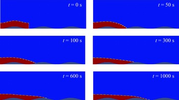
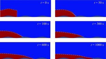
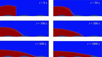


 Open access