


1. Introduction
A fundamental challenge in fluid dynamics research is the identification of appropriate scaling laws for the turbulence properties. In wall turbulence, the classical scaling for the velocity fluctuations is based on the friction velocity, namely  $u_{\tau } = (\tau _w/\rho )^{1/2}$, where $\tau _w$ is the wall shear stress, and $\rho$ is the fluid density. Two length scales can instead be identified, namely the viscous (inner) length scale $\delta _v = \nu / u_{\tau }$ (with $\nu$ the fluid kinematic viscosity), and the outer length scale, say $\delta$, connected with the global dimensions of the wall layer. This classical scenario, first envisaged by Prandtl (Reference Prandtl1925), was challenged by later experimental and numerical data (Spalart Reference Spalart1988; DeGraaff & Eaton Reference DeGraaff and Eaton2000; Marusic Reference Marusic2001; Metzger & Klewicki Reference Metzger and Klewicki2001, to mention a few), which showed that the inner-scaled wall-parallel velocity variances have a clear Reynolds-number dependence. A theoretical layout to explain violations from strict inner-layer universality was set by Townsend (Reference Townsend1976), through the so-called attached-eddy model, hereafter referred to as AEM. The model appeals to the existence of a self-similar hierarchy of eddies rooted at the wall, which, on account of the impermeability condition, can only convey wall-parallel velocity fluctuations in the wall proximity, thus retaining a footprint which manifests itself with superposition and modulation effects (Hutchins & Marusic Reference Hutchins and Marusic2007b; Mathis, Hutchins & Marusic Reference Mathis, Hutchins and Marusic2009). The AEM and its subsequent extensions (Perry & Chong Reference Perry and Chong1982; Perry, Henbest & Chong Reference Perry, Henbest and Chong1986; Perry & Marusic Reference Perry and Marusic1995; Marusic & Monty Reference Marusic and Monty2019) currently constitute the most complete theoretical framework to explain the distributions of the statistical properties in wall turbulence. One key prediction of the AEM is that the inner-scaled wall-parallel velocity variances at a fixed outer-scaled location should decrease logarithmically with the wall distance (Townsend Reference Townsend1976; Perry & Chong Reference Perry and Chong1982; Meneveau & Marusic Reference Meneveau and Marusic2013). A weaker corollary of the model (Marusic, Baars & Hutchins Reference Marusic, Baars and Hutchins2017; Baars & Marusic Reference Baars and Marusic2020b) is that the inner-scaled velocity variances at fixed $y^+$ (hereafter, the ‘ $+$’ superscript refers to inner normalization) in the inner part of the wall layer should increase logarithmically with ${{Re}}_{\tau }$, where ${{Re}}_{\tau } = \delta / \delta _v = u_{\tau } \delta / \nu$, is the friction Reynolds number. If true, this corollary would imply that strict wall scaling is violated.
At least one potential weakness may be envisaged in applying the AEM to asymptotically high  ${{Re}}_{\tau }$. If the growth of the buffer-layer peak of the streamwise velocity variance were to persist indefinitely, and if the peak consistently occurred at the same position ( $\kern 1.5pt y^+ \approx 15$, see Sreenivasan Reference Sreenivasan1989), it would lead to an increasingly high probability of instantaneous negative velocity events. This would likely alter the nature of the flow. Whereas the possibility of instantaneous velocity reversal in the viscous sublayer is known (Lenaers et al. Reference Lenaers, Li, Brethouwer, Schlatter and Örlü2012), it is hard to believe that this can extend to the buffer layer. In fact, an alternative scenario has been recently advocated by Chen & Sreenivasan (Reference Chen and Sreenivasan2021), whereby growth of the buffer-layer peak would saturate on account of a bound on the dissipation rate of the streamwise velocity variance. This would in turn imply that the wall-parallel velocity variances follow a defect power-law dependence with the wall distance, rather than logarithmic. Eventually, strict wall scaling would be restored in the limit of very high Reynolds numbers. Although the model of Chen & Sreenivasan (Reference Chen and Sreenivasan2021) lacks at the moment solid mathematical foundations, it nevertheless seems to comply with existing direct numerical simulation (DNS) and experimental data at least as well as the classical AEM. Hence, it has stirred the interest of the community, stimulating a number of follow-up studies (Chen & Sreenivasan Reference Chen and Sreenivasan2022; Klewicki Reference Klewicki2022; Monkewitz Reference Monkewitz2022, Reference Monkewitz2023; Hwang Reference Hwang2024; Nagib, Monkewitz & Sreenivasan Reference Nagib, Monkewitz and Sreenivasan2024). A common conclusion drawn from those studies appears to be that discerning alternative scaling based solely on inspection of basic statistics, such as velocity variances, requires access to Reynolds numbers that are well beyond the capabilities of current and possibly future experimental and numerical approaches.
The key objective of this paper is showing that some insight into the asymptotic behaviour of turbulence in the near-wall region can in fact be achieved even with current day data. For this purpose, we examine the velocity spectra obtained from a newly generated DNS dataset of turbulent pipe flow, reaching Reynolds numbers up to  ${{Re}}_{\tau } \approx 12\,000$, based on which we believe that informed extrapolation is possible.
2. The DNS database
This paper extends upon a previous publication on the subject, where Reynolds numbers up to  ${{Re}}_{\tau } \approx 6000$ were achieved (Pirozzoli et al. Reference Pirozzoli, Romero, Fatica, Verzicco and Orlandi2021). Here, the database is enlarged and improved, by extending the time interval of previous DNS, and including a new data point at ${{Re}}_{\tau } \approx 12000$. A list of the flow cases is reported in table 1, which includes basic information about the computational mesh and some key parameters. The numerical algorithm is the same as in Pirozzoli et al. (Reference Pirozzoli, Romero, Fatica, Verzicco and Orlandi2021), and details on the mesh resolution are provided in Appendix A. As one can see in table 1, the largest DNS has run for less than ten eddy turnover times, which is the commonly accepted limit to guarantee time convergence (Hoyas & Jiménez Reference Hoyas and Jiménez2006). Nevertheless, careful examination of the time convergence according to the method of Russo & Luchini (Reference Russo and Luchini2017) has shown that the estimated standard deviation in the prediction of the streamwise velocity variance in the range of wall distances under scrutiny here ( $\kern 1.5pt y^+ \leqslant 400$), is at most $0.6\,\%$. Uncertainty is obviously larger in the velocity spectra, for which confidence bands are provided, see e.g. figure 3. Essential details regarding the mean velocity profiles are provided in Appendix B; however, a comprehensive overview of the DNS results will be presented in future publications. Here, the emphasis is on the spectra of streamwise velocity and the associated variances.
Flow parameters for DNS of pipe flow. Here,  $R$ is the pipe radius, $L_z$ is the pipe axial length, $N_{\theta }$, $N_r$ and $N_z$ are the number of grid points in the azimuthal, radial and axial directions, respectively, ${{Re}}_b = 2 R u_b / \nu$ is the bulk Reynolds number, $f = 8 \tau _w / (\rho u_b^2)$ is the friction factor, ${{Re}}_{\tau } = u_{\tau } R / \nu$ is the friction Reynolds number, $T$ is the time interval used to collect the flow statistics and $\tau _t = R/u_{\tau }$ is the eddy turnover time.

3. Flow organization
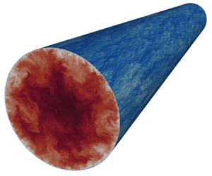
The qualitative structure of flow case G (corresponding to  ${{Re}}_{\tau } \approx 12\,000$) is not dissimilar to what observed in previous publications (Pirozzoli et al. Reference Pirozzoli, Romero, Fatica, Verzicco and Orlandi2021), in that the near-wall region is visually dominated by small-scale streaks whose size scales in inner units, and large-scale streaks scaling on $R$. This is well portrayed in figure 1, which shows the instantaneous streamwise velocity at a distance of fifteen wall units from the wall, each normalized by the corresponding root-mean-square value, at various Reynolds numbers. According to the established scenario (Hutchins & Marusic Reference Hutchins and Marusic2007a), the flow features a two-scale organization, with a large number of small-scale streaks whose typical size scales in inner units, and superposed on those large-scale streaks, being the footprint of ‘superstructures’ (according to the original definition of Hutchins & Marusic Reference Hutchins and Marusic2007a), whose size is instead proportional to $R$. Hence, whereas the former become vanishingly small as ${{Re}}_{\tau }$ increases, the size of the latter is visually unaffected. Careful inspection of the figures further suggests that the superstructures seem to be most intense at the lowest Reynolds number under consideration, whereas their strength seems to slightly decline at higher ${{Re}}_{\tau }$. This observation would imply that the near-wall influence of the superstructures, which are rooted in the outer layer, slightly decreases with the Reynolds number, to an extent that we will attempt to quantify in this manuscript.
Normalized streamwise velocity fluctuations ( $u/\sqrt {\langle u^2 \rangle }$), at $y^+ = 15$. Thirty-two contours are shown, from $-3$ to $3$, in colour scale from blue to red.

Figure 2 shows the spectral maps for the streamwise velocity field, namely the spectral densities ( $E_u$), presented as a function of the wall distance ( $\kern 1.5pt y$) and of the spanwise wavelength ( $\lambda _{\theta }$), pre-multiplied by $k_{\theta }=2 {\rm \pi}/ \lambda _{\theta }$. The figure highlights the near universality of the small scales of motion, with a prominent buffer-layer peak which is universal in inner wall units, and an outer energetic site featuring $R$-sized very large-scale motions previously observed in experiments (Kim & Adrian Reference Kim and Adrian1999; Hellström & Smits Reference Hellström and Smits2014), and which correspond to the superstructures for the present flow. Between the two primary locations, a band of energetic intermediate modes is observed, with lengths roughly proportional to their distance from the wall, aligning with the AEM (Hwang Reference Hwang2015). The discrepancy between the two sites, in terms of both physical distance and of eddy size, increases in proportion to ${{Re}}_{\tau }$, reaching approximately two orders of magnitude in flow case G. The figure also well clarifies that the influence of the attached eddies and of the $O(R)$ eddies on streamwise velocity fluctuations extends down to the wall. Indeed, based on dimensional arguments, spectral densities in the attached-eddy region are expected to depend on $\lambda _{\theta }/y$, hence the corresponding iso-lines are expected to occur in bands parallel to the main energetic ridge, which we highlight with a diagonal line in panel (G). While this is approximately true in the region above the main ridge, the spectral iso-lines rather tend to attain a triangular shape in the region between the spectral ridge and the wall, as a result of energy ‘leakage’ from the overlying eddies. This region under the influence of wall-attached eddies is tentatively marked with dashed red lines in figure 2G, showing that an upper value of the wall distance exists past which the influence of outer eddies is not felt. Setting the maximum wavelength of the attached eddies to $\lambda _{\theta } = 0.4 R$, it turns out that the maximum wall distance at which their influence is felt is $y_{\textit{max} }^+ \approx 0.0044 \, {{Re}}_{\tau }$, with $y_{\textit{max} }^+ \approx 530$ at the highest Reynolds number under scrutiny here. This ‘near-wall’ region is the main subject of investigation in the present study.
Variation of pre-multiplied spanwise spectral densities of fluctuating streamwise velocity with wall distance. Wall distances and wavelengths are reported both in inner units (bottom, left axes), and in outer units (top, right axes). In G the diagonal line denotes the trend  $y^+ = 0.11 \lambda _{\theta }^+$, and the trapezoidal region bounded by the red dashed line marks the region of near-wall influence of attached eddies. Contour levels from 0.36 to 3.6 are shown, in intervals of 0.36.

4. The spectra of streamwise velocity
Previous models of the velocity spectra in turbulent wall layers are mainly based on the work of Perry et al. (Reference Perry, Henbest and Chong1986). The key idea is that, away from the wall, in the inviscid-dominated region, the spectra can be distinguished in three regions: the range of dissipative eddies, scaling in inner units, the region of the  $\delta$-sized eddies (here, $R$-sized), scaling in outer units, and a range of wall-attached eddies, for which the relevant length scale is the wall distance. In this region, under the crucial assumption that the population density of eddies that varies inversely with size and hence with distance from the wall, Perry et al. (Reference Perry, Henbest and Chong1986) predicted the occurrence of a $k^{-1}$ spectral range, where $k$ is any wall-parallel wavenumber. Integration of the resulting spectra yields the prediction, consistent with the phenomenological theory of Townsend (Reference Townsend1976), that the streamwise velocity variance should decay logarithmically with the outer-scaled wall distance in the region of the wall layer controlled by the attached eddies. Whereas this scenario is qualitatively confirmed in the spectral maps obtained from experiments and DNS, quantitative evidence for the $k^{-1}$ spectral range is quite scarce (Vallikivi, Ganapathisubramani & Smits Reference Vallikivi, Ganapathisubramani and Smits2015; Baars & Marusic Reference Baars and Marusic2020a), and the original authors (Perry et al. Reference Perry, Henbest and Chong1986) also observed deviations from the expected trend. Marusic & Monty (Reference Marusic and Monty2019) and Baars & Marusic (Reference Baars and Marusic2020a) noted that limited Reynolds numbers could be a reason for failure in observing the expected scaling. In any case, it is not quite clear why and how the spectral scaling in the outer, inviscid-dominated region should reflect the near-wall region in which the peak velocity variance occurs, since viscous effects can be non-negligible (Hwang Reference Hwang2016). Arguments for why this should be the case were, nonetheless, offered by Marusic et al. (Reference Marusic, Baars and Hutchins2017); Baars & Marusic (Reference Baars and Marusic2020b).
In figure 3 we show the spanwise spectral densities of streamwise velocity fluctuations at a number of locations at fixed  $y^+ < y_{max}^+$. Uncertainty bars are reported in grey shades in the left-hand side panels for flow case G, showing that the effects of limited time convergence are mainly concentrated at scales $\lambda _{\theta } \gtrsim R$. The figure provides clear evidence that universality of the spectra at the small scales is achieved when inner scaling is used, at least for ${{Re}}_{\tau } \gtrsim 2000$. Furthermore, this universal inner-scaled layer tends to become more and more extended towards longer wavelengths as ${{Re}}_{\tau }$ increases, until transition occurs to a $R$-scaled spectral range. No clear evidence for a definite $k_{\theta }^{-1}$ spectral range is observed, which in the pre-multiplied representation would correspond to a plateau region. Careful inspection of the velocity spectra in log–log representation (see the right-hand side panels) rather suggests the existence of a range of wavelengths with negative power-law behaviour.
Pre-multiplied spanwise spectral densities of streamwise velocity at various wall distances:  $y^+=1$ (a,b), $y^+=15$ (c,d), $y^+=50$ (e,f), $y^+=100$ (g,h), $y^+=200$ (i,j), $y^+=400$ (k,l). A semi-log representation is used in the left-hand side panels, and a log–log representation is used in the right-hand side panels. The shaded grey regions in the left-hand side panels denote the expected range of uncertainty for flow case G. The dashed grey lines in the right-hand side panels mark the trend $\lambda_{\theta}^{-0.18}$. The colour codes are as in table 1.

Standard overlap arguments such as those used by Millikan (Reference Millikan1938) to infer the behaviour of the mean velocity profile in wall-bounded flows can also be applied to determine the plausible structure of the velocity spectra, by assuming that: (i) the typical velocity of all eddies is the friction velocity and (ii) the typical length of the small eddies is  $\delta _v$, whereas the typical length of the large eddies is $R$. The transition (overlap) layer between the inner- and outer-scaled end of the velocity spectra should then have either the form of a logarithmic law, or of a power law. Based on the DNS data, the second option appears to be more appropriate, and in that case the spectral densities in the overlap layer should behave as
 \begin{equation} k_{\theta}^+ E_u^+ = C \left( \lambda_{\theta}^+ \right)^{-\alpha} = C {{Re}}_{\tau}^{-\alpha} \left( \frac{\lambda_{\theta}}R \right)^{-\alpha}, \end{equation}
holding in inner and outer scaling, respectively, where  $\alpha$ is a possibly universal constant, and $C$ is a constant which in general could depend on $y^+$. Equation (4.1) includes the $k_{\theta }^{-1}$ spectral scaling as a special case, occurring for $\alpha =0$. In that case, both the small-scale end and the large-scale end of the spectrum should be universal.
The DNS data indeed support (4.1), with  $\alpha \approx 0.18 \pm 0.016$, as we have estimated by fitting the DNS data for flow case G in the range of wavelengths $1000 \leqslant \lambda _{\theta }^+ \leqslant 10\,000$. Notably, the power-law exponent is the same at all wall distances and all Reynolds numbers, within the numerical uncertainty. The power-law range is found to be widest at $y^+ = 50$. Closer to the wall, the strong buffer-layer spectral peak tends to mask this range towards the small wavelengths, whereas farther from the wall the region under the influence of attached eddies tends to progressively shrink as $y^+_{max}$ is approached. This is in our opinion a very important observation, which has a number of implications.
To test the universality of the large-scale end of the spectra, in figure 4, the spectral densities are shown as a function of the outer-scaled wavelength. Universality is clearly not as good as seen for the small wavelengths in figure 3, with the energy associated with the large scales of motion becoming slightly but consistently lower at higher Reynolds number, for given  $\lambda _{\theta }/R$. In figure 5 we then show the outer-scaled spectra compensated by ${{Re}}_{\tau }^{\alpha }$, as suggested from (4.1). The figure shows that, with good accuracy, universality at the large-scale end of the spectrum is recovered in a wide range of scales, up to a short-wavelength limit which shifts to the left as ${{Re}}_{\tau }$ increases.
Pre-multiplied spanwise spectral densities of streamwise velocity at various wall distances, reported in outer scaling at  $y^+=1$ (a), $y^+=15$ (b), $y^+=50$ (c), $y^+=100$ (d), $y^+=200$ (e), $y^+=400$ (f). The colour codes are as in table 1.

Pre-multiplied spanwise spectral densities of streamwise velocity at various wall distances, reported in outer scaling and compensated by  ${{Re}}_{\tau }^{0.18}$: $y^+=1$ (a), $y^+=15$ (b), $y^+=50$ (c), $y^+=100$ (d), $y^+=200$ (e), $y^+=400$ (f). The colour codes are as in table 1.

Overall, convincing evidence exists that the small-scale end of the velocity spectra is universal, whereas the large-scale end is not, with an overlap layer connecting the two ends which features a negative power-law behaviour with exponent  $\alpha \approx 0.18$. The same behaviour is also traced in spectra from plane channel flow DNS (Lee & Moser Reference Lee and Moser2015), as shown in Appendix C, which corroborates the generality of our findings.
5. The streamwise velocity variance
The information derived from the analysis of the velocity spectra can be distilled to infer the behaviour of the velocity variance, taking inspiration from Hwang (Reference Hwang2024). Letting  $\lambda _s$ and $\lambda _{\ell }$, respectively, indicate the lower and upper limits for the observed overlap spectral range, the velocity variance can be expressed as
 \begin{equation} \left\langle u^2 \right\rangle^+ = \underbrace{\int_{0}^{\lambda_s^+} k_{\theta}^+ E_{u,s}^+ \,{\text{d}} \log \lambda_{\theta}^+}_{\langle u^2\rangle^+_s} + \underbrace{\int_{\lambda_s^+}^{\lambda_{\ell}^+} k_{\theta}^+ E_{u,o}^+ \,{\text{d}}\log \lambda_{\theta}^+}_{\langle u^2\rangle^+_o} + \underbrace{\int_{\lambda_{\ell}^+}^{\infty} k_{\theta}^+ E_{u,\ell}^+ \,{\text{d}}\log \lambda_{\theta}^+}_{\langle u^2\rangle^+_{\ell}}, \end{equation}
where the subscripts  $s$,
$s$,  $\ell$ and $o$ denote, respectively, the contributions of the smallest scales, the largest scales and the intermediate, overlap-layer scales. Although the precise values of the limits in (5.1) are not important, it is crucial that the lower limit scales in inner units, hence $\lambda _{s}^+ = {\text {const}}.$, and that the upper limit scales in outer units, hence $\lambda _{\ell }/R = {\text {const}}$. Based on the evidence previously given that the smallest scales tend to be universal across the ${{Re}}_{\tau }$ range, the associated contribution to the velocity variance is also expected to be asymptotically constant, namely
 \begin{equation} \left\langle u^2 \right\rangle^+_s = A_s (y^+). \end{equation}
Since the upper end of the overlap layer should scale in outer units, we further have  $\lambda _{\ell }^+ = {{Re}}_{\tau } \lambda _{\ell }/R \sim {{Re}}_{\tau }$. Based on the matching condition (4.1), and on inspection of figure 5, the contribution from the large scales is then expected to vary as
 \begin{equation} {\left\langle u^2 \right\rangle^+_{\ell}} = B_{\ell} (y^+) \, {{Re}}_{\tau}^{-\alpha} . \end{equation}
This is an especially significant formula implying that imprinting effects imparted by the largest scales of motion (superstructures) on the near-wall region should actually decrease as  ${{Re}}_{\tau }$ increases, in line with observations made by Hwang (Reference Hwang2024). Last, the contribution of the overlap layer can be evaluated by integrating the power-law spectrum given in (4.1), thus obtaining
 \begin{equation} {\left\langle u^2 \right\rangle^+_o} = \frac{C(y^+)}{\alpha} \left[ \left( {\lambda_s^+}\right)^{-\alpha} - \left(\frac{\lambda_{\ell}}{R}\right)^{-\alpha} {{Re}}_{\tau}^{-\alpha} \right] = A_o(y^+) - B_o(y^+) \, {{Re}}_{\tau}^{-\alpha}. \end{equation}
The most important inference of the present analysis is that the overall velocity variance should then vary as
 \begin{equation} \left\langle u^2 \right\rangle^+ = \underbrace{\left( A_s(y^+) + A_o (y^+) \right)}_{A(y^+)} - \underbrace{\left(B_o(y^+) - B_{\ell}(y^+)\right)}_{B(y^+)} {{Re}}_{\tau}^{-\alpha} , \end{equation}
where the functions  $A$ and $B$ do not depend explicitly on the Reynolds number, given the assumptions made to define $\lambda _s$ and $\lambda _{\ell }$. Interestingly, this formula is formally identical to the asymptotic expansion suggested by Monkewitz (Reference Monkewitz2022), in which ${{Re}}_{\tau }^{-\alpha }$ has the role of a gauge function. This formula predicts that, at any fixed $y^+$, the velocity variance should increase, asymptoting to a finite limit as ${{Re}}_{\tau }$ increases, thus restoring strict wall scaling. Values for the asymptotic constants $A$,
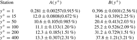
$A$,  $B$ determined from fitting the DNS data at representative off-wall locations are reported in table 2, along with the corresponding standard deviations. The resulting distributions of the streamwise velocity variances as a function of ${{Re}}_{\tau }$ are shown in figure 6. The quality of the fit is quite good, although it tends to deteriorate farther from the wall, since the power-law spectral range becomes narrow, making extrapolations not fully reliable. Most notably, figure 6 shows that, whereas the defect power law could well be mistaken for logarithmic growth at $y^+=15$, the trends at positions farther from the wall are distinctly different from logarithmic. This difference is due to the large contribution conveyed by the smallest eddies close to the wall (recalling figure 3), and tends to overshadow Reynolds-number variations associated with the larger eddies. The reduction of the energetic peak associated with the near-wall streaks occurring farther from the wall makes the actual Reynolds-number dependence manifest. Anyhow, the trend towards the asymptotic limit is quite slow, and even at as extreme Reynolds numbers as ${{Re}}_{\tau }=10^6$, the predicted difference between the velocity variance at $y^+=15$ and its asymptotic value would still be approximately $8\,\%$.
Fitting parameters to use in (5.5), based on DNS data fitting, at several off-wall positions, with accompanying asymptotic standard errors ( $\alpha = 0.18$ is assumed).


The extrapolated distributions of the streamwise velocity variance as a function of the wall distance are shown in figure 7, for various  ${{Re}}_{\tau }$. While confirming that the predictive formula (5.5) covers well the range of Reynolds numbers for which the model is trained, the figure also shows extrapolations beyond that range. Regarding the buffer-layer peak, it is predicted to remain more or less at the same position in inner units, and its maximum amplitude at infinite Reynolds number is predicted to be approximately 12.1. Taking into consideration the uncertainty associated with the parameter $\alpha$, the buffer-layer velocity variance peak is estimated to fall within the range of 11.9 to 12.5. It is worth mentioning that these values are somewhat higher than the value of 11.5 derived from the ${{Re}}_{\tau }^{-0.25}$ defect law (Chen & Sreenivasan Reference Chen and Sreenivasan2021), while Monkewitz (Reference Monkewitz2022) obtained a value of 11.3 through an inner asymptotic expansion informed by DNS data. Farther from the wall, the distribution tends to form a shoulder as ${{Re}}_{\tau }$ increases, with the eventual onset of a clear ‘outer peak’. This outer peak is barely visible at the DNS-accessible Reynolds numbers, but based on the extrapolated data it should attain a higher value than the inner peak at extreme ${{Re}}_{\tau }$.


The primary inquiry revolves around whether the extrapolated distributions agree with experimental measurements. To address this question, in figure 8 we present experimental data collected from various facilities using different measurement techniques. Specifically, particle-image velocimetry (PIV) measurements from the CICLoPE facility (Willert et al. Reference Willert, Soria, Stanislas, Klinner, Amili, Eisfelder, Cuvier, Bellani, Fiorini and Talamelli2017), hot-wire anemometry (HWA) measurements conducted with nanoscale thermal anemometry probes at Princeton's Superpipe facility (Hultmark et al. Reference Hultmark, Vallikivi, Bailey and Smits2012) and laser Doppler velocimetry (LDV) measurements carried out at the Hi-Reff facility in Japan (Ono et al. Reference Ono, Furuichi and Tsuji2023) are included. The comparison reveals highly favourable agreement with all measurements at ’low’ Reynolds numbers, approximately  ${{Re}}_{\tau } \lesssim 5000$. However, notable discrepancies arise at higher Reynolds numbers, varying considerably depending on the set of measurements. Specifically, while alignment remains nearly perfect with the PIV measurements in the CICLoPE facility, the DNS-based extrapolations yield values significantly higher than those obtained from the SuperPipe data. A similar trend of over-prediction of the experimental data is also noticeable, albeit to a lesser degree, when comparing with the LDV measurements in Hi-Reff. In principle, these differences could arise from shortcomings in the DNS and/or its application for extrapolations, but they are more likely associated with issues in the experimental data. Indeed, the three sets of measurements utilized here for reference demonstrate notable discrepancies among each other, suggesting possible filtering effects, particularly for HWA and LDV measurements, whereas PIV measurements might be less affected.
Comparison of streamwise velocity variance distributions predicted from (5.5) (solid lines), with experimental measurements taken at the SuperPipe facility ((b) Hultmark et al. Reference Hultmark, Vallikivi, Bailey and Smits2012), at the CiCLoPE facility ((c) Willert et al. Reference Willert, Soria, Stanislas, Klinner, Amili, Eisfelder, Cuvier, Bellani, Fiorini and Talamelli2017) and at the Hi-Reff facility ((d) Ono, Furuichi & Tsuji Reference Ono, Furuichi and Tsuji2023), at matching values of  ${{Re}}_{\tau }$, as given in the respective legends.

The current analysis also has direct implications for the dissipation rate of the streamwise velocity variance,  $\epsilon _{11} = \nu \langle | \boldsymbol {\nabla } u |^2 \rangle$. As noted by Chen & Sreenivasan (Reference Chen and Sreenivasan2021), at the wall this quantity equals the viscous diffusion term, which in inner units is ${\text {d}}^2 \langle u^2 \rangle ^+ / {\text {d}} {y^+}^2$. The latter quantity (not shown) is virtually indistinguishable from $\langle u^2 \rangle ^+(y^+=1)$, since ${\text {d}}\langle u^2 \rangle ^+ / {\text {d}}y^+ = 0$ at the wall. The inferred trend of $\langle u^2 \rangle ^+(y^+=1)$ (see table 2) then implies that the wall dissipation rate should asymptote to a value of approximately $0.28$, with uncertainty of $\pm 0.01$ on account of variability of $\alpha$. Although a bit higher than the upper bound of $0.25$ advocated by Chen & Sreenivasan (Reference Chen and Sreenivasan2021), and the value of $0.26$ predicted by Monkewitz & Nagib (Reference Monkewitz and Nagib2015) for zero-pressure-gradient boundary layers, this result suggests that wall dissipation retains the same order of magnitude as the maximum production in the buffer layer.
6. Discussion and conclusions
The current analysis, informed by spectral DNS data of turbulent pipe flow up to  ${{Re}}_{\tau } \approx 12\,000$, raises several significant points. Firstly, it offers quantitative arguments, alongside physical intuition, suggesting that strict wall scaling should be restored in the limit of infinite Reynolds numbers. This assertion aligns with propositions put forth in recent literature (Chen & Sreenivasan Reference Chen and Sreenivasan2021; Monkewitz Reference Monkewitz2022), albeit founded on entirely different arguments. In particular, consistent with the assumptions made by Chen & Sreenivasan (Reference Chen and Sreenivasan2021), it appears that the appropriate asymptotic behaviour towards the infinite-Reynolds-number limit follows a defect power law. However, the exponent of this negative power law appears to deviate somewhat from the $\alpha =0.25$ advocated in those studies, being instead closer to $\alpha = 0.18$, with an uncertainty of approximately $\pm 10\,\%$, as revealed by the analysis of the velocity spectra. This discrepancy might stem from the inaccurate assumption made by those authors that the wall dissipation rate should asymptotically approach $0.25$ not to exceed the maximum production rate, although this assertion cannot be rigorously justified on mathematical grounds.
The current analysis fits well within the framework of the classical attached-eddy model. Indeed, the spectrograms reported in figure 2 bear the clear signature of a hierarchy of wall-attached eddies. However, in contrast to the classical formulation of the AEM, we observe that the near-wall signature of these attached eddies becomes fainter as their centre moves away from the wall. This phenomenon is reflected in a spectral decay that is shallower than the traditionally accepted  $k^{-1}$ spectrum derived from inviscid arguments. A secondary implication is that the imprinting of superstructures (here, $R$-sized eddies) on the wall diminishes as ${{Re}}_{\tau }$ increases. However, this observation does not imply that inner-/outer-layer interactions are negligible. Rather, the slow decay rate implies that the influence of outer-layer eddies remains substantial at any reasonably high Reynolds number.
The crucial question revolves around the reason for the spectral slope being less steep than  $k^{-1}$. A plausible explanation is the presence of viscous effects, which impede the flow in the near-wall region. While the AEM treats inactive motions (whose size significantly exceeds the distance from the wall) as satisfying a slip condition at the wall, in reality, they do not. In this regard, the analysis conducted by Spalart (Reference Spalart1988) holds considerable merit. He argued that inactive eddies influence the near-wall region by inducing periodic, low-frequency sloshing motions, leading to the formation of Stokes layers of either laminar or turbulent nature. In the first case, analytical solution of the Navier–Stokes equations with time-periodic change of the free-stream velocity would yield the following form of the streamwise velocity variance (Schlichting & Gersten Reference Schlichting and Gersten2000):
 \begin{equation} \left\langle u^2 \right\rangle^+ \sim 1 + \text{e}^{{-}2 y / \varDelta} - 2 \cos(y/\varDelta) {\text{e}}^{{-}y/\varDelta}, \end{equation}
with  $\varDelta = (2 \nu / \omega )^{1/2}$ the thickness of the Stokes layer, and $\omega$ the oscillation frequency. Bradshaw (Reference Bradshaw1967) proposed a model for turbulent Stokes layers based on the idea that the primary effect of low-frequency inactive motions is a time-periodic change of the wall shear stress, namely $\tau _w = \bar {\tau }_w ( 1 + A \cos (\omega t) )$, with $A \ll 1$. Assuming next that the law-of-the-wall has time to adapt to low-frequency modulation of the wall shear stress results in the following prediction for the velocity variance associated with inactive motions:
 \begin{equation} \left\langle u^2 \right\rangle^+ \sim \left( U^+ + y^+ \frac{{\text{d}} U^+}{{\text{d}} y^+} \right)^2. \end{equation}
These concepts were put to the test by Spalart (Reference Spalart1988), who compared the predictions in (6.1) and (6.2) with the difference in velocity variances at two modest Reynolds numbers, which he used as a proxy for the contribution of inactive motions. Here, both approaches are examined by plotting profiles of  $E_u^+(\lambda _{\theta }^+, y^+)$ for various values of $\lambda _{\theta }^+$, which in the AEM interpretation characterize the intensity of streamwise velocity fluctuations induced by attached eddies centred at a wall distance $y_s^+ \approx 0.11 \lambda _{\theta }^+$ (refer to figure 2).
Figure 9(a) presents a comparison of the spectral density profiles with the prediction given by (6.1), where we have arbitrarily assumed  $\varDelta ^+ = 10$, and attempted to adjust the slope of the DNS data at the wall. While the values of the velocity intensities appear reasonable, the shape is evidently incompatible with the DNS data. On the other hand, figure 9(b) depicts the predictions of (6.2), again after adjusting the near-wall slope. In this case, the agreement with the DNS data is remarkable, particularly for wall distances smaller than the centre of the attached eddies (indicated with bullets in the figure). This observation serves as plausible evidence that turbulent Stokes layers do indeed exist, thereby providing the retardation effects responsible for attenuating the influence of wall-distant eddies.
Flow case G: pre-multiplied spectral density of streamwise velocity as a function of wall distance, corresponding to various wavelengths:  $\lambda _{\theta }^+=455$ ( $\kern 1.5pt y_s^+=50$) (purple), $\lambda _{\theta }^+=909$ ( $\kern 1.5pt y_s^+=100$) (green), ${\lambda _{\theta }^+=3636}$ ( $\kern 1.5pt y_s^+=400$) (orange), $\lambda _{\theta }^+=10970$ ( $\kern 1.5pt y_s^+=1205$) (red). The bullets denote the wall distance of the corresponding eddy centres, see figure 2. The dashed lines in (a) denote predictions of (6.1) with $\varDelta ^+=10$, and in (b) predictions of (6.2).

Although extrapolation is known to be a dangerous, oftentimes ill-posed exercise, we believe that the present observations lay down a sufficiently solid background to project today's DNS results to much higher Reynolds number than feasible in the near or even foreseeable future. When pushed to the extreme, extrapolation of the present data would suggest a scenario where the buffer-layer peak of the streamwise velocity variance, while remaining finite, would be much larger than in any current DNS and experiments, but roughly at the same inner-scaled position. Another important feature which we foresee is a secondary distinct peak farther from the wall, whose strength becomes comparable to and eventually larger than the buffer-layer peak. The primary caution we emphasize is that these predictions rely on the assumption that the observed expansion of the power-law spectrum will persist indefinitely. Should a definite  $k^{-1}$ spectral range arise at higher Reynolds numbers than those achieved thus far in DNS, as suggested by some experimental studies (Baars & Marusic Reference Baars and Marusic2020a), a logarithmic increasing trend would resume. Furthermore, it is important to highlight that the current analysis does not offer an explanation for the specific value of the spectral scaling exponent in the overlap layer. In contrast, Chen & Sreenivasan (Reference Chen and Sreenivasan2021) rationalized the presence of a $-0.25$ exponent in the proposed defect power law by attributing it to the flux of additional energy dissipation from the near-wall region to the outer flow. Thus, further theoretical efforts are still necessary to fully elucidate the observed data and unambiguously establish the asymptotic state of wall turbulence.
Supplementary movie
Supplementary movie is available at https://doi.org/10.1017/jfm.2024.467.
Acknowledgements
Discussions with Y. Hwang, P. Monkewitz, J. Jimenez, A.J. Smits and T. Wei are gratefully appreciated. I acknowledge that the results reported in this paper have been achieved using the EuroHPC Research Infrastructure resource LEONARDO based at CINECA, Casalecchio di Reno, Italy, under a LEAP grant. Constructive criticisms from the anonymous referees are also gratefully acknowledged.
Funding
This research received no specific grant from any funding agency, commercial or not-for-profit sectors.
Declaration of interests
The author reports no conflict of interest.
Data availability statement
The data that support the findings of this study are openly available at the web page http://newton.dma.uniroma1.it/database/.
Appendix A. Box and grid sensitivity analysis
The grid resolution in the axial and azimuthal directions is decided based on previous experience with second-order finite-difference solvers which indicates that grid-independent results are obtained provided  $\Delta x^+ \approx 10$, $R^+ \Delta \theta \approx 4.1$ (Pirozzoli et al. Reference Pirozzoli, Romero, Fatica, Verzicco and Orlandi2021), hence the associated number of grid points is selected as $N_z \approx L_z / R \times {{Re}}_{\tau } / 10$, $N_{\theta } \sim 2 {\rm \pi}\times {{Re}}_{\tau } / 4.1$. The wall-normal distribution of the grid points is designed after the prescriptions set by Pirozzoli & Orlandi (Reference Pirozzoli and Orlandi2021), to resolve the steep near-wall velocity gradients and the local Kolmogorov scale away from the wall, according to
 \begin{equation} y^+(j) = \frac 1{1+(j/j_b)^2} \left[ \Delta y^+_w j + \left( \frac 34 \alpha c_{\eta} j \right)^{4/3} (j/j_b)^2 \right], \end{equation}
where  $\Delta y^+_w=0.05$ is the wall distance of the first grid point, $j_b=40$ defines the grid index at which transition between the near-wall and the outer mesh stretching takes place and $c_{\eta }=0.8$ guarantees resolution of wavenumbers up to $k_{max} \eta = 1.5$, with $\eta$ the local Kolmogorov length scale. The distributions of the grid points for the DNS listed in table 1 are shown in figure 10(a). A slightly finer mesh is used for flow case G than for the other cases. The wall-normal resolution is verified a posteriori in figure 10(b), where we show the grid spacing expressed in local Kolmogorov units, which is found to be no larger than $2.2$ throughout the radial direction.
(a) Distribution of wall-normal grid coordinates as a function of grid index ( $\kern 1.5pt j$), and (b) corresponding grid spacings expressed in Kolmogorov units. The colour codes are as in table 1.

The sensitivity of the computed results to the computational box size and grid resolution has been assessed through additional simulations conducted at  ${{Re}}_b = 44\,000$ (flow case C), as listed in table 1. Specifically, we have doubled the number of points in the radial direction (flow case C-FY) and doubled and tripled the pipe length (flow cases C-L and C-LL, respectively). All these flow cases have been simulated for numerous eddy turnover times, for the purpose of removing the time sampling error. The resulting change in the one-point statistics is well below $1\,\%$, as illustrated in figure 11, even for flow properties that are challenging to converge over time, such as the log-law indicator function (Hoyas et al. Reference Hoyas, Vinuesa, Baxerres and Nagib2024). Figure 12 additionally presents a comparison of the pre-multiplied spanwise spectra at several off-wall positions for the same flow cases. Once again, box and grid independence is demonstrated to be excellent, indicating that uncertainties primarily stem from finite time sampling.
Box and grid sensitivity study for one-point statistics: (a) inner-scaled mean velocity profiles and streamwise velocity variances, (b) log-law diagnostics function, (c) velocity variances. Flow cases C, C-FY, C-L, C-LL are shown, see table 1 for the line style.

Box and grid sensitivity study for pre-multiplied spanwise spectral densities of streamwise velocity at various wall distances:  $y^+=1$ (a), $y^+=15$ (b), $y^+=50$ (c), $y^+=100$ (d), $y^+=200$ (e), $y^+=400$ (f). Flow cases C, C-FY, C-L, C-LL are shown, see table 1 for the line style.

Appendix B. Mean velocity profiles
The mean velocity profiles for the DNS cases listed in table 1 are presented in figure 13(a), accompanied by the associated log-law diagnostic functions shown in panel (b). The latter quantity is commonly used to verify the presence of a genuine logarithmic layer in the mean velocity profile, which would be indicated by a plateau. This diagnostic function exhibits two peaks: one corresponding to the buffer layer, which is nearly universal in inner scaling at  ${{Re}}_{\tau } \gtrsim 10^3$, and an outer peak corresponding to the wake region, which also becomes approximately universal in inner units. Between these two regions, the distribution tends to change significantly with the Reynolds number. While previous DNS and analyses suggested linear deviations from the logarithmic behaviour (Afzal & Yajnik Reference Afzal and Yajnik1973; Jiménez & Moser Reference Jiménez and Moser2007; Luchini Reference Luchini2017; Pirozzoli et al. Reference Pirozzoli, Romero, Fatica, Verzicco and Orlandi2021), at the highest Reynolds number achieved in this study, the onset of a genuine logarithmic layer is observed, starting at $y^+ \approx 500$ and extending up to $y/R \approx 0.2$. This finding is consistent with the SuperPipe data (symbols in panel (b)), recent DNS of plane channel flow (Hoyas et al. Reference Hoyas, Oberlack, Alcántara-Ávila, Kraheberger and Laux2022) and is in line with the theoretical analysis of Monkewitz (Reference Monkewitz2021). The data support a value of the Kármán constant of $\kappa \approx 0.38$, slightly less than estimated in previous studies, in which, however, a genuine logarithmic layer was not observed. The figure reveals a large scatter associated with limited time convergence of flow case D for this indicator, confirming recent analyses (Hoyas et al. Reference Hoyas, Vinuesa, Baxerres and Nagib2024). While the predictions for the inner layer appear to be robust, much longer integration times are required to achieve satisfactory convergence of statistics associated with velocity derivatives. However, achieving such convergence is currently beyond the capabilities of DNS. Figure 13(a) confirms that the mean velocity profiles tend to cluster around a common logarithmic distribution. The DNS velocity profiles for ${{Re}}_{\tau } \geqslant 10^3$ follow this distribution with deviations of no more than $0.1$ inner units from $y^+ \approx 30$ to $y/R \approx 0.15$, where the core region develops.
Inner-scaled mean velocity profiles obtained from DNS are presented in panel (a), along with the corresponding log-law diagnostic function shown in panel (b). In panel (a), the dashed line represents the logarithmic fit  $U_{\log }^+ = \log y^+ / 0.38 + 4.3$. In panel (b), the dashed horizontal line denotes the inverse of the expected Kármán constant, $\kappa = 0.38$, while symbols denote Princeton SuperPipe data (McKeon, Zagarola & Smits Reference McKeon, Zagarola and Smits2005) at ${{Re}}_{\tau } = 1825, 3328, 6617, 10914$. The shaded grey regions denote the expected range of uncertainty for flow case G (not visible in panel (a)). Colour codes for the lines are as described in table 1.

Appendix C. Comparison with DNS of channel flow
In figure 14, we present the spanwise spectra of the streamwise velocity obtained from the channel flow DNS conducted by Lee & Moser (Reference Lee and Moser2015), at several off-wall locations, while maintaining a constant  $y^+$. This figure offers clear evidence that universality of the spectra at small scales is achieved when inner scaling is employed, at least for ${{Re}}_{\tau } \gtrsim 2000$. Furthermore, this universal inner-scaled layer tends to become more extended towards longer wavelengths as ${{Re}}_{\tau }$ increases, until a transition to an $h$-scaled spectral range occurs. These distributions support the findings reported in figure 3, indicating that the premultiplied spectra at all considered wall distances exhibit a negative power-law range, with an exponent of approximately $0.18$, as for pipe flow. However, due to the more limited range of available Reynolds numbers, a clear power-law behaviour is visible only up to $y^+ \approx 100$. Similar to our analysis for pipe flow, figure 15(a) illustrates the Reynolds-number trends of the velocity variance at various distances from the wall. This figure reaffirms the accuracy of (5.5) in fitting the DNS data and visually highlights deviations from a logarithmic behaviour.
Pre-multiplied spanwise spectral densities of streamwise velocity from DNS of channel flow (Lee & Moser Reference Lee and Moser2015), at various wall distances:  $y^+=1$ (a,b), $y^+=15$ (c,d), $y^+=50$ (e,f), $y^+=100$ (g,h), $y^+=200$ (i,j), $y^+=400$ (k,l). A semi-log representation is used in the left-hand side panels, and a log–log representation is used in the right-hand side panels. The dashed grey lines in the right-hand side panels mark the trend $\lambda_{\theta}^{-0.18}$. The colour codes correspond to Reynolds numbers ${{Re}}_{\tau } =180$ (blue), 550 (green), 1000 (cyan), 2000 (orange), 5200 (purple).

Analysis of velocity variance for turbulent channel flow (Lee & Moser Reference Lee and Moser2015). (a) Streamwise velocity variances (symbols) as a function of  ${{Re}}_{\tau }$ at various off-wall positions, along with corresponding fits according to (5.5); and (b) predicted wall-normal distributions of streamwise velocity variances at various ${{Re}}_{\tau }$, again according to (5.5). In panel (b), the symbols denote the DNS data used to determine the fit coefficients $A(y^+)$ and $B(y^+)$, with colour codes corresponding to ${{Re}}_{\tau } = 550$ (green), 1000 (cyan), 2000 (orange) and 5200 (purple).

Figure 15(b) depicts the resulting extrapolated distributions at extreme Reynolds numbers. The outcome is qualitatively very similar to that shown in figure 7 for pipe flow, demonstrating saturation of the buffer-layer peak and the onset of a dominant outer-layer peak. We estimate that the asymptotic value of the buffer-layer peak is approximately  $12.3$, while the wall dissipation should asymptote to about $0.27$, which aligns well with the numerical values determined for pipe flow.


 Open access