


1. Introduction
Multiphase flows are fundamental in numerous natural and industrial processes, ranging from atmospheric phenomena to chemical reactors and heat exchangers (Tryggvason, Scardovelli & Zaleski Reference Tryggvason, Scardovelli and Zaleski2011; Kure, Jakobsen & Solsvik Reference Kure, Jakobsen and Solsvik2024). Of particular interest are fluids such as molten salts and liquid metals (e.g. liquid lead and sodium) that are characterised by low Prandtl number $Pr$
(Bricteux et al. Reference Bricteux, Duponcheel, Manconi and Bartosiewicz2012) – where the Prandtl number represents the ratio of momentum diffusivity to thermal diffusivity. These fluids play an important role in different disciplines. In astrophysical fluid dynamics, laboratory experiments with liquid metals replicate the magnetohydrodynamic processes governing angular momentum transport in accretion disks (Schindler et al. Reference Schindler, Eckert, Zürner, Schumacher and Vogt2022; Vernet, Fauve & Gissinger Reference Vernet, Fauve and Gissinger2022). In industrial contexts, such as converter steelmaking, high-velocity oxygen jets are injected into molten steel to oxidise impurities such as carbon and silicon. This process generates intense turbulence, gas–liquid slag interactions, and thermal gradients that dictate process efficiency and final alloy properties (Wang et al. Reference Wang, Cao, Vanierschot, Cheng, Blanpain and Guo2020; Chang et al. Reference Chang, Zou, Liu, Isac, Cao, Su and Guthrie2021). Similarly, the production of metallic foams relies on injecting gas bubbles into molten metal column reactors, where the interplay between bubble coalescence, drainage and solidification governs foam porosity (Banhart Reference Banhart2001). In energy storage systems, liquid metal batteries – such as sodium-zinc (Na–Zn) systems – leverage stratified layers of immiscible molten metals to achieve high current densities and rapid charge–discharge cycles (Kelley & Weier Reference Kelley and Weier2018; Davidson et al. Reference Davidson, Wong, Atkinson and Ranjan2022; Duczek et al. Reference Duczek2024). Likewise, in fusion and nuclear technologies, liquid metal divertors face complex multiphase interactions with plasma particles (Mirnov, Dem’yanenko & Murav’ev Reference Mirnov, Dem’yanenko and Murav’ev1992; Fisher, Sun & Kolemen Reference Fisher, Sun and Kolemen2020), and in nuclear reactors, liquid metals and molten salts serve as coolants due to their excellent heat transfer properties (Jeltsov Reference Jeltsov2018; Bhushan et al. Reference Bhushan, Elmellouki, Walters, Hassan, Merzari and Obabko2022; Tai et al. Reference Tai, Nguyen, Iskhakov, Merzari, Dinh and Bolotnov2024).
$Pr$
(Bricteux et al. Reference Bricteux, Duponcheel, Manconi and Bartosiewicz2012) – where the Prandtl number represents the ratio of momentum diffusivity to thermal diffusivity. These fluids play an important role in different disciplines. In astrophysical fluid dynamics, laboratory experiments with liquid metals replicate the magnetohydrodynamic processes governing angular momentum transport in accretion disks (Schindler et al. Reference Schindler, Eckert, Zürner, Schumacher and Vogt2022; Vernet, Fauve & Gissinger Reference Vernet, Fauve and Gissinger2022). In industrial contexts, such as converter steelmaking, high-velocity oxygen jets are injected into molten steel to oxidise impurities such as carbon and silicon. This process generates intense turbulence, gas–liquid slag interactions, and thermal gradients that dictate process efficiency and final alloy properties (Wang et al. Reference Wang, Cao, Vanierschot, Cheng, Blanpain and Guo2020; Chang et al. Reference Chang, Zou, Liu, Isac, Cao, Su and Guthrie2021). Similarly, the production of metallic foams relies on injecting gas bubbles into molten metal column reactors, where the interplay between bubble coalescence, drainage and solidification governs foam porosity (Banhart Reference Banhart2001). In energy storage systems, liquid metal batteries – such as sodium-zinc (Na–Zn) systems – leverage stratified layers of immiscible molten metals to achieve high current densities and rapid charge–discharge cycles (Kelley & Weier Reference Kelley and Weier2018; Davidson et al. Reference Davidson, Wong, Atkinson and Ranjan2022; Duczek et al. Reference Duczek2024). Likewise, in fusion and nuclear technologies, liquid metal divertors face complex multiphase interactions with plasma particles (Mirnov, Dem’yanenko & Murav’ev Reference Mirnov, Dem’yanenko and Murav’ev1992; Fisher, Sun & Kolemen Reference Fisher, Sun and Kolemen2020), and in nuclear reactors, liquid metals and molten salts serve as coolants due to their excellent heat transfer properties (Jeltsov Reference Jeltsov2018; Bhushan et al. Reference Bhushan, Elmellouki, Walters, Hassan, Merzari and Obabko2022; Tai et al. Reference Tai, Nguyen, Iskhakov, Merzari, Dinh and Bolotnov2024).
Due to the complexity that a multiphase flow adds to the problem, previous works have mostly focused on canonical single-phase configurations. The pioneering study by Kim & Moin (Reference Kim and Moin1989) was the first to perform direct numerical simulations (DNS) of a channel flow considering also the evolution of the thermal field and investigating $Pr=0.1,0.7,2$
. Building on this seminal work, subsequent studies expanded the parameter range, examining both higher and lower
$Pr=0.1,0.7,2$
. Building on this seminal work, subsequent studies expanded the parameter range, examining both higher and lower $Pr$
values (Kasagi, Tomita & Kuroda Reference Kasagi, Tomita and Kuroda1993; Kawamura et al. Reference Kawamura, Ohsaka, Abe and Yamamoto1998; Na, Papavassiliou & Hanratty Reference Na, Papavassiliou and Hanratty1999; Piller, Nobile & Hanratty Reference Piller, Nobile and Hanratty2002; Abe, Kawamura & Matsuo Reference Abe, Kawamura and Matsuo2004; Orlandi & Leonardi Reference Orlandi and Leonardi2004; Pirozzoli, Bernardini & Orlandi Reference Pirozzoli, Bernardini and Orlandi2016; Scheel & Schumacher Reference Scheel and Schumacher2016; Lluesma-Rodríguez et al. Reference Lluesma-Rodríguez, Hoyas and Perez-Quiles2018; Alcántara-Ávila & Hoyas Reference Alcántara-Ávila and Hoyas2021). These simulations highlighted that for
$Pr$
values (Kasagi, Tomita & Kuroda Reference Kasagi, Tomita and Kuroda1993; Kawamura et al. Reference Kawamura, Ohsaka, Abe and Yamamoto1998; Na, Papavassiliou & Hanratty Reference Na, Papavassiliou and Hanratty1999; Piller, Nobile & Hanratty Reference Piller, Nobile and Hanratty2002; Abe, Kawamura & Matsuo Reference Abe, Kawamura and Matsuo2004; Orlandi & Leonardi Reference Orlandi and Leonardi2004; Pirozzoli, Bernardini & Orlandi Reference Pirozzoli, Bernardini and Orlandi2016; Scheel & Schumacher Reference Scheel and Schumacher2016; Lluesma-Rodríguez et al. Reference Lluesma-Rodríguez, Hoyas and Perez-Quiles2018; Alcántara-Ávila & Hoyas Reference Alcántara-Ávila and Hoyas2021). These simulations highlighted that for $Pr \approx 1$
, the velocity and temperature profiles are strongly correlated. Conversely, for simulations at
$Pr \approx 1$
, the velocity and temperature profiles are strongly correlated. Conversely, for simulations at $Pr \ll 1$
, where thermal diffusion dominates over viscous effects, the thermal boundary layer becomes thicker than the viscous boundary layer. Laminar-like thermal boundary layers, extending across the entire channel width, have been reported in numerical simulations, with experimental results confirming these findings (Lefhalm et al. Reference Lefhalm, Tak, Piecha and Stieglitz2004; Schulenberg & Stieglitz Reference Schulenberg and Stieglitz2010; Razuvanov et al. Reference Razuvanov, Frick, Belyaev and Sviridov2019, Reference Razuvanov, Pyatnitskaya, Frick, Belyaev and Sviridov2020; Kim et al. Reference Kim, Schindler, Vogt and Eckert2024).
$Pr \ll 1$
, where thermal diffusion dominates over viscous effects, the thermal boundary layer becomes thicker than the viscous boundary layer. Laminar-like thermal boundary layers, extending across the entire channel width, have been reported in numerical simulations, with experimental results confirming these findings (Lefhalm et al. Reference Lefhalm, Tak, Piecha and Stieglitz2004; Schulenberg & Stieglitz Reference Schulenberg and Stieglitz2010; Razuvanov et al. Reference Razuvanov, Frick, Belyaev and Sviridov2019, Reference Razuvanov, Pyatnitskaya, Frick, Belyaev and Sviridov2020; Kim et al. Reference Kim, Schindler, Vogt and Eckert2024).
In recent years, thanks to the increased computational power available and the development of accurate numerical methodologies, heat transfer in multiphase flows has attracted more attention and has been investigated using the DNS approach. Drops/bubbles with a sub-Kolmogorov diameter size can be investigated using the point-particle assumption (Elghobashi Reference Elghobashi2019). In this framework, the dispersed phase is tracked with a Lagrangian approach, while the temperature is solved with an Eulerian approach (Russo et al. Reference Russo, Kuerten, van der Geld and Geurts2014; Kuerten & Vreman Reference Kuerten and Vreman2015; Ardekani et al. Reference Ardekani, Abouali, Picano and Brandt2018). On the contrary, when the diameter of the drops/bubbles is larger than the Kolmogorov scale, the finite size effect of the drop/bubble, its deformability and the topological changes of the interface – coalescence and breakage – cannot be neglected. As a consequence, recently considerable effort has been put into analysing heat transport in multiphase flows using interface-resolved simulations (Zhong, Funfschilling & Ahlers Reference Zhong, Funfschilling and Ahlers2009; Dabiri & Tryggvason Reference Dabiri and Tryggvason2015; Soligo, Roccon & Soldati Reference Soligo, Roccon and Soldati2021; Liu et al. Reference Liu, Chong, Ng, Verzicco and Lohse2022a , Reference Liu, Chong, Yang, Verzicco and Lohse b ; Dung et al. Reference Dung, Waasdorp, Sun, Lohse and Huisman2023; Hidman et al. Reference Hidman, Ström, Sasic and Sardina2023; Bilondi et al. Reference Bilondi, Scapin, Brandt and Mirbod2024; Mangani et al. Reference Mangani, Roccon, Zonta and Soldati2024).
Despite recent works, research on low- $Pr$
multiphase systems remains scarce. In this work, we perform DNS to investigate how the injection of a swarm of large and deformable drops into a turbulent channel flow modifies the heat transfer process. The carrier phase is characterised by fixed Prandtl number
$Pr$
multiphase systems remains scarce. In this work, we perform DNS to investigate how the injection of a swarm of large and deformable drops into a turbulent channel flow modifies the heat transfer process. The carrier phase is characterised by fixed Prandtl number $Pr_c=0.013$
, representative of realistic low-
$Pr_c=0.013$
, representative of realistic low- $Pr$
fluids such as liquid metals. The dispersed phase, however, spans a range of
$Pr$
fluids such as liquid metals. The dispersed phase, however, spans a range of $Pr_d$
values from
$Pr_d$
values from $0.013$
up to
$0.013$
up to $7$
. Using these simulations, we investigate the impact of droplets on temperature statistics, highlighting the interplay between carrier and dispersed phase thermal dynamics. By analysing global heat transfer, we assess how droplet introduction influences heat transfer dynamics in both phases. In addition, we identify the governing physical mechanisms, and propose a phenomenological model that accurately describes heat transfer performance as a function of the dispersed phase Prandtl number and volume fraction.
$7$
. Using these simulations, we investigate the impact of droplets on temperature statistics, highlighting the interplay between carrier and dispersed phase thermal dynamics. By analysing global heat transfer, we assess how droplet introduction influences heat transfer dynamics in both phases. In addition, we identify the governing physical mechanisms, and propose a phenomenological model that accurately describes heat transfer performance as a function of the dispersed phase Prandtl number and volume fraction.
The paper is organised as follows. Section 2 presents the governing equations, numerical methodology and simulation set-up. In § 3, we begin with qualitative observations before delving into the statistical characterisation of temperature fields, both globally and within the carrier and dispersed phases. Then we provide a detailed analysis of the heat flux in the wall-normal direction, introducing and validating the proposed scaling law. Finally, § 4 concludes with a summary of the findings and their implications.
2. Methodology
We perform DNS of channel flow between two differentially heated walls. The coordinate origin is located in the channel centre, with the $x$
-,
$x$
-, $y$
- and
$y$
- and $z$
-axes oriented along the streamwise, spanwise and wall-normal directions, respectively. Denoting the channel half-height as
$z$
-axes oriented along the streamwise, spanwise and wall-normal directions, respectively. Denoting the channel half-height as $h$
, the reference domain dimensions are
$h$
, the reference domain dimensions are $L_x \times L_y \times L_z = 4{\unicode[Arial]{x03C0}} h \times 2{\unicode[Arial]{x03C0}} h \times 2h$
. The flow of two immiscible fluids is modelled using the one-fluid formulation (Prosperetti & Tryggvason Reference Prosperetti and Tryggvason2007; Elghobashi Reference Elghobashi2019), where a single set of continuity, Navier–Stokes and energy equations describes the system hydrodynamics and temperature field. The interface dynamics is captured using a phase-field method. Further details on the numerical framework are provided below.
$L_x \times L_y \times L_z = 4{\unicode[Arial]{x03C0}} h \times 2{\unicode[Arial]{x03C0}} h \times 2h$
. The flow of two immiscible fluids is modelled using the one-fluid formulation (Prosperetti & Tryggvason Reference Prosperetti and Tryggvason2007; Elghobashi Reference Elghobashi2019), where a single set of continuity, Navier–Stokes and energy equations describes the system hydrodynamics and temperature field. The interface dynamics is captured using a phase-field method. Further details on the numerical framework are provided below.
2.1. Phase-field method
The phase-field method is an interface-capturing approach (Cahn & Hilliard Reference Cahn and Hilliard1958; Jacqmin Reference Jacqmin1999; Badalassi, Ceniceros & Banerjee Reference Badalassi, Ceniceros and Banerjee2003; Roccon, Zonta & Soldati Reference Roccon, Zonta and Soldati2023) that employs an order parameter, known as the phase-field variable $\phi$
, to distinguish between the two phases. This variable, also referred to as the order parameter, characterises the local concentration of the respective phases. It assumes constant values
$\phi$
, to distinguish between the two phases. This variable, also referred to as the order parameter, characterises the local concentration of the respective phases. It assumes constant values $\phi =-1$
in the carrier phase and
$\phi =-1$
in the carrier phase and $\phi =+1$
in the droplets while it undergoes a smooth transition across the interface. The Cahn–Hilliard equation describes the temporal evolution of the phase-field variable. This equation, in dimensionless form, reads as
$\phi =+1$
in the droplets while it undergoes a smooth transition across the interface. The Cahn–Hilliard equation describes the temporal evolution of the phase-field variable. This equation, in dimensionless form, reads as
 \begin{equation} \frac {\partial \phi }{\partial t} + \boldsymbol{u\cdot \nabla } \phi = \frac {1}{Pe}\nabla ^2\mu _\phi + f_P , \end{equation}
where $\boldsymbol{u}=(u,v,w)$
is the velocity vector,
$\boldsymbol{u}=(u,v,w)$
is the velocity vector, $\textit{Pe}$
is the Péclet number,
$\textit{Pe}$
is the Péclet number, $\mu _\phi$
is the chemical potential, and
$\mu _\phi$
is the chemical potential, and $f_P$
is the penalty flux of the profile-corrected formulation of the phase-field method. The Péclet number
$f_P$
is the penalty flux of the profile-corrected formulation of the phase-field method. The Péclet number $\textit{Pe}$
represents the ratio between the diffusive time scale
$\textit{Pe}$
represents the ratio between the diffusive time scale $h^2/(\mathcal{M}\beta ^2)$
and the convective time scale,
$h^2/(\mathcal{M}\beta ^2)$
and the convective time scale, $h/u_\tau$
:
$h/u_\tau$
:
 \begin{equation} Pe=\frac {u_\tau h}{\mathcal{M}\beta } , \end{equation}
where $u_\tau =\sqrt {\tau _w/\rho _c}$
indicates the friction velocity (
$u_\tau =\sqrt {\tau _w/\rho _c}$
indicates the friction velocity ( $\tau _w$
being the wall-shear stress, and
$\tau _w$
being the wall-shear stress, and $\rho _c$
the density of the carrier fluid),
$\rho _c$
the density of the carrier fluid), $\mathcal{M}$
is the mobility, and
$\mathcal{M}$
is the mobility, and $\beta$
is a positive constant.
$\beta$
is a positive constant.
The chemical potential $\mu _\phi$
is the variational derivative of the Ginzburg–Landau free-energy functional
$\mu _\phi$
is the variational derivative of the Ginzburg–Landau free-energy functional $\mathcal{F}[\phi ,\boldsymbol{\nabla }\phi ]$
. In a system of two immiscible fluids, two terms contribute to the free-energy functional (Ding, Spelt & Shu Reference Ding, Spelt and Shu2007; Soligo, Roccon & Soldati Reference Soligo, Roccon and Soldati2019b
; Schenk et al. Reference Schenk, Giamagas, Roccon, Soldati and Zonta2024):
$\mathcal{F}[\phi ,\boldsymbol{\nabla }\phi ]$
. In a system of two immiscible fluids, two terms contribute to the free-energy functional (Ding, Spelt & Shu Reference Ding, Spelt and Shu2007; Soligo, Roccon & Soldati Reference Soligo, Roccon and Soldati2019b
; Schenk et al. Reference Schenk, Giamagas, Roccon, Soldati and Zonta2024):
 \begin{equation} \mathcal{F}[\phi ,\boldsymbol{\nabla }\phi ]=\int _\Omega (f_0+f_{{mix}})\, {d}\Omega , \end{equation}
where $\Omega$
is the domain considered, and the local term
$\Omega$
is the domain considered, and the local term $f_0$
describes the phobic behaviour of the two fluids that tend to separate into two pure stable phases. Instead, the non-local term,
$f_0$
describes the phobic behaviour of the two fluids that tend to separate into two pure stable phases. Instead, the non-local term, $f_{{mix}}$
, accounts for the energy stored at the interface (surface tension). The resulting expression of the chemical potential is
$f_{{mix}}$
, accounts for the energy stored at the interface (surface tension). The resulting expression of the chemical potential is
 \begin{equation} \mu _\phi =\frac {\delta \mathcal{F}[\phi ,\boldsymbol{\nabla }\phi ]}{\delta \phi }=\phi ^3-\phi -\textit {Ch}^2\,\nabla ^2\phi , \end{equation}
where $\textit {Ch}=\xi /h$
is the Cahn number, which represents the characteristic length scale of the transition layer (
$\textit {Ch}=\xi /h$
is the Cahn number, which represents the characteristic length scale of the transition layer ( $\xi$
being its dimensional value). For a flat interface, it is possible to obtain an analytical solution for the equilibrium profile of the phase-field variable by imposing that the chemical potential is uniform in the system (i.e.
$\xi$
being its dimensional value). For a flat interface, it is possible to obtain an analytical solution for the equilibrium profile of the phase-field variable by imposing that the chemical potential is uniform in the system (i.e. $\boldsymbol{\nabla }\mu _\phi =0$
). The resulting equilibrium profile is
$\boldsymbol{\nabla }\mu _\phi =0$
). The resulting equilibrium profile is
 \begin{equation} \phi _{{eq}}=\tanh \left (\frac {s}{\sqrt {2}\,\textit{Ch}}\right ) , \end{equation}
where $s$
indicates the coordinate normal to the interface (located at
$s$
indicates the coordinate normal to the interface (located at $s=0$
).
$s=0$
).
Finally, the last term of (2.1) is the penalty flux, whose mathematical expression reads as
 \begin{equation} f_P=\frac {\lambda }{Pe} \left [\nabla ^2\phi -\frac {1}{\sqrt {2}\,\textit {Ch}}\boldsymbol{\nabla }\boldsymbol{\cdot }\left (\left(1-\phi ^2\right)\frac {\boldsymbol{\nabla }\phi }{|\boldsymbol{\nabla }\phi |}\right )\right ] , \end{equation}
with $\lambda =0.0625/ \textit{Ch}$
(Soligo et al. Reference Soligo, Roccon and Soldati2019b
). This modification of the phase-field method (Yue, Zhou & Feng Reference Yue, Zhou and Feng2007; Chiu & Lin Reference Chiu and Lin2011; Li, Choi & Kim Reference Li, Choi and Kim2016) allows us to better conserve the hyperbolic tangent profile during the computation with respect to the classic formulation. This also mitigates some drawbacks of the method, such as the mass leakage between phases that can occur in high-curvature regions.
$\lambda =0.0625/ \textit{Ch}$
(Soligo et al. Reference Soligo, Roccon and Soldati2019b
). This modification of the phase-field method (Yue, Zhou & Feng Reference Yue, Zhou and Feng2007; Chiu & Lin Reference Chiu and Lin2011; Li, Choi & Kim Reference Li, Choi and Kim2016) allows us to better conserve the hyperbolic tangent profile during the computation with respect to the classic formulation. This also mitigates some drawbacks of the method, such as the mass leakage between phases that can occur in high-curvature regions.
2.2. Hydrodynamics
In the context of the one-fluid approach, a single set of mass conservation and Navier–Stokes equations is used to describe the flow field in the entire system. The presence of a deformable interface is taken into account by introducing an additional source term that accounts for the action of surface tension forces. This term allows us to recover the Laplace pressure jump, and it ensures continuity of velocity and stresses across the interface (slip conditions) (Landau & Lifshitz Reference Landau and Lifshitz1987). Therefore, the continuity and Navier–Stokes equations for a binary system with matched density ( $\rho _c=\rho _d=\rho$
, where the subscript
$\rho _c=\rho _d=\rho$
, where the subscript $c$
identifies the carrier phase, and
$c$
identifies the carrier phase, and $d$
the dispersed phase) and viscosity (
$d$
the dispersed phase) and viscosity ( $\mu _c=\mu _d=\mu$
) read as
$\mu _c=\mu _d=\mu$
) read as
 \begin{align}&\qquad\qquad\qquad\qquad\quad \boldsymbol{\nabla } \boldsymbol{\cdot } \boldsymbol{u}=0\, , \end{align}
 \begin{align}& \frac {\partial \boldsymbol{u}}{\partial t} + \boldsymbol{\nabla } \boldsymbol{\cdot } ( \boldsymbol{u} \otimes \boldsymbol{u} ) = - \boldsymbol{\nabla } p + \frac {1}{Re_\tau } \nabla ^2\boldsymbol{u} + \frac {3\, \textit {Ch}}{\sqrt {8}\, \textit {We}} \boldsymbol{\nabla } \boldsymbol{\cdot }\boldsymbol{\tau }_c , \end{align}
where $\boldsymbol{\nabla } p$
is the pressure gradient. This latter term can be decomposed into two contributions: a mean component that drives the flow along the streamwise direction, and a fluctuating part. The last term on the right-hand side of (2.8) represents the surface tension forces, which are here computed using a geometrical approach (Yun, Li & Kim Reference Yun, Li and Kim2014). Namely, the interface curvature is computed from the phase field using the Korteweg stress tensor (Korteweg Reference Korteweg1901), defined as
$\boldsymbol{\nabla } p$
is the pressure gradient. This latter term can be decomposed into two contributions: a mean component that drives the flow along the streamwise direction, and a fluctuating part. The last term on the right-hand side of (2.8) represents the surface tension forces, which are here computed using a geometrical approach (Yun, Li & Kim Reference Yun, Li and Kim2014). Namely, the interface curvature is computed from the phase field using the Korteweg stress tensor (Korteweg Reference Korteweg1901), defined as
 \begin{equation} \boldsymbol{\tau }_c=|\boldsymbol{\nabla }\phi |^2\, \boldsymbol{I}-\boldsymbol{\nabla }\phi \otimes \boldsymbol{\nabla }\phi , \end{equation}
with $\boldsymbol{I}$
the identity matrix, and
$\boldsymbol{I}$
the identity matrix, and $\otimes$
the dyadic product.
$\otimes$
the dyadic product.
The dimensionless numbers appearing in (2.8) are the friction Reynolds number $Re_\tau =\rho u_\tau h/\mu$
, which represents the ratio between inertial and viscous forces, and the Weber number
$Re_\tau =\rho u_\tau h/\mu$
, which represents the ratio between inertial and viscous forces, and the Weber number $We=\rho u_\tau ^2 h/\sigma$
(where
$We=\rho u_\tau ^2 h/\sigma$
(where $\sigma$
is the surface tension), defined as the ratio between inertial and surface tension forces.
$\sigma$
is the surface tension), defined as the ratio between inertial and surface tension forces.
2.3. Energy equation
The temperature in the two phases is described using a one-scalar model equation (Zheng et al. Reference Zheng, Babaee, Dong, Chryssostomidis and Karniadakis2015; Mirjalili, Jain & Mani Reference Mirjalili, Jain and Mani2022). Phase-change phenomena are here not considered, and we solve for the temperature variable, which is continuous across the interface. It is worth highlighting that the total enthalpy of the system is not conserved as the two walls are differentially heated and the respective heat flux may change over time. We assume that the temperature difference between the two walls is small, thus thermophysical properties such as density $\rho$
, viscosity
$\rho$
, viscosity $\mu$
, heat capacity
$\mu$
, heat capacity $c_p$
and thermal conductivity
$c_p$
and thermal conductivity $\kappa$
can be considered constant. Specifically, the density, viscosity and heat capacity are equal in the two phases, while the thermal conductivity is different between the two phases. The resulting dimensionless transport equation reads as
$\kappa$
can be considered constant. Specifically, the density, viscosity and heat capacity are equal in the two phases, while the thermal conductivity is different between the two phases. The resulting dimensionless transport equation reads as
 \begin{equation} \frac {\partial \theta }{\partial t}+ \boldsymbol{u \cdot \nabla } \theta = \frac {1}{Re_\tau\, Pr_c} \boldsymbol{\nabla } \boldsymbol{\cdot } \big [ a(\phi )\, \boldsymbol{\nabla } \theta \big ] , \end{equation}
where $\theta$
is the temperature, and
$\theta$
is the temperature, and $Pr_c$
is the Prandtl number of the carrier phase – computed using the properties of the carrier as reference – and the diffusive term has been properly modified to account for the different thermal conductivities of the two phases. The carrier phase Prandtl number is defined as
$Pr_c$
is the Prandtl number of the carrier phase – computed using the properties of the carrier as reference – and the diffusive term has been properly modified to account for the different thermal conductivities of the two phases. The carrier phase Prandtl number is defined as
 \begin{equation} Pr_c=\frac {\mu c_p}{\kappa _c}=\frac {\nu }{a_c} , \end{equation}
where $\nu =\mu /\rho$
is the kinematic viscosity (i.e. momentum diffusivity). The Prandtl number represents the relative importance of the momentum diffusivity with respect to thermal diffusivity. Here, we assume that the thermal diffusivity is different in the two phases, and we modify it by changing solely the thermal conductivity. Specifically, the conductivity is expressed as a linear function of the phase field variable, as is customarily done for other thermophysical properties (Roccon et al. Reference Roccon, Zonta and Soldati2023). The resulting dimensionless thermal diffusivity map is defined as
$\nu =\mu /\rho$
is the kinematic viscosity (i.e. momentum diffusivity). The Prandtl number represents the relative importance of the momentum diffusivity with respect to thermal diffusivity. Here, we assume that the thermal diffusivity is different in the two phases, and we modify it by changing solely the thermal conductivity. Specifically, the conductivity is expressed as a linear function of the phase field variable, as is customarily done for other thermophysical properties (Roccon et al. Reference Roccon, Zonta and Soldati2023). The resulting dimensionless thermal diffusivity map is defined as
 \begin{equation} a(\phi )= 1+(a_r-1)\frac {\phi +1}{2}\, , \end{equation}
where $a_r=a_d/a_c$
is the thermal diffusivity ratio between the two phases, which also corresponds to the ratio between the thermal conductivities of the two phases. Once the ratio
$a_r=a_d/a_c$
is the thermal diffusivity ratio between the two phases, which also corresponds to the ratio between the thermal conductivities of the two phases. Once the ratio $a_r$
is defined, the dispersed phase Prandtl number can be computed as
$a_r$
is defined, the dispersed phase Prandtl number can be computed as $Pr_d=a_r/ Pr_c$
.
$Pr_d=a_r/ Pr_c$
.
2.4. Numerical method
The governing equations (2.1), (2.7), (2.8) and (2.10) are solved using FLOW36, an in-house code that relies on a pseudo-spectral method (Roccon, Soligo & Soldati Reference Roccon, Soligo and Soldati2025). The five Eulerian variables ( $u,v,w,\phi ,\theta$
) are transformed into the wavenumber space through the Fourier transform in the periodic directions
$u,v,w,\phi ,\theta$
) are transformed into the wavenumber space through the Fourier transform in the periodic directions $x$
and
$x$
and $y$
, and Chebyshev polynomials in the wall-normal direction
$y$
, and Chebyshev polynomials in the wall-normal direction $z$
. These variables are collocated on a Cartesian grid, which is equally spaced in the
$z$
. These variables are collocated on a Cartesian grid, which is equally spaced in the $x\hbox{-}, y\hbox{-}$
directions, and stretched in the
$x\hbox{-}, y\hbox{-}$
directions, and stretched in the $z$
-direction, where it follows the Chebyshev–Gauss–Lobatto point distribution.
$z$
-direction, where it follows the Chebyshev–Gauss–Lobatto point distribution.
The Navier–Stokes equation (2.8) is solved using the so-called wall-normal velocity–vorticity formulation to avoid the costly computation of the pressure field (Kim, Moin & Moser Reference Kim, Moin and Moser1987; Speziale Reference Speziale1987), resulting in a second-order equation for the wall-normal component of the vorticity $\omega _z$
, and a fourth-order equation for the wall-normal component of the velocity
$\omega _z$
, and a fourth-order equation for the wall-normal component of the velocity $w$
. The phase-field equation (2.1) is split into two second-order equations as done by Badalassi et al. (Reference Badalassi, Ceniceros and Banerjee2003). Finally, the energy equation is solved directly in its original form, being a second-order equation. All the nonlinear terms in the governing equations are recast as a sum of a linear and nonlinear contribution. The nonlinear terms are first computed in physical space and then de-aliased using the
$w$
. The phase-field equation (2.1) is split into two second-order equations as done by Badalassi et al. (Reference Badalassi, Ceniceros and Banerjee2003). Finally, the energy equation is solved directly in its original form, being a second-order equation. All the nonlinear terms in the governing equations are recast as a sum of a linear and nonlinear contribution. The nonlinear terms are first computed in physical space and then de-aliased using the $2/3$
rule when back-transformed in the wavenumber space. The spatial derivatives are then evaluated in the wavenumber space to preserve spectral accuracy.
$2/3$
rule when back-transformed in the wavenumber space. The spatial derivatives are then evaluated in the wavenumber space to preserve spectral accuracy.
The governing equations are time advanced using an implicit–explicit scheme (Moin & Kim Reference Moin and Kim1980). Specifically, the linear terms are advanced with an implicit scheme, while the nonlinear parts are discretised with an explicit scheme (Adams–Bashforth). The implicit scheme employed depends on the equation considered: a Crank–Nicolson scheme is employed for the Navier–Stokes equation, and an Euler method for the Cahn–Hilliard and energy equations (Badalassi et al. Reference Badalassi, Ceniceros and Banerjee2003; Yue et al. Reference Yue, Feng, Liu and Shen2004).
2.5. Boundary conditions
Periodic boundary conditions are automatically applied along the two homogeneous directions ( $x$
and
$x$
and $y$
) where Fourier transforms are used. At the walls, no-slip boundary conditions are enforced (
$y$
) where Fourier transforms are used. At the walls, no-slip boundary conditions are enforced ( $z/h=\pm 1$
) for the flow field:
$z/h=\pm 1$
) for the flow field:
 \begin{equation} \boldsymbol{u}(z/h=\pm 1) = 0 \, . \end{equation}
As a wall-normal velocity–vorticity formulation is used, the corresponding boundary conditions on the wall-normal component of velocity and vorticity can be obtained by exploiting mass conservation. Therefore, for the wall-normal velocity, we impose
 \begin{equation} w (z/h=\pm 1) = 0, \quad \frac {\partial w}{\partial z} (z/h=\pm 1) = 0 , \end{equation}
while for the wall-normal vorticity, the following boundary conditions are applied at the two walls:
 \begin{equation} \omega _z(z/h=\pm 1) = \frac {\partial v}{\partial x} \left |_{z/h=\pm 1} - \frac {\partial u}{\partial y} \right |_{z/h=\pm 1} = 0 . \end{equation}
For the energy equation, the walls are set at two different temperatures: the bottom wall is maintained at a constant high temperature, while the top wall is at a constant low temperature, i.e.
 \begin{equation} \theta (z=\pm 1) = \pm 1 . \end{equation}
For the phase-field and the corresponding chemical potential, no-flux boundary conditions are applied at both walls,
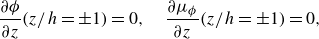 \begin{equation} \frac {\partial \phi }{\partial z}(z/h = \pm 1) = 0, \quad \frac {\partial \mu _\phi }{\partial z}(z/h = \pm 1) = 0 , \end{equation}
which are equivalent to this set of boundary conditions on the phase variable:
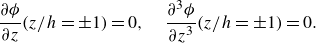 \begin{equation} \frac {\partial \phi }{\partial z}(z/h = \pm 1) = 0, \quad \frac {\partial ^3 \phi }{\partial z^3} (z/h = \pm 1) = 0 . \end{equation}
The use of these boundary conditions strictly enforces the conservation of the order parameter $\phi$
over time:
$\phi$
over time:
 \begin{equation} \frac {\partial }{\partial t}\int _\Omega \phi \, {\textrm d}\Omega = 0 , \end{equation}
where $\Omega$
is the domain considered. It is worth highlighting that the two phases are not conserved separately, but only globally. Indeed, small mass leakage between the phases may occur (Yue et al. Reference Yue, Zhou and Feng2007; Soligo et al. Reference Soligo, Roccon and Soldati2019b
; Kwakkel, Fernandino & Dorao Reference Kwakkel, Fernandino and Dorao2020). In the present simulations, this leakage – quantified as the ratio between the initial and final masses (or volumes) of the dispersed phase – is observed only during the initial stages, when an array of droplets is suddenly introduced into a turbulent flow. Specifically, the leakage amounts to approximately 10 % for
$\Omega$
is the domain considered. It is worth highlighting that the two phases are not conserved separately, but only globally. Indeed, small mass leakage between the phases may occur (Yue et al. Reference Yue, Zhou and Feng2007; Soligo et al. Reference Soligo, Roccon and Soldati2019b
; Kwakkel, Fernandino & Dorao Reference Kwakkel, Fernandino and Dorao2020). In the present simulations, this leakage – quantified as the ratio between the initial and final masses (or volumes) of the dispersed phase – is observed only during the initial stages, when an array of droplets is suddenly introduced into a turbulent flow. Specifically, the leakage amounts to approximately 10 % for $\alpha = 5.4\,\%$
, and 5 % for
$\alpha = 5.4\,\%$
, and 5 % for $\alpha = 10.6\,\%$
. After this initial transient, the mass of the dispersed phase remains constant.
$\alpha = 10.6\,\%$
. After this initial transient, the mass of the dispersed phase remains constant.
2.6. Simulation set-up
The simulations have been performed in a channel flow configuration (see figure 1) at constant friction Reynolds number $Re_\tau =300$
. The channel dimensions in outer units are
$Re_\tau =300$
. The channel dimensions in outer units are $L_x \times L_y \times L_z = 4 {\unicode[Arial]{x03C0}} h \times 2 {\unicode[Arial]{x03C0}} h \times 2h$
corresponding to
$L_x \times L_y \times L_z = 4 {\unicode[Arial]{x03C0}} h \times 2 {\unicode[Arial]{x03C0}} h \times 2h$
corresponding to $L_x^+ \times L_y^+ \times L_z^+ = 3770 \times 1885 \times 600$
wall units (w.u.). An imposed pressure gradient in the streamwise direction drives the flow. Surface tension is set via the Weber number and corresponds to that of a liquid/liquid system; the resulting Weber number is
$L_x^+ \times L_y^+ \times L_z^+ = 3770 \times 1885 \times 600$
wall units (w.u.). An imposed pressure gradient in the streamwise direction drives the flow. Surface tension is set via the Weber number and corresponds to that of a liquid/liquid system; the resulting Weber number is $We=3.0$
. The carrier phase is characterised by Prandtl number
$We=3.0$
. The carrier phase is characterised by Prandtl number $Pr_c=0.013$
, representative of liquid lead at
$Pr_c=0.013$
, representative of liquid lead at $700{-}900\ \textrm {K}$
with viscosity
$700{-}900\ \textrm {K}$
with viscosity $\mu ={1.70 \times 10^{-3}}\,\textrm {Pa s}$
, thermal conductivity
$\mu ={1.70 \times 10^{-3}}\,\textrm {Pa s}$
, thermal conductivity $\kappa _c=\textrm {18.24}\,\textrm W\, {\textrm m}^{-1}\,{{\textrm K}^{-1}}$
, and heat capacity
$\kappa _c=\textrm {18.24}\,\textrm W\, {\textrm m}^{-1}\,{{\textrm K}^{-1}}$
, and heat capacity $c_p=133.54\,{\textrm J\,{\textrm {kg}}^{-1}}\, \textrm K^{-1}$
(Fazio et al. Reference Fazio2015). For the droplets, the Prandtl number is varied within a range from
$c_p=133.54\,{\textrm J\,{\textrm {kg}}^{-1}}\, \textrm K^{-1}$
(Fazio et al. Reference Fazio2015). For the droplets, the Prandtl number is varied within a range from $Pr_d=0.013$
(same as the carrier) to
$Pr_d=0.013$
(same as the carrier) to $Pr_d=7$
(approximately 500 times larger than that of the carrier phase). To isolate the effect of thermal diffusivity on the system, we maintain a unitary density and viscosity ratio between the carrier phase and the droplets. This simplification ensures that the observed variations in heat transfer are solely due to differences in thermal diffusivity (specifically thermal conductivity), allowing for a better understanding of its influence on heat transfer.
$Pr_d=7$
(approximately 500 times larger than that of the carrier phase). To isolate the effect of thermal diffusivity on the system, we maintain a unitary density and viscosity ratio between the carrier phase and the droplets. This simplification ensures that the observed variations in heat transfer are solely due to differences in thermal diffusivity (specifically thermal conductivity), allowing for a better understanding of its influence on heat transfer.
The grid is uniform in the periodic streamwise and spanwise directions (Fourier transforms), while the Chebyshev–Gauss–Lobatto point distribution is employed in the wall-normal direction (Chebyshev polynomials). The governing equations are discretised using $N_x\times N_y\times N_z = 512\times 256\times 513$
grid points for the cases with
$N_x\times N_y\times N_z = 512\times 256\times 513$
grid points for the cases with $Pr_d\lt 1$
, while a grid
$Pr_d\lt 1$
, while a grid $N_x\times N_y\times N_z=1024\times 512\times 513$
is employed for the super-unitary droplet Prandtl number cases. Indeed, as the two phases can have different Prandtl numbers, the smallest temperature length scale – the Batchelor scale – becomes smaller as
$N_x\times N_y\times N_z=1024\times 512\times 513$
is employed for the super-unitary droplet Prandtl number cases. Indeed, as the two phases can have different Prandtl numbers, the smallest temperature length scale – the Batchelor scale – becomes smaller as $Pr_d$
is increased (Batchelor Reference Batchelor1971). Specifically, the Batchelor scale
$Pr_d$
is increased (Batchelor Reference Batchelor1971). Specifically, the Batchelor scale $\eta _\theta$
is related to the smallest flow scale – the Kolmogorov length scale
$\eta _\theta$
is related to the smallest flow scale – the Kolmogorov length scale $\eta _k$
– via the relation
$\eta _k$
– via the relation $\eta _\theta =\eta _k/\sqrt {Pr}$
. The Cahn number is set to
$\eta _\theta =\eta _k/\sqrt {Pr}$
. The Cahn number is set to $\textit {Ch}=0.02$
for all cases, and the Péclet number is set via the scaling
$\textit {Ch}=0.02$
for all cases, and the Péclet number is set via the scaling $Pe=1/\textit {Ch}=50$
(Magaletti et al. Reference Magaletti, Picano, Chinappi, Marino and Casciola2013). The chosen grid resolution and Cahn number ensure that the thermal boundary layer at the interface is always discretised with a minimum of four grid points, and that its thickness is larger than that of the thin interfacial layer. An overview of the simulation parameters is provided in table 1.
$Pe=1/\textit {Ch}=50$
(Magaletti et al. Reference Magaletti, Picano, Chinappi, Marino and Casciola2013). The chosen grid resolution and Cahn number ensure that the thermal boundary layer at the interface is always discretised with a minimum of four grid points, and that its thickness is larger than that of the thin interfacial layer. An overview of the simulation parameters is provided in table 1.
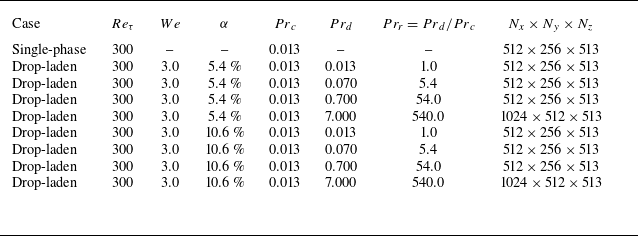
Overview of the simulation parameters. For fixed friction Reynolds number $Re_\tau =300$
and Weber number
$Re_\tau =300$
and Weber number $\textit {We}=3$
, we consider a single-phase flow case, two volume fractions and four non-isothermal drop-laden flows characterised by different dispersed phase Prandtl numbers. The grid resolution is set so as to satisfy DNS requirements.
$\textit {We}=3$
, we consider a single-phase flow case, two volume fractions and four non-isothermal drop-laden flows characterised by different dispersed phase Prandtl numbers. The grid resolution is set so as to satisfy DNS requirements.
To generate a suitable initial condition for the multiphase cases, we perform a precursor simulation of a single-phase turbulent channel flow with a linear temperature profile as an initial condition. Once the simulation reaches the steady state, we let it run for an additional $t^+=4000$
. Then we initialise
$t^+=4000$
. Then we initialise $256$
spherical droplets with diameters
$256$
spherical droplets with diameters $d=0.4h$
and
$d=0.4h$
and $d=0.5h$
corresponding to volume fractions
$d=0.5h$
corresponding to volume fractions $\alpha =5.4\,\%$
and
$\alpha =5.4\,\%$
and $10.6\,\%$
, respectively. The volume fraction is
$10.6\,\%$
, respectively. The volume fraction is $\alpha = V_d/(V_c+V_d)$
, where
$\alpha = V_d/(V_c+V_d)$
, where $V_d$
is the volume of the drops, and
$V_d$
is the volume of the drops, and $V_c$
is the volume of the carrier phase. To guarantee that the results are independent of the initial flow field condition, each case is initialised with a different realisation of the flow field. However, the fields are statistically equivalent, as they are all derived from a statistically steady turbulent channel flow.
$V_c$
is the volume of the carrier phase. To guarantee that the results are independent of the initial flow field condition, each case is initialised with a different realisation of the flow field. However, the fields are statistically equivalent, as they are all derived from a statistically steady turbulent channel flow.
3. Results
This section presents and discusses the simulation results. We begin with a qualitative analysis, followed by a characterisation of the dispersed phase topology and an examination of the temperature field in both phases. Finally, based on these findings, we introduce a phenomenological model to predict the Nusselt number as a function of the dispersed phase Prandtl number and volume fraction.
3.1. Qualitative discussion
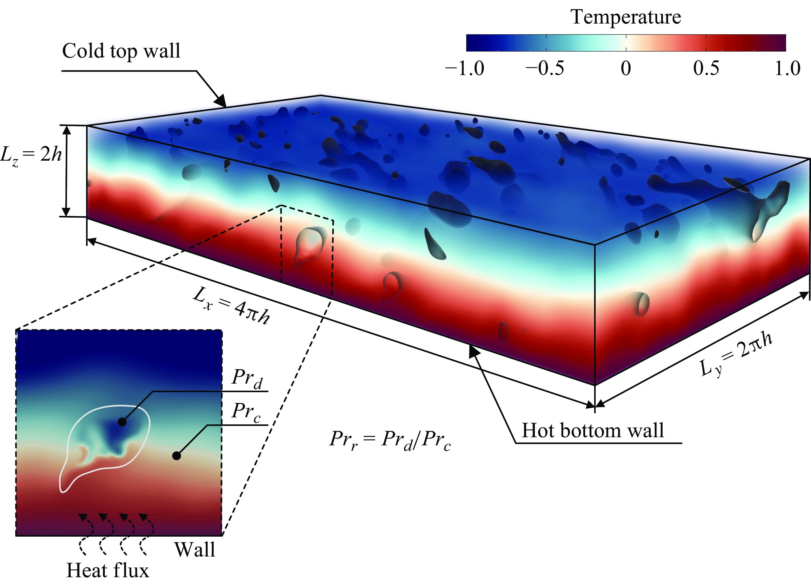
Sketch of the computational set-up employed in the present work. The flow of two immiscible phases (carrier and dispersed) between two differentially heated walls is considered. The bottom wall has a constant high temperature, while the top wall is cold. The carrier flow is characterised by a low Prandtl number $Pr_c=0.013$
, while different values of the dispersed phase Prandtl number have been considered, from
$Pr_c=0.013$
, while different values of the dispersed phase Prandtl number have been considered, from $Pr_d=0.013$
up to
$Pr_d=0.013$
up to $Pr_d=7$
. The close-up view shows the temperature field in a plane crossing one droplet, and refers to
$Pr_d=7$
. The close-up view shows the temperature field in a plane crossing one droplet, and refers to $Pr_d/Pr_c=540$
, thus
$Pr_d/Pr_c=540$
, thus $Pr_d=7.0$
.
$Pr_d=7.0$
.
At the beginning of the simulations $(t^+=0)$
, droplets are injected into the turbulent flow. Immediately, turbulence starts to deform the interface of the droplets (Lu & Tryggvason Reference Lu and Tryggvason2018; Soligo et al. Reference Soligo, Roccon and Soldati2019a
; Cannon, Soligo & Rosti Reference Cannon, Soligo and Rosti2024; Crialesi-Esposito et al. Reference Crialesi-Esposito, Boffetta, Brandt, Chibbaro and Musacchio2024). The interaction between the turbulent eddies and the droplets leads to coalescence and breakage events, which continue dynamically throughout the simulation. After an initial transient phase, a statistical equilibrium is reached, wherein the rate of droplet breakage balances out with the coalescence events. This equilibrium determines the average droplet count, and results in a statistically steady droplet size distribution (DSD). Simultaneously, the temperature field is significantly altered by the presence of the droplets, which not only disrupt the turbulent structures but are also characterised by different thermal properties (
$(t^+=0)$
, droplets are injected into the turbulent flow. Immediately, turbulence starts to deform the interface of the droplets (Lu & Tryggvason Reference Lu and Tryggvason2018; Soligo et al. Reference Soligo, Roccon and Soldati2019a
; Cannon, Soligo & Rosti Reference Cannon, Soligo and Rosti2024; Crialesi-Esposito et al. Reference Crialesi-Esposito, Boffetta, Brandt, Chibbaro and Musacchio2024). The interaction between the turbulent eddies and the droplets leads to coalescence and breakage events, which continue dynamically throughout the simulation. After an initial transient phase, a statistical equilibrium is reached, wherein the rate of droplet breakage balances out with the coalescence events. This equilibrium determines the average droplet count, and results in a statistically steady droplet size distribution (DSD). Simultaneously, the temperature field is significantly altered by the presence of the droplets, which not only disrupt the turbulent structures but are also characterised by different thermal properties ( $Pr_r\neq 1$
) with respect to the carrier phase. These differences result in distinct heat conduction behaviours inside and outside the droplets. This complex dynamic is represented in figure 1: the droplets are identified by the iso-contour
$Pr_r\neq 1$
) with respect to the carrier phase. These differences result in distinct heat conduction behaviours inside and outside the droplets. This complex dynamic is represented in figure 1: the droplets are identified by the iso-contour $\phi =0$
, while the volume rendering shows the temperature distribution in the domain. The close-up view highlights the temperature modifications inside and in the proximity of a droplet, which is characterised by a different Prandtl number (the case shown refers to
$\phi =0$
, while the volume rendering shows the temperature distribution in the domain. The close-up view highlights the temperature modifications inside and in the proximity of a droplet, which is characterised by a different Prandtl number (the case shown refers to $Pr_r=540$
, corresponding to
$Pr_r=540$
, corresponding to $Pr_d=7$
). Within the droplets, the temperature field exhibits noticeable fluctuations, whereas in the carrier phase, it follows an approximately linear profile from top to bottom. Regarding the dispersed phase, although the imposed pressure gradient establishes a primary flow direction, the turbulent shear stresses induce local velocity fluctuations in all three components. As a result, the drops experience secondary motions in the spanwise and wall-normal directions. In particular, the wall-normal fluctuations advect the droplets from the bottom (hot) to the top (cold) region of the channel, and vice versa.
$Pr_d=7$
). Within the droplets, the temperature field exhibits noticeable fluctuations, whereas in the carrier phase, it follows an approximately linear profile from top to bottom. Regarding the dispersed phase, although the imposed pressure gradient establishes a primary flow direction, the turbulent shear stresses induce local velocity fluctuations in all three components. As a result, the drops experience secondary motions in the spanwise and wall-normal directions. In particular, the wall-normal fluctuations advect the droplets from the bottom (hot) to the top (cold) region of the channel, and vice versa.
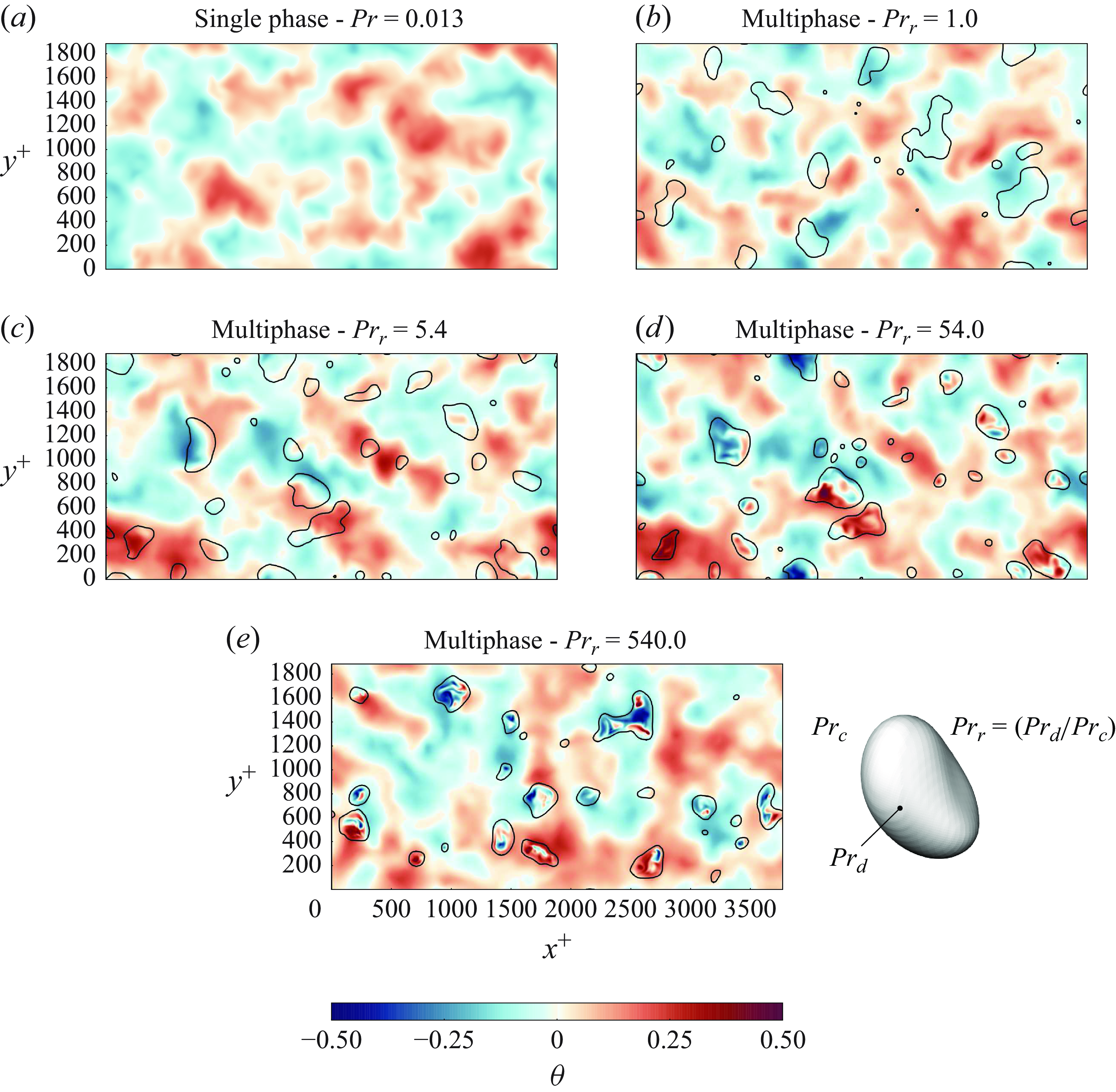
Instantaneous top-down views of the temperature fields $\theta$
in the wall-normal direction (
$\theta$
in the wall-normal direction ( $z=0$
) at statistically steady state
$z=0$
) at statistically steady state $(t^+=2505)$
. Black solid lines indicate droplet interfaces (
$(t^+=2505)$
. Black solid lines indicate droplet interfaces ( $\phi =0$
), with flow direction from left to right. Increasing the Prandtl ratio
$\phi =0$
), with flow direction from left to right. Increasing the Prandtl ratio $Pr_r$
enhances temperature modifications both within the droplets and in the carrier. Here, the volume fraction is
$Pr_r$
enhances temperature modifications both within the droplets and in the carrier. Here, the volume fraction is $\alpha =5.4\,\%$
.
$\alpha =5.4\,\%$
.
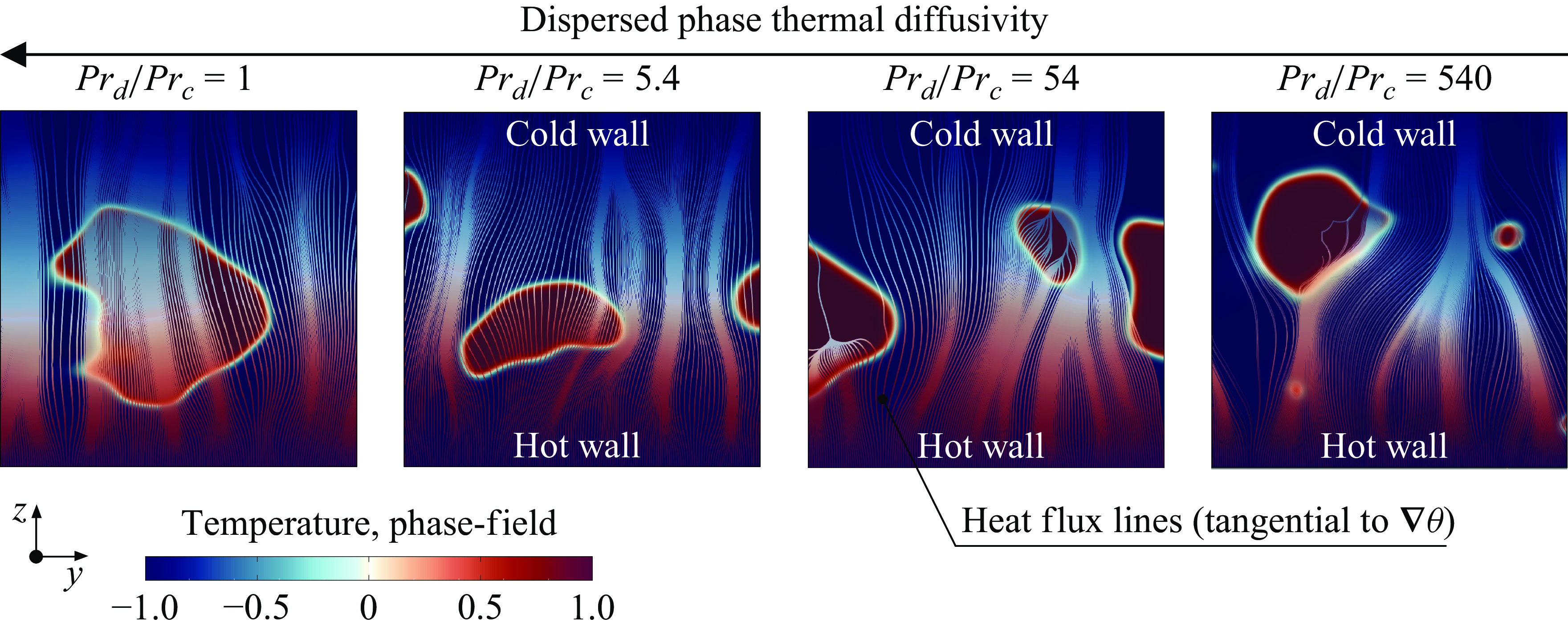
Phase-field variable (blue for carrier, red for droplets) and heat-flux lines (tangential to $\boldsymbol{\nabla} \theta$
) coloured according to the local temperature (blue for cold, red for hot) in a subsection of a
$\boldsymbol{\nabla} \theta$
) coloured according to the local temperature (blue for cold, red for hot) in a subsection of a $y{-}z$
plane. The Prandtl number of the carrier phase is fixed, and moving from left to right, the droplet Prandtl number increases. As
$y{-}z$
plane. The Prandtl number of the carrier phase is fixed, and moving from left to right, the droplet Prandtl number increases. As $Pr_d/Pr_c$
is increased (via a reduction of the dispersed phase thermal diffusivity), convective phenomena become more important inside the droplets, and the dissipation takes place at smaller scales, increasing the thermal inertia. As a consequence, the heat flux is deflected, favouring pathways with higher thermal conductivity. It is worth noting that smaller droplets offer lower thermal resistance since they experience less intense temperature gradients.
$Pr_d/Pr_c$
is increased (via a reduction of the dispersed phase thermal diffusivity), convective phenomena become more important inside the droplets, and the dissipation takes place at smaller scales, increasing the thermal inertia. As a consequence, the heat flux is deflected, favouring pathways with higher thermal conductivity. It is worth noting that smaller droplets offer lower thermal resistance since they experience less intense temperature gradients.
From the Prandtl number definition, we know that the thermal diffusivity decreases for increasing values of $Pr$
as the viscosity in the system is uniform. This decreased thermal diffusivity implies that drops characterised by a larger
$Pr$
as the viscosity in the system is uniform. This decreased thermal diffusivity implies that drops characterised by a larger $Pr_d$
(i.e. larger
$Pr_d$
(i.e. larger $Pr_r$
) would need more time to relax to the thermal equilibrium with their surroundings. Consequently, when advected by the turbulent flow, these droplets cannot immediately adjust their temperature to match the local temperature of the carrier fluid. With these theoretical insights in mind, we analyse figure 2, which presents the temperature distribution in a slice parallel to the wall at the centre of the channel (
$Pr_r$
) would need more time to relax to the thermal equilibrium with their surroundings. Consequently, when advected by the turbulent flow, these droplets cannot immediately adjust their temperature to match the local temperature of the carrier fluid. With these theoretical insights in mind, we analyse figure 2, which presents the temperature distribution in a slice parallel to the wall at the centre of the channel ( $z=0$
) for different cases with volume fraction
$z=0$
) for different cases with volume fraction $\alpha =5.4\,\%$
. First, we consider the single-phase reference case (figure 2
$\alpha =5.4\,\%$
. First, we consider the single-phase reference case (figure 2 $a$
) where only one phase is present (
$a$
) where only one phase is present ( $Pr_c=0.013$
). The turbulent flow generates temperature fluctuations, though they remain small, approximately
$Pr_c=0.013$
). The turbulent flow generates temperature fluctuations, though they remain small, approximately $2\,\%$
of the imposed temperature difference. Moving to the drop-laden cases, we first consider the scenario where the carrier and dispersed phases share the same thermophysical properties (
$2\,\%$
of the imposed temperature difference. Moving to the drop-laden cases, we first consider the scenario where the carrier and dispersed phases share the same thermophysical properties ( $Pr_d=Pr_c=0.013$
, figure 2
$Pr_d=Pr_c=0.013$
, figure 2 $b$
). Here, the temperature field remains similar to the single-phase case as the larger thermal diffusivity allows the drops to adjust their internal temperature to that of the carrier fluid. In contrast, when the drops have a higher Prandtl number than the carrier phase (
$b$
). Here, the temperature field remains similar to the single-phase case as the larger thermal diffusivity allows the drops to adjust their internal temperature to that of the carrier fluid. In contrast, when the drops have a higher Prandtl number than the carrier phase ( $Pr_r \gt 1$
, figure 2
$Pr_r \gt 1$
, figure 2 $c$
–
$c$
– $e$
), the temperature distribution becomes more irregular, with distinct hot and cold spots. As
$e$
), the temperature distribution becomes more irregular, with distinct hot and cold spots. As $Pr_r$
increases from
$Pr_r$
increases from $Pr_r=5.4$
to
$Pr_r=5.4$
to $Pr_r=540$
, temperature fluctuations intensify, and complex temperature patterns emerge. The characteristic temperature length scales also become smaller, as expected from theoretical arguments (Batchelor Reference Batchelor1971). Notably, the increased Prandtl number of the dispersed phase also influences the carrier fluid, leading to a slight amplification of temperature fluctuations, as evident from the red and blue regions. These modifications can be better appreciated by considering a cross-section of the channel. Figure 3 shows the heat-flux lines in a
$Pr_r=540$
, temperature fluctuations intensify, and complex temperature patterns emerge. The characteristic temperature length scales also become smaller, as expected from theoretical arguments (Batchelor Reference Batchelor1971). Notably, the increased Prandtl number of the dispersed phase also influences the carrier fluid, leading to a slight amplification of temperature fluctuations, as evident from the red and blue regions. These modifications can be better appreciated by considering a cross-section of the channel. Figure 3 shows the heat-flux lines in a $y$
–
$y$
– $z$
plane for different
$z$
plane for different $Pr_r$
. Heat-flux lines are tangent to the temperature gradient and thus perpendicular to the iso-temperature contours. The background depicts the phase topology, with drops in red and carrier phase in blue, while the heat-flux lines are colour-coded according to the local temperature, transitioning from red (hot bottom wall) to blue (cold top wall). As
$Pr_r$
. Heat-flux lines are tangent to the temperature gradient and thus perpendicular to the iso-temperature contours. The background depicts the phase topology, with drops in red and carrier phase in blue, while the heat-flux lines are colour-coded according to the local temperature, transitioning from red (hot bottom wall) to blue (cold top wall). As $Pr_d$
increases, the heat-flux lines become increasingly deflected by the drops, eventually bypassing the dispersed phase entirely (
$Pr_d$
increases, the heat-flux lines become increasingly deflected by the drops, eventually bypassing the dispersed phase entirely ( $Pr_r = 540$
, rightmost panel). This effect arises from the enhanced thermal inertia and reduced conductivity of the drops when
$Pr_r = 540$
, rightmost panel). This effect arises from the enhanced thermal inertia and reduced conductivity of the drops when $Pr_r$
is studied. A similar trend has been observed in other flow configurations involving larger conductivity differences between the two phases, e.g. melting problems (Shangguan, Ahuja & Stefanescu Reference Shangguan, Ahuja and Stefanescu1992; van Buuren et al. Reference van Buuren, Kant, Meijer, Diddens and Lohse2024). These initial observations suggest that drops create a series of gaps in the path of heat from the hot bottom wall to the cold top wall, thus reducing the area available for the heat exchange.
$Pr_r$
is studied. A similar trend has been observed in other flow configurations involving larger conductivity differences between the two phases, e.g. melting problems (Shangguan, Ahuja & Stefanescu Reference Shangguan, Ahuja and Stefanescu1992; van Buuren et al. Reference van Buuren, Kant, Meijer, Diddens and Lohse2024). These initial observations suggest that drops create a series of gaps in the path of heat from the hot bottom wall to the cold top wall, thus reducing the area available for the heat exchange.
3.2. Dispersed phase topology
We start to quantify these observations by characterising the dispersed phase topology. To this aim, we consider the DSD obtained at steady state. The DSD is an important result for the modelling of multiphase flows and will be useful in the final part of the paper where the heat transfer performance will be modelled. Indeed, once the distribution is known, important parameters such as the amount of interfacial area, which has an important role in heat and transfer problems, can be evaluated. The most important length scale to analyse the DSD is the Kolmogorov–Hinze diameter (Hinze Reference Hinze1955; Kolmogorov Reference Kolmogorov1991). This scale represents the maximum stable diameter for a non-breaking droplet. This diameter can be calculated from the balance between the destabilising forces that act on the droplet surface (e.g. turbulence-induced stresses) and the stabilising action of surface tension forces, which try to minimise the droplet surface and restore the spherical shape, thus avoiding droplet breakage. For the present configuration (turbulent channel flow), this diameter can be estimated as (Soligo et al. Reference Soligo, Roccon and Soldati2019a )
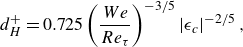 \begin{equation} d_H^+ = 0.725\left (\frac {We}{Re_{\tau }}\right )^{-3/5} \left |\epsilon _c\right |^{-2/5}, \end{equation}
where $\epsilon _c$
is the turbulent dissipation evaluated at the channel centre, where droplets preferentially accumulate. For a fixed Reynolds number, higher Weber numbers correspond to weaker surface tension forces, leading to smaller maximum stable droplet diameters.
$\epsilon _c$
is the turbulent dissipation evaluated at the channel centre, where droplets preferentially accumulate. For a fixed Reynolds number, higher Weber numbers correspond to weaker surface tension forces, leading to smaller maximum stable droplet diameters.
Probability density function of droplet equivalent diameter $d^+_{eq}$
normalised by the Kolmogorov–Hinze scale. Results at low volume fraction (
$d^+_{eq}$
normalised by the Kolmogorov–Hinze scale. Results at low volume fraction ( $\alpha =5.4\,\%$
) are reported with empty symbols, while those at high volume fraction (
$\alpha =5.4\,\%$
) are reported with empty symbols, while those at high volume fraction ( $\alpha =10.6\,\%$
) are reported with full symbols. The analytic scaling laws for the coalescence- and breakage-dominated regimes,
$\alpha =10.6\,\%$
) are reported with full symbols. The analytic scaling laws for the coalescence- and breakage-dominated regimes, ${d^+}^{-3/2}$
and
${d^+}^{-3/2}$
and ${d^+}^{-10/3}$
, are also reported for reference. Good agreement is obtained in the breakage-dominated regime (drops larger than the Kolmogorov–Hinze scale).
${d^+}^{-10/3}$
, are also reported for reference. Good agreement is obtained in the breakage-dominated regime (drops larger than the Kolmogorov–Hinze scale).

Figure 4 shows the distributions obtained from the different cases. The DSDs have been computed from $t^+=1000$
up to
$t^+=1000$
up to $t^+=4500$
. Results at low volume fraction (
$t^+=4500$
. Results at low volume fraction ( $\alpha =5.4\,\%$
) are reported with empty symbols, while those at high volume fraction (
$\alpha =5.4\,\%$
) are reported with empty symbols, while those at high volume fraction ( $\alpha =10.6\,\%$
) are reported with full symbols. The simulated cases are reported using different colours:
$\alpha =10.6\,\%$
) are reported with full symbols. The simulated cases are reported using different colours: $Pr_r=1$
dark violet,
$Pr_r=1$
dark violet, $Pr_r=5.4$
violet,
$Pr_r=5.4$
violet, $Pr_r=54.0$
light violet, and
$Pr_r=54.0$
light violet, and $Pr_r=540.0$
orange. The analytic scaling laws for the coalescence- and breakage-dominated regimes,
$Pr_r=540.0$
orange. The analytic scaling laws for the coalescence- and breakage-dominated regimes, ${d^+}^{-3/2}$
and
${d^+}^{-3/2}$
and ${d^+}^{-10/3}$
, are also reported for reference (Garrett, Li & Farmer Reference Garrett, Li and Farmer2000). Diameters are reported normalised by the Kolmogorov–Hinze scale, which for
${d^+}^{-10/3}$
, are also reported for reference (Garrett, Li & Farmer Reference Garrett, Li and Farmer2000). Diameters are reported normalised by the Kolmogorov–Hinze scale, which for $We=3.0$
and
$We=3.0$
and $Re_\tau =300$
is
$Re_\tau =300$
is $d^+_H\approx 125\ \text{w.u.}$
Present results are also compared with archival literature data on DSD obtained in previous works that investigated the breakage of drops/bubbles in turbulent flows. In particular, the following results are reported: breakage of surfactant-laden drop in homogeneous isotropic turbulence (Mukherjee et al. Reference Mukherjee, Safdari, Shardt, Kenjereš and Van den Akker2019; Cannon et al. Reference Cannon, Soligo and Rosti2024), breakage of surfactant-laden drop in turbulent channel flow (Soligo et al. Reference Soligo, Roccon and Soldati2019a
), and breakage of clean drops in homogeneous isotropic turbulence (Crialesi-Esposito, Chibbaro & Brandt Reference Crialesi-Esposito, Chibbaro and Brandt2023).
$d^+_H\approx 125\ \text{w.u.}$
Present results are also compared with archival literature data on DSD obtained in previous works that investigated the breakage of drops/bubbles in turbulent flows. In particular, the following results are reported: breakage of surfactant-laden drop in homogeneous isotropic turbulence (Mukherjee et al. Reference Mukherjee, Safdari, Shardt, Kenjereš and Van den Akker2019; Cannon et al. Reference Cannon, Soligo and Rosti2024), breakage of surfactant-laden drop in turbulent channel flow (Soligo et al. Reference Soligo, Roccon and Soldati2019a
), and breakage of clean drops in homogeneous isotropic turbulence (Crialesi-Esposito, Chibbaro & Brandt Reference Crialesi-Esposito, Chibbaro and Brandt2023).
By analysing figure 4, it is possible to identify two distinct regimes based on droplet diameter. For droplets smaller than the Kolmogorov–Hinze scale, a coalescence-dominated regime is observed. In this regime, drop breakage is unlikely, as the droplets remain below the critical scale. Instead, they primarily grow by coalescing with other drops. For droplets larger than the Kolmogorov–Hinze scale, a breakage-dominated regime emerges, where droplet size changes predominantly through breakage. Across all simulated cases, the results align with the expected scaling law in this regime. In the coalescence regime, identifying a clear trend is challenging. However, satisfactory agreement is observed for droplets exceeding 50 w.u., corresponding to $d^+_{eq}/d^+_{H} \gt 0.4$
. The dispersed phase Prandtl number does not influence the DSD, as temperature acts as a passive scalar. Conversely, volume fraction affects the distribution: for
$d^+_{eq}/d^+_{H} \gt 0.4$
. The dispersed phase Prandtl number does not influence the DSD, as temperature acts as a passive scalar. Conversely, volume fraction affects the distribution: for $\alpha = 10.6\,\%$
, there is a slightly higher probability of smaller drops compared to
$\alpha = 10.6\,\%$
, there is a slightly higher probability of smaller drops compared to $\alpha = 5.4\,\%$
. Additionally, the solid markers (
$\alpha = 5.4\,\%$
. Additionally, the solid markers ( $\alpha = 10.6\,\%$
) on the right-hand side of figure 4 span a broader diameter range, indicating the presence of larger droplets within the channel.
$\alpha = 10.6\,\%$
) on the right-hand side of figure 4 span a broader diameter range, indicating the presence of larger droplets within the channel.
3.3. Characterisation of the temperature field
The presence of a swarm of large and deformable droplets has a negligible effect on macroscopic flow parameters such as the flow rate and required pressure gradient (Cannon et al. Reference Cannon, Izbassarov, Tammisola, Brandt and Rosti2021; Mangani et al. Reference Mangani, Soligo, Roccon and Soldati2022). For this reason, we focus on the characterisation of the temperature field and heat transfer performance of the multiphase system. All the statistics presented in the following are computed when the system reaches the new steady-state configuration in terms of heat transfer and dispersed phase topology. To verify that the simulations have reached this condition, we analyse the time evolution of the Nusselt number defined as the dimensionless heat flux at the walls:
 \begin{equation} \textit {Nu}=\frac {2q_w h}{\kappa _c\Delta \theta }\, , \end{equation}
where $q_w$
is the heat flux evaluated at the wall,
$q_w$
is the heat flux evaluated at the wall, $\kappa_c$
, is the carrier phase thermal conductivity,
$\kappa_c$
, is the carrier phase thermal conductivity, $\Delta \theta$
is the temperature difference between the two walls, and
$\Delta \theta$
is the temperature difference between the two walls, and $h$
is the half-height of the channel.
$h$
is the half-height of the channel.
Temporal evolution of the Nusselt number $\textit {Nu}$
averaged between the two walls and normalised by the single-phase value
$\textit {Nu}$
averaged between the two walls and normalised by the single-phase value $Nu_s$
: (a)
$Nu_s$
: (a) $\alpha =5.4\,\%$
, and (b)
$\alpha =5.4\,\%$
, and (b) $\alpha =10.6\,\%$
. The grey box highlights the transient required before the simulations reach the new steady-state configuration.
$\alpha =10.6\,\%$
. The grey box highlights the transient required before the simulations reach the new steady-state configuration.
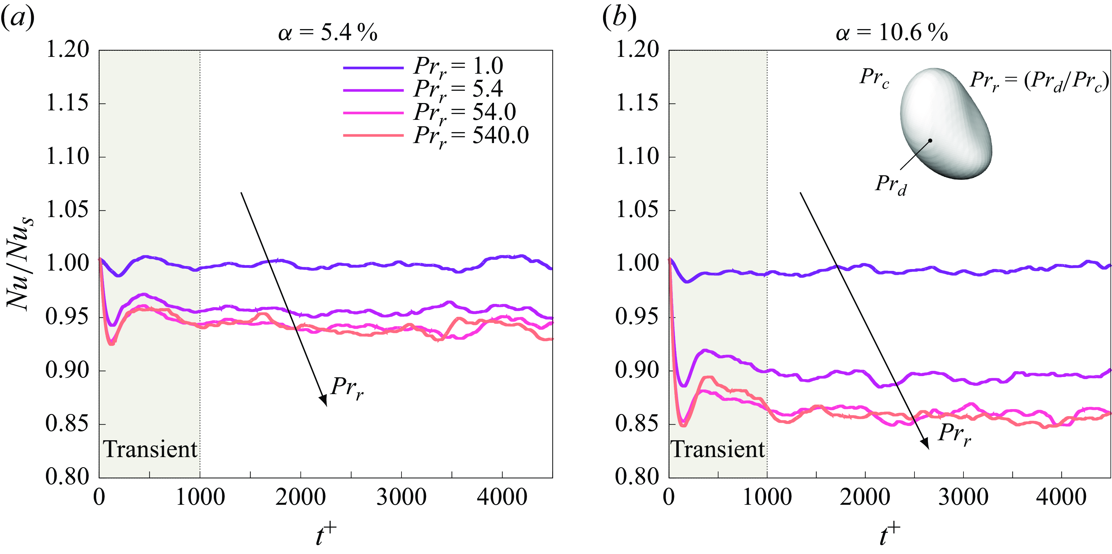
The time evolution of the Nusselt number is shown in figure 5. The different cases are reported using different colours: $Pr_r=1$
dark violet,
$Pr_r=1$
dark violet, ${Pr}_r=5.4$
violet,
${Pr}_r=5.4$
violet, ${Pr}_r=54.0$
light violet, and
${Pr}_r=54.0$
light violet, and ${Pr}_r=540$
orange. The results are shown normalised by the single-phase value (
${Pr}_r=540$
orange. The results are shown normalised by the single-phase value ( $\textit {Nu}_s \approx 1.1$
). We observe that after approximately
$\textit {Nu}_s \approx 1.1$
). We observe that after approximately $t^+=1000$
, a steady-state condition is achieved for both volume fractions. This observation aligns with the previous finding of Mangani et al. (Reference Mangani, Soligo, Roccon and Soldati2022), who showed that for the same set of parameters considered in this study (Reynolds and Weber numbers), the rates of breakage and coalescence converge to a statistical equilibrium. Consequently, once the droplets reach a dynamic steady state, the average heat flux at the wall also stabilises. When examining the steady-state values for each case, we note that increasing the Prandtl number ratio (i.e. the dispersed phase Prandtl number) leads to a decrease in both the Nusselt number and the corresponding heat transfer at the wall. This trend is more pronounced for the higher volume fractions, where the Nusselt number decreases by nearly 15 % for the higher
$t^+=1000$
, a steady-state condition is achieved for both volume fractions. This observation aligns with the previous finding of Mangani et al. (Reference Mangani, Soligo, Roccon and Soldati2022), who showed that for the same set of parameters considered in this study (Reynolds and Weber numbers), the rates of breakage and coalescence converge to a statistical equilibrium. Consequently, once the droplets reach a dynamic steady state, the average heat flux at the wall also stabilises. When examining the steady-state values for each case, we note that increasing the Prandtl number ratio (i.e. the dispersed phase Prandtl number) leads to a decrease in both the Nusselt number and the corresponding heat transfer at the wall. This trend is more pronounced for the higher volume fractions, where the Nusselt number decreases by nearly 15 % for the higher ${Pr}_r$
.
${Pr}_r$
.
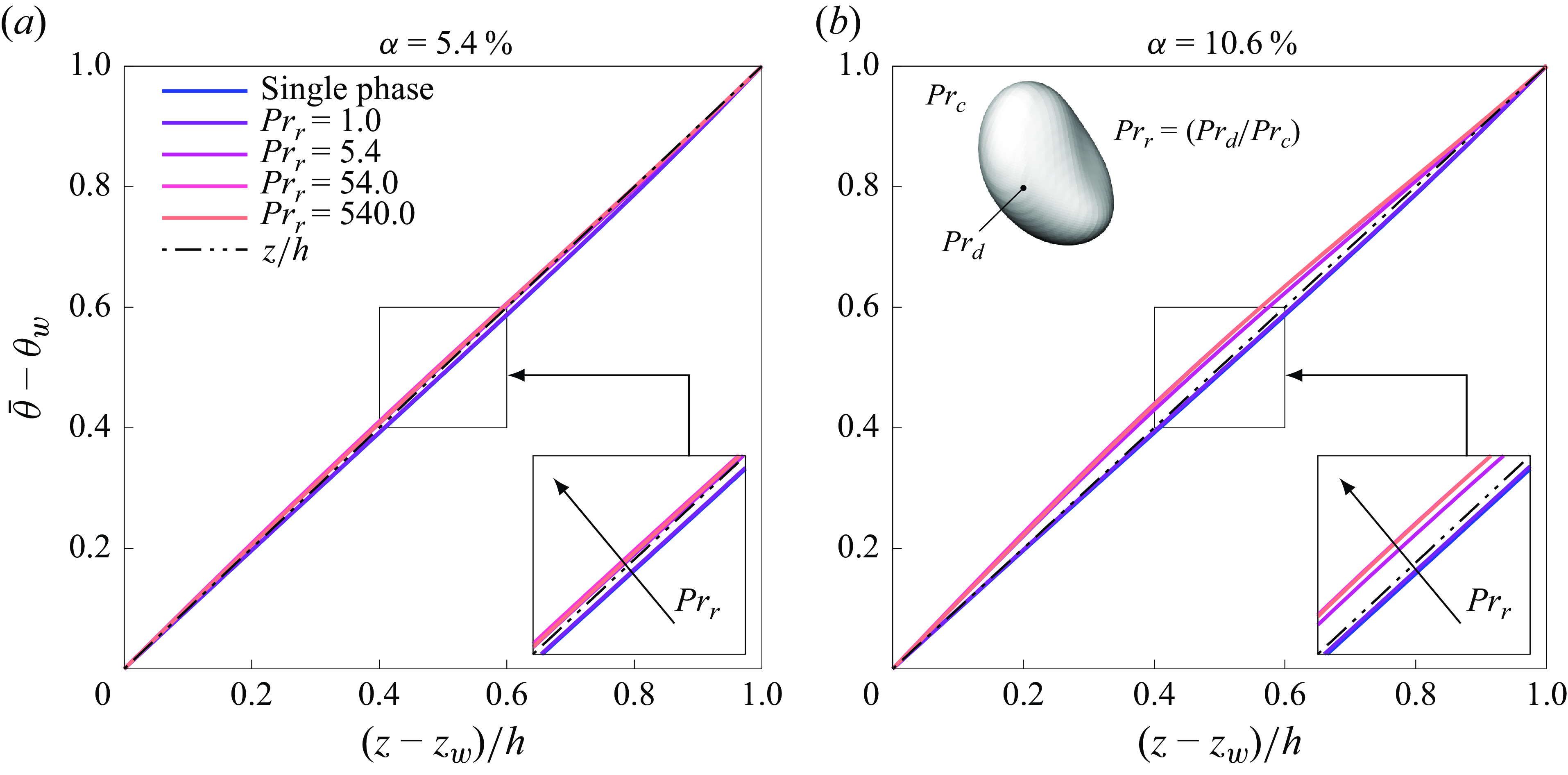
To obtain further insights into the modifications on the temperature field induced by varying the Prandtl number of the dispersed phase, we consider the behaviour of temperature statistics along the wall-normal direction. Figure 6 shows the mean temperature profiles, averaged in time and along the two homogeneous directions (x and y). The temperature expressed in outer units, denoted by the superscript $-$
, is defined as
$-$
, is defined as
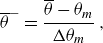 \begin{equation} \overline {\theta }^-=\frac {\overline {\theta }-\theta _m}{\Delta \theta _m}\, , \end{equation}
where the overline $\overline {(\cdot )}$
represents the averaging operator,
$\overline {(\cdot )}$
represents the averaging operator, $\theta _m=(\theta _H+\theta _C)/2$
is the mean temperature at channel centre, and
$\theta _m=(\theta _H+\theta _C)/2$
is the mean temperature at channel centre, and $\Delta \theta _m=(\theta _H-\theta _C)/2$
is the temperature difference between the two walls.
$\Delta \theta _m=(\theta _H-\theta _C)/2$
is the temperature difference between the two walls.
Mean temperature profiles in the wall-normal direction, for volume fractions (a) $\alpha =5.4\,\%$
and (b)
$\alpha =5.4\,\%$
and (b) $\alpha =10.6\,\%$
. The black dash-dotted line represents the linear law of the thermal diffusive sublayer. The insets highlight the differences among the different cases.
$\alpha =10.6\,\%$
. The black dash-dotted line represents the linear law of the thermal diffusive sublayer. The insets highlight the differences among the different cases.
Considering that $\theta _m=0$
and
$\theta _m=0$
and $\Delta \theta _m=1$
, hereafter we drop the superscript
$\Delta \theta _m=1$
, hereafter we drop the superscript $-$
, implying that all quantities are expressed in outer units unless stated otherwise. The statistics are presented as functions of the distance from the wall
$-$
, implying that all quantities are expressed in outer units unless stated otherwise. The statistics are presented as functions of the distance from the wall $z-z_w$
made dimensionless by the channel half-width
$z-z_w$
made dimensionless by the channel half-width $h$
; only half of the channel height is reported, as statistics are symmetrised. For a laminar flow, the temperature profile would exhibit a perfectly linear trend, as only diffusive and streamwise convective contributions are present. Therefore, heat transfer between the walls is purely governed by conduction in the absence of turbulence. The laminar profile is shown in figure 6 using a black dash-dotted line as a reference. In turbulent conditions, the temperature profile retains a laminar-like behaviour for low-Prandtl-number flows, as demonstrated in previous studies (Kasagi et al. Reference Kasagi, Tomita and Kuroda1993; Kawamura et al. Reference Kawamura, Ohsaka, Abe and Yamamoto1998, Reference Kawamura, Abe and Matsuo1999; Pirozzoli Reference Pirozzoli2023). Following the procedure of Piller et al. (Reference Piller, Nobile and Hanratty2002), we found that the ratio between molecular and turbulent diffusivity is approximately
$h$
; only half of the channel height is reported, as statistics are symmetrised. For a laminar flow, the temperature profile would exhibit a perfectly linear trend, as only diffusive and streamwise convective contributions are present. Therefore, heat transfer between the walls is purely governed by conduction in the absence of turbulence. The laminar profile is shown in figure 6 using a black dash-dotted line as a reference. In turbulent conditions, the temperature profile retains a laminar-like behaviour for low-Prandtl-number flows, as demonstrated in previous studies (Kasagi et al. Reference Kasagi, Tomita and Kuroda1993; Kawamura et al. Reference Kawamura, Ohsaka, Abe and Yamamoto1998, Reference Kawamura, Abe and Matsuo1999; Pirozzoli Reference Pirozzoli2023). Following the procedure of Piller et al. (Reference Piller, Nobile and Hanratty2002), we found that the ratio between molecular and turbulent diffusivity is approximately $8.5$
at the centre of the channel. This indicates that turbulent mixing is less effective in redistributing temperature compared to momentum, leading to an extended conductive sublayer that spans the entire channel width. The presence of drops slightly modifies the mean temperature profiles despite remaining approximately linear. The main effect is visible at
$8.5$
at the centre of the channel. This indicates that turbulent mixing is less effective in redistributing temperature compared to momentum, leading to an extended conductive sublayer that spans the entire channel width. The presence of drops slightly modifies the mean temperature profiles despite remaining approximately linear. The main effect is visible at $z/h=0.5$
, where the difference with the single-phase case is approximately
$z/h=0.5$
, where the difference with the single-phase case is approximately $5\,\%$
for the lower volume fraction case, and approximately
$5\,\%$
for the lower volume fraction case, and approximately $11\,\%$
for the high volume fraction case. From the inset of figure 6(
$11\,\%$
for the high volume fraction case. From the inset of figure 6( $a$
), we can see that the mean temperature profiles of
$a$
), we can see that the mean temperature profiles of ${Pr}_r=5.4,54, 540$
are almost superposed on each other. On the other hand, the inset of figure 6(
${Pr}_r=5.4,54, 540$
are almost superposed on each other. On the other hand, the inset of figure 6( $b$
) shows that the effect of
$b$
) shows that the effect of ${Pr}_r$
is more important, and that only the profiles of
${Pr}_r$
is more important, and that only the profiles of ${Pr}_r=54$
and
${Pr}_r=54$
and $540$
are superposed. This suggests that there is a saturation in the effect of
$540$
are superposed. This suggests that there is a saturation in the effect of ${Pr}_r$
, and that this effect also depends on the volume fraction.
${Pr}_r$
, and that this effect also depends on the volume fraction.
The RMS of the temperature at different ${Pr}_r$
as a function of the wall-normal distance in outer units: (
${Pr}_r$
as a function of the wall-normal distance in outer units: ( $a$
) lower volume fraction considered (
$a$
) lower volume fraction considered ( $\alpha =5.4\,\%$
), (
$\alpha =5.4\,\%$
), ( $b$
) larger volume fraction (
$b$
) larger volume fraction ( $ \alpha =10.6\,\%$
).
$ \alpha =10.6\,\%$
).
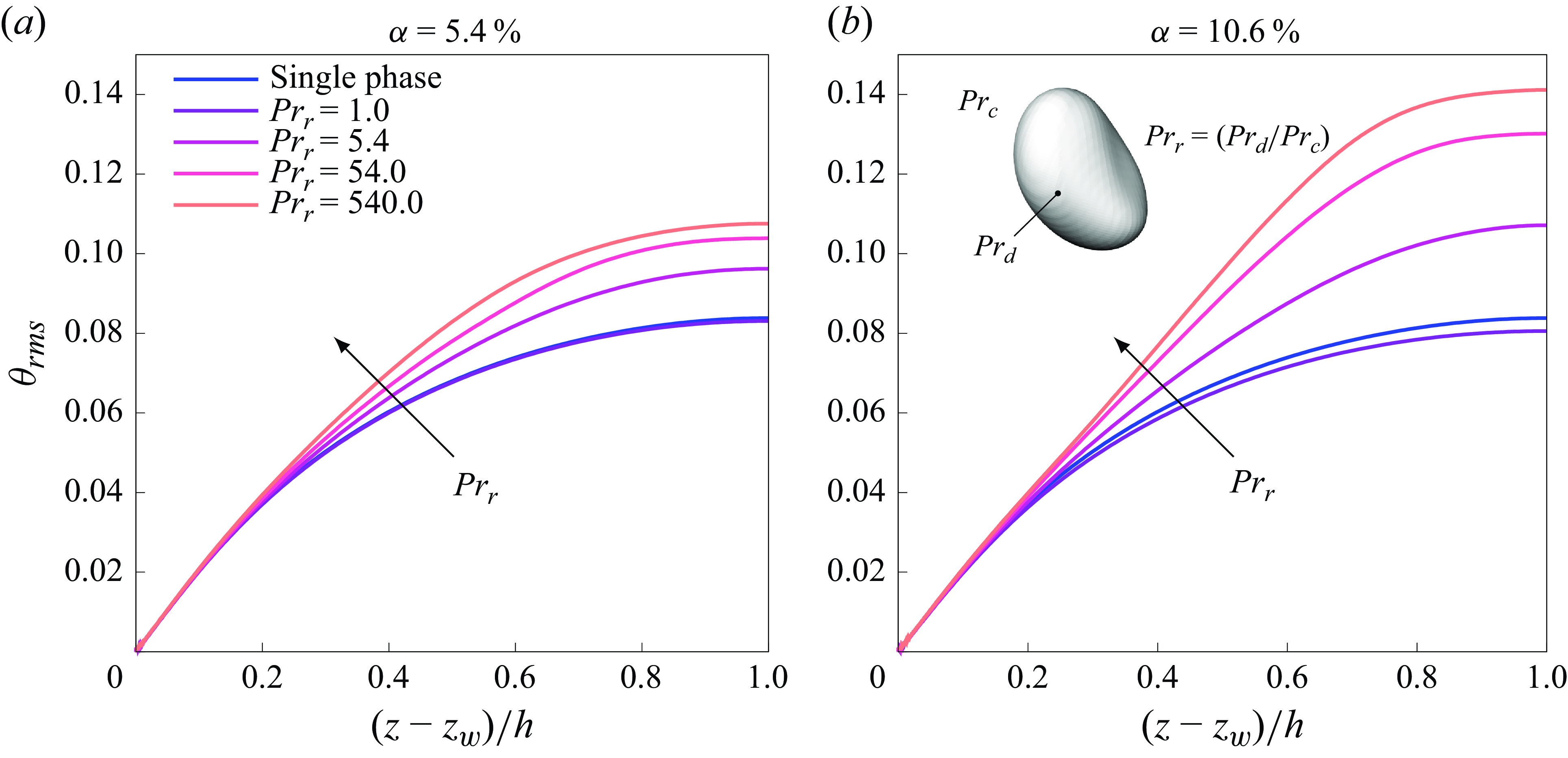
We now analyse the effect of the dispersed phase Prandtl number on higher-order statistics. Figure 7 shows the root mean square (RMS) of the temperature as a function of the wall-normal distance for $\alpha =5.4\,\%$
(figure 7
a) and
$\alpha =5.4\,\%$
(figure 7
a) and $\alpha =10.6\,\%$
(figure 7
b). Here, results are obtained by averaging temperature in both phases. The RMS exhibits a monotonic trend: starting from zero at the wall, it increases and peaks at the channel centre. This behaviour is driven by the production term (proportional to the mean temperature gradient), which remains non-zero at the channel centre (Kawamura, Abe & Shingai Reference Kawamura, Abe and Shingai2000). The presence of drops enhances the peak value attained at the channel centre, depending on both
$\alpha =10.6\,\%$
(figure 7
b). Here, results are obtained by averaging temperature in both phases. The RMS exhibits a monotonic trend: starting from zero at the wall, it increases and peaks at the channel centre. This behaviour is driven by the production term (proportional to the mean temperature gradient), which remains non-zero at the channel centre (Kawamura, Abe & Shingai Reference Kawamura, Abe and Shingai2000). The presence of drops enhances the peak value attained at the channel centre, depending on both ${Pr}_r$
and the volume fraction. An increase of the dispersed phase Prandtl number (i.e. a decrease in thermal conductivity) does not significantly influence the temperature RMS as the mean temperature profile is only slightly modified (and thus the production term). However, the dissipation reduces within the dispersed phase (Piller et al. Reference Piller, Nobile and Hanratty2002), leading to an overall increase in the RMS. The volume fraction further amplifies the effect of
${Pr}_r$
and the volume fraction. An increase of the dispersed phase Prandtl number (i.e. a decrease in thermal conductivity) does not significantly influence the temperature RMS as the mean temperature profile is only slightly modified (and thus the production term). However, the dissipation reduces within the dispersed phase (Piller et al. Reference Piller, Nobile and Hanratty2002), leading to an overall increase in the RMS. The volume fraction further amplifies the effect of ${Pr}_r$
for two main reasons: (i) a lower conductivity characterises a wider portion of the domain; (ii) larger drops are present in the channel. While the first argument may seem trivial, the second may not. Every fluid opposes a thermal resistance to the heat flux, which depends on the temperature gradient. Thus a droplet with a larger diameter experiences higher gradients than a smaller drop, leading to higher thermal resistance. Consequently, for
${Pr}_r$
for two main reasons: (i) a lower conductivity characterises a wider portion of the domain; (ii) larger drops are present in the channel. While the first argument may seem trivial, the second may not. Every fluid opposes a thermal resistance to the heat flux, which depends on the temperature gradient. Thus a droplet with a larger diameter experiences higher gradients than a smaller drop, leading to higher thermal resistance. Consequently, for $\alpha =10.6\,\%$
, where larger droplets are present, the RMS is larger. The only exception occurs for the matched conductivity case (
$\alpha =10.6\,\%$
, where larger droplets are present, the RMS is larger. The only exception occurs for the matched conductivity case ( ${Pr}_r=1$
). Indeed, the RMS remains comparable to the single-phase for
${Pr}_r=1$
). Indeed, the RMS remains comparable to the single-phase for $\alpha =5.4\,\%$
, and is slightly lower when
$\alpha =5.4\,\%$
, and is slightly lower when $\alpha =10.6\,\%$
. We trace this difference back to the influence of the surface tension forces that slightly damp the convective terms in the proximity of the interface. It is also important to note that the main modifications of the RMS profiles occur in the central part of the channel, whereas all cases exhibit similar trends near the walls. This is because deformable drops gather in the central part of the channel (Mangani et al. Reference Mangani, Soligo, Roccon and Soldati2022). In this regard, the only notable difference between the two volume fractions is that for
$\alpha =10.6\,\%$
. We trace this difference back to the influence of the surface tension forces that slightly damp the convective terms in the proximity of the interface. It is also important to note that the main modifications of the RMS profiles occur in the central part of the channel, whereas all cases exhibit similar trends near the walls. This is because deformable drops gather in the central part of the channel (Mangani et al. Reference Mangani, Soligo, Roccon and Soldati2022). In this regard, the only notable difference between the two volume fractions is that for $\alpha =10.6\,\%$
, the RMS profiles begin to diverge slightly closer to the wall than for
$\alpha =10.6\,\%$
, the RMS profiles begin to diverge slightly closer to the wall than for $\alpha =5.4\,\%$
.
$\alpha =5.4\,\%$
.
(a,b) The temperature RMS at different ${Pr}_r$
, computed only in the carrier phase (solid lines) against that considering the entire domain (dashed-crossed lines) presented in figure 7. (c,d) The ratio of the peak RMS of the multiphase (
${Pr}_r$
, computed only in the carrier phase (solid lines) against that considering the entire domain (dashed-crossed lines) presented in figure 7. (c,d) The ratio of the peak RMS of the multiphase ( $mp$
) over the single-phase (
$mp$
) over the single-phase ( $sp$
) case as a function of
$sp$
) case as a function of ${Pr}_r$
. Solid circles refer to the statistics in the carrier phase only, while the open circles are the global RMS. (a,c) The lower volume fraction case; (b,d) the higher volume fraction case.
${Pr}_r$
. Solid circles refer to the statistics in the carrier phase only, while the open circles are the global RMS. (a,c) The lower volume fraction case; (b,d) the higher volume fraction case.
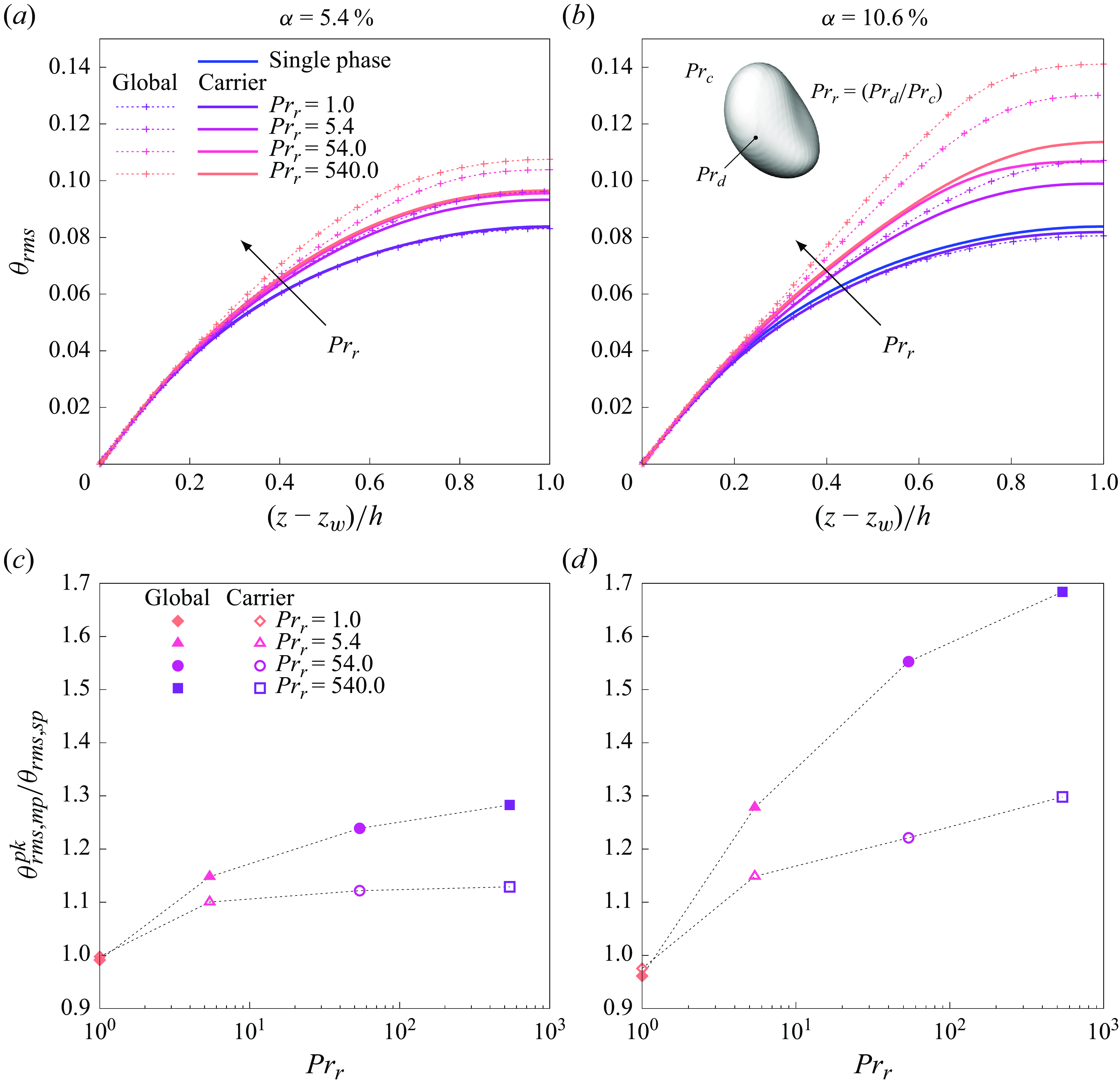
So far, we have discussed the turbulent statistics without distinguishing between the dispersed and carrier phases. Figure 8(a,b) show the RMS of the temperature field computed only in the carrier phase as a function of the wall-normal distance in outer units. For comparison, the global RMS values are also shown as dashed-crossed lines. Figure 8(c,d) illustrate the RMS peak at various ${Pr}_r$
normalised by the RMS peak of the single-phase case, for both carrier (empty symbols) and global (filled symbols) statistics. Figures 8(a,c) and 8(b,d) correspond to volume fractions
${Pr}_r$
normalised by the RMS peak of the single-phase case, for both carrier (empty symbols) and global (filled symbols) statistics. Figures 8(a,c) and 8(b,d) correspond to volume fractions $\alpha =5.4\,\%$
and
$\alpha =5.4\,\%$
and $\alpha =10.6\,\%$
, respectively. The RMS in the carrier follows a trend similar to that of the global RMS, starting from zero at the wall, and reaching a local maximum at the channel centre. Increasing
$\alpha =10.6\,\%$
, respectively. The RMS in the carrier follows a trend similar to that of the global RMS, starting from zero at the wall, and reaching a local maximum at the channel centre. Increasing ${Pr}_r$
leads to higher peaks. The case
${Pr}_r$
leads to higher peaks. The case ${Pr}_r=1$
is not different from the single-phase case of
${Pr}_r=1$
is not different from the single-phase case of $\alpha =5.4\,\%$
, whereas it has a lower peak when
$\alpha =5.4\,\%$
, whereas it has a lower peak when $\alpha =10.6\,\%$
. This reduction can be attributed to the influence of the surface tension forces, which become more significant at higher volume fractions due to the increased interfacial area, thereby dampening convective fluctuations. We can observe that the RMS peaks in the carrier phase are less pronounced than the global RMS, though some clear differences can be observed with respect to the single-phase case. These differences can be traced back to the presence of droplets with different thermal diffusivity that generates large temperature gradients – which in turn increases temperature fluctuations – not only in the droplets but also in the carrier. The increased fluctuations observed in the carrier phase can also be linked to the deflection of the heat-flux lines observed in figure 3. Indeed, this effect becomes more pronounced as
$\alpha =10.6\,\%$
. This reduction can be attributed to the influence of the surface tension forces, which become more significant at higher volume fractions due to the increased interfacial area, thereby dampening convective fluctuations. We can observe that the RMS peaks in the carrier phase are less pronounced than the global RMS, though some clear differences can be observed with respect to the single-phase case. These differences can be traced back to the presence of droplets with different thermal diffusivity that generates large temperature gradients – which in turn increases temperature fluctuations – not only in the droplets but also in the carrier. The increased fluctuations observed in the carrier phase can also be linked to the deflection of the heat-flux lines observed in figure 3. Indeed, this effect becomes more pronounced as ${Pr}_r$
is increased, and such deflections identify temperature fluctuations. An argument in favour of this reasoning is that only in the central part of the channel – where the droplets gather – the RMS of the carrier differs from the single-phase one. The effect of the volume fraction is to further enhance this behaviour as a larger part of the domain is occupied by droplets, thus larger deflections of the heat-flux lines occur. From figure 8(a,b), we also observe that the effect of
${Pr}_r$
is increased, and such deflections identify temperature fluctuations. An argument in favour of this reasoning is that only in the central part of the channel – where the droplets gather – the RMS of the carrier differs from the single-phase one. The effect of the volume fraction is to further enhance this behaviour as a larger part of the domain is occupied by droplets, thus larger deflections of the heat-flux lines occur. From figure 8(a,b), we also observe that the effect of ${Pr}_r$
is nonlinear and tends to a plateau. Indeed, the RMS in the carrier for
${Pr}_r$
is nonlinear and tends to a plateau. Indeed, the RMS in the carrier for ${Pr}_r=54$
and
${Pr}_r=54$
and $540$
for the lower volume fraction, shows almost no differences. In contrast, for the higher volume fraction, the plateau is not reached, although the relative difference between the peaks reduces by increasing
$540$
for the lower volume fraction, shows almost no differences. In contrast, for the higher volume fraction, the plateau is not reached, although the relative difference between the peaks reduces by increasing ${Pr}_r$
.
${Pr}_r$
.
The PDFs of the temperature fluctuations inside the drops $\theta ^\prime _{d,i}$
for each
$\theta ^\prime _{d,i}$
for each ${Pr}_r$
considered: (
${Pr}_r$
considered: ( $a$
) the lower volume fraction; (
$a$
) the lower volume fraction; ( $b$
) the higher volume fraction. The fluctuations are computed using as a reference the mean temperature of each droplet. As a reference, the Gaussian distribution is reported with a black dash-dotted line.
$b$
) the higher volume fraction. The fluctuations are computed using as a reference the mean temperature of each droplet. As a reference, the Gaussian distribution is reported with a black dash-dotted line.

Finally, we analyse the temperature fluctuations inside the droplets. To better characterise these fluctuations, we consider the probability density function (PDFs) of the temperature fluctuations. Figure 9 shows the resulting PDFs as functions of ${Pr}_r$
(distinguished by different colours) and volume fraction (
${Pr}_r$
(distinguished by different colours) and volume fraction ( $\alpha =5.4\,\%$
and
$\alpha =5.4\,\%$
and $10.6\,\%$
), where the black dash-dotted line is the Gaussian distribution, which serves as a reference. We define the fluctuation inside the drop as
$10.6\,\%$
), where the black dash-dotted line is the Gaussian distribution, which serves as a reference. We define the fluctuation inside the drop as
 \begin{equation} \theta _{d,i}^\prime = \theta _{d,i} - \overline {\theta }_{d,i} , \end{equation}
where $\theta _{d,i}$
is the instantaneous temperature, and
$\theta _{d,i}$
is the instantaneous temperature, and $\overline {\theta }_{d,i}$
is the mean temperature of the
$\overline {\theta }_{d,i}$
is the mean temperature of the $i$
th droplet. Since turbulence advects the droplets, they can have a different mean temperature than in the carrier phase. Thus we first identify each drop and compute the temperature fluctuations relative to their own mean temperature. Droplet identification is performed using the algorithm developed by Herrmann (Reference Herrmann2010) that allows us to recognise any contiguous liquid structure. While this method is computationally slower than some recursive approaches, its ability to be parallelised improves performance. The resulting PDFs are symmetric around zero, indicating an equal probability of positive and negative fluctuations. It is worth noticing that despite the symmetric behaviour, the PDFs do not follow the normal distribution. The flatness of the PDFs increases with
$i$
th droplet. Since turbulence advects the droplets, they can have a different mean temperature than in the carrier phase. Thus we first identify each drop and compute the temperature fluctuations relative to their own mean temperature. Droplet identification is performed using the algorithm developed by Herrmann (Reference Herrmann2010) that allows us to recognise any contiguous liquid structure. While this method is computationally slower than some recursive approaches, its ability to be parallelised improves performance. The resulting PDFs are symmetric around zero, indicating an equal probability of positive and negative fluctuations. It is worth noticing that despite the symmetric behaviour, the PDFs do not follow the normal distribution. The flatness of the PDFs increases with ${Pr}_r$
, implying a greater likelihood of extreme temperature deviations from the mean value. At higher volume fractions, the range of
${Pr}_r$
, implying a greater likelihood of extreme temperature deviations from the mean value. At higher volume fractions, the range of $\theta _{d,i}^\prime$
values increases further, confirming that the intensity of temperature fluctuations depends on both
$\theta _{d,i}^\prime$
values increases further, confirming that the intensity of temperature fluctuations depends on both ${Pr}_r$
(i.e. the dissipative time scales) and the volume fraction.
${Pr}_r$
(i.e. the dissipative time scales) and the volume fraction.
(a,b) Scatter plots of the mean temperature of each drop $\overline {\theta }_{d,i}$
against its equivalent diameter normalised by the Kolmogorov–Hinze scale
$\overline {\theta }_{d,i}$
against its equivalent diameter normalised by the Kolmogorov–Hinze scale $d_{eq}^+/d_H^+$
. (c,d) Scatter plots of the RMS of the temperature of each drop against its normalised equivalent diameter. The scatter plots are computed from a single time step at
$d_{eq}^+/d_H^+$
. (c,d) Scatter plots of the RMS of the temperature of each drop against its normalised equivalent diameter. The scatter plots are computed from a single time step at $t^+=3000$
. Each dot identifies a single droplet, while the colours are used to distinguish among the different
$t^+=3000$
. Each dot identifies a single droplet, while the colours are used to distinguish among the different ${Pr}_r$
. Here, (a,c)
${Pr}_r$
. Here, (a,c) $\alpha =5.4\,\%$
, and (b,d)
$\alpha =5.4\,\%$
, and (b,d) $\alpha =10.6\,\%$
.
$\alpha =10.6\,\%$
.

While figure 9 provides insights into the statistical distribution of temperature fluctuations, it does not account for the influence of droplet size. To address this, figure 10 presents scatter plots that shows the effect of the droplet size on the temperature. Figure 10(a,b) show the mean temperature of each droplet as a function of the equivalent diameter normalised by the Kolmogorov–Hinze scale, while figure 10(c,d) display the RMS of temperature over the same normalised diameter. Figure 10(a,c) correspond to the lower volume fraction, $\alpha =5.4\,\%$
, whereas figure 10(b,d) represent the higher volume fraction,
$\alpha =5.4\,\%$
, whereas figure 10(b,d) represent the higher volume fraction, $\alpha =10.6\,\%$
. Different colours denote different
$\alpha =10.6\,\%$
. Different colours denote different ${Pr}_r$
values. Each point in these plots corresponds to an individual droplet at
${Pr}_r$
values. Each point in these plots corresponds to an individual droplet at $t^+ = 3000$
, indicating that the statistics are derived from an instantaneous snapshot rather than time-averaged data.
$t^+ = 3000$
, indicating that the statistics are derived from an instantaneous snapshot rather than time-averaged data.
Examining figure 10(a,b), we observe that smaller droplets span the entire temperature range, whereas larger drops tend to cluster around a mean temperature closer to zero. This behaviour is corroborated by a previous study of Mangani et al. (Reference Mangani, Soligo, Roccon and Soldati2022), where it was shown that small droplets tend to disperse more along the wall-normal direction, i.e. experiencing the whole range of temperature. In contrast, larger drops tend to cluster at the channel centre, where the mean temperature is approximately zero. Notably, ${Pr}_r$
does not appear to influence the mean temperature distribution. Similarly, the volume fraction has only a marginal effect, primarily by altering the maximum droplet size. On the other hand, larger droplets consistently exhibit higher RMS values across all considered
${Pr}_r$
does not appear to influence the mean temperature distribution. Similarly, the volume fraction has only a marginal effect, primarily by altering the maximum droplet size. On the other hand, larger droplets consistently exhibit higher RMS values across all considered ${Pr}_r$
, as shown in figure 10(c,d). This explains the differences observed in figures 7 and 8, where the RMS increases with volume fraction. The
${Pr}_r$
, as shown in figure 10(c,d). This explains the differences observed in figures 7 and 8, where the RMS increases with volume fraction. The ${Pr}_r$
value increases the RMS value for the whole range of diameters (as shown by the arrow in figure 10
c,d), with more pronounced effects on larger drops. Indeed, a layering of the points as a function of the
${Pr}_r$
value increases the RMS value for the whole range of diameters (as shown by the arrow in figure 10
c,d), with more pronounced effects on larger drops. Indeed, a layering of the points as a function of the ${Pr}_r$
value considered can be appreciated.
${Pr}_r$
value considered can be appreciated.
3.4. Heat-flux budget
To characterise the physical mechanisms governing the heat transfer process, we decompose the global heat flux into carrier and dispersed phase contributions. We follow the approach used by Marchioro, Tanksley & Prosperetti (Reference Marchioro, Tanksley and Prosperetti1999), Zhang & Prosperetti (Reference Zhang and Prosperetti2010) and Picano, Breugem & Brandt (Reference Picano, Breugem and Brandt2015) for the total stress balance in suspensions of rigid spherical particles, and by Ardekani et al. (Reference Ardekani, Abouali, Picano and Brandt2018) and Bilondi et al. (Reference Bilondi, Scapin, Brandt and Mirbod2024) for heat transfer in laminar Couette flow with particle suspensions and two-phase turbulent Rayleigh–Bénard convection, respectively. We express the total heat flux as
 \begin{equation} q^{\prime \prime }_{tot} = q^{\prime \prime }_C + q^{\prime \prime }_D , \end{equation}
where $q^{\prime \prime }_C=C_c+C_d$
represents the convective heat flux, given by the sum of the carrier phase
$q^{\prime \prime }_C=C_c+C_d$
represents the convective heat flux, given by the sum of the carrier phase $C_c$
and dispersed phase
$C_c$
and dispersed phase $C_d$
contributions, while
$C_d$
contributions, while $q^{\prime \prime }_D =D_c+D_d$
represents the diffusive heat flux, similarly decomposed into carrier
$q^{\prime \prime }_D =D_c+D_d$
represents the diffusive heat flux, similarly decomposed into carrier $D_c$
and dispersed phase
$D_c$
and dispersed phase $D_d$
contributions. The contributions from each phase are computed as follows:
$D_d$
contributions. The contributions from each phase are computed as follows:
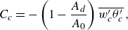 \begin{align}&\quad\, C_c = -\left ( 1-\frac {A_d}{A_0} \right ) \overline {w^\prime _c\theta ^\prime _c} \, , \end{align}
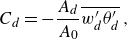 \begin{align}&\qquad\quad C_d = -\frac {A_d}{A_0} \overline {w^\prime _d\theta ^\prime _d} \, , \end{align}
 \begin{align}& D_c = \frac {1}{Re_\tau\, Pr_c}\left ( 1-\frac {A_d}{A_0} \right ) \overline {\frac {\partial \theta _c}{\partial z}} \, , \end{align}
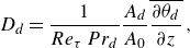 \begin{align}&\quad\,\,\, D_d = \frac {1}{Re_\tau\, Pr_d}\frac {A_d}{A_0} \overline {\frac {\partial \theta _d}{\partial z}}\, , \end{align}
where the subscripts $c$
and
$c$
and $d$
denote the carrier and dispersed phases, respectively. Here,
$d$
denote the carrier and dispersed phases, respectively. Here, $A_d$
represents the average area distribution of the drops, while
$A_d$
represents the average area distribution of the drops, while $A_0$
is the area of a cross-section parallel to the channel walls.
$A_0$
is the area of a cross-section parallel to the channel walls.
Heat-flux budget in the wall-normal direction for the different ${Pr}_r$
considered in this work. The heat fluxes are the sum of the carrier and dispersed phase contributions normalised by the total heat flux of the single-phase case. Each colour refers to a different
${Pr}_r$
considered in this work. The heat fluxes are the sum of the carrier and dispersed phase contributions normalised by the total heat flux of the single-phase case. Each colour refers to a different ${Pr}_r$
, for volume fractions (a)
${Pr}_r$
, for volume fractions (a) $\alpha =5.4\,\%$
and (b)
$\alpha =5.4\,\%$
and (b) $\alpha=10.6\,\%$
.
$\alpha=10.6\,\%$
.
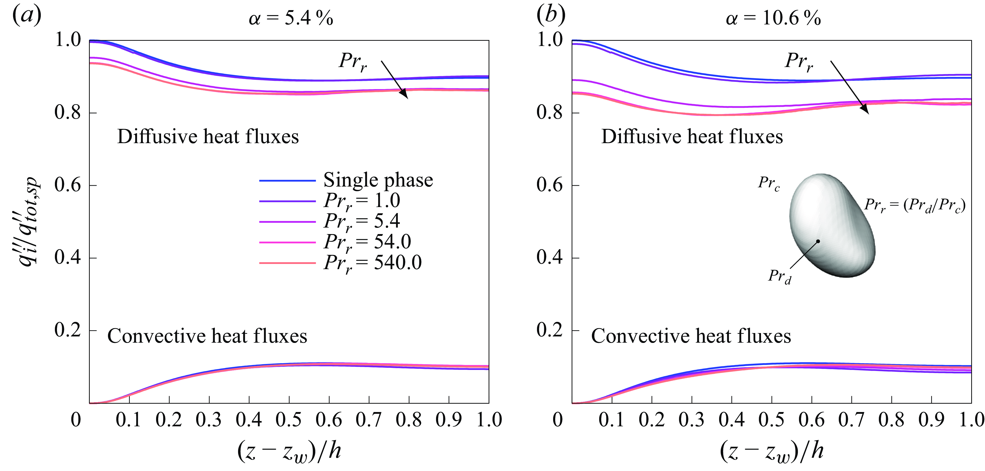
Figure 11 depicts the wall-normal profiles of the convective contribution $q^{\prime \prime }_C$
and diffusive contribution
$q^{\prime \prime }_C$
and diffusive contribution $q^{\prime \prime }_D$
, normalised by the total heat flux of the single-phase case
$q^{\prime \prime }_D$
, normalised by the total heat flux of the single-phase case $q^{\prime \prime }_{tot,sp}$
for the two volume fractions considered,
$q^{\prime \prime }_{tot,sp}$
for the two volume fractions considered, $\alpha =5.4\,\%$
and
$\alpha =5.4\,\%$
and $10.6\,\%$
. At the walls, both velocity and temperature fluctuations are zero, meaning that diffusion is the sole heat transfer mechanism. Moving away from the wall, a reduction of the diffusive heat fluxes is followed by a growth of the convective heat fluxes. However, it is evident that for all
$10.6\,\%$
. At the walls, both velocity and temperature fluctuations are zero, meaning that diffusion is the sole heat transfer mechanism. Moving away from the wall, a reduction of the diffusive heat fluxes is followed by a growth of the convective heat fluxes. However, it is evident that for all ${Pr}_r$
considered, diffusion dominates convection, confirming the previous observation of a conductive thermal sublayer spanning the entire channel width. It is worth noting that the diffusive heat transfer is non-zero at the channel centre due to the presence of a temperature gradient. Normalising by
${Pr}_r$
considered, diffusion dominates convection, confirming the previous observation of a conductive thermal sublayer spanning the entire channel width. It is worth noting that the diffusive heat transfer is non-zero at the channel centre due to the presence of a temperature gradient. Normalising by $q^{\prime \prime }_{tot,sp}$
highlights the overall reduction of the total heat flux when the dispersed phase is introduced, as also observed from the time evolution of the Nusselt number (figure 5). The convective heat fluxes (bottom) are almost not affected by the volume fraction or by
$q^{\prime \prime }_{tot,sp}$
highlights the overall reduction of the total heat flux when the dispersed phase is introduced, as also observed from the time evolution of the Nusselt number (figure 5). The convective heat fluxes (bottom) are almost not affected by the volume fraction or by ${Pr}_r$
. As a matter of fact, the turbulent heat fluxes
${Pr}_r$
. As a matter of fact, the turbulent heat fluxes $q^{\prime \prime }_C$
depend on both the turbulence intensity and the temperature fluctuations. Although increasing the
$q^{\prime \prime }_C$
depend on both the turbulence intensity and the temperature fluctuations. Although increasing the ${Pr}_r$
enhances the temperature fluctuations at the channel centre (in both phases), velocity fluctuations remain one order of magnitude larger, making the effect of
${Pr}_r$
enhances the temperature fluctuations at the channel centre (in both phases), velocity fluctuations remain one order of magnitude larger, making the effect of ${Pr}_r$
almost negligible. Analysing the diffusive contributions (top), a clear effect of the volume fraction and
${Pr}_r$
almost negligible. Analysing the diffusive contributions (top), a clear effect of the volume fraction and ${Pr}_r$
is observed. For both volume fractions, an increase of
${Pr}_r$
is observed. For both volume fractions, an increase of ${Pr}_r$
leads to a reduction of the diffusive heat flux. This modification is visible for
${Pr}_r$
leads to a reduction of the diffusive heat flux. This modification is visible for $\alpha =5.4\,\%$
and becomes more pronounced for
$\alpha =5.4\,\%$
and becomes more pronounced for $\alpha =10.6\,\%$
. This change tends to saturate for
$\alpha =10.6\,\%$
. This change tends to saturate for ${Pr}_r \gt 5.4$
, where results collapse on top of each other for
${Pr}_r \gt 5.4$
, where results collapse on top of each other for ${Pr}_r=54$
and
${Pr}_r=54$
and ${Pr}_r=540$
.
${Pr}_r=540$
.
The wall-normal integrals of (a,b) the convective heat fluxes, and (c,d) the diffusive heat fluxes. All the heat fluxes are reported normalised by the single-phase value. Plots (a,b) show the convective contributions of the carrier (light orange) and dispersed (dark orange) phases. Plots (c,d) show the diffusive contributions of the carrier (light violet) and dispersed (dark violet) phases. Here, (a,c) $\alpha =5.4\,\%$
, and (b,d)
$\alpha =5.4\,\%$
, and (b,d) $\alpha =10.6\,\%$
.
$\alpha =10.6\,\%$
.
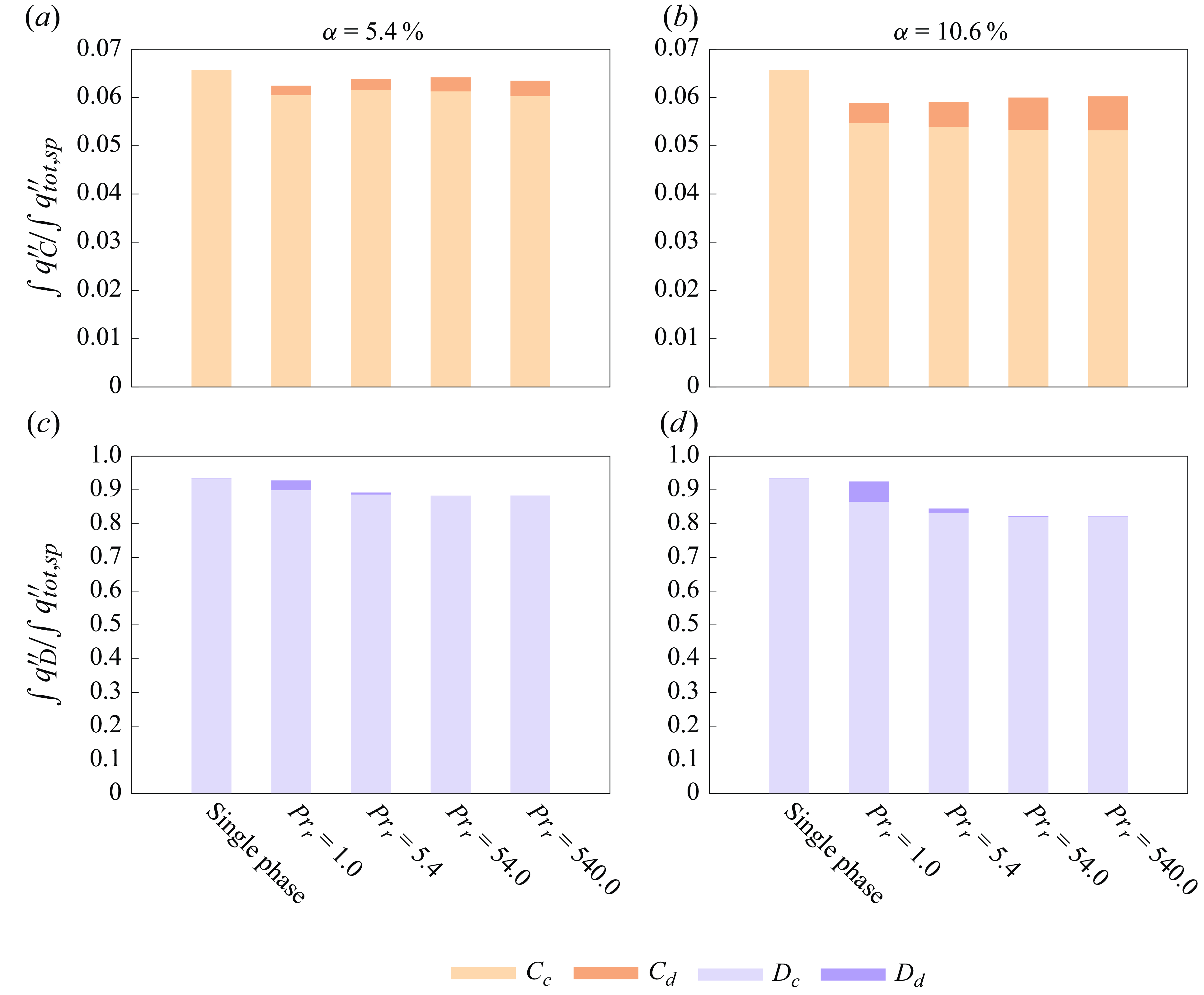
To quantify the impact of these modifications on the global heat-flux performance, we present their integrals normalised by the total heat flux of the single-phase case $q^{\prime \prime }_{tot,sp}$
in figure 12. In particular, the plots illustrate the contributions of the different terms presented in (3.6a
)–(3.6d
). Figure 12(a,b) show the convective heat flux of the dispersed phase (dark orange) and carrier (light orange). Similarly, figure 12(c,d) represent the diffusive heat flux for the dispersed phase (dark violet) and carrier (light violet). Figure 12(a,c) correspond to
$q^{\prime \prime }_{tot,sp}$
in figure 12. In particular, the plots illustrate the contributions of the different terms presented in (3.6a
)–(3.6d
). Figure 12(a,b) show the convective heat flux of the dispersed phase (dark orange) and carrier (light orange). Similarly, figure 12(c,d) represent the diffusive heat flux for the dispersed phase (dark violet) and carrier (light violet). Figure 12(a,c) correspond to $\alpha =5.4\,\%$
, while figure 12(b,d) correspond to
$\alpha =5.4\,\%$
, while figure 12(b,d) correspond to $\alpha =10.6\,\%$
.
$\alpha =10.6\,\%$
.
We start by analysing the convective contributions (figure 12
a,b). As ${Pr}_r$
increases, local temperature gradients generate stronger fluctuations in both the carrier and droplets (as shown in figures 7 and 8). However, the increased temperature fluctuations (higher RMS) do not translate into a higher global convective heat flux. Statistically, the combined contributions of the carrier and dispersed phases remain lower than in the single-phase case and show no significant dependence on
${Pr}_r$
increases, local temperature gradients generate stronger fluctuations in both the carrier and droplets (as shown in figures 7 and 8). However, the increased temperature fluctuations (higher RMS) do not translate into a higher global convective heat flux. Statistically, the combined contributions of the carrier and dispersed phases remain lower than in the single-phase case and show no significant dependence on ${Pr}_r$
. On the other hand, for each value of
${Pr}_r$
. On the other hand, for each value of ${Pr}_r$
, the average convective heat flux associated with the dispersed phase increases with volume fraction. Further discussion of the statistical analysis and uncertainty estimation is provided in Appendix B. It is important to observe that the convective heat fluxes account for less than
${Pr}_r$
, the average convective heat flux associated with the dispersed phase increases with volume fraction. Further discussion of the statistical analysis and uncertainty estimation is provided in Appendix B. It is important to observe that the convective heat fluxes account for less than $7\,\%$
of the global heat flux.
$7\,\%$
of the global heat flux.
Moving to the diffusive contributions (figure 12
c,d), diffusion in the carrier phase decreases for all the multiphase cases. For ${Pr}_r=1$
, the reduction is balanced by an increase in diffusion within the dispersed phase, resulting in a minimal net effect. As
${Pr}_r=1$
, the reduction is balanced by an increase in diffusion within the dispersed phase, resulting in a minimal net effect. As ${Pr}_r$
increases, diffusion in the carrier phase decreases further without a corresponding compensation in the dispersed phase. As a consequence, the overall diffusive heat flux decreases with both
${Pr}_r$
increases, diffusion in the carrier phase decreases further without a corresponding compensation in the dispersed phase. As a consequence, the overall diffusive heat flux decreases with both ${Pr}_r$
and volume fraction.
${Pr}_r$
and volume fraction.
3.5. Phenomenological model for the Nusselt number
Mean Nusselt number $\textit {Nu}$
normalised with the average value of the single phase
$\textit {Nu}$
normalised with the average value of the single phase $\textit {Nu}_{s}$
as a function of
$\textit {Nu}_{s}$
as a function of ${Pr}_r$
for two distinct volume fractions,
${Pr}_r$
for two distinct volume fractions, $\alpha =5.4\,\%$
and
$\alpha =5.4\,\%$
and $10.6\,\%$
. The filled symbols represent the DNS data, while the black dashed lines report the predictions obtained from the proposed model (3.13). The error bars represent the RMS of the Nusselt number.
$10.6\,\%$
. The filled symbols represent the DNS data, while the black dashed lines report the predictions obtained from the proposed model (3.13). The error bars represent the RMS of the Nusselt number.
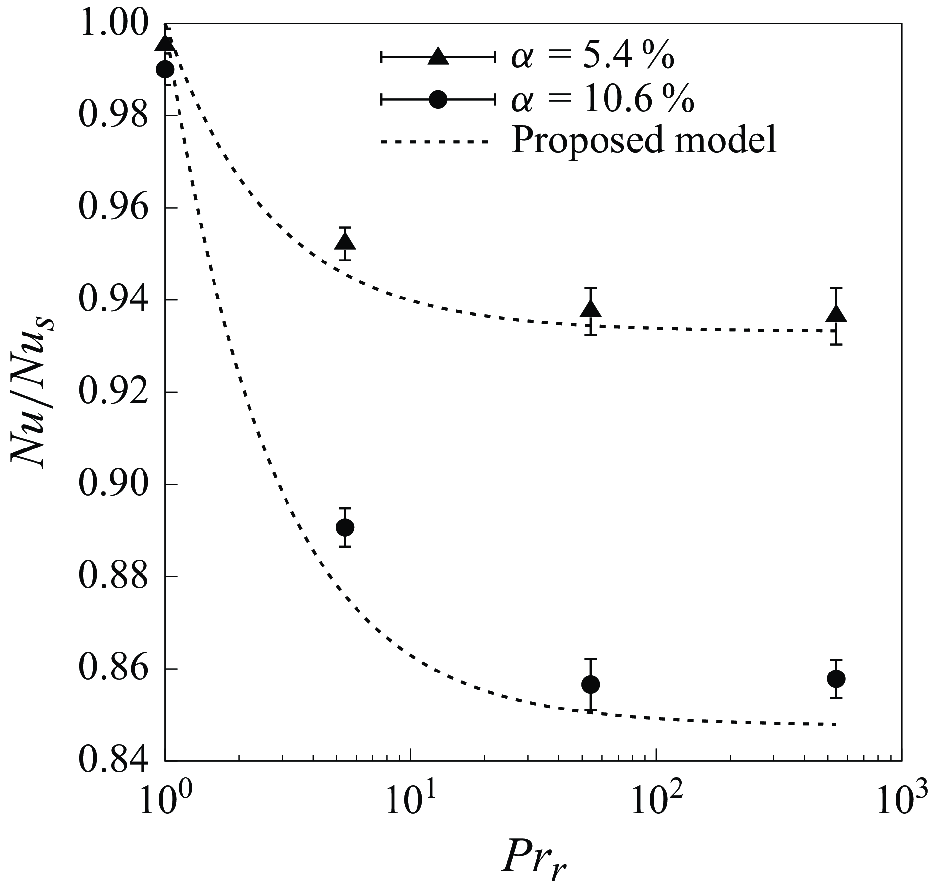
Having identified the physical mechanism governing heat transfer, we can try to model the corresponding process. In particular, we want to build a one-dimensional model that predicts the global heat transfer of low-Prandtl-number drop-laden flows. To this aim, we recall the time evolution of the Nusselt number presented in figure 5, and we focus on the steady values attained by the different cases for $t^+\gt 1000$
, which are reported in figure 13. The results for volume fractions
$t^+\gt 1000$
, which are reported in figure 13. The results for volume fractions $\alpha =5.4\,\%$
and
$\alpha =5.4\,\%$
and $10.6\,\%$
are represented by solid triangles and solid circles, respectively. We observe that for both volume fractions considered,
$10.6\,\%$
are represented by solid triangles and solid circles, respectively. We observe that for both volume fractions considered, $\textit {Nu}$
decreases with a nonlinear trend, eventually reaching a plateau for
$\textit {Nu}$
decreases with a nonlinear trend, eventually reaching a plateau for ${Pr}_r \gt 54$
. Likewise, an increase in the the volume fraction leads to a drop of the Nusselt number. For instance, the case with
${Pr}_r \gt 54$
. Likewise, an increase in the the volume fraction leads to a drop of the Nusselt number. For instance, the case with $\alpha =5.4\,\%$
(
$\alpha =5.4\,\%$
( ${Pr}_r=540$
) exhibits a higher total heat flux than the case with
${Pr}_r=540$
) exhibits a higher total heat flux than the case with $\alpha =10.6\,\%$
(
$\alpha =10.6\,\%$
( ${Pr}_r=5.4$
).
${Pr}_r=5.4$
).
To develop the model, we start by integrating the right-hand side of (2.10) over the entire channel, and normalising it by the single-phase value:
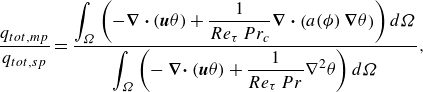 \begin{equation} \frac {q_{tot,mp}}{q_{tot,sp}} = \frac {\displaystyle\int _\Omega \left ( -\boldsymbol{\nabla } \boldsymbol{\cdot } ( \boldsymbol{u}\theta ) + \frac {1}{Re_\tau\, Pr_c} \boldsymbol{\nabla } \boldsymbol{\cdot } \big ( a(\phi )\, \boldsymbol{\nabla } \theta \big ) \right ) {d}\Omega }{\displaystyle \int _\Omega \left ( -\boldsymbol{ \nabla \cdot } ( \boldsymbol{u}\theta ) + \frac {1}{Re_\tau\, Pr} \nabla ^2 \theta \right ) {d}\Omega } , \end{equation}
where ${d}\Omega$
is the elemental volume within the control volume
${d}\Omega$
is the elemental volume within the control volume $\Omega$
. Since both
$\Omega$
. Since both ${Pr}_r$
and
${Pr}_r$
and $\alpha$
have a minor effect on the convective heat fluxes – and these fluxes account for less than
$\alpha$
have a minor effect on the convective heat fluxes – and these fluxes account for less than $7\,\%$
of the total heat transfer, as discussed in figures 11 and 12 – we assume that the convective heat fluxes are negligible. Applying this assumption and applying Gauss’ theorem to (3.7), we obtain
$7\,\%$
of the total heat transfer, as discussed in figures 11 and 12 – we assume that the convective heat fluxes are negligible. Applying this assumption and applying Gauss’ theorem to (3.7), we obtain
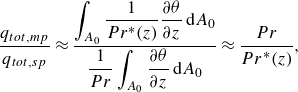 \begin{equation} \frac {q_{tot,mp}}{q_{tot,sp}} \approx \frac {\displaystyle \int _{A_0} \frac {1}{Pr^\ast (z)} \frac {\partial \theta }{\partial z}\, {\textrm d}A_0 }{\displaystyle \frac {1}{ Pr} \int _{A_0} \frac {\partial \theta }{\partial z}\, {\textrm d}A_0 } \approx \frac {Pr}{Pr^\ast (z)} , \end{equation}
where ${Pr}^\ast (z) = Pr_c/a(\phi )$
is function of the wall-normal elevation. We further simplify (3.8) considering that
${Pr}^\ast (z) = Pr_c/a(\phi )$
is function of the wall-normal elevation. We further simplify (3.8) considering that $\partial \theta /\partial z \approx 1$
for all the cases under scrutiny. It is important to note that due to Gauss’ theorem, only the heat-flux component normal to the oriented area
$\partial \theta /\partial z \approx 1$
for all the cases under scrutiny. It is important to note that due to Gauss’ theorem, only the heat-flux component normal to the oriented area $A_0$
contributes to the total heat flux. Hence reducing the conductivity efficiency inside the dispersed phase corresponds to reducing the area of effective heat transport. Based on this, it is reasonable to model
$A_0$
contributes to the total heat flux. Hence reducing the conductivity efficiency inside the dispersed phase corresponds to reducing the area of effective heat transport. Based on this, it is reasonable to model ${Pr}^\ast (z)$
as a function of the area occupied by the carrier and the dispersed phase, namely a function of the wall-normal distance. We take advantage of the analogy with the conduction in layered media presented in Appendix A, and write
${Pr}^\ast (z)$
as a function of the area occupied by the carrier and the dispersed phase, namely a function of the wall-normal distance. We take advantage of the analogy with the conduction in layered media presented in Appendix A, and write
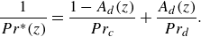 \begin{equation} \frac {1}{Pr^\ast (z)} = \frac {1-A_d(z)}{Pr_c}+ \frac {A_d(z)}{Pr_d}. \end{equation}
( $a$
) The average area distribution of the drops
$a$
) The average area distribution of the drops $A_d$
in the wall-normal direction normalised by the area of a channel section
$A_d$
in the wall-normal direction normalised by the area of a channel section $A_0$
for two volume fractions. (
$A_0$
for two volume fractions. ( $b$
) The average area distribution of the drops rescaled by their respective maximum value
$b$
) The average area distribution of the drops rescaled by their respective maximum value $A_{d,\textit {max}}$
. The dashed black lines represent a Gaussian function.
$A_{d,\textit {max}}$
. The dashed black lines represent a Gaussian function.
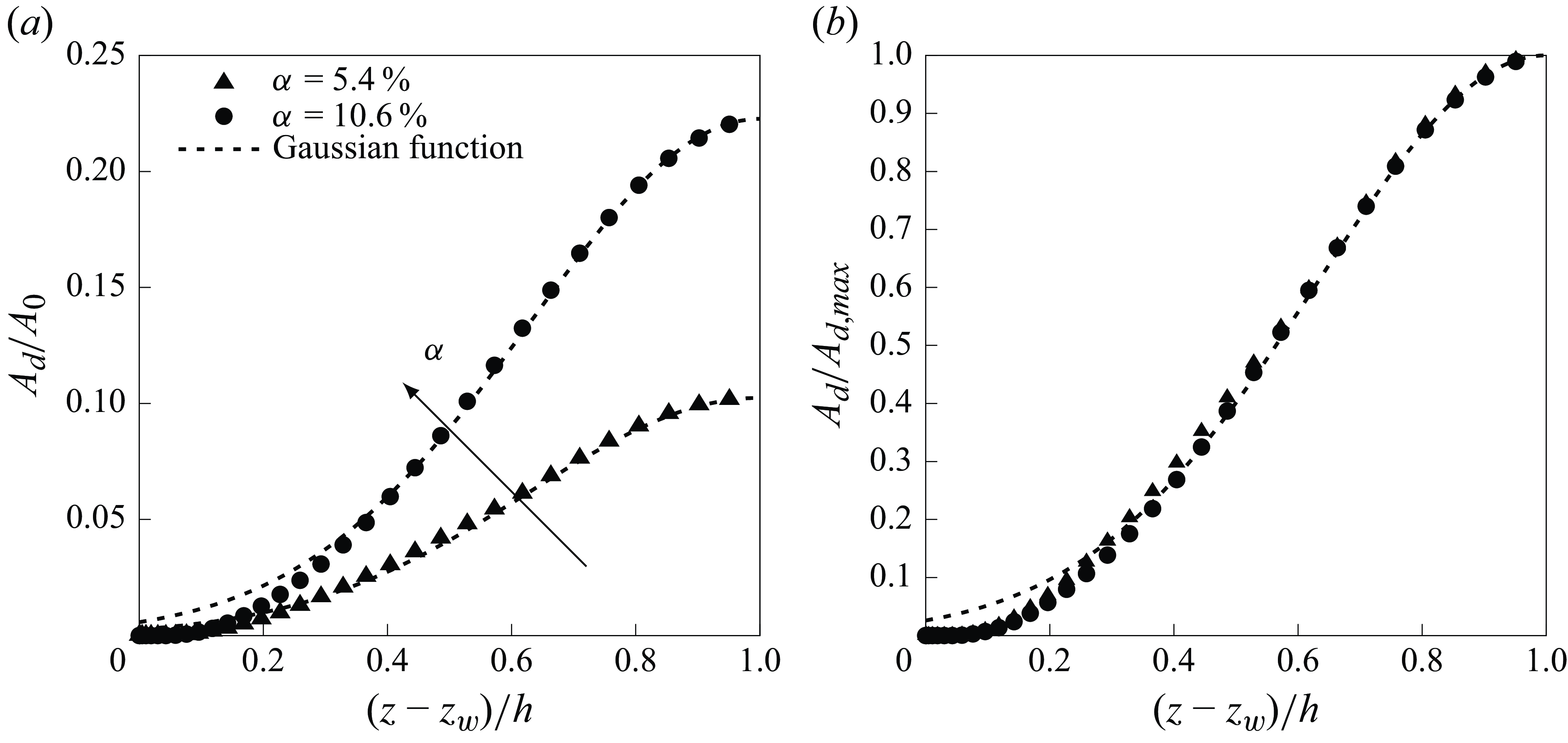
Figure 14 shows the wall-normal distribution of the dispersed area for volume fractions $\alpha =5.4\,\%$
(solid triangles) and
$\alpha =5.4\,\%$
(solid triangles) and $10.6\,\%$
(solid circles). Figure 14(a) shows the drop area normalised by the total area, while figure 14(b) presents the drop area normalised by its maximum value. The plotted data represent an average over all simulations. As expected, increasing the volume fraction leads to a larger dispersed phase area. The droplets are gathered at the channel centre (Mangani et al. Reference Mangani, Soligo, Roccon and Soldati2022). Rescaling the drop area by its maximum value reveals a self-similar behaviour across the volume fractions considered in this study. Hence both distributions can be described using an analytical function with
$10.6\,\%$
(solid circles). Figure 14(a) shows the drop area normalised by the total area, while figure 14(b) presents the drop area normalised by its maximum value. The plotted data represent an average over all simulations. As expected, increasing the volume fraction leads to a larger dispersed phase area. The droplets are gathered at the channel centre (Mangani et al. Reference Mangani, Soligo, Roccon and Soldati2022). Rescaling the drop area by its maximum value reveals a self-similar behaviour across the volume fractions considered in this study. Hence both distributions can be described using an analytical function with $A_{d,\textit {max}}$
as a scaling parameter. After systematically evaluating candidate functions, we find that the Gaussian function provides the best description of
$A_{d,\textit {max}}$
as a scaling parameter. After systematically evaluating candidate functions, we find that the Gaussian function provides the best description of $A_d$
:
$A_d$
:
 \begin{equation} A_d(z) \approx a \exp\left( {-\frac {(z-b)^2}{2c^2}} \right) , \end{equation}
where $a=\max (A_d)=A_{d,\textit {max}}$
,
$a=\max (A_d)=A_{d,\textit {max}}$
, $b=0$
is the mean value of
$b=0$
is the mean value of $A_d/A_{d,\textit {max}}$
, and
$A_d/A_{d,\textit {max}}$
, and $c=\textrm{std}(A_d/A_{d,max}) \approx 0.37$
is the standard deviation of
$c=\textrm{std}(A_d/A_{d,max}) \approx 0.37$
is the standard deviation of $A_d/A_{d,\textit {max}}$
. The Gaussian fit is reported in figure 14 with a dashed line. Notice that the area distribution is well represented throughout the channel width, with minor discrepancies near the wall. However, these deviations occur in regions where small droplets appear intermittently. As already discussed for figure 10, small droplets have little to no influence on the heat-flux budget.
$A_d/A_{d,\textit {max}}$
. The Gaussian fit is reported in figure 14 with a dashed line. Notice that the area distribution is well represented throughout the channel width, with minor discrepancies near the wall. However, these deviations occur in regions where small droplets appear intermittently. As already discussed for figure 10, small droplets have little to no influence on the heat-flux budget.
Normalised Nusselt number rescaled by the maximum value of the drops area as a function of ${Pr}_d$
. The black dashed line represents the proposed model.
${Pr}_d$
. The black dashed line represents the proposed model.
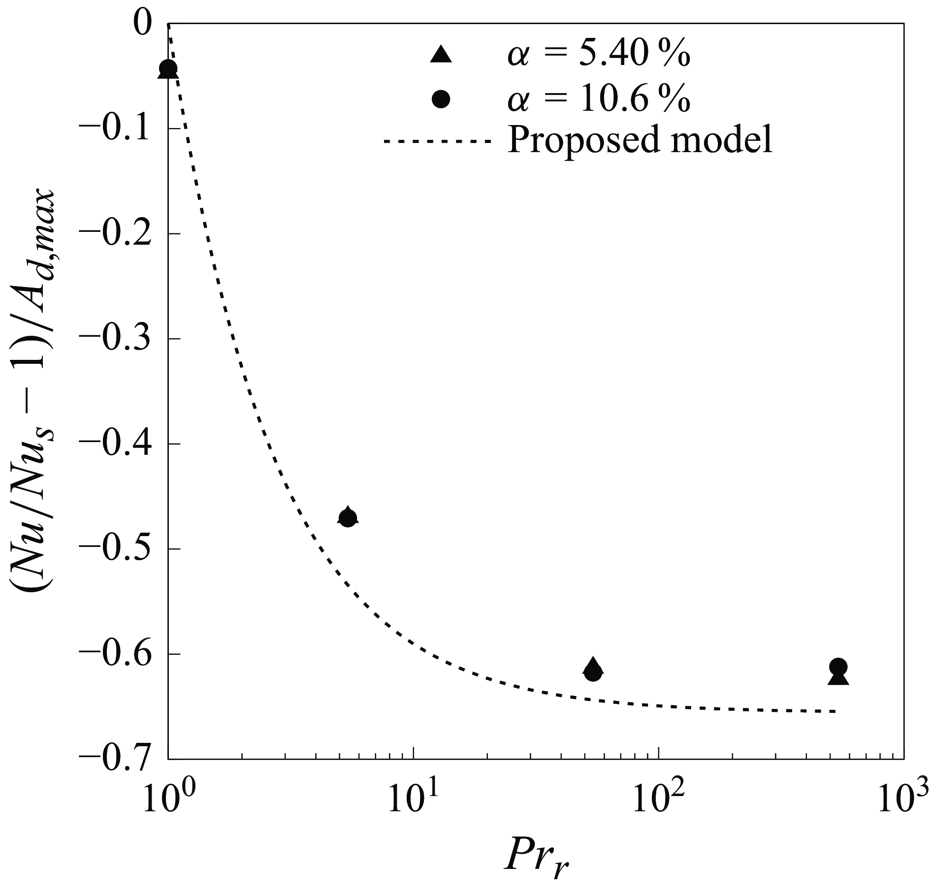
An equivalent global thermal resistance of the multiphase system – i.e. the equivalent Prandtl number ${Pr}_{{eqv}}$
– can be determined by averaging
${Pr}_{{eqv}}$
– can be determined by averaging $1/Pr^{\ast }$
between the two walls:
$1/Pr^{\ast }$
between the two walls:
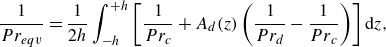 \begin{equation} \frac {1}{Pr_{eqv}} = \frac {1}{2h} \int _{-h}^{+h} \left [ \frac {1}{Pr_c} + A_d(z) \left ( \frac {1}{Pr_d} - \frac {1}{Pr_c} \right ) \right ] {\textrm d}z, \end{equation}
where $A_d(z)$
is explicitly factored out. Substituting (3.10) into (3.11) yields
$A_d(z)$
is explicitly factored out. Substituting (3.10) into (3.11) yields
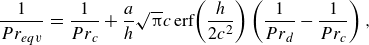 \begin{eqnarray} \frac {1}{Pr_{eqv}} &=& \frac {1}{Pr_c} + \frac {a}{h}\sqrt {{\unicode[Arial]{x03C0}} }c \, \textrm {erf}{\left ( \frac {h}{2c^2} \right )} \left ( \frac {1}{Pr_d} - \frac {1}{Pr_c} \right ) , \end{eqnarray}
where $\textrm{erf}{(h/(2c^2))}\sim 1$
is the error function. With
$\textrm{erf}{(h/(2c^2))}\sim 1$
is the error function. With ${Pr}_{eqv}$
now representing the average conductivity of the two-phase system, we estimate (3.8) at the wall. Recalling that the non-dimensional heat flux at the wall is the Nusselt number
${Pr}_{eqv}$
now representing the average conductivity of the two-phase system, we estimate (3.8) at the wall. Recalling that the non-dimensional heat flux at the wall is the Nusselt number $Nu$
, the final model is
$Nu$
, the final model is
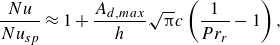 \begin{equation} \frac {{Nu}}{{Nu}_{sp}} \approx 1+ \frac {A_{d,{max}}}{h}\sqrt {{\unicode[Arial]{x03C0}} }c \left ( \frac {1}{Pr_r} - 1 \right ), \end{equation}
where we substitute $a=A_{d,{max}}$
. This equation shows that the normalised Nusselt number depends on the maximum dispersed phase area and the Prandtl ratio. The model predictions (represented by dashed lines in figure 13) accurately capture the observed trend of
$a=A_{d,{max}}$
. This equation shows that the normalised Nusselt number depends on the maximum dispersed phase area and the Prandtl ratio. The model predictions (represented by dashed lines in figure 13) accurately capture the observed trend of ${Nu}/{Nu}_{sp}$
, confirming its validity in predicting the heat transfer behaviour in multiphase systems. In particular, (3.13) shows that the asymptote observed at high
${Nu}/{Nu}_{sp}$
, confirming its validity in predicting the heat transfer behaviour in multiphase systems. In particular, (3.13) shows that the asymptote observed at high $Pr$
arises from both physical and geometrical effects. Physically, when the dispersed phase becomes sufficiently insulating, further reductions in its conductivity have minimal impact on the total heat flux. Geometrically, the drop distribution influences the relative importance of the drop conductivity in determining the equivalent thermal conductivity of the system.
$Pr$
arises from both physical and geometrical effects. Physically, when the dispersed phase becomes sufficiently insulating, further reductions in its conductivity have minimal impact on the total heat flux. Geometrically, the drop distribution influences the relative importance of the drop conductivity in determining the equivalent thermal conductivity of the system.
Figure 15 shows the DNS results rescaled by $A_{d,{max}}$
. The collapse of the different cases confirms the self-similar behaviour observed for the dispersed phase area. The model slightly underestimates the Nusselt number, primarily due to the assumption that
$A_{d,{max}}$
. The collapse of the different cases confirms the self-similar behaviour observed for the dispersed phase area. The model slightly underestimates the Nusselt number, primarily due to the assumption that $Pr_r$
and
$Pr_r$
and $A_d$
have a negligible impact on the convective terms. As discussed in § 3.4, these contributions increase slightly, leading to a minor discrepancy between the model and the DNS results. Quantitative comparison reveals remarkable agreement between model predictions and DNS results, with relative errors below
$A_d$
have a negligible impact on the convective terms. As discussed in § 3.4, these contributions increase slightly, leading to a minor discrepancy between the model and the DNS results. Quantitative comparison reveals remarkable agreement between model predictions and DNS results, with relative errors below $1.1\,\%$
across all tested conditions (error range between
$1.1\,\%$
across all tested conditions (error range between $0.017\,\%$
and
$0.017\,\%$
and $1.1\,\%$
). Overall, the proposed model is capable of predicting the heat transfer performance of a complex multiphase system for a wide range of
$1.1\,\%$
). Overall, the proposed model is capable of predicting the heat transfer performance of a complex multiphase system for a wide range of $Pr_r$
as well as different values of the dispersed phase volume fraction.
$Pr_r$
as well as different values of the dispersed phase volume fraction.
4. Conclusions
In this work, we investigated the modifications to heat transfer induced by a swarm of deformable droplets in the turbulent flow of low-Prandtl-number fluid ( $Pr_c=0.013$
). The study was conducted using direct numerical simulations (DNS) of Navier–Stokes equations coupled with a phase-field method. The energy equation was one-way coupled, with the Cahn–Hilliard equation to account for the different thermal conductivities of the two phases. We considered a fixed friction Reynolds number (
$Pr_c=0.013$
). The study was conducted using direct numerical simulations (DNS) of Navier–Stokes equations coupled with a phase-field method. The energy equation was one-way coupled, with the Cahn–Hilliard equation to account for the different thermal conductivities of the two phases. We considered a fixed friction Reynolds number ( $Re_\tau =300$
) and Weber number (
$Re_\tau =300$
) and Weber number ( $We=3$
), while varying both the Prandtl ratio and volume fraction. Specifically, we examined four different conductivity ratios, corresponding to
$We=3$
), while varying both the Prandtl ratio and volume fraction. Specifically, we examined four different conductivity ratios, corresponding to $Pr_r=1, 5.4, 54, 540$
, along with two volume fractions,
$Pr_r=1, 5.4, 54, 540$
, along with two volume fractions, $\alpha =5.4\,\%$
and
$\alpha =5.4\,\%$
and $10.6\,\%$
.
$10.6\,\%$
.
First, we characterised the topology of the dispersed phase by analysing the droplet size distribution (DSD). After an initial transient phase (up to $t^+=1000$
), the DSD remains statistically unchanged, revealing two distinct regimes: a breakage-dominated regime (for drops larger than the Kolmogorov–Hinze scale), which follows the scaling
$t^+=1000$
), the DSD remains statistically unchanged, revealing two distinct regimes: a breakage-dominated regime (for drops larger than the Kolmogorov–Hinze scale), which follows the scaling $d^{-10/3}$
; and, a coalescence-dominated regime (for drops smaller than the Kolmogorov–Hinze scale), exhibiting a
$d^{-10/3}$
; and, a coalescence-dominated regime (for drops smaller than the Kolmogorov–Hinze scale), exhibiting a $d^{-3/2}$
scaling. For the higher volume fraction, we observe both a slightly larger presence of larger drops and an increased number of small droplets compared to the lower volume fraction case.
$d^{-3/2}$
scaling. For the higher volume fraction, we observe both a slightly larger presence of larger drops and an increased number of small droplets compared to the lower volume fraction case.
Then we analysed the temperature field from a global perspective and within the two phases. We observed that the global heat transfer, represented by the average Nusselt number (see table 2), reaches a steady-state value once the DSD also stabilised. The presence of a dispersed phase with higher $Pr_d$
(i.e. smaller thermal conductivity) than the carrier phase leads to a reduction in
$Pr_d$
(i.e. smaller thermal conductivity) than the carrier phase leads to a reduction in $\textit {Nu}$
. Similarly, an increase of the volume fraction leads to a decrease of the Nusselt number. Interestingly, while the mean temperature is slightly affected by
$\textit {Nu}$
. Similarly, an increase of the volume fraction leads to a decrease of the Nusselt number. Interestingly, while the mean temperature is slightly affected by $Pr_r$
, the combined effect of
$Pr_r$
, the combined effect of $Pr_r$
and volume fraction leads to more pronounced differences between the mean temperature of the multiphase and single-phase cases. This is confirmed by the temperature RMS, where the presence of the dispersed phase increases fluctuation intensity. Counterintuitively, also the RMS in the carrier phase increases, meaning that local temperature gradients – enhanced by the presence of the dispersed phase – generate larger temperature fluctuations even within the carrier.
$Pr_r$
and volume fraction leads to more pronounced differences between the mean temperature of the multiphase and single-phase cases. This is confirmed by the temperature RMS, where the presence of the dispersed phase increases fluctuation intensity. Counterintuitively, also the RMS in the carrier phase increases, meaning that local temperature gradients – enhanced by the presence of the dispersed phase – generate larger temperature fluctuations even within the carrier.
Overview of the main results. We report, for each case studied, the average Nusselt number $\textit {Nu}$
, the maximum value of the global RMS
$\textit {Nu}$
, the maximum value of the global RMS $(\theta ^{pk}_{rms,g})$
and the maximum value of the RMS in the carrier only
$(\theta ^{pk}_{rms,g})$
and the maximum value of the RMS in the carrier only $(\theta ^{pk}_{rms,c})$
.
$(\theta ^{pk}_{rms,c})$
.
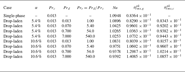
Finally, we analysed the heat-flux budgets, and we observed that the presence of a dispersed phase with different conductivity in a low- $Pr$
carrier reduces the diffusive heat fluxes, while the convective heat fluxes remain mostly unchanged. Building on these observations, we developed a physically grounded model to predict changes in
$Pr$
carrier reduces the diffusive heat fluxes, while the convective heat fluxes remain mostly unchanged. Building on these observations, we developed a physically grounded model to predict changes in $\textit {Nu}$
for varying
$\textit {Nu}$
for varying $Pr_r$
and volume fractions. The model expresses the variation in
$Pr_r$
and volume fractions. The model expresses the variation in $\textit {Nu}$
as a function of the maximum area occupied by the dispersed phase and the Prandtl ratio
$\textit {Nu}$
as a function of the maximum area occupied by the dispersed phase and the Prandtl ratio $Pr_r$
. Model predictions closely match DNS results, and uncover a self-similar behaviour between the two volume fractions considered.
$Pr_r$
. Model predictions closely match DNS results, and uncover a self-similar behaviour between the two volume fractions considered.
Acknowledgements
We acknowledge EURO-HPC JU for awarding us access to LUMI-C@LUMI, Finland (project ID EHPC-EXT-2022E01-003), ISCRA for awarding us access to Leonardo (project ID HP10BUJEO5) and Sigma2 for awarding us access to Betzy (project ID NN9646K). We acknowledge TU Wien for financial support through its Open Access Funding Programme. We thank A. Arosemena and S. Di Giorgio for useful discussions.
Funding
D.P. and J.S. gratefully acknowledge financial support from NTNU. A.R. and A.S. gratefully acknowledge financial support from PRIN 2022, ‘The fluid dynamics of interfaces: mesoscale models for bubbles, droplets, and membranes and their coupling to large scale flows’ (2022R9B2MW - G53C24000810001).
Declaration of interests
The authors report no conflict of interest.
Data availability statement
Data available on request from the authors.
Appendix A. On the analogy with the conduction in layered systems
In this appendix, we analyse the analogy between the conduction problem in layered systems and the heat transfer in multiphase low-Prandtl-number media.
In layered systems (e.g. alternating materials with different conductivities $\kappa _i$
), the layer thermal conductivity
$\kappa _i$
), the layer thermal conductivity $\kappa ^*$
depends on the direction of the heat flux. In particular, when the heat flux is parallel to the layering, we have
$\kappa ^*$
depends on the direction of the heat flux. In particular, when the heat flux is parallel to the layering, we have
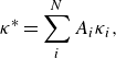 \begin{equation} \kappa ^* = \sum _i^N A_i \kappa _i, \end{equation}
where $A_i$
is the area fractions the
$A_i$
is the area fractions the $i\textrm th$
material layer (Murakami et al. Reference Murakami, Hegemier and Gurtman1980, Reference Murakami, Maewal and Hegemier1981; Baker-Jarvis & Inguva Reference Baker-Jarvis and Inguva1984). It is important to note that this relation is valid in the pure conductive limit. However, in our case, the convection accounts for a maximum of
$i\textrm th$
material layer (Murakami et al. Reference Murakami, Hegemier and Gurtman1980, Reference Murakami, Maewal and Hegemier1981; Baker-Jarvis & Inguva Reference Baker-Jarvis and Inguva1984). It is important to note that this relation is valid in the pure conductive limit. However, in our case, the convection accounts for a maximum of $7\,\%$
of the total heat transfer. Therefore, our case is conduction-dominated. Moreover, the presence of drops with different
$7\,\%$
of the total heat transfer. Therefore, our case is conduction-dominated. Moreover, the presence of drops with different $Pr$
from the carrier does not significantly affect the convection. Thus we can assume that the variation of the total heat flux depends only on the conductive heat-flux reduction.
$Pr$
from the carrier does not significantly affect the convection. Thus we can assume that the variation of the total heat flux depends only on the conductive heat-flux reduction.
With these assumptions, and considering the steady-state condition, we can think of our system as a channel where each cross-section has a property distribution. This case is very similar to the case of heat flux parallel to the layering, as shown in figure 16. Therefore, considering the analogy with the layered systems and that $\kappa _i \propto 1/Pr_i$
, we can write
$\kappa _i \propto 1/Pr_i$
, we can write
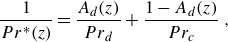 \begin{equation} \frac {1}{Pr^*(z)} = \frac {A_d(z)}{Pr_d} + \frac {1-A_d(z)}{Pr_c} \ , \end{equation}
where $Pr^*$
can be interpreted as the average Prandtl number of the infinitesimal layer parallel to the walls.
$Pr^*$
can be interpreted as the average Prandtl number of the infinitesimal layer parallel to the walls.
Schematic configuration of an infinitesimal portion of the channel. The grey region represents the volume occupied by the drop. The carrier and drop are characterised by different conductivities, i.e. $Pr_c \neq Pr_d$
. The infinitesimal heat flux
$Pr_c \neq Pr_d$
. The infinitesimal heat flux ${\textrm d}q$
is parallel to the layered system (carrier-drop).
${\textrm d}q$
is parallel to the layered system (carrier-drop).
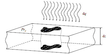
Appendix B. Statistical convergence and uncertainty estimation
To ensure the statistical reliability of the reported heat-flux components, all quantities were computed over the statistically steady portion of the simulations. Each DNS was run for a total duration of $4500\ t^+$
. The initial
$4500\ t^+$
. The initial $1000\ t^+$
were discarded to eliminate the transient phase, and the remaining
$1000\ t^+$
were discarded to eliminate the transient phase, and the remaining $3500\ t^+$
were used for statistical analysis. Data were sampled every
$3500\ t^+$
were used for statistical analysis. Data were sampled every $15\ t^+$
, yielding
$15\ t^+$
, yielding $233$
time samples per case.
$233$
time samples per case.
Autocorrelation function of the Nusselt number, $\rho (\textit {Nu})$
, as a function of the time lag
$\rho (\textit {Nu})$
, as a function of the time lag $\delta t^+$
for the different cases considered. The autocorrelation has been computed starting from
$\delta t^+$
for the different cases considered. The autocorrelation has been computed starting from $t^+=1000$
, i.e. when the simulations reach the steady state. Here, (a)
$t^+=1000$
, i.e. when the simulations reach the steady state. Here, (a) $\alpha =5.4\,\%$
, and (b)
$\alpha =5.4\,\%$
, and (b) $\alpha =10.6\,\%$
.
$\alpha =10.6\,\%$
.
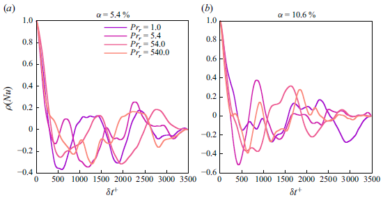
Due to the turbulent nature of the flow, the instantaneous heat-flux contributions exhibit temporal fluctuations. To account for this, we estimate the statistical uncertainty using the standard error of the mean value, corrected for time correlation via the integral autocorrelation time. Specifically, we compute the autocorrelation function (see figure 17) of the total wall-normal heat flux over the steady-state window. The autocorrelation decays smoothly and crosses zero at a lag of approximately $240\ t^+$
for all the cases. By integrating the positive portion of the autocorrelation using the trapezoidal rule, we obtain an integral autocorrelation time
$240\ t^+$
for all the cases. By integrating the positive portion of the autocorrelation using the trapezoidal rule, we obtain an integral autocorrelation time $\tau ^+$
that slightly differs in the different cases. Therefore, we choose the most conservative case where
$\tau ^+$
that slightly differs in the different cases. Therefore, we choose the most conservative case where $\tau ^+ \approx 121.37$
. Given the total duration
$\tau ^+ \approx 121.37$
. Given the total duration $T^+=3500$
, this corresponds to an effective number of independent samples given by
$T^+=3500$
, this corresponds to an effective number of independent samples given by
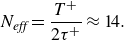 \begin{equation} N_{\textit{eff}} = \frac {T^+}{2\tau ^+} \approx 14. \end{equation}
The estimated standard errors for the convective heat-flux components (carrier and dispersed phases) were computed using the effective sample size. Results are presented in table 3. While the total convective heat flux exhibits limited sensitivity to $Pr_r$
, in many cases, the variation is comparable to the magnitude of the statistical uncertainty. These trends should therefore be interpreted with appropriate caution. However, as shown in figure 18, a consistent and statistically robust increase in the convective heat-flux contribution from the dispersed phase is observed with increasing volume fraction, for all values of
$Pr_r$
, in many cases, the variation is comparable to the magnitude of the statistical uncertainty. These trends should therefore be interpreted with appropriate caution. However, as shown in figure 18, a consistent and statistically robust increase in the convective heat-flux contribution from the dispersed phase is observed with increasing volume fraction, for all values of $Pr_r$
.
$Pr_r$
.
Mean values and standard error for the convective heat-flux contributions of the carrier ( $C_c$
) and dispersed (
$C_c$
) and dispersed ( $C_d$
) phases, computed using effective sample size
$C_d$
) phases, computed using effective sample size $N_{\textit{eff}} = 14$
.
$N_{\textit{eff}} = 14$
.

Contribution to the convective terms of the drops. The error bars represent the 95 % confidence interval.
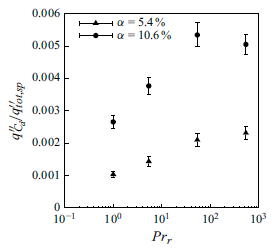


 Open access