2. Solver set-up and simulation parameters

Computations solve the three-dimensional compressible Navier–Stokes equations in generalized curvilinear coordinates using an implicit large-eddy simulation (LES) framework, using the formulation

(2.1)\begin{equation} \frac{\partial}{\partial \tau} \left(\frac{\boldsymbol{Q}}{J}\right) ={-}\left[\left(\frac{\partial \boldsymbol{F_i}}{\partial \xi} + \frac{\partial \boldsymbol{G_i}}{\partial \eta} + \frac{\partial \boldsymbol{H_i}}{\partial \zeta}\right) + \frac{1}{Re} \left(\frac{\partial \boldsymbol{F_v}}{\partial \xi} + \frac{\partial \boldsymbol{G_v}}{\partial \eta} + \frac{\partial \boldsymbol{H_v}}{\partial \zeta}\right)\right], \end{equation}

where $\boldsymbol {Q}=[\rho,\rho u,\rho v, \rho w, \rho E]^{\rm T}$ is the vector of conserved variables, where $\rho$ is the density, and $(u,v,w)$ are velocity components in Cartesian coordinates. The total specific internal energy is given by $E={T}/{[\gamma (\gamma -1){M_j}^2]}+(u^2+v^2+w^2)/2$, where $T$ is temperature, $\gamma$ is the ratio of the specific heats and ${M_j}=1.5$ is the reference jet Mach number at the nozzle exit. Here $J=\partial {(\xi,\eta,\zeta,\tau )}/\partial {(x,y,z,t)}$ is the Jacobian, $(\boldsymbol {F_i}, \boldsymbol {G_i}, \boldsymbol {H_i})$ denote the inviscid fluxes while $(\boldsymbol {F_v}, \boldsymbol {G_v}, \boldsymbol {H_v})$ denote the viscous fluxes, along the computational coordinates, ($\xi, \eta, \zeta$), respectively. The system of equations is closed using the ideal gas law, $p=\rho T/{\gamma {M_j}^2}$, while assuming a constant Prandtl number of $Pr=0.72$. Effects of temperature on viscosity are modelled using Sutherland's law. Further details of the formulation are available in Garmann (Reference Garmann2013).

In the following description starred quantities ($\{{\cdot }\}^*$) denote dimensional variables. All primitive variables except pressure are non-dimensionalized by their corresponding values at the jet exit. Here $p=p^{*}/\rho _j^{*}U_j^{*2}$ is defined as the non-dimensional pressure. Based on the equivalent diameter of the rectangular nozzle, ${D_{eq}^*}$, (further explained in the subsequent section), the Reynolds number is defined as $Re=\rho _j^{*}U_j^{*}D_{eq}^{*}/\mu _j^{*}$. Non-dimensional time is defined as $t=t^*/T_C^*$, where $T_C^*={D_{eq}^*}/{U_j^*}$ is the characteristic time scale. Non-dimensional frequency, commonly referred to as Strouhal number, is defined as $St=f^*D_{eq}^*/U_j^*$, where $f^*$ is the dimensional frequency in Hz.

Convective fluxes are reconstructed using a seventh-order weighted essentially non-oscillatory scheme (Liu, Osher & Chan Reference Liu, Osher and Chan1994) in the smooth regions of the flow. The Roe scheme (Roe Reference Roe1981) is then used to evaluate interface fluxes. Viscous fluxes are discretized using second-order central difference. Time integration is performed using a nonlinearly stable third-order Runge–Kutta scheme (Shu & Osher Reference Shu and Osher1988).

The orthogonal grid (shown in figure 1a) consists of ${\sim }47.53 \times 10^6$ nodes, and is discretized using $511$ nodes along the streamwise direction, and $309$ and $301$ nodes along the directions corresponding to the shorter and longer edges of the nozzle, respectively. Grid refinement is provided near the nozzle walls and exit, with a minimum wall-normal spacing, $\Delta n \sim 0.001$. Typical grid spacing in the plume is $\Delta x \sim 0.025$, while the transverse grid spacing near the shear layer is $\Delta y, \Delta z \sim 0.001$. Stretched grids near outflow boundaries minimize numerical reflections into the domain. The computational domain extends to ${\sim }30 D_{eq}$ in the streamwise direction and ${\sim }12 D_{eq}$ along the other two orthogonal directions. These parameters are informed by prior studies (Chakrabarti et al. Reference Chakrabarti, Gaitonde and Unnikrishnan2021) on supersonic rectangular jets at comparable $Re$. A grid convergence study is also performed to assess the effects of mesh resolution on the plume of the baseline jet by comparing results from a coarse and fine grid. Details of this study are summarized in the Appendix. Based on this, the following results are computed on the finer grid.

Figure 1.

(a) Principal planes of the computational domain and the boundary conditions utilized in the simulations. Every fourth node is shown. (b) Schematic of the nozzle and actuators. Nozzle and actuator dimensions, and principal planes are also shown.

The simulated flow fields correspond to a Mach $1.5$ (design Mach number) jet, exiting from a rectangular nozzle. The nozzle has an AR of $2:1$, with dimensions of $0.950$ inches (24.13 mm) along the longer edge and $0.475$ inches (12.06 mm) along the shorter edge (see figure 1b). These dimensions correspond to that reported in Isfahani, Webb & Samimy (Reference Isfahani, Webb and Samimy2021). The nozzle is modelled as a constant-area sleeve with a streamwise length, 3.67 equivalent diameters. The nozzle sleeve is visualized in figure 1(a). In this study the major axis plane is defined as the plane perpendicular to the shorter edges, and the minor axis plane as that perpendicular to the longer edges. The equivalent diameter of the rectangular jet is defined as $D_{eq}^* = \sqrt {(4/{\rm \pi} ) \times A_{exit}^*} = 0.758$ inches (19.25 mm). This is the equivalent diameter of a circular nozzle with an exit area the same as that of the rectangular nozzle. Based on the above reference quantities, $Re=\rho _j^{*}U_j^{*}D_{eq}^{*}/\mu _j^{*} \sim 1.09 \times 10^{6}$.

In the current study the Mach 1.5 jet is perfectly expanded and operates at a nozzle pressure ratio (ratio of stagnation pressure, $p_o^*$, to ambient pressure) of $3.67$. The exiting jet is unheated at a velocity $u^{*}_{jet} = 424.74\,{\rm m}\,{\rm s}^{-1}$ and static temperature $T^{*}_{jet} = 224\,{\rm K}$. The ambient pressure is $p_{\infty }^* = 101.325\,{\rm kPa}$ and the temperature is $T^{*}_{\infty } = 300\,{\rm K}$. The free-stream flow outside the nozzle imposes a small streamwise velocity of $u^{*}_{\infty }=0.01 \times u^{*}_{jet}$ in order to effectively implement characteristic boundary conditions. The boundary conditions are also detailed in figure 1(a). Characteristic boundary conditions (Poinsot & Lele Reference Poinsot and Lele1992; Blazek Reference Blazek2001) are imposed on all outer boundaries outside the nozzle. To minimize reflections, along with grid stretching, the order of reconstruction is also reduced locally near the outer boundaries. The nozzle surfaces are treated as no-slip adiabatic walls. On the inlet boundary within the nozzle block, the computations impose Dirichlet inflow conditions, similar to Bogey & Bailly (Reference Bogey and Bailly2010). Based on experimental estimates (Samimy et al. Reference Samimy, Kim, Kastner, Adamovich and Utkin2007a), the exiting boundary layers in these high-speed jets are around 1 mm in thickness. Therefore, velocity and density profiles corresponding to a boundary layer thickness $\delta _{99} \sim 0.85\,{\rm mm}$ are utilized. To aid development of stochastic perturbations in the shear layer, spatiotemporally correlated ‘coloured’ pressure perturbations are imposed on the boundary layer (Adler et al. Reference Adler, Gonzalez, Stack and Gaitonde2018), and is allowed to develop over the length of the nozzle sleeve before exiting into the ambient. This leads to a broadband spectra within the boundary layer and subsequently in the shear layer. A non-dimensional time step of ${\Delta t^*}/{T_C^*}=5 \times 10^{-4}$ is used for time integration. In all the simulations time-accurate data are obtained for 200 characteristic time intervals ($T_{C}^{*}$) at a sampling rate of $St=20$. This was found sufficient for convergence of first- and second-order statistics in the turbulent plume, and far-field acoustic predictions, which was verified using multiple sampling lengths of the data. The reported overall sound pressure level (OASPL) is calculated by integrating the power spectral density between $0.05 \le St \le 1.5$.

The LAFPA actuator is modelled as a surface heating condition, based on prior computational studies (Gaitonde & Samimy Reference Gaitonde and Samimy2011). Eight actuators are considered in this study, arranged around the nozzle inner wall close to the exit. Three actuators each are present along the longer edges of the nozzle, placed equidistant from the walls as well as each other (see figure 1b). One actuator each is present at the centre along the two shorter edges of the rectangle. Each actuator surface has dimensions of $0.1'' (2.5\,{\rm mm}) \times 0.03'' (0.75\,{\rm mm})$ ($l \times b$). The centre of each actuator is located $0.0569'' (1.44\,{\rm mm})$ from the nozzle exit. These are based on corresponding LAFPA model dimensions tested on circular jets (Gaitonde Reference Gaitonde2012). When the actuator is on, the local surface temperature increases to $T=5 T_{\infty }$, which is informed by spectroscopic temperature measurements from experiments (Samimy et al. Reference Samimy, Kim and Kearney-Fischer2009; Gaitonde & Samimy Reference Gaitonde and Samimy2010).

In the present study, in addition to the baseline case, we evaluate five types of actuation involving various spectral and duty cycle combinations, which are some of the most significant parameters affecting the response of the jet. These are tabulated in table 1. The choice of these parameters are influenced by their significance identified in the previously mentioned LAFPA-based experiments. While $St=0.3$ allows us to study the forced response to the most sensitive input near the column mode of the jet, $St=1$ is representative of an effective frequency range for LAFPA control. Here $St=2$ will provide insights on the shear layer response to relatively higher frequencies outside the dominant shear layer spectrum. Figure 2 plots the temperature signature of the actuators in the above cases. The abscissa is non-dimensional time, $t$, and the ordinate is normalized temperature ($T/T_{\infty }$). Forcing frequency specifies the number of actuation cycles per unit non-dimensional time, while the duty cycle determines the duration within an actuation cycle over which the actuator is on. For example, a frequency of $St=2$ has the actuator switching on and off twice per unit non-dimensional time, and a duty cycle of $50\,\%$ indicates that the actuator is switched on for $50\,\%$ of each cycle. To simplify the parameter space, we limit the evaluation to ‘axisymmetric’ excitation, where all eight actuators operate in identical phase. For notational convenience, in the following the duty cycle will be referred to as ‘DCX’, where ‘X’ refers to the duty cycle percentage. It has to be noted that for $St=0.3$ forcing, only a single duty cycle is tested, since it results in significant increases in far-field noise levels due to the amplification of the column mode in the jet plume.

Figure 2.

Temporal variation of imposed excitation for cases shown in table 1; (a–c) $20\,\%$ duty cycle and (d,e) $50\,\%$ duty cycle.

Table 1.

Forcing frequencies and duty cycles.

3. Baseline characteristics and validation

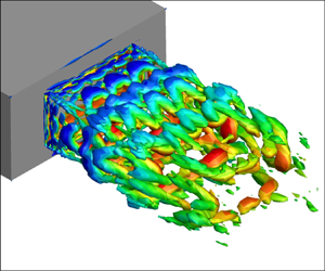
The flow field of the baseline jet is visualized in figure 3. It highlights vortical structures in the turbulent plume using an isolevel of Q criterion, coloured by streamwise velocity ($u$). Close to the nozzle exit, thin spanwise roller vortices are evident that experience a higher convective velocity along the inner shear layer region, as depicted by the colouring. As the shear layer spreads, these spanwise vortices transform into horse-shoe vortices that dominate the plume, until about the core collapse location. Further downstream, streamwise elongated vortex tubes are predominant. Turbulent mixing eventually leads to disintegration of coherent vortices into smaller scale structures.

Figure 3.

Instantaneous snapshot of the baseline jet. Vortical features are highlighted using isolevels of the Q criterion, coloured by streamwise velocity.

We now validate the baseline simulation using published data on mean flow-field parameters and acoustic signature of the jet. The centreline mean velocity is plotted in figure 4(a) for jets operating under comparable conditions. The current result is denoted ‘current study’ and is compared with computational data of a Mach $1.5$, ${\rm AR}=2:1$ rectangular jet, available in Viswanath et al. (Reference Viswanath, Johnson, Corrigan, Kailasanath, Mora Sanchez, Baier and Gutmark2016), and that from simulations of an ${\rm AR}=3:1$ rectangular jet, reported in Seror et al. (Reference Seror, Sagaut, Bailly and Juvé2000). In addition, experimental data of an ${\rm AR}=3:1$ rectangular jet compiled by Kinzie (Reference Kinzie1995) are also included. While the ${\rm AR}=2:1$ is a non-method-of-characteristics (MOC) convergent-divergent (CD) nozzle, the latter CD nozzles (with ${\rm AR}=3:1$) have diverging sections designed using MOC, and are hence chosen for comparison. The current computations show a relatively closer match with the experimental data and computations by Seror et al. (Reference Seror, Sagaut, Bailly and Juvé2000) for the ${\rm AR}=3:1$ rectangular nozzle. The core collapse location ($x \sim 5.8$) and rate of velocity decay due to entrainment also compare well with the above data. Weak oscillations of the centreline velocity in the current study is due to a slight pressure mismatch between the ambient and nozzle flow, resulting from the flow development within the nozzle block. The difference in current computations and that of Viswanath et al. (Reference Viswanath, Johnson, Corrigan, Kailasanath, Mora Sanchez, Baier and Gutmark2016) is due to the presence of shock-expansion cells induced by the non-MOC design of the nozzle diverging section in the latter. Comparisons with circular jets at similar operating conditions (not included in the figure) also indicated that the rate of collapse of the potential core is higher in the rectangular jet when compared with a circular jet operating at similar conditions, consistent with prior studies (Chakrabarti et al. Reference Chakrabarti, Gaitonde and Unnikrishnan2021). This is due to the relative proximity of shear layers developing along the longer edges of the nozzle (i.e. shear layers visible on the minor axis plane in the current convention).

Figure 4.

(a) Centreline velocity comparison. (b) Spreading-rate comparison on minor axis plane.

To quantify the spreading rate of the jet, we utilize the transverse location where the mean streamwise Mach number ($\overline {M_x}$) attains a value, $\overline {M_x}=0.2$, following the convention in Viswanath et al. (Reference Viswanath, Johnson, Corrigan, Kailasanath, Mora Sanchez, Baier and Gutmark2016). This is plotted as $h_{0.2}$ in figure 4(b), on the two principal planes, for the current study and computations by Viswanath et al. (Reference Viswanath, Johnson, Corrigan, Kailasanath, Mora Sanchez, Baier and Gutmark2016). A reasonable match is observed on the minor axis plane between the two. The variation on the major axis plane is primarily due to the delayed initiation of spreading of the shear layer in the reference calculation, which can be attributed to the shock train at the nozzle exit. However, downstream of $x \sim 2$, the spreading rate is comparable between the two computations, as suggested by the two curves being almost parallel to each other.

The far-field signature of the baseline jet obtained from the acoustic field is shown at a location of $r=40$ on the minor axis plane in figure 5. The far-field acoustic signature is obtained by first performing an acoustic filtering (Unnikrishnan & Gaitonde Reference Unnikrishnan and Gaitonde2016), as detailed in § 5.2. The filtered acoustic fluctuations from a cylindrical surface at $r=2.5$ are then propagated into the far field using a time-domain linear wave propagator. Details about the associated theory, implementation and validation have been published by Unnikrishnan, Cavalieri & Gaitonde (Reference Unnikrishnan, Cavalieri and Gaitonde2019). For spectral calculations, the minimum bin is $St=0.01$, and the Welch method (Welch Reference Welch1967) is utilized with the signal segmented into five windows with $75\,\%$ overlap, consisting of 2048 points. This is compared with microphone data from experiments at the University of Cincinnati, and the corresponding computations, reported in Viswanath et al. (Reference Viswanath, Johnson, Corrigan, Kailasanath, Mora Sanchez, Baier and Gutmark2016). Figure 5(a) shows the sound pressure level (SPL) comparison at a polar angle of $\theta = 36^{\circ }$, measured from the jet downstream direction, and roughly corresponds to the direction of peak radiation of the jet. The acoustic spectra of the current study matches very well with experimental data and lies in between the upper and lower envelopes of the spectral predictions from the reference computations. As expected from a perfectly expanded jet, the noise spectra is mostly broadband, with relatively lower energy at higher frequencies. There exists a broadband energy peak at low-to-mid band frequencies between $0.2 \le St \le 0.4$ ($4.4\,{\rm kHz} \le f \le 8.8\,{\rm kHz}$), corresponding to the column mode of the jet. This trend is consistent with the universal F-spectrum mixing noise curve identified by Tam, Golebiowski & Seiner (Reference Tam, Golebiowski and Seiner1996). Figure 5(b) shows the SPL comparison at a polar angle of $\theta = 80^{\circ }$, which is along the jet sideline. There is a good match at higher frequencies, and some over-prediction at lower frequencies. This may be attributed to the differences in characteristics of fine-scale turbulence (Tam, Pastouchenko & Viswanathan Reference Tam, Pastouchenko and Viswanathan2005; Tam Reference Tam2019) of the jet shear layers between the current study and reference studies, which is caused by the dissimilarities in the boundary layer characteristics exiting the nozzle (Brès et al. Reference Brès, Jordan, Jaunet, Le Rallic, Cavalieri, Towne, Lele, Colonius and Schmidt2018). The flat broadband spectral shape is also consistent with the G-spectrum mixing noise curve proposed by Tam et al. (Reference Tam, Golebiowski and Seiner1996).

Figure 5.

Far-field SPL comparison at polar angles of (a) $36^{\circ }$ and (b) $80^{\circ }$ on the minor axis plane.

4. Acoustic impact of control

Since noise mitigation is a major consideration in LAFPA-based control of jets, we first detail the near-field and far-field acoustic impact of control. As discussed in § 2, the parameters considered here are the frequency and duty cycle of excitation.

4.1. Effect of forcing frequency

Depending on the forcing frequency, the jet may respond by energizing the large-scale coherent structures resulting in noise amplification, or reducing peak noise levels by redistribution of acoustic energy to off-peak frequencies or non-radiating wave speeds. To isolate the effect of forcing frequency, the duty cycle is fixed at $20\,\%$ (DC20) in this section, where we first describe the near-field trends in the LES domain, followed by the far-field acoustic signature.

4.1.1. Near-field impact

The phase-averaged acoustic near-field is presented in figure 6 using contours of dilatation ($\boldsymbol {\nabla } \boldsymbol {\cdot } \boldsymbol {u}$) for the baseline and controlled cases. Phase averaging on the controlled cases is performed by considering one cycle of the respective forcing frequency to be the reference signal. Since the baseline jet has no associated unique forcing signal, phase averaging is performed at all three frequencies ($St=0.3, 1$ and $St=2$) in order to compare with the controlled cases. The first snapshot obtained after attaining statistical stationarity of the simulation is considered as the beginning of the phase cycle in the baseline case.

Figure 6.

Phase-averaged dilatation contours of baseline (upper) and controlled (lower) cases corresponding to $St=0.3$ on the (a) major axis plane and (b) minor axis plane. Corresponding results for (c,d) $St=1$ forcing and (e, f) $St=2$ forcing.

The results presented correspond to a phase of ${\rm \pi}$ within each phase-averaged cycle. Bottom panels in figure 6(a,c,e) show phase-averaged dilatation contours on the major axis plane of the jet, corresponding to forcing at $St=0.3, 1$ and $St=2$, respectively. The same is shown for the minor axis plane in figure 6(b,d, f). The upper panel in each subfigure is the baseline jet phase averaged at the corresponding frequency.

Dilatation contours of the baseline jet phase averaged at $St=0.3$ (figure 6a,b) show strong directive acoustic radiation at an angle of $\theta \sim 30^{\circ }$, which roughly corresponds to the angle at which peak OASPL (${\sim }129$ dB) is observed on both principal planes, consistent with experiments of Heeb et al. (Reference Heeb, Mora Sanchez, Gutmark and Kailasanath2013). The directivity of this radiating stream is highlighted by a red line segment. Since the column mode of the jet exists in the spectral vicinity of $St=0.3$ (Crow & Champagne Reference Crow and Champagne1971; Kibens Reference Kibens1980; Petersen & Samet Reference Petersen and Samet1988), this forcing produces the strongest response from the jet, as also seen in experiments by Samimy et al. (Reference Samimy, Kim, Kastner, Adamovich and Utkin2007a). Here $St=0.3$ forcing causes the naturally occurring directional radiation to intensify, leading to a significant increase in peak OASPL at $\theta \sim 34^{\circ }$, and also elevated noise levels across polar angles. The acoustic waves have a periodic fish bone pattern similar to that observed by Gaitonde (Reference Gaitonde2012) in their simulations of axisymmetric jets. The intensity of acoustic waves generated by forcing at $St=0.3$ is higher on the minor axis plane than on the major axis plane. Comparison of the root-mean-square (RMS) pressure fluctuations at a distance of $y/z=2.5$ from the nozzle lip line on the two principal planes showed that, along shallow angles measured with respect to the jet lip line $(\theta \sim 25^{\circ })$, the pressure fluctuations on the minor axis plane were up to $22\,\%$ higher than that on the major axis plane.

The phase-averaged dilatation field of the baseline jet with $St=1$ as the reference signal (figure 6c,d) shows very weak acoustic radiation, consistent with the roll-off in acoustic energy at higher frequencies. The controlled jet responds to forcing at this frequency by producing two dominant streams of acoustic radiation on the minor axis plane. The first stream is predominantly downstream, eventually spreading across the plane of propagation within $20^{\circ } \le \theta \le 60^{\circ }$. As a consequence, the downstream direction experiences additional radiation that was not present in the baseline case. This is induced by intrusion of vortical structures into the potential core, as shown in the phase-averaged flow field in figure 7(a).

Figure 7.

Phase-averaged vorticity and corresponding dilatation contours at a phase of ${\rm \pi}$ in the near nozzle regions for (a) $St=1$ and (b) $St=2$ actuation on the minor axis plane. The blue dot in (a) represents the point where the time trace of acoustic fluctuations (${-\partial \psi _{a}'}/{\partial x}$) are extracted, while the dashed blue line represents the series of spatial locations over which the time trace of vorticity fluctuations ($\omega _{z}'$) are extracted. The dashed blue line in (b) represents the location where $x$-$t$ variation of vorticity fluctuations ($\omega _{z}'$) are studied. Potential core outlines using the $u=0.9$ contour, represented by the pink solid line.

Energy dynamics of such intrusion events and associated acoustic radiation have been detailed in Unnikrishnan & Gaitonde (Reference Unnikrishnan and Gaitonde2016). This is further analysed using the cross-correlation of acoustic fluctuations (${-\partial \psi _{a}'}/{\partial x}$) (Unnikrishnan & Gaitonde Reference Unnikrishnan and Gaitonde2016) and vorticity fluctuations ($\omega _{z}'$). Acoustic fluctuations are obtained at $x=3.7$ from the nozzle exit, and $y=2.5$ from the centreline, corresponding to a polar angle of $\theta \sim 34^{\circ }$, and is denoted by a blue dot in figure 7(a). Vorticity fluctuations are obtained along a horizontal line, $y=0.2$, from the centreline. Figure 8(a) shows the cross-correlation contours where the abscissa represents the distance from the nozzle exit and the ordinate represents a non-dimensional time lag. Correlation peaks exist in $1 \le x \le 2.5$, with peak values at $x \sim 1.5$, which is the location where vortex intrusion is identified in figure 7(a). This indicates that vorticity fluctuations (due to vortex intrusion) at these spatial locations are closely associated with acoustic fluctuations in the downstream radiating direction. From the perspective of shear layer instability waves, this response to forcing can also be interpreted as the enhancement of the Kelvin–Helmholtz instability wave packet at the forcing frequency, resulting in increased downstream radiation (Cavalieri, Jordan & Lesshafft Reference Cavalieri, Jordan and Lesshafft2019).

Figure 8.

(a) Cross-correlation contour for $St=1$ forcing, and (b) wavenumber-frequency contour for $St=2$ forcing.

The second stream of acoustic radiation seen in figure 6(c,d) is predominantly in the sideline direction ($70^{\circ } \le \theta \le 90^{\circ }$). This emerges from the nozzle exit and, therefore, is most likely a direct signature of the perturbations emitted from the plasma actuator. The behaviour of the first (downstream) acoustic stream is similar on both the principal axes, whereas the spatial form of the second (sideline) stream differs on these two planes. This reaffirms the hypothesis that the sideline band is a direct signature of actuation, which is more likely to be affected by the variations in actuator placement on the longer and shorter edges of the nozzle. Although not discernible from figure 6(c,d) due to its relatively low-amplitude sideline signature, the $St=1$ forcing results in a feeble interference pattern between the above two streams.

A similar analysis on the baseline jet phase averaged with $St=2$ as the reference signal indicates a negligible presence of high frequencies in the near field (figure 6e, f). The controlled jet, however, reveals a response pattern containing three dominant acoustic streams on the minor axis plane. The first has a predominantly downstream directivity pattern, with $\theta \le 50^{\circ }$, as seen in figure 7(b). This can be attributed to the supersonic convection of coherent vortical waves in the thin shear layer. To probe this further, we obtain the space–time Fourier-transformed vorticity fluctuations ($\omega _{z}'$) along the nozzle lip line (represented by a dotted blue line in figure 7b). The wavenumber–frequency contour plot is shown in figure 8(b). The abscissa represents wavenumber ($k$), the ordinate represents frequency ($St$) and the contours correspond to the logarithm of energy. Only the regime of positive wavenumbers are shown, as the contribution to energy from upstream propagating waves is significantly lower than that of the downstream propagating waves. The ratio of the abscissa to ordinate yields the convective speed $St/k$, which is equivalent to ($1/2{\rm \pi}$)$\omega /k$. The blue dotted line, red dashed line and green dashed-dot line on these contours represent phase speeds of $u-c$, $c$ and $u+c$, respectively. Here, $c$ is the speed of sound based on jet exit conditions and $u$ is the jet exit velocity. Thus, any energy content to the left of the red dashed line has a locally supersonic convective speed and contributes towards acoustic emissions. In figure 8(b) almost half of the energetic spectral range appears in the supersonic regime. As suggested by the low wavenumbers, it is evident that coherent vortical structures travelling at locally supersonic convective speed are responsible for the emission of Mach waves in the downstream direction.

The second stream of acoustic waves in figure 6(e, f) is along the sideline direction, representative of the actuator signature, with much higher intensity than that observed for the $St=1$ forcing. The asymmetry of this stream on the two planes can again be associated to the difference in the number actuators placed on the longer and shorter edges of the nozzle. The third stream with peak radiation along $\theta = 60^{\circ }$ appears to be a result of interaction between the downstream radiation and the sideline actuator signature. A similar three-stream pattern is seen on the major axis plane, albeit at lower amplitudes.

4.1.2. Far-field impact

The far-field acoustic impact of forcing is quantified in figure 9 by plotting the polar variation of far-field OASPLs on the two principal planes of the nozzle at $r=40$. Figure 9(a,c) shows variation of the OASPL, and figure 9(b,d) shows the change in OASPL levels of the controlled jets in relation to the baseline jet. This is calculated using

(4.1)\begin{equation} \Delta {\rm OASPL} = {\rm OASPL}_{Controlled}- {\rm OASPL}_{Baseline}. \end{equation}

Negative/positive values of $\Delta {\rm OASPL}$ signify noise reduction/increase upon implementing control. The sound levels of the baseline jet are nearly identical on the major and minor axis planes, consistent with the azimuthally axisymmetric far-field acoustics seen in low-AR rectangular jets without flapping (Heeb et al. Reference Heeb, Mora Sanchez, Gutmark and Kailasanath2013; Viswanath et al. Reference Viswanath, Johnson, Corrigan, Kailasanath, Mora Sanchez, Baier and Gutmark2016; Chakrabarti et al. Reference Chakrabarti, Gaitonde and Unnikrishnan2021). However, the impact of control is different on the two planes.

Figure 9.

Far-field OASPL comparison between the baseline jet and jets with control at various polar angles on (a) the major axis and (c) the minor axis plane. The OASPL difference between the baseline jet and jets with control at the same far-field locations on (b) the major axis and (d) the minor axis plane. Red horizontal lines in (b,d) indicate the 0 dB datum.

When the jet is forced at $St=0.3$, the noise levels across polar angles increase significantly. The increase in peak noise levels is about 5 dB on the minor axis plane, and slightly over 3 dB on the major axis plane, as seen in the $\Delta {\rm OASPL}$ levels. The acoustic asymmetry is more prominent at shallow polar angles, with the sideline angles indicating comparable $\Delta {\rm OASPL}$ levels on both the planes. The asymmetry could be contributed by the inherent differences between the nature of coherent structures excited in the shear layers, as well as differences in the number of actuators between the shorter and longer edges of the nozzle. The nature of the excited shear layer structures on the two planes will be further explored in the following section using phase-averaged analysis. Recent linear analysis by Rodriguez, Prasad & Gaitonde (Reference Rodriguez, Prasad and Gaitonde2021) has identified an elliptic nature to wave packets in rectangular jets. Upon excitation, energizing of these wave packets can also contribute to enhanced asymmetry in the associated radiation pattern. This asymmetric noise amplification is consistent with increased intensity of super-directive acoustic waves seen in the phase-averaged dilatation contours (figure 6a,b).

High-frequency forcing (at $St=1\ {\rm and}\ 2$) causes the far-field OASPL to reduce at certain polar angles, typically $\theta \le 40^{\circ }$, as seen in figure 9. Noise attenuation is also different between the two planes, with maximum reduction obtained on the major axis plane. On the major axis plane, forcing at $St=1$ provides ${\sim }1$ dB reduction at angles of peak noise levels ($20^{\circ } \le \theta \le 40^{\circ }$). The sideline also shows reduced noise levels that is consistent with the observation that the phase-averaged acoustic radiation signature on the major axis plane is significantly weaker in relation to the minor axis plane (figure 6c,d). The effectiveness of $St=1$ forcing on the minor axis plane is relatively weaker. While noise levels at very-low polar angles indicate reduction, the peak noise levels remain similar to that in the baseline jet. The increase in noise levels at $\theta > 70^{\circ }$ results from the additional sideline radiation seen earlier in the phase-averaged contours.

Forcing at $St=2$ also has different signatures on the two planes, but sound reduction achieved at peak noise polar angles is relatively smaller. On the minor axis plane, the peak reduction is at $\theta = 45^{\circ }$. A lack of noise reduction along downstream angles, $\theta \le 40^{\circ }$, is attributed to the first stream of acoustic radiation seen earlier in figure 6( f). A similar loss in control effectiveness is observed at $\theta \sim 60^{\circ }$, owing to the third stream of acoustic waves. The marginal noise increase at $\theta > 75^{\circ }$ is due to the additional sideline radiation emerging as a result of actuation. Main differences on the major axis plane are that the peak noise reduction is higher (by ${\sim }0.5$ dB), and the sideline noise also attenuates. Both these can be attributed to the fact that the acoustic waves from actuation on the major axis plane are of lower intensity than the minor axis plane.

The trends observed in $\Delta {\rm OASPL}$ are further explored using the SPL spectra in figure 10. The SPL at $\theta =34^{\circ }$, corresponding to the polar angle of peak radiation, are shown in figure 10(a,c), for the major and minor axis planes, respectively. Corresponding SPL plots at $\theta =80^{\circ }$ (jet sideline) are shown in figure 10(b,d). Each plot contains the baseline and controlled jets. The actuator signature appears as sharp peaks at forcing frequencies in the spectra. A key observation is that the actuator signature is much stronger (higher amplitude peaks) on the minor axis plane than on the major axis plane, consistent with the observations made in near-field phase-averaged contours.

Figure 10.

Effects of forcing frequency on far-field SPL: comparison of results form the baseline jet and jets with control at a peak noise radiating angle of $\theta = 34^{\circ }$ on (a) the major axis and (c) the minor axis. Plots (b,d) are corresponding results at a jet sideline angle of $\theta = 80^{\circ }$.

Forcing at $St=0.3$ generates the most dominant peak over the broadband hump (of the baseline), with a magnitude that is 3 to 5 dB higher, contributing to the increased OASPL seen earlier in figure 9. The jet sideline, however, does not experience such a drastic increase in sound levels, confirming the observation that the impact of $St=0.3$ forcing is primarily to increase the super-directive radiation. These observations regarding the sideline also match with experimental results by Samimy et al. (Reference Samimy, Kim and Kearney-Fischer2009) for LAFPA-controlled circular jets, where OASPL in the sideline did not show any appreciable change.

Forcing at $St=1$ decreases the radiated energy, particularly at low- and mid-band frequencies in comparison to the baseline case. The encouraging observation is that, at peak radiating angles, energy within the broadband hump ($0.2 \le St \le 0.4$) corresponding to the jet column mode is reduced. For peak radiating angles, the actuator signature is much smaller on the major axis plane, with a magnitude lower than the broadband noise hump. This explains the higher levels of noise attenuation on the major axis plane (figure 9). Along the jet sideline, forcing at $St=1$ induces very little variations in the energy content at most frequencies. This coupled with the additional signature of the actuators result in an increase in sideline OASPL.

Forcing at $St=2$ has minimal favourable impact on the radiated energy, with noise reduction limited to higher frequencies ($St > 0.6$). However, $St=2$ has a relatively weaker far-field actuator signature compared with the other cases.

A similar trend of noise reduction was observed with a higher duty cycle of $50\,\%$, with forcing frequencies of $St=1$ and $St=2$. In summary, among the various frequencies of actuation studied, $St=1$ forcing yields a good balance between reduced overall sound levels and moderate increase in sideline noise levels on some nozzle planes. This must also be interpreted in the context that the sideline noise levels are much lower (by ${\sim }12$ dB) than the peak noise levels.

4.2. Effect of duty cycle

Since forcing at $St=1$ was observed to be the most effective in the previous analysis, we report the impact of the duty cycle at this frequency. Studies by Speth & Gaitonde (Reference Speth and Gaitonde2013) on circular jets showed that while the plume response was sensitive to lower duty cycles, higher duty cycles typically above $50\,\%$ showed very similar mean flow and fluctuation statistics. They also reported that a jet forced at a $100\,\%$ duty cycle had a behaviour that closely resembled an uncontrolled jet. Based on these observations, the present study is limited to two duty cycles, $20\,\%$ and $50\,\%$. The results are presented in figure 11 for DC20 and DC50. Figure 11(a,c) shows the far-field OASPL comparison among the baseline and the two controlled jets on the major and minor axis planes, respectively. Figure 11(b,d) shows the corresponding $\Delta {\rm OASPL}$.

Figure 11.

Effects of duty cycle on far-field noise: far-field OASPL comparison between the baseline jet and jets with $St=1$ DC20/DC50 control at various polar angles on (a) the major axis and (c) the minor axis plane. Corresponding OASPL differences between controlled jets and the baseline jet on (b) the major axis and (d) the minor axis plane. Red horizontal lines in (b,d) indicate the 0 dB datum.

Comparing figures 11(b) and 11(d), the major axis shows higher levels of noise attenuation for both duty cycles. Although both DC20 and DC50 attain ${\sim }1.3$ dB reduction for shallow angles ($10^{\circ } \le \theta \le 30^{\circ }$), the latter outperforms along peak noise angles corresponding to $\theta \sim 35^{\circ }$. This is evident in figure 11(b), where the maximum reduction is obtained as 1.6 dB for DC50. The higher duty cycle also reduces the $\Delta {\rm OASPL}$ overshoot at $\theta \sim 55^{\circ }$, further improving the overall performance. Although not as effective as on the major axis plane, DC50 still performs better than DC20 on the minor axis plane. As opposed to the major axis trends, the noise in the controlled jets increases along the sideline ($\theta > 75^{\circ }$) on the minor axis plane, due to the direct response to the forcing frequency, which causes increased sideline radiation as discussed in the previous section.

Figure 12 shows the SPL spectra comparison among the baseline and controlled cases. The left and right columns correspond to $\theta =34^{\circ }$ and $\theta =80^{\circ }$, respectively. The top and bottom rows correspond to major and minor axis planes, respectively. The improved performance of DC50 on the major axis plane is due to the SPL reduction near the column mode frequency, $0.2 \le St \le 0.4$, and higher frequencies, $0.6 \le St \le 0.7$. This, along with the relatively weaker actuation signature facilitates the 1.6 dB reduction in overall noise levels seen earlier in figure 11(b). A similar reduction in SPL is seen on the minor axis plane as well in figure 12(c), but the reduction at column mode frequency is not as much as that seen on the major axis plane. On both the major and minor axis planes, neither duty cycles impact the sideline spectra significantly, as seen in figure 12(b,d). Therefore, the emergence of the actuator tone effectively increases the OASPL.

Figure 12.

Effects of duty cycle on far-field noise: far-field SPL comparison between the baseline jet and jets with control at a peak noise radiating angle of $\theta = 34^{\circ }$ on (a) the major axis and (c) the minor axis. Plots (b,d) are the corresponding results at a jet sideline angle of $\theta = 80^{\circ }$.

The foregoing analyses confirm that the forcing at $St=1$ with a $50\,\%$ duty cycle provides the most reduction in far-field sound, within the parameter space tested. They also highlight the fact that the choice of forcing frequency plays a crucial role in altering noise characteristics of the jet, due to its manipulation of shear layer instabilities and evolution of coherent structures. The duty cycle seems to provide a secondary effect by reinforcing this response. As highlighted in § 1, a key focus of this study is to identify causal mechanisms in the plume that directly result in the observed acoustic trends. To this end, the following sections will first explore in detail the shear layer dynamics and radiating characteristics of key controlled cases. This will be followed by evaluation of first- and second-order turbulent statistics of these jets.

5. Response of the plume to actuation

Dynamics of the forcing frequency in the plume has a major impact on the resulting spatiotemporal scales in the controlled jets. While coherent turbulent features in the response may be highlighted through a vortex-identification technique, its acoustic impact can be identified using a suitable physical filtering strategy (Tinney & Jordan Reference Tinney and Jordan2008; Unnikrishnan & Gaitonde Reference Unnikrishnan and Gaitonde2016). These will be utilized below in conjunction with the phase-averaged flow field to study the controlled jets.

5.1. Shear layer response

The response of the shear layer to actuation is evaluated in figure 13(a–c) for $St=0.3$, $St=1$ and $St=2$ forcings, respectively, at a $50\,\%$ duty cycle, using a phase-averaged Q criterion ($\tilde {Q}$), coloured with phase-averaged streamwise velocity ($\tilde {u}$). The four snapshots, figure 13(a–d), correspond to the states at four representative time instances within the phase-averaged cycle, $0 \le \tilde {t} \le T_{f}$, in terms of the percentage of $\tilde {t}/T_{f}$. The time period of forcing, $T_{f}$, is defined as $1/St_{f}$, where $St_{f}$ is the non-dimensional frequency of forcing. To highlight the vortical dynamics, figure 13 identifies two flow structures, A1 and B1, at the beginning of the phase-averaged cycle in each case. Here A1 corresponds to the features that are generated when the actuators turn off, and eventually develop into lambda vortices; B1 is an elongated vortical element parallel to the shear layer, that is generated when the actuators turn on, at the beginning of a cycle. In each frame, the upper and lower arrows track A1 and B1, respectively.

Figure 13.

Phase-averaged flow fields for (a) $St=0.3$ (DC20), (b) $St=1$ (DC50) and (c) $St=2$ (DC50) forcing, at the indicated phase percentages. The top (B1) and bottom (A1) pointing arrows track the evolution of structures generated when the actuator is switched on and off, respectively. Distance between two vertical grid lines is 0.5$D_{eq}$.

With $St=0.3$ forcing (figure 13a), A1 and B1 flow structures convect downstream and the ‘legs’ of the A1 lambda vortices are stretched in the high-speed core, while the ‘head’ region lags in the ambient fluid as seen in figure 13(a-ii). Interaction of A1 with B1 vortical structures causes the head region to be pinched off, as seen in figure 13(a-iii,iv). The pinched head regions develop into a larger set of lambda vortices as shown by the dashed circle in figure 13(a-i). These vortices eventually coalesce to form a single lambda vortex that convects downstream as demarcated by the dashed circle in figure 13(a-ii,iii). This shows that the shear layer responds to the forcing at $St=0.3$ by generating large coherent vortical structures, at the scales of the plume, resulting in increased far-field noise levels.

For $St=1$ forcing, the initial development of A1 and B1 structures follow a similar pattern. The ‘legs’ of the A1 lambda vortices are stretched in the high-speed core, while the ‘head’ region lags in the ambient fluid, resulting in the head region being pinched-off from the vortical structure, as seen in figure 13(b-ii). However, further evolution of these vortical structures differ from the $St=0.3$ forcing. In figure 13(b-iii) the pinched head regions interact with the trailing vortical element, B1, and creates an ‘azimuthally’ connected vortical element. This results in a staggered pattern of lambda vortices in B1, relative to A1, evident in figure 13(b-iv). Comparing the velocity contours on A1 and B1 in figure 13(b-iv), B1 lambda vortices exist in the inner shear layer. Around $x \sim 2.5$ downstream of the nozzle exit, these structures disintegrate. Thus, $St=1$ forcing generates a flow response at the scales of the shear layer thickness, including streamwise vortices in the shear layer, generally considered favourable to reducing coherent sound generation mechanisms.

A similar analysis for $St=2$ forcing is shown in figure 13(c). The B1 vortex element initially parallel to the shear layer disintegrates downstream as seen in figure 13(c-ii), and merges with A1 to form a single row of lambda vortices. While the ‘head’ regions of this row of lambda vortices are formed by the A1 row of vortices present in the (low-speed) outer shear layer, the ‘legs’ are formed by the stretched B1 row of vortices that reside within the (high-speed) inner shear layer. These vortex rings are sustained to about $x \sim 1.5$ from the nozzle exit, after which they disintegrate. Unlike $St=1$ forcing, due to the rapid decay rate over a very small streamwise extent, and smaller spatial scales being impacted, $St=2$ forcing does not efficiently manipulate the energy-containing scales in the shear layer and, thus, only minimally affects the acoustic emissions.

5.2. Acoustic response of the plume

In the turbulent plume the fluctuations are dominated by the hydrodynamic content. Therefore, to understand the origin of the far-field noise signature of the controlled jets, we first isolate the acoustically relevant fluctuations in the plume using the following momentum potential theory (Doak Reference Doak1989):

(5.1)\begin{equation} \rho \boldsymbol{u} = \boldsymbol{\bar{B}} + \boldsymbol{B'} - \boldsymbol{\nabla} (\psi_{a}' + \psi_{T}'). \end{equation}

This is achieved by performing a Helmholtz decomposition of the mass flux. Here, $\bar {B}$ and $B'$ are the mean and fluctuating solenoidal components, respectively. The irrotational scalar potentials account for the acoustic ($\psi _{a}'$) and thermal ($\psi _{T}'$) components. Upon substituting the above relation in the continuity equation, we obtain two Poisson equations, which can be solved to extract the acoustic and thermal components in the jet, i.e.

(5.2a,b)\begin{equation} \nabla^2 \psi_a = \frac{1}{c^2}\frac{\partial p}{\partial t},\quad \nabla^2 \psi_T = \frac{\partial \rho}{\partial S}\frac{\partial S}{\partial t}. \end{equation}

Here $c$ is the local speed of sound and $S$ is entropy. More details on the decomposition and its implementation can be found in Unnikrishnan & Gaitonde (Reference Unnikrishnan and Gaitonde2016). The following discussion will focus on trends in the streamwise acoustic fluctuations, $(- {\partial \psi _{a}'}/{\partial x})$, due to its most influential role in defining the radiated noise in the downstream direction. It will be henceforth referred to as $A_{x}$ for notational convenience.

The effect of actuation on the acoustic component is first isolated from the phase locked averaging as specified in § 4.1. Figure 14 shows an instantaneous snapshot of phase-averaged acoustic fluctuations, $A_{x}$. The figure shows a plane projected view of the isolevels of $A_{x} = \pm 0.003$ for $St=0.3$, DC20 forcing (figure 14a,b) and $St=1$, DC50 forcing (figure 14c,d).

Figure 14.

Instantaneous isolevels of phase-averaged acoustic fluctuations at $A_{x} = \pm 0.003$ for $St=0.3$ DC20 forcing, projected onto (a) the major axis plane and (b) the minor axis plane. Plots (c,d) are corresponding results for the $St=1$ DC50 forcing. The potential core is shown using and isolevel at $u=0.9$. The distance between consecutive vertical and horizontal grid lines are 2$D_{eq}$ and 1$D_{eq}$, respectively.

In case of $St=0.3$ forcing the acoustic response is amplified into a mostly axisymmetric large-scale wave packet that extends beyond the potential core of the jet. This is due to the jet resonating at the column mode, thus developing a global response at the forcing frequency. As expected in radiatively efficient wave packets, the length scales of these features are significantly higher than the local turbulent scales (Cavalieri et al. Reference Cavalieri, Jordan, Colonius and Gervais2012). The response to $St=1$ forcing is an axially compact wave packet, largely limited to the vicinity of the nozzle. It exhibits a strong influence of the rectangular nozzle geometry, due to the non-axisymmetric nature of the mean flow. The direct spectral impact of the high-frequency actuation is thus local in nature, and mostly appears in the sideline direction.

6. Impact on radiating characteristics

From the previous analyses, it is evident that the acoustic response in the plume and its far-field signature are sensitive to control parameters. Here we examine three main characteristics of the acoustic gain of the jet, which helps us explain the observed noise signatures. Those include the convective speed of the acoustic wave packet (Tam & Morris Reference Tam and Morris1980; Tam & Burton Reference Tam and Burton1984a,Reference Tam and Burtonb), its azimuthal coherence (Sinha et al. Reference Sinha, Rodríguez, Brès and Colonius2014; Chakrabarti et al. Reference Chakrabarti, Gaitonde and Unnikrishnan2021) and intermittency of dominant acoustic events (Kearney-Fischer, Sinha & Samimy Reference Kearney-Fischer, Sinha and Samimy2013; Koenig et al. Reference Koenig, Cavalieri, Jordan, Delville, Gervais and Papamoschou2013). For brevity, this analysis is limited to the baseline jet and the controlled jet, $St=1$, DC50, in which the control was most effective in achieving noise reduction.

6.1. Convective speed

The convective speed is quantified using wavenumber–frequency analysis in figure 15. These plots are obtained using spatiotemporal Fourier-transformed signals of $A_{x}$ along a horizontal line at $r = 2.5$ from the jet centreline on the two principal planes. Here $k$ and $St$ represent streamwise wavenumber and frequency, respectively. Figure 15(a,b) shows the results for the baseline jet on the two principal planes. Corresponding results for $St=1$, DC50 are provided in figure 15(c,d). Again, the blue dotted, red dashed and green dash-dot lines represent the slow-acoustic, sonic and fast-acoustic speed estimates, respectively, as detailed earlier in the context of figure 8(b). It has to be noted that this analysis is performed on the filtered acoustic component in the near field that exhibits a wave packet form (Chakrabarti et al. Reference Chakrabarti, Gaitonde and Unnikrishnan2021), and precludes the contribution from the largely convective pseudo-sound or hydrodynamic pressure fluctuations (Unnikrishnan & Gaitonde Reference Unnikrishnan and Gaitonde2016).

Figure 15.

Wavenumber-frequency spectra of acoustic fluctuations in the baseline jet on (a) the major axis and (b) the minor axis plane. Plots (c,d) are the corresponding results for the jet with $St=1$ DC50 forcing.

The acoustic wave packet in this supersonic jet has peak energy propagating at an average velocity of approximately $0.70U_{j}$, which is close to the jet exit sonic speed. Here $c_j$ represents a reasonable approximation of the local sonic speed in the plume, since the jet is unheated. The baseline jet exhibits strong energy peaks within $0.1 \le St \le 0.5$ on both the major and minor axis planes. The radiating zone contains negligible energy below $St \sim 0.1$. In the vicinity of the column mode at $St\sim 0.3$, most of the energy in the acoustic wave packet is in the radiating zone, and the relative percentage of radiated energy for a given $St$ increases with frequency. The energy levels, however, attenuate rapidly above $St \sim 0.6$, thus reducing the contribution of higher frequencies to the radiated noise. Thus, frequencies corresponding to the jet column mode possess relatively higher energy magnitudes in the supersonic radiating regime. This behaviour matches the observations seen in the far field, where noise spectra contain a broadband peak around $St \sim 0.3$ and roll off towards higher frequencies.

The jet controlled using $St=1$, DC50 has attenuated energy content in the supersonic radiating band in the vicinity of the column mode, as seen in figure 15(c,d). Specifically, radiated energy at low frequencies below $St \sim 0.4$ reduces on both planes. It also contains a harmonic tone at the forcing frequency in the radiating zone. Energy content in the vicinity of the forcing frequency ($0.8 < St < 1$) also reduces in the controlled jet. This behaviour suggests that control has resulted in an energy redistribution from the lower frequencies and side-band frequencies, to the forcing frequency.

To further quantify the above trends, we compare the convective speeds of energy at two frequencies, representative of the dominant downstream noise radiation. These plots are shown in figure 16, where the abscissa indicates the phase speed and the ordinate shows the logarithm of power spectral density. Lines corresponding to key phase speed values are also shown. The solid vertical line corresponds to $c$, the dotted line corresponds to $u-c$, the dashed-dot line shows $u$ and the dashed line represents $u+c$. Plots are shown for two frequencies, $St=0.5$ (figure 16a) and $St=0.3$ (figure 16b). Results for both the baseline (solid line) and controlled jet (dashed line) on the major (red) and minor (blue) axis planes are included. Energy content to the right of the black solid line has a supersonic convective speed and contributes to acoustic radiation as indicated by the arrow.

Figure 16.

Distribution of the power spectral density with respect to phase speed at (a) $St=0.5$ and (b) $St=0.3$.

Comparing the two solid lines for $St=0.5$ in figure 16(a), it is evident that there is a slight acoustic asymmetry in the near field of the baseline jet, with higher energy levels on the major axis plane than the minor axis plane. This is an effect of the nozzle AR, which causes the sampling locations to be closer to the jet on the major axis plane than on the minor axis plane. Between the baseline and controlled cases, there is a clear reduction in energy in regions to the right of the solid black line in the latter, indicative of reduction in the radiating acoustic component at this frequency. This reduction seen at $St=0.5$ is close to one order of magnitude, and the controlled jet exhibits an almost identical noise signature on both principal planes at this frequency. The energy levels at $St=0.3$ (shown in figure 16b) in the baseline jet is the highest, as expected from a perfectly expanded jet. The energy reduction at $St=0.3$ on the major axis is substantially greater than that at other frequencies, particularly when compared with that achieved on the minor axis plane. This near-field asymmetric effect of control is recreated as far-field SPL trends in a consistent manner, as seen earlier in figure 12. It must be noted that while the effect of control reduces the magnitude of energy at supersonic phase speeds, the peak energy in the baseline and controlled jets is still observed at similar phase speeds.

6.2. Azimuthal coherence

To identify how the control has modified the dominant spatial scales in the acoustic wave packet and its azimuthal coherence at radiating frequencies, we perform spectral proper orthogonal decomposition (SPOD) (Towne, Schmidt & Colonius Reference Towne, Schmidt and Colonius2018; Schmidt & Colonius Reference Schmidt and Colonius2020) of the acoustic mode, $A_{x}$, within a subdomain spanning $0 \le x \le 15$, $-2 \le y \le 2$ and $-2 \le z \le 2$. Parameters used for the decomposition are listed in table 2.

Table 2.

Parameters used for SPOD.

Figure 17 compares the eigenvalue spectra for the baseline jet (solid line) and the jet with $St=1$, DC50 forcing (dashed line). Plots for the first three dominant modes for both cases are shown. Spectra of the baseline case show similar behaviour to that seen in the far-field SPL (see figure 10). A broadband peak exists between $0.15 \le St \le 0.4$, and peak eigenvalue magnitudes are observed at $St \sim 0.3$, consistent with the findings from the frequency–wavenumber spectra and the far-field noise spectra. A significant gap exists between mode 1 and mode 2 of the baseline jet at frequencies up to $St \sim 0.9$, suggesting that the acoustic component of the baseline jet has a low rank nature at frequencies of interest. The phase speed distribution of energy in the source data and the SPOD mode 1 displayed similar shapes at these frequencies, consistent with this low rank behaviour. The low rank behaviour is relatively negligible at higher frequencies, above $St \sim 1$.

Figure 17.

Eigenvalue spectra of acoustic fluctuations from spectral proper orthogonal decomposition.

The eigenvalues across most of the frequencies are smaller in the controlled jet in the leading mode, indicative of a broadband energy reduction in the acoustic component. More importantly, peak energy reduction occurs around $St \sim 0.3$ and between $0.6 \le St \le 0.9$, corresponding to the column mode frequency and the radiating spectral range. Two dominant peaks are seen at $St=1$ and $St=2$, resulting from the actuation frequency and its first super harmonic being generated through nonlinear interactions in the flow. The spectral shapes of subsequent modes (modes 2 and 3) are similar to the baseline jet, albeit at slightly lower values, and has a minimal direct signature of the actuation frequency. Another key observation is that the rank gap near the column mode is reduced in the controlled jet. This reduction is seen predominantly between $0.2 \le St \le 0.4$ with a maximum reduction of about 48 % at $St \sim 0.33$. The above estimate is based on the difference between the eigenvalues of the first and second modes for a given frequency. This suggests that the control is capable of redistributing energy within a wider range of scales, thus limiting instances of large-scale radiation events often associated with coherent structures.

To understand the changes effected in the coherent structures by control, the spatial support of the leading two SPOD modes at $St = 0.3$ are reported in figure 18. Figure 18(a,b) corresponds to the baseline and control with $St=1$, DC50 forcing, respectively. While the first column of images shows the isolevels of the SPOD modes, the subsequent columns show the first three modes obtained from an azimuthal Fourier decomposition of the respective SPOD modes. This decomposition is carried out using the following formulation:

(6.1)\begin{equation} q(x, r, \phi)=q_{a}^{0}(x, r)+\sum_{m=1}^{\infty} q_{a}^{m}(x, r) \cos (m \phi)+q_{b}^{m}(x, r) \sin (m \phi). \end{equation}

Here $m$ refers to the azimuthal mode number and $q_{a}^{m}(x, r)$ and $q_{b}^{m}(x, r)$ are the azimuthally invariant spatial supports determined by

(6.2)$$\begin{gather} q_{a}^{0}(x, r)=\frac{1}{2 {\rm \pi}} \int_{-{\rm \pi}}^{\rm \pi} q(x, r, \phi) \,{\rm d} \phi, \end{gather}$$

(6.3)$$\begin{gather}q_{a}^{m}(x, r)=\frac{1}{\rm \pi} \int_{-{\rm \pi}}^{\rm \pi} q(x, r, \phi) \cos (m \phi) \,{\rm d} \phi, \end{gather}$$

(6.4)$$\begin{gather}q_{b}^{m}(x, r)=\frac{1}{\rm \pi} \int_{-{\rm \pi}}^{\rm \pi} q(x, r, \phi) \sin (m \phi) \,{\rm d} \phi. \end{gather}$$

Additional details about the decomposition can be found in Chakrabarti et al. (Reference Chakrabarti, Gaitonde and Unnikrishnan2021). The azimuthal origin ($\phi = 0$) is set at the minor axis plane of the jet (positive $y$ axis). The isolevel for a given azimuthal mode is chosen to qualitatively represent its spatial extent. For ease of quantitative comparisons, inset images with contours of $\sqrt {(q_{a}^{m})^{2}+(q_{b}^{m})^{2}}$ for the corresponding azimuthal modes are also shown. In the following discussion the term mode/modes will be used to reference a SPOD mode (column 1), while the term $\phi$ mode will be used in reference to the azimuthal mode obtained from Fourier decomposition.

Figure 18.

(a) Isolevels of the leading two SPOD modes of acoustic fluctuations in the baseline jet at a frequency of $St=0.3$, and its azimuthally decomposed Fourier modes. The first column shows the SPOD modes, while the subsequent columns show the corresponding three azimuthal Fourier modes. Here, (b) shows the same results for the $St=1$, DC50 controlled jet. Inset figures below each azimuthal mode show contours of the corresponding spatial coefficients, $\sqrt {q_{a}^{2}+q_{b}^2}$. Spatial extent of the contour plots is $0 \le x \le 11$, and $0 \le r \le 2$. The ticks on the contour plot axes are spaced at $2D_{eq}$. Contour levels are uniformly distributed from $0.0001$ to $0.005$.

The coherent acoustic component of the baseline jet as obtained from the leading SPOD modes 1 and 2 (figure 18a) is dominated by azimuthally axisymmetric structures. This is further established by the relative amplitudes of the azimuthally decomposed $\phi$ modes. The spatially localized growth and decay of the acoustic component is consistent with observations on energetic structures made by Arndt, Long & Glauser (Reference Arndt, Long and Glauser1997) and Colonius & Freund (Reference Colonius and Freund2002) for circular jets, Chakrabarti et al. (Reference Chakrabarti, Gaitonde and Unnikrishnan2021) and Lakshmi Narasimha Prasad & Unnikrishnan (Reference Lakshmi Narasimha Prasad and Unnikrishnan2023) for rectangular jets and Lakshmi Narasimha Prasad et al. (Reference Lakshmi Narasimha Prasad, Saleh, Sellappan, Unnikrishnan and Alvi2022a) for diamond jets. Due to the relatively low AR of the current configuration, most of the energy is present in the axisymmetric $\phi$ mode 0. This is evident by comparing amplitudes of $\sqrt {q_{a}^{2}+q_{b}^2}$ in the inset contours. Here $\phi$ mode 1 and $\phi$ mode 2 represent single and double helical structures, respectively, and suggest a depreciating spatial support at increasingly higher $\phi$ modes. The higher helical modes are primarily present along the corners. In mode 2 of the baseline jet, the higher $\phi$ modes are relatively stronger than those in mode 1, since energetically subdominant structures are responsible for deviation from an axisymmetric nature.

Upon implementing LAFPA-based control, the non-axisymmetric helical $\phi$ modes are enhanced, as seen in figure 18(b). Mode 1 and its $\phi$ modes indicate that the axisymmetric mode still remains the most energetic, like in the baseline jet. However, the formation of localized shear layer vortices downstream of the actuators modify the acoustic response, and $\phi$ mode 1 becomes more pronounced compared with the baseline jet. This behaviour is more obvious in mode 2 of the controlled jet where $\phi$ mode 0 shows very little spatial support at locations between the nozzle exit and core collapse location. Within this region, the spatial support of $\phi$ mode 1 significantly increases, resulting in a dominant single helical structure. This is also seen in the magnitude contours below the $\phi$ modes, which indicate higher intensities at locations between the nozzle exit and core collapse location. Studies by Michalke & Fuchs (Reference Michalke and Fuchs1975) have established that lower/higher azimuthal modes have higher/lower downstream radiative efficiency. As shown above, the LAFPA actuation enhances azimuthal percolation of energy within the dominant acoustic modes, further explaining the observation that the controlled jet exhibits lower SPL in the far field, near the column mode.

6.3. Intermittency

We now evaluate the intermittent nature of the radiated acoustic component, due to its influential role in deciding far-field OASPL (Crawley & Samimy Reference Crawley and Samimy2014). For this, the time-frequency characteristics of $A_{x}$ are obtained using a Morse wavelet transform (Lilly & Olhede Reference Lilly and Olhede2009, Reference Lilly and Olhede2012). The data are sampled at $\theta \sim 32^{\circ }$, at $r=2.5$ on the major and minor axis planes. The resulting scalograms for the baseline and controlled ($St=1$, DC50) cases on the major and minor axis planes are shown in figure 19. The dotted lines demarcate the cone of influence, which segregates the region of accuracy (inside the cone) from the potentially erroneous region, affected by wavelets stretching beyond the edges of observation interval (outside the cone). Previous analyses identified energy peaks within $0.2 \le St \le 0.4$ in the baseline jet as the prime contributors to the peak noise signature, and are therefore chosen as the frequency band of interest. This is highlighted between black dashed lines on the scalograms.

Figure 19.

Scalograms of the acoustic fluctuations at $r=2.5$, $\theta \sim 32^{\circ }$ for the baseline jet on the (a) the major axis and (b) the minor axis plane. Plots (c,d) are corresponding results for the jet with $St=1$ DC50 forcing. Dotted black curves demarcate the cone of influence, while the horizontal dashed black lines highlight the frequency band of interest.

The baseline jet exhibits strong intermittent acoustic events on both the major and minor axis planes within the frequency band of interest, as seen in figure 19(a,b). They are known to cause intermittent packets of sound radiation in the far field (Unnikrishnan & Gaitonde Reference Unnikrishnan and Gaitonde2016). Application of control reduces the intensity of these intermittent events in figure 19(c,d). This effect is much more pronounced on the major axis plane in comparison to the minor axis plane. Regions around $St=1$ show increased activity, as a result of actuation, which is more prominent on the minor axis plane.

To quantify the reduction of intermittent extreme acoustic events in the controlled jet, histograms are obtained in figure 20. Abscissa denotes the scalogram magnitude (cwt) obtained from performing the wavelet transform while the ordinate represents the ratio of the number of occurrences in a given bin to the total number of occurrences. They show the probability of occurrence of time-frequency localized events between $0.2 \le St \le 0.4$ in the above-discussed scalograms. The dashed black line depicts a representative threshold chosen to indicate the presence of a highly energetic acoustic event. A threshold of $7 \times 10^{-4}$ is used to identify significant acoustic events, which is near the upper limit of the contour levels shown in figure 19. Levels above this threshold are saturated red spots in figure 19, depicting localised high-intensity events. Therefore, bins to the right of the dashed line can be considered to be of interest, due to its impact on far-field OASPL. Comparing the baseline and the controlled jets on the two planes, the probability of occurrence of extreme acoustic events has been reduced through control. A reduction of about 78 % is seen on the major axis plane while a 51 % reduction is seen on the minor axis plane. The steep roll off of probability at high scalogram magnitudes in the controlled case shows that strong events leading to production of sound waves at energy-containing frequencies are reduced.

Figure 20.

Histograms depicting probability of occurrence of time-frequency localized events between $0.2 \le St \le 0.4$ at various scalogram magnitudes on (a) the major axis plane and (b) the minor axis plane. The dashed black line represents the threshold of the scalogram magnitude chosen to quantify a significant event.

Thus, the control succeeds in creating a flow response conducive for noise mitigation by (a) reducing energy within the supersonic regime of peak radiating frequencies and redistributing it into an energy band at the forcing frequency, (b) exciting higher azimuthal modes and smaller spatial scales, and (c) reducing extreme intermittent events within the jet responsible for bursts of acoustic energy.

7. Effect on mean flow and turbulent statistics

For practical aspects related to scalability (Brown Reference Brown2008) and sound modelling studies (Rosa Reference Rosa2018; Prasad & Gaitonde Reference Prasad and Gaitonde2022), it is important to understand the effect of control on the mean flow features and the near-field flow statistics of the jet. Figure 21 shows the streamwise velocity comparison between the baseline and controlled ($St=1$, DC50) case on the major axis (figure 21a) and minor axis (figure 21b) planes. A few key differences are discernible between the two cases. The core length in the controlled case is slightly longer. There are also differences in the shear layer thickness close to the nozzle exit and the rate of spreading of the shear layer. These differences in the mean flow properties including centreline velocity, half-widths and shear layer thickness between the controlled and baseline cases are quantitatively presented in figures 22, 23 and 24, respectively.

Figure 21.

Streamwise velocity contour comparison between baseline and controlled jet on (a) the major and (b) the minor axis planes.

Figure 22.

Centreline velocity comparison between the baseline and controlled jets. Potential core length in each case is marked as indicated.

Figure 23.

Half-width comparison between the baseline and controlled cases on (a) the major axis and (b) the minor axis.

Figure 24.

Shear layer thickness comparison between the baseline and controlled cases on (a) the major axis and (b) the minor axis.

Potential core length is calculated using the definition provided by Georgiadis & Papamoschou (Reference Georgiadis and Papamoschou2003) as, ‘distance from jet exit to the axial station where the centreline velocity is 90 % of the primary nozzle exit velocity’. The estimate for the baseline jet is also verified using an analytical formulation provided for axisymmetric compressible jets by Witze (Reference Witze1974). Although the nozzle in this case is not axisymmetric, the mean flow exhibits largely axisymmetric features within about eight equivalent diameters downstream of the nozzle exit. The formulation is

(7.1)\begin{equation} \frac{x}{D_{j}}=\frac{0.70}{2 \kappa (\rho_{\infty}/\rho_{j})^{0.5}},\quad \kappa=0.063(M_{j}^{2}-1)^{{-}0.15}. \end{equation}

Replacing $D_{j}$ with $D_{eq}$, using $M_{j}=1.5$ and $\rho _{j}=\rho _{\infty }$ (perfectly expanded jet), the core collapse location is $x = 5.74$. This analytic value is very close to the numerical prediction, $x = 5.71$. The centreline velocity shows only minor variations between the two cases compared, as seen in figure 22. This includes slightly higher velocity oscillations near nozzle exit regions and a marginally lower centreline velocity decay, indicative of a slower rate of core collapse. The core collapse location estimate using the aforementioned definition for the controlled case is $x = 6.54$. Comparing the core collapse locations, the controlled jet core is longer by about $x \sim 0.8$ than the baseline jet, consistent with its lower centreline velocity decay rate and observations from the contours in figure 21.

The half-width ($h_{0.5}$) at a given streamwise location is defined as the corresponding transverse coordinate on the principal planes at which the mean streamwise velocity attains $50\,\%$ of its value at the jet centreline. Half-width plots on the major axis plane (figure 23a) and on the minor axis plane (figure 23b) reveal that the spreading rate of both jets are nearly the same from jet exit to about $x\sim 5$. A deviation from this trend for $x \ge 5$ is seen on the minor axis plane, where the baseline jet spreads at a relatively faster rate than the controlled jet. This deviation is also observed on the major axis plane further downstream for $x \ge 10$. The observation is consistent with the relatively longer potential core in the controlled jet, and also matches those of Huet et al. (Reference Huet, Fayard, Rahier and Vuillot2009), where lower centreline velocity decay rates were reported with pulsed micro-jet actuation in circular jets.

Figure 24(a,b) compares shear layer thickness ($\delta$) development between the baseline and controlled jets on the major and minor axis planes, respectively. Shear layer thickness is defined as the (transverse coordinate) extent bounding streamwise velocity between $10\,\%$ and $90\,\%$ of the centreline velocity. On both the planes, excitation of coherent vortical features near the nozzle exit (see e.g. figure 13) results in a slightly thicker shear layer in the controlled jet for $x \le 3$. Downstream of this location, both jets display nearly identical shear layer thicknesses.

The mean flow also provides an estimate of thrust impact associated with the control. While the $20\,\%$ duty cycle cases did not show any significant thrust variations from the baseline case, the thrust was reduced by approximately $0.93\,\%$ in the $50\,\%$ duty cycle cases. This change in thrust is comparable to that seen in fluid injector based control of circular jets by Prasad & Morris (Reference Prasad and Morris2021), and control using micro vortex generators reported by Liu et al. (Reference Liu, Khine, Saleem, Lopez Rodriguez and Gutmark2022).

The phase-averaged and acoustically filtered variables analysed in the previous sections are inherently dominated by large-scale structures that have a direct impact on the acoustic radiation pattern. We now report turbulent kinetic energy (TKE) analysis to quantify the effects of control on plume turbulence, by encompassing all relevant fluctuation scales. It also has the potential to aid future efforts (that may involve other control concepts) in understanding the effects of manipulating near-field turbulence for achieving a desired change in far-field acoustics. This is accomplished by performing a budget of the TKE transport equation (7.2):

(7.2) \begin{equation} \left.\begin{gathered} \bar{\rho} \frac{D k}{D t}=\bar{\rho} C + \bar{\rho} P+\bar{\rho} \varPi-\bar{\rho} \epsilon+\bar{\rho} M+\bar{\rho} D, \\ \mbox{where}\\ k = \frac{\widetilde{u_{i}''u_{i}''}}{2} : \mbox{TKE}, \\ \bar{\rho} C ={-}\frac{\partial \bar{\rho} \widetilde{u_{j}} k}{\partial x_{j}}: \mbox{Mean flow convection}, \\ \bar{\rho} P={-}\overline{\rho u_{i}'' u_{j}''} \frac{\partial \widetilde{u_{i}}}{\partial x_{j}} : \mbox{TKE production}, \\ \bar{\rho} \varPi= \overline{p^{\prime} \frac{\partial u_{i}^{\prime \prime}}{\partial x_{i}}} : \mbox{TKE redistribution}, \\ \bar{\rho} M ={-}\overline{\rho^{\prime} u_{i}^{\prime \prime}}\left(\frac{\partial \bar{p}}{\partial x_{i}}- \frac{\partial \overline{\sigma_{i k}}}{\partial x_{k}}\right) : \mbox{Mass flux contribution}, \\ \bar{\rho} \epsilon=\overline{\sigma_{i k}^{\prime} \frac{\partial u_{i}^{\prime \prime}}{\partial x_{k}}} : \mbox{TKE dissipation}, \\ \bar{\rho} D={-}\frac{\partial}{\partial x_{k}}\left(\frac{\bar{\rho} \widetilde{u_{i}^{\prime \prime} u_{i}^{\prime \prime} u_{k}^{\prime \prime}}}{2}+ \overline{p^{\prime} u_{k}^{\prime \prime}} \delta_{i k}-\overline{\sigma_{i k}^{\prime} u_{i}^{\prime \prime}}\right) : \mbox{TKE transport and diffusion}. \end{gathered}\right\} \end{equation}

In the above equation quantities with a bar $(\bar {q})$ represent Reynolds-averaged terms and quantities with a tilde $(\tilde {q})$ represent Favre-averaged terms. Fluctuations of quantities are represented as $q' = q - \bar {q}$ and $q'' = q - \tilde {q}$. The viscous stress tensor ($\sigma _{ij}$) is defined as $\sigma _{ij} = 2 \mu (S_{ij} - {S_{kk}\delta _{ij}}/{3})$, where $S_{ij} = \frac {1}{2} ({\partial u_{i}}/{\partial x_{j}} + {\partial u_{j}}/{\partial x_{i}} )$ is the strain rate tensor. Convergence of statistics is ensured by evaluating these using data segments of various temporal durations.

Streamwise variation of the dominant terms in the TKE equation along the nozzle lip line are shown in figure 25. The plots show comparison of quantities between the baseline jet (red solid line) and jet with control (blue dash-dot line) on the major axis (left column) and minor axis planes (right column). In the controlled jet, the azimuthal arrangement of actuators (see figure 1) is such that the principal planes bisect at least one actuator. Thus, the inner lip line of the nozzle is chosen to highlight the direct impact of actuation on turbulent statistics. Only those terms that showed significant differences between the baseline and controlled jets are included in these results.

Figure 25.

Streamwise variation at the nozzle lip line of (a) TKE, (b) TKE production and (c) TKE convection, in the baseline and controlled jets. The left and right columns correspond to results obtained on the major and minor axis planes, respectively.

Figure 25(a) shows the lip-line variation of TKE. The TKE of the baseline jet is relatively small but finite within the nozzle due to the imposed coloured pressure perturbations. Outside the nozzle, shear layer instabilities amplify and convect downstream, intensifying mixing and breakdown, leading to a rapid increase in TKE. As the shear layer spreads, TKE levels equilibrate and remain relatively constant until the core collapse location. Downstream of the core collapse, TKE levels display a quasi-linear decay. These results are similar to those observed by Bhide & Abdallah (Reference Bhide and Abdallah2022) in the study of TKE budgets for perfectly expanded rectangular jets and Huet et al. (Reference Huet, Fayard, Rahier and Vuillot2009) in the study of micro-jet based control of circular jets. The effect of actuators in the controlled jet leads to a sharp concentration of TKE in the vicinity of the nozzle exit as a direct consequence of actuation. However, TKE levels rapidly decay to values lower than the baseline jet until the core collapses (which is slightly downstream of the baseline jet). Downstream of the potential core, both jets have a similar distribution of TKE, indicating that the influence of actuation on turbulent features are primarily limited to the spreading shear layer within the extent of the potential core. The above trends are similar on both principal planes, indicating that the actuation redistributes TKE into a very small region near to the nozzle exit. A similar observation was made by Prasad & Morris (Reference Prasad and Morris2020) when studying fluid-inserts based control of circular jets. The aforementioned reduction in TKE levels for the controlled case can be understood as a consequence of two main mechanisms: TKE production and TKE convection.

The TKE production term is compared for the two jets in figure 25(b). For each plane considered, the term containing the planar spanwise gradient is the dominant production term (Lakshmi Narasimha Prasad et al. Reference Lakshmi Narasimha Prasad, Saleh, Sellappan, Unnikrishnan and Alvi2022a,Reference Lakshmi Narasimha Prasad, Saleh, Sellappan, Unnikrishnan and Alvib). This results from the large gradients across the shear layer, and strong correlation between streamwise and spanwise velocity fluctuations. Thus, we plot $-\overline {\rho u_{j}''w''}({\partial \widetilde {u_{j}}}/{\partial z})$ on the major axis plane, and $-\overline {\rho u_{j}''v''}({\partial \widetilde {u_{j}}}/{\partial y})$ on the minor axis plane. As expected, TKE production is largest near the nozzle exit regions, where the shear layer contains enhanced gradients and strong velocity fluctuations due to the amplification of shear layer instabilities. As the shear layer spreads and gradients decrease, the production term attenuates, eventually becoming negligible, preceding core collapse. The spike in TKE production in the controlled jet near the nozzle exit rapidly reduces to magnitudes below that in the baseline case. Although the spanwise gradient across the shear layer dominates the production term, the mean gradient levels were observed to reach comparable magnitudes within about $x \sim 2$ from the nozzle exit for both jets. Thus, the primary cause for attenuated TKE production levels is the reduced correlation between fluctuations in the streamwise and in-plane velocity components on the principal planes (i.e. reduction in Reynolds's stress).

Figure 25(c) shows the redistribution of TKE via convection. Convection peaks near regions of TKE production, from where the TKE is redistributed by either convection or diffusion. Turbulent kinetic energy convection follows the trends in TKE production. However, in the controlled jet, TKE convection levels are much higher than the baseline jet over the streamwise extent of the potential core. The lower production and higher convection results in reduced TKE levels in the controlled jet. Thus, the control technique has a significant impact on reducing turbulent fluctuation amplitudes in the region harbouring noise sources.

This study has thus identified key dynamics in the hydrodynamic and acoustic near fields of rectangular jets induced by LAFPA-based actuators, and the resulting impact on far-field noise mitigation. The insights from the parameter combinations tested can be leveraged to explore more optimal forcing and feedback-based control strategies in the future. Furthermore, these efforts can also benefit from linear perturbation theory tools, which can refine forcing signals, guided by sensitivities of the basic state.