


1. Introduction
Liquid metals are distinguished by their high electrical conductivity and non-crystalline, amorphous structure. Among the liquid metals, gallium-based alloys exhibit minimal toxicity and remain in a liquid state at ambient temperature. Their unique and intriguing characteristics are of great interest in numerous applications, including soft electronics, soft robotics and biomedical engineering (Ding, Zeng & Fu Reference Ding, Zeng and Fu2020; Handschuh-Wang, Stadler & Zhou Reference Handschuh-Wang, Stadler and Zhou2021). To accomplish specific functionalities, liquid metals are often required to flow. This characteristic is vital in applications such as the actuation of soft robots (Zheng et al. Reference Zheng, Handschuh-Wang, Ye and Wang2022; Chen et al. Reference Chen, Wang, Liu and Liu2023), heat transfer enhancement (Deng, Jiang & Liu Reference Deng, Jiang and Liu2021; Afzal et al. Reference Afzal, Razak, Samee, Kumar, Ağbulut and Park2023) and targeted in vivo drug delivery (Lu et al. Reference Lu, Hu, Lin, Pacardo, Wang, Sun, Ligler, Dickey and Gu2015; Ahn et al. Reference Ahn, Kang, Woo, Kim, Koo, Lee, Choi, Kang and Choi2023; Liu et al. Reference Liu, Li, tan, Huang, Tao, Yang, Yuan, Liu and Ge2024). There have been numerous attempts to control the motion of liquid metals in small volumes, commonly referred to as slugs, by incorporating magnetic particles (Jeon et al. Reference Jeon, Lee, Chung and Kim2017; Shen et al. Reference Shen2023), electric fields (Wang, Jin & Zuo Reference Wang, Jin and Zuo2017; Jeong et al. Reference Jeong, Chung, Lee and Kim2021; Ge et al. Reference Ge, Tao, Liu, Song, Xue, Jiang and Ren2022; Fuchs et al. Reference Fuchs, Abdoli, Kilani, Nor-Azman, Yu, Tang, Dickey, Mao, Kalantar-Zadeh and Tang2024) or electrochemical reactions (Zhang et al. Reference Zhang, Yao, Sheng and Liu2015; He et al. Reference He, Tang, Kalantar-Zadeh, Dickey and Wang2022). These approaches possess distinct advantages, but have several inherent limitations, such as an inability for remote and precise control and a lack of biocompatibility (Chen et al. Reference Chen, Wang, Liu and Liu2023).
Unsteady magnetohydrodynamics (MHD) addresses the unsteady coupling of a flow and an electromagnetic field, for which a time-varying magnetic field induces an electromagnetic force (Lorentz force) within an electrically conductive fluid. Unsteady MHD differs from steady-state MHD, which is driven by static magnetic and electric fields (Zhang & Ni Reference Zhang and Ni2021), in that it arises from the currents induced by temporal magnetic flux changes rather than by external voltages (Moreau Reference Moreau1990). Unsteady MHD has been widely employed in metallurgical processes to control the solidification of molten metal (Tzavaras & Brody Reference Tzavaras and Brody1984) and regulate the drop-on-demand printing of molten metal (Sukhotskiy, Tawil & Einarsson Reference Sukhotskiy, Tawil and Einarsson2021) as well as the ribbon-growth-on-substrate process for the crystallisation of silicon sheets (Beckstein, Galindo & Gerbeth Reference Beckstein, Galindo and Gerbeth2015). A rapidly alternating magnetic field applied to a container containing molten metal can generate a sufficient force to mix an enormous mass of molten metal. Brēkis et al. (Reference Brēkis, Buligins, Bucenieks, Goldšteins, Kravalis, Lācis, Mikanovskis and Jēkabsons2023, Reference Brēkis, Shishko, Bucenieks, Kravalis, Mikanovskis and Buligins2024) conducted a series of experimental and theoretical studies on electromagnetic pumps employing rotating permanent magnets. These works demonstrated that Lorentz forces generated by induced currents interacting with rotating magnetic fields could drive efficient liquid metal transport, and developed MHD-based pumps for industrial applications such as metallurgical and fusion-related systems. Flow control through unsteady MHD is not necessarily limited to high-temperature molten metals, but can also be applied to gallium-based liquid metals at room temperature. Techniques based on unsteady MHD have significant potential for complete remote control of liquid metal slugs in various fields because they do not require the engagement of electrodes, chemical reactions or any material treatments. However, there have been few studies on the control of liquid metal slugs with unsteady MHD.
The concept of applying unsteady MHD to control the movement of a liquid metal slug has been introduced by Shu et al. (Reference Shu, Tang, Feng, Li, Li and Zhang2018). Their study experimentally examined the effects of basic parameters such as the slug size and rotation speed of a permanent magnet on the rotation speed of the slug in a circular channel. In addition, Yu & Miyako (Reference Yu and Miyako2018) devised a method for controlling the slug using an alternating magnetic field generated by an induction coil, and demonstrated the vertical and horizontal motions of the slug. Although these previous studies proposed novel mechanisms for inducing slug movement using unsteady magnetic fields, there has been no detailed quantitative analysis of the interaction between the unsteady magnetic field and the motion of the slug, which is necessary for the development of an optimal control technique. The eddy current and Lorentz force induced by an unsteady magnetic field within the slug are strongly coupled with the resulting liquid metal flow. Because of this complicated and highly nonlinear mechanism, analytical approaches are challenging. Experimental approaches are also limited to observing only the external motion of the slug. First, the opacity of the liquid metal precludes direct optical visualisation of the internal flow fields. Second, the rapid spatiotemporal variations of the eddy current and Lorentz force within the small volume of the slug make reliable measurements almost impossible. Therefore, multi-physics numerical simulations are indispensable for comprehensively analysing the spatiotemporal distributions of the flow and Lorentz force, and for elucidating the MHD actuation mechanism.
Many previous numerical simulations of MHD have considered time-invariant magnetic fields and currents applied directly by external electric fields (e.g. Frick et al. Reference Frick, Mandrykin, Eltishchev and Kolesnichenko2022; Hu, Wu & Song Reference Hu, Wu and Song2022; Bhattacharya et al. Reference Bhattacharya, Boeck, Krasnov and Schumacher2024; Briard, Gréa & Nguyen Reference Briard, Gréa and Nguyen2024). In such cases, the generated electromagnetic force is linear with respect to the applied static magnetic field, making the calculation much less complex than that of unsteady MHD. Regarding unsteady magnetic fields, numerical simulations have primarily focused on the free-surface flows or bulk flows of the fluid confined in a container pertaining to the ribbon-growth-on-substrate process and metallurgical process (Barz et al. Reference Barz, Gerbeth, Wunderwald, Buhrig and Gelfgat1997; Gelfgat, Krūminš & Li Reference Gelfgat, Krūminš and Li2000; Frana & Stiller Reference Frana and Stiller2008). In particular, Beckstein, Galindo & Vukčević (Reference Beckstein, Galindo and Vukčević2017) used the finite-volume method to simulate the eddy current induced by an unsteady magnetic field, resolving the abrupt jump in electrical conductivity at the interface using the ghost-fluid method (Fedkiw, Aslam & Xu Reference Fedkiw, Aslam and Xu1999). Their simulations also considered a time-averaged Lorentz force and employed a multi-mesh approach to compute its generation and the resulting flows in different numerical domains. Although this method is suitable for understanding the deformation patterns of the free surface under an unsteady magnetic field, the same method cannot be applied to cases where a small liquid metal slug moves continuously and deforms in space, because the mesh deformation would be too large. That is, existing simulation studies related to unsteady MHD are limited to single-phase flows within the computational domain and no comprehensive numerical analysis has explored unsteady interfacial MHD flows for a small-volume deformable liquid metal surrounded by another fluid.
In this study, we investigate the motion of a gallium-based liquid metal slug subjected to a rotating magnetic field through numerical simulations and experiments, with the aim of elucidating the underlying unsteady MHD actuation mechanisms. A centimetre-scale slug is confined within a circular container, while a time-periodic magnetic field is applied via externally positioned rotating permanent magnets. To simulate the resulting flow, we develop a novel multi-physics numerical framework that fully resolves the unsteady and interfacial MHD interactions of a deformable liquid metal slug immersed in another fluid. Detailed explanations of the experimental set-up and the numerical model are presented in § 2. In § 3.1, the slug motion is analysed by varying parameters such as the magnet rotation speed and slug mass. To understand the driving mechanisms in greater detail, the spatiotemporal distributions of the eddy current and Lorentz force within the liquid metal – quantities that are inherently inaccessible by experimental observation alone – are examined through numerical simulations in § 3.2. In § 3.3, an energy-based analysis and the insights obtained from the numerical results regarding the spatiotemporal distributions are used to derive a scaling relation that predicts the translational velocity of the slug. Finally, our findings are summarised in § 4.
2. Problem description
2.1. Model and parameters
In the experiments, a slug of gallium–indium–tin eutectic (Ga 68.5 %, In 21.5 % and Sn 10.0 %, known as Galinstan) was initially positioned near the edge of a cylindrical polystyrene container at room temperature ( $T=25\,^\circ$
C) (figure 1). The container had an inner diameter of 86 mm and a height of 13 mm. The container was filled with 0.5 M NaOH solution to a depth of 12 mm to remove the surface oxidation of the liquid metal and to minimise the friction between the slug and the container wall. Under the present experimental conditions, the NaOH solution is chemically inert with respect to Galinstan and no bubble formation was observed, in contrast to acidic electrolytes such as HCl that can induce bubble generation on the liquid metal interface (Prinz et al. Reference Prinz, Bandaru, Kolesnikov, Krasnov and Boeck2016). The physical properties of the Galinstan and NaOH solution are listed in table 1, where the physical properties of the Galinstan are based on Cheng & Wu (Reference Cheng and Wu2012). A magnetic field was generated by a pair of rectangular neodymium magnets, with a broad face area of
$T=25\,^\circ$
C) (figure 1). The container had an inner diameter of 86 mm and a height of 13 mm. The container was filled with 0.5 M NaOH solution to a depth of 12 mm to remove the surface oxidation of the liquid metal and to minimise the friction between the slug and the container wall. Under the present experimental conditions, the NaOH solution is chemically inert with respect to Galinstan and no bubble formation was observed, in contrast to acidic electrolytes such as HCl that can induce bubble generation on the liquid metal interface (Prinz et al. Reference Prinz, Bandaru, Kolesnikov, Krasnov and Boeck2016). The physical properties of the Galinstan and NaOH solution are listed in table 1, where the physical properties of the Galinstan are based on Cheng & Wu (Reference Cheng and Wu2012). A magnetic field was generated by a pair of rectangular neodymium magnets, with a broad face area of $40\times 20$
mm
$40\times 20$
mm $^2$
and a thickness of 10 mm. The magnet pair was positioned with opposite poles facing each other and spaced 100 mm apart. The centres of the magnets were aligned to be at the same height as the bottom of the container. The reference magnetic flux density
$^2$
and a thickness of 10 mm. The magnet pair was positioned with opposite poles facing each other and spaced 100 mm apart. The centres of the magnets were aligned to be at the same height as the bottom of the container. The reference magnetic flux density $B_{\textit{ref}}=100$
mT was measured inside the container at the edge closest to the magnet, corresponding to the location where the liquid metal slug passes during its motion, rather than on the magnet surface. The magnets were connected to a DC servo motor to rotate counterclockwise around the container with a constant rotational speed
$B_{\textit{ref}}=100$
mT was measured inside the container at the edge closest to the magnet, corresponding to the location where the liquid metal slug passes during its motion, rather than on the magnet surface. The magnets were connected to a DC servo motor to rotate counterclockwise around the container with a constant rotational speed $\varOmega$
.
$\varOmega$
.
Table 1. Physical properties of Galinstan and NaOH solution. $\gamma$
denotes the interfacial tension coefficient at Galinstan–NaOH solution interface.
$\gamma$
denotes the interfacial tension coefficient at Galinstan–NaOH solution interface.


Figure 1. Experimental set-up.
The rotational speed of the magnet pair and the mass of the slug were varied as follows: $\varOmega$
= [50, 100, 150, 200, 250, 300] rad s
$\varOmega$
= [50, 100, 150, 200, 250, 300] rad s $^{-1}$
,
$^{-1}$
, $m$
= [10, 15, 20, 25] g. The definitions and ranges of dimensionless parameters are listed in table 2; their physical meanings are also briefly described. In the table,
$m$
= [10, 15, 20, 25] g. The definitions and ranges of dimensionless parameters are listed in table 2; their physical meanings are also briefly described. In the table, $D$
is the characteristic length of the slug, defined as
$D$
is the characteristic length of the slug, defined as $D=(6V/\pi )^{1/3}$
, which represents the diameter of a sphere with the identical volume
$D=(6V/\pi )^{1/3}$
, which represents the diameter of a sphere with the identical volume $V$
. Here,
$V$
. Here, $U_{\scriptscriptstyle {LM}}$
is the characteristic speed of the slug, defined as
$U_{\scriptscriptstyle {LM}}$
is the characteristic speed of the slug, defined as $U_{\scriptscriptstyle {LM}}=r_d \overline {\omega }$
, where
$U_{\scriptscriptstyle {LM}}=r_d \overline {\omega }$
, where $r_d$
is the radius of the cylindrical container and
$r_d$
is the radius of the cylindrical container and $\overline {\omega }$
is the time-averaged angular velocity of the slug. Additionally,
$\overline {\omega }$
is the time-averaged angular velocity of the slug. Additionally, $\overline {\omega }$
is defined in § 2.3, and
$\overline {\omega }$
is defined in § 2.3, and $\gamma$
and
$\gamma$
and $\sigma$
are the interfacial tension coefficient and electrical conductivity of Galinstan, respectively. Furthermore,
$\sigma$
are the interfacial tension coefficient and electrical conductivity of Galinstan, respectively. Furthermore, $\rho$
and
$\rho$
and $\mu$
denote the density and dynamic viscosity, respectively, where the subscripts
$\mu$
denote the density and dynamic viscosity, respectively, where the subscripts $\textit{LM}$
and
$\textit{LM}$
and $S$
indicate the Galinstan and NaOH solution. Then,
$S$
indicate the Galinstan and NaOH solution. Then, $\mu _0$
is the magnetic permeability of free space.
$\mu _0$
is the magnetic permeability of free space.
Table 2. Dimensionless parameters and their ranges considered in this study.

The Stuart number $N$
and Hartmann number
$N$
and Hartmann number $\textit{Ha}$
reported in table 2 are evaluated using the reference magnetic flux density
$\textit{Ha}$
reported in table 2 are evaluated using the reference magnetic flux density $B_{\textit{ref}}$
, which corresponds to the maximum magnetic field experienced by the slug when the magnet passes closest to it. Because the magnetic field is highly localised and decays rapidly away from the magnet-facing side, the magnetic field within the slug volume is spatially non-uniform and its volume-averaged magnitude is smaller than
$B_{\textit{ref}}$
, which corresponds to the maximum magnetic field experienced by the slug when the magnet passes closest to it. Because the magnetic field is highly localised and decays rapidly away from the magnet-facing side, the magnetic field within the slug volume is spatially non-uniform and its volume-averaged magnitude is smaller than $B_{\textit{ref}}$
. Consequently,
$B_{\textit{ref}}$
. Consequently, $N$
and
$N$
and $\textit{Ha}$
based on
$\textit{Ha}$
based on $B_{\textit{ref}}$
should be interpreted as order-of-magnitude references associated with the peak magnetic field, rather than as exact ratios characterising the entire slug volume.
$B_{\textit{ref}}$
should be interpreted as order-of-magnitude references associated with the peak magnetic field, rather than as exact ratios characterising the entire slug volume.
2.2. Numerical method
Numerical simulations were also conducted to examine the distributions of flow and electromagnetic force inside the liquid metal, which are not accessible experimentally. The model explained in § 2.1 was considered, and an in-house code was developed to simulate the coupling of unsteady MHD and interfacial flow within the finite-volume framework provided by OpenFOAM. In this study, all multi-physics equations governing the fluid dynamics and electromagnetism were solved within a unified computational domain.
2.2.1. Fluid solver
The interfacial flow of the liquid metal slug and the surrounding fluid is described by mass and momentum conservation equations:
 \begin{align} \boldsymbol{\nabla }\boldsymbol{\cdot }\boldsymbol{u} & = 0, \end{align}
 \begin{align} \rho \left (\frac {\partial \boldsymbol{u}}{\partial t} + \boldsymbol{u} \boldsymbol{\cdot }\boldsymbol{\nabla }\!\boldsymbol{u}\right ) & = -\boldsymbol{\nabla }\!p + \rho \boldsymbol{g} + \boldsymbol{\nabla }\boldsymbol{\cdot }\boldsymbol{\tau } + \boldsymbol{f}_{\!s} + \boldsymbol{f}_{\!L}. \end{align}
Here, $\rho$
is the fluid density,
$\rho$
is the fluid density, $\boldsymbol{u}$
is the fluid velocity,
$\boldsymbol{u}$
is the fluid velocity, $p$
is the pressure,
$p$
is the pressure, $\boldsymbol{g}$
is the gravitational acceleration,
$\boldsymbol{g}$
is the gravitational acceleration, $\boldsymbol{\tau }$
is the viscous stress tensor and
$\boldsymbol{\tau }$
is the viscous stress tensor and $\boldsymbol{f}_{\!s}$
is the interfacial tension force per unit volume. Additionally,
$\boldsymbol{f}_{\!s}$
is the interfacial tension force per unit volume. Additionally, $\boldsymbol{f}_{\!L}$
is the Lorentz force per unit volume, which is calculated from the Maxwell equations.
$\boldsymbol{f}_{\!L}$
is the Lorentz force per unit volume, which is calculated from the Maxwell equations.
The volume-of-fluid method is used to capture the interface between the liquid metal and the surrounding NaOH solution (Miller et al. Reference Miller, Jasak, Boger, Paterson and Nedungadi2013; Koch et al. Reference Koch, Lechner, Reuter, Köhler, Mettin and Lauterborn2016):
 \begin{equation} \frac {\partial \alpha }{\partial t} + \boldsymbol{\nabla }\boldsymbol{\cdot }(\alpha \boldsymbol{u}) + \boldsymbol{\nabla }\boldsymbol{\cdot }(\alpha (1-\alpha ) \boldsymbol{u}_r) = \alpha (1-\alpha )\left (\frac {\psi _{\scriptscriptstyle {S}}}{\rho _{\scriptscriptstyle {S}}}-\frac {\psi _{\scriptscriptstyle {LM}}}{\rho _{\scriptscriptstyle {LM}}}\right )\frac {{\rm D}p}{{\rm D}t} + \alpha \boldsymbol{\nabla }\boldsymbol{\cdot }\boldsymbol{u}. \end{equation}
Here, $\alpha \in [0,1]$
denotes the volume fraction of the liquid metal in a single cell,
$\alpha \in [0,1]$
denotes the volume fraction of the liquid metal in a single cell, $\psi$
is defined as
$\psi$
is defined as $D\rho /Dp$
, where the subscripts
$D\rho /Dp$
, where the subscripts $S$
and
$S$
and $\textit{LM}$
denote the surrounding solution and the liquid metal, respectively, and
$\textit{LM}$
denote the surrounding solution and the liquid metal, respectively, and $\boldsymbol{u}_r$
denotes the relative velocity between the solution and the liquid metal (Berberović et al. Reference Berberović, van Hinsberg, Jakirlić, Roisman and Tropea2009). The effective density and viscosity for solving (2.1) are calculated as
$\boldsymbol{u}_r$
denotes the relative velocity between the solution and the liquid metal (Berberović et al. Reference Berberović, van Hinsberg, Jakirlić, Roisman and Tropea2009). The effective density and viscosity for solving (2.1) are calculated as
 \begin{equation} \rho = \alpha \rho _{\scriptscriptstyle {LM}} + (1 - \alpha )\rho _{\scriptscriptstyle {S}} \quad \textrm {and} \quad \mu = \alpha \mu _{\scriptscriptstyle {LM}} + (1 - \alpha )\mu _{\scriptscriptstyle {S}}. \end{equation}
The interfacial tension force $\boldsymbol{f}_{\!s}$
in (2.1b
) is obtained from the continuum surface force model (Brackbill, Kothe & Zemach Reference Brackbill, Kothe and Zemach1992):
$\boldsymbol{f}_{\!s}$
in (2.1b
) is obtained from the continuum surface force model (Brackbill, Kothe & Zemach Reference Brackbill, Kothe and Zemach1992):
 \begin{equation} \boldsymbol{f}_{\!s}=-\gamma \kappa \boldsymbol{\nabla }\alpha , \end{equation}
where $\gamma$
is the interfacial tension coefficient and
$\gamma$
is the interfacial tension coefficient and $\kappa$
is the curvature of the interface, determined from
$\kappa$
is the curvature of the interface, determined from
 \begin{equation} \kappa =-\boldsymbol{\nabla }\boldsymbol{\cdot }\left (\frac {\boldsymbol{\nabla }\alpha }{\lvert \boldsymbol{\nabla }\alpha \rvert }\right )\!. \end{equation}
The computational fluid domain (liquid metal and NaOH solution) is identical to the cylindrical container used in the experiments, in which the top boundary is open (in contact with the NaOH solution) and the other boundaries are the container walls. The top boundary of the domain is treated as a free-slip boundary. The use of the free-slip condition is supported by our experimental observations that the free surface of the NaOH solution remains quiescent without any noticeable fluctuation, even for a high-speed slug. The Navier-slip condition is applied to the side and bottom boundaries to account for the slip layer which exists between the liquid metal slug and the container wall (Khan et al. Reference Khan, Trlica, So, Valeri and Dickey2014; Koo et al. Reference Koo, LeBlanc, Kelley, Fitzgerald, Huff and Han2015). The Navier-slip condition has been employed in previous numerical studies that required consideration of droplet slip, and its validity has been demonstrated (Chan et al. Reference Chan, McGraw, Salez, Seemann and Brinkmann2017; Piskunov & Piskunova Reference Piskunov and Piskunova2023). In the Navier-slip condition, the tangential velocity on the wall, $\boldsymbol{u}_{t,w}$
, is proportional to the normal gradient of the tangential velocity
$\boldsymbol{u}_{t,w}$
, is proportional to the normal gradient of the tangential velocity $\boldsymbol{u}_{t}$
on the wall:
$\boldsymbol{u}_{t}$
on the wall:
 \begin{equation} \boldsymbol{u}_{t,w} = \lambda \left . \frac {\partial \boldsymbol{u}_t}{\partial n} \right |_{w\textit{all}}. \end{equation}
Here, $\lambda$
is the slip length and
$\lambda$
is the slip length and $n$
is the direction normal to the wall. In this study, we assume that the slip length is an intrinsic property determined by the combination of Galinstan, NaOH solution and polystyrene, regardless of the mass or motion of the slug. This assumption is consistent with previous theoretical studies on liquid–solid slip, which show that the slip length is a constitutive interfacial property governed primarily by liquid–solid interactions and surface chemistry (Bocquet & Barrat Reference Bocquet and Barrat2007; Ramos-Alvarado, Kumar & Peterson Reference Ramos-Alvarado, Kumar and Peterson2016). Accordingly, a single slip length is used throughout the simulations. To the best of our knowledge, there are no quantitative data regarding the slip length of Galinstan submerged in NaOH solution on a polystyrene surface. Thus, in the simulations, the slip length is set to
$n$
is the direction normal to the wall. In this study, we assume that the slip length is an intrinsic property determined by the combination of Galinstan, NaOH solution and polystyrene, regardless of the mass or motion of the slug. This assumption is consistent with previous theoretical studies on liquid–solid slip, which show that the slip length is a constitutive interfacial property governed primarily by liquid–solid interactions and surface chemistry (Bocquet & Barrat Reference Bocquet and Barrat2007; Ramos-Alvarado, Kumar & Peterson Reference Ramos-Alvarado, Kumar and Peterson2016). Accordingly, a single slip length is used throughout the simulations. To the best of our knowledge, there are no quantitative data regarding the slip length of Galinstan submerged in NaOH solution on a polystyrene surface. Thus, in the simulations, the slip length is set to $\lambda \,=\,6.6\,\unicode {x03BC}$
m, as calibrated using a representative subset of cases (
$\lambda \,=\,6.6\,\unicode {x03BC}$
m, as calibrated using a representative subset of cases ( $m=25$
g,
$m=25$
g, $\varOmega = 100$
–300 rad s
$\varOmega = 100$
–300 rad s $^{-1}$
) that showed good agreement with the experimental results. It is noted that different liquid metal–electrolyte–substrate combinations may exhibit different effective slip lengths due to variations in interfacial chemistry and wetting conditions.
$^{-1}$
) that showed good agreement with the experimental results. It is noted that different liquid metal–electrolyte–substrate combinations may exhibit different effective slip lengths due to variations in interfacial chemistry and wetting conditions.
For a Galinstan slug on a polystyrene surface submerged in 0.5 M NaOH solution, the static contact angle was measured to be 170 $^{\circ }$
using the sessile drop method (figure 2). A simple dynamic contact angle model is applied to account for the difference between the advancing and receding contact angles of the moving Galinstan slug. The dynamic contact angle
$^{\circ }$
using the sessile drop method (figure 2). A simple dynamic contact angle model is applied to account for the difference between the advancing and receding contact angles of the moving Galinstan slug. The dynamic contact angle $\theta _{C}$
is calculated to be
$\theta _{C}$
is calculated to be
 \begin{equation} \theta _{C} = \theta _0 + (\theta _{\!A}-\theta _R)\boldsymbol{\cdot }\mathrm{tanh}\!\left (\frac {U_{w}}{U_\theta }\right )\!, \end{equation}
where $\theta _0$
is the static contact angle, and
$\theta _0$
is the static contact angle, and $\theta _{\!A}$
and
$\theta _{\!A}$
and $\theta _R$
are the upper/lower limits of the advancing/receding contact angles, respectively. Here,
$\theta _R$
are the upper/lower limits of the advancing/receding contact angles, respectively. Here, $U_w$
is the speed of the contact line and
$U_w$
is the speed of the contact line and $U_\theta$
is the reference speed for the hyperbolic tangent function. The hyperbolic tangent profile provides a numerically stable formulation for the dynamic contact angle, as it not only captures the observed variation of the contact angle with respect to the contact line speed – consistent with experimental data reported by Ngan & Dussan V. (Reference Ngan and Dussan V.1982) – but also ensures a smooth and continuous transition of the contact angle when the contact line alternates between advancing and receding motions. In the simulations, the parameter values used for (2.7) are
$U_\theta$
is the reference speed for the hyperbolic tangent function. The hyperbolic tangent profile provides a numerically stable formulation for the dynamic contact angle, as it not only captures the observed variation of the contact angle with respect to the contact line speed – consistent with experimental data reported by Ngan & Dussan V. (Reference Ngan and Dussan V.1982) – but also ensures a smooth and continuous transition of the contact angle when the contact line alternates between advancing and receding motions. In the simulations, the parameter values used for (2.7) are $\theta _0 = 170 ^\circ$
,
$\theta _0 = 170 ^\circ$
, $\theta _{\!A} = 175^\circ$
,
$\theta _{\!A} = 175^\circ$
, $\theta _R = 165^\circ$
and
$\theta _R = 165^\circ$
and $U_\theta = 0.1$
m s
$U_\theta = 0.1$
m s $^{-1}$
. The values of
$^{-1}$
. The values of $\theta _{\!A}$
and
$\theta _{\!A}$
and $\theta _R$
are based on the range of contact angle hysteresis in Galinstan reported by Kadlaskar et al. (Reference Kadlaskar, Yoo, Abhijeet, J. and Choi2017). The value of
$\theta _R$
are based on the range of contact angle hysteresis in Galinstan reported by Kadlaskar et al. (Reference Kadlaskar, Yoo, Abhijeet, J. and Choi2017). The value of $U_\theta$
is empirically determined based on the experimentally observed velocity range of the slug, which reaches approximately 0.1 m s
$U_\theta$
is empirically determined based on the experimentally observed velocity range of the slug, which reaches approximately 0.1 m s $^{-1}$
. The condition of the dynamic contact angle is numerically imposed by adjusting the gradient of the volume fraction field near the wall such that the interface normal satisfies the specified angle with respect to the wall normal.
$^{-1}$
. The condition of the dynamic contact angle is numerically imposed by adjusting the gradient of the volume fraction field near the wall such that the interface normal satisfies the specified angle with respect to the wall normal.

Figure 2. Static contact angle measurement of the Galinstan slug on a polystyrene surface in 0.5 M NaOH solution.
Although the numerical models employed for the slip layer and the contact angle are simple, they are sufficient to understand the main focus of this study: how the Lorentz force generated by the rotating magnetic field drives the interfacial flow of the liquid metal. More sophisticated modelling and numerical implementation of the slip layer and the contact angle would enhance the reliability of the proposed numerical method; this is beyond the scope of the present study.
To establish a physical initial condition at equilibrium, a preliminary simulation is performed without applying any magnetic field. In this set-up, the liquid metal slug is initially placed in direct contact with the sidewall of a cylindrical container. The simulation is executed over 5 s, during which the system relaxes into a static configuration where the gravitational and interfacial tension forces are balanced. This relaxed configuration, with the slug resting against the container wall, serves as the initial condition for the main simulation cases.
2.2.2. Electromagnetism solver
The equations of electromagnetism are solved based on the formulation of magnetic vector potential $\boldsymbol{A}$
and electric scalar potential
$\boldsymbol{A}$
and electric scalar potential $\phi$
(Beckstein et al. Reference Beckstein, Galindo and Vukčević2017):
$\phi$
(Beckstein et al. Reference Beckstein, Galindo and Vukčević2017):
 \begin{align} \boldsymbol{B} &= \boldsymbol{\nabla }\times \boldsymbol{A}, \\[-12pt]\nonumber \end{align}
 \begin{align} \boldsymbol{E} &= - \frac {\partial\! \boldsymbol{A} }{\partial t} - \boldsymbol{\nabla }\phi . \end{align}
The use of potentials allows for Maxwell equations to be solved with much higher numerical stability than when using the formulation of magnetic flux density $\boldsymbol{B}$
and electric field
$\boldsymbol{B}$
and electric field $\boldsymbol{E}$
, as previously reported by Beckstein et al. (Reference Beckstein, Galindo and Vukčević2017). Instead of considering the exact shape of the magnet, each magnet is assumed to be a point source with a magnetic dipole moment. This point-dipole representation of the magnet is primarily adopted for computational efficiency and flexibility, because it allows the magnetic vector potential to be expressed in a fully analytical form and easily extended to different magnet configurations and arrays.
$\boldsymbol{E}$
, as previously reported by Beckstein et al. (Reference Beckstein, Galindo and Vukčević2017). Instead of considering the exact shape of the magnet, each magnet is assumed to be a point source with a magnetic dipole moment. This point-dipole representation of the magnet is primarily adopted for computational efficiency and flexibility, because it allows the magnetic vector potential to be expressed in a fully analytical form and easily extended to different magnet configurations and arrays.
Admittedly, the exact reconstruction of the imposed magnetic vector potential, which accounts for the rectangular shapes of the magnets and the imposed magnetic flux density field (Furlani Reference Furlani2001), will produce more accurate numerical results than the use of the magnetic dipole model. However, the computation of the time-dependent magnetic vector potential for the rotating magnets is challenging and requires significant computing cost because the potential must be recalculated at every time step. The numerical simulation that is capable of resolving the exact magnetic vector potential field over time remains as future study. The Coulomb-gauge formulation combined with the simplified dipole-based magnetic field employed in this study proves to be sufficient in capturing the essential physical mechanisms of the slug motion driven by unsteady MHD interactions. In particular, this dipole model successfully reproduces experimentally observed trends and enables scaling analysis, which are the primary focus of the present work. Because the dipole source is positioned 10 mm away from the container edge, the distribution of the magnetic flux density inside the container is broadly consistent with that generated by the actual rectangular magnet although the magnetic field by the dipole is more intensified in a narrower region.
The magnetic vector potential field $\boldsymbol{A}_{0,n}$
generated by the
$\boldsymbol{A}_{0,n}$
generated by the $n{\mathrm{th}}$
magnet (
$n{\mathrm{th}}$
magnet ( $n$
= 1, 2) is calculated from the analytical expression as follows (Chow Reference Chow2006):
$n$
= 1, 2) is calculated from the analytical expression as follows (Chow Reference Chow2006):
 \begin{align} \boldsymbol{A}_{0,n} (\boldsymbol{x},t) & = \frac {\mu _0}{4\pi } \frac {\boldsymbol{d}_n(t) \times (\boldsymbol{x}-\boldsymbol{x}_n(t))}{|\boldsymbol{x}-\boldsymbol{x}_n(t)|^3}, \\[-12pt]\nonumber \end{align}
 \begin{align} \boldsymbol{d}_n(t) & = d \mathrm{cos} (\varOmega t + n \pi ) \boldsymbol{\hat {i}} + d \mathrm{sin} (\varOmega t + n \pi ) \boldsymbol{\hat {j}}, \\[-12pt]\nonumber \end{align}
 \begin{align} \boldsymbol{x}_n(t) & = r_m \mathrm{cos} (\varOmega t + n \pi ) \boldsymbol{\hat {i}} + r_m \mathrm{sin} (\varOmega t + n \pi ) \boldsymbol{\hat {j}} + h_m \boldsymbol{\hat {k}}. \end{align}
Here, $\mu _0=1.257\times 10^{-6}$
H m
$\mu _0=1.257\times 10^{-6}$
H m $^{-1}$
is the magnetic permeability of free space,
$^{-1}$
is the magnetic permeability of free space, $\boldsymbol{d}_n(t)$
is the magnetic dipole moment and
$\boldsymbol{d}_n(t)$
is the magnetic dipole moment and $\boldsymbol{x}_n(t)$
is the position of the
$\boldsymbol{x}_n(t)$
is the position of the $n{\mathrm{th}}$
magnet. Additionally,
$n{\mathrm{th}}$
magnet. Additionally, $r_m$
and
$r_m$
and $h_m$
are the rotational radius and the
$h_m$
are the rotational radius and the $z$
-coordinate of the magnets, respectively. The values of
$z$
-coordinate of the magnets, respectively. The values of $d$
,
$d$
, $r_m$
and
$r_m$
and $h_m$
are adjusted to match the magnetic field distribution measured from the experiments (
$h_m$
are adjusted to match the magnetic field distribution measured from the experiments ( $d = 0.53 \mathrm{\,A\,m^2}, r_m=0.053\,\mathrm{m}, h_m = 0$
). The two magnetic vector potential fields are linearly superposed to obtain the vector potential field
$d = 0.53 \mathrm{\,A\,m^2}, r_m=0.053\,\mathrm{m}, h_m = 0$
). The two magnetic vector potential fields are linearly superposed to obtain the vector potential field $\boldsymbol{A}_0$
imposed by the two magnets;
$\boldsymbol{A}_0$
imposed by the two magnets; $\boldsymbol{A}_0 = \boldsymbol{A}_{0,1} +\boldsymbol{A}_{0,2}$
.
$\boldsymbol{A}_0 = \boldsymbol{A}_{0,1} +\boldsymbol{A}_{0,2}$
.
To describe the electromagnetic response of the liquid metal, we first decompose the magnetic field into externally applied and induced components. The total magnetic flux density $\boldsymbol{B}$
and total magnetic vector potential
$\boldsymbol{B}$
and total magnetic vector potential $\boldsymbol{A}$
can be written as
$\boldsymbol{A}$
can be written as
 \begin{equation} \boldsymbol{B} = \boldsymbol{B}_0 + \boldsymbol{B}' \quad \text{and} \quad \boldsymbol{A} = \boldsymbol{A}_0 + \boldsymbol{A}', \end{equation}
where the subscript $0$
denotes the externally imposed fields generated by the magnet pair and the prime (
$0$
denotes the externally imposed fields generated by the magnet pair and the prime ( $'$
) denotes the induced components arising from the eddy current within the conducting liquid metal. In the present parameter range, the magnetic Reynolds number remains small (
$'$
) denotes the induced components arising from the eddy current within the conducting liquid metal. In the present parameter range, the magnetic Reynolds number remains small ( $\textit{Rm}=0.002$
–
$\textit{Rm}=0.002$
– $0.016$
; table 2), and accordingly, the magnitudes of the induced magnetic field and vector potential (
$0.016$
; table 2), and accordingly, the magnitudes of the induced magnetic field and vector potential ( $\boldsymbol{B}'$
,
$\boldsymbol{B}'$
, $\boldsymbol{A}'$
) are much smaller than those of the applied components (
$\boldsymbol{A}'$
) are much smaller than those of the applied components ( $\boldsymbol{B}_0$
,
$\boldsymbol{B}_0$
, $\boldsymbol{A}_0$
). Nevertheless, we use the full MHD formulation to account for the unsteady MHD interaction and compute the eddy current density
$\boldsymbol{A}_0$
). Nevertheless, we use the full MHD formulation to account for the unsteady MHD interaction and compute the eddy current density $\boldsymbol{J}$
; the low-
$\boldsymbol{J}$
; the low- $\textit{Rm}$
assumption is applied only at some part of the solver algorithm (see § 2.2.3).
$\textit{Rm}$
assumption is applied only at some part of the solver algorithm (see § 2.2.3).
Within the liquid metal slug, the induced magnetic field $\boldsymbol{B}'$
originates from the eddy current density
$\boldsymbol{B}'$
originates from the eddy current density $\boldsymbol{J}$
according to Ampère’s law:
$\boldsymbol{J}$
according to Ampère’s law:
 \begin{equation} \boldsymbol{\nabla }\times \boldsymbol{B}' = \mu _0 \boldsymbol{J}. \end{equation}
Because $\boldsymbol{B}' = \boldsymbol{\nabla }\times \boldsymbol{A}'$
, (2.11) can be expressed in terms of the magnetic vector potential as
$\boldsymbol{B}' = \boldsymbol{\nabla }\times \boldsymbol{A}'$
, (2.11) can be expressed in terms of the magnetic vector potential as
 \begin{equation} \boldsymbol{\nabla }\times (\boldsymbol{\nabla }\times \boldsymbol{A}') = \mu _0 \boldsymbol{J}. \end{equation}
Using the vector identity $\boldsymbol{\nabla }\times (\boldsymbol{\nabla }\times \boldsymbol{A}') = \boldsymbol{\nabla }(\boldsymbol{\nabla }\boldsymbol{\cdot }\boldsymbol{A}') - {\nabla} ^2 \boldsymbol{A}'$
and enforcing the Coulomb gauge condition
$\boldsymbol{\nabla }\times (\boldsymbol{\nabla }\times \boldsymbol{A}') = \boldsymbol{\nabla }(\boldsymbol{\nabla }\boldsymbol{\cdot }\boldsymbol{A}') - {\nabla} ^2 \boldsymbol{A}'$
and enforcing the Coulomb gauge condition $\boldsymbol{\nabla }\boldsymbol{\cdot }\boldsymbol{A}' = 0$
, this equation simplifies to
$\boldsymbol{\nabla }\boldsymbol{\cdot }\boldsymbol{A}' = 0$
, this equation simplifies to
 \begin{equation} {\nabla} ^2 \boldsymbol{A}' = -\mu _0 \boldsymbol{J}. \end{equation}
To evaluate the eddy current density $\boldsymbol{J}$
, we invoke Ohm’s law for a moving conductor:
$\boldsymbol{J}$
, we invoke Ohm’s law for a moving conductor:
 \begin{equation} \boldsymbol{J} = \sigma (\boldsymbol{E} + \boldsymbol{u} \times \boldsymbol{B}), \end{equation}
where the electric field $\boldsymbol{E}$
is given in (2.8b
). When the electrical conductivity of the liquid metal is spatially uniform, the conservation of electrical charge in the eddy current (
$\boldsymbol{E}$
is given in (2.8b
). When the electrical conductivity of the liquid metal is spatially uniform, the conservation of electrical charge in the eddy current ( $\boldsymbol{\nabla }\boldsymbol{\cdot }\boldsymbol{J} = 0$
) and the Coulomb gauge condition (
$\boldsymbol{\nabla }\boldsymbol{\cdot }\boldsymbol{J} = 0$
) and the Coulomb gauge condition ( $\boldsymbol{\nabla }\boldsymbol{\cdot }\boldsymbol{A} = 0$
) lead to the following equation for the electric potential
$\boldsymbol{\nabla }\boldsymbol{\cdot }\boldsymbol{A} = 0$
) lead to the following equation for the electric potential $\phi$
from (2.14) and (2.8b
):
$\phi$
from (2.14) and (2.8b
):
 \begin{equation} {\nabla} ^2 \phi = \boldsymbol{\nabla }\boldsymbol{\cdot }(\boldsymbol{u} \times \boldsymbol{B}). \end{equation}
Moreover, substituting (2.14) and (2.8b
) into (2.13) for $\boldsymbol{A}'$
yields
$\boldsymbol{A}'$
yields
 \begin{align} {\nabla} ^2 \boldsymbol{A}' &= \mu _0 \sigma \left ( \frac {\partial\! \boldsymbol{A}}{\partial t} + \boldsymbol{\nabla }\phi - \boldsymbol{u} \times \boldsymbol{B} \right )\!, \\[-12pt]\nonumber \end{align}
 \begin{align} &= \mu _0 \sigma \left ( \frac {\partial\! \boldsymbol{A}_0}{\partial t} + \frac {\partial\! \boldsymbol{A}'}{\partial t} + \boldsymbol{\nabla }\phi - \boldsymbol{u} \times \boldsymbol{B} \right )\!. \end{align}
The solution of $\boldsymbol{A}'$
in (2.16b
) is added to give
$\boldsymbol{A}'$
in (2.16b
) is added to give $\boldsymbol{A} = \boldsymbol{A}_0 + \boldsymbol{A}'$
.
$\boldsymbol{A} = \boldsymbol{A}_0 + \boldsymbol{A}'$
.
From (2.14) and (2.8b
), the eddy current density $\boldsymbol{J}$
and the Lorentz force per unit volume
$\boldsymbol{J}$
and the Lorentz force per unit volume $\boldsymbol{f}_{\!L}$
(Lorentz force density) are evaluated as
$\boldsymbol{f}_{\!L}$
(Lorentz force density) are evaluated as
 \begin{align} \boldsymbol{J} &= \sigma \left (\! -\frac {\partial\! \boldsymbol{A}}{\partial t} - \boldsymbol{\nabla }\phi + \boldsymbol{u} \times \boldsymbol{B} \right )\!, \\[-12pt]\nonumber \end{align}
 \begin{align} \boldsymbol{f}_{\!L} &= \boldsymbol{J} \times \boldsymbol{B}. \end{align}
Because the electrical conductivity of the surrounding NaOH solution is assumed to be zero, the Lorentz force density $\boldsymbol{f}_{\!L}$
acts exclusively within the liquid metal slug.
$\boldsymbol{f}_{\!L}$
acts exclusively within the liquid metal slug.
At the interface between the liquid metal slug and the NaOH solution, the eddy current density normal to the interface must be zero. Therefore, from (2.17a ), the following condition must be satisfied at the interface:
 \begin{align} \boldsymbol{n}\boldsymbol{\cdot }\boldsymbol{J}_{\!i}&=0, \\[-12pt]\nonumber \end{align}
 \begin{align} \boldsymbol{n}\boldsymbol{\cdot }\boldsymbol{\nabla }\phi _i &= - \boldsymbol{n}\boldsymbol{\cdot }\left (\frac {\partial\! \boldsymbol{A}_i}{\partial t} + \boldsymbol{u}_i\times \boldsymbol{B}_i\right )\!, \end{align}
where $\boldsymbol{n}$
is the interface normal vector and the subscript
$\boldsymbol{n}$
is the interface normal vector and the subscript $i$
represents the values at the interface. Within the Coulomb-gauge condition, the induced magnetic vector potential
$i$
represents the values at the interface. Within the Coulomb-gauge condition, the induced magnetic vector potential $\boldsymbol{A}'$
is set to zero on the material interface, which ensures the continuity of the magnetic field across the interface and restricts the induced magnetic field to the electrically conducting region (Beckstein et al. Reference Beckstein, Galindo and Vukčević2017). This interfacial condition is implemented by employing the ghost-fluid method following the numerical procedure of Vukčević et al. (Reference Vukčević, Jasak and Gatin2017). The condition identical to (2.18) is applied to every electrically insulated boundary of the fluid domain:
$\boldsymbol{A}'$
is set to zero on the material interface, which ensures the continuity of the magnetic field across the interface and restricts the induced magnetic field to the electrically conducting region (Beckstein et al. Reference Beckstein, Galindo and Vukčević2017). This interfacial condition is implemented by employing the ghost-fluid method following the numerical procedure of Vukčević et al. (Reference Vukčević, Jasak and Gatin2017). The condition identical to (2.18) is applied to every electrically insulated boundary of the fluid domain:
 \begin{equation} \boldsymbol{n}\boldsymbol{\cdot }\boldsymbol{\nabla }\phi _b = - \boldsymbol{n}\boldsymbol{\cdot }\frac {\partial\! \boldsymbol{A}_b}{\partial t}. \end{equation}
Here, the subscript $b$
denotes the boundary values of the respective fields. Although the partial-slip boundary condition allows a non-zero fluid velocity at the bottom and the side wall, the convective influence on the electric potential field is negligible because the slug moves much slower than the rotating magnetic field. In addition, the flow velocity near the top boundary remains close to zero. These conditions justify omitting the term
$b$
denotes the boundary values of the respective fields. Although the partial-slip boundary condition allows a non-zero fluid velocity at the bottom and the side wall, the convective influence on the electric potential field is negligible because the slug moves much slower than the rotating magnetic field. In addition, the flow velocity near the top boundary remains close to zero. These conditions justify omitting the term $\boldsymbol{u}_b\times \boldsymbol{B}_b$
from (2.19). Simulation results confirm that the magnitude of
$\boldsymbol{u}_b\times \boldsymbol{B}_b$
from (2.19). Simulation results confirm that the magnitude of $\boldsymbol{u}_b\times \boldsymbol{B}_b$
at every boundary is approximately 1 % of
$\boldsymbol{u}_b\times \boldsymbol{B}_b$
at every boundary is approximately 1 % of $|\partial\! \boldsymbol{A}_b/\partial t|$
.
$|\partial\! \boldsymbol{A}_b/\partial t|$
.
In flows driven by rotating magnetic fields, the relevance of magnetic shielding (skin effect) is commonly characterised by the shielding parameter $ S = \mu _0 \sigma \varOmega D^2$
, where
$ S = \mu _0 \sigma \varOmega D^2$
, where $D$
is the characteristic length (Moreau Reference Moreau1990; Frana & Stiller Reference Frana and Stiller2008). In the present study,
$D$
is the characteristic length (Moreau Reference Moreau1990; Frana & Stiller Reference Frana and Stiller2008). In the present study, $S\approx 0.13$
even at the highest rotational speed of the magnetic field (
$S\approx 0.13$
even at the highest rotational speed of the magnetic field ( $\varOmega = 300$
rad s
$\varOmega = 300$
rad s $^{-1}$
), which indicates that magnetic shielding effects are weak and the applied magnetic field penetrates the liquid metal slug in the explored parameter range.
$^{-1}$
), which indicates that magnetic shielding effects are weak and the applied magnetic field penetrates the liquid metal slug in the explored parameter range.
2.2.3. Grid layout and solver algorithm
For the discretisation of the circular cross-section of the computational domain, a butterfly grid layout is employed (figure 3
a). The distance between the two neighbouring corners of the inner square is set to 20 mm and the curvature of the inner square side is 25 mm $^{-1}$
. There are 175, 500 and 50 hexahedral cells in the radial, circumferential and axial directions, respectively, giving a total of 2.36
$^{-1}$
. There are 175, 500 and 50 hexahedral cells in the radial, circumferential and axial directions, respectively, giving a total of 2.36 $\times$
10
$\times$
10 $^6$
cells. As the MHD interaction between the flow and the magnetic field is expected to be most complex near the outer bottom edge of the domain, grading is applied to achieve the highest grid resolution in that region. Consequently, the smallest cell size is (0.08, 0.54, 0.13) mm in the radial, circumferential and axial directions, respectively.
$^6$
cells. As the MHD interaction between the flow and the magnetic field is expected to be most complex near the outer bottom edge of the domain, grading is applied to achieve the highest grid resolution in that region. Consequently, the smallest cell size is (0.08, 0.54, 0.13) mm in the radial, circumferential and axial directions, respectively.

Figure 3. (ai) Top view and (aii) side view of grid layout. (b) Grid convergence of time-averaged angular velocity of the liquid metal slug, $\overline {\omega }$
, with respect to the total number of cells,
$\overline {\omega }$
, with respect to the total number of cells, $N$
. (c) Corresponding net Lorentz force magnitude
$N$
. (c) Corresponding net Lorentz force magnitude $|\boldsymbol{F}_{\textit{L,net}}|$
profiles for each grid case. All cases use the same colour scheme as in panel (b). Panel (cii) shows a magnified view of the peak region in panel (ci).
$|\boldsymbol{F}_{\textit{L,net}}|$
profiles for each grid case. All cases use the same colour scheme as in panel (b). Panel (cii) shows a magnified view of the peak region in panel (ci).
The PISO algorithm (Issa Reference Issa1986) is employed to solve the mass and momentum conservation equations (2.1) at each time step. The incompressibility condition ( $\boldsymbol{\nabla }\boldsymbol{\cdot }\boldsymbol{u}=0$
) is enforced through the pressure–velocity coupling inherent to the algorithm, in which the pressure Poisson equation is solved to project the velocity field onto a divergence-free space. At time step
$\boldsymbol{\nabla }\boldsymbol{\cdot }\boldsymbol{u}=0$
) is enforced through the pressure–velocity coupling inherent to the algorithm, in which the pressure Poisson equation is solved to project the velocity field onto a divergence-free space. At time step $n$
, using the velocity field obtained from the fluid solver, the electromagnetic system is computed once with no outer iterations. First, the Poisson equation for the electric potential
$n$
, using the velocity field obtained from the fluid solver, the electromagnetic system is computed once with no outer iterations. First, the Poisson equation for the electric potential $\phi ^n$
(2.15) is solved using the magnetic field imposed by the magnets,
$\phi ^n$
(2.15) is solved using the magnetic field imposed by the magnets, $\boldsymbol{B}_0^{n}$
, and the updated velocity field
$\boldsymbol{B}_0^{n}$
, and the updated velocity field $\boldsymbol{u}^n$
. In this step,
$\boldsymbol{u}^n$
. In this step, $\boldsymbol{B}_{0}^n$
is used instead of
$\boldsymbol{B}_{0}^n$
is used instead of $\boldsymbol{B}^n$
, because
$\boldsymbol{B}^n$
, because $\boldsymbol{B}^n$
has not yet been evaluated. Because
$\boldsymbol{B}^n$
has not yet been evaluated. Because $\lvert \boldsymbol{B}'\rvert / \lvert \boldsymbol{B}_{0}\rvert = \mathcal{O}(Rm) \lt 2\times 10^{-2}$
, substituting
$\lvert \boldsymbol{B}'\rvert / \lvert \boldsymbol{B}_{0}\rvert = \mathcal{O}(Rm) \lt 2\times 10^{-2}$
, substituting $\boldsymbol{B}_{0}^n$
for
$\boldsymbol{B}_{0}^n$
for $\boldsymbol{B}^n$
in (2.15) only introduces an
$\boldsymbol{B}^n$
in (2.15) only introduces an $\mathcal{O}(Rm)$
truncation error. Moreover,
$\mathcal{O}(Rm)$
truncation error. Moreover, $\boldsymbol{u}\times \boldsymbol{B}$
is at least one order of magnitude smaller than the unsteady term
$\boldsymbol{u}\times \boldsymbol{B}$
is at least one order of magnitude smaller than the unsteady term $\partial\! \boldsymbol{A}'/\partial t$
in (2.16). Therefore, this treatment only adds a minor discrepancy that can reasonably be ignored. With the newly obtained
$\partial\! \boldsymbol{A}'/\partial t$
in (2.16). Therefore, this treatment only adds a minor discrepancy that can reasonably be ignored. With the newly obtained $\phi ^n$
field and the analytically evaluated time derivative of the imposed magnetic vector potential
$\phi ^n$
field and the analytically evaluated time derivative of the imposed magnetic vector potential $(\partial\! \boldsymbol{A}_0 / \partial t)^n$
at the current time step, the induced magnetic vector potential
$(\partial\! \boldsymbol{A}_0 / \partial t)^n$
at the current time step, the induced magnetic vector potential $\boldsymbol{A}'^n$
is computed from (2.16b
). To be consistent with the above-mentioned treatment,
$\boldsymbol{A}'^n$
is computed from (2.16b
). To be consistent with the above-mentioned treatment, $\boldsymbol{B}^n$
in (2.16b
) is replaced by
$\boldsymbol{B}^n$
in (2.16b
) is replaced by $\boldsymbol{B}_0^n$
. Once the
$\boldsymbol{B}_0^n$
. Once the $\boldsymbol{A}'^n$
field is obtained, the magnetic field is updated as
$\boldsymbol{A}'^n$
field is obtained, the magnetic field is updated as $\boldsymbol{B}^n = \boldsymbol{\nabla }\times (\boldsymbol{A}_0^n + \boldsymbol{A}'^n)$
.
$\boldsymbol{B}^n = \boldsymbol{\nabla }\times (\boldsymbol{A}_0^n + \boldsymbol{A}'^n)$
.
Subsequently, the eddy current density $\boldsymbol{J}^n$
of the current time step is evaluated using (2.17a
). In this expression,
$\boldsymbol{J}^n$
of the current time step is evaluated using (2.17a
). In this expression, $(\partial\! \boldsymbol{A} / \partial t)^n$
consists of two contributions: the analytically computed time derivative of the imposed potential and the numerically discretised temporal change of the induced potential
$(\partial\! \boldsymbol{A} / \partial t)^n$
consists of two contributions: the analytically computed time derivative of the imposed potential and the numerically discretised temporal change of the induced potential $(\boldsymbol{A}'^n -\boldsymbol{A}'^{n-1})/\Delta t$
. To ensure temporal consistency, the remaining terms in (2.17a
), i.e.
$(\boldsymbol{A}'^n -\boldsymbol{A}'^{n-1})/\Delta t$
. To ensure temporal consistency, the remaining terms in (2.17a
), i.e. $\phi ^n$
,
$\phi ^n$
, $\boldsymbol{u}^n$
and
$\boldsymbol{u}^n$
and $\boldsymbol{B}^n$
, are the values at the current time step. Finally, the Lorentz force density
$\boldsymbol{B}^n$
, are the values at the current time step. Finally, the Lorentz force density $\boldsymbol{f}_{\!L}^n$
in (2.17b
) is computed using the updated current density and magnetic field. This newly obtained Lorentz force density is then incorporated into the momentum equation at the next time step.
$\boldsymbol{f}_{\!L}^n$
in (2.17b
) is computed using the updated current density and magnetic field. This newly obtained Lorentz force density is then incorporated into the momentum equation at the next time step.
This sequential order – evaluating the imposed magnetic vector potential, computing the electric potential and induced magnetic vector potential, determining the eddy current density, and applying the resulting Lorentz force density – follows the structure of the theoretical formulation described in § 2.2.2 and ensures that each component is consistently evaluated in time. The segregated solutions of the flow and electromagnetic fields contribute to the overall stability of the coupled solver.
For temporal and spatial discretisations, the Crank–Nicolson scheme and central differencing with Gaussian integration of second-order accuracy are used, respectively. The time step size $\Delta t$
is adjusted during runtime to satisfy
$\Delta t$
is adjusted during runtime to satisfy $\Delta t = \mathrm{min}[0.9\Delta x |\boldsymbol{U}|^{-1},\,2\times 10^{-4} \mathrm{\,s}]$
in the entire domain, where
$\Delta t = \mathrm{min}[0.9\Delta x |\boldsymbol{U}|^{-1},\,2\times 10^{-4} \mathrm{\,s}]$
in the entire domain, where $\Delta x$
is the cell size. Therefore, the Courant number remains below 0.9 for all cases. The additional upper bound of
$\Delta x$
is the cell size. Therefore, the Courant number remains below 0.9 for all cases. The additional upper bound of $2\times 10^{-4}$
s is imposed to ensure numerical stability and limit the angular displacement of the rotating magnetic field within a single time step. For the highest rotational speed considered in this study (
$2\times 10^{-4}$
s is imposed to ensure numerical stability and limit the angular displacement of the rotating magnetic field within a single time step. For the highest rotational speed considered in this study ( $\varOmega =300\,\mathrm{rad\,s^{-1}}$
), this upper bound restricts the change in magnet angle to less than 0.06 rad per time step. Accordingly, the time-step criterion accommodates the requirements of both the fluid and electromagnetic solvers.
$\varOmega =300\,\mathrm{rad\,s^{-1}}$
), this upper bound restricts the change in magnet angle to less than 0.06 rad per time step. Accordingly, the time-step criterion accommodates the requirements of both the fluid and electromagnetic solvers.
2.3. Grid convergence test and validation
For the grid convergence test of the numerical scheme, the mass $m$
of the Galinstan slug, the rotational speed
$m$
of the Galinstan slug, the rotational speed $\varOmega$
of the magnet pair and the reference magnetic flux density
$\varOmega$
of the magnet pair and the reference magnetic flux density $B_{\textit{ref}}$
of the magnets are set to 25 g, 300 rad s
$B_{\textit{ref}}$
of the magnets are set to 25 g, 300 rad s $^{-1}$
and 100 mT, respectively. The Navier-slip boundary condition is inherently affected by the cell size, so the no-slip boundary condition is exceptionally applied to the container walls for the grid convergence test. To check the convergence, the time-averaged angular velocity of the liquid metal slug,
$^{-1}$
and 100 mT, respectively. The Navier-slip boundary condition is inherently affected by the cell size, so the no-slip boundary condition is exceptionally applied to the container walls for the grid convergence test. To check the convergence, the time-averaged angular velocity of the liquid metal slug, $\overline {\omega }$
, and the net Lorentz force magnitude generated within the slug volume,
$\overline {\omega }$
, and the net Lorentz force magnitude generated within the slug volume, $|\boldsymbol{F}_{\textit{L,net}}|$
, are compared. The angular velocity of the slug is evaluated by sequentially tracking the position of its frontal tip after
$|\boldsymbol{F}_{\textit{L,net}}|$
, are compared. The angular velocity of the slug is evaluated by sequentially tracking the position of its frontal tip after $t=5$
s, when the slug reaches the phase of uniform rotation. The time-series data during the next 5 s are averaged to acquire
$t=5$
s, when the slug reaches the phase of uniform rotation. The time-series data during the next 5 s are averaged to acquire $\overline {\omega }$
. The net Lorentz force is evaluated over one complete rotation of the magnet pair, beginning from
$\overline {\omega }$
. The net Lorentz force is evaluated over one complete rotation of the magnet pair, beginning from $t=0$
s when the slug is in its initial stationary state. The detailed definition and calculation of the net Lorentz force are introduced in § 3.2.
$t=0$
s when the slug is in its initial stationary state. The detailed definition and calculation of the net Lorentz force are introduced in § 3.2.
The grid convergence test results are shown in figures 3(b) and 3(c) for several total numbers of cells, $N$
; the numbers of cells in the radial, circumferential and axial directions are varied proportionally. The
$N$
; the numbers of cells in the radial, circumferential and axial directions are varied proportionally. The $\overline {\omega }$
value resides within an error of 1.3 % when
$\overline {\omega }$
value resides within an error of 1.3 % when $N\geqslant 2.36\times 10^6$
. Similarly, the peak value of the net Lorentz force magnitude
$N\geqslant 2.36\times 10^6$
. Similarly, the peak value of the net Lorentz force magnitude $|\boldsymbol{F}_{\textit{L,net}}|$
differs by less than 0.3 % when
$|\boldsymbol{F}_{\textit{L,net}}|$
differs by less than 0.3 % when $N \geqslant 2.36\times 10^6$
, which confirms that the chosen grid resolution with
$N \geqslant 2.36\times 10^6$
, which confirms that the chosen grid resolution with $N$
= 2.36
$N$
= 2.36 $\times$
10
$\times$
10 $^6$
achieves sufficient convergence. In addition, the maximum magnitude of the induced magnetic field
$^6$
achieves sufficient convergence. In addition, the maximum magnitude of the induced magnetic field $|\boldsymbol{B}'|_{max}$
is monitored at a representative instant when the magnet is closest to the slug, which shows less than 2 % deviation from that of the finest grid. This confirms that the induced field is sufficiently resolved despite its small magnitude compared with the applied magnetic field
$|\boldsymbol{B}'|_{max}$
is monitored at a representative instant when the magnet is closest to the slug, which shows less than 2 % deviation from that of the finest grid. This confirms that the induced field is sufficiently resolved despite its small magnitude compared with the applied magnetic field $\boldsymbol{B}_0$
.
$\boldsymbol{B}_0$
.
To confirm the correct implementation of the electromagnetic forcing and the resulting internal flow generation, we additionally compare our numerical results against previously published numerical results for a rotating-magnetic-field-driven MHD flow. Specifically, we compute the Lorentz force density distribution and induced flow in a cubic cavity for conditions identical to those of Frana & Stiller (Reference Frana and Stiller2008) (figure 4). This comparison is conducted using a configuration different from that of the current study because direct experimental access to the Lorentz force density and internal velocity fields in a moving, deforming liquid metal slug is not readily available. For a more detailed description of the conditions pertaining to the reference case, readers are referred to Frana & Stiller (Reference Frana and Stiller2008). As evident from figure 4, the distributions of the Lorentz force density and velocity field obtained from our code show good agreement with the results of the previous study. The validation of the proposed numerical model for slug dynamics is presented in § 3.1, where the angular velocities of the slug are directly compared with those of experimental measurements over the considered ranges of magnet rotation speed and slug mass.

Figure 4. (a) Contours of Lorentz force density distribution inside a cube at magnetic Taylor number $Ta=1.0\times 10^3$
, which is defined as
$Ta=1.0\times 10^3$
, which is defined as $Ta=\sigma \varOmega B_{\textit{ref}}^2 L^4 /2\rho \nu ^2$
: (i) meridional slice and (ii) horizontal slice. The contour lines denote the Lorentz force density magnitude in units of N m
$Ta=\sigma \varOmega B_{\textit{ref}}^2 L^4 /2\rho \nu ^2$
: (i) meridional slice and (ii) horizontal slice. The contour lines denote the Lorentz force density magnitude in units of N m $^{-3}$
. (b) Profiles of azimuthal velocity magnitude
$^{-3}$
. (b) Profiles of azimuthal velocity magnitude $u_\phi$
from a cube centre to a wall median (
$u_\phi$
from a cube centre to a wall median ( $x/L=1.0$
) and diagonally to a cube corner (
$x/L=1.0$
) and diagonally to a cube corner ( $r/L=1.4$
) for different magnetic Taylor numbers.
$r/L=1.4$
) for different magnetic Taylor numbers.
3. Results and discussion
3.1. Revolving motion of a liquid metal slug
As the magnet pair starts to rotate, the liquid metal slug accelerates from a stationary state in the same direction as the magnetic field rotation, moving along the circular edge of the container. At the same time, the shape of the slug transitions from its original oblate form to an ellipsoidal form elongated in the moving direction. Figure 5(ai) presents the temporal profile of $\theta _{\textit{tip}}$
during the initial acceleration phase;
$\theta _{\textit{tip}}$
during the initial acceleration phase; $\theta _{\textit{tip}}$
is the angular displacement of the slug measured at the location of the frontal tip. The slower initial acceleration observed in the experiment, compared with the simulation, can be attributed to the finite spin-up time of the motor. Specifically, the motor requires up to 2 s to accelerate from rest to the target rotational speed
$\theta _{\textit{tip}}$
is the angular displacement of the slug measured at the location of the frontal tip. The slower initial acceleration observed in the experiment, compared with the simulation, can be attributed to the finite spin-up time of the motor. Specifically, the motor requires up to 2 s to accelerate from rest to the target rotational speed $\varOmega$
, while in the simulations, the magnetic field begins to rotate with the prescribed angular velocity immediately from
$\varOmega$
, while in the simulations, the magnetic field begins to rotate with the prescribed angular velocity immediately from $t=0$
.
$t=0$
.

Figure 5. (a) Angular displacement profiles of the liquid metal slug during (i) initial acceleration phase and (ii) constant revolving phase from simulation and experimental results ( $\varOmega =300$
rad s
$\varOmega =300$
rad s $^{-1}$
and
$^{-1}$
and $m=20$
g). In panel (aii),
$m=20$
g). In panel (aii), $t_0=5$
s. (b) Revolution of the liquid metal slug over time during the constant revolving phase
$t_0=5$
s. (b) Revolution of the liquid metal slug over time during the constant revolving phase $t \gt t_0$
(
$t \gt t_0$
( $\varOmega =250$
rad s
$\varOmega =250$
rad s $^{-1}$
and
$^{-1}$
and $m=20$
g); simulation (upper) and experimental (lower) results. The red and blue arrows denote the directions of revolution and self-rotation, respectively. For panel (b), see supplementary movie 1.
$m=20$
g); simulation (upper) and experimental (lower) results. The red and blue arrows denote the directions of revolution and self-rotation, respectively. For panel (b), see supplementary movie 1.
After a few seconds of the initial acceleration phase, the slug reaches the constant revolving phase, repeating circular revolving motions with a nearly constant period (figures 5 aii and 5 b); see also supplementary movie 1 available at https://doi.org/10.1017/jfm.2026.11300. The standard deviation of the revolving period, measured over five revolutions in both the simulation and experimental results, consistently remained below 1 % of the average period, indicating that the revolving motion remains consistent after the initial acceleration phase. In the constant revolving phase, along with the revolving motion, the slug self-rotates in the same direction as the revolution, as indicated by the blue arrow in figure 5(b).
The internal rotational flow associated with the self-rotation is illustrated by the velocity vector fields of the numerical simulation in figure 6(a). This self-rotation is further quantified experimentally by tracking polyamide particles (density 1.06 g cm $^{-3}$
and mean diameter 50
$^{-3}$
and mean diameter 50 $\unicode {x03BC}$
m) distributed on the slug interface. The time-averaged angular velocity
$\unicode {x03BC}$
m) distributed on the slug interface. The time-averaged angular velocity $\bar \omega _{\textit{self}}$
of self-rotation in the laboratory reference frame is evaluated by averaging the angular position of a specific particle, extracted from top-view recordings, over at least ten successive revolution cycles. When the magnet rotation speed
$\bar \omega _{\textit{self}}$
of self-rotation in the laboratory reference frame is evaluated by averaging the angular position of a specific particle, extracted from top-view recordings, over at least ten successive revolution cycles. When the magnet rotation speed $\varOmega$
is sufficiently low such that global revolving motion does not occur, the slug exhibits pure self-rotation and
$\varOmega$
is sufficiently low such that global revolving motion does not occur, the slug exhibits pure self-rotation and $\bar \omega _{\textit{self}}$
increases with
$\bar \omega _{\textit{self}}$
increases with $\varOmega$
(figure 6
b). Once global revolution initiates,
$\varOmega$
(figure 6
b). Once global revolution initiates, $\bar \omega _{\textit{self}}$
no longer increases with
$\bar \omega _{\textit{self}}$
no longer increases with $\varOmega$
, but instead reaches a plateau. Moreover, in the regime where self-rotation and global revolution coexist (i.e. constant revolving phase),
$\varOmega$
, but instead reaches a plateau. Moreover, in the regime where self-rotation and global revolution coexist (i.e. constant revolving phase), $\bar \omega _{\textit{self}}$
decreases with increasing slug mass
$\bar \omega _{\textit{self}}$
decreases with increasing slug mass $m$
(figure 6
c). In this figure, the mean values of
$m$
(figure 6
c). In this figure, the mean values of $\bar \omega _{\textit{self}}$
over the range of
$\bar \omega _{\textit{self}}$
over the range of $\varOmega$
in the constant revolving phase are plotted.
$\varOmega$
in the constant revolving phase are plotted.

Figure 6. (a) Instantaneous velocity vector fields inside the slug during the constant revolving phase $t\gt t_0$
, on the
$t\gt t_0$
, on the $z=3$
mm plane (
$z=3$
mm plane ( $\varOmega =250$
rad s
$\varOmega =250$
rad s $^{-1}$
and
$^{-1}$
and $m=20$
g). (b) Time-averaged angular velocity of self-rotation measured in the laboratory reference frame,
$m=20$
g). (b) Time-averaged angular velocity of self-rotation measured in the laboratory reference frame, $\bar \omega _{\textit{self}}$
, with respect to magnet rotation speed
$\bar \omega _{\textit{self}}$
, with respect to magnet rotation speed $\varOmega$
for
$\varOmega$
for $m=20$
g. The blue symbols correspond to the regime of pure self-rotation without global revolution, and the red symbols indicate the regime where self-rotation and global revolution coexist. (c) Mean value of
$m=20$
g. The blue symbols correspond to the regime of pure self-rotation without global revolution, and the red symbols indicate the regime where self-rotation and global revolution coexist. (c) Mean value of $\bar \omega _{\textit{self}}$
in the constant revolving phase for different slug masses
$\bar \omega _{\textit{self}}$
in the constant revolving phase for different slug masses $m$
.
$m$
.
In figure 7, increasing either the rotational speed of the magnet pair, $\varOmega$
, or the mass of the liquid metal slug,
$\varOmega$
, or the mass of the liquid metal slug, $m$
, leads to a greater time-averaged angular velocity of the slug,
$m$
, leads to a greater time-averaged angular velocity of the slug, $\overline {\omega }$
, during the constant revolving phase; these trends are analysed in detail in figure 11. For each case, the moving speed of the slug is very low compared with that of the magnet pair in that
$\overline {\omega }$
, during the constant revolving phase; these trends are analysed in detail in figure 11. For each case, the moving speed of the slug is very low compared with that of the magnet pair in that $\overline {\omega }$
is approximately 1 % of
$\overline {\omega }$
is approximately 1 % of $\varOmega$
. The values of
$\varOmega$
. The values of $\overline {\omega }$
exhibit a high degree of similarity between the simulation and experimental results. The trends of
$\overline {\omega }$
exhibit a high degree of similarity between the simulation and experimental results. The trends of $\overline {\omega }$
with respect to
$\overline {\omega }$
with respect to $\varOmega$
and
$\varOmega$
and $m$
are consistent with the results of a similar study by Shu et al. (Reference Shu, Tang, Feng, Li, Li and Zhang2018), although this previous study conducted experiments in a grooved channel, which constrained the motion of the slug along a predefined path. In contrast, the bottom wall of the container in the present study is flat and precisely levelled, allowing the slug to move freely in any direction on the horizontal plane. For all experimental cases, the standard deviation of the angular velocity measured over multiple revolutions during the constant revolving phase remains within approximately 5 % of the mean value, indicating good repeatability. Given that the maximum angular velocity is below 2 rad s
$m$
are consistent with the results of a similar study by Shu et al. (Reference Shu, Tang, Feng, Li, Li and Zhang2018), although this previous study conducted experiments in a grooved channel, which constrained the motion of the slug along a predefined path. In contrast, the bottom wall of the container in the present study is flat and precisely levelled, allowing the slug to move freely in any direction on the horizontal plane. For all experimental cases, the standard deviation of the angular velocity measured over multiple revolutions during the constant revolving phase remains within approximately 5 % of the mean value, indicating good repeatability. Given that the maximum angular velocity is below 2 rad s $^{-1}$
and the motion is recorded at 60 Hz, the measurement error of the angular velocity is negligible.
$^{-1}$
and the motion is recorded at 60 Hz, the measurement error of the angular velocity is negligible.

Figure 7. Time-averaged angular velocity of the slug, $\overline {\omega }$
, with respect to slug mass
$\overline {\omega }$
, with respect to slug mass $m$
and rotational speed of the magnet pair,
$m$
and rotational speed of the magnet pair, $\varOmega$
: (a) simulation and (b) experiment.
$\varOmega$
: (a) simulation and (b) experiment.
When $\varOmega$
and
$\varOmega$
and $m$
are very small, both the experiments and simulations indicate that the slug does not revolve, but simply self-rotates in the same direction as the magnet rotation. The revolving motion only appears when
$m$
are very small, both the experiments and simulations indicate that the slug does not revolve, but simply self-rotates in the same direction as the magnet rotation. The revolving motion only appears when $\varOmega$
and
$\varOmega$
and $m$
are above certain thresholds that allow the static friction at the interface between the slug and the container to be overcome. The thresholds for
$m$
are above certain thresholds that allow the static friction at the interface between the slug and the container to be overcome. The thresholds for $\varOmega$
and
$\varOmega$
and $m$
required to initiate the slug movement can be identified as the boundary between the points where
$m$
required to initiate the slug movement can be identified as the boundary between the points where $\overline {\omega }=0$
and those where
$\overline {\omega }=0$
and those where $\overline {\omega } \gt 0$
in figure 7. In the experiments, the threshold values of
$\overline {\omega } \gt 0$
in figure 7. In the experiments, the threshold values of $\varOmega$
for
$\varOmega$
for $m=[10, 15, 20, 25]$
g are measured to be
$m=[10, 15, 20, 25]$
g are measured to be $\varOmega =[250, 170, 120, 100]$
rad s
$\varOmega =[250, 170, 120, 100]$
rad s $^{-1}$
, respectively. Counterintuitively, as the slug mass increases, its movement begins when the magnet pair has a lower rotational speed. This unexpected trend arises because a heavier slug experiences stronger Lorentz forcing over a longer time due to its larger volume. A detailed quantitative analysis of this behaviour is provided in § 3.2. To more precisely determine the threshold values in the simulations, additional cases are simulated for all slug masses by decreasing
$^{-1}$
, respectively. Counterintuitively, as the slug mass increases, its movement begins when the magnet pair has a lower rotational speed. This unexpected trend arises because a heavier slug experiences stronger Lorentz forcing over a longer time due to its larger volume. A detailed quantitative analysis of this behaviour is provided in § 3.2. To more precisely determine the threshold values in the simulations, additional cases are simulated for all slug masses by decreasing $\varOmega$
in steps of 5 rad s
$\varOmega$
in steps of 5 rad s $^{-1}$
from the lowest
$^{-1}$
from the lowest $\varOmega$
at which slug motion is produced. As a result, the minimum
$\varOmega$
at which slug motion is produced. As a result, the minimum $\varOmega$
required to initiate motion is identified as
$\varOmega$
required to initiate motion is identified as $\varOmega = [245, 175, 150, 100]$
rad s
$\varOmega = [245, 175, 150, 100]$
rad s $^{-1}$
for
$^{-1}$
for $m=[10, 15, 20, 25]$
g, respectively. The threshold values of
$m=[10, 15, 20, 25]$
g, respectively. The threshold values of $\varOmega$
estimated from the simulations are reasonably close to those of the experimental measurements.
$\varOmega$
estimated from the simulations are reasonably close to those of the experimental measurements.
While the simulation results capture the overall trend observed in the experiments reasonably well, there exist slight discrepancies in the absolute values of $\overline {\omega }$
, indicating that further improvements in the numerical model are required to increase its quantitative accuracy. These discrepancies can be attributed to the possibility that the slip characteristics (e.g. slip length
$\overline {\omega }$
, indicating that further improvements in the numerical model are required to increase its quantitative accuracy. These discrepancies can be attributed to the possibility that the slip characteristics (e.g. slip length $\lambda$
) of the slip layer, which are assumed to be invariant in this study, may be influenced by variables such as the slug mass or velocity. Another factor influencing the discrepancy is the simplified representation of the magnetic fields using dipoles, which might have produced Lorentz force density distributions slightly different from those generated by actual rectangular magnets. Nevertheless, considering the highly nonlinear nature of the physical phenomenon, which includes a coupling between electromagnetism and multi-phase flow, the similarity between the experimental and simulation results in figures 5 and 7 provides substantial evidence that our solver effectively captures the MHD interactions within the liquid metal slug. Thus, in the following sections, we primarily focus on the numerical results, which enable a detailed examination of the spatiotemporal distributions of the Lorentz force density and induced flow field – quantities that are inherently inaccessible through experimental measurements.
$\lambda$
) of the slip layer, which are assumed to be invariant in this study, may be influenced by variables such as the slug mass or velocity. Another factor influencing the discrepancy is the simplified representation of the magnetic fields using dipoles, which might have produced Lorentz force density distributions slightly different from those generated by actual rectangular magnets. Nevertheless, considering the highly nonlinear nature of the physical phenomenon, which includes a coupling between electromagnetism and multi-phase flow, the similarity between the experimental and simulation results in figures 5 and 7 provides substantial evidence that our solver effectively captures the MHD interactions within the liquid metal slug. Thus, in the following sections, we primarily focus on the numerical results, which enable a detailed examination of the spatiotemporal distributions of the Lorentz force density and induced flow field – quantities that are inherently inaccessible through experimental measurements.
3.2. Driving mechanism: spatiotemporal distribution of Lorentz force
To elucidate the driving mechanism of the liquid metal slug, the spatial and temporal distributions of the Lorentz force are quantitatively investigated for the constant revolving phase. First, the changes in the direction and magnitude of the Lorentz force density $\boldsymbol{f}_{\!L}$
(2.17) acting on the liquid metal slug due to the rotating magnetic field are analysed.
$\boldsymbol{f}_{\!L}$
(2.17) acting on the liquid metal slug due to the rotating magnetic field are analysed.
In the numerical analysis, the angular position of the slug, $\theta _{\scriptscriptstyle {LM}}$
, is defined as the angle between the centre of mass of the slug (
$\theta _{\scriptscriptstyle {LM}}$
, is defined as the angle between the centre of mass of the slug ( $x_{\scriptscriptstyle {LM}}$
,
$x_{\scriptscriptstyle {LM}}$
, $y_{\scriptscriptstyle {LM}}$
) and the
$y_{\scriptscriptstyle {LM}}$
) and the $x$
-axis. The centre of mass of the slug is calculated by integrating the volume fraction of the slug,
$x$
-axis. The centre of mass of the slug is calculated by integrating the volume fraction of the slug, $\alpha$
, over the domain (figure 8):
$\alpha$
, over the domain (figure 8):
 \begin{equation} \begin{aligned} x_{\scriptscriptstyle {LM}} &= \frac {\int \alpha x\rho _{\scriptscriptstyle {LM}}\, \mathrm{d}V}{\int \alpha \rho _{\scriptscriptstyle {LM}}\, \mathrm{d}V}, \quad y_{\scriptscriptstyle {LM}} = \frac {\int \alpha y\rho _{\scriptscriptstyle {LM}}\, \mathrm{d}V}{\int \alpha \rho _{\scriptscriptstyle {LM}}\, \mathrm{d}V}, \quad \theta _{\scriptscriptstyle {LM}} = \tan ^{-1} \left ( \frac {y_{\scriptscriptstyle {LM}}}{x_{\scriptscriptstyle {LM}}} \right )\!. \end{aligned} \end{equation}
The net Lorentz force $\boldsymbol{F}_{\textit{L,net}}$
acting on the entire slug is obtained by integrating the Lorentz force density field over the slug volume:
$\boldsymbol{F}_{\textit{L,net}}$
acting on the entire slug is obtained by integrating the Lorentz force density field over the slug volume:
 \begin{equation} \boldsymbol{F}_{\textit{L,net}} = \int _{\textit{LM}}{\boldsymbol{f}_{\!L}\mathrm{d}V}. \end{equation}
The direction of the net Lorentz force relative to the revolving direction of the slug, $\theta _{F_{\textit{L,net}}}$
(figure 8), is given by
$\theta _{F_{\textit{L,net}}}$
(figure 8), is given by
 \begin{equation} \theta _{F_{\textit{L,net}}} = \left (\theta _{\scriptscriptstyle {LM}} + \frac {\pi }{2}\right ) - \mathrm{tan}^{-1}\left (\frac {F_{L,net,y}}{F_{L,net,x}}\right )\!. \end{equation}
The angular position of the magnet pair relative to the slug, $\theta _{\textit{magnet}}$
, is defined as the relative position between one of the two magnets, with its N-pole facing outward from the container, and the centre of mass of the slug (figure 8). In this definition, one of the two magnets is closest to the slug when
$\theta _{\textit{magnet}}$
, is defined as the relative position between one of the two magnets, with its N-pole facing outward from the container, and the centre of mass of the slug (figure 8). In this definition, one of the two magnets is closest to the slug when $\theta _{\textit{magnet}}$
is 180
$\theta _{\textit{magnet}}$
is 180 $^\circ$
or 360
$^\circ$
or 360 $^\circ$
(= 0
$^\circ$
(= 0 $^\circ$
).
$^\circ$
).

Figure 8. Definitions of angular position of the slug ( $\theta _{\scriptscriptstyle {LM}}$
), relative direction of net Lorentz force (
$\theta _{\scriptscriptstyle {LM}}$
), relative direction of net Lorentz force ( $\theta _{F_{\textit{L,net}}}$
) and relative angular position of the magnet (
$\theta _{F_{\textit{L,net}}}$
) and relative angular position of the magnet ( $\theta _{\textit{magnet}}$
).
$\theta _{\textit{magnet}}$
).
In figure 9, the direction and magnitude of the net Lorentz force, $\theta _{F_{\textit{L,net}}}$
and
$\theta _{F_{\textit{L,net}}}$
and $|\boldsymbol{F}_{\textit{L,net}}|$
, are plotted with respect to the relative position of the magnet pair,
$|\boldsymbol{F}_{\textit{L,net}}|$
, are plotted with respect to the relative position of the magnet pair, $\theta _{\textit{magnet}}$
, for a certain duration of the constant revolving phase. The trends of
$\theta _{\textit{magnet}}$
, for a certain duration of the constant revolving phase. The trends of $\theta _{F_{\textit{L,net}}}$
and
$\theta _{F_{\textit{L,net}}}$
and $|\boldsymbol{F}_{\textit{L,net}}|$
in figure 9 are similar across all other conditions of
$|\boldsymbol{F}_{\textit{L,net}}|$
in figure 9 are similar across all other conditions of $\varOmega$
and
$\varOmega$
and $m$
, as discussed later. Because the magnets move much faster than the slug, the graphs with respect to
$m$
, as discussed later. Because the magnets move much faster than the slug, the graphs with respect to $\theta _{\textit{magnet}}$
can also be interpreted as those with respect to time. Here,
$\theta _{\textit{magnet}}$
can also be interpreted as those with respect to time. Here, $|\boldsymbol{F}_{\textit{L,net}}|$
exhibits a steep increase when the magnet approaches the slug (i.e. when
$|\boldsymbol{F}_{\textit{L,net}}|$
exhibits a steep increase when the magnet approaches the slug (i.e. when $\theta _{\textit{magnet}}$
approaches 180
$\theta _{\textit{magnet}}$
approaches 180 $^\circ$
or 360
$^\circ$
or 360 $^\circ$
), followed by a rapid decrease when the magnet moves away from the slug (i.e. when
$^\circ$
), followed by a rapid decrease when the magnet moves away from the slug (i.e. when $\theta _{\textit{magnet}}$
has just passed 180
$\theta _{\textit{magnet}}$
has just passed 180 $^\circ$
or 360
$^\circ$
or 360 $^\circ$
). Such abrupt changes can be attributed to two primary factors. First, the Lorentz force magnitude tends to scale with the square of the magnetic flux density
$^\circ$
). Such abrupt changes can be attributed to two primary factors. First, the Lorentz force magnitude tends to scale with the square of the magnetic flux density $\boldsymbol{B}$
, because the dominant component of the eddy current density
$\boldsymbol{B}$
, because the dominant component of the eddy current density $\boldsymbol{J}$
is the time derivative of the magnetic vector potential
$\boldsymbol{J}$
is the time derivative of the magnetic vector potential $\partial\! \boldsymbol{A}/\partial t$
(2.17), which itself scales with
$\partial\! \boldsymbol{A}/\partial t$
(2.17), which itself scales with $\boldsymbol{B}$
(2.8a
). Second, the magnetic flux density
$\boldsymbol{B}$
(2.8a
). Second, the magnetic flux density $\boldsymbol{B}$
decreases rapidly with increasing distance from the magnet; it is approximated to be inversely proportional to the cube of the distance from the magnet. Accordingly, the Lorentz force reaches its peak when the magnet is closest to the slug and quickly diminishes as it moves away.
$\boldsymbol{B}$
decreases rapidly with increasing distance from the magnet; it is approximated to be inversely proportional to the cube of the distance from the magnet. Accordingly, the Lorentz force reaches its peak when the magnet is closest to the slug and quickly diminishes as it moves away.

Figure 9. Lorentz force direction $\theta _{F_{\textit{L,net}}}$
(blue) and magnitude
$\theta _{F_{\textit{L,net}}}$
(blue) and magnitude $|\boldsymbol{F}_{\textit{L,net}}|$
(red) with respect to relative angular position of the magnet,
$|\boldsymbol{F}_{\textit{L,net}}|$
(red) with respect to relative angular position of the magnet, $\theta _{\textit{magnet}}$
(
$\theta _{\textit{magnet}}$
( $\varOmega =300$
rad s
$\varOmega =300$
rad s $^{-1}$
and
$^{-1}$
and $m=25$
g).
$m=25$
g).
When $\theta _{F_{\textit{L,net}}}$
is between
$\theta _{F_{\textit{L,net}}}$
is between $-90^{\circ }$
and
$-90^{\circ }$
and $90^{\circ }$
, the net Lorentz force
$90^{\circ }$
, the net Lorentz force $\boldsymbol{F}_{\textit{L,net}}$
acts in alignment with the direction of the slug movement, thereby facilitating its motion (figure 8). In contrast, when
$\boldsymbol{F}_{\textit{L,net}}$
acts in alignment with the direction of the slug movement, thereby facilitating its motion (figure 8). In contrast, when $|\theta _{F_{\textit{L,net}}}| \gt 90^\circ$
, the net Lorentz force acts in the opposite direction, impeding the motion of the slug. The Lorentz force is strongest near
$|\theta _{F_{\textit{L,net}}}| \gt 90^\circ$
, the net Lorentz force acts in the opposite direction, impeding the motion of the slug. The Lorentz force is strongest near $\theta _{\textit{magnet}}$
= 180
$\theta _{\textit{magnet}}$
= 180 $^\circ$
or 360
$^\circ$
or 360 $^\circ$
when the magnet is closest to the slug. At these times, the direction of the Lorentz force aligns well with the motion of the slug (
$^\circ$
when the magnet is closest to the slug. At these times, the direction of the Lorentz force aligns well with the motion of the slug ( $\theta _{F_{\textit{L,net}}}=0^{\circ }$
–
$\theta _{F_{\textit{L,net}}}=0^{\circ }$
– $30^{\circ }$
), and the slug experiences the greatest propulsion (figure 9). Furthermore, in most intervals when the magnet approaches the slug (
$30^{\circ }$
), and the slug experiences the greatest propulsion (figure 9). Furthermore, in most intervals when the magnet approaches the slug ( $\theta _{\textit{magnet}}=90^\circ$
–
$\theta _{\textit{magnet}}=90^\circ$
– $180^\circ$
or
$180^\circ$
or $270^\circ$
–
$270^\circ$
– $360^\circ$
),
$360^\circ$
), $\theta _{F_{\textit{L,net}}}$
remains below
$\theta _{F_{\textit{L,net}}}$
remains below $90^\circ$
, promoting slug movement through the Lorentz force. Interestingly, the tangential component of the Lorentz force acts in the opposite direction to the travel direction of the slug, having
$90^\circ$
, promoting slug movement through the Lorentz force. Interestingly, the tangential component of the Lorentz force acts in the opposite direction to the travel direction of the slug, having $\theta _{F_{\textit{L,net}}} \gt 90^\circ$
when the magnet moves away from the slug (near
$\theta _{F_{\textit{L,net}}} \gt 90^\circ$
when the magnet moves away from the slug (near $\theta _{\textit{magnet}}=30^\circ$
or 210
$\theta _{\textit{magnet}}=30^\circ$
or 210 $^\circ$
). However, these intervals are very short and the Lorentz force in these intervals is relatively small. Therefore, the overall direction of slug motion remains unaltered. At all instants,
$^\circ$
). However, these intervals are very short and the Lorentz force in these intervals is relatively small. Therefore, the overall direction of slug motion remains unaltered. At all instants, $\theta _{F_{\textit{L,net}}}$
remains within
$\theta _{F_{\textit{L,net}}}$
remains within $0^{\circ }$
and
$0^{\circ }$
and $180^{\circ }$
. This implies that the radial component of the Lorentz force always acts outwards from the centre. The radially outward direction of the Lorentz force enables the slug to revolve in contact with the side wall of the container without any geometrical guidance, such as a groove or inclination.
$180^{\circ }$
. This implies that the radial component of the Lorentz force always acts outwards from the centre. The radially outward direction of the Lorentz force enables the slug to revolve in contact with the side wall of the container without any geometrical guidance, such as a groove or inclination.
Figure 10 depicts the spatial distributions of the magnetic flux density $\boldsymbol{B}$
, eddy current density
$\boldsymbol{B}$
, eddy current density $\boldsymbol{J}$
and Lorentz force density
$\boldsymbol{J}$
and Lorentz force density $\boldsymbol{f}_{\!L}$
on the
$\boldsymbol{f}_{\!L}$
on the $z = 3$
mm plane. As the magnet approaches and passes the slug, the time-varying imposed magnetic field
$z = 3$
mm plane. As the magnet approaches and passes the slug, the time-varying imposed magnetic field $\boldsymbol{B}_0$
induces a magnetic response
$\boldsymbol{B}_0$
induces a magnetic response $\boldsymbol{B}'$
and generates an eddy current
$\boldsymbol{B}'$
and generates an eddy current $\boldsymbol{J}$
inside the conductive slug (figure 10
a, b).
$\boldsymbol{J}$
inside the conductive slug (figure 10
a, b).

Figure 10. Contours of the magnitudes of (a) magnetic flux density $|\boldsymbol{B}|$
, (b) eddy current density
$|\boldsymbol{B}|$
, (b) eddy current density $|\boldsymbol{J}|$
and (c) Lorentz force density
$|\boldsymbol{J}|$
and (c) Lorentz force density $|\boldsymbol{f}_{\!L}|$
on the
$|\boldsymbol{f}_{\!L}|$
on the $z=3$
mm plane over time (
$z=3$
mm plane over time ( $\varOmega = 300$
rad s
$\varOmega = 300$
rad s $^{-1}$
,
$^{-1}$
, $m = 25$
g,
$m = 25$
g, $t_0=10.006$
s). (d) Three-dimensional vector fields of
$t_0=10.006$
s). (d) Three-dimensional vector fields of $\boldsymbol{J}$
and
$\boldsymbol{J}$
and $\boldsymbol{f}_{\!L}$
at
$\boldsymbol{f}_{\!L}$
at $t-t_0=3.0$
ms. The arrow lengths of the fields are scaled according to their respective field intensities. See supplementary movies 2 and 3 for panels (c) and (d), respectively.
$t-t_0=3.0$
ms. The arrow lengths of the fields are scaled according to their respective field intensities. See supplementary movies 2 and 3 for panels (c) and (d), respectively.
The resulting eddy current $\boldsymbol{J}$
interacts with the total magnetic field,
$\boldsymbol{J}$
interacts with the total magnetic field, $\boldsymbol{B} = \boldsymbol{B}_0 + \boldsymbol{B}'$
, to produce the Lorentz force density
$\boldsymbol{B} = \boldsymbol{B}_0 + \boldsymbol{B}'$
, to produce the Lorentz force density $\boldsymbol{f}_{\!L} = \boldsymbol{J} \times \boldsymbol{B}$
within the slug volume (figure 10
c, d and supplementary movies 2, 3). Because the magnitude of the imposed field
$\boldsymbol{f}_{\!L} = \boldsymbol{J} \times \boldsymbol{B}$
within the slug volume (figure 10
c, d and supplementary movies 2, 3). Because the magnitude of the imposed field $\boldsymbol{B}_0$
diminishes rapidly with increasing distance from the magnet, the induced
$\boldsymbol{B}_0$
diminishes rapidly with increasing distance from the magnet, the induced $\boldsymbol{f}_{\!L}$
becomes highly localised near the container edge closest to the magnet. The magnitude of
$\boldsymbol{f}_{\!L}$
becomes highly localised near the container edge closest to the magnet. The magnitude of $\boldsymbol{f}_{\!L}$
is presented on a logarithmic scale in figure 10(c), and drops to less than 1 % of its peak value within the entire slug volume at locations 10 mm away from the side wall of the container. As shown in figure 10(d), the local Lorentz force density acts against the revolving direction of the entire slug in some region within the slug volume. However, its tangential components are mostly aligned with the revolving direction of the slug when the magnet is nearby, thereby contributing to the propulsion of the slug. Furthermore, the spatial distribution of
$\boldsymbol{f}_{\!L}$
is presented on a logarithmic scale in figure 10(c), and drops to less than 1 % of its peak value within the entire slug volume at locations 10 mm away from the side wall of the container. As shown in figure 10(d), the local Lorentz force density acts against the revolving direction of the entire slug in some region within the slug volume. However, its tangential components are mostly aligned with the revolving direction of the slug when the magnet is nearby, thereby contributing to the propulsion of the slug. Furthermore, the spatial distribution of $\boldsymbol{f}_{\!L}$
, especially its concentration near the lateral edge of the slug, is responsible for inducing self-rotation, as indicated by the blue arrows in figure 5(b).
$\boldsymbol{f}_{\!L}$
, especially its concentration near the lateral edge of the slug, is responsible for inducing self-rotation, as indicated by the blue arrows in figure 5(b).
When the polarity of the magnet closer to the slug is reversed, the direction of the magnetic field and, accordingly, the direction of the induced eddy current (relative to the magnet motion) are reversed. That is, the resultant direction of the Lorentz force remains invariant, irrespective of the magnet’s polarity. This mechanism leads to a periodic pattern in the direction and magnitude of the net Lorentz force of the entire slug, which repeats every $180^\circ$
with respect to the angular position of the magnet, as clearly demonstrated in figure 9.
$180^\circ$
with respect to the angular position of the magnet, as clearly demonstrated in figure 9.
The direction and magnitude of the net Lorentz force $\boldsymbol{F}_{\textit{L,net}}$
show similar trends for all rotational speeds of the magnet pair,
$\boldsymbol{F}_{\textit{L,net}}$
show similar trends for all rotational speeds of the magnet pair, $\varOmega$
, and masses of the slug,
$\varOmega$
, and masses of the slug, $m$
(figure 11). However, consistent variations are also apparent. In figure 11(a), the maximum magnitude of the Lorentz force,
$m$
(figure 11). However, consistent variations are also apparent. In figure 11(a), the maximum magnitude of the Lorentz force, $F_{\textit{L,net,max}}$
, near
$F_{\textit{L,net,max}}$
, near $\theta _{\textit{magnet}} = 180^\circ$
and
$\theta _{\textit{magnet}} = 180^\circ$
and $360^\circ$
distinctly increases with
$360^\circ$
distinctly increases with $\varOmega$
for a given
$\varOmega$
for a given $m$
. This variation arises because a higher
$m$
. This variation arises because a higher $\varOmega$
leads to a greater time derivative of the magnetic vector potential,
$\varOmega$
leads to a greater time derivative of the magnetic vector potential, $\partial\! \boldsymbol{A}/\partial t$
, which in turn induces stronger eddy currents within the slug. As the eddy current density
$\partial\! \boldsymbol{A}/\partial t$
, which in turn induces stronger eddy currents within the slug. As the eddy current density $\boldsymbol{J}$
increases, the resulting Lorentz force density
$\boldsymbol{J}$
increases, the resulting Lorentz force density $\boldsymbol{f}_{\!L} = \boldsymbol{J} \times \boldsymbol{B}$
becomes stronger, leading to an increased
$\boldsymbol{f}_{\!L} = \boldsymbol{J} \times \boldsymbol{B}$
becomes stronger, leading to an increased $F_{\textit{L,net,max}}$
. The enhanced Lorentz force eventually causes the slug to revolve at a higher angular velocity, as reported in figure 7. As
$F_{\textit{L,net,max}}$
. The enhanced Lorentz force eventually causes the slug to revolve at a higher angular velocity, as reported in figure 7. As $m$
increases, a gradual increase in
$m$
increases, a gradual increase in $F_{\textit{L,net,max}}$
is observed for a given
$F_{\textit{L,net,max}}$
is observed for a given $\varOmega$
(figure 11
b). More importantly, the curve of
$\varOmega$
(figure 11
b). More importantly, the curve of $|\boldsymbol{F}_{\textit{L,net}}|$
becomes broader near its peak with increasing
$|\boldsymbol{F}_{\textit{L,net}}|$
becomes broader near its peak with increasing $m$
. This is because the range of
$m$
. This is because the range of $\theta _{\textit{magnet}}$
in which a strong Lorentz force is exerted expands by virtue of the larger size of the slug. As a result, a slug with greater mass revolves at a higher angular velocity (figure 7).
$\theta _{\textit{magnet}}$
in which a strong Lorentz force is exerted expands by virtue of the larger size of the slug. As a result, a slug with greater mass revolves at a higher angular velocity (figure 7).

Figure 11. Changes in net Lorentz force direction $\theta _{F_{\textit{L,net}}}$
(blue) and magnitude
$\theta _{F_{\textit{L,net}}}$
(blue) and magnitude $|\boldsymbol{F}_{\textit{L,net}}|$
(red) with respect to (a) rotational speed of the magnet pair,
$|\boldsymbol{F}_{\textit{L,net}}|$
(red) with respect to (a) rotational speed of the magnet pair, $\varOmega$
(
$\varOmega$
( $m=25$
g) and (b) mass of the slug,
$m=25$
g) and (b) mass of the slug, $m$
(
$m$
( $\varOmega =300$
rad s
$\varOmega =300$
rad s $^{-1}$
).
$^{-1}$
).
3.3. Scaling analysis of liquid metal slug motion
In this section, we use scaling analysis to examine how various parameters influence the motion of the liquid metal slug through MHD interactions. As illustrated in figures 9 and 10(c), the net Lorentz force acting on the entire slug is dominant when the magnet is in close proximity. By integrating the magnitude of the net Lorentz force over a period of one full rotation, $2\pi \varOmega ^{-1}$
, we calculate the impulse acting on the slug due to the Lorentz force per rotation of the magnet pair. For clarity, we name this quantity the Lorentz impulse,
$2\pi \varOmega ^{-1}$
, we calculate the impulse acting on the slug due to the Lorentz force per rotation of the magnet pair. For clarity, we name this quantity the Lorentz impulse, $I_L$
:
$I_L$
:
 \begin{equation} I_L = \int _{2\pi \varOmega ^{-1}}{F_{\textit{L,net}} \,\mathrm{d}t}. \end{equation}
In figure 11, when the Lorentz force magnitude $|\boldsymbol{F}_{\textit{L,net}}|$
is sufficiently large, the Lorentz force direction
$|\boldsymbol{F}_{\textit{L,net}}|$
is sufficiently large, the Lorentz force direction $\theta _{F_{\textit{L,net}}}$
resides between 0
$\theta _{F_{\textit{L,net}}}$
resides between 0 $^\circ$
and 60
$^\circ$
and 60 $^\circ$
, which means that the Lorentz force is reasonably well aligned with the direction of slug motion. Therefore, for the sake of simplicity, it is assumed that the Lorentz force is aligned with the slug motion when calculating the Lorentz impulse; in addition, although the Lorentz force and impulse are vectors, we simply consider their magnitudes for scaling analysis. Because the rotation period of the magnet pair is very short, the slug motion during one rotation of the magnet pair is negligible for the calculation of
$^\circ$
, which means that the Lorentz force is reasonably well aligned with the direction of slug motion. Therefore, for the sake of simplicity, it is assumed that the Lorentz force is aligned with the slug motion when calculating the Lorentz impulse; in addition, although the Lorentz force and impulse are vectors, we simply consider their magnitudes for scaling analysis. Because the rotation period of the magnet pair is very short, the slug motion during one rotation of the magnet pair is negligible for the calculation of $I_L$
and its direction can be regarded as constant. These assumptions enable a simplified, yet physically reasonable, estimation of the impulse. Note that these assumptions do not imply that the instantaneous Lorentz force remains aligned with the slug motion at all magnet angles.
$I_L$
and its direction can be regarded as constant. These assumptions enable a simplified, yet physically reasonable, estimation of the impulse. Note that these assumptions do not imply that the instantaneous Lorentz force remains aligned with the slug motion at all magnet angles.
The temporal profile of the net Lorentz force can be approximated as a square wave with magnitude $F_{\textit{L,net,max}}$
, duration
$F_{\textit{L,net,max}}$
, duration $t_L$
and period
$t_L$
and period $2\pi \varOmega ^{-1}N^{-1}$
(figure 12). Here,
$2\pi \varOmega ^{-1}N^{-1}$
(figure 12). Here, $F_{\textit{L,net,max}}$
is the maximum magnitude of the net Lorentz force and
$F_{\textit{L,net,max}}$
is the maximum magnitude of the net Lorentz force and $N$
is the number of magnets; the scaling analysis is intended for an arbitrary number of magnets, although we have used
$N$
is the number of magnets; the scaling analysis is intended for an arbitrary number of magnets, although we have used $N=2$
thus far. With this simplification, the Lorentz impulse can be written as
$N=2$
thus far. With this simplification, the Lorentz impulse can be written as
 \begin{equation} I_L = N F_{\textit{L,net,max}} t_L. \end{equation}
Using $I_L$
and
$I_L$
and $F_{\textit{L,net,max}}$
, which can be directly obtained from the simulation results,
$F_{\textit{L,net,max}}$
, which can be directly obtained from the simulation results, $t_L$
is calculated from (3.5).
$t_L$
is calculated from (3.5).

Figure 12. Simplification of Lorentz impulse $I_L$
as a square wave.
$I_L$
as a square wave.
To find the scaling relation of the Lorentz impulse $I_L$
, the scaling relations of
$I_L$
, the scaling relations of $F_{\textit{L,net,max}}$
and
$F_{\textit{L,net,max}}$
and $t_L$
should first be obtained. From (3.2),
$t_L$
should first be obtained. From (3.2), $F_{\textit{L,net,max}}$
scales as
$F_{\textit{L,net,max}}$
scales as
 \begin{equation} F_{\textit{L,net,max}} \sim f_L V_{\textit{eff}}, \end{equation}
where $f_L$
is the characteristic magnitude of the Lorentz force density and
$f_L$
is the characteristic magnitude of the Lorentz force density and $V_{\textit{eff}}$
is the effective volume of the slug within which the Lorentz force is exerted. The effective volume is introduced as a separate quantity from the total volume of the slug. This distinction is necessary because, as shown in figure 10(c), the Lorentz force density is not uniform within the slug, but is instead concentrated in a localised region near the magnet. This localised distribution of the Lorentz force density is consistently observed regardless of the slug volume (mass). Accordingly,
$V_{\textit{eff}}$
is the effective volume of the slug within which the Lorentz force is exerted. The effective volume is introduced as a separate quantity from the total volume of the slug. This distinction is necessary because, as shown in figure 10(c), the Lorentz force density is not uniform within the slug, but is instead concentrated in a localised region near the magnet. This localised distribution of the Lorentz force density is consistently observed regardless of the slug volume (mass). Accordingly, $V_{\textit{eff}}$
is regarded as a constant, which is independent of other variables such as the slug mass.
$V_{\textit{eff}}$
is regarded as a constant, which is independent of other variables such as the slug mass.
In (2.17a
), the magnitude of the eddy current density $\boldsymbol{J}$
is dominated by the temporal change in the magnetic vector potential field
$\boldsymbol{J}$
is dominated by the temporal change in the magnetic vector potential field $-\partial\! \boldsymbol{A}/\partial t$
. Thereby, the magnitudes of
$-\partial\! \boldsymbol{A}/\partial t$
. Thereby, the magnitudes of $\boldsymbol{J}$
and the Lorentz force density
$\boldsymbol{J}$
and the Lorentz force density $\boldsymbol{f}_{\!L}=\boldsymbol{J}\times \boldsymbol{B}$
have the following scaling relations:
$\boldsymbol{f}_{\!L}=\boldsymbol{J}\times \boldsymbol{B}$
have the following scaling relations:
 \begin{align} &J \sim \sigma A \varOmega \sim \sigma B_{\textit{ref}} D \varOmega , \\[-12pt]\nonumber \end{align}
 \begin{align} &f_L \sim J B_{\textit{ref}} \sim \sigma B_{\textit{ref}}^2 D \varOmega . \end{align}
Here, $D=(6m / \rho _{\scriptscriptstyle {LM}} \pi )^{1/3}$
is the characteristic length of the slug (the diameter of a sphere with the identical volume) and
$D=(6m / \rho _{\scriptscriptstyle {LM}} \pi )^{1/3}$
is the characteristic length of the slug (the diameter of a sphere with the identical volume) and $B_{\textit{ref}}$
is the reference magnetic flux density; see § 2.1 and table 2. Therefore,
$B_{\textit{ref}}$
is the reference magnetic flux density; see § 2.1 and table 2. Therefore, $f_L$
scales as
$f_L$
scales as
 \begin{equation} f_L \sim \sigma B_{\textit{ref}}^2\, m^{1/3} \rho _{\scriptscriptstyle {LM}}^{-1/3} \varOmega . \end{equation}
The scaling relation for $F_{\textit{L,net,max}}$
is then given as
$F_{\textit{L,net,max}}$
is then given as
 \begin{equation} F_{\textit{L,net,max}} \sim \sigma B_{\textit{ref}} ^2\, m^{1/3} \rho _{\scriptscriptstyle {LM}}^{-1/3} \varOmega V_{\textit{eff}}. \end{equation}
Next, the scaling relation for the impulse duration $t_L$
is empirically determined from figure 11(b), which indicates that the range of
$t_L$
is empirically determined from figure 11(b), which indicates that the range of $\theta _{\textit{magnet}}$
with strong Lorentz force increases with the slug mass
$\theta _{\textit{magnet}}$
with strong Lorentz force increases with the slug mass $m$
. Because
$m$
. Because $\theta _{\textit{magnet}}$
is the angular displacement of the magnet relative to the centre of mass of the slug and the rotational speed of the magnet pair is at least 100 times that of the slug,
$\theta _{\textit{magnet}}$
is the angular displacement of the magnet relative to the centre of mass of the slug and the rotational speed of the magnet pair is at least 100 times that of the slug, $\theta _{\textit{magnet}}$
can be approximated as
$\theta _{\textit{magnet}}$
can be approximated as $\varOmega t$
. Therefore, the range of
$\varOmega t$
. Therefore, the range of $\theta _{\textit{magnet}}$
with strong Lorentz force is approximated as
$\theta _{\textit{magnet}}$
with strong Lorentz force is approximated as $\varOmega t_L$
, which scales with
$\varOmega t_L$
, which scales with $m$
:
$m$
:
 \begin{align} \varOmega t_L &\sim k m, \end{align}
 \begin{align} t_L &\sim k m \varOmega ^{-1}. \end{align}
Here, the proportionality constant $k=1$
rad kg
$k=1$
rad kg $^{-1}$
arises from the scaling estimate of the duration of the Lorentz impulse and reflects the increase in the impulse duration with the slug mass, which leads to a dimensionally consistent scaling relation.
$^{-1}$
arises from the scaling estimate of the duration of the Lorentz impulse and reflects the increase in the impulse duration with the slug mass, which leads to a dimensionally consistent scaling relation.
To confirm the validity of the scaling relations for $F_{\textit{L,net,max}}$
and
$F_{\textit{L,net,max}}$
and $t_L$
, the values of both variables are obtained from the simulation results, and compared with (3.9) and (3.10b
) (figure 13). In both cases, the scaling relations successfully fit the data from the simulations. Thus, from (3.5), the Lorentz impulse per rotation of the magnet pair,
$t_L$
, the values of both variables are obtained from the simulation results, and compared with (3.9) and (3.10b
) (figure 13). In both cases, the scaling relations successfully fit the data from the simulations. Thus, from (3.5), the Lorentz impulse per rotation of the magnet pair, $I_L$
, is given as
$I_L$
, is given as
 \begin{equation} I_L \sim k N \sigma B_{\textit{ref}}^2 m^{4/3} \rho _{\scriptscriptstyle {LM}}^{-1/3} V_{\textit{eff}}. \end{equation}
This relation characterises the driving force applied to the slug during each cycle of magnet rotation. We now predict the resulting motion of the slug induced by this repetitive impulse.


A conventional approach in analysing motion under a certain driving force is to establish a force balance and derive the resultant kinematics. However, such an approach is not ideal in the present context because the net Lorentz force acts in the form of periodic impulses, rather than a continuous force over time. Instead, an energy-based framework is considered to derive a scaling relation for the angular velocity $\overline {\omega }$
of the slug during the constant revolving phase. To capture the dynamics, it is necessary to evaluate the resistive forces that oppose the motion induced by the Lorentz impulse. As the slug moves, the two primary resistive forces that oppose the slug motion are the hydrodynamic drag
$\overline {\omega }$
of the slug during the constant revolving phase. To capture the dynamics, it is necessary to evaluate the resistive forces that oppose the motion induced by the Lorentz impulse. As the slug moves, the two primary resistive forces that oppose the slug motion are the hydrodynamic drag $\boldsymbol{F}_d$
and the viscous drag originating from the slip layer between the slug and the container wall,
$\boldsymbol{F}_d$
and the viscous drag originating from the slip layer between the slug and the container wall, $\boldsymbol{F}_{\!v}$
(figure 14).
$\boldsymbol{F}_{\!v}$
(figure 14).

Figure 14. Net Lorentz force and resistive forces acting on the liquid metal slug. The schematic illustrates the force balance based on the time-averaged (effective) net Lorentz force over a rotation cycle of the magnetic field, although the instantaneous net Lorentz force temporarily opposes the slug motion at certain magnet locations.
The hydrodynamic drag $\boldsymbol{F}_d$
represents the resistance at the interface between the slug and the NaOH solution, which can be roughly estimated by assuming that the slug is a sphere of equivalent volume. The range of the Reynolds number defined in table 2 for the NaOH solution is
$\boldsymbol{F}_d$
represents the resistance at the interface between the slug and the NaOH solution, which can be roughly estimated by assuming that the slug is a sphere of equivalent volume. The range of the Reynolds number defined in table 2 for the NaOH solution is $\textit{Re} (=\rho _{\scriptscriptstyle {S}} U_{\scriptscriptstyle {LM}} D / \mu _{\scriptscriptstyle {S}})=520$
–
$\textit{Re} (=\rho _{\scriptscriptstyle {S}} U_{\scriptscriptstyle {LM}} D / \mu _{\scriptscriptstyle {S}})=520$
– $2000$
, where
$2000$
, where $\rho _{\scriptscriptstyle {S}}$
and
$\rho _{\scriptscriptstyle {S}}$
and $\mu _{\scriptscriptstyle {S}}$
are the density and dynamic viscosity of the NaOH solution, respectively. Here,
$\mu _{\scriptscriptstyle {S}}$
are the density and dynamic viscosity of the NaOH solution, respectively. Here, $U_{\scriptscriptstyle {LM}}$
is the slug speed calculated by multiplying the time-averaged angular velocity of the slug,
$U_{\scriptscriptstyle {LM}}$
is the slug speed calculated by multiplying the time-averaged angular velocity of the slug, $\overline {\omega }$
, by the radius of the container,
$\overline {\omega }$
, by the radius of the container, $r_d$
. Within this range, the drag coefficient
$r_d$
. Within this range, the drag coefficient $C_d$
of a sphere ranges from
$C_d$
of a sphere ranges from $0.47$
to
$0.47$
to $0.70$
. As a conservative estimate,
$0.70$
. As a conservative estimate, $C_d=0.70$
is chosen to calculate the magnitude of the maximum hydrodynamic drag possible in this study. The highest revolving speed observed in the simulations and experiments (
$C_d=0.70$
is chosen to calculate the magnitude of the maximum hydrodynamic drag possible in this study. The highest revolving speed observed in the simulations and experiments ( $U_{\scriptscriptstyle {LM}}=0.095$
m s
$U_{\scriptscriptstyle {LM}}=0.095$
m s $^{-1}$
), and the largest equivalent cross-sectional area of the slug for
$^{-1}$
), and the largest equivalent cross-sectional area of the slug for $m=25$
g (
$m=25$
g ( $A_{eq}=300$
mm
$A_{eq}=300$
mm $^2$
) are used;
$^2$
) are used; $A_{eq}$
is the cross-sectional area of a sphere with the equivalent volume.
$A_{eq}$
is the cross-sectional area of a sphere with the equivalent volume.
 \begin{equation} F_d = 0.5 C_d \rho _{\scriptscriptstyle {S}} U_{\scriptscriptstyle {LM}}^2 A_{eq}\approx 1.0 \,\mathrm{mN}. \end{equation}
Because the moving slug has a flat ellipsoidal shape due to the gravitational and Lorentz forces (figure 5), the actual frontal area normal to the direction of motion is smaller than the surface area $A_{eq}$
of a sphere with the equivalent volume. For the same reason, the actual drag coefficient
$A_{eq}$
of a sphere with the equivalent volume. For the same reason, the actual drag coefficient $C_d$
of the slug would be smaller than that of a sphere. Therefore, the actual magnitude of the hydrodynamic drag is expected to be less than 1.0 mN.Although the hydrodynamic drag (3.12) is intentionally overestimated, it is evidently negligible compared with the net Lorentz force, with a magnitude of less than 10 % of the maximum net Lorentz force in figure 11. Instead, the viscous drag generated within the slip layer,
$C_d$
of the slug would be smaller than that of a sphere. Therefore, the actual magnitude of the hydrodynamic drag is expected to be less than 1.0 mN.Although the hydrodynamic drag (3.12) is intentionally overestimated, it is evidently negligible compared with the net Lorentz force, with a magnitude of less than 10 % of the maximum net Lorentz force in figure 11. Instead, the viscous drag generated within the slip layer, $\boldsymbol{F}_{\!v}$
, is the dominant resistive force balancing the net Lorentz force, which justifies the importance of slip-layer modelling in capturing the dynamic behaviours of the slug. In the force balance (figure 14), the interfacial tension force is absent because it is assumed that the slip layer eliminates any contact line between the slug and the wall. However, slight contact may occur due to the localised collapse of the slip layer. Even if present, the resulting interfacial tension force is estimated to be negligible compared with the viscous drag.
$\boldsymbol{F}_{\!v}$
, is the dominant resistive force balancing the net Lorentz force, which justifies the importance of slip-layer modelling in capturing the dynamic behaviours of the slug. In the force balance (figure 14), the interfacial tension force is absent because it is assumed that the slip layer eliminates any contact line between the slug and the wall. However, slight contact may occur due to the localised collapse of the slip layer. Even if present, the resulting interfacial tension force is estimated to be negligible compared with the viscous drag.
Our simulations demonstrate that the Navier-slip model, used to represent the slip behaviour of the slug on the container wall, reproduces slug motion that is in good agreement with the experimental observations. Thus, a scaling analysis of the viscous drag is conducted based on the Navier-slip model described in (2.6). The wall shear stress $\tau _w$
and the total viscous drag force
$\tau _w$
and the total viscous drag force $F_v$
acting on the slug can be approximated as
$F_v$
acting on the slug can be approximated as
 \begin{align} \tau _w &= \mu _{\scriptscriptstyle {S}} \left . \frac {\partial \boldsymbol{u}_t}{\partial n} \right |_{w\textit{all}} \approx \mu _{\scriptscriptstyle {S}}\lambda ^{-1} U_{\scriptscriptstyle {LM}}, \end{align}
 \begin{align} F_v &= \int _{A_{\textit{slip}}}{\tau _w dA} \approx \mu _{\scriptscriptstyle {S}}\lambda ^{-1} A_{\textit{slip}} U_{\scriptscriptstyle {LM}}, \end{align}
assuming a uniform wall shear stress. Here, $\boldsymbol{u}_t$
is the tangential component of the slug velocity and
$\boldsymbol{u}_t$
is the tangential component of the slug velocity and $A_{\textit{slip}}$
is the area of the slip layer, which corresponds to the contact area between the slug and the container.
$A_{\textit{slip}}$
is the area of the slip layer, which corresponds to the contact area between the slug and the container.
Because the slug undergoes circular revolution with a uniform angular velocity, the amount of energy supplied to the slug by the Lorentz force per unit time, $P_{\scriptscriptstyle {L}}$
, should be balanced by the energy dissipated by the viscous drag per unit time,
$P_{\scriptscriptstyle {L}}$
, should be balanced by the energy dissipated by the viscous drag per unit time, $P_v$
:
$P_v$
:
 \begin{align} P_{\scriptscriptstyle {L}} &\approx P_v, \end{align}
 \begin{align} I_L \frac {\varOmega }{2 \pi } U_{\scriptscriptstyle {LM}} &\approx F_v U_{\scriptscriptstyle {LM}}. \end{align}
Combining (3.11) and (3.13b ) with (3.14b ) leads to
 \begin{equation} k N \sigma B_{\textit{ref}}^2 m^{4/3} \rho _{\scriptscriptstyle {LM}}^{-1/3} V_{\textit{eff}} \varOmega U_{\scriptscriptstyle {LM}} \sim \mu _{\scriptscriptstyle {S}} \lambda ^{-1} A_{\textit{slip}} U_{\scriptscriptstyle {LM}}^2. \end{equation}
Substituting $U_{\scriptscriptstyle {LM}} = r_d \overline {\omega }$
and using the geometric relation
$U_{\scriptscriptstyle {LM}} = r_d \overline {\omega }$
and using the geometric relation $A_{\textit{slip}} \sim D^2 = (6m / \rho _{\scriptscriptstyle {LM}} \pi )^{2/3}$
, we finally derive the scaling relation for the time-averaged angular velocity
$A_{\textit{slip}} \sim D^2 = (6m / \rho _{\scriptscriptstyle {LM}} \pi )^{2/3}$
, we finally derive the scaling relation for the time-averaged angular velocity $\overline {\omega }$
of the slug:
$\overline {\omega }$
of the slug:
 \begin{equation} \overline {\omega } \sim \frac {k N \sigma B_{\textit{ref}}^2 m^{2/3} \rho _{\scriptscriptstyle {LM}}^{1/3} V_{\textit{eff}} \varOmega \lambda } {\mu _{\scriptscriptstyle {S}} r_d}. \end{equation}
This relation enables the angular velocity of the slug to be estimated from system parameters (such as the slug mass and the rotational speed of the magnet pair), and physical properties of the liquid metal and surrounding fluid. Also, dividing $\bar \omega$
by the combination of the parameters appearing on the right-hand side of (3.16) results in a dimensionless parameter that characterises the coupling of the slug dynamics (i.e. angular velocity) and the unsteady magnetic system.
$\bar \omega$
by the combination of the parameters appearing on the right-hand side of (3.16) results in a dimensionless parameter that characterises the coupling of the slug dynamics (i.e. angular velocity) and the unsteady magnetic system.
To confirm the validity of (3.16), the combined scaling variable in the right-hand side of (3.16) is calculated for every simulation and experimental case in this study, and compared with the measured $\overline {\omega }$
(figure 15). The data of
$\overline {\omega }$
(figure 15). The data of $\overline {\omega }$
and the scaling variable are well fitted by a linear curve, with similar slopes between the simulation and experimental results. Both datasets exhibit a slight downward shift from a linear curve passing through the origin. Because this downward shift is observed in both the experimental and simulation data, it is unlikely to originate from physical effects absent in the numerical model. Instead, the shift suggests that there is an additional resistive force opposing the motion which is not considered in our scaling formulation. This force appears to act with nearly constant magnitude, which is largely independent of the parameters in (3.16), leading to a uniform downward shift rather than a change in slope. Although the origin of this resistive force is uncertain, we speculate that contact-line pinning may play a primary role. Despite this limitation, the relation derived with the simple energy balance successfully predicts the effects of the system parameters on the slug motion. This result highlights the utility of the scaling in capturing the essential mechanisms of the slug dynamics driven by MHD. To confirm that (3.16) is valid for other parameters such as
$\overline {\omega }$
and the scaling variable are well fitted by a linear curve, with similar slopes between the simulation and experimental results. Both datasets exhibit a slight downward shift from a linear curve passing through the origin. Because this downward shift is observed in both the experimental and simulation data, it is unlikely to originate from physical effects absent in the numerical model. Instead, the shift suggests that there is an additional resistive force opposing the motion which is not considered in our scaling formulation. This force appears to act with nearly constant magnitude, which is largely independent of the parameters in (3.16), leading to a uniform downward shift rather than a change in slope. Although the origin of this resistive force is uncertain, we speculate that contact-line pinning may play a primary role. Despite this limitation, the relation derived with the simple energy balance successfully predicts the effects of the system parameters on the slug motion. This result highlights the utility of the scaling in capturing the essential mechanisms of the slug dynamics driven by MHD. To confirm that (3.16) is valid for other parameters such as $r_d$
,
$r_d$
, $B_{\textit{ref}}$
and
$B_{\textit{ref}}$
and $N$
, in addition to
$N$
, in addition to $\varOmega$
and
$\varOmega$
and $m$
, the results of additional simulations are provided in the Appendix.
$m$
, the results of additional simulations are provided in the Appendix.

Figure 15. Scaling relation (3.16) for time-averaged angular velocity of the slug, $\overline {\omega }$
, from simulation and experimental results. The dashed lines denote linear fitted curves from the least-squares method.
$\overline {\omega }$
, from simulation and experimental results. The dashed lines denote linear fitted curves from the least-squares method.
4. Concluding remarks
We conducted experiments and numerical simulations to investigate how an unsteady magnetic field drives a gallium-based liquid metal slug. Under rapid magnet rotation, the induced eddy current interacts with the magnetic field to generate the Lorentz force in the slug. This electromagnetic force produces a regular circular trajectory along the container wall. By implementing a multi-physics and multi-phase numerical framework that fully couples the electromagnetism with the flows of the liquid metal and the surrounding solution, we identified significant spatial and temporal variations in the intensity of the local Lorentz force density, resulting in periodic behaviours of the net Lorentz force of the entire slug volume. The temporal profiles of the direction and magnitude of the net Lorentz force are affected by the rotational speed of the magnet pair and the slug mass. The strong Lorentz impulse induced by nearby magnets over a certain duration of the magnet rotation period is balanced by the resistive forces, especially the viscous force generated by the slip layer, integrated over the period. The scaling analysis based on this mechanism reliably predicts the effects of the system parameters on the time-averaged angular velocity of the slug.
Beyond the demonstration of remote and electrode-free actuation, this study highlights a strategy for manipulating general conductive fluids at moderate scales by adjusting the local distribution of the Lorentz force. Future work may extend this approach to broader applications, including three-dimensional motion in unconfined domains, small-scale flow control and high-frequency actuation. To further strengthen the fidelity and versatility of numerical simulations, the slip-layer model should be improved and multi-phase interactions such as oxide layer formation on the liquid metal surface should be accounted for. These aspects remain challenging in the fluid mechanics of unsteady-magnetic-field-driven systems.
Supplementary movies
Supplementary movies are available at https://doi.org/10.1017/jfm.2026.11300.
Funding
This work was supported by the National Research Foundation of Korea (NRF) grant funded by the Korea government (MSIT) (RS-2024-00355146).
Declaration of interests
The authors report no conflict of interest.
Appendix A. Influence of other parameters
To further verify the generality of the scaling relation (3.16) derived in § 3.3, additional simulations are performed by varying parameters other than the slug mass $m$
and the magnet rotation speed
$m$
and the magnet rotation speed $\varOmega$
. Specifically, the number of magnets
$\varOmega$
. Specifically, the number of magnets $N$
, the reference magnetic flux density
$N$
, the reference magnetic flux density $B_{\textit{ref}}$
and the container radius
$B_{\textit{ref}}$
and the container radius $r_d$
are varied, while the mass is fixed to
$r_d$
are varied, while the mass is fixed to $m = 20$
g and the magnet rotation speed is held at
$m = 20$
g and the magnet rotation speed is held at $\varOmega = 250\,\mathrm{rad\,s^{-1}}$
. Table 3 summarises the parameters of eight additional cases. As shown in figure 16, the results of the additional cases (green symbols) align well with the scaling relation (3.16), extending the validity of (3.16) to other parameters.
$\varOmega = 250\,\mathrm{rad\,s^{-1}}$
. Table 3 summarises the parameters of eight additional cases. As shown in figure 16, the results of the additional cases (green symbols) align well with the scaling relation (3.16), extending the validity of (3.16) to other parameters.
Table 3. Values of $N$
,
$N$
, $B_{\textit{ref}}$
and
$B_{\textit{ref}}$
and $r_d$
for additional simulation cases (
$r_d$
for additional simulation cases ( $m = 20$
g,
$m = 20$
g, $\varOmega = 250\,\mathrm{rad\,s^{-1}}$
).
$\varOmega = 250\,\mathrm{rad\,s^{-1}}$
).


Figure 16. Scaling relation (3.16) for original (red) and additional (green) simulation cases. Additional cases include variations in $N$
,
$N$
, $B_{\textit{ref}}$
and
$B_{\textit{ref}}$
and $r_d$
.
$r_d$
.


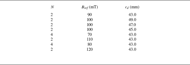


 Open access