





1 Introduction
Due to the prevalence of complex networked systems in nature and technology, a topic of growing interest has been the distributed cooperative control of agents that receive and transmit data through their neighbours [Reference Mesbahi and Egerstedt20]. In this context, the consensus problem is a fundamental problem that has been intensively studied in computer science and control theory [Reference Barborak, Malek and Dahbura2, Reference Olfati-Saber, Fax and Murray26]. The consensus problem entails a design of a distributed protocol that agents in the network can follow to reach an agreement over a certain quantity. The idea is to use only local information from the neighbourhood of each agent to achieve a global objective, and consensus protocols over various network topologies and dynamical environments have been reported in the literature [Reference Amirkhani and Barshooi1, Reference Boudin, Salvarani and Trélat5, Reference Jenabzadeh, Shu, Huang, Zhu, Shang and Gui14, Reference Li, Shang, Wang and Ma16, Reference Qin, Ma, Shi and Wang27].
Despite much work having been done on traditional consensus problems, where the states of agents can take any scalar or vector in the space, the consideration of state constraints is of importance to ensure wide applications in areas like motion planning, formation control and social dynamics, where agent states are often limited to given sets [Reference Nedić, Ozdaglar and Parrilo24]. Apparently, the requirement of the state constraints turns an otherwise potentially linear system into a nonlinear system, posing a challenge in the analysis of consensus behaviour. The interval consensus problem [Reference Fontan, Shi, Hu and Altafini8] (also known as consensus with soft constraints [Reference Shang34]) allows each agent to impose an upper bound and a lower bound independently to saturate the values it transmits to its neighbours. It is shown that if the intervals defined by the bounds of agents have a nonempty intersection, the system with a connected communication topology can converge to a common value within this intersection.
The interval consensus is radically different from other state-constrained consensus with hard-wired constraint sets. In these works, projection-based protocols and barrier functions are often used to ensure the trajectories of the agents remain in the convex constraint sets and the initial conditions of the system should be inside the same constrained sets; see for example, [Reference Borghi, Herty and Pareschi4, Reference Fu, Wen and Yu9, Reference Lin and Ren17, Reference Nedić, Ozdaglar and Parrilo24, Reference Shang30, Reference Shang37]. In contrast, the bounds proposed by the agents in the interval consensus framework only saturate the values agents transmit to their neighbours, so both the initial states and the transient trajectories may be outside the intervals. This framework is appropriate for distributed implementation and ideal in applications where each agent nominates an admissible region for the consensus to happen. For example, in social interactions, individuals are found to express their opinions within a comfort interval conforming to certain social norms or external observers [Reference Hoeben, Steenbeek and Pauwels13, Reference Monahan and Filler22, Reference Shang32]; in power management and load sharing among a group of units, each unit only accepts the workload within the range of its allocated capacity or resources [Reference Fan, Guo, Peng, Yang, Liu and Liu7, Reference Nahata, Turan and Ferrari-Trecate23]. A range of interval consensus protocols have been developed to address consensus under random networks [Reference Fu, Qin, Wu, Zheng and Kang10], state-dependent networks [Reference Shang35], signed networks [Reference Su, Wang and Gao40], higher-order dynamics [Reference Tian, Mei, Tian and Ma41] and Byzantine behaviour [Reference Shang31], as well as in applications concerning flocking dynamics [Reference Qin, Ma, Yi and Wang28], sampled data [Reference Zou, Zuo, Xia and Basin48] and social networks [Reference Shang33, Reference Shang34], to name a few.
In both traditional and interval consensus problems, agents exchange their states with neighbours explicitly with the aim of reaching an agreement. These consensus protocols pose a security risk of leaking sensitive information as the initial states of the system may be exposed to malicious agents in the network or external eavesdroppers tapping communication links [Reference Lu and Zhu19, Reference Shen, Huang, Liu, Xue, Zhuang, Sun and Ying39]. In most cooperative control and consensus coordination scenarios, including those mentioned above like social opinion dynamics and load-sharing systems, the agents desire to reach a consensus, but at the same time keep their initial conditions confidential. To this end, varied privacy-preserving consensus protocols have been proposed in the literature. A commonly used strategy is the differential privacy framework [Reference Nozari, Tallapragada and Cortés25, Reference Qin, He, Fang and Lam29, Reference Wang, Lam and Lin44], where random noises are introduced to obfuscate the state information. This strategy weakens the accuracy of the consensus protocols and the convergence under the differential privacy framework can only be guaranteed in probabilistic senses. Similar strategies in this flavour include methods involving correlated or variance-decaying noises [Reference He, Cai, Zhao, Cheng and Guan12, Reference Mo and Murray21]. Another class of designs relies on homomorphic encryption of the agents’ states (see for example, [Reference Chen, Liu and Liu6, Reference Hadjicostis and Domínguez-García11, Reference Lazzeretti, Horn, Braca and Willett15, Reference Yazhini, Samidurai and Shang46]). The cryptography-based methods often need an aggregative centralized third party, and suffer from hefty overhead in computation and communication. A machine learning based method has also been considered recently in [Reference Lu, Yu and Suri18] to guarantee privacy for consensus seeking, but the federated learning algorithm used therein is complex and resource-intensive. Moreover, these existing privacy-preserving consensus strategies do not apply to the more general interval consensus problem. The imposed interval constraints make the agents’ states more likely to be revealed as they constantly confine the transmitted values within the same finite range in each iterative update.
To cope with the challenge of guaranteeing privacy in the interval consensus problems, we propose a new design consisting of state decomposition, where each agent divides its state into two sub-states ( $\alpha $
-type state and
$\alpha $
-type state and $\beta $
-type state) and the
$\beta $
-type state) and the $\alpha $
-type state is revealed to its neighbours, but the
$\alpha $
-type state is revealed to its neighbours, but the $\beta $
-type state can only interact with its corresponding
$\beta $
-type state can only interact with its corresponding $\alpha $
-type state. The protocol is purely distributed and of low complexity. We show that the interval consensus can be achieved and the initial states of the agents are kept private if the underlying network topology is connected and the intersection of the intervals is nonempty. It is worth mentioning that our state decomposition mechanism leads to a coupled system with time-varying weights, thereby invalidating the convergence analysis previously applied in the interval consensus problems [Reference Fontan, Shi, Hu and Altafini8, Reference Fu, Qin, Wu, Zheng and Kang10, Reference Shang34, Reference Su, Wang and Gao40] (see Remark 3.3). However, we note that similar ideas of state decomposition or augmentation have been adopted in [Reference Shang38, Reference Wang43, Reference Wang, Lu, Zheng and Shi45, Reference Zhang, Li, Wang, Louati and Chen47] to solve privacy-preserving average consensus problems. However, these works require symmetric edge weights of the network and the transmitted values in the network have to be unsaturated. These restrictions are lifted in our design enabling the implementation of interval consensus with privacy preservation (see Remark 3.6).
$\alpha $
-type state. The protocol is purely distributed and of low complexity. We show that the interval consensus can be achieved and the initial states of the agents are kept private if the underlying network topology is connected and the intersection of the intervals is nonempty. It is worth mentioning that our state decomposition mechanism leads to a coupled system with time-varying weights, thereby invalidating the convergence analysis previously applied in the interval consensus problems [Reference Fontan, Shi, Hu and Altafini8, Reference Fu, Qin, Wu, Zheng and Kang10, Reference Shang34, Reference Su, Wang and Gao40] (see Remark 3.3). However, we note that similar ideas of state decomposition or augmentation have been adopted in [Reference Shang38, Reference Wang43, Reference Wang, Lu, Zheng and Shi45, Reference Zhang, Li, Wang, Louati and Chen47] to solve privacy-preserving average consensus problems. However, these works require symmetric edge weights of the network and the transmitted values in the network have to be unsaturated. These restrictions are lifted in our design enabling the implementation of interval consensus with privacy preservation (see Remark 3.6).
In applications such as power management and load sharing, each unit specifies a feasible interval representing the range of workload it can safely accommodate. Achieving a balanced operating point, therefore, amounts to an interval consensus problem in which all units must agree on a final value that lies inside the intersection of these capacity intervals. However, existing interval consensus protocols require agents to repeatedly exchange explicit state values, from which an adversary may infer sensitive operational information such as initial load levels or reserve margins. This makes direct deployment impractical in real power networks. The decomposition and weighting mechanisms proposed in this paper enable units to participate in the consensus process using only saturated and partially masked state components, preventing both neighbours and external eavesdroppers from reconstructing the actual initial loads. At the same time, the network is still guaranteed to reach a common value inside the feasible intersection. Thus, the proposed method provides a privacy-preserving way to coordinate load sharing while respecting individual capacity limits.
The structure of the paper is as follows. Section 2 formulates the interval consensus problem, and introduces the decomposition and weighting mechanisms that constitute the privacy-preserving protocol. Section 3 establishes the main theoretical results, showing that the proposed method guarantees both convergence of the interval consensus and preservation of the agents’ initial states against adversaries. Section 4 presents numerical simulations that illustrate the behaviour of the protocol, verify the theoretical findings and demonstrate the effect of the decomposition mechanism on convergence. Section 5 concludes the paper.
2 Problem formulation
2.1 Interval consensus
Consider a network system by a weighted directed graph $G=(V,E,A)$
, where the vertex set
$G=(V,E,A)$
, where the vertex set $V=\{v_1,v_2,\ldots ,v_n\}$
represents the group of n agents in the network,
$V=\{v_1,v_2,\ldots ,v_n\}$
represents the group of n agents in the network, $E\subseteq V\times V$
is the edge set and
$E\subseteq V\times V$
is the edge set and $A=A(t)$
is the weighted adjacency matrix potentially relying on time
$A=A(t)$
is the weighted adjacency matrix potentially relying on time $t\in \mathbb {N}$
. The graph G is a (time-dependent) bidirectional graph, meaning that it is essentially undirected, but it can have different weights for the two orientations of an edge. Specifically, for a given time step
$t\in \mathbb {N}$
. The graph G is a (time-dependent) bidirectional graph, meaning that it is essentially undirected, but it can have different weights for the two orientations of an edge. Specifically, for a given time step $t\in \mathbb {N}$
,
$t\in \mathbb {N}$
, $a_{ij}(t),a_{ji}(t)>0$
if
$a_{ij}(t),a_{ji}(t)>0$
if $(v_j,v_i)\in E$
and
$(v_j,v_i)\in E$
and $a_{ij}(t)=a_{ji}(t)=0$
otherwise. Here, to fix the notation,
$a_{ij}(t)=a_{ji}(t)=0$
otherwise. Here, to fix the notation, $(v_j,v_i)$
represents a directed edge from
$(v_j,v_i)$
represents a directed edge from $v_j$
to
$v_j$
to $v_i$
and it is associated with the weight
$v_i$
and it is associated with the weight $a_{ij}(t)$
. We assume
$a_{ij}(t)$
. We assume $0<a_{ij}(t)\le 1$
if
$0<a_{ij}(t)\le 1$
if $a_{ij}(t)\not =0$
. The neighbourhood of
$a_{ij}(t)\not =0$
. The neighbourhood of $v_i\in V$
is denoted by
$v_i\in V$
is denoted by ${N_i=\{v_j\in V: (v_i,v_j)\in E\}}$
. As both directions of an edge appear simultaneously, we do not differentiate between in-neighbourhood and out-neighbourhood. Let
${N_i=\{v_j\in V: (v_i,v_j)\in E\}}$
. As both directions of an edge appear simultaneously, we do not differentiate between in-neighbourhood and out-neighbourhood. Let $\Delta =\max _{v_i\in V}|N_i|$
be the maximum degree of the graph G. Note that
$\Delta =\max _{v_i\in V}|N_i|$
be the maximum degree of the graph G. Note that $\Delta $
and
$\Delta $
and $N_i$
are not functions of t.
$N_i$
are not functions of t.
For each agent $v_i\in V$
, we define an interval
$v_i\in V$
, we define an interval $\Theta _i=[\underline {\theta }_i,\overline {\theta }_i]$
and an increasing function
$\Theta _i=[\underline {\theta }_i,\overline {\theta }_i]$
and an increasing function $g_i:\mathbb {R}\rightarrow \Theta _i$
satisfying
$g_i:\mathbb {R}\rightarrow \Theta _i$
satisfying
 $$ \begin{align} g_i(z) = \begin{cases}{ll} \underline{\theta}_i,& z<\underline{\theta}_i;\\ z,&\underline{\theta}_i\le z\le\overline{\theta}_i;\\ \overline{\theta}_i,& z>\overline{\theta}_i. \end{cases} \end{align} $$
The agent $v_i$
updates its state following the protocol
$v_i$
updates its state following the protocol
 $$ \begin{align} x_i(t+1)=x_i(t)+\varepsilon\sum_{v_j\in N_i}a_{ij}(t)(g_j(x_j(t))-x_i(t)),\quad t\in\mathbb{N}, \end{align} $$
where $x_i(t)\in \mathbb {R}$
means the state of agent
$x_i(t)\in \mathbb {R}$
means the state of agent $v_i$
and
$v_i$
and $0<\varepsilon <\Delta ^{-1}$
is the control gain. The information transmitted from a neighbour
$0<\varepsilon <\Delta ^{-1}$
is the control gain. The information transmitted from a neighbour $v_j$
is saturated by the function
$v_j$
is saturated by the function $g_j$
. We assume that the interval
$g_j$
. We assume that the interval $\Theta _j$
is only known to the agent
$\Theta _j$
is only known to the agent $v_j$
itself. In other words, an agent
$v_j$
itself. In other words, an agent $v_i$
will receive the saturated value
$v_i$
will receive the saturated value $g_j(x_j(t))$
from its neighbour
$g_j(x_j(t))$
from its neighbour $v_j$
, but has no knowledge of
$v_j$
, but has no knowledge of $x_j(t)$
.
$x_j(t)$
.
Suppose that the intersection set $\bigcap _{i=1}^n\Theta _i\not =\emptyset $
. The objective of the interval consensus is to show that there exists a constant
$\bigcap _{i=1}^n\Theta _i\not =\emptyset $
. The objective of the interval consensus is to show that there exists a constant $\tilde {z}\in \bigcap _{i=1}^n\Theta _i$
such that
$\tilde {z}\in \bigcap _{i=1}^n\Theta _i$
such that $\lim _{t\rightarrow \infty }x_i(t)=\tilde {z}$
for any
$\lim _{t\rightarrow \infty }x_i(t)=\tilde {z}$
for any $v_i\in V$
and
$v_i\in V$
and $x_i(0)\in \mathbb {R}$
. In the next subsection, we design a decomposition approach and a weighting approach to facilitate the interval consensus while maintaining the privacy of initial states of the agents.
$x_i(0)\in \mathbb {R}$
. In the next subsection, we design a decomposition approach and a weighting approach to facilitate the interval consensus while maintaining the privacy of initial states of the agents.
Remark 2.1. The above framework (2.2) differs from the existing works regarding interval consensus (see for example, [Reference Fontan, Shi, Hu and Altafini8, Reference Fu, Qin, Wu, Zheng and Kang10, Reference Qin, Ma, Yi and Wang28, Reference Shang33, Reference Shang34, Reference Su, Wang and Gao40, Reference Zou, Zuo, Xia and Basin48]), where the underlying communication weights are usually assumed to be time-invariant, namely, $a_{ij}(t)\equiv a_{ij}$
for all
$a_{ij}(t)\equiv a_{ij}$
for all $v_i,v_j\in V$
and
$v_i,v_j\in V$
and $t\ge 0$
. In [Reference Shang31, Reference Shang35], the weights are allowed to depend on time, but they must follow some specific processes. In contrast, our weights in (2.2) can be chosen freely in general (see the weighting approach that appears later).
$t\ge 0$
. In [Reference Shang31, Reference Shang35], the weights are allowed to depend on time, but they must follow some specific processes. In contrast, our weights in (2.2) can be chosen freely in general (see the weighting approach that appears later).
2.2 Privacy-preserving mechanism
We consider two sorts of adversaries in this paper. The first is honest-but-curious agents. They are agents in the network G following the same protocol as others, but they attempt to learn the information of other agents. They may collude with other honest-but-curious agents to infer the information. The second adversary is eavesdroppers. They are external attackers, who have the knowledge of the network topology of G, and can monitor and learn transmitted messages along any edge in E. An eavesdropper appears to be more troublesome because it has more access to the network data, while an honest-but-curious agent, say $v_i$
, only knows information sent directly to it via (2.2). However, it is worth noting that the agent
$v_i$
, only knows information sent directly to it via (2.2). However, it is worth noting that the agent $v_i$
knows its own state
$v_i$
knows its own state $x_i(t)$
, which is not accessible to an eavesdropper. To ensure the privacy of initial conditions
$x_i(t)$
, which is not accessible to an eavesdropper. To ensure the privacy of initial conditions $\{x_i(0)\}_{v_i\in V}$
of the network against these two kinds of adversaries, we propose the following strategy.
$\{x_i(0)\}_{v_i\in V}$
of the network against these two kinds of adversaries, we propose the following strategy.
2.2.1 Decomposition approach.
Each vertex $v_i$
decomposes its state
$v_i$
decomposes its state $x_i$
into the
$x_i$
into the $\alpha $
-type state
$\alpha $
-type state $x_i^{\alpha }$
and the
$x_i^{\alpha }$
and the $\beta $
-type state
$\beta $
-type state $x_i^{\beta }$
; see Figure 1 for an illustration. The initial values
$x_i^{\beta }$
; see Figure 1 for an illustration. The initial values $x_i^{\alpha }(0)\in \mathbb {R}$
and
$x_i^{\alpha }(0)\in \mathbb {R}$
and $x_i^{\beta }(0)\in \mathbb {R}$
are chosen arbitrarily at random. The sub-state
$x_i^{\beta }(0)\in \mathbb {R}$
are chosen arbitrarily at random. The sub-state $x_i^{\alpha }$
inherits the behaviour of
$x_i^{\alpha }$
inherits the behaviour of $x_i$
and interacts with the neighbours of
$x_i$
and interacts with the neighbours of $v_i$
over G. The sub-state
$v_i$
over G. The sub-state $x_i^{\beta }$
only communicates with
$x_i^{\beta }$
only communicates with $x_i^{\alpha }$
with the edge weights characterized by
$x_i^{\alpha }$
with the edge weights characterized by $a_{i,\alpha \beta }(t)$
and
$a_{i,\alpha \beta }(t)$
and $a_{i,\beta \alpha }(t)$
. Here,
$a_{i,\beta \alpha }(t)$
. Here, $a_{i,\alpha \beta }(t)$
is associated with the edge from the
$a_{i,\alpha \beta }(t)$
is associated with the edge from the $\beta $
-type state to the
$\beta $
-type state to the $\alpha $
-type state and
$\alpha $
-type state and $a_{i,\beta \alpha }(t)$
is associated with the edge from the
$a_{i,\beta \alpha }(t)$
is associated with the edge from the $\alpha $
-type state to the
$\alpha $
-type state to the $\beta $
-type state.
$\beta $
-type state.
A schematic illustration of state decomposition for a vertex $v_i$
with degree 2 in G.
$v_i$
with degree 2 in G.

In view of (2.2), the system dynamics under the decomposition approach can be rewritten as follows:
 $$ \begin{align} \begin{cases} x_i^{\alpha}(t+1)=x_i^{\alpha}(t)+\varepsilon\sum_{v_j\in N_i}a_{ij}(t)(g_j(x_j^{\alpha}(t))-x_i^{\alpha}(t))\\ \qquad \ \qquad +\ \varepsilon a_{i,\alpha\beta}(t)(g_i(x_i^{\beta}(t))-x_i^{\alpha}(t)),\\ x_i^{\beta}(t+1)=x_i^{\beta}(t)+\varepsilon a_{i,\beta\alpha}(t)(g_i(x_i^{\alpha}(t))-x_i^{\beta}(t)), \end{cases} \end{align} $$
where $t\in \mathbb {N}$
,
$t\in \mathbb {N}$
, $v_i\in V$
and
$v_i\in V$
and $0<\varepsilon <(\Delta +1)^{-1}$
. Clearly, the state decomposition can be viewed as a decomposition of vertices. For this reason, we also refer to
$0<\varepsilon <(\Delta +1)^{-1}$
. Clearly, the state decomposition can be viewed as a decomposition of vertices. For this reason, we also refer to $\alpha $
-type vertices and
$\alpha $
-type vertices and $\beta $
-type vertices accordingly.
$\beta $
-type vertices accordingly.
2.2.2 Weighting approach.
For $v_i, v_j\in V$
, the initial edge weights
$v_i, v_j\in V$
, the initial edge weights $a_{ij}(0)\in \mathbb {R}$
,
$a_{ij}(0)\in \mathbb {R}$
, $a_{ji}(0)\in \mathbb {R}$
,
$a_{ji}(0)\in \mathbb {R}$
, $a_{i,\alpha \beta }(0)\in \mathbb {R}$
and
$a_{i,\alpha \beta }(0)\in \mathbb {R}$
and $a_{i,\beta \alpha }(0)\in \mathbb {R}$
are chosen arbitrarily at random (if
$a_{i,\beta \alpha }(0)\in \mathbb {R}$
are chosen arbitrarily at random (if $(v_i,v_j)\in E$
). When
$(v_i,v_j)\in E$
). When $t\ge 1$
, there exists a constant
$t\ge 1$
, there exists a constant $\xi>0$
such that
$\xi>0$
such that $\xi <a_{ij}(t),a_{ji}(t)\le 1$
if
$\xi <a_{ij}(t),a_{ji}(t)\le 1$
if $(v_i,v_j)\in E$
. Moreover,
$(v_i,v_j)\in E$
. Moreover, $\xi <a_{i,\alpha \beta }(t),a_{i,\beta \alpha }(t)\le 1$
for
$\xi <a_{i,\alpha \beta }(t),a_{i,\beta \alpha }(t)\le 1$
for $t\ge 1$
.
$t\ge 1$
.
For $v_i\in V$
and
$v_i\in V$
and $t\in \mathbb {N}$
, define a set
$t\in \mathbb {N}$
, define a set $\Gamma _i(t)$
to be the information accessible to
$\Gamma _i(t)$
to be the information accessible to $v_i$
at time t. Let
$v_i$
at time t. Let $\Gamma _i=\bigcup _{t\in \mathbb {N}}\Gamma _i(t)$
be the aggregated information available to
$\Gamma _i=\bigcup _{t\in \mathbb {N}}\Gamma _i(t)$
be the aggregated information available to $v_i$
. Suppose
$v_i$
. Suppose $v_i$
is an adversary looking to infer the initial state of another agent
$v_i$
is an adversary looking to infer the initial state of another agent $v_j\in V$
. We say the privacy of the initial condition
$v_j\in V$
. We say the privacy of the initial condition $x_j(0)$
is preserved against
$x_j(0)$
is preserved against $v_i$
if for any
$v_i$
if for any $\hat {x}_j(0)\not =x_j(0)$
, there exists an associated
$\hat {x}_j(0)\not =x_j(0)$
, there exists an associated $\hat {\Gamma }_i$
such that
$\hat {\Gamma }_i$
such that $\hat {\Gamma }_i=\Gamma _i$
under a privacy-preserving mechanism. The idea is intuitively clear as follows. If any change of
$\hat {\Gamma }_i=\Gamma _i$
under a privacy-preserving mechanism. The idea is intuitively clear as follows. If any change of $x_j(0)$
cannot be distinguished by the adversary
$x_j(0)$
cannot be distinguished by the adversary $v_i$
through the implementation of the privacy-preserving mechanism,
$v_i$
through the implementation of the privacy-preserving mechanism, $v_i$
has no way to infer the initial condition
$v_i$
has no way to infer the initial condition $x_j(0)$
with any guaranteed accuracy. We show that the above decomposition approach and weighting approach form such a privacy-preserving mechanism (see Theorem 3.5).
$x_j(0)$
with any guaranteed accuracy. We show that the above decomposition approach and weighting approach form such a privacy-preserving mechanism (see Theorem 3.5).
3 Main results
3.1 Consensus analysis
In this subsection, we show the convergence of the networked system under the proposed privacy-preserving mechanism when the intersection of the imposed intervals is not empty. Let $\theta ^*=\min _{v_i\in V}\overline {\theta }_i$
and
$\theta ^*=\min _{v_i\in V}\overline {\theta }_i$
and $\theta _*=\max _{v_i\in V}\underline {\theta }_i$
. Apparently, the condition
$\theta _*=\max _{v_i\in V}\underline {\theta }_i$
. Apparently, the condition $\bigcap _{i=1}^n\Theta _i\not =\emptyset $
is equivalent to
$\bigcap _{i=1}^n\Theta _i\not =\emptyset $
is equivalent to $\bigcap _{i=1}^n\Theta _i=[\theta _*,\theta ^*]$
with
$\bigcap _{i=1}^n\Theta _i=[\theta _*,\theta ^*]$
with $\theta _*\le \theta ^*$
. Moreover, it is easy to see that the system (2.3) can be reorganized in the following format, which we heavily use in the proof of Theorem 3.1:
$\theta _*\le \theta ^*$
. Moreover, it is easy to see that the system (2.3) can be reorganized in the following format, which we heavily use in the proof of Theorem 3.1:
 $$ \begin{align} \begin{cases} x_i^{\alpha}(t+1)=(1-\varepsilon\sum_{v_j\in N_i}a_{ij}(t)-\varepsilon a_{i,\alpha\beta}(t))x_i^{\alpha}(t)\\ \qquad \qquad \ +\ \varepsilon\sum_{v_j\in N_i}a_{ij}(t)g_j(x_j^{\alpha}(t))+ \varepsilon a_{i,\alpha\beta}(t)g_i(x_i^{\beta}(t)),\\ x_i^{\beta}(t+1)=(1-\varepsilon a_{i,\beta\alpha}(t))x_i^{\beta}(t)+\varepsilon a_{i,\beta\alpha}(t)g_i(x_i^{\alpha}(t)).\end{cases} \end{align} $$
Theorem 3.1. Suppose that the intersection set $[\theta _*,\theta ^*]$
is not empty and the graph G is connected. If
$[\theta _*,\theta ^*]$
is not empty and the graph G is connected. If $0<\varepsilon <(\Delta +1)^{-1}$
, then under the decomposition approach and the weighting approach, the following holds. For any initial condition
$0<\varepsilon <(\Delta +1)^{-1}$
, then under the decomposition approach and the weighting approach, the following holds. For any initial condition $\{x_i(0)\}_{v_i\in V}$
, there exists
$\{x_i(0)\}_{v_i\in V}$
, there exists $\tilde {z}\in [\theta _*,\theta ^*]$
such that
$\tilde {z}\in [\theta _*,\theta ^*]$
such that $\lim _{t\rightarrow \infty }x_i(t)=\tilde {z}$
for
$\lim _{t\rightarrow \infty }x_i(t)=\tilde {z}$
for $v_i\in V$
.
$v_i\in V$
.
Remark 3.2. Theorem 3.1 shows that our proposed privacy-preserving mechanism enables interval consensus. The assumptions in this theorem are essentially necessary. Clearly, the nonemptiness of the intersection is necessary. If G is not connected, consensus cannot be reached over the whole network topology because an agent in one component will not receive any information from another component. The condition $0<\varepsilon <(\Delta +1)^{-1}$
for the step size is also well known to be a necessary condition for the convergence of discrete-time Laplacian-like systems; (see for example, [Reference Olfati-Saber, Fax and Murray26, Remark 3]).
$0<\varepsilon <(\Delta +1)^{-1}$
for the step size is also well known to be a necessary condition for the convergence of discrete-time Laplacian-like systems; (see for example, [Reference Olfati-Saber, Fax and Murray26, Remark 3]).
Proof. The interval consensus is proved in several steps. We define two functions $\overline {\varphi }(t)=\max \{\max _{v_i\in V}x_i^{\alpha }(t),\max _{v_i\in V}x_i^{\beta }(t),\theta ^*\}$
and
$\overline {\varphi }(t)=\max \{\max _{v_i\in V}x_i^{\alpha }(t),\max _{v_i\in V}x_i^{\beta }(t),\theta ^*\}$
and $\underline {\varphi }(t)=\min \{\min _{v_i\in V}x_i^{\alpha }(t), \min _{v_i\in V}x_i^{\beta }(t),\, \theta _*\}$
. Clearly,
$\underline {\varphi }(t)=\min \{\min _{v_i\in V}x_i^{\alpha }(t), \min _{v_i\in V}x_i^{\beta }(t),\, \theta _*\}$
. Clearly, $\overline {\varphi }(t)\ge \theta ^*\ge \theta _*\ge \underline {\varphi }(t)$
for
$\overline {\varphi }(t)\ge \theta ^*\ge \theta _*\ge \underline {\varphi }(t)$
for $t\in \mathbb {N}$
.
$t\in \mathbb {N}$
.
Step (i). We first show that the functions $\overline {\varphi }(t)$
and
$\overline {\varphi }(t)$
and $\underline {\varphi }(t)$
are monotonic when
$\underline {\varphi }(t)$
are monotonic when $t\ge 1$
. For
$t\ge 1$
. For $a\in \mathbb {R}$
, we define an increasing function
$a\in \mathbb {R}$
, we define an increasing function $\overline {f}_a(z)=\max \{z,a\}$
. Hence, by using (3.1), we have for
$\overline {f}_a(z)=\max \{z,a\}$
. Hence, by using (3.1), we have for $t\ge 1$
,
$t\ge 1$
,
 $$ \begin{align} \overline{\varphi}(t+1) & =\overline{f}_{\theta^*}\bigg(\max_{v_i\in V}\{x_i^{\alpha}(t+1),x_i^{\beta}(t+1)\}\bigg)\nonumber\\ &= \overline{f}_{\theta^*}\bigg(\max_{v_i\in V}\bigg\{\bigg(1-\varepsilon\sum_{v_j\in N_i}a_{ij}(t)-\varepsilon a_{i,\alpha\beta}(t)\bigg)x_i^{\alpha}(t)+\varepsilon\sum_{v_j\in N_i}a_{ij}(t)g_j(x_j^{\alpha}(t))\nonumber\\ &\quad + \varepsilon a_{i,\alpha\beta}(t)g_i(x_i^{\beta}(t)),(1-\varepsilon a_{i,\beta\alpha}(t))x_i^{\beta}(t)+\varepsilon a_{i,\beta\alpha}(t)g_i(x_i^{\alpha}(t))\bigg\}\bigg)\nonumber\\ & \le\overline{f}_{\theta^*}\bigg(\max_{v_i\in V}\bigg\{ \bigg(1-\varepsilon\sum_{v_j\in N_i}a_{ij}(t)-\varepsilon a_{i,\alpha\beta}(t)\bigg)\,\overline{f}_{\theta^*}(x_i^{\alpha}(t))+\varepsilon\sum_{v_j\in N_i}a_{ij}(t)\overline{f}_{\theta^*}(x_j^{\alpha}(t))\nonumber\\ &\quad + \varepsilon a_{i,\alpha\beta}(t)\overline{f}_{\theta^*}(x_i^{\beta}(t)),(1-\varepsilon a_{i,\beta\alpha}(t))\overline{f}_{\theta^*}(x_i^{\beta}(t))+\varepsilon a_{i,\beta\alpha}(t)\overline{f}_{\theta^*}(x_i^{\alpha}(t))\bigg\}\bigg), \end{align} $$
where we have used (2.1), the assumption $\varepsilon \in (0,(\Delta +1)^{-1})$
and the weighting mechanism. In view of the monotonicity of
$\varepsilon \in (0,(\Delta +1)^{-1})$
and the weighting mechanism. In view of the monotonicity of $\overline {f}_{\theta ^*}$
and the state decomposition, the right-hand side of (3.2) is not greater than
$\overline {f}_{\theta ^*}$
and the state decomposition, the right-hand side of (3.2) is not greater than
 $$ \begin{align} &\overline{f}_{\theta^*}\bigg(\max_{v_i\in V}\bigg\{ \bigg(1-\varepsilon\sum_{v_j\in N_i}a_{ij}(t)-\varepsilon a_{i,\alpha\beta}(t)\bigg)\,\overline{f}_{\theta^*}\bigg(\max_{v_i\in V}\{x_i^{\alpha}(t),x_i^{\beta}(t)\}\bigg)\nonumber\\&\qquad\ \ \ \,\qquad +\varepsilon\sum_{v_j\in N_i}a_{ij}(t)\overline{f}_{\theta^*}\bigg(\max_{v_i\in V}\{x_i^{\alpha}(t),x_i^{\beta}(t)\}\bigg)+\varepsilon a_{i,\alpha\beta}(t)\overline{f}_{\theta^*}\bigg(\max_{v_i\in V}\{x_i^{\alpha}(t),x_i^{\beta}(t)\}\bigg),\nonumber\\& \qquad\qquad (1-\varepsilon a_{i,\beta\alpha}(t))\overline{f}_{\theta^*}\bigg(\max_{v_i\in V}\{x_i^{\alpha}(t),x_i^{\beta}(t)\}\bigg)+\varepsilon a_{i,\beta\alpha}(t)\overline{f}_{\theta^*}\bigg(\max_{v_i\in V}\{x_i^{\alpha}(t),x_i^{\beta}(t)\}\bigg)\bigg\}\bigg)\nonumber\\& \quad = \overline{f}_{\theta^*}\bigg(\overline{f}_{\theta^*}\bigg(\max_{v_i\in V}\{ x_i^{\alpha}(t),x_i^{\beta}(t)\}\bigg)\bigg)\nonumber\\& \quad =\overline{\varphi}(t). \end{align} $$
This means $\overline {\varphi }(t)$
is decreasing for
$\overline {\varphi }(t)$
is decreasing for $t\ge 1$
. Likewise, we can define an increasing function
$t\ge 1$
. Likewise, we can define an increasing function $\underline {f}_a(z)=\min \{z,a\}$
for
$\underline {f}_a(z)=\min \{z,a\}$
for $a\in \mathbb {R}$
. Noting
$a\in \mathbb {R}$
. Noting $\underline {f}_{\theta _*}(\min _{v_i\in V}\{ x_i^{\alpha }(t),x_i^{\beta }(t)\})=\underline {\varphi }(t)$
, and arguing as (3.2) and (3.3), we can derive
$\underline {f}_{\theta _*}(\min _{v_i\in V}\{ x_i^{\alpha }(t),x_i^{\beta }(t)\})=\underline {\varphi }(t)$
, and arguing as (3.2) and (3.3), we can derive $\underline {\varphi }(t+1)\ge \underline {\varphi }(t)$
for
$\underline {\varphi }(t+1)\ge \underline {\varphi }(t)$
for $t\ge 1$
.
$t\ge 1$
.
Step (ii). From Step (i), we know that $\overline {\varphi }(t)$
and
$\overline {\varphi }(t)$
and $\underline {\varphi }(t)$
are monotonic and bounded. Therefore, there exist
$\underline {\varphi }(t)$
are monotonic and bounded. Therefore, there exist $\varphi ^*,\varphi _*\in \mathbb {R}$
such that
$\varphi ^*,\varphi _*\in \mathbb {R}$
such that $\lim _{t\rightarrow \infty }\overline {\varphi }(t)=\varphi ^*$
and
$\lim _{t\rightarrow \infty }\overline {\varphi }(t)=\varphi ^*$
and $\lim _{t\rightarrow \infty }\underline {\varphi }(t)=\varphi _*$
. Therefore,
$\lim _{t\rightarrow \infty }\underline {\varphi }(t)=\varphi _*$
. Therefore, $\varphi ^*\ge \theta ^*\ge \theta _*\ge \varphi _*$
. Here, we aim to prove
$\varphi ^*\ge \theta ^*\ge \theta _*\ge \varphi _*$
. Here, we aim to prove $\theta _*=\varphi _*$
. The proof of
$\theta _*=\varphi _*$
. The proof of $\varphi ^*=\theta ^*$
is analogous and hence omitted.
$\varphi ^*=\theta ^*$
is analogous and hence omitted.
Suppose in contrast $\theta _*>\varphi _*$
. For any time step
$\theta _*>\varphi _*$
. For any time step $s>0$
, there exists an agent
$s>0$
, there exists an agent $v_{i_0}$
such that either (a)
$v_{i_0}$
such that either (a) $x^{\alpha }_{i_0}(s)=\min _{v_j\in V}\{x_j^{\alpha }(s),x_j^{\beta }(s)\}\le \varphi _*<\theta _*$
or (b)
$x^{\alpha }_{i_0}(s)=\min _{v_j\in V}\{x_j^{\alpha }(s),x_j^{\beta }(s)\}\le \varphi _*<\theta _*$
or (b) $x^{\beta }_{i_0}(s)=\min _{v_j\in V}\{x_j^{\alpha }(s),x_j^{\beta }(s)\}\le \varphi _*<\theta _*$
. To avoid examining both scenarios (a) and (b), in the rest of the proof of Theorem 3.1, we introduce the following notation to ease the presentation. Let
$x^{\beta }_{i_0}(s)=\min _{v_j\in V}\{x_j^{\alpha }(s),x_j^{\beta }(s)\}\le \varphi _*<\theta _*$
. To avoid examining both scenarios (a) and (b), in the rest of the proof of Theorem 3.1, we introduce the following notation to ease the presentation. Let $\tilde {V}=\{v_1,v_2,\ldots , v_n,v_{n+1},v_{n+2},\ldots , v_{2n}\}$
, where
$\tilde {V}=\{v_1,v_2,\ldots , v_n,v_{n+1},v_{n+2},\ldots , v_{2n}\}$
, where $v_i$
and
$v_i$
and $v_{n+i}$
are the
$v_{n+i}$
are the $\alpha $
-type and
$\alpha $
-type and $\beta $
-type vertices, respectively, for the same original vertex
$\beta $
-type vertices, respectively, for the same original vertex $v_i$
in
$v_i$
in $G\, (1\le i\le n)$
. The corresponding graph over
$G\, (1\le i\le n)$
. The corresponding graph over $\tilde {V}$
is denoted by
$\tilde {V}$
is denoted by $\tilde {G}$
. The neighbourhood of a vertex
$\tilde {G}$
. The neighbourhood of a vertex $v_j\in \tilde {V}$
in
$v_j\in \tilde {V}$
in $\tilde {G}$
is denoted by
$\tilde {G}$
is denoted by $\tilde {N}_j$
. Likewise, we rewrite the states of vertices by
$\tilde {N}_j$
. Likewise, we rewrite the states of vertices by $y_i=x^{\alpha }_i$
and
$y_i=x^{\alpha }_i$
and $y_{n+i}=x^{\beta }_i\, (1\le i\le n)$
. Denote by
$y_{n+i}=x^{\beta }_i\, (1\le i\le n)$
. Denote by $a_{i,\alpha \beta }=a_{i, n+i}$
and
$a_{i,\alpha \beta }=a_{i, n+i}$
and $a_{i,\beta \alpha }=a_{n+i,i}\, (1\le i\le n)$
. It is easy to see that with the above notation, the system (2.3) or (3.1) reduces to the original format of (2.2) (with
$a_{i,\beta \alpha }=a_{n+i,i}\, (1\le i\le n)$
. It is easy to see that with the above notation, the system (2.3) or (3.1) reduces to the original format of (2.2) (with $x_i$
replaced by
$x_i$
replaced by $y_i$
). In the rest of the proof of Theorem 3.1, we stick to this framework, which largely simplifies our presentation.
$y_i$
). In the rest of the proof of Theorem 3.1, we stick to this framework, which largely simplifies our presentation.
According to the above comment, for any time step $s>0$
, there exists an agent
$s>0$
, there exists an agent $v_{i_0}\in \tilde {V}$
such that
$v_{i_0}\in \tilde {V}$
such that $y_{i_0}(s)=\min _{v_j\in \tilde {V}}\{y_j(s)\}\le \varphi _*<\theta _*$
. Since G is connected,
$y_{i_0}(s)=\min _{v_j\in \tilde {V}}\{y_j(s)\}\le \varphi _*<\theta _*$
. Since G is connected, $\tilde {G}$
is also connected. We take
$\tilde {G}$
is also connected. We take $v_{i_1}$
as a neighbour of
$v_{i_1}$
as a neighbour of $v_{i_0}$
and we have
$v_{i_0}$
and we have
 $$ \begin{align} y_{i_1}(s+1)& = \bigg(1-\varepsilon\sum_{v_j\in \tilde{N}_{i_1}}a_{i_1j}(s)\bigg)y_{i_1}(s)+\varepsilon\sum_{v_j\in \tilde{N}_{i_1}}a_{i_1j}(s)g_j(y_j(s))\nonumber\\[5pt] & =\bigg(1-\varepsilon\sum_{v_j\in \tilde{N}_{i_1}}a_{i_1j}(s)\bigg)y_{i_1}(s)+\varepsilon\sum_{v_j\in \tilde{N}_{i_1},v_j\not=v_{i_0}}a_{i_1j}(s)g_j(y_j(s))+\varepsilon a_{i_1i_0}(s)g_{i_0}(y_{i_0}(s))\nonumber\\[5pt] & \le\bigg(1-\varepsilon\sum_{v_j\in \tilde{N}_{i_1}}a_{i_1j}(s)\bigg)\,\overline{f}_{\theta^*}\bigg(\max_{v_j\in\tilde{V}}y_j(s)\bigg)\nonumber\\[5pt] &\quad +\varepsilon\sum_{v_j\in \tilde{N}_{i_1},v_j\not=v_{i_0}}a_{i_1j}(s)\overline{f}_{\theta^*}\bigg(\max_{v_j\in\tilde{V}}y_j(s)\bigg) +\varepsilon a_{i_1i_0}(s)\theta_*\nonumber\\[5pt] &=(1-\varepsilon a_{i_1i_0}(s))\overline{f}_{\theta^*}\bigg(\max_{v_j\in\tilde{V}}y_j(s)\bigg)+\varepsilon a_{i_1i_0}(s)\theta_*, \end{align} $$
where we have noted that $g_{i_0}(y_{i_0}(s))\le g_{i_0}(\varphi _*)\le \theta _*$
since
$g_{i_0}(y_{i_0}(s))\le g_{i_0}(\varphi _*)\le \theta _*$
since $g_{i_0}$
is an increasing function and
$g_{i_0}$
is an increasing function and $\underline {\theta }_{i_0}\le \theta _*$
. Define a constant c as follows:
$\underline {\theta }_{i_0}\le \theta _*$
. Define a constant c as follows:
 $$ \begin{align} 0<c=\min\{\varepsilon\xi,1-\varepsilon(\Delta+1)\}<1. \end{align} $$
Note that $c\le \varepsilon a_{i_1i_0}(s)$
and
$c\le \varepsilon a_{i_1i_0}(s)$
and $\overline {f}_{\theta ^*}(\max _{v_j\in \tilde {V}}y_j(s))\ge \theta _*$
by the weighting approach. Therefore, the right-hand side of (3.4) is not greater than
$\overline {f}_{\theta ^*}(\max _{v_j\in \tilde {V}}y_j(s))\ge \theta _*$
by the weighting approach. Therefore, the right-hand side of (3.4) is not greater than
 $$ \begin{align} (1-c)\overline{f}_{\theta^*}\bigg(\max_{v_j\in\tilde{V}}y_j(s)\bigg)+c\theta_*. \end{align} $$
Similarly, we obtain
 $$ \begin{align} y_{i_0}(s+1) & =\bigg(1-\varepsilon\sum_{v_j\in \tilde{N}_{i_0}}a_{i_0j}(s)\bigg)y_{i_0}(s)+\varepsilon\sum_{v_j\in \tilde{N}_{i_0}}a_{i_0j}(s)g_j(y_j(s))\nonumber\\ & \le\bigg(1-\varepsilon\sum_{v_j\in \tilde{N}_{i_0}}a_{i_0j}(s)\bigg)\theta_*+\varepsilon\sum_{v_j\in \tilde{N}_{i_0}}a_{i_0j}(s)\overline{f}_{\theta^*}\bigg(\max_{v_j\in\tilde{V}}y_j(s)\bigg)\nonumber\\ &\le c\theta_*+(1-c)\overline{f}_{\theta^*}\bigg(\max_{v_j\in\tilde{V}}y_j(s)\bigg), \end{align} $$
where we have applied $\theta _*\le \overline {f}_{\theta ^*}(\max _{v_j\in \tilde {V}}y_j(s))$
,
$\theta _*\le \overline {f}_{\theta ^*}(\max _{v_j\in \tilde {V}}y_j(s))$
, $c\le 1-\varepsilon \sum _{v_j\in \tilde {N}_{i_0}}a_{i_0j}(s)$
and (3.5). Combining (3.4), (3.6) and (3.7), we conclude that for
$c\le 1-\varepsilon \sum _{v_j\in \tilde {N}_{i_0}}a_{i_0j}(s)$
and (3.5). Combining (3.4), (3.6) and (3.7), we conclude that for $k=i_0,i_1$
,
$k=i_0,i_1$
,
 $$ \begin{align} y_k(s+1)\le c\theta_*+(1-c)\overline{f}_{\theta^*}\bigg(\max_{v_j\in\tilde{V}}y_j(s)\bigg). \end{align} $$
At time step $s+2$
, we obtain for
$s+2$
, we obtain for $k=i_0,i_1$
,
$k=i_0,i_1$
,
 $$ \begin{align} x_k(s+2) & = \bigg(1-\varepsilon\sum_{v_j\in \tilde{N}_k}a_{kj}(s+1)\bigg)y_k(s+1)+\varepsilon\sum_{v_j\in \tilde{N}_k}a_{kj}(s+1)g_j(y_j(s+1))\nonumber\\ & \le \bigg(1-\varepsilon\sum_{v_j\in \tilde{N}_k}a_{kj}(s+1)\bigg)\bigg(c\theta_*+(1-c)\overline{f}_{\theta^*}\bigg(\max_{v_j\in\tilde{V}}y_j(s)\bigg)\bigg)\nonumber\\ &\quad +\varepsilon\bigg(\sum_{v_j\in \tilde{N}_k}a_{kj}(s+1)\bigg)\,\overline{f}_{\theta^*}\bigg(\max_{v_j\in\tilde{V}}y_j(s)\bigg)\nonumber\\ & =c\theta_*+c\varepsilon\bigg(\sum_{v_j\in \tilde{N}_k}a_{kj}(s+1)\bigg)\bigg(\overline{f}_{\theta^*}\bigg(\max_{v_j\in\tilde{V}}y_j(s)\bigg)-\theta_*\bigg) +(1-c)\overline{f}_{\theta^*}\bigg(\max_{v_j\in\tilde{V}}y_j(s)\bigg) \end{align} $$
by using (3.8) and
 $$ \begin{align*} g_j(y_j(s+1))\le \overline{f}_{\theta^*}(y_j(s+1))\le\overline{f}_{\theta^*}\bigg(\max_{v_j\in\tilde{V}}y_j(s+1)\bigg) \le \overline{f}_{\theta^*}\bigg(\max_{v_j\in\tilde{V}}y_j(s)\bigg). \end{align*} $$
Since $\varepsilon \sum _{v_j\in \tilde {N}_k}a_{kj}(s+1)\le 1-c$
and
$\varepsilon \sum _{v_j\in \tilde {N}_k}a_{kj}(s+1)\le 1-c$
and $\overline {f}_{\theta ^*}(\max _{v_j\in \tilde {V}}y_j(s))-\theta _*\ge 0$
, the right-hand side of (3.9) is not greater than
$\overline {f}_{\theta ^*}(\max _{v_j\in \tilde {V}}y_j(s))-\theta _*\ge 0$
, the right-hand side of (3.9) is not greater than
 $$ \begin{align} &c\theta_*+c(1-c)\bigg(\overline{f}_{\theta^*}\bigg(\max_{v_j\in\tilde{V}}y_j(s)\bigg)-\theta_*\bigg)+(1-c)\overline{f}_{\theta^*}\bigg(\max_{v_j\in\tilde{V}}y_j(s)\bigg)\nonumber\\ & \quad = c^2\theta_*+(1-c^2)\overline{f}_{\theta^*}\bigg(\max_{v_j\in\tilde{V}}y_j(s)\bigg). \end{align} $$
Repeating the arguments in (3.8), (3.9) and (3.10), we can eventually derive
 $$ \begin{align} y_k(s+p)\le c^p\theta_*+(1-c^p)\overline{f}_{\theta^*}\bigg(\max_{v_j\in\tilde{V}}y_j(s)\bigg) \end{align} $$
for $k=i_0,i_1$
and
$k=i_0,i_1$
and $p=1,2,\ldots ,2n-1$
.
$p=1,2,\ldots ,2n-1$
.
Since $\tilde {G}$
is connected, we can choose a further vertex
$\tilde {G}$
is connected, we can choose a further vertex $v_{i_2}$
satisfying either Case (a),
$v_{i_2}$
satisfying either Case (a), $v_{i_2}\in N_{i_1}$
; or Case (b),
$v_{i_2}\in N_{i_1}$
; or Case (b), $v_{i_2}\in N_{i_0}$
.
$v_{i_2}\in N_{i_0}$
.
For Case (a), by the system dynamics,
 $$ \begin{align} y_{i_2}(s+2) & = \bigg(1-\varepsilon\sum_{v_j\in \tilde{N}_{i_2}}a_{i_2j}(s+1)\bigg)y_{i_2}(s+1)\nonumber\\ & \quad +\varepsilon\sum_{v_j\in \tilde{N}_{i_2},v_j\not=v_{i_1}}a_{i_2j}(s+1)g_j(y_j(s+1))+\varepsilon a_{i_2i_1}(s+1)g_{i_1}(y_{i_1}(s+1)). \end{align} $$
Note that $y_{i_2}(s+1)\, \le \, \overline {f}_{\theta ^*}(y_{i_2}(s+1))\, \le \, \overline {f}_{\theta ^*}(\max _{v_j\in \tilde {V}}y_j(s+1)) \, \le \, \overline {f}_{\theta ^*}(\max _{v_j\in \tilde {V}}y_j(s))$
,
$y_{i_2}(s+1)\, \le \, \overline {f}_{\theta ^*}(y_{i_2}(s+1))\, \le \, \overline {f}_{\theta ^*}(\max _{v_j\in \tilde {V}}y_j(s+1)) \, \le \, \overline {f}_{\theta ^*}(\max _{v_j\in \tilde {V}}y_j(s))$
, $g_j(y_j(s+1))\, \le \, \overline {f}_{\theta ^*}(y_j(s+1))\le \overline {f}_{\theta ^*}(\max _{v_j\in \tilde {V}}y_j(s+1)) \le \overline {f}_{\theta ^*}(\max _{v_j\in \tilde {V}}y_j(s))$
, and
$g_j(y_j(s+1))\, \le \, \overline {f}_{\theta ^*}(y_j(s+1))\le \overline {f}_{\theta ^*}(\max _{v_j\in \tilde {V}}y_j(s+1)) \le \overline {f}_{\theta ^*}(\max _{v_j\in \tilde {V}}y_j(s))$
, and
 $$ \begin{align*} g_{i_1}(y_{i_1}(s+1))& \le g_{i_1}\bigg((1-c)\overline{f}_{\theta^*}\bigg(\max_{v_j\in\tilde{V}}y_j(s)\bigg)+c\theta_*\bigg)\nonumber\\ & \le (1-c)\overline{f}_{\theta^*}\bigg(\max_{v_j\in\tilde{V}}y_j(s)\bigg)+c\theta_* \end{align*} $$
by (3.6), the monotonicity of $g_{i_1}$
and
$g_{i_1}$
and $(1-c)\overline {f}_{\theta ^*}(\max _{v_j\in \tilde {V}}y_j(s))+c\theta _*\ge \underline {\theta }_{i_1}$
. Combining the above comments, we see that the right-hand side of (3.12) is not greater than
$(1-c)\overline {f}_{\theta ^*}(\max _{v_j\in \tilde {V}}y_j(s))+c\theta _*\ge \underline {\theta }_{i_1}$
. Combining the above comments, we see that the right-hand side of (3.12) is not greater than
 $$ \begin{align} &(1-\varepsilon a_{i_2i_1}(s+1))\overline{f}_{\theta^*}\bigg(\max_{v_j\in\tilde{V}}y_j(s)\bigg)+\varepsilon a_{i_2i_1}(s+1)\bigg((1-c)\overline{f}_{\theta^*}\bigg(\max_{v_j\in\tilde{V}}y_j(s)\bigg)+c\theta_*\bigg)\nonumber\\ & \quad \le(1-c)\overline{f}_{\theta^*}\bigg(\max_{v_j\in\tilde{V}}y_j(s)\bigg)+c \bigg((1-c)\overline{f}_{\theta^*}\bigg(\max_{v_j\in\tilde{V}}y_j(s)\bigg)+c\theta_*\bigg)\nonumber\\ & \quad= (1-c^2)\overline{f}_{\theta^*}\bigg(\max_{v_j\in\tilde{V}}y_j(s)\bigg)+c^2\theta_*, \end{align} $$
where we have employed $c\le \varepsilon a_{i_2i_1}(s+1)$
and
$c\le \varepsilon a_{i_2i_1}(s+1)$
and $\overline {f}_{\theta ^*}(\max _{v_j\in \tilde {V}}y_j(s))\ge \theta _*$
. It follows from (3.12) and (3.13) that
$\overline {f}_{\theta ^*}(\max _{v_j\in \tilde {V}}y_j(s))\ge \theta _*$
. It follows from (3.12) and (3.13) that
 $$ \begin{align*} y_{i_2}(s+2)\le c^2\theta_*+(1-c^2)\overline{f}_{\theta^*}\bigg(\max_{v_j\in\tilde{V}}y_j(s)\bigg). \end{align*} $$
Considering the time steps $s+3,s+4,\ldots $
and repeating the same argument as above, we can derive
$s+3,s+4,\ldots $
and repeating the same argument as above, we can derive
 $$ \begin{align} y_{i_2}(s+p)\le c^p\theta_*+(1-c^p)\overline{f}_{\theta^*}\bigg(\max_{v_j\in\tilde{V}}y_j(s)\bigg) \end{align} $$
for $p=2,3,\ldots , 2n-1$
.
$p=2,3,\ldots , 2n-1$
.
For Case (b), the argument in Case (a) still holds true when replacing $i_1$
by
$i_1$
by $i_0$
. Hence, we arrive at (3.14) again.
$i_0$
. Hence, we arrive at (3.14) again.
Since $\tilde {G}$
is connected, all vertices in
$\tilde {G}$
is connected, all vertices in $\tilde {V}$
can be visited eventually following the above procedure leading to (3.11) and (3.14). Therefore, we finally obtain
$\tilde {V}$
can be visited eventually following the above procedure leading to (3.11) and (3.14). Therefore, we finally obtain
 $$ \begin{align} y_k(s+2n-1)\le c^{2n-1}\theta_*+(1-c^{2n-1})\overline{f}_{\theta^*}\bigg(\max_{v_j\in\tilde{V}}y_j(s)\bigg) \end{align} $$
for $k=i_0,i_1,i_2,\ldots ,i_{2n-1}$
. Since
$k=i_0,i_1,i_2,\ldots ,i_{2n-1}$
. Since $\{v_{i_0},v_{i_1},\ldots ,v_{i_{2n-1}}\}=\tilde {V}$
,
$\{v_{i_0},v_{i_1},\ldots ,v_{i_{2n-1}}\}=\tilde {V}$
,
 $$ \begin{align} \max_{v_j\in\tilde{V}}y_j(s+2n-1)\le c^{2n-1}\theta_*+(1-c^{2n-1})\overline{f}_{\theta^*}\bigg(\max_{v_j\in\tilde{V}}y_j(s)\bigg) \end{align} $$
by (3.15). Note that (3.16) holds for any time $s>0$
.
$s>0$
.
Next, we prove
 $$ \begin{align} \limsup_{t\rightarrow\infty}\max_{v_j\in \tilde{V}}y_j(t)\le\theta_*. \end{align} $$
To prove (3.17), we consider two cases: Case (c), $\theta _*<\varphi ^*$
; and Case (d),
$\theta _*<\varphi ^*$
; and Case (d), $\theta _*=\varphi ^*$
. Recall that
$\theta _*=\varphi ^*$
. Recall that $\theta _*\le \varphi ^*$
always holds; see the beginning of Step (ii).
$\theta _*\le \varphi ^*$
always holds; see the beginning of Step (ii).
For Case (c), we know
 $$ \begin{align} c^{2n-1}\theta_*+(1-c^{2n-1})\overline{f}_{\theta^*}\bigg(\max_{v_j\in\tilde{V}}y_j(s)\bigg)<\varphi^* \end{align} $$
holds for any large enough time step $s>0$
. This can be seen by noting
$s>0$
. This can be seen by noting $\lim _{t\rightarrow \infty }\overline \varphi (t)=\varphi ^*$
and the assumption in Case (c). Combining (3.18) with (3.16),
$\lim _{t\rightarrow \infty }\overline \varphi (t)=\varphi ^*$
and the assumption in Case (c). Combining (3.18) with (3.16),
 $$ \begin{align} \max_{v_j\in\tilde{V}}y_j(s+2n-1)<\varphi^* \end{align} $$
for any large enough s. This implies that $\varphi ^*=\theta ^*$
. (If this is not the case, we must have
$\varphi ^*=\theta ^*$
. (If this is not the case, we must have $\varphi ^*>\theta ^*$
. By (3.19),
$\varphi ^*>\theta ^*$
. By (3.19), $\overline {\varphi }(t)=\max \{\max _{v_j\in \tilde {V}}y_j(t),\theta ^*\}<\varphi ^*$
for any large enough t. This contradicts the fact that
$\overline {\varphi }(t)=\max \{\max _{v_j\in \tilde {V}}y_j(t),\theta ^*\}<\varphi ^*$
for any large enough t. This contradicts the fact that $\overline {\varphi }(t)$
converges decreasingly to
$\overline {\varphi }(t)$
converges decreasingly to $\varphi ^*$
.) Hence,
$\varphi ^*$
.) Hence, ${\max _{v_j\in \tilde {V}}y_j(s+2n-1)<\theta ^*}$
for any large enough s. This indicates that there exists a time step
${\max _{v_j\in \tilde {V}}y_j(s+2n-1)<\theta ^*}$
for any large enough s. This indicates that there exists a time step $t_0>0$
such that for any
$t_0>0$
such that for any $t\ge t_0$
and any
$t\ge t_0$
and any $v_j\in \tilde {V}$
,
$v_j\in \tilde {V}$
,
 $$ \begin{align} g_j(y_j(t))\le\overline{f}_{\theta_*}\bigg(\max_{v_j\in\tilde{V}}y_j(t)\bigg). \end{align} $$
This inequality is critical for our proof. Using (3.20), if we follow the line of proof in Step (ii) again up until the inequality (3.16), it is clear that all the derivation still holds true if we replace the term $\overline {f}_{\theta ^*}(\max _{v_j\in \tilde {V}}y_j(s))$
by
$\overline {f}_{\theta ^*}(\max _{v_j\in \tilde {V}}y_j(s))$
by $\overline {f}_{\theta _*}(\max _{v_j\in \tilde {V}}y_j(s))$
and take
$\overline {f}_{\theta _*}(\max _{v_j\in \tilde {V}}y_j(s))$
and take $s\ge t_0$
. In particular, the inequality (3.16) now becomes
$s\ge t_0$
. In particular, the inequality (3.16) now becomes
 $$ \begin{align} \max_{v_j\in\tilde{V}}y_j(s+2n-1)\le c^{2n-1}\theta_*+(1-c^{2n-1})\overline{f}_{\theta_*}\bigg(\max_{v_j\in\tilde{V}}y_j(s)\bigg) \end{align} $$
for $s\ge t_0$
. Let
$s\ge t_0$
. Let $s\rightarrow \infty $
in (3.21) and we easily see that (3.17) holds. (In fact, assume that
$s\rightarrow \infty $
in (3.21) and we easily see that (3.17) holds. (In fact, assume that $\limsup _{t\rightarrow \infty }\max _{v_j\in \tilde {V}}y_j(t):=\psi ^*>\theta _*$
. Taking the limit superior on both sides of (3.21) with respect to s, we have
$\limsup _{t\rightarrow \infty }\max _{v_j\in \tilde {V}}y_j(t):=\psi ^*>\theta _*$
. Taking the limit superior on both sides of (3.21) with respect to s, we have $\psi ^*\le c^{2n-1}\theta _*+(1-c^{2n-1})\psi ^*$
. This leads to
$\psi ^*\le c^{2n-1}\theta _*+(1-c^{2n-1})\psi ^*$
. This leads to $\psi ^*\le \theta _*$
, which yields a contradiction.)
$\psi ^*\le \theta _*$
, which yields a contradiction.)
For Case (d), we have $\theta ^*=\theta _*=\varphi ^*$
. This immediately implies that (3.17) holds. In fact, assume that
$\theta ^*=\theta _*=\varphi ^*$
. This immediately implies that (3.17) holds. In fact, assume that $\limsup _{t\rightarrow \infty }\max _{v_j\in \tilde {V}}y_j(t)>\theta _*$
. There exists a small
$\limsup _{t\rightarrow \infty }\max _{v_j\in \tilde {V}}y_j(t)>\theta _*$
. There exists a small $\delta>0$
such that
$\delta>0$
such that $\limsup _{t\rightarrow \infty }\max _{v_j\in \tilde {V}}y_j(t)>\theta _*+\delta =\theta ^*+\delta $
. Hence,
$\limsup _{t\rightarrow \infty }\max _{v_j\in \tilde {V}}y_j(t)>\theta _*+\delta =\theta ^*+\delta $
. Hence, $\limsup _{t\rightarrow \infty }\overline {\varphi }(t)>\theta ^*+\delta =\varphi ^*+\delta $
. This contradicts the definition of
$\limsup _{t\rightarrow \infty }\overline {\varphi }(t)>\theta ^*+\delta =\varphi ^*+\delta $
. This contradicts the definition of $\varphi ^*$
.
$\varphi ^*$
.
Combining Cases (c) and (d), we have proved (3.17). In view of (3.17), ${\lim _{t\rightarrow }\underline {\varphi }(t)=\varphi _*}$
, and our assumption
${\lim _{t\rightarrow }\underline {\varphi }(t)=\varphi _*}$
, and our assumption $\theta _*>\varphi _*$
at the beginning of Step (ii), we arrive at
$\theta _*>\varphi _*$
at the beginning of Step (ii), we arrive at
 $$ \begin{align} \lim_{t\rightarrow\infty}\min_{v_j\in \tilde{V}}y_j(t)=\varphi_*. \end{align} $$
Next, we aim to prove
 $$ \begin{align}\lim_{t\rightarrow\infty}\min_{v_j\in \tilde{V}}y_j(t)=\theta_*. \end{align} $$
If this is true, then (3.22) and (3.23) are inconsistent. This contradiction concludes the proof of our Step (ii).
We need the following claim.
Claim 1. If $\limsup _{t\rightarrow \infty }\max _{v_j\in \tilde {V}}y_j(t)<\theta _*$
, then there exists an
$\limsup _{t\rightarrow \infty }\max _{v_j\in \tilde {V}}y_j(t)<\theta _*$
, then there exists an $\alpha $
-type vertex
$\alpha $
-type vertex $v_{j_1}$
and time step
$v_{j_1}$
and time step $t_1>0$
such that for any
$t_1>0$
such that for any $t\ge t_1$
,
$t\ge t_1$
, $g_{j_1}(y_{j_1}(t))=\theta _*$
.
$g_{j_1}(y_{j_1}(t))=\theta _*$
.
Proof of Claim.
We prove the claim by contradiction. Assume that for any $\alpha $
-type vertex
$\alpha $
-type vertex $v_j$
and any time step
$v_j$
and any time step $t_1$
, there exists some time
$t_1$
, there exists some time $t\ge t_1$
such that
$t\ge t_1$
such that $g_{j_1}(y_{j_1}(t))>\theta _*$
. We choose an
$g_{j_1}(y_{j_1}(t))>\theta _*$
. We choose an $\alpha $
-type vertex
$\alpha $
-type vertex $v_{j_1}$
satisfying
$v_{j_1}$
satisfying $\underline {\theta }_{j_1}=\theta _*$
. For any
$\underline {\theta }_{j_1}=\theta _*$
. For any $t_1>0$
, there exists
$t_1>0$
, there exists $t\ge t_1$
such that
$t\ge t_1$
such that $g_{j_1}(y_{j_1}(t))>\theta _*=\underline {\theta }_{j_1}$
. This means
$g_{j_1}(y_{j_1}(t))>\theta _*=\underline {\theta }_{j_1}$
. This means $y_{j_1}(t)>\theta _*$
. Consequently,
$y_{j_1}(t)>\theta _*$
. Consequently, $\limsup _{t\rightarrow \infty }y_{j_1}(t)\ge \theta _*$
. This in turn means
$\limsup _{t\rightarrow \infty }y_{j_1}(t)\ge \theta _*$
. This in turn means $\limsup _{t\rightarrow \infty }\max _{v_j\in \tilde {V}}y_j(t)\ge \theta _*$
. This contradicts the assumption.
$\limsup _{t\rightarrow \infty }\max _{v_j\in \tilde {V}}y_j(t)\ge \theta _*$
. This contradicts the assumption.
It is not difficult to see that the equality in (3.17) holds. Namely,
 $$ \begin{align} \limsup_{t\rightarrow\infty}\max_{v_j\in \tilde{V}}y_j(t)=\theta_*. \end{align} $$
(In fact, if (3.24) is not true, then we can apply the above claim. There exists an $\alpha $
-type vertex
$\alpha $
-type vertex $v_{j_1}$
and time step
$v_{j_1}$
and time step $t_1>0$
such that for any
$t_1>0$
such that for any $t\ge t_1$
,
$t\ge t_1$
, $g_{j_1}(y_{j_1}(t))=\theta _*$
. Note that
$g_{j_1}(y_{j_1}(t))=\theta _*$
. Note that $y_{j_1}=x^{\alpha }_{j_1}$
by our notation. Consider the corresponding
$y_{j_1}=x^{\alpha }_{j_1}$
by our notation. Consider the corresponding $\beta $
-type vertex
$\beta $
-type vertex $v_{n+j_1}$
. By our notation, we have
$v_{n+j_1}$
. By our notation, we have $y_{n+j_1}=x_{j_1}^{\beta }$
. It follows from (3.1), (3.17) and the weighting approach that there exists
$y_{n+j_1}=x_{j_1}^{\beta }$
. It follows from (3.1), (3.17) and the weighting approach that there exists $\delta>0$
such that
$\delta>0$
such that $x_{j_1}^{\beta }(t+1)-x_{j_1}^{\beta }(t)=\varepsilon a_{i,\beta \alpha }(t)(g_{j_1}(x_{j_1}^{\alpha }(t))-x_{j_1}^{\beta }(t) )>\delta >0$
for all
$x_{j_1}^{\beta }(t+1)-x_{j_1}^{\beta }(t)=\varepsilon a_{i,\beta \alpha }(t)(g_{j_1}(x_{j_1}^{\alpha }(t))-x_{j_1}^{\beta }(t) )>\delta >0$
for all $t\ge t_1$
. This means
$t\ge t_1$
. This means $x_{j_1}^{\beta }$
has no finite upper bound. This contradicts our assumption
$x_{j_1}^{\beta }$
has no finite upper bound. This contradicts our assumption $\limsup _{t\rightarrow \infty }\max _{v_j\in \tilde {V}}y_j(t)<\theta _*$
.)
$\limsup _{t\rightarrow \infty }\max _{v_j\in \tilde {V}}y_j(t)<\theta _*$
.)
To conclude the proof of Step (ii), we are finally ready to prove (3.23). We prove it by contradiction. If (3.23) is not true, then $\lim _{t\rightarrow \infty }\min _{v_j\in \tilde {V}}y_j(t)<\theta _*$
in view of (3.24). Since
$\lim _{t\rightarrow \infty }\min _{v_j\in \tilde {V}}y_j(t)<\theta _*$
in view of (3.24). Since $\tilde {G}$
is finite, there exists a vertex
$\tilde {G}$
is finite, there exists a vertex ${v_{j_1}\in \tilde {V}}$
and
${v_{j_1}\in \tilde {V}}$
and $\delta _1>0$
such that
$\delta _1>0$
such that $\liminf _{t\rightarrow \infty }y_{j_1}(t)=\lim _{t\rightarrow \infty }\min _{v_j\in \tilde {V}}y_j(t)=\theta _*-\delta _1$
. By (3.24), there exists a vertex
$\liminf _{t\rightarrow \infty }y_{j_1}(t)=\lim _{t\rightarrow \infty }\min _{v_j\in \tilde {V}}y_j(t)=\theta _*-\delta _1$
. By (3.24), there exists a vertex ${v_{j_2}\in \tilde {V}}$
such that
${v_{j_2}\in \tilde {V}}$
such that $\limsup _{t\rightarrow \infty }y_{j_2}(t)=\lim _{t\rightarrow \infty }\max _{v_j\in \tilde {V}}y_j(t)=\theta _*$
. Hence, in the light of the system dynamics, for any small
$\limsup _{t\rightarrow \infty }y_{j_2}(t)=\lim _{t\rightarrow \infty }\max _{v_j\in \tilde {V}}y_j(t)=\theta _*$
. Hence, in the light of the system dynamics, for any small $\delta>0$
and any
$\delta>0$
and any $t_1>0$
, there is
$t_1>0$
, there is $t\ge t_1$
satisfying
$t\ge t_1$
satisfying
 $$ \begin{align} y_{j_1}(t)<\theta_*-\frac{\delta_1}{2}<\theta_*-\frac{\delta_1}{4}<y_{j_2}(t), \end{align} $$
 $$ \begin{align*}0\le g_{j}(y_j(t))-y_{j_1}(t)=y_j(t)-y_{j_1}(t)\le\delta\quad \mathrm{for}\ \mathrm{any}\ v_j\in\tilde{N}_{j_1}, \end{align*} $$
and
 $$ \begin{align}0\le y_{j_2}(t)-g_{j}(y_j(t))=y_{j_2}(t)-y_j(t)\le\delta\quad \mathrm{for}\ \mathrm{any}\ v_j\in\tilde{N}_{j_2}. \end{align} $$
Since $\tilde {G}$
is connected and has
$\tilde {G}$
is connected and has $2n$
vertices, we can repeat the above steps to consider neighbours’ neighbours, and finally we can find a time step
$2n$
vertices, we can repeat the above steps to consider neighbours’ neighbours, and finally we can find a time step $t_2\ge t_1$
and a root vertex
$t_2\ge t_1$
and a root vertex $v_r\in \tilde {V}$
such that
$v_r\in \tilde {V}$
such that $v_r$
has a path leading to
$v_r$
has a path leading to $v_{j_1}$
and another path leading to
$v_{j_1}$
and another path leading to $v_{j_2}$
satisfying
$v_{j_2}$
satisfying
 $$ \begin{align} y_r(t_2)-y_{j_1}(t_2)\le 2n\delta\quad \mathrm{and}\quad y_{j_2}(t_2)-y_r(t_2)\le 2n\delta. \end{align} $$
It follows from (3.25) and (3.27) that
 $$ \begin{align} -2n\delta+\theta_*-\frac{\delta_1}{4}\le y_r(t_2)\le2n\delta+\theta_*-\frac{\delta_1}{2}. \end{align} $$
Choose $\delta ={\delta _1}/{100n}$
. Clearly, (3.28) cannot hold. This completes the proof of (3.23).
$\delta ={\delta _1}/{100n}$
. Clearly, (3.28) cannot hold. This completes the proof of (3.23).
Step (iii). In this step, we show that the difference of states between any two agents converges to zero. Using our notation, the system dynamics (3.1) can be recast as follows:
 $$ \begin{align} y_i(t+1)=\bigg(1-\varepsilon\sum_{v_j\in \tilde{N}_i}a_{ij}(t)\bigg)y_i(t) +\varepsilon\sum_{v_j\in \tilde{N}_i}a_{ij}(t)y_j(t)+w_i(t), \end{align} $$
where $w_i(t)=\varepsilon \sum _{v_j\in \tilde {N}_i}a_{ij}(t)(g_j(y_j(t))-y_j(t))$
,
$w_i(t)=\varepsilon \sum _{v_j\in \tilde {N}_i}a_{ij}(t)(g_j(y_j(t))-y_j(t))$
, $t\in \mathbb {N}$
and
$t\in \mathbb {N}$
and $v_i\in \tilde {V}$
. Apparently, we have
$v_i\in \tilde {V}$
. Apparently, we have $\lim _{t\rightarrow \infty }w_i(t)=0$
for any
$\lim _{t\rightarrow \infty }w_i(t)=0$
for any $v_i\in \tilde {V}$
in the light of Step (ii). It then follows immediately from the robust consensus result [Reference Wang and Liu42] that
$v_i\in \tilde {V}$
in the light of Step (ii). It then follows immediately from the robust consensus result [Reference Wang and Liu42] that
 $$ \begin{align} \limsup_{t\rightarrow\infty}\max_{v_i,v_j\in\tilde{V}}|y_i(t)-y_j(t)|=0. \end{align} $$
Step (iv). This is the final step of the proof of Theorem 3.1, where we show the agents converge to a finite limit point within the interval $[\theta _*,\theta ^*]$
. Fix an agent
$[\theta _*,\theta ^*]$
. Fix an agent $v_j\in \tilde {V}$
and let
$v_j\in \tilde {V}$
and let $\tilde {z}$
be a limit point of
$\tilde {z}$
be a limit point of $y_j(t)$
. (Recall that
$y_j(t)$
. (Recall that $\{y_j(t)\}_{t\ge 0}$
is a bounded sequence by Step (i) and hence it must have a convergent subsequence.) By Step (ii), we know
$\{y_j(t)\}_{t\ge 0}$
is a bounded sequence by Step (i) and hence it must have a convergent subsequence.) By Step (ii), we know $\theta _*\le \tilde {z}\le \theta ^*$
. Without loss of generality, we assume
$\theta _*\le \tilde {z}\le \theta ^*$
. Without loss of generality, we assume $\theta _*<\theta ^*$
. (Otherwise, the proof of Step (iv) is complete.) By (3.30) and the finiteness of
$\theta _*<\theta ^*$
. (Otherwise, the proof of Step (iv) is complete.) By (3.30) and the finiteness of $\tilde {G}$
, we know that for any small
$\tilde {G}$
, we know that for any small $\delta>0$
, there is a time step
$\delta>0$
, there is a time step $\tilde {t}>0$
such that
$\tilde {t}>0$
such that
 $$ \begin{align} |y_i(\tilde{t})-\tilde{z}|\le\delta \end{align} $$
for all $v_i\in \tilde {V}$
. We consider three cases: Case (e),
$v_i\in \tilde {V}$
. We consider three cases: Case (e), $\theta _*<\tilde {z}<\theta ^*$
; Case (f),
$\theta _*<\tilde {z}<\theta ^*$
; Case (f), $\tilde {z}=\theta ^*$
; and Case (g),
$\tilde {z}=\theta ^*$
; and Case (g), $\tilde {z}=\theta _*$
.
$\tilde {z}=\theta _*$
.
For Case (e), we can choose $\delta $
in (3.31) small enough such that
$\delta $
in (3.31) small enough such that $\theta _*<\tilde {z}-\delta \le y_i(\tilde {t})\le \tilde {z}+\delta <\theta ^*$
for all
$\theta _*<\tilde {z}-\delta \le y_i(\tilde {t})\le \tilde {z}+\delta <\theta ^*$
for all $v_i\in \tilde {V}$
. Taking
$v_i\in \tilde {V}$
. Taking $\tilde {t}$
as the initial time for the networked system (3.29), it can be viewed as a traditional averaging dynamics (with
$\tilde {t}$
as the initial time for the networked system (3.29), it can be viewed as a traditional averaging dynamics (with $w_i(t)=0$
for any
$w_i(t)=0$
for any $t\ge \tilde {t}$
). Consequently,
$t\ge \tilde {t}$
). Consequently, $y_i(t)$
converges to the same limit, say
$y_i(t)$
converges to the same limit, say $z'$
, for all
$z'$
, for all $v_i\in \tilde {V}$
and the consensus is reached; see for example, [Reference Olfati-Saber, Fax and Murray26]. We have
$v_i\in \tilde {V}$
and the consensus is reached; see for example, [Reference Olfati-Saber, Fax and Murray26]. We have $z'=\tilde {z}$
in view of the definition of
$z'=\tilde {z}$
in view of the definition of $\tilde {z}$
.
$\tilde {z}$
.
For Case (f), we can choose $\delta $
in (3.31) small enough such that
$\delta $
in (3.31) small enough such that $\theta _*<\theta ^*-\delta <\theta ^*=\tilde {z}$
. By Step (i), the sequence
$\theta _*<\theta ^*-\delta <\theta ^*=\tilde {z}$
. By Step (i), the sequence $\max \{\max _{v_i\in \tilde {V}}y_i(t),\theta ^*\}$
is decreasing and bounded. Therefore, it converges to a limit, say
$\max \{\max _{v_i\in \tilde {V}}y_i(t),\theta ^*\}$
is decreasing and bounded. Therefore, it converges to a limit, say $z'$
, as t tends to infinity. Let
$z'$
, as t tends to infinity. Let $\delta \rightarrow 0$
in (3.31). We see that
$\delta \rightarrow 0$
in (3.31). We see that $\lim _{t\rightarrow \infty }\max _{v_i\in \tilde {V}}y_i(t)=z'$
. By (3.30),
$\lim _{t\rightarrow \infty }\max _{v_i\in \tilde {V}}y_i(t)=z'$
. By (3.30), $\lim _{t\rightarrow \infty }\min _{v_i\in \tilde {V}}y_i(t)=z'$
. Therefore,
$\lim _{t\rightarrow \infty }\min _{v_i\in \tilde {V}}y_i(t)=z'$
. Therefore, $z'=\tilde {z}$
.
$z'=\tilde {z}$
.
We can show Case (g) analogously to Case (f). This completes the proof of Theorem 3.1.
Remark 3.3. The convergence analysis follows a similar line to the interval consensus presented in [Reference Fontan, Shi, Hu and Altafini8]. However, our network dynamics (2.3) form a time-varying system due to the weighting approach. Previous interval consensus frameworks work only on networks with fixed weights because they heavily rely on the classical results for robust consensus allowing only constant weights (see for example, [Reference Fontan, Shi, Hu and Altafini8, Reference Qin, Ma, Yi and Wang28, Reference Zou, Zuo, Xia and Basin48]). In the proof of Theorem 3.1, we have generalized the robustness analysis to accommodate this time-varying system and differentiated the $\alpha $
-type and
$\alpha $
-type and $\beta $
-type vertices in Step (ii).
$\beta $
-type vertices in Step (ii).
Remark 3.4. In the nonprivate interval consensus model of [Reference Fontan, Shi, Hu and Altafini8], the absence of privacy restrictions allows agents to reason about the global structure of the interval constraints and one can analyse convergence for the empty-intersection case. In contrast, in our setting, both the interval $\Theta _i$
and the initial state
$\Theta _i$
and the initial state $x_i(0)$
are private information. Since the only information exchanged is the saturated value
$x_i(0)$
are private information. Since the only information exchanged is the saturated value $g_i(x_i(t))$
, an agent cannot determine whether another agent is saturating because it is outside its admissible interval or simply because its internal state has converged. Thus, it is impossible for an agent to infer whether the eventual consensus value violates the interval constraints of some other agent without violating privacy. Any mechanism that would allow such detection would necessarily reveal information about other agents interval bounds or states and would contradict the privacy-preserving design. For this reason, our analysis focuses on the case where the intersection
$g_i(x_i(t))$
, an agent cannot determine whether another agent is saturating because it is outside its admissible interval or simply because its internal state has converged. Thus, it is impossible for an agent to infer whether the eventual consensus value violates the interval constraints of some other agent without violating privacy. Any mechanism that would allow such detection would necessarily reveal information about other agents interval bounds or states and would contradict the privacy-preserving design. For this reason, our analysis focuses on the case where the intersection $[\theta _*,\theta ^*]$
is nonempty, which is the natural setting for interval consensus with privacy requirements.
$[\theta _*,\theta ^*]$
is nonempty, which is the natural setting for interval consensus with privacy requirements.
3.2 Privacy analysis
In this subsection, we investigate how our decomposition approach and weighting approach help protect the privacy of the initial states of our networked system. We first consider privacy against honest-but-curious agents.
Theorem 3.5. Suppose that $v_i\in V$
is an honest-but-curious agent and the graph G is connected. Under the decomposition approach and the weighting approach, the privacy of an agent
$v_i\in V$
is an honest-but-curious agent and the graph G is connected. Under the decomposition approach and the weighting approach, the privacy of an agent $v_j$
can be preserved against
$v_j$
can be preserved against $v_i$
if there exists
$v_i$
if there exists $v_k\in N_j$
who does not collude with
$v_k\in N_j$
who does not collude with $v_i$
to deduce
$v_i$
to deduce $x_j(0)$
.
$x_j(0)$
.
Proof. Clearly, we only need to consider the scenario where the three vertices $v_i,v_j$
and
$v_i,v_j$
and $v_k$
are interconnected (see Figure 2 for an illustration).
$v_k$
are interconnected (see Figure 2 for an illustration).
A schematic illustration of three interconnected vertices $v_i$
,
$v_i$
, $v_j$
and
$v_j$
and $v_k$
. They may also have other neighbours in G.
$v_k$
. They may also have other neighbours in G.

Recall that $\Gamma _i(t)$
forms the information set accessible to
$\Gamma _i(t)$
forms the information set accessible to $v_i$
at time
$v_i$
at time $t\in \mathbb {N}$
. Hence,
$t\in \mathbb {N}$
. Hence,
 $$ \begin{align} \Gamma_i(t)=\{\{a_{il}(t)\}_{v_l\in N_i},\{g_l(x_l^{\alpha}(t))\}_{v_l\in N_i}, x_i(t),x_i^{\alpha}(t),x_i^{\beta}(t),g_i,a_{i,\alpha\beta}(t),a_{i,\beta\alpha}(t)\}. \end{align} $$
The set $\Gamma _i=\bigcup _{t\in \mathbb {N}}\Gamma _i(t)$
represents the aggregated information available to
$\Gamma _i=\bigcup _{t\in \mathbb {N}}\Gamma _i(t)$
represents the aggregated information available to $v_i$
. We aim to prove that for any
$v_i$
. We aim to prove that for any $\hat {x}_j(0)\not =x_j(0)$
, there exists an associated
$\hat {x}_j(0)\not =x_j(0)$
, there exists an associated $\hat {\Gamma }_i$
such that
$\hat {\Gamma }_i$
such that $\hat {\Gamma }_i=\Gamma _i$
under our decomposition approach and weighting approach.
$\hat {\Gamma }_i=\Gamma _i$
under our decomposition approach and weighting approach.
Given any $\hat {x}_j(0)\not =x_j(0)$
, we choose the following initial conditions and edge weights following our decomposition and weighting approaches:
$\hat {x}_j(0)\not =x_j(0)$
, we choose the following initial conditions and edge weights following our decomposition and weighting approaches:
 $$ \begin{align} &\hat{x}_j^{\alpha}(0)=x_j^{\alpha}(0), \end{align} $$
 $$ \begin{align} &\hat{x}_k^{\alpha}(0)=x_k^{\alpha}(0), \end{align} $$
 $$ \begin{align} &\hat{x}_l(0)=x_l(0),\hat{x}_l^{\alpha}(0)=x_l^{\alpha}(0),\hat{x}_l^{\beta}(0)=x_l^{\beta}(0)\quad \text{for all } v_l\in V\backslash\{v_j,v_k\}, \end{align} $$
 $$ \begin{align} &\hat{a}_{j,\alpha\beta}(0)=\frac{g_j(x_j^{\beta}(0))-g_j(\hat{x}_j^{\beta}(0))+\varepsilon a_{j,\alpha\beta}(0)(x_j^{\alpha}(0)-g_j(x_j^{\beta}(0)))}{\varepsilon(\hat{x}_j^{\alpha}(0)-g_j(\hat{x}_j^{\beta}(0)))}, \end{align} $$
 $$ \begin{align} &\hat{a}_{j,\beta\alpha}(0)=\frac{x_j^{\beta}(0)-\hat{x}_j^{\beta}(0)+\varepsilon a_{j,\beta\alpha}(0)(g_j(x_j^{\alpha}(0))-x_j^{\beta}(0))}{\varepsilon(g_j(\hat{x}_j^{\alpha}(0))-\hat{x}_j^{\beta}(0))}, \end{align} $$
 $$ \begin{align} &\hat{a}_{k,\alpha\beta}(0)=\frac{g_k(x_k^{\beta}(0))-g_k(\hat{x}_k^{\beta}(0))+\varepsilon a_{k,\alpha\beta}(0)(x_k^{\alpha}(0)-g_k(x_k^{\beta}(0)))}{\varepsilon(\hat{x}_k^{\alpha}(0)-g_k(\hat{x}_k^{\beta}(0)))}, \end{align} $$
 $$ \begin{align} &\hat{a}_{k,\beta\alpha}(0)=\frac{x_k^{\beta}(0)-\hat{x}_k^{\beta}(0)+\varepsilon a_{k,\beta\alpha}(0)(g_k(x_k^{\alpha}(0))-x_k^{\beta}(0))}{\varepsilon(g_k(\hat{x}_k^{\alpha}(0))-\hat{x}_k^{\beta}(0))}, \end{align} $$
 $$ \begin{align} &\hat{a}_{jk}(0)=\frac{g_j(x_j^{\beta}(0))-g_j(\hat{x}_j^{\beta}(0))+\varepsilon a_{jk}(0)(g_k(x_k^{\alpha}(0))-x_j^{\alpha}(0))}{\varepsilon(g_k(\hat{x}_k^{\alpha}(0))-\hat{x}_j^{\alpha}(0))}, \end{align} $$
 $$ \begin{align} &\hat{a}_{kj}(0)=\frac{g_k(x_k^{\beta}(0))-g_k(\hat{x}_k^{\beta}(0))+\varepsilon a_{kj}(0)(g_j(x_j^{\alpha}(0))-x_k^{\alpha}(0))}{\varepsilon(g_j(\hat{x}_j^{\alpha}(0))-\hat{x}_k^{\alpha}(0))}, \end{align} $$
 $$ \begin{align} &\begin{cases} \hat{a}_{j,\alpha\beta}(t)=a_{j,\alpha\beta}(t),\hat{a}_{j,\beta\alpha}(t)=a_{j,\beta\alpha}(t), \hat{a}_{k,\alpha\beta}(t)=a_{k,\alpha\beta}(t),\hat{a}_{k,\beta\alpha}(t)=a_{k,\beta\alpha}(t),\\ \hat{a}_{jk}(t)=a_{jk}(t),\hat{a}_{kj}(t)=a_{kj}(t)\quad \text{for all } t\ge1, \end{cases}\nonumber\\ & \begin{cases} \hat{a}_{l,\alpha\beta}(t)=a_{l,\alpha\beta}(t)\quad \text{for all } v_l\in V\backslash\{v_j,v_k\},t\ge0,\\ \hat{a}_{l,\beta\alpha}(t)=a_{l,\beta\alpha}(t)\quad \text{for all } v_l\in V\backslash\{v_j,v_k\},t\ge0,\\ \hat{a}_{l_1l_2}(t)=a_{l_1l_2}(t)\quad \text{for all } v_{l_1},v_{l_2}\in V,\{v_{l_1},v_{l_2}\}\not=\{v_j,v_k\},t\ge0. \end{cases} \end{align} $$
Note that $\hat {x}_j^{\beta }(0)$
and
$\hat {x}_j^{\beta }(0)$
and $\hat {x}_k^{\beta }(0)$
can be arbitrarily chosen in
$\hat {x}_k^{\beta }(0)$
can be arbitrarily chosen in $\mathbb {R}$
, and
$\mathbb {R}$
, and $x_j^{\alpha }(0),x_k^{\alpha }(0),x_j^{\beta }(0),x_k^{\beta }(0)$
are randomly chosen in
$x_j^{\alpha }(0),x_k^{\alpha }(0),x_j^{\beta }(0),x_k^{\beta }(0)$
are randomly chosen in $\mathbb {R}$
by our decomposition approach. Hence, the denominators in (3.36)–(3.41) are nonzero with probability 1.
$\mathbb {R}$
by our decomposition approach. Hence, the denominators in (3.36)–(3.41) are nonzero with probability 1.
In the following, we examine the elements in (3.32) and verify that $\Gamma _i(t)=\hat {\Gamma }_i(t)$
for any fixed
$\Gamma _i(t)=\hat {\Gamma }_i(t)$
for any fixed $t\in \mathbb {N}$
.
$t\in \mathbb {N}$
.
By (3.42), $\{a_{il}(t)\}_{v_l\in N_i}=\{\hat {a}_{il}(t)\}_{v_l\in N_i}$
,
$\{a_{il}(t)\}_{v_l\in N_i}=\{\hat {a}_{il}(t)\}_{v_l\in N_i}$
, $a_{i,\alpha \beta }(t)=\hat {a}_{i,\alpha \beta }(t)$
and
$a_{i,\alpha \beta }(t)=\hat {a}_{i,\alpha \beta }(t)$
and $a_{i,\beta \alpha }(t)=\hat {a}_{i,\beta \alpha }(t)$
for any
$a_{i,\beta \alpha }(t)=\hat {a}_{i,\beta \alpha }(t)$
for any $t\ge 0$
. By (3.35) and (3.42),
$t\ge 0$
. By (3.35) and (3.42), $x_i(t)=\hat {x}_i(t)$
,
$x_i(t)=\hat {x}_i(t)$
, $x_i^{\alpha }(t)=\hat {x}_i^{\alpha }(t)$
,
$x_i^{\alpha }(t)=\hat {x}_i^{\alpha }(t)$
, $x_i^{\beta }(t)=\hat {x}_i^{\beta }(t)$
for any
$x_i^{\beta }(t)=\hat {x}_i^{\beta }(t)$
for any $t\ge 0$
. What remains to show is
$t\ge 0$
. What remains to show is $\{g_l(x_l^{\alpha }(t))\}_{v_l\in N_i}=\{g_l(\hat {x}_l^{\alpha }(t))\}_{v_l\in N_i}$
. To this end, it is easy to see that we only need to show
$\{g_l(x_l^{\alpha }(t))\}_{v_l\in N_i}=\{g_l(\hat {x}_l^{\alpha }(t))\}_{v_l\in N_i}$
. To this end, it is easy to see that we only need to show
 $$ \begin{align*} \mathrm{(a)} \, \hat{x}_j^{\alpha}(t)=x_j^{\alpha}(t)\quad \text{and} \quad \mathrm{(b)}\, \hat{x}_k^{\alpha}(t)=x_k^{\alpha}(t)\end{align*} $$
for any $t\ge 0$
. (In fact, if conditions (a) and (b) hold, we have
$t\ge 0$
. (In fact, if conditions (a) and (b) hold, we have $g_j(\hat {x}_j^{\alpha }(t))=g_j(x_j^{\alpha }(t))$
and
$g_j(\hat {x}_j^{\alpha }(t))=g_j(x_j^{\alpha }(t))$
and $g_k(\hat {x}_k^{\alpha }(t))=g_k(x_k^{\alpha }(t))$
. The rest of the equalities follow directly from (3.33), (3.34), (3.35) and (3.42).)
$g_k(\hat {x}_k^{\alpha }(t))=g_k(x_k^{\alpha }(t))$
. The rest of the equalities follow directly from (3.33), (3.34), (3.35) and (3.42).)
To prove results (a) and (b), we have the following.
(i) $\hat {x}_j^{\alpha }(0)=x_j^{\alpha }(0)$
by (3.33).
$\hat {x}_j^{\alpha }(0)=x_j^{\alpha }(0)$
by (3.33).
(ii) By using (2.3), (3.33), (3.35), (3.36) and (3.42),
 $$ \begin{align} \hat{x}_j^{\alpha}(1)& = \hat{x}_j^{\alpha}(0)+\varepsilon\sum_{v_l\in N_j}\hat{a}_{jl}(0)(g_l(\hat{x}_l^{\alpha}(0))-\hat{x}_j^{\alpha}(0)) +\varepsilon\hat{a}_{j,\alpha\beta}(0)(g_j(\hat{x}_j^{\beta}(0))-\hat{x}_j^{\alpha}(0))\nonumber\\ & = x_j^{\alpha}(0)+\varepsilon\sum_{v_l\in N_j,l\not=k}a_{jl}(0)(g_l(x_l^{\alpha}(0))-x_j^{\alpha}(0)) +\varepsilon \hat{a}_{jk}(0)(g_k(\hat{x}_k^{\alpha}(0))-\hat{x}_j^{\alpha}(0))\nonumber\\ &\quad+\varepsilon\cdot\frac{g_j(x_j^{\beta}(0))-g_j(\hat{x}_j^{\beta}(0))+\varepsilon a_{j,\alpha\beta}(0)(x_j^{\alpha}(0)-g_j(x_j^{\beta}(0)))}{\varepsilon(\hat{x}_j^{\alpha}(0)-g_j(\hat{x}_j^{\beta}(0)))} (g_j(\hat{x}_j^{\beta}(0))-\hat{x}_j^{\alpha}(0))\nonumber\\ & := x_j^{\alpha}(0)+\varepsilon\sum_{v_l\in N_j,l\not=k}a_{jl}(0)(g_l(x_l^{\alpha}(0))-x_j^{\alpha}(0)) + H_1+H_2. \end{align} $$
By (3.40),
 $$ \begin{align} H_1=g_j(x_j^{\beta}(0))-g_j(\hat{x}_j^{\beta}(0))+\varepsilon a_{jk}(0)(g_k(x_k^{\alpha}(0))-x_j^{\alpha}(0)), \end{align} $$
and by (3.33),
 $$ \begin{align} H_2=-g_j(x_j^{\beta}(0))+g_j(\hat{x}_j^{\beta}(0))+\varepsilon a_{j,\alpha\beta}(0)(g_j(x_j^{\beta}(0))-x_j^{\alpha}(0)). \end{align} $$
Combining (3.43), (3.44) and (3.45), we derive $\hat {x}_j^{\alpha }(1)=x_j^{\alpha }(1)$
employing the system (2.3).
$\hat {x}_j^{\alpha }(1)=x_j^{\alpha }(1)$
employing the system (2.3).
 $$ \begin{align*} \hat{x}_j^{\beta}(1)&=\hat{x}_j^{\beta}(0)+\varepsilon\hat{a}_{j,\beta\alpha}(0)(g_j(\hat{x}_j^{\alpha}(0))-\hat{x}_j^{\beta}(0))\nonumber\\ & = x_j^{\beta}(0)+\varepsilon{a}_{j,\beta\alpha}(0)(g_j({x}_j^{\alpha}(0))-{x}_j^{\beta}(0))\nonumber\\ & = x_j^{\beta}(1). \end{align*} $$
(iv) By the definition (3.34), $\hat {x}_k^{\alpha }(0)=x_k^{\alpha }(0)$
.
$\hat {x}_k^{\alpha }(0)=x_k^{\alpha }(0)$
.
(v) Employing (2.3), (3.34), (3.35), (3.38) and (3.42),
 $$ \begin{align} \hat{x}_k^{\alpha}(1)&=\hat{x}_k^{\alpha}(0)+\varepsilon\sum_{v_l\in N_k}\hat{a}_{kl}(0)(g_l(\hat{x}_l^{\alpha}(0))-\hat{x}_k^{\alpha}(0)) +\varepsilon\hat{a}_{k,\alpha\beta}(0)(g_k(\hat{x}_k^{\beta}(0))-\hat{x}_k^{\alpha}(0))\nonumber\\ &=x_k^{\alpha}(0)+\varepsilon\sum_{v_l\in N_k,l\not=j}a_{kl}(0)(g_l(x_l^{\alpha}(0))-x_k^{\alpha}(0)) +\varepsilon \hat{a}_{kj}(0)(g_j(\hat{x}_j^{\alpha}(0))-\hat{x}_k^{\alpha}(0))\nonumber\\ &\quad +\varepsilon\cdot\frac{g_k(x_k^{\beta}(0))-g_k(\hat{x}_k^{\beta}(0))+\varepsilon a_{k,\alpha\beta}(0)(x_k^{\alpha}(0)-g_k(x_k^{\beta}(0)))}{\varepsilon(\hat{x}_k^{\alpha}(0)-g_k(\hat{x}_k^{\beta}(0)))} (g_k(\hat{x}_k^{\beta}(0))-\hat{x}_k^{\alpha}(0))\nonumber\\ &:=x_k^{\alpha}(0)+\varepsilon\sum_{v_l\in N_k,l\not=j}a_{kl}(0)(g_l(x_l^{\alpha}(0))-x_k^{\alpha}(0)) +H_3+H_4. \end{align} $$
It follows from (3.41) that
 $$ \begin{align} H_3=g_k(x_k^{\beta}(0))-g_k(\hat{x}_k^{\beta}(0))+\varepsilon a_{kj}(0)(g_j(x_j^{\alpha}(0))-x_k^{\alpha}(0)), \end{align} $$
and from (3.33),
 $$ \begin{align} H_4=-g_k(x_k^{\beta}(0))+g_k(\hat{x}_k^{\beta}(0))+\varepsilon a_{k,\alpha\beta}(0)(g_k(x_k^{\beta}(0))-x_k^{\alpha}(0)). \end{align} $$
Combining (2.3), (3.46), (3.47) and (3.48), we arrive at $\hat {x}_k^{\alpha }(1)=x_k^{\alpha }(1)$
.
$\hat {x}_k^{\alpha }(1)=x_k^{\alpha }(1)$
.
(vi) In view of (2.3) and (3.39),
 $$ \begin{align*} \hat{x}_k^{\beta}(1)&=\hat{x}_k^{\beta}(0)+\varepsilon\hat{a}_{k,\beta\alpha}(0)(g_k(\hat{x}_k^{\alpha}(0))-\hat{x}_k^{\beta}(0))\nonumber\\ &=x_k^{\beta}(0)+\varepsilon{a}_{k,\beta\alpha}(0)(g_k({x}_k^{\alpha}(0))-{x}_k^{\beta}(0))\nonumber\\ &=x_k^{\beta}(1). \end{align*} $$
In the light of items (i)–(vi), and our decomposition and weighting approaches, the results (a) and (b) follow immediately. This completes the proof of Theorem 3.5.
Remark 3.6. The proof in Theorem 3.5 takes into consideration the potentially asymmetric edge weights $a_{ij}$
and
$a_{ij}$
and $a_{ji}$
over an edge
$a_{ji}$
over an edge $(v_i,v_j)$
as well as the state saturation imposed by
$(v_i,v_j)$
as well as the state saturation imposed by $\{g_i\}$
. This is more complicated than the previous constructions used in [Reference Shang38, Reference Wang43, Reference Wang, Lu, Zheng and Shi45, Reference Zhang, Li, Wang, Louati and Chen47] for symmetric weights and unbounded values.
$\{g_i\}$
. This is more complicated than the previous constructions used in [Reference Shang38, Reference Wang43, Reference Wang, Lu, Zheng and Shi45, Reference Zhang, Li, Wang, Louati and Chen47] for symmetric weights and unbounded values.
The privacy against an eavesdropper is stated in the next result, which is a direct corollary of Theorem 3.5.
Theorem 3.7. Suppose that the graph G is connected. Under the decomposition approach and the weighting approach, the privacy of an agent $v_j$
can be preserved against an external eavesdropper if there exists
$v_j$
can be preserved against an external eavesdropper if there exists $v_k\in N_j$
whose edge weights
$v_k\in N_j$
whose edge weights $a_{jk}(0)$
and
$a_{jk}(0)$
and $a_{kj}(0)$
are not accessible to the eavesdropper.
$a_{kj}(0)$
are not accessible to the eavesdropper.
Proof. It follows from Theorem 3.5 that any modification of the initial value $x_j(0)$
can be offset by the modifications of the coefficients
$x_j(0)$
can be offset by the modifications of the coefficients $a_{j,\alpha \beta }(0)$
,
$a_{j,\alpha \beta }(0)$
, $a_{j,\beta \alpha }(0)$
,
$a_{j,\beta \alpha }(0)$
, $a_{k,\alpha \beta }(0)$
,
$a_{k,\alpha \beta }(0)$
, $a_{k,\beta \alpha }(0)$
,
$a_{k,\beta \alpha }(0)$
, $a_{jk}(0)$
and
$a_{jk}(0)$
and $a_{kj}(0)$
. By our assumption, they are not accessible to the eavesdropper. This means the eavesdropper cannot deduce any change of
$a_{kj}(0)$
. By our assumption, they are not accessible to the eavesdropper. This means the eavesdropper cannot deduce any change of $x_j(0)$
. The proof is complete.
$x_j(0)$
. The proof is complete.
Network topology G with $V=\{v_1,v_2,v_3,v_4\}$
.
$V=\{v_1,v_2,v_3,v_4\}$
.

4 Numerical simulations
In this section, we first present a simple numerical example to demonstrate the interval consensus behaviour. We consider a weighted graph $G=(V,E,A)$
with four vertices and
$G=(V,E,A)$
with four vertices and
 $$ \begin{align*} A= \begin{pmatrix} 0&1&1&1\\ 1&0&1&0\\ 1&1&0&1\\ 1&0&1&0 \end{pmatrix} \quad (\text{see Figure}~3\ \text{for an illustration}). \end{align*} $$
The maximum degree of G is $\Delta =3$
and we take
$\Delta =3$
and we take $\varepsilon =0.2$
. The intervals are
$\varepsilon =0.2$
. The intervals are $\Theta _1=[-1,2]$
,
$\Theta _1=[-1,2]$
, $\Theta _2=[0,3]$
,
$\Theta _2=[0,3]$
, $\Theta _3=[1,3]$
and
$\Theta _3=[1,3]$
and $\Theta _4=[1,5]$
. Hence, the intersection set is
$\Theta _4=[1,5]$
. Hence, the intersection set is $\bigcap _{i=1}^4\Theta _i=[1,2]$
; see Figure 4(a). We choose the initial condition as
$\bigcap _{i=1}^4\Theta _i=[1,2]$
; see Figure 4(a). We choose the initial condition as $x_i(0)=i$
for
$x_i(0)=i$
for $1\le i\le 4$
. Figure 4(b) shows the interval consensus under the protocol (2.2), where the final consensus value is at
$1\le i\le 4$
. Figure 4(b) shows the interval consensus under the protocol (2.2), where the final consensus value is at $2\in \bigcap _{i=1}^4\Theta _i$
. In Figure 4(c), we show the interval consensus under our decomposition and weighting approaches, where the edge weights
$2\in \bigcap _{i=1}^4\Theta _i$
. In Figure 4(c), we show the interval consensus under our decomposition and weighting approaches, where the edge weights $a_{i,\alpha \beta }(t)=a_{i,\beta \alpha }(t)\equiv 1/2$
for
$a_{i,\alpha \beta }(t)=a_{i,\beta \alpha }(t)\equiv 1/2$
for $1\le i\le 4$
and
$1\le i\le 4$
and $t\ge 0$
, and the new decomposed initial states are chosen as
$t\ge 0$
, and the new decomposed initial states are chosen as $x_1^{\alpha }(0)=2$
,
$x_1^{\alpha }(0)=2$
, $x_1^{\beta }(0)=3$
,
$x_1^{\beta }(0)=3$
, $x_2^{\alpha }(0)=1$
,
$x_2^{\alpha }(0)=1$
, $x_2^{\beta }(0)=1$
,
$x_2^{\beta }(0)=1$
, $x_3^{\alpha }(0)=-2$
,
$x_3^{\alpha }(0)=-2$
, $x_3^{\beta }(0)=4$
,
$x_3^{\beta }(0)=4$
, $x_4^{\alpha }(0)=0$
,
$x_4^{\alpha }(0)=0$
, $x_4^{\beta }(0)=-3$
. We observe that the final consensus value is approximately 1.46, which is different from the original consensus, but it is still within the interval
$x_4^{\beta }(0)=-3$
. We observe that the final consensus value is approximately 1.46, which is different from the original consensus, but it is still within the interval $[1,2]$
as specified by Theorem 3.1. It is worth noting that the states for the agents are not always inside their respective intervals – only the final consensus value is required to be within
$[1,2]$
as specified by Theorem 3.1. It is worth noting that the states for the agents are not always inside their respective intervals – only the final consensus value is required to be within $\bigcap _{i=1}^4\Theta _i$
. Moreover, comparing Figure 4(b) with Figure 4(c), we observe that our privacy-preserving protocol leads to a slower convergence. This is due to the fact that the consensus is actually performed on
$\bigcap _{i=1}^4\Theta _i$
. Moreover, comparing Figure 4(b) with Figure 4(c), we observe that our privacy-preserving protocol leads to a slower convergence. This is due to the fact that the consensus is actually performed on $\tilde {G}$
containing eight vertices.
$\tilde {G}$
containing eight vertices.
(a) The intervals $\{\Theta _i\}_{i=1}^4$
for the four agents and the final consensus values (dots correspond to panel (b) and stars correspond to panel (c)). (b) Trajectories for the four agents under the protocol (2.2). (c) Trajectories under our privacy preserving strategy. (d) The state difference between
$\{\Theta _i\}_{i=1}^4$
for the four agents and the final consensus values (dots correspond to panel (b) and stars correspond to panel (c)). (b) Trajectories for the four agents under the protocol (2.2). (c) Trajectories under our privacy preserving strategy. (d) The state difference between $x_i$
and
$x_i$
and $x_i^{\alpha }$
for the four agents.
$x_i^{\alpha }$
for the four agents.

Remark 4.1. It is observed in Figure 4(c) that the final consensus value under the privacy-preserving protocol differs from the consensus obtained using the original interval consensus dynamics. This behaviour is expected. In the proposed method, each agent decomposes its initial state into an $\alpha $
-type component and a
$\alpha $
-type component and a $\beta $
-type component, and only the
$\beta $
-type component, and only the $\alpha $
-type state participates in the original network interaction. Because these initial
$\alpha $
-type state participates in the original network interaction. Because these initial $\alpha $
-type states are chosen randomly for privacy purposes, the effective initial condition of the consensus dynamics is altered and, therefore, the limiting consensus value changes. Importantly, Theorem 3.1 only requires the final value to lie within the intersection of the admissible intervals and this property is preserved. Selecting the decomposed initial states in a special way so that the final consensus coincides with the original one would reveal information about the true initial states and compromise privacy, which contradicts the purpose of the protocol.
$\alpha $
-type states are chosen randomly for privacy purposes, the effective initial condition of the consensus dynamics is altered and, therefore, the limiting consensus value changes. Importantly, Theorem 3.1 only requires the final value to lie within the intersection of the admissible intervals and this property is preserved. Selecting the decomposed initial states in a special way so that the final consensus coincides with the original one would reveal information about the true initial states and compromise privacy, which contradicts the purpose of the protocol.
Note that it is not possible to numerically demonstrate the privacy against honest-but-curious agents and eavesdroppers, since we cannot test all potential wiretapping strategies. That said, we show in Figure 4(d) the difference between the original states and the corresponding $\alpha $
-type states in the above example. Apparently, the difference does not die out and its behaviour changes when the initial states change in the decomposition approach. The difference does not even change monotonically, which makes it very difficult for an adversary to deduce any private information.
$\alpha $
-type states in the above example. Apparently, the difference does not die out and its behaviour changes when the initial states change in the decomposition approach. The difference does not even change monotonically, which makes it very difficult for an adversary to deduce any private information.
To further illustrate the above example, we again consider the same system together with our decomposition and weighting mechanisms, but now fix the $\alpha $
-type initial states as
$\alpha $
-type initial states as $x_i^{\alpha }(0)=i$
and draw the
$x_i^{\alpha }(0)=i$
and draw the $\beta $
-type initial states
$\beta $
-type initial states $x_i^{\beta }(0)\in [-10,10]$
uniformly at random for
$x_i^{\beta }(0)\in [-10,10]$
uniformly at random for $1\le i\le 4$
. In this way, the
$1\le i\le 4$
. In this way, the $\alpha $
-type states reproduce the setting of Figure 4(b) and all randomness enters only through the
$\alpha $
-type states reproduce the setting of Figure 4(b) and all randomness enters only through the $\beta $
-type vertices. We carry out 100 independent simulation runs and, in every case, the consensus dynamics converges before time
$\beta $
-type vertices. We carry out 100 independent simulation runs and, in every case, the consensus dynamics converges before time $t=200$
, consistent with the theoretical guarantees. The resulting normalized histogram of
$t=200$
, consistent with the theoretical guarantees. The resulting normalized histogram of $x_1(200)-x_1^{\alpha }(200)$
is shown in Figure 5. Since
$x_1(200)-x_1^{\alpha }(200)$
is shown in Figure 5. Since $x_1(200)=2$
in this example, all observed differences fall within the interval
$x_1(200)=2$
in this example, all observed differences fall within the interval $[0,1]$
, which agrees with Theorem 3.1 (recall that
$[0,1]$
, which agrees with Theorem 3.1 (recall that $\bigcap _{i=1}^4 \Theta _i=[1,2]$
). The distribution exhibits an irregular random pattern, does not decay and provides no exploitable structure. Because the
$\bigcap _{i=1}^4 \Theta _i=[1,2]$
). The distribution exhibits an irregular random pattern, does not decay and provides no exploitable structure. Because the $\beta $
-type states are never exposed to honest-but-curious agents or eavesdroppers, these observations indicate that the proposed strategy maintains effective privacy while preserving interval consensus.
$\beta $
-type states are never exposed to honest-but-curious agents or eavesdroppers, these observations indicate that the proposed strategy maintains effective privacy while preserving interval consensus.
Distribution of the state differences at the equilibrium $t=200$
.
$t=200$
.

5 Conclusion
In this paper, we developed a privacy-preserving protocol to achieve interval consensus in discrete-time networks. Each agent in the network individually proposes an interval constraint, in which they would like to have their final consensus value. If the intersection set of these intervals is nonempty, we show that the consensus can be achieved with the final consensus value within the intersection set when the communication topology is connected. The privacy-preserving strategy is composed of two mechanisms: the decomposition mechanism and the weighting mechanism. With them, the privacy of the initial states can be protected against adversaries such as honest-but-curious agents and eavesdroppers. The protocol is simple and can be implemented in a distributed manner. For future work, it would be interesting to explore privacy-preserving interval consensus over more realistic higher-order networks beyond pairwise interactions [Reference Bick, Gross, Harrington and Schaub3, Reference Shang36], such as hypergraphs and simplicial networks.
Acknowledgement
The author is grateful to the reviewers for their careful reading and valuable comments that have improved the presentation of the work.
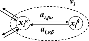

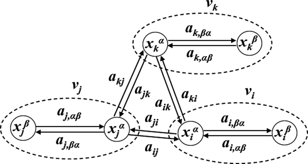


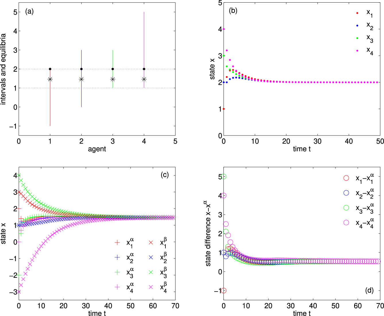


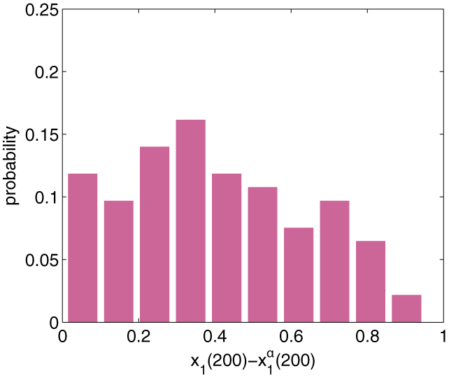


 Open access

