





1. Introduction
Prediction and control of particles in flows are important in a wide range of applications, in both natural and industrial contexts. For example, the climate and computational weather predictions of clouds containing ice hydrometeors are affected by the variation in shape and orientation of the hydrometeors (Duncan & Eriksson Reference Duncan and Eriksson2018). Other applications include flow predictions for the dispersion of pollen (Sabban & van Hout Reference Sabban and van Hout2011; Roy et al. Reference Roy, Chen, Chen, Ahmad, Khan and Buttner2023) or the transport of floating plastic on the ocean surface (Van Sebille et al. Reference Van Sebille2020; Sanness Salmon et al. Reference Sanness Salmon, Baker, Kozarek and Coletti2023). In an industrial context, particle-laden flows have applications in pharmaceutical processes (Erni et al. Reference Erni, Cramer, Marti, Windhab and Fischer2009) and in recycling processes (Pongstabodee et al. Reference Pongstabodee, Kunachitpimol and Damronglerd2008; Chan et al. Reference Chan, Blay Esteban, Huisman, Shrimpton and Ganapathisubramani2021). Particles in these flows are generally non-spherical, which lead to a large range of complicated linear and angular velocity dynamics (Voth & Soldati Reference Voth and Soldati2017). The non-spherical shape of these particles introduces orientation dependence of forces and torques on the suspended particles (Marchioli et al. Reference Marchioli2025). Besides the shape of the particles, the turbulence of the particle-laden flow provides rich and complex dynamics: the parameter space is spanned by the particle-to-fluid density ratio, particle size compared with the smallest turbulence scales, and the solid-phase volume fraction (Brandt & Coletti Reference Brandt and Coletti2022). Already on small scales, for laminar flow, the dynamics of falling non-spherical particles in still water is extremely rich and counter-intuitive (Joshi & Govindarajan Reference Joshi and Govindarajan2025).
In the context of studying ice hydrometeors, disks and perforated disks have been used to reproduce the settling dynamics of porous ice crystals and plates in a laboratory setting (Tinklenberg et al. Reference Tinklenberg, Guala and Coletti2025). The settling of millimetre-sized disks in quiescent air shows a bimodal distribution in falling modes, with disks either falling stably and aligned to the horizontal plane, or tumbling. However, the falling modes are non-trivially related to the particle size, with certain disk sizes displaying almost exclusively the tumbling falling mode (Tinklenberg et al. Reference Tinklenberg, Guala and Coletti2023). Introducing turbulence in this settling disk experiment significantly affects the settling dynamics for larger disks: the fall speed decreases for increasing disk size and turbulence strength, while the turbulence also causes the disks to tumble, leading to a more randomised orientation distribution. This being said, smaller disks (of sub-millimetre diameter) tend to fall aligned to the horizontal plane, regardless of the turbulence strength (Tinklenberg et al. Reference Tinklenberg, Guala and Coletti2024). Changing the disk shape by adding perforations affects the settling dynamics, where perforated disks are stabilised and tumble less frequently. In addition, the turbulence increases the drag coefficient for perforated disks through cross-flow-induced drag (Tinklenberg et al. Reference Tinklenberg, Guala and Coletti2025).
These results show that the shape, size and turbulence all significantly affect the settling dynamics of disks in non-trivial ways. Going beyond disks, rods and fibres show much different dynamics in turbulence compared with disks. Fibres show a higher variance of the spinning rate than that of the tumbling rate, indicating that fibres spin more than they tumble (Oehmke et al. Reference Oehmke, Bordoloi, Variano and Verhille2021), whereas disks tumble more than they spin, due to the different alignment with the fluid vorticity (Byron et al. Reference Byron, Einarsson, Gustavsson, Voth, Mehlig and Variano2015). The resulting mean square rotation rates for disks are much higher compared with spheres or rods (Parsa et al. Reference Parsa, Calzavarini, Toschi and Voth2012). The mean square tumbling rate of the rods was also found to scale as $\propto l^{-4/3}$
in the inertial range of turbulence, where
$\propto l^{-4/3}$
in the inertial range of turbulence, where $l$
is the rod length (Parsa & Voth Reference Parsa and Voth2014). A similar scaling exists for the variance of the spinning rate, which scales as
$l$
is the rod length (Parsa & Voth Reference Parsa and Voth2014). A similar scaling exists for the variance of the spinning rate, which scales as $\propto (d/\eta _K)^{-4/3}$
, with
$\propto (d/\eta _K)^{-4/3}$
, with $d$
the diameter of the fibre. For cylinders of small aspect ratio and spheroids, the mean square angular velocity was also shown to scale as
$d$
the diameter of the fibre. For cylinders of small aspect ratio and spheroids, the mean square angular velocity was also shown to scale as $l^{-4/3}$
in experiments and simulations, but here
$l^{-4/3}$
in experiments and simulations, but here $l$
was given by the volume-equivalent diameter (Bordoloi & Variano Reference Bordoloi and Variano2017; Jiang et al. Reference Jiang, Wang, Liu, Sun and Calzavarini2022). Once again, this illustrates the vast parameter space affecting the dynamics of anisotropic particles in turbulence, and emphasises that particle dynamics is affected by the particle’s shape, size and the ambient turbulence.
$l$
was given by the volume-equivalent diameter (Bordoloi & Variano Reference Bordoloi and Variano2017; Jiang et al. Reference Jiang, Wang, Liu, Sun and Calzavarini2022). Once again, this illustrates the vast parameter space affecting the dynamics of anisotropic particles in turbulence, and emphasises that particle dynamics is affected by the particle’s shape, size and the ambient turbulence.
This study focuses on an even wider class than symmetrical particles, namely on chiral particles, which break mirror symmetry. On the very smallest scales, chiral molecules have applications in chemistry (Roos & Roos Reference Roos and Roos2015), and many biological systems are often intrinsically chiral (Chan et al. Reference Chan, Blay Esteban, Huisman, Shrimpton and Ganapathisubramani2021). An example of a chiral particle is a maple seed, which autorotates as it descends, increasing its lift, thereby increasing the distance it can travel (Lentink et al. Reference Lentink, Dickson, Van Leeuwen and Dickinson2009; Sohn & Im Reference Sohn and Im2022). This translation–rotation coupling is further illustrated in recent work by Huseby et al. (Reference Huseby, Gissinger, Candelier, Pujara, Verhille, Mehlig and Voth2025), who use helical ribbons with a strong translation–rotation coupling. Settling these ribbons in a quiescent fluid at very low Reynolds numbers results in quasi-periodic angular dynamics and complex spatial trajectories. Here the helical ribbon length and the initial orientation strongly affect the dynamics and resulting trajectory.
Chiral particles in turbulence have been investigated by Kramel et al. (Reference Kramel, Voth, Tympel and Toschi2016), showing that a chiral dipole (a rod with two chiral ends) has a preferential rotation in homogeneous isotropic turbulence, resulting from an alignment of the particle with the fluid strain. More recently, Piumini et al. (Reference Piumini, Assen, Lohse and Verzicco2024) computationally investigated heavy chiral particles $ ( 2 \leqslant \rho _p/\rho _f \leqslant 10 )$
in quiescent fluid and homogeneous isotropic turbulence. In a quiescent fluid, the particles display a translation–rotation coupling, where the rotation direction is determined by the particle chirality. As the turbulence is increased, the chirality-induced mean rotation decreases, such that the chirality does not matter at high Reynolds numbers. Other studies have pointed out that the rotation direction of a particle is not solely determined by the inherent chirality of the particle (Moreno, Vázquez-Cortés & Fried Reference Moreno, Vázquez-Cortés and Fried2024).
$ ( 2 \leqslant \rho _p/\rho _f \leqslant 10 )$
in quiescent fluid and homogeneous isotropic turbulence. In a quiescent fluid, the particles display a translation–rotation coupling, where the rotation direction is determined by the particle chirality. As the turbulence is increased, the chirality-induced mean rotation decreases, such that the chirality does not matter at high Reynolds numbers. Other studies have pointed out that the rotation direction of a particle is not solely determined by the inherent chirality of the particle (Moreno, Vázquez-Cortés & Fried Reference Moreno, Vázquez-Cortés and Fried2024).
This study experimentally and theoretically studies the settling dynamics of heavy chiral particles in a quiescent fluid and in turbulence, employing the same chiral particles as used by Piumini et al. (Reference Piumini, Assen, Lohse and Verzicco2024). The particle geometries used here are illustrated in figure 1(a) and a photograph of the particles is shown in figure 1(b). The reference orientation of the particles is shown in figure 1(c), with the red arrow indicating the pointing vector. The pointing vector is defined with respect to the particle body coordinate system: it originates at the middle of the central rod (the origin of the coordinate system) and passes through the centre of mass (vertically above the origin). Thereby, the pointing vector perfectly dissects the angle made by the inclined rods in the $y,z$
plane. The particles consist of three equally large rods, all being mutually orthogonal. This allows for two different particle chiralities, giving left-handed and right-handed particles. The particle geometry (assuming unit length) as seen in figure 1(c) can be defined more exactly as a cylindrical tube running through the points
$y,z$
plane. The particles consist of three equally large rods, all being mutually orthogonal. This allows for two different particle chiralities, giving left-handed and right-handed particles. The particle geometry (assuming unit length) as seen in figure 1(c) can be defined more exactly as a cylindrical tube running through the points $(1/2,1/\sqrt {2}, 1/\sqrt {2}), (1/2,0,0),(-1/2,0,0),(-1/2,-1/\sqrt {2},1/\sqrt {2})$
, with hemispherical end caps centred at the listed end points. The geometry of the right-handed particle is obtained by a reflection in the
$(1/2,1/\sqrt {2}, 1/\sqrt {2}), (1/2,0,0),(-1/2,0,0),(-1/2,-1/\sqrt {2},1/\sqrt {2})$
, with hemispherical end caps centred at the listed end points. The geometry of the right-handed particle is obtained by a reflection in the $x,z$
plane. This specific particle shape was chosen due its simplicity, while still breaking mirror symmetry.
$x,z$
plane. This specific particle shape was chosen due its simplicity, while still breaking mirror symmetry.
(a) A 3D visualisation of a chiral enantiomorph, displaying a left-handed and right-handed particle. (b) A photograph of the three-dimensionally printed chiral particles used in experiments. (c) A 3D visualisation of a chiral particle in its reference orientation, including axes, and a pointing vector shown by the red arrow.

We also compare and contrast the findings of chiral particles in turbulence with previously found computational results. We aim to characterise the dynamics of settling chiral particles in a quiescent flow and illustrate any differences in dynamics caused by the particle chirality. By introducing and increasing turbulence in the settling dynamics, we highlight how the particle dynamics change as a result of the turbulence strength. Based on these results, we can conclude whether any difference in dynamics between the particle chiralities vanish at high turbulence intensity, as seen computationally.
The paper is organised as follows. Section 2 shows the experimental set-up used to perform the experiments and characterises the turbulent flow used for the settling experiments. Furthermore, this section uses a simple model to obtain a first estimate of the particle’s settling velocity and angular velocity. Section 3 describes the results and compares findings from the present study to previous computational work. Section 4 presents a simple theoretical model for particle settling that incorporates the effect of turbulence with stochastic forcing. We use this model to clarify our experimental findings. Finally, § 5 provides concluding remarks and an outlook.
2. Experimental set-up
The particles used in the settling experiments are three-dimensionally printed using a Formlabs Form 3 printer. Figure 1(b) shows the chiral particles, which have a characteristic size of $l =$
11.3 mm (the length of one straight line segment of the particle, termed a ‘rod’ of the particle), or an end-to-end Euclidean length of approximately 17 mm, and a density of
$l =$
11.3 mm (the length of one straight line segment of the particle, termed a ‘rod’ of the particle), or an end-to-end Euclidean length of approximately 17 mm, and a density of $\rho =$ ${1.30 \times 10^3}\,\mathrm{kg\,m}^{-3}$
. The diameter of each rod is
${1.30 \times 10^3}\,\mathrm{kg\,m}^{-3}$
. The diameter of each rod is $d =$
3.2 mm. We let the particles settle in our dodecahedron set-up (henceforth, simply termed the ‘dodecahedron’), which is shown in figure 2(a) and is based on the Lagrangian exploration module (LEM) set-up described by Zimmermann et al. (Reference Zimmermann, Xu, Gasteuil, Bourgoin, Volk, Pinton and Bodenschatz2010). The dodecahedron has edge lengths of 30 cm and a total volume of approximately
$d =$
3.2 mm. We let the particles settle in our dodecahedron set-up (henceforth, simply termed the ‘dodecahedron’), which is shown in figure 2(a) and is based on the Lagrangian exploration module (LEM) set-up described by Zimmermann et al. (Reference Zimmermann, Xu, Gasteuil, Bourgoin, Volk, Pinton and Bodenschatz2010). The dodecahedron has edge lengths of 30 cm and a total volume of approximately $V =$
210L. For these experiments, the dodecahedron is filled with water. The set-up is equipped with 20 engines (Beckhoff AM8033), which have a maximum power of 1 kW each. Each engine rotates a three-dimensionally printed toroidal propeller, shown in figure 2(b). The propeller’s shape causes the fluid displacement to differ substantially depending on the direction in which it rotates. This is further shown in § 2.1, where we characterise the flow in the dodecahedron using laser Doppler anemometry (LDA).
$V =$
210L. For these experiments, the dodecahedron is filled with water. The set-up is equipped with 20 engines (Beckhoff AM8033), which have a maximum power of 1 kW each. Each engine rotates a three-dimensionally printed toroidal propeller, shown in figure 2(b). The propeller’s shape causes the fluid displacement to differ substantially depending on the direction in which it rotates. This is further shown in § 2.1, where we characterise the flow in the dodecahedron using laser Doppler anemometry (LDA).
(a) A render of the dodecahedron set-up, including a definition of the lab coordinate axes, where the origin is at the centre of the set-up. (b) A 3D drawing of one of the toroidal propellers used inside the dodecahedron. The blue arrow indicates the axis of rotation and the red arrow shows the positive rotation direction.

To perform the settling experiments, the chiral particles were released in water one-by-one at the top of the dodecahedron. We released the particles by hand, with a random initial orientation, approximately 55 cm above the centre of the set-up, such that the particles reach their terminal velocity in the measurement volume. The particles were tracked in the centre of the set-up, where we used a single Photron Nova S16 and two Photron Mini AX-200 high-speed cameras (all 1024 $\times$
1024 px) to record the settling particles. Two cameras are mounted to the large windows on the front of the set-up, while the third camera is mounted on the smaller window on top. The cameras image a measurement volume of approximately 10
$\times$
1024 px) to record the settling particles. Two cameras are mounted to the large windows on the front of the set-up, while the third camera is mounted on the smaller window on top. The cameras image a measurement volume of approximately 10 $\times$
19
$\times$
19 $\times$
15 cm, with a resolution of approximately
$\times$
15 cm, with a resolution of approximately ${160}\,{\unicode[Arial]{x0B5}}\mathrm{ m \, (px)}^{-1}$
for the cameras on the front windows, while the top camera has a resolution of approximately
${160}\,{\unicode[Arial]{x0B5}}\mathrm{ m \, (px)}^{-1}$
for the cameras on the front windows, while the top camera has a resolution of approximately ${175}\,{\unicode[Arial]{x0B5}}\mathrm{ m \, (px)}^{-1}$
. All cameras record using a frame rate of 250fps.
${175}\,{\unicode[Arial]{x0B5}}\mathrm{ m \, (px)}^{-1}$
. All cameras record using a frame rate of 250fps.
The particles are tracked using the orientation tracking algorithm described in Flapper et al. (Reference Flapper, Bernard and Huisman2025), specifically designed for tracking the orientation of anisotropic particles, where the algorithm can distinguish the particle chirality. This method creates a synthetic particle with a known orientation and calculates the synthetic projections seen by the cameras. The synthetic particle projections are compared with the experimental images, and the synthetic particle’s orientation is varied to minimise the difference between experimental images and synthetic projections. The resulting orientation of the synthetic particle then gives the orientation of the experimentally imaged particle. A three-dimensional (3D) chiral particle is then reconstructed by using the found orientation. An example of a recorded image and the reconstructed particle is shown in figure 3. An animation of a recorded video alongside the reconstructed particles is shown in movie 1 of the supplementary material available at https://doi.org/10.1017/jfm.2026.11726.
A raw image of a recorded chiral particle (a), and its corresponding 3D reconstruction (b). The method for reconstructing the particle is described in Flapper et al. (Reference Flapper, Bernard and Huisman2025).

To investigate the effect of turbulence on the settling dynamics, the Reynolds number was varied by rotating the propellers at different rotation rates: the propellers were rotated at 0, −0.25, −0.5, −1, −2 and −4 Hz, with all propellers rotating in the same direction at the same rotation rate. The highest absolute rotation rate of −4 Hz was chosen due to it being the highest absolute rotation rate where the particles still sank. The flow generated by this set-up was characterised using LDA to find the resulting flow parameters such as the velocity fluctuations, isotropy, energy dissipation rate and the Taylor–Reynolds number. The findings and results from these measurements are detailed below.
2.1. Turbulent flow characterisation
Using LDA, the $y$
component and
$y$
component and $z$
component of the velocity (
$z$
component of the velocity ( $u$
and
$u$
and $v$
, respectively) are measured in the centre of the dodecahedron. We record velocity time series for absolute rotation rates between 1 and 20 Hz in both rotation directions. The lower bound of 1 Hz was used since the lower propeller rotation speed resulted in too low velocity fluctuations to be measured reliably. Each measurement collects data for 30 min, in which the propellers rotate at a constant frequency. The collected velocity data are used to calculate the standard deviations in velocity
$v$
, respectively) are measured in the centre of the dodecahedron. We record velocity time series for absolute rotation rates between 1 and 20 Hz in both rotation directions. The lower bound of 1 Hz was used since the lower propeller rotation speed resulted in too low velocity fluctuations to be measured reliably. Each measurement collects data for 30 min, in which the propellers rotate at a constant frequency. The collected velocity data are used to calculate the standard deviations in velocity $\sigma (u)$
and
$\sigma (u)$
and $\sigma (v)$
for each rotation frequency, the ratio of which indicates the isotropy of the flow. Figure 4 shows this plot, illustrating the standard deviations in both velocity components. Again, we note that the difference between the positive and negative rotation frequency is caused by the propeller shape: the negative rotation frequencies ‘push’ the fluid towards the centre of the dodecahedron, while the positive rotation frequencies ‘pull’ the fluid from the centre. For the negative rotation frequencies (‘pushing’ the fluid), the ratio of velocity standard deviations is around
$\sigma (v)$
for each rotation frequency, the ratio of which indicates the isotropy of the flow. Figure 4 shows this plot, illustrating the standard deviations in both velocity components. Again, we note that the difference between the positive and negative rotation frequency is caused by the propeller shape: the negative rotation frequencies ‘push’ the fluid towards the centre of the dodecahedron, while the positive rotation frequencies ‘pull’ the fluid from the centre. For the negative rotation frequencies (‘pushing’ the fluid), the ratio of velocity standard deviations is around $\sigma (u)/\sigma (v) = 4/5$
, whereas the positive rotation frequencies are all in the range
$\sigma (u)/\sigma (v) = 4/5$
, whereas the positive rotation frequencies are all in the range $ 0.93 \leqslant \sigma (u)/\sigma (v) \leqslant 1.11$
. This indicates better isotropy when pulling the fluid, compared with pushing. Looking at the values of the standard deviation in both velocity components, we observe that the absolute values are consistently higher for pushing compared with pulling, indicating a higher turbulence strength for pushing.
$ 0.93 \leqslant \sigma (u)/\sigma (v) \leqslant 1.11$
. This indicates better isotropy when pulling the fluid, compared with pushing. Looking at the values of the standard deviation in both velocity components, we observe that the absolute values are consistently higher for pushing compared with pulling, indicating a higher turbulence strength for pushing.
Standard deviation in the horizontal and vertical velocity components plotted against one another for numerous propeller rotation frequencies. Added lines indicate ratios between the velocity standard deviations.

For the homogeneity of the turbulent flow, we rely on the study by Zimmermann et al. (Reference Zimmermann, Xu, Gasteuil, Bourgoin, Volk, Pinton and Bodenschatz2010) on the very similar LEM. The flow in the LEM is homogeneous, as shown by extensive particle tracking measurements. The dodecahedron set-up used in this study is of similar design, and has more engines (20 vs 12). Since the 20 engines provide a more isotropic distribution of the engines (a higher ‘sphericity’), we expect a similar homogeneity for the flow in the dodecahedron.
Characterising the strength of the turbulence is done by calculating the energy dissipation rate $\epsilon$
, computed from the second-order structure function. Employing the Kolmogorov hypotheses for large
$\epsilon$
, computed from the second-order structure function. Employing the Kolmogorov hypotheses for large $r$
in the inertial range
$r$
in the inertial range $(\eta \lt r \lt L)$
, the relation between the longitudinal structure function and the energy dissipation rate is given by (assuming no intermittency corrections)
$(\eta \lt r \lt L)$
, the relation between the longitudinal structure function and the energy dissipation rate is given by (assuming no intermittency corrections)
 \begin{align} D_{\textit{LL}}(r) = C_2 (\epsilon r)^{2/3}. \end{align}
Here $D_{\textit{LL}}$
is the longitudinal structure function,
$D_{\textit{LL}}$
is the longitudinal structure function, $r$
is the distance between two points and
$r$
is the distance between two points and $C_2 = 2.0$
is a universal constant (Pope Reference Pope2017). From this equation, the energy dissipation rate can be calculated as
$C_2 = 2.0$
is a universal constant (Pope Reference Pope2017). From this equation, the energy dissipation rate can be calculated as
 \begin{align} \epsilon = \frac {1}{r} \left (\frac {D_{\textit{LL}}(r)}{C_2} \right )^{3/2}, \end{align}
which can be estimated by finding a plateau of the compensated structure function in the inertial range. Since the LDA probes a single position over a long period of time, the separation in time is converted to a separation in space by using the measured velocity and the difference in arrival time (Buchhave & Velte Reference Buchhave and Velte2017). Figure 5 shows the calculated values of the energy dissipation rate for the measured propeller frequencies on a logarithmic plot. The colour of the points show the rotation direction of the propeller. The black triangle shows the expected cubic scaling between the energy dissipation rate and the propeller rotation frequency, where the measurements follow the expected scaling well.
The energy dissipation rate $\epsilon$
as a function of the propeller rotation frequency. The black triangle shows the expected cubic scaling between the energy dissipation rate and the frequency.
$\epsilon$
as a function of the propeller rotation frequency. The black triangle shows the expected cubic scaling between the energy dissipation rate and the frequency.

For the settling experiments reported below, propeller rotation rates from 0 to −4 Hz are used, where we choose to use negative rotation rates due to the higher energy dissipation rate, despite higher anisotropy. The most important flow parameters at the various rotation rates are displayed in table 1. The reported values are based on the measured longitudinal structure function and the resulting values of $\epsilon$
, where the data for the rotation rates lower than 1 Hz are extrapolated from the measured data. The ambient turbulence is characterised by the Taylor–Reynolds number, given by
$\epsilon$
, where the data for the rotation rates lower than 1 Hz are extrapolated from the measured data. The ambient turbulence is characterised by the Taylor–Reynolds number, given by
 \begin{align} \textit{Re}_{\lambda } = \frac {\sigma (v)\lambda }{\nu } \text{,} \end{align}
where $\lambda = \sigma (v)\sqrt {15 \nu /\epsilon }$
is the Taylor length and
$\lambda = \sigma (v)\sqrt {15 \nu /\epsilon }$
is the Taylor length and $\nu$
is the kinematic viscosity. The particle Reynolds number
$\nu$
is the kinematic viscosity. The particle Reynolds number $\textit{Re}_{\textit{p}}$
is computed as
$\textit{Re}_{\textit{p}}$
is computed as
 \begin{align} \textit{Re}_{\textit{p}} = \frac {(\epsilon l)^{1/3} l}{\nu }, \end{align}
where we have used $(\epsilon l)^{1/3}$
as a relevant velocity scale at the particle scale. Similarly, the Stokes number is defined as
$(\epsilon l)^{1/3}$
as a relevant velocity scale at the particle scale. Similarly, the Stokes number is defined as
 \begin{align} \textit{Stk} = \frac {l^{2/3}\epsilon ^{-1/3}}{\tau _K} \text{,} \end{align}
with $l^{2/3}\epsilon ^{-1/3}$
representing the time scale at the size of the particle and
$l^{2/3}\epsilon ^{-1/3}$
representing the time scale at the size of the particle and $\tau _K$
is the Kolmogorov time scale. The Kolmogorov time scale and length scale are respectively given by
$\tau _K$
is the Kolmogorov time scale. The Kolmogorov time scale and length scale are respectively given by $\tau _K = \sqrt {{\nu }/{\epsilon }}$
and
$\tau _K = \sqrt {{\nu }/{\epsilon }}$
and $\eta _K = ( {\nu ^3}/{\epsilon } )^{1/4}$
. With this, we also compute the ratio between the particle length scale
$\eta _K = ( {\nu ^3}/{\epsilon } )^{1/4}$
. With this, we also compute the ratio between the particle length scale $l$
and the Kolmogorov length scale
$l$
and the Kolmogorov length scale $\eta _K$
. Notably, the chiral particles are always larger than the Kolmogorov length scale. Finally, we compute the integral length scale
$\eta _K$
. Notably, the chiral particles are always larger than the Kolmogorov length scale. Finally, we compute the integral length scale $L$
, defined as
$L$
, defined as
 \begin{align} L = \frac {C_L\sigma (v)^3}{\epsilon }, \end{align}
where $C_L$
is a dimensionless constant, taken as
$C_L$
is a dimensionless constant, taken as $C_L = 1$
, similar to the definition used in Zimmermann et al. (Reference Zimmermann, Xu, Gasteuil, Bourgoin, Volk, Pinton and Bodenschatz2010). Besides the flow conditions listed in table 1, we also performed an experiment in quiescent water. For the quiescent settling case, the most relevant parameter is the Galileo number, given by
$C_L = 1$
, similar to the definition used in Zimmermann et al. (Reference Zimmermann, Xu, Gasteuil, Bourgoin, Volk, Pinton and Bodenschatz2010). Besides the flow conditions listed in table 1, we also performed an experiment in quiescent water. For the quiescent settling case, the most relevant parameter is the Galileo number, given by
 \begin{align} \textit{Ga} = \frac {l \sqrt {g l \left (\frac {\rho _p}{\rho _f} - 1 \right )}}{\nu }, \end{align}
resulting in a value of $\textit{Ga} = 2.1\times 10^3$
.
$\textit{Ga} = 2.1\times 10^3$
.
Turbulent flow parameters.

Settling measurements were performed in quiescent water and in each of the turbulent flows reported in table 1. For each measurement, approximately 90 particles of each chirality were tracked while settling.
3. Results
We track the settling chiral particles, measuring their position and orientation over time. The linear and angular velocities of the particles are obtained through time differentiation of these results. This procedure is performed across a range of Reynolds numbers. An overview of the general results is illustrated in figure 6, showing snapshots of settling chiral particles (all left-handed) in flows of the various measured turbulence levels. The snapshots are all spaced by 0.14s, and the blue line shows the centre-of-mass trajectory, whereas the red arrow represents the pointing vector as defined in figure 1(c). An animated version of this figure is shown in movie 2 of the supplementary material, which more clearly illustrates the particle dynamics. The figure shows that the particle aligns with its pointing vector opposing the direction of gravity for a small Taylor–Reynolds number, though the alignment weakens as the turbulence increases. Similarly, we can see a clear preferential rotation around the vertical when studying the snapshots, which demonstrates a translation–rotation coupling. Again, this preferential rotation vanishes when increasing the Reynolds numbers. Finally, the horizontal movement of the particle is observed to increase with the turbulence intensity. Overall, we see the transition from a stable settling mode, with clear alignment and rotation, to a more irregular falling mode (tumbling) as the turbulence is increased. The same observations are made when examining right-handed particles, where only the rotation direction around the vertical is reversed. These observations are studied in more detail in the following sections.
Snapshots of settling chiral particles at the different turbulence levels. All shown particles are left-handed, with snapshots spaced 0.14 s apart. The blue line shows the centre-of-mass trajectory and the red arrow indicates the pointing vector.

Particle Reynolds number based on the settling velocity as a function of the Taylor–Reynolds number.

The mean settling velocity in the vertical direction is calculated per particle, and averaged per Taylor–Reynolds number, where each particle’s velocity is weighted by the duration of the recorded trajectories. The mean settling velocity $\langle v_z \rangle$
is then non-dimensionalised and, thus, expressed as a particle Reynolds number
$\langle v_z \rangle$
is then non-dimensionalised and, thus, expressed as a particle Reynolds number $\textit{Re}_{\textit{z}}$
, defined as
$\textit{Re}_{\textit{z}}$
, defined as $\langle v_z \rangle l / \nu$
, using the characteristic rod length
$\langle v_z \rangle l / \nu$
, using the characteristic rod length $l$
and the kinematic viscosity
$l$
and the kinematic viscosity $\nu$
. This particle Reynolds number is plotted against the Taylor–Reynolds number,
$\nu$
. This particle Reynolds number is plotted against the Taylor–Reynolds number, $\textit{Re}_\lambda$
, in figure 7. The interval markers show a standard deviation in the average settling velocity (non-dimensionalised into
$\textit{Re}_\lambda$
, in figure 7. The interval markers show a standard deviation in the average settling velocity (non-dimensionalised into $\textit{Re}_{\textit{z}}$
). The plot illustrates that the average settling velocity is not strongly affected at low Taylor–Reynolds numbers, but the variation in velocity increases with the Taylor–Reynolds number. Only for the highest Taylor–Reynolds number do we see a large decrease in average settling velocity. For this data point, the standard deviation is very large, which is due to the large velocity fluctuations with respect to the quiescent falling velocity. The overall finding from this plot is in agreement with previous studies, which found a reduction in settling velocity for heavy anisotropic particles as a result of turbulence (Good & et al. Reference Good2014; Chan et al. Reference Chan, Blay Esteban, Huisman, Shrimpton and Ganapathisubramani2021; Tinklenberg et al. Reference Tinklenberg, Guala and Coletti2024).
$\textit{Re}_{\textit{z}}$
). The plot illustrates that the average settling velocity is not strongly affected at low Taylor–Reynolds numbers, but the variation in velocity increases with the Taylor–Reynolds number. Only for the highest Taylor–Reynolds number do we see a large decrease in average settling velocity. For this data point, the standard deviation is very large, which is due to the large velocity fluctuations with respect to the quiescent falling velocity. The overall finding from this plot is in agreement with previous studies, which found a reduction in settling velocity for heavy anisotropic particles as a result of turbulence (Good & et al. Reference Good2014; Chan et al. Reference Chan, Blay Esteban, Huisman, Shrimpton and Ganapathisubramani2021; Tinklenberg et al. Reference Tinklenberg, Guala and Coletti2024).
The overall particle velocity is in the downward direction, though the particle velocity in the horizontal plane increases with turbulence. This is evident from studying the top view of the particle trajectories, shown in figure 8(a). This plot shows a number of projected trajectories for all measured turbulence levels, with all trajectories measured over the same time duration. The trajectories show an increase in traversed horizontal distance with increasing turbulence, which is further illustrated and quantified by computing the effective diffusion constants for the different Taylor–Reynolds numbers in Appendix A. In figure 8(b) the particle Reynolds number is computed using the root mean square of the horizontal velocity of the settling particles, where the error bars represent a standard deviation. The plot clearly illustrates an increase in the horizontal particle velocity and its variation as the turbulence intensity increases. We expect two effects to be relevant in figure 8(b): the wake effects of the particle are expected to cause significant horizontal motion, as observed for spheres (Uhlmann & Dušek Reference Uhlmann and Dušek2014; Uhlmann & Doychev Reference Uhlmann and Doychev2014), and the increasing turbulent forcing. We speculate that such wake effects cause the plateau for $\textit{Re}_\lambda \leqslant 50$
, after which the horizontal motions become dominated by the turbulent forcing. The results so far highlight a decrease in settling velocity and an increase in horizontal velocity as the turbulence strength increases, i.e. due to velocity fluctuations in the base flow generated by the propellers. Besides these effects of the turbulence on the translation of the particles, our main interests are in the particle orientation dynamics and how these are affected by the imposed turbulence.
$\textit{Re}_\lambda \leqslant 50$
, after which the horizontal motions become dominated by the turbulent forcing. The results so far highlight a decrease in settling velocity and an increase in horizontal velocity as the turbulence strength increases, i.e. due to velocity fluctuations in the base flow generated by the propellers. Besides these effects of the turbulence on the translation of the particles, our main interests are in the particle orientation dynamics and how these are affected by the imposed turbulence.
(a) Top view of the trajectories of a selection of the chiral particles for all measured turbulence levels. The trajectories have been shifted to start at the origin, all shown trajectories are taken over the same time span. (b) The particle Reynolds numbers based on the root mean square of the horizontal velocity. Error bars denote the standard deviation.

3.1. Orientation data
The reconstructed chiral particles allow us to closely study the orientation dynamics. First, we investigate whether the particles preferentially align as found by Piumini et al. (Reference Piumini, Assen, Lohse and Verzicco2024), and how any preferential alignment is affected by the turbulence. Computing the particle’s alignment is done by finding the pointing vector over time, where the pointing vector is chosen as shown in figure 1(c). The angle between the pointing vector and the vertical is then computed to find the alignment between the particle and the direction of gravity. The collected results of the alignment angle are shown in figure 9, which shows the probability density function (PDF) of the alignment angle for the different Reynolds numbers. The definition of the alignment angle is shown by the graphic on the right. Here we note that the particle’s rotation around the pointing vector is immaterial. The dashed line in the figure illustrates the curve for a randomly distributed orientation for reference. The PDFs of the alignment angle show a clear preferential alignment, as shown by the large deviation with respect to the random distribution: the pointing vector preferentially aligns opposite to the direction of gravity, as was also observed in numerical work by Piumini et al. (Reference Piumini, Assen, Lohse and Verzicco2024). This preferential alignment is visible for the lower Reynolds numbers and significantly weakens for the high Reynolds numbers. At the highest measured Reynolds numbers, the particle orientation is therefore no longer determined by the geometry of the particle, but rather by the imposed turbulent flow. This figure therefore illustrates a preferential alignment of the particle, which significantly weakens for increasing turbulence strength.
Probability density functions of the angle between the particle pointing vector and the vertical for all measured Reynolds numbers. The black dashed line indicates a random distribution. The graphic on the right shows the definition of the alignment angle.

3.2. Rotation data
Similar to the alignment of the particle’s pointing vector, we find the alignment of the rotation vector with respect to the vertical. The PDF of the angle between the rotation vector with the vertical is shown in figure 10, where the data are split between the left-handed and right-handed particles. Figure 10(a) shows that the left-handed particles preferentially have their rotation vector pointing in the direction of gravity, opposing the particles’ pointing vector. On the other hand, figure 10(b) illustrates that the right-handed particles have their rotation vector pointing opposite to the direction of gravity, aligning with the particles’ pointing vector. Comparing these results emphasises that the particle chirality dictates the rotation direction during settling, highlighting the translation–rotation coupling for these particles. This experimental finding is consistent with the numerical observations by Piumini et al. (Reference Piumini, Assen, Lohse and Verzicco2024), showing a difference in rotation direction for the left-handed and right-handed particles.
The PDF of the angle between the rotation vector and the vertical for (a) left-handed particles and (b) right-handed particles.

Comparing the rotation vector alignment across the measured Taylor–Reynolds numbers, $\textit{Re}_\lambda$
, we find that the preferential rotation becomes less pronounced as the Taylor–Reynolds number increases. For the highest Taylor–Reynolds numbers, no preferential rotation can be distinguished and the effect of the particle chirality on its rotation statistics vanishes, which is in line with the previous numerical simulations by Piumini et al. (Reference Piumini, Assen, Lohse and Verzicco2024).
$\textit{Re}_\lambda$
, we find that the preferential rotation becomes less pronounced as the Taylor–Reynolds number increases. For the highest Taylor–Reynolds numbers, no preferential rotation can be distinguished and the effect of the particle chirality on its rotation statistics vanishes, which is in line with the previous numerical simulations by Piumini et al. (Reference Piumini, Assen, Lohse and Verzicco2024).
3.3. Multiple settling modes
Besides the stable and tumbling settling mode illustrated in figure 6, another settling mode is observed, though rarely, in experiments. In contrast, in the numerical work, only the previously shown stable settling mode at low Reynolds numbers and a tumbling motion at higher Reynolds numbers was found.
We call this new mode the ‘corkscrew’ mode. The corkscrew mode is illustrated alongside the stable and tumbling mode in figure 11, showing snapshots of the different falling dynamics side by side. An animated version of this figure is shown in movie 3 in the supplementary material, showing the dynamics of the different settling modes more clearly. This figure shows the clear difference in orientation between the stable and corkscrew modes, even though both modes rotate around the vertical axis, and have a straight, vertical trajectory. In contrast, the tumbling mode does not show a clear alignment or rotation.
Snapshots of all observed falling modes of the chiral particles (all left-handed). The snapshots are separated by 0.14s, the blue line represents the centre-of-mass trajectory and the red arrow illustrates the pointing vector. The snapshots are all taken from measurements at $\textit{Re}_\lambda = 0$
.
$\textit{Re}_\lambda = 0$
.

These three experimentally found settling modes are studied in detail by examining the rotation angles of the particle over time for both particle chiralities, cf. figure 12. The plots show the particle’s rotation around the $x,y$
and
$x,y$
and $z$
axes with respect to the reference orientation shown in figure 1(c). Here
$z$
axes with respect to the reference orientation shown in figure 1(c). Here $\alpha$
gives the rotation around the
$\alpha$
gives the rotation around the $x$
axis,
$x$
axis, $\beta$
around the
$\beta$
around the $y$
axis and
$y$
axis and $\gamma$
around the
$\gamma$
around the $z$
axis, with the order of rotations
$z$
axis, with the order of rotations $x,y,z$
. The stable settling mode is characterised, as noted previously, by the rotation around the vertical axis, as illustrated by the angle
$x,y,z$
. The stable settling mode is characterised, as noted previously, by the rotation around the vertical axis, as illustrated by the angle $\gamma$
decreasing monotonically for the left-handed particle. The angles
$\gamma$
decreasing monotonically for the left-handed particle. The angles $\alpha$
and
$\alpha$
and $\beta$
oscillate around
$\beta$
oscillate around $0$
, indicating that the pointing vector oscillates closely around the vertical, as seen in figure 9 for low Taylor–Reynolds numbers. On the other hand, the right-handed particle shows a similar profile, though
$0$
, indicating that the pointing vector oscillates closely around the vertical, as seen in figure 9 for low Taylor–Reynolds numbers. On the other hand, the right-handed particle shows a similar profile, though $\gamma$
now increases monotonically, highlighting the differing rotation direction as a result of the particle chirality.
$\gamma$
now increases monotonically, highlighting the differing rotation direction as a result of the particle chirality.
The rotation angles over time for all observed falling modes, and both particle chiralities. The left-handed particles and right-handed particles are shown in the left column and right column, respectively. The rows display the stable, corkscrew and tumbling modes, respectively. The rotations are with respect to the reference orientation, with the $x$
,
$x$
, $y$
and
$y$
and $z$
axes as rotation axes (in this order). Here
$z$
axes as rotation axes (in this order). Here $\alpha$
,
$\alpha$
, $\beta$
and
$\beta$
and $\gamma$
denote the rotations around the
$\gamma$
denote the rotations around the $x$
,
$x$
, $y$
and
$y$
and $z$
axes, respectively.
$z$
axes, respectively.

The ‘corkscrew’ mode is remarkable due to the particle rotating around the $z$
axis in the opposite direction compared with the regular stable falling mode, as
$z$
axis in the opposite direction compared with the regular stable falling mode, as $\gamma$
now increases monotonically for the left-handed particle. We note that the rotation angles
$\gamma$
now increases monotonically for the left-handed particle. We note that the rotation angles $\alpha$
and
$\alpha$
and $\beta$
oscillate little and are not centred around
$\beta$
oscillate little and are not centred around $0$
. The angle
$0$
. The angle $\alpha$
is close to
$\alpha$
is close to $-\pi /2$
, indicating that the pointing vector (approximately) lies in the
$-\pi /2$
, indicating that the pointing vector (approximately) lies in the $x,y$
plane. This is in contrast to the stable falling mode, where the pointing vector aligns opposite to gravity. Again, the right-handed particle shows similar rotation angles with a reversed rotation direction around the
$x,y$
plane. This is in contrast to the stable falling mode, where the pointing vector aligns opposite to gravity. Again, the right-handed particle shows similar rotation angles with a reversed rotation direction around the $z$
axis. A last point worth noting is that the angular velocity of the corkscrew is slightly higher compared with the stable settling mode:
$z$
axis. A last point worth noting is that the angular velocity of the corkscrew is slightly higher compared with the stable settling mode: $\omega =$
10 rad s−1 for the corkscrew mode compared with
$\omega =$
10 rad s−1 for the corkscrew mode compared with $\omega =$
7 rad s−1 for the stable settling chiral particles. Finally, the tumbling mode displays a more random orientation over time. The orientation angles show no clear pattern, nor periodicity.
$\omega =$
7 rad s−1 for the stable settling chiral particles. Finally, the tumbling mode displays a more random orientation over time. The orientation angles show no clear pattern, nor periodicity.
These different settling modes are tallied to evaluate their frequency of occurrence. Using a $k$
-means clustering algorithm, each particle track is classified as stable, corkscrew or tumbling. This classification is done based on 12 parameters per particle track: for each rotation angle, we compute the mean, slope, linear fit residuals and standard deviation of the residuals. The clustering is applied to particle tracks longer than
$k$
-means clustering algorithm, each particle track is classified as stable, corkscrew or tumbling. This classification is done based on 12 parameters per particle track: for each rotation angle, we compute the mean, slope, linear fit residuals and standard deviation of the residuals. The clustering is applied to particle tracks longer than $100$
frames, which we find to give a good indication of the settling mode. The clusters are checked manually and corrected where necessary: the size of the clusters indicate how frequently each settling mode occurs at each turbulence level. This is shown in figure 13, indicating how often each settling mode occurs in percentages. The data are split by particle chirality and the numbers above the bars indicate how many particles are tracked for each Taylor–Reynolds number (split by particle chirality). This affirms earlier findings, emphasising the common occurrence of the stable settling mode at lower turbulence levels, which becomes rarer as the turbulence increases. The fact that settling modes besides tumbling are still observed at large Taylor–Reynolds numbers indicates that preferential alignment and rotation can still occur at surprisingly high turbulence strengths. Another point we observe is that the corkscrew settling mode only occurs rarely: based on the rare occurrence, and the absence of this settling mode in numerical simulations, the cause for this settling mode cannot be readily identified from the obtained results.
$100$
frames, which we find to give a good indication of the settling mode. The clusters are checked manually and corrected where necessary: the size of the clusters indicate how frequently each settling mode occurs at each turbulence level. This is shown in figure 13, indicating how often each settling mode occurs in percentages. The data are split by particle chirality and the numbers above the bars indicate how many particles are tracked for each Taylor–Reynolds number (split by particle chirality). This affirms earlier findings, emphasising the common occurrence of the stable settling mode at lower turbulence levels, which becomes rarer as the turbulence increases. The fact that settling modes besides tumbling are still observed at large Taylor–Reynolds numbers indicates that preferential alignment and rotation can still occur at surprisingly high turbulence strengths. Another point we observe is that the corkscrew settling mode only occurs rarely: based on the rare occurrence, and the absence of this settling mode in numerical simulations, the cause for this settling mode cannot be readily identified from the obtained results.
Percentage of occurrence for each falling modes, shown for all measured Taylor–Reynolds numbers, split between particle chirality. The numbers above the bar chart indicate the number of tracked left-handed and right-handed particles.

The absence of the corkscrew settling mode in simulations calls for extra investigation: computationally, different initial orientations were explored, which were unable to produce the corkscrew mode. Experimentally, extra measurements were performed, which showed that the corkscrew mode is likely to occur when a bubble is attached to the end of a chiral particle, which leads to a distorted density distribution. Therefore, it seems likely that an experimental artefact or perturbation is the cause for the corkscrew mode. Along similar lines, previous studies have shown that small perturbations or asymmetries can have large effects on a particle’s settling dynamics and can lead to settling modes unobserved for perfectly symmetrical particles (Moths & Witten Reference Moths and Witten2013; Roy et al. Reference Roy, Hamati, Tierney, Koch and Voth2019). An experimental artefact or asymmetry could therefore be the cause for the remarkably stable corkscrew mode, which is observed across all measured Taylor–Reynolds numbers. To be able to control such asymmetries, in the next section we introduce a theoretical model for a chiral particle settling in Stokes flow. In this model, we can accurately control initial conditions and carefully introduce controlled asymmetries in the mass distributions of the particle and study their effects.
4. Theoretical model
To clarify and further investigate the chiral particle’s settling dynamics, we develop a model based on a simplified chiral particle consisting of four rigidly connected spheres, as shown in figure 14. This replaces the true particle geometry with a minimal set of spheres that are chosen to capture the chiral particle’s symmetry and its dominant fluid-structure physics. The settling dynamics of this particle, assuming a Stokes flow under gravity, are calculated using standard hydrodynamics that employs the Oseen mobility tensor to account for the hydrodynamic coupling between the spheres. This enables the velocity of each sphere to be calculated provided spheres are well separated relative to their radii: in our case the separation length is unity, whereas the radii of the spheres is $1/10$
. The spheres are centred at the points
$1/10$
. The spheres are centred at the points $(1/2,1/\sqrt {2}, 1/\sqrt {2}), (1/2,0,0),(-1/2,0,0),(-1/2,-1/\sqrt {2},1/\sqrt {2})$
. The force on each sphere is used to find the net force and torque experienced by the particle as a whole, which allow us to find its translational velocity,
$(1/2,1/\sqrt {2}, 1/\sqrt {2}), (1/2,0,0),(-1/2,0,0),(-1/2,-1/\sqrt {2},1/\sqrt {2})$
. The force on each sphere is used to find the net force and torque experienced by the particle as a whole, which allow us to find its translational velocity, $\boldsymbol{U}$
, and its angular velocity,
$\boldsymbol{U}$
, and its angular velocity, $\boldsymbol{\varOmega }$
. The particle position and orientation are then time stepped by solving for
$\boldsymbol{\varOmega }$
. The particle position and orientation are then time stepped by solving for $\boldsymbol{U}$
and
$\boldsymbol{U}$
and $\boldsymbol{\varOmega }$
at each time. The effect of the imposed turbulent flow is modelled through the inclusion of a stochastic force. The details of this theoretical model are provided in Appendix B.
$\boldsymbol{\varOmega }$
at each time. The effect of the imposed turbulent flow is modelled through the inclusion of a stochastic force. The details of this theoretical model are provided in Appendix B.
Simplified chiral particle consisting of spheres that are rigidly connected, visualised by the black spheres, with blue rods demonstrating the rigid connections. The semi-transparent tube illustrates the particle used in the experiments. The red vector again illustrates the chosen pointing vector.

The dynamics of the settling chiral particle in the absence of turbulence, i.e. without any stochastic forcing, show a stable settling mode, which closely matches the experimental findings. Snapshots of the settling chiral particle along with the rotation angles over time are shown in figure 15 for the left particle chirality. The characteristic alignment and preferential rotation of the stable settling particle are observed, as previously found in experiments and simulations. In the supplementary movie 4, an animation of a settling left-handed and right-handed chiral particle is shown, clearly displaying the preferential alignment and rotation. The coupling of the particle shape to the particle motion in a fluid (considering Stokes flow) is theoretically captured by the mobility matrix, which is defined by the particle geometry (Witten & Diamant Reference Witten and Diamant2020; Huseby et al. Reference Huseby, Gissinger, Candelier, Pujara, Verhille, Mehlig and Voth2025). For the simplified chiral particle considered here, the mobility matrix components are written out in table 2 of Appendix B.3.
Resistance matrix coefficients for the simplified chiral particle for $r/d = 0.1$
.
$r/d = 0.1$
.

Theoretical model: rotation angles for a left-handed chiral particle settling in Stokes flow. The snapshots illustrate the particle orientation at different time steps.

In the presence of turbulence, modelled by stochastic forcing of the particle (see above), we see a more irregular settling motion, similar to the tumbling mode in experiments. The rotation angles and snapshots for a tumbling particle are shown in figure 16, where the magnitude of the stochastic forcing is half the magnitude of the force of gravity (that is to say, the standard deviation of the stochastic force is half the magnitude of the force of gravity). Again, an animation of a settling chiral particle with turbulent forcing is included in movie 5 of the supplementary material. These findings illustrate that the stable and tumbling settling modes are readily found from the theoretical model.
Theoretical model: rotation angles for a left-handed chiral particle settling in Stokes flow, with a stochastic turbulent forcing. The stochastic force has half the magnitude of the force of gravity. The snapshots illustrate the particle orientation at different time steps.

In experiments with an increasing level of turbulence, a transition from the stable settling mode to the tumbling mode was observed, as characterised by the particle orientation and rotation alignment, cf. figures 9 and 10. We check whether a similar stable to tumbling transition occurs in the theoretical model by varying the strength of its stochastic forcing. The PDF for the angle between the vertical and the pointing vector is shown in figure 17. The magnitude of the stochastic force, $f$
, is a fraction of the magnitude of the force of gravity: these values were chosen by fitting the PDFs of the theory to those of the experiments. Fitting the PDFs was done by minimising the sum of squared distances between the experimental and theoretical PDFs, where each fit uses a dataset of 5000–10 000 settling chiral particles from the theoretical model. The plot shows a closely matching trend between experiments and theory: this again confirms that the preferential alignment of the chiral particle occurs at low turbulence intensity, which weakens with increasing turbulence.
$f$
, is a fraction of the magnitude of the force of gravity: these values were chosen by fitting the PDFs of the theory to those of the experiments. Fitting the PDFs was done by minimising the sum of squared distances between the experimental and theoretical PDFs, where each fit uses a dataset of 5000–10 000 settling chiral particles from the theoretical model. The plot shows a closely matching trend between experiments and theory: this again confirms that the preferential alignment of the chiral particle occurs at low turbulence intensity, which weakens with increasing turbulence.
The PDF of the angle between the pointing vector and the vertical for experiments (dashed lines) and the theoretical model (solid lines). The value $f$
indicates the magnitude of the stochastic forcing as a fraction of the force of gravity.
$f$
indicates the magnitude of the stochastic forcing as a fraction of the force of gravity.

Figure 17. Long description
A line graph displays the probability density function (PDF) of the angle (theta) between the pointing vector and the vertical. The horizontal axis represents the angle (theta) ranging from 0 to pi, and the vertical axis represents the PDF (theta) ranging from 0 to 0.8. The graph includes multiple data lines representing different Reynolds numbers (Re_lambda) and fractions (f). Dashed lines indicate experimental data, while solid lines represent theoretical models. The lines are color-coded and labeled with specific Re_lambda values (0, 29, 49, 79, 153, 250) and corresponding fractions (f) (0.14, 0.13, 0.15, 0.15, 0.18, 0.31). A black solid line represents random orientation. The trends show variations in the PDF as the angle changes, with different behaviors for each Re_lambda and fraction.
Similarly, the PDF of the angle between the rotation axis and the vertical axis is computed using the theoretical model. Figure 18 shows the PDFs for the model and experiments, where the values of stochastic forcing are again determined by fitting the theoretical curves to the experimental curves. Panel (a) shows the data for left-handed chiral particles, whereas panel (b) shows the data for right-handed chiral particles. Once again, the theoretical model matches the experimental findings well, showing preferential rotation at small turbulence levels that vanishes at stronger turbulence. This shows that the theoretical framework of a simplified particle in Stokes flow with stochastic forcing can capture the most important trends of a particle settling under gravity in the presence of turbulence.
The PDF of the angle between the rotation vector and the vertical for experiments (dashed lines) and the theoretical model (solid lines). Data for left-handed particles shown in (a), data for right-handed particles shown in (b). The solid lines from theory are fitted to the PDFs from experimental data.

Theoretical model: rotation angles for a left-handed chiral particle settling in Stokes flow. The snapshots illustrate the particle orientation at different time steps. In this case, one sphere is approximately $50\,\%$
lighter than the others. The lighter sphere is indicated in blue.
$50\,\%$
lighter than the others. The lighter sphere is indicated in blue.

Some quantitative differences remain however: the magnitude of the stochastic force differs significantly between the orientation data and rotation data shown in figures 17 and 18. Such differences are not unexpected given the heuristic nature of the turbulence model. Nonetheless, the theoretical model captures and clarifies the trends observed in experiments.
The theoretical model reaffirms the interpretation of experiments and highlights the transition in particle dynamics from stable to tumbling settling modes as a consequence of increasing turbulence. The corkscrew mode was surprisingly observed in experiments, where we found no conclusive cause of this specific settling mode. The theoretical model allows a close investigation of particle parameters, which may reveal the cause of the corkscrew mode.
Our experimental observations suggest that the attachment of a bubble causes the corkscrew settling mode. The effect of an attached bubble is implemented in the theoretical model by making one of the spheres lighter (by making it smaller) compared with the other spheres of the simplified chiral particle. The resulting settling dynamics of a chiral particle with an asymmetric mass distribution is shown in figure 19, where one sphere’s radius is $80\,\%$
as large as the others, resulting in a weight that is only
$80\,\%$
as large as the others, resulting in a weight that is only $51\,\%$
of the other spheres. The lighter sphere is shown in blue. This figure reveals the emergence of the corkscrew settling mode, which occurs for sufficiently large density imbalance. The rotation angles are similar to what was observed in experiments for the corkscrew settling mode, as shown in figure 12. Again we find a reversing of the rotation direction (around the vertical axis) compared with the stable settling mode. While the mass imbalance is very large in this example, it demonstrates that a mass imbalance can cause the occurrence of the corkscrew settling mode.
$51\,\%$
of the other spheres. The lighter sphere is shown in blue. This figure reveals the emergence of the corkscrew settling mode, which occurs for sufficiently large density imbalance. The rotation angles are similar to what was observed in experiments for the corkscrew settling mode, as shown in figure 12. Again we find a reversing of the rotation direction (around the vertical axis) compared with the stable settling mode. While the mass imbalance is very large in this example, it demonstrates that a mass imbalance can cause the occurrence of the corkscrew settling mode.
This invites a more complete investigation of the mass imbalance using the theoretical model. We vary the mass of one of the spheres (at the end of the particle) as a fraction of the other spheres, and observe how the angular velocity around the vertical axis is affected. Figure 20 displays the effect of the mass imbalance on the particle’s angular velocity. The angular velocity is non-dimensionalised by the angular velocity of a chiral particle consisting of spheres with equal mass (falling in a stable settling mode). The horizontal axis displays the mass fraction $m_f$
, representing the mass of the lighter sphere as a fraction of the other spheres’ mass. The plot displays the observed rotation inversion, around
$m_f$
, representing the mass of the lighter sphere as a fraction of the other spheres’ mass. The plot displays the observed rotation inversion, around $m_f = 0.73$
. While this mass imbalance is too large to be caused by a bubble in experiments, this plot demonstrates that the mass imbalance in the particle (caused by a bubble, imperfections in the particle printing or from another source) has significant effects on the dynamics of a settling chiral particle and can cause a corkscrew settling mode. The supplementary movie 6 contains an animation of chiral particles with single light spheres, which illustrates the effects of the mass imbalance and shows the reversal of the rotation direction.
$m_f = 0.73$
. While this mass imbalance is too large to be caused by a bubble in experiments, this plot demonstrates that the mass imbalance in the particle (caused by a bubble, imperfections in the particle printing or from another source) has significant effects on the dynamics of a settling chiral particle and can cause a corkscrew settling mode. The supplementary movie 6 contains an animation of chiral particles with single light spheres, which illustrates the effects of the mass imbalance and shows the reversal of the rotation direction.
Theoretical model: dimensionless angular velocity around the vertical axis as a function of the mass fraction of the single light sphere. The angular velocity is non-dimensionalised by the angular velocity of the stable settling mode where all spheres have the same mass.

5. Conclusion and outlook
We experimentally studied the settling of chiral particles for multiple turbulence intensities. The turbulence intensity is estimated using LDA, giving the turbulence intensity range $0 \leqslant \textit{Re}_\lambda \leqslant 250$
. The measurements illustrate a decreasing falling (vertical) velocity and increasing horizontal root-mean-square velocity with increasing turbulence. In terms of orientation, the particle preferentially aligns opposite to the direction of gravity and rotates around the vertical direction in a quiescent fluid. The rotation direction depends on the particle chirality, and both preferential orientation and rotation gradually weaken for increasing Taylor–Reynolds number
$0 \leqslant \textit{Re}_\lambda \leqslant 250$
. The measurements illustrate a decreasing falling (vertical) velocity and increasing horizontal root-mean-square velocity with increasing turbulence. In terms of orientation, the particle preferentially aligns opposite to the direction of gravity and rotates around the vertical direction in a quiescent fluid. The rotation direction depends on the particle chirality, and both preferential orientation and rotation gradually weaken for increasing Taylor–Reynolds number $\textit{Re}_\lambda$
. This shows the existence of a stable settling mode, where the particle chirality dictates the rotation direction. As the turbulence increases, the effects of the particle chirality vanish.
$\textit{Re}_\lambda$
. This shows the existence of a stable settling mode, where the particle chirality dictates the rotation direction. As the turbulence increases, the effects of the particle chirality vanish.
At low Taylor–Reynolds numbers, the stable settling mode is frequently observed, whereas it disappears for higher Taylor–Reynolds numbers, where the chiral particles tumble. Surprisingly, the stable settling mode is still observed at moderately high Taylor–Reynolds numbers, illustrating that effects of particle geometry and chirality are still visible in moderate levels of turbulence. Besides these stable and tumbling settling modes, a ‘corkscrew’ settling mode has been observed experimentally, which was not found in numerical simulations.
Our theoretical model confirms the experimentally observed trends and indicates that a mass imbalance can cause the corkscrew settling mode. This shows that a perturbation or experimental artefact can create a new, remarkably stable, steady state in the particle settling dynamics. We find that bubbles attaching to the chiral particle indeed make the corkscrew mode more common, though we cannot conclude that these bubbles are the sole cause of the corkscrew mode, which calls for further investigations.
Supplementary movies
Supplementary movies are available at https://doi.org/10.1017/jfm.2026.11726.
Acknowledgements
The authors wish to thank Nitay Ben Shachar for help with the theoretical model and Alex Nunn for computing the resistance matrix components. We thank Giulia Piumini, Roberto Verzicco, Federico Toschi, Xander de Wit, Greg Voth and Bernhard Mehlig for fruitful discussions on this topic. We wish to thank Duco van Buuren for help and discussions on laser Doppler anemometry and data analysis. The authors would also like to thank Gert-Wim Bruggert, Martin Bos and Thomas Zijlstra for their technical support.
Funding
This research was funded by the Dutch Research Council (NWO) under grant OCENW.GROOT.2019.031. Open access funding provided by University of Twente.
Declaration of interests
The authors report no conflict of interest.
Data availability statement
The raw data are available upon reasonable request.
Appendix A. Turbulent diffusivity
The tracked particle positions in the horizontal plane are shown in figure 8. From the same data, we can infer a diffusion constant in the horizontal plane as a function of the turbulence intensity $\textit{Re}_\lambda$
. To this end, we compute the mean squared horizontal displacement and compensate for any mean horizontal motion (which is close to zero). The mean squared compensated horizontal displacement as a function of time is shown in figure 21(a) on a double logarithmic scale. Here we should note that we obtained less data for higher
$\textit{Re}_\lambda$
. To this end, we compute the mean squared horizontal displacement and compensate for any mean horizontal motion (which is close to zero). The mean squared compensated horizontal displacement as a function of time is shown in figure 21(a) on a double logarithmic scale. Here we should note that we obtained less data for higher $\textit{Re}_\lambda$
, since fewer particles could be tracked at higher turbulence intensities. We indicate the quadratic and linear scaling with time, to indicate expected scalings in the ballistic and diffusive regimes, respectively. The data are close to the expected scaling for the ballistic regime for the short time scale, after which we observe a linear scaling with time for approximately
$\textit{Re}_\lambda$
, since fewer particles could be tracked at higher turbulence intensities. We indicate the quadratic and linear scaling with time, to indicate expected scalings in the ballistic and diffusive regimes, respectively. The data are close to the expected scaling for the ballistic regime for the short time scale, after which we observe a linear scaling with time for approximately $t \geqslant$
0.4 s. For this time range, we can perform linear fits to the data to obtain a diffusion coefficient. Making the comparison to Brownian motion, we have the relation
$t \geqslant$
0.4 s. For this time range, we can perform linear fits to the data to obtain a diffusion coefficient. Making the comparison to Brownian motion, we have the relation $\langle ( d_{x,y} - \langle v_{x,y}\rangle t )^2 \rangle = \sqrt {2 n D t}$
, with
$\langle ( d_{x,y} - \langle v_{x,y}\rangle t )^2 \rangle = \sqrt {2 n D t}$
, with $d_{x,y}$
the displacement in the horizontal plane,
$d_{x,y}$
the displacement in the horizontal plane, $\langle v_{x,y}\rangle$
the mean velocity in the horizontal plane,
$\langle v_{x,y}\rangle$
the mean velocity in the horizontal plane, $t$
the time,
$t$
the time, $n$
the dimension of the particle’s Brownian motion and
$n$
the dimension of the particle’s Brownian motion and $D$
the diffusion coefficient. Figure 21(b) shows the resulting diffusion coefficient from the performed linear fits with
$D$
the diffusion coefficient. Figure 21(b) shows the resulting diffusion coefficient from the performed linear fits with $n = 2$
, since we consider motion in a plane. The diffusion coefficient shows much the same trend we observe for the Reynolds number computed from the horizontal velocity in figure 8(b).
$n = 2$
, since we consider motion in a plane. The diffusion coefficient shows much the same trend we observe for the Reynolds number computed from the horizontal velocity in figure 8(b).
(a) The mean squared horizontal distance compensated by mean horizontal velocity plotted double logarithmically as a function of time. Each line displays an experimentally investigated Taylor–Reynolds number. (b) The diffusion constant as calculated from linear fits plotted as a function of the Taylor–Reynolds number.

The same analysis can be done for the vertical particle positions. We now compute the mean squared vertical displacement, compensated by the mean vertical falling velocity. Again, the mean squared displacement is plotted as a function of time on logarithmic axes in figure 22. These figures indicate no clear linear scaling of the mean square displacement in time, meaning no diffusion constant can be fitted. Therefore, this indicates an anisotropy between the particle’s location fluctuation between the vertical and horizontal directions.
The mean of the squared vertical distance compensated by the mean falling velocity plotted logarithmically as a function of time. Colours denote different experimentally investigated Taylor–Reynolds numbers.

Appendix B. Further details on the theoretical model
The dynamics of a chiral particle are calculated using a bead-and-stick model in a Stokes flow. This replaces the true particle geometry with a minimal set of $N$
spheres that are chosen to capture the chiral particle’s symmetry and its dominant fluid-structure physics. The concept of Krapf, Witten & Keim (Reference Krapf, Witten and Keim2009) is employed to calculate the resulting dynamics of the equivalent
$N$
spheres that are chosen to capture the chiral particle’s symmetry and its dominant fluid-structure physics. The concept of Krapf, Witten & Keim (Reference Krapf, Witten and Keim2009) is employed to calculate the resulting dynamics of the equivalent $N$
-sphere particle, albeit using a different implementation that is detailed below. The imposed turbulence is included heuristically using stochastic Wiener forcing that is discussed in § B.1. The approach to choose the equivalent
$N$
-sphere particle, albeit using a different implementation that is detailed below. The imposed turbulence is included heuristically using stochastic Wiener forcing that is discussed in § B.1. The approach to choose the equivalent $N$
-sphere particle is explained in § B.2.
$N$
-sphere particle is explained in § B.2.
Consider a general particle consisting of a set of $N$
spheres that are rigidly connected and immersed in a viscous fluid, so as to translate and rotate in unison. The settling dynamics of this general particle under gravity is calculated using standard hydrodynamics that employs the Oseen mobility tensor to account for the hydrodynamic coupling between the spheres (Kim & Karrila Reference Kim and Karrila1991). This enables the velocity of each sphere,
$N$
spheres that are rigidly connected and immersed in a viscous fluid, so as to translate and rotate in unison. The settling dynamics of this general particle under gravity is calculated using standard hydrodynamics that employs the Oseen mobility tensor to account for the hydrodynamic coupling between the spheres (Kim & Karrila Reference Kim and Karrila1991). This enables the velocity of each sphere, $\boldsymbol{v}_i$
, where
$\boldsymbol{v}_i$
, where $i \in [1, N ]$
, to be calculated provided spheres are well separated relative to their radii.
$i \in [1, N ]$
, to be calculated provided spheres are well separated relative to their radii.
The mobility tensor, $\boldsymbol{M}_i^{\textit{single}}$
, for a single isolated sphere of radius,
$\boldsymbol{M}_i^{\textit{single}}$
, for a single isolated sphere of radius, $a_i$
, is given by
$a_i$
, is given by
 \begin{align} \boldsymbol{M}_i^{\textit{single}} \equiv \frac {1}{6 \pi \mu a_i} \boldsymbol{I}, \end{align}
and connects the force, $\boldsymbol{f}_i$
, applied to sphere
$\boldsymbol{f}_i$
, applied to sphere $i$
and its resulting velocity,
$i$
and its resulting velocity, $\boldsymbol{v}_i$
, via the relation,
$\boldsymbol{v}_i$
, via the relation,
 \begin{align} \boldsymbol{v}_i = \boldsymbol{M}_i^{\textit{single}} \boldsymbol{\cdot }\boldsymbol{f}_i , \end{align}
where $\boldsymbol{I}$
is the identity tensor and
$\boldsymbol{I}$
is the identity tensor and $\mu$
is the fluid viscosity (set to unity in the code); Einstein summation convention is not used.
$\mu$
is the fluid viscosity (set to unity in the code); Einstein summation convention is not used.
The Oseen mobility tensor, defined by
 \begin{align} \boldsymbol{G}_{\textit{ij}} \equiv \frac {1}{8 \pi \mu r_{\textit{ij}}} \left ( \boldsymbol{I} + \frac {\boldsymbol{r}_{\textit{ij}} \boldsymbol{r}_{\textit{ij}}}{r_{\textit{ij}}^2} \right )\!, \quad i \neq j, \end{align}
gives the velocity $\boldsymbol{v}_i$
of sphere
$\boldsymbol{v}_i$
of sphere $i$
due to a force
$i$
due to a force $\boldsymbol{f}_{\!j}$
, applied to a different sphere
$\boldsymbol{f}_{\!j}$
, applied to a different sphere $j$
, by
$j$
, by
 \begin{align} \boldsymbol{v}_i = \boldsymbol{G}_{\textit{ij}} \boldsymbol{\cdot }\boldsymbol{f}_{\!j} , \quad i \neq j, \end{align}
where $\boldsymbol{r}_{\textit{ij}}$
is the position vector between the centres of spheres
$\boldsymbol{r}_{\textit{ij}}$
is the position vector between the centres of spheres $i$
and
$i$
and $j$
, and
$j$
, and $r_{\textit{ij}} \equiv |\boldsymbol{r}_{\textit{ij}}|$
is the distance between them. The Oseen tensor provides the leading-order hydrodynamic coupling between the spheres, under the constraint that the sphere radii are much smaller than their separation, i.e.
$r_{\textit{ij}} \equiv |\boldsymbol{r}_{\textit{ij}}|$
is the distance between them. The Oseen tensor provides the leading-order hydrodynamic coupling between the spheres, under the constraint that the sphere radii are much smaller than their separation, i.e. $a_i, a_j \ll r_{\textit{ij}}$
.
$a_i, a_j \ll r_{\textit{ij}}$
.
The motion of a collection of $N$
spheres can then be calculated using the generalised mobility tensor,
$N$
spheres can then be calculated using the generalised mobility tensor, $\boldsymbol{M}$
, which relates the total force vector,
$\boldsymbol{M}$
, which relates the total force vector, $\boldsymbol{f}$
, to the total velocity vector,
$\boldsymbol{f}$
, to the total velocity vector, $\boldsymbol{v}$
, of all spheres, i.e.
$\boldsymbol{v}$
, of all spheres, i.e.
 \begin{align} \boldsymbol{v} = \boldsymbol{M} \boldsymbol{\cdot }\boldsymbol{f}, \end{align}
where
 \begin{align} \boldsymbol{f} \equiv \big[\boldsymbol{f}_1, \boldsymbol{f}_2, \ldots , \boldsymbol{f}_N\big]^T , \qquad \boldsymbol{v} \equiv [\boldsymbol{v}_1, \boldsymbol{v}_2, \ldots , \boldsymbol{v}_N]^T \end{align}
are stacked column vectors composed of each applied force vector and sphere velocity vector, respectively. The generalised mobility tensor, $\boldsymbol{M}$
, is thus a
$\boldsymbol{M}$
, is thus a $3N \times 3N$
block matrix with
$3N \times 3N$
block matrix with $\boldsymbol{M}_i^{\textit{single}}$
along its main diagonal and
$\boldsymbol{M}_i^{\textit{single}}$
along its main diagonal and $\boldsymbol{G}_{\textit{ij}}$
in the off-diagonal positions.
$\boldsymbol{G}_{\textit{ij}}$
in the off-diagonal positions.
The generalised resistance tensor, $\boldsymbol{R}$
, is the inverse of
$\boldsymbol{R}$
, is the inverse of $\boldsymbol{M}$
, i.e.
$\boldsymbol{M}$
, i.e. $\boldsymbol{R} \equiv \boldsymbol{M}^{-1}$
, which upon inverting (B5), gives the force applied to each sphere in terms of the sphere velocities:
$\boldsymbol{R} \equiv \boldsymbol{M}^{-1}$
, which upon inverting (B5), gives the force applied to each sphere in terms of the sphere velocities:
 \begin{align} \boldsymbol{f} = \boldsymbol{R} \boldsymbol{\cdot }\boldsymbol{v}. \end{align}
Consider a general particle consisting of $N$
rigidly coupled spheres, due to translation and rotation about its centre of mass,
$N$
rigidly coupled spheres, due to translation and rotation about its centre of mass, $\boldsymbol{r}_0$
. The subsequent velocity of each sphere
$\boldsymbol{r}_0$
. The subsequent velocity of each sphere $i$
is
$i$
is
 \begin{align} \boldsymbol{v}_i = \boldsymbol{u} + \boldsymbol{\varOmega } \times \left (\boldsymbol{r}_i - \boldsymbol{r}_0\right ), \end{align}
where $\boldsymbol{u}$
is the translation velocity of the general particle and
$\boldsymbol{u}$
is the translation velocity of the general particle and $\boldsymbol{\varOmega }$
is the angular velocity about its centre of mass. Equation (B8) is then expressed in matrix form for compatibility with (B7), giving
$\boldsymbol{\varOmega }$
is the angular velocity about its centre of mass. Equation (B8) is then expressed in matrix form for compatibility with (B7), giving
 \begin{align} [\boldsymbol{v}_1, \boldsymbol{v}_2, \ldots , \boldsymbol{v}_N]^T = \boldsymbol{V} \boldsymbol{\cdot }[\boldsymbol{U}, \boldsymbol{\varOmega }]^T , \end{align}
where $\boldsymbol{V}$
is the
$\boldsymbol{V}$
is the $3N \times 6$
matrix,
$3N \times 6$
matrix,
 \begin{align} \boldsymbol{V} =\left [\!\!\begin{array}{cc}\boldsymbol{I} & -\left (\boldsymbol{r}_1 - \boldsymbol{r}_0\right )_\times \\ \boldsymbol{I} & -\left (\boldsymbol{r}_2 - \boldsymbol{r}_0\right )_\times \\ \ldots & \ldots \\ \boldsymbol{I} & -\left (\boldsymbol{r}_N - \boldsymbol{r}_0\right )_\times \end{array}\!\!\right ]\!, \end{align}
with the skew-symmetric matrix representation for the cross-product, $\boldsymbol{a} \times \boldsymbol{b} \equiv \boldsymbol{a}_\times \boldsymbol{\cdot }\boldsymbol{b}^T$
, where
$\boldsymbol{a} \times \boldsymbol{b} \equiv \boldsymbol{a}_\times \boldsymbol{\cdot }\boldsymbol{b}^T$
, where
 \begin{align} \boldsymbol{a}_\times \equiv \left [\!\!\begin{array}{ccc}0 & -a_3 & a_2 \\ a_3 & 0 & -a_1 \\ -a_2 & a_1 & 0\end{array}\!\!\right ]\! ,\end{align}
for any vectors, $\boldsymbol{a} = [a_1, a_2, a_3]$
and
$\boldsymbol{a} = [a_1, a_2, a_3]$
and $\boldsymbol{b} = [b_1, b_2, b_3]$
. The minus sign in (B10) arises from use of the identity,
$\boldsymbol{b} = [b_1, b_2, b_3]$
. The minus sign in (B10) arises from use of the identity, $\boldsymbol{\varOmega } \times (\boldsymbol{r}_i - \boldsymbol{r}_0 ) = - (\boldsymbol{r}_i - \boldsymbol{r}_0 ) \times \boldsymbol{\varOmega }$
.
$\boldsymbol{\varOmega } \times (\boldsymbol{r}_i - \boldsymbol{r}_0 ) = - (\boldsymbol{r}_i - \boldsymbol{r}_0 ) \times \boldsymbol{\varOmega }$
.
Substituting (B9) into (B7), and making use of (B6), gives
 \begin{align} \boldsymbol{f} = \boldsymbol{R} \boldsymbol{\cdot }\boldsymbol{V} \boldsymbol{\cdot }[\boldsymbol{U}, \boldsymbol{\varOmega }]^T, \end{align}
which relates the total force vector experienced by all spheres to the translation and angular velocities of the general particle.
The net force, $\boldsymbol{F}$
, experienced by the general particle is
$\boldsymbol{F}$
, experienced by the general particle is
 \begin{align} \boldsymbol{F} \equiv \sum _{i=1}^N \boldsymbol{f}_i = [\boldsymbol{I}, \boldsymbol{I},\ldots , \boldsymbol{I}] \boldsymbol{\cdot }\boldsymbol{f} , \end{align}
whereas the net torque, $\boldsymbol{\varLambda }$
, about its centre of mass is
$\boldsymbol{\varLambda }$
, about its centre of mass is
 \begin{align} \boldsymbol{\varLambda } \equiv \sum _{i=1}^N \left (\boldsymbol{r}_i - \boldsymbol{r}_0\right ) \times \boldsymbol{f}_i = \left [\!\!\begin{array}{cccc}\left (\boldsymbol{r}_1 - \boldsymbol{r}_0\right )_\times , & \left (\boldsymbol{r}_2 - \boldsymbol{r}_0\right )_\times , & \ldots & , \left (\boldsymbol{r}_N - \boldsymbol{r}_0\right )_\times \end{array}\!\!\right ] \boldsymbol{\cdot }\boldsymbol{f} \,. \end{align}
Collating (B13) and (B14) then gives
 \begin{align} [\boldsymbol{F}, \boldsymbol{\varLambda }]^T \equiv \left [\!\!\begin{array}{cccc}\boldsymbol{I} & \boldsymbol{I} & \ldots & \boldsymbol{I} \\ \left (\boldsymbol{r}_1 - \boldsymbol{r}_0\right )_\times & \left (\boldsymbol{r}_2 - \boldsymbol{r}_0\right )_\times & \ldots & \left (\boldsymbol{r}_N - \boldsymbol{r}_0\right )_\times \end{array}\!\!\right ] \boldsymbol{\cdot }\boldsymbol{f} = \boldsymbol{V}^T \boldsymbol{\cdot }\boldsymbol{f} \, , \end{align}
where we have used the definition of $\boldsymbol{V}$
in (B10).
$\boldsymbol{V}$
in (B10).
Finally, substituting (B12) into (B15) gives
 \begin{align} [\boldsymbol{F}, \boldsymbol{\varLambda }]^T = \boldsymbol{R}_{\textit{rigid}} \boldsymbol{\cdot }[\boldsymbol{U}, \boldsymbol{\varOmega }]^T , \end{align}
where the rigid-body resistance tensor is
 \begin{align} \boldsymbol{R}_{\textit{rigid}} \equiv \boldsymbol{V}^T \boldsymbol{\cdot }\boldsymbol{R} \boldsymbol{\cdot }\boldsymbol{V}. \end{align}
Equation (B16) is the result we seek that enables the translational velocity, $\boldsymbol{U}$
, and angular velocity,
$\boldsymbol{U}$
, and angular velocity, $\boldsymbol{\varOmega }$
, of the general particle to be calculated for a given applied force,
$\boldsymbol{\varOmega }$
, of the general particle to be calculated for a given applied force, $\boldsymbol{F}$
, and torque,
$\boldsymbol{F}$
, and torque, $\boldsymbol{\varLambda }$
. In the present study, motion of the general particle is calculated under constant gravity and torque free conditions, i.e.
$\boldsymbol{\varLambda }$
. In the present study, motion of the general particle is calculated under constant gravity and torque free conditions, i.e.
 \begin{align} \boldsymbol{F} = -M_p g \, \hat {\boldsymbol{z}}, \qquad \boldsymbol{\varLambda } = \boldsymbol{0}, \end{align}
where $M_p$
is the net particle mass,
$M_p$
is the net particle mass, $g$
is the gravitational acceleration and
$g$
is the gravitational acceleration and $\hat {\boldsymbol{z}}$
is the Cartesian basis vector in the
$\hat {\boldsymbol{z}}$
is the Cartesian basis vector in the $z$
direction: the magnitude of the downward force is chosen to be unity in the implementation of this model. This is implemented by choosing an initial position and orientation for the general particle. The particle position and orientation are then time stepped by solving (B16) for
$z$
direction: the magnitude of the downward force is chosen to be unity in the implementation of this model. This is implemented by choosing an initial position and orientation for the general particle. The particle position and orientation are then time stepped by solving (B16) for $\boldsymbol{U}$
and
$\boldsymbol{U}$
and $\boldsymbol{\varOmega }$
, and updating the rigid-body resistance tensor,
$\boldsymbol{\varOmega }$
, and updating the rigid-body resistance tensor, $\boldsymbol{R}_{\textit{rigid}}$
, at each time step.
$\boldsymbol{R}_{\textit{rigid}}$
, at each time step.
B.1. Imposed turbulent flow
To model the imposed turbulent flow, we use a Wiener process, which is the general term for a stochastic forcing term like the one used in Brownian motion. To implement this, Gaussian stochastic noise with a mean of zero and a variance of $\sigma _{\textit{turb}}$
is added to each Cartesian component of the calculated angular velocity at each time step. The exact distribution of the stochastic noise is not vital, and different distributions give qualitatively similar results. We do not concern ourselves with the translational velocity because this does not affect the resistance tensor in the laboratory frame, and hence, the orientational dynamics for which we are primarily concerned. While this approach is heuristic, it provides a means by which the effects of turbulence can be assessed.
$\sigma _{\textit{turb}}$
is added to each Cartesian component of the calculated angular velocity at each time step. The exact distribution of the stochastic noise is not vital, and different distributions give qualitatively similar results. We do not concern ourselves with the translational velocity because this does not affect the resistance tensor in the laboratory frame, and hence, the orientational dynamics for which we are primarily concerned. While this approach is heuristic, it provides a means by which the effects of turbulence can be assessed.
B.2. Minimal set of spheres
The true chiral particles measured in this study are represented in this theoretical model using a minimal set of spheres. The chosen sphere radii must be much smaller than all distances between them, as discussed above. The aim is to capture the dominant symmetries of the particle, and hence, its fluid-structure physics, while not overly complexifying the model. This is achieved by placing four spheres at the ends of each of the three straight rods; see figure 14. The spheres are chosen to be of equal size for simplicity.
The bead-and-stick model used to compute the resistance matrix (the same geometry as used in § 4), with $r/d = 0.1$
.
$r/d = 0.1$
.

B.3. Resistance matrix components
To show more quantitative information regarding the particle-fluid interaction, we compute the resistance matrix elements for the chiral particle. The resistance matrix is the inverse of the mobility matrix. Using the simplified particle geometry shown in figure 23, we employ the bead-and-stick model with $r/d = 0.1$
. The spheres are located at positions
$r/d = 0.1$
. The spheres are located at positions $(1/2,1/\sqrt {2}, 1/\sqrt {2}), (1/2,0,0),(-1/2,0,0),(-1/2,-1/\sqrt {2},1/\sqrt {2})$
. The chiral particle is invariant under rotation about the
$(1/2,1/\sqrt {2}, 1/\sqrt {2}), (1/2,0,0),(-1/2,0,0),(-1/2,-1/\sqrt {2},1/\sqrt {2})$
. The chiral particle is invariant under rotation about the $z$
axis by
$z$
axis by $180^\circ$
, and consequently, the resistance matrix of the chiral particle has 13 unique components:
$180^\circ$
, and consequently, the resistance matrix of the chiral particle has 13 unique components:
 \begin{align} \begin{aligned} \boldsymbol{R}_{\textit{rigid}} = \begin{pmatrix} \mathcal{R}^F_{\textit{xx}} &\mathcal{R}^F_{\textit{yx}} &0&\mathcal{C}_{\textit{xx}}&\mathcal{C}_{\textit{yx}}&0\\[3pt] \mathcal{R}^F_{\textit{yx}} &\mathcal{R}^F_{\textit{yy}}&0&\mathcal{C}_{xy}&\mathcal{C}_{\textit{yy}}&0\\[3pt] 0&0&\mathcal{R}^F_{\textit{zz}}&0&0&\mathcal{C}_{\textit{zz}}\\[3pt] \mathcal{C}_{\textit{xx}}&\mathcal{C}_{xy}&0&\mathcal{R}^T_{\textit{xx}}&\mathcal{R}^T_{\textit{yx}}&0\\[3pt] \mathcal{C}_{\textit{yx}}&\mathcal{C}_{\textit{yy}}&0&\mathcal{R}^T_{\textit{yx}}& \mathcal{R}^T_{\textit{yy}}&0\\[3pt] 0&0 &\mathcal{C}_{\textit{zz}}&0&0& \mathcal{R}^T_{\textit{zz}} \end{pmatrix}. \end{aligned} \end{align}
The values of these components are reported in table 2.

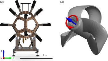
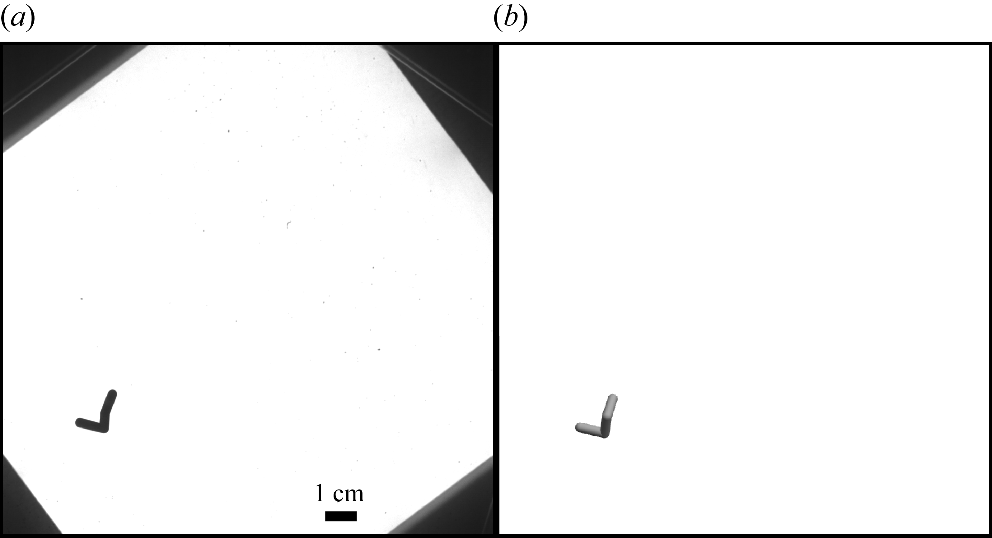
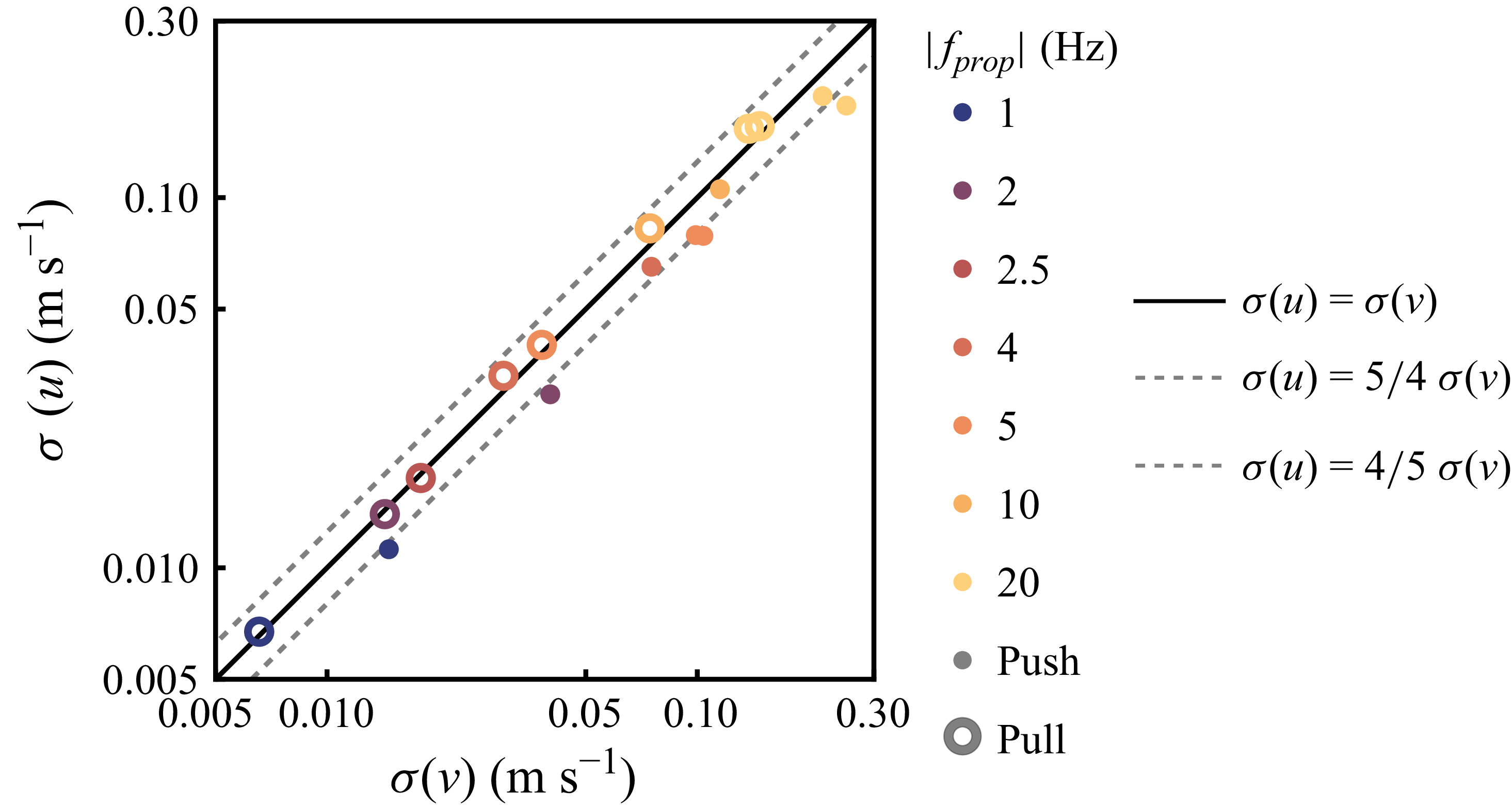
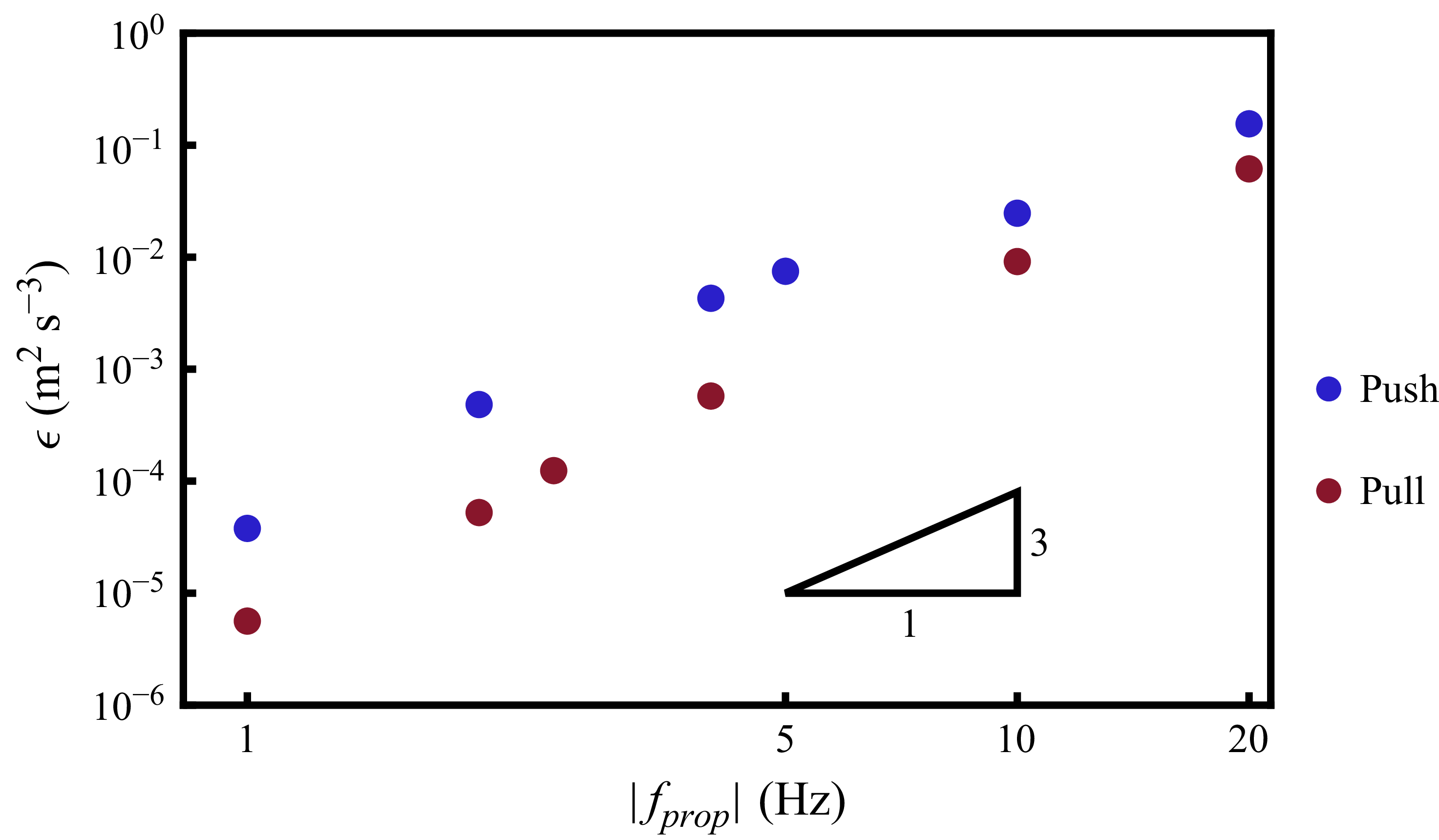
 ϵ
ϵ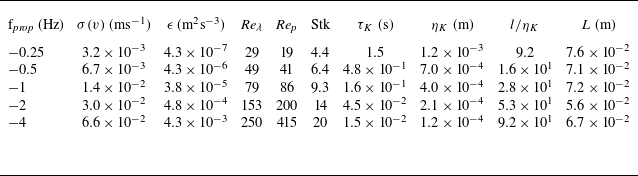

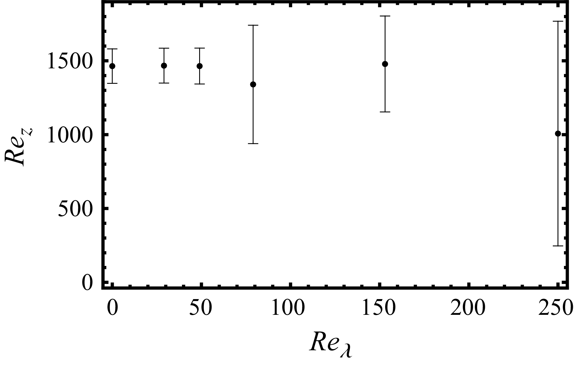
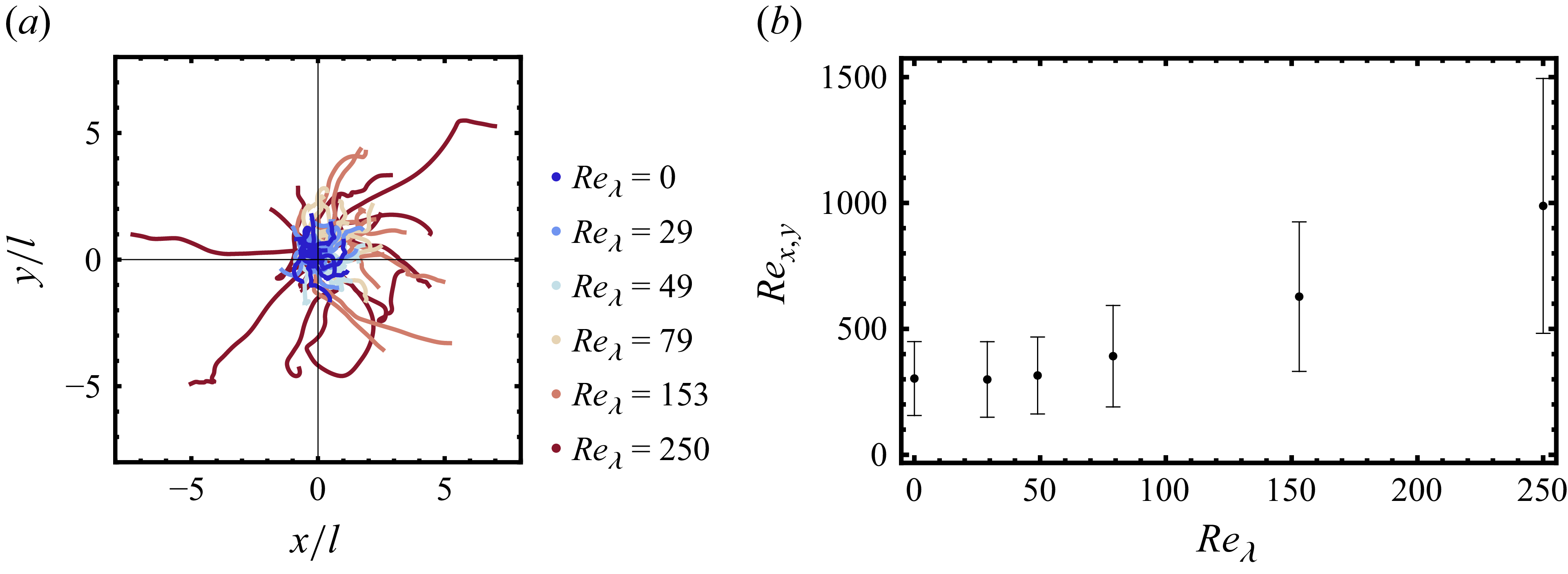


 Reλ=0
Reλ=0
 x
x y
y z
z α
α β
β γ
γ x
x y
y z
z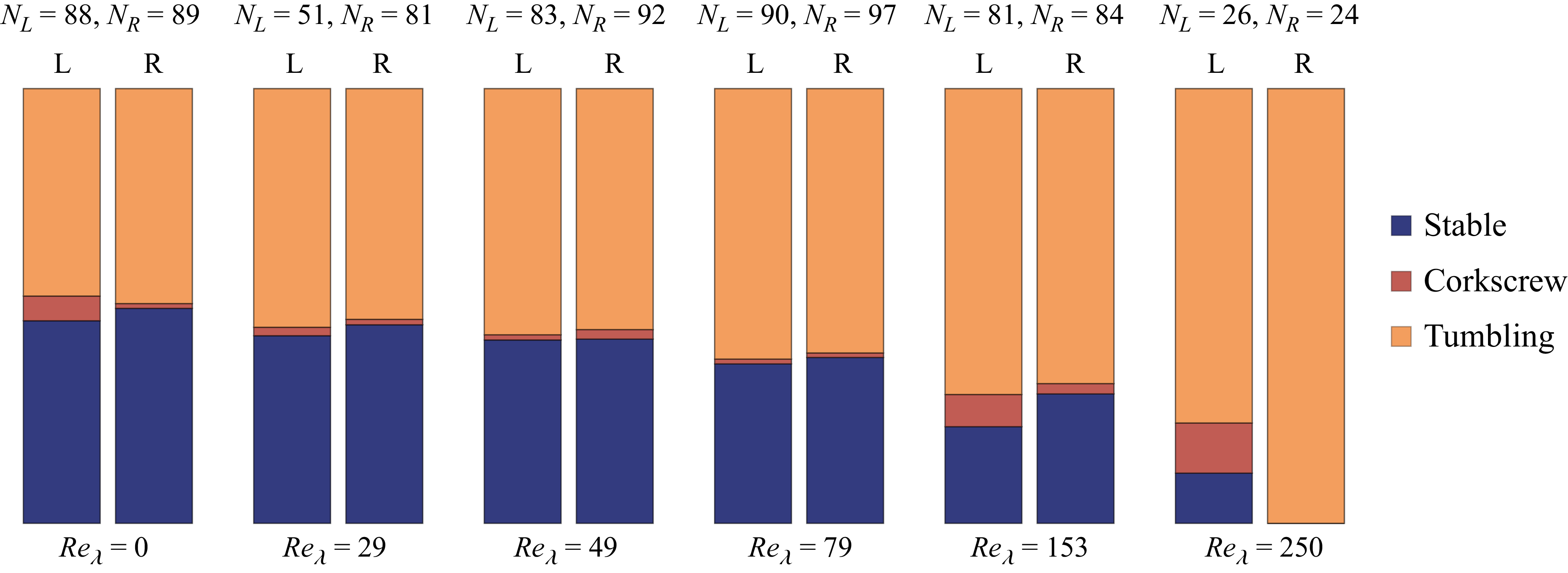

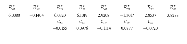
 r/d=0.1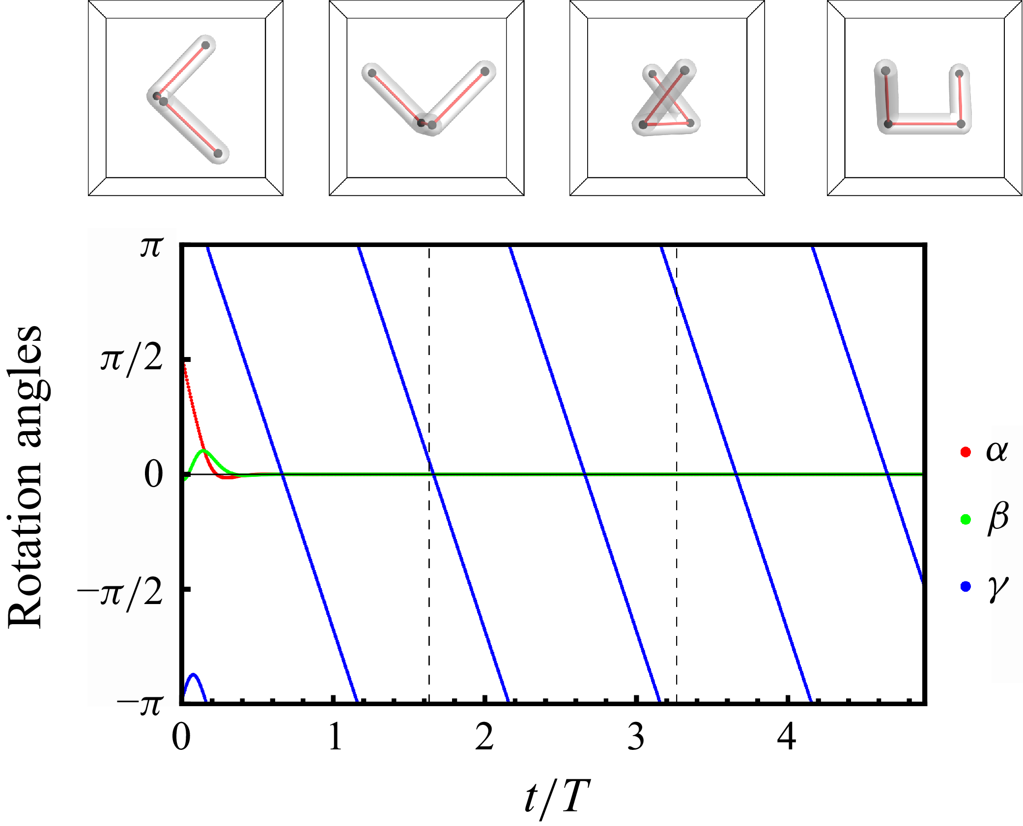


 f
f

 50%
50%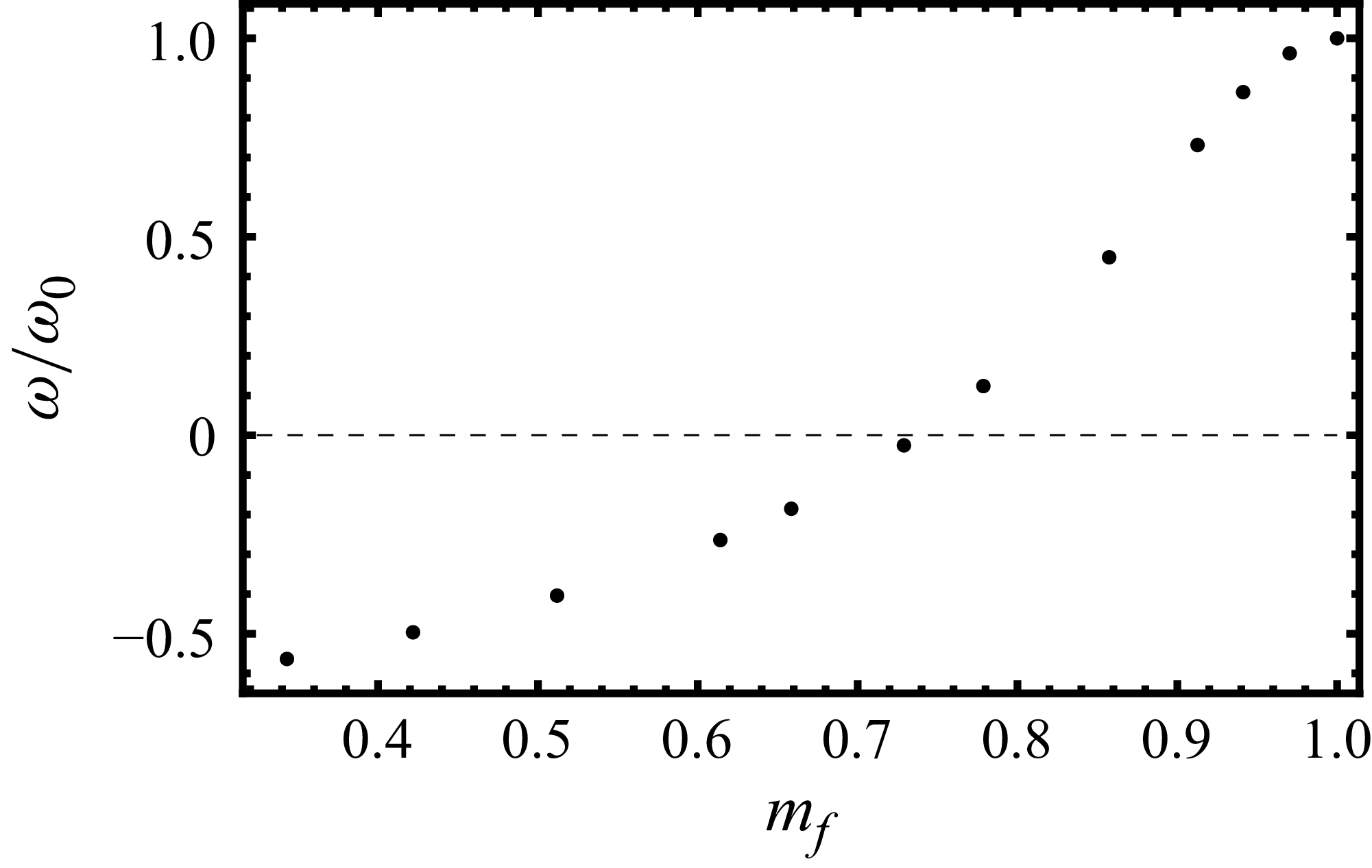
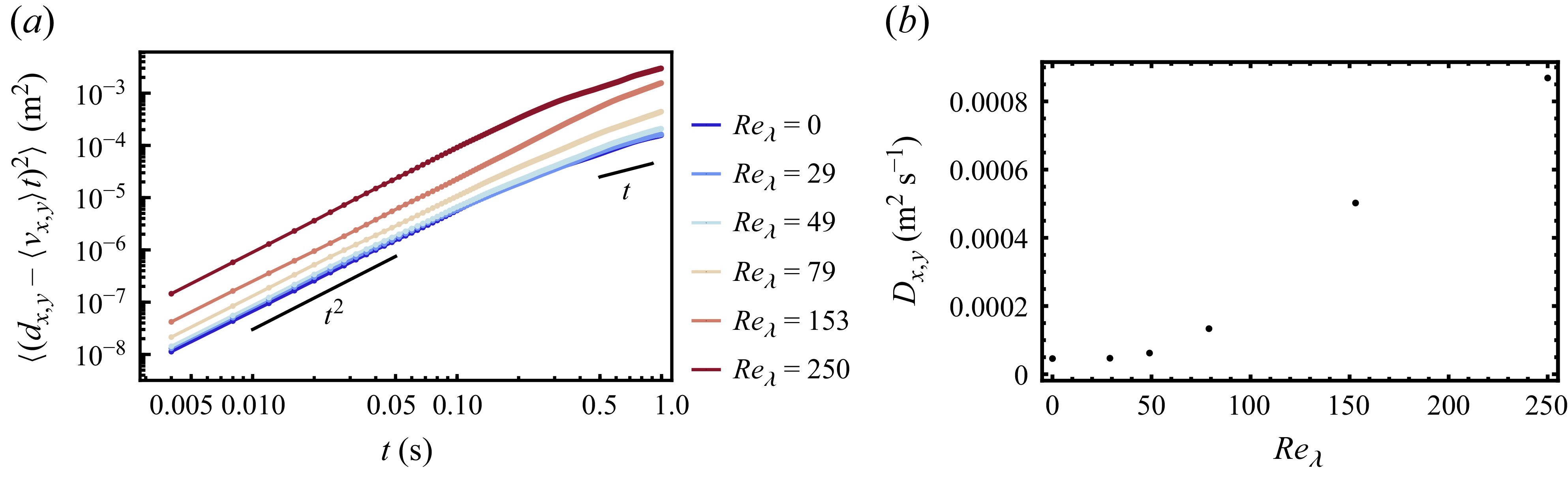
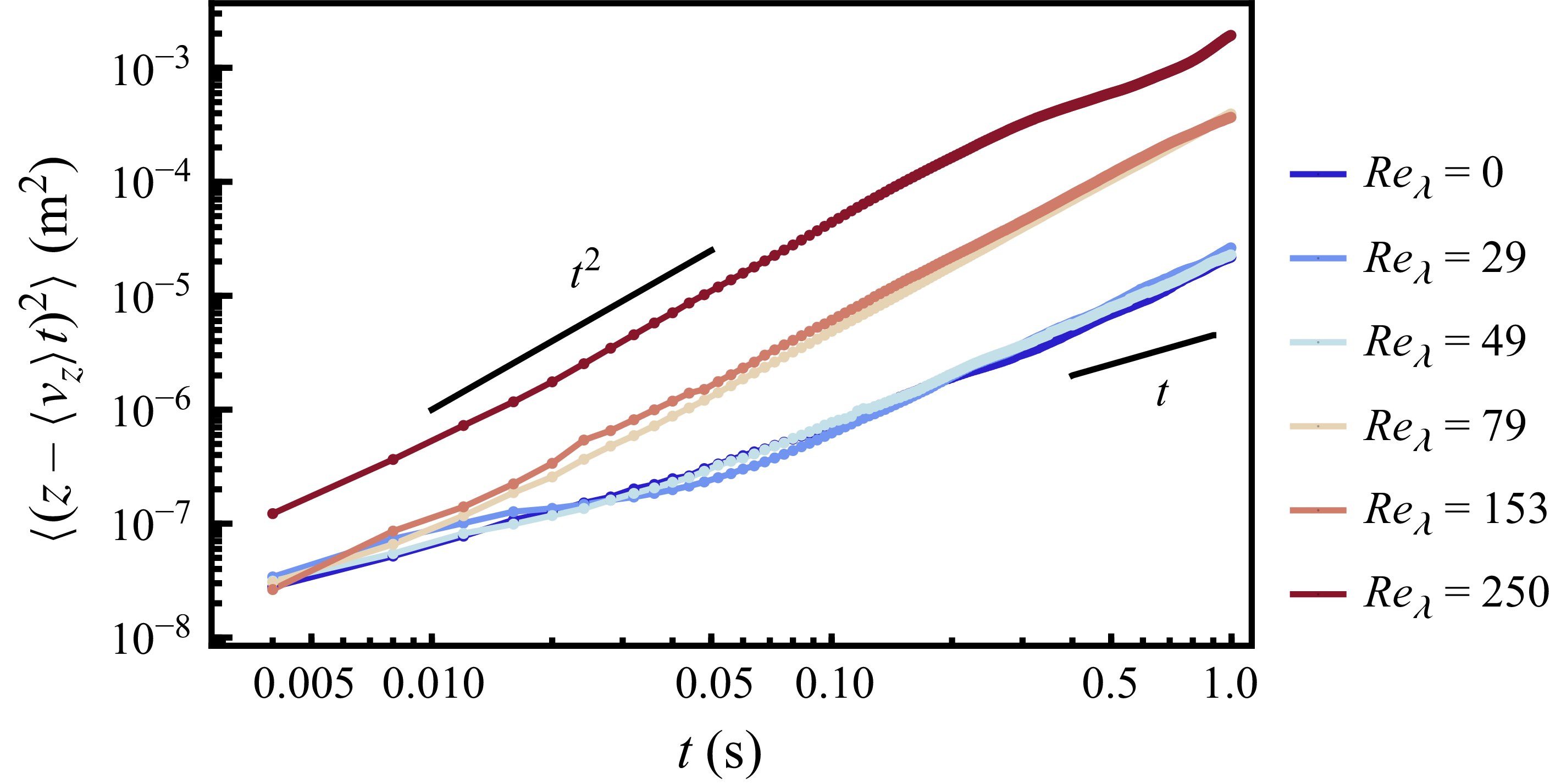
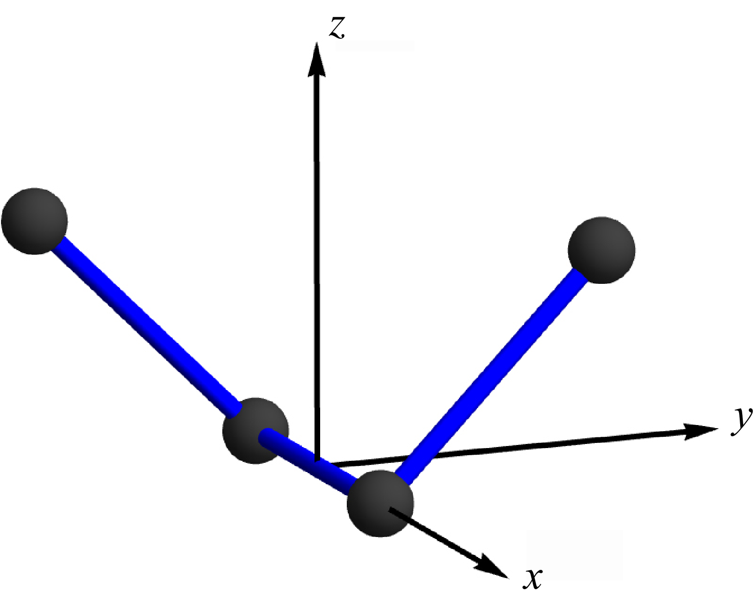
 r/d=0.1


 Open access

