


1. Introduction
Open traps are devices for magnetic plasma confinement where magnetic field lines intersect both the plasma surface and the end plates. This is a drawback, since parallel losses can be severe, but also an opportunity, since it opens a way to influence plasma motion by biasing external electrodes. Special complex measures are needed to stabilise plasma in axisymmetric open traps to flute type modes due to unfavourable average curvature (Ryutov et al. Reference Ryutov, Berk, Cohen, Molvik and Simonen2011). However, flute modes can also arise due to other sources of plasma polarisation besides the pressure gradient in a field with curvature. For instance, inflection points on the velocity profile are pivots for the Kelvin–Helmholtz (KH) instability (Helmholtz 1868); radially decreasing density causes centrifugal drive, or Rayleigh–Taylor (RT) instability of rotating plasma (Ariel & Bhatia Reference Ariel and Bhatia1970); inhomogeneity in electron temperature can also drive flute-like modes of the electron-temperature-gradient instability (Berk, Ryutov & Tsidulko Reference Berk, Ryutov and Tsidulko1990).
Flute modes cause turbulent eddies that effectively transport particles and heat from the hot core across flux surfaces out to the cooler plasma edge, degrading the plasma confinement. Turbulent transport determines the attainable pressure and fusion power in magnetic confinement devices and dominates collisional transport in the gradient regions. The flute-mode approximation imposes zero parallel electric field on possible perturbations. This assumption breaks for drift and ballooning modes, as well as many other types of perturbations that can cause turbulent transport while having their own stability conditions. In this paper we will consider the flute-type perturbations only, since they correspond to large-scale convection in gas-dynamic traps.
The gas-dynamic traps aim at confining dense plasma in mirrors with high mirror ratio. The namesake Gas-Dynamic Trap (GDT) (Ivanov & Prikhodko Reference Ivanov and Prikhodko2017) was designed and constructed at the Budker Institute of Nuclear Physics. Among all invented approaches to suppress flute transversal losses in mirror traps, GDT utilised several (Ryutov et al. Reference Ryutov, Berk, Cohen, Molvik and Simonen2011). The main stabilising method in GDT was satisfying Rosenbluth–Longmire criterion (Rosenbluth & Longmire Reference Rosenbluth and Longmire1957)
 \begin{equation} \int \text{d}l\dfrac {\pi _{\parallel }+\pi _{\perp }}{r\left (l\right )B^{2}}\varkappa \gt 0. \end{equation}
The integral in (1.1) is taken along the magnetic field line at radius $r(l)$
, where
$r(l)$
, where $\pi _{\parallel ,\perp }$
are momentum flux tensor components and
$\pi _{\parallel ,\perp }$
are momentum flux tensor components and $\varkappa$
is the magnetic field curvature. Criterion (1.1) is sufficient for stability and contains two experimentally adjustable quantities, the plasma pressure and the magnetic field curvature. Negative sign of
$\varkappa$
is the magnetic field curvature. Criterion (1.1) is sufficient for stability and contains two experimentally adjustable quantities, the plasma pressure and the magnetic field curvature. Negative sign of $\varkappa$
in the central region of axisymmetric mirror traps (1.1) can be compensated by pumping positive curvature regions, such as expanders, with hot and dense plasma. This was used in the initial GDT concept to satisfy the Rosenbluth–Longmire criterion (1.1). However, maintaining sufficiently dense plasma in expanders comes with the price of high axial losses, which is counterproductive to achieving high plasma parameters. The current mode of GDT operation relies on the plasma biasing via limiters and end plates instead.
$\varkappa$
in the central region of axisymmetric mirror traps (1.1) can be compensated by pumping positive curvature regions, such as expanders, with hot and dense plasma. This was used in the initial GDT concept to satisfy the Rosenbluth–Longmire criterion (1.1). However, maintaining sufficiently dense plasma in expanders comes with the price of high axial losses, which is counterproductive to achieving high plasma parameters. The current mode of GDT operation relies on the plasma biasing via limiters and end plates instead.
The magnetohydrodynamic (MHD) activity and transverse plasma confinement can be substantially affected by plasma rotation. The most efficient way to induce or affect such rotation in open traps is by biasing external electrodes (Volosov Reference Volosov2009). During the series of experiments by Bagryansky et al. (Reference Bagryansky, Lizunov, Zuev, Kolesnikov and Solomachin2003) on MHD stability of plasma in GDT the endwall plates were biased to 250–300 V in an attempt to compensate for the centrifugal effect of the ambipolar rotation. The observed increase in the confinement time, up to values predicted for pure axial losses in stable regimes, persisted even with zero curvature in expanders, i.e. with negative Rosenbluth–Longmire integral. Later, it was realised in Beklemishev & Chaschin (Reference Beklemishev and Chaschin2005) that the effect was caused by the differential rotation in plasma with a considerable finite-Larmor-radius (FLR) effect. The shear flow provides nonlinear saturation of convection inside a vortex, effectively separating the plasma core from the limiter, while the FLR effects of hot ions affect all modes except for the global mode with azimuthal wave number $m=1$
. The effect is significantly different from the usual suppression of convection by sheared flows. Namely, the unstable rigid
$m=1$
. The effect is significantly different from the usual suppression of convection by sheared flows. Namely, the unstable rigid $m=1$
mode corresponds to a shift of the plasma column together with the sheared flow, thus remaining unaffected by it. The nonlinear saturation is essentially due to the current dissipation at the biasing end plates, i.e. by the partial line-tying effect inherent to open traps. The corresponding confinement regime was called in Beklemishev et al. (Reference Beklemishev, Bagryansky, Chaschin and Soldatkina2010) the vortex confinement.
$m=1$
mode corresponds to a shift of the plasma column together with the sheared flow, thus remaining unaffected by it. The nonlinear saturation is essentially due to the current dissipation at the biasing end plates, i.e. by the partial line-tying effect inherent to open traps. The corresponding confinement regime was called in Beklemishev et al. (Reference Beklemishev, Bagryansky, Chaschin and Soldatkina2010) the vortex confinement.
Theoretical interpretation of the vortex confinement in GDT came out as a parametric nonlinear model of low $\beta$
plasma for electrostatic potential
$\beta$
plasma for electrostatic potential $\varphi$
and pressure
$\varphi$
and pressure $p$
$p$
 \begin{align} \dfrac {\partial \Delta \varphi }{\partial t}+\left \{ \varphi ,\Delta \varphi \right \} -U\boldsymbol{\nabla }\boldsymbol{\cdot }\left \{ \boldsymbol{\nabla }\varphi ,p\right \} & =H\left (\varphi -\varphi _{w}\right )+\varkappa \left \{ p,r^{2}\right \} +\nu _{\perp }\Delta ^{2}\varphi \nonumber\\&\quad -\nu _{\parallel }\Delta \varphi -U\Delta S_{p}, \end{align}
 \begin{align} \dfrac {\partial p}{\partial t}+\left \{ \varphi ,p\right \} &=\nu _{\perp }^{p}\Delta p-\nu _{\parallel }^{p}p+Q_{p}, \end{align}
where $\{ a,b\} \equiv a_{x}^{\prime }b_{y}^{\prime }-b_{x}^{\prime }a_{y}^{\prime }$
are the Poisson brackets, or Jacobian, in coordinates transverse to magnetic field lines. The dimensionless parameters are:
$\{ a,b\} \equiv a_{x}^{\prime }b_{y}^{\prime }-b_{x}^{\prime }a_{y}^{\prime }$
are the Poisson brackets, or Jacobian, in coordinates transverse to magnetic field lines. The dimensionless parameters are: $U$
describes the FLR effects,
$U$
describes the FLR effects, $H$
corresponds to the plasma–wall coupling,
$H$
corresponds to the plasma–wall coupling, $\varkappa$
is the mean field curvature,
$\varkappa$
is the mean field curvature, $\nu _{\perp }$
is the transverse viscosity,
$\nu _{\perp }$
is the transverse viscosity, $\nu _{\parallel }$
is the axial loss rate,
$\nu _{\parallel }$
is the axial loss rate, $S_{p}$
and
$S_{p}$
and $Q_{p}$
are the source terms,
$Q_{p}$
are the source terms, $\varphi _{w}(r)$
corresponds to the endwall-biasing potential.
$\varphi _{w}(r)$
corresponds to the endwall-biasing potential.
The line-tying effect, described by the parameter $H$
, is typically large in gas-dynamic traps (
$H$
, is typically large in gas-dynamic traps ( $H\gtrsim 10$
), while being lower (
$H\gtrsim 10$
), while being lower ( $H\lesssim 1$
) in tandem mirrors with suppressed axial losses. It is responsible for relaxation of the flux tube potential to the corresponding ambipolar potential due to axial currents to the end electrodes through Debye sheaths. The effect of Debye sheaths on currents is similar to thermocouple contacts, i.e. they introduce surface dissipation. Since the distribution of the potential is related to the transverse plasma motion, this effect is fundamental for the description of the plasma dynamics in open traps. At low electron temperatures the sheath potentials are negligible and the line tying is strong enough to suppress all flute modes. The line tying by itself is sufficient to slow down the low-
$H\lesssim 1$
) in tandem mirrors with suppressed axial losses. It is responsible for relaxation of the flux tube potential to the corresponding ambipolar potential due to axial currents to the end electrodes through Debye sheaths. The effect of Debye sheaths on currents is similar to thermocouple contacts, i.e. they introduce surface dissipation. Since the distribution of the potential is related to the transverse plasma motion, this effect is fundamental for the description of the plasma dynamics in open traps. At low electron temperatures the sheath potentials are negligible and the line tying is strong enough to suppress all flute modes. The line tying by itself is sufficient to slow down the low- $m$
modes in GDT and its planned successor Gas-Dynamic Multiple-Mirror Trap (GDMT) (Beklemishev et al. Reference Beklemishev2013; Skovorodin et al. Reference Skovorodin2023), but in combination with plasma biasing it serves as a foundation of the vortex confinement method.
$m$
modes in GDT and its planned successor Gas-Dynamic Multiple-Mirror Trap (GDMT) (Beklemishev et al. Reference Beklemishev2013; Skovorodin et al. Reference Skovorodin2023), but in combination with plasma biasing it serves as a foundation of the vortex confinement method.
The biasing scheme is essential to the vortex confinement. The scheme refers to relative spatial positions of the facility elements, e.g. limiters and endwall radii, to which potential is applied or grounded. The GDT experiments featured a positive potential of ${\sim}300$
V on the outer endwall plate and the limiter relative to the grounded vacuum chamber. The plasma confinement time measured by Thomson scattering (Bagryansky et al. Reference Bagryansky, Lizunov, Zuev, Kolesnikov and Solomachin2003) corresponded to purely gas-dynamic losses, meaning the absence of small-scale instability. This biasing often resulted in a discharge to the adjacent endwall plate. Reducing the potential resolved the issue; however, instability developed. To avoid complex and costly redesign, a positive potential was applied only to the limiter. With limiter-only biasing the energy confinement time decreased by 10 % compared with the purely gas-dynamic time using the same applied potential. The decrease is also associated with instability. For a GDT plasma with experiment duration of
${\sim}300$
V on the outer endwall plate and the limiter relative to the grounded vacuum chamber. The plasma confinement time measured by Thomson scattering (Bagryansky et al. Reference Bagryansky, Lizunov, Zuev, Kolesnikov and Solomachin2003) corresponded to purely gas-dynamic losses, meaning the absence of small-scale instability. This biasing often resulted in a discharge to the adjacent endwall plate. Reducing the potential resolved the issue; however, instability developed. To avoid complex and costly redesign, a positive potential was applied only to the limiter. With limiter-only biasing the energy confinement time decreased by 10 % compared with the purely gas-dynamic time using the same applied potential. The decrease is also associated with instability. For a GDT plasma with experiment duration of ${\sim}\,5$
ms these changes are not critical, while in longer lasting experiments instability can lead to significant energy losses. This experimental fact motivated a study of biasing schemes impact on vortex confinement.
${\sim}\,5$
ms these changes are not critical, while in longer lasting experiments instability can lead to significant energy losses. This experimental fact motivated a study of biasing schemes impact on vortex confinement.
The model (1.2, 1.3) was initially developed to explain the improved confinement in GDT experiments. For simplicity, it included only the curvature drive effects for the flute modes, using the paraxial approximation with low $\beta$
, uniform density and electron-temperature profiles, thus neglecting possible centrifugal and electron-temperature drives. In numerical simulations the model showed qualitative consistency with the GDT experiments with biasing potentials (Prikhodko et al. Reference Prikhodko, Bagryansky, Beklemishev, Kolesnikov, Kotelnikov, Maximov, Pushkareva, Soldatkina, Tsidulko and Zaytsev2011). Its main conclusion is that it is possible to operate the GDT-like traps with low convective losses while having nonlinearly saturated rotating
$\beta$
, uniform density and electron-temperature profiles, thus neglecting possible centrifugal and electron-temperature drives. In numerical simulations the model showed qualitative consistency with the GDT experiments with biasing potentials (Prikhodko et al. Reference Prikhodko, Bagryansky, Beklemishev, Kolesnikov, Kotelnikov, Maximov, Pushkareva, Soldatkina, Tsidulko and Zaytsev2011). Its main conclusion is that it is possible to operate the GDT-like traps with low convective losses while having nonlinearly saturated rotating $m=1$
or
$m=1$
or $m=2$
modes. That is provided certain conditions on the biasing potential and the axial loss rates are satisfied. However, limitations of the model can invalidate this conclusion in application to realistic experiments with non-uniform density and electron-temperature profiles. Understanding the role of the electron-temperature gradient and the related instability (Berk et al. Reference Berk, Ryutov and Tsidulko1990) is especially important in open traps, since they are coupled to the line-tying effect and the ambipolar potential. To distinguish this flute-mode electron-temperature-gradient instability in open traps from its drift-wave counterpart (Rudakov & Sagdeev Reference Rudakov and Sagdeev1961) we will denote it fETG in what follows. Furthermore, it would be prudent to include in simulations of GDT experiments (i) the motion and continuity equations for injected collisionless hot ions; (ii) the energy balance equations, including energy exchange among electrons, warm and hot ions; (iii) model source terms for neutral beam injectors and electron cyclotron resonance, etc.
$m=2$
modes. That is provided certain conditions on the biasing potential and the axial loss rates are satisfied. However, limitations of the model can invalidate this conclusion in application to realistic experiments with non-uniform density and electron-temperature profiles. Understanding the role of the electron-temperature gradient and the related instability (Berk et al. Reference Berk, Ryutov and Tsidulko1990) is especially important in open traps, since they are coupled to the line-tying effect and the ambipolar potential. To distinguish this flute-mode electron-temperature-gradient instability in open traps from its drift-wave counterpart (Rudakov & Sagdeev Reference Rudakov and Sagdeev1961) we will denote it fETG in what follows. Furthermore, it would be prudent to include in simulations of GDT experiments (i) the motion and continuity equations for injected collisionless hot ions; (ii) the energy balance equations, including energy exchange among electrons, warm and hot ions; (iii) model source terms for neutral beam injectors and electron cyclotron resonance, etc.
Another point of concern is the applicability of the electrostatic flute-mode approximation that essentially allowed two-dimensional reduction of the problem. This approximation is expected to be relevant at low relative plasma pressures $\beta \ll 1$
, while the operational values of
$\beta \ll 1$
, while the operational values of $\beta$
in GDT (Bagryansky et al. Reference Bagryansky2011) are of the order of 0.5. The finite-
$\beta$
in GDT (Bagryansky et al. Reference Bagryansky2011) are of the order of 0.5. The finite- $\beta$
effects should be significant, although the related ballooning instability has a higher threshold. It was shown in Bushkova & Mirnov (Reference Bushkova and Mirnov1985) and Kotelnikov et al. (Reference Kotelnikov, Zeng, Prikhodko, Yakovlev, Zhang, Chen and Yu2022) that the GDT plasma should be free of ballooning modes up to
$\beta$
effects should be significant, although the related ballooning instability has a higher threshold. It was shown in Bushkova & Mirnov (Reference Bushkova and Mirnov1985) and Kotelnikov et al. (Reference Kotelnikov, Zeng, Prikhodko, Yakovlev, Zhang, Chen and Yu2022) that the GDT plasma should be free of ballooning modes up to $\beta _{crit}\lesssim 0.7-0.8$
. The ballooning threshold may be exceeded in the next-generation device GDMT (Beklemishev et al. Reference Beklemishev2013), in which the new diamagnetic confinement regime (Beklemishev Reference Beklemishev2016) with
$\beta _{crit}\lesssim 0.7-0.8$
. The ballooning threshold may be exceeded in the next-generation device GDMT (Beklemishev et al. Reference Beklemishev2013), in which the new diamagnetic confinement regime (Beklemishev Reference Beklemishev2016) with $\beta \rightarrow 1$
will be tested. According to Kotelnikov et al. (Reference Kotelnikov, Zeng, Prikhodko, Yakovlev, Zhang, Chen and Yu2022), conductive walls around the plasma column can be effective in stabilising the ballooning modes in GDMT for
$\beta \rightarrow 1$
will be tested. According to Kotelnikov et al. (Reference Kotelnikov, Zeng, Prikhodko, Yakovlev, Zhang, Chen and Yu2022), conductive walls around the plasma column can be effective in stabilising the ballooning modes in GDMT for $\beta \gt 0.7$
. However, reaching this regime requires using the vortex confinement in the early stages of discharge (Skovorodin et al. Reference Skovorodin2023), as it is beyond the applicability of the original model. For this reason, electromagnetic generalisation of the vortex confinement model is in progress.
$\beta \gt 0.7$
. However, reaching this regime requires using the vortex confinement in the early stages of discharge (Skovorodin et al. Reference Skovorodin2023), as it is beyond the applicability of the original model. For this reason, electromagnetic generalisation of the vortex confinement model is in progress.
Motivation of the present paper is in adjusting the vortex confinement model to incorporate the density and electron-temperature gradients. We focus on the effects that are primarily caused by them, namely, the turbulent transport caused by centrifugal and the electron-temperature-gradient instabilities in presence of partial line tying. The role of these effects in biasing scheme efficiency is also considered. In § 2 we derive the generalised equations within the original framework of low- $\beta$
collisional plasma. Linear theory and modelling early stages of the centrifugal RT mode with FLR effects and of the fETG mode in the presence of partial line tying are gathered in § 3. Section 4 contains simulation-based estimates of the turbulent radial transport in the vortex confinement regime and comparison between different biasing schemes in original and extended models.
$\beta$
collisional plasma. Linear theory and modelling early stages of the centrifugal RT mode with FLR effects and of the fETG mode in the presence of partial line tying are gathered in § 3. Section 4 contains simulation-based estimates of the turbulent radial transport in the vortex confinement regime and comparison between different biasing schemes in original and extended models.
2. Extended equations
Before discussing generalisations, we briefly review the original vortex confinement model. The model is electrostatic, meaning that the magnetic field ${B}$
is unperturbed and paraxial, so that
${B}$
is unperturbed and paraxial, so that $\boldsymbol{B}=B_{v}\boldsymbol{b}\approx B_{v}\boldsymbol{e}_{z}$
. The equation for the dynamic vorticity (1.2) follows from the quasi-neutrality condition integrated over a field line
$\boldsymbol{B}=B_{v}\boldsymbol{b}\approx B_{v}\boldsymbol{e}_{z}$
. The equation for the dynamic vorticity (1.2) follows from the quasi-neutrality condition integrated over a field line
 \begin{equation} \int \dfrac {\text{d}\boldsymbol{l}}{B}\boldsymbol{\nabla }\boldsymbol{\cdot }\left (\boldsymbol{j}_{\perp }+\boldsymbol{j}_{\parallel }\right )=0, \end{equation}
where the transversal current density $\boldsymbol{j}_{\perp }$
is found from the equation of motion, while the transverse flow velocity is described via the scalar potential as
$\boldsymbol{j}_{\perp }$
is found from the equation of motion, while the transverse flow velocity is described via the scalar potential as
 \begin{equation} \boldsymbol{\upsilon }_{\perp }=\dfrac {c}{B_{v}}\boldsymbol{b}\times \boldsymbol{\nabla }\varphi . \end{equation}
The divergence of the transverse current translates into the time derivative of vorticity $\sim \Delta \varphi$
as well as all other terms related to transverse plasma motion in (1.2) under the assumption of a uniform distribution of the mass density.
$\sim \Delta \varphi$
as well as all other terms related to transverse plasma motion in (1.2) under the assumption of a uniform distribution of the mass density.
Meanwhile, the divergence of axial currents integrated between end plates (equation (1) in Beklemishev et al. Reference Beklemishev, Bagryansky, Chaschin and Soldatkina2010) yields
 \begin{equation} \int \dfrac {\text{d}l}{B}\boldsymbol{\nabla }\boldsymbol{\cdot }\boldsymbol{j}_{\parallel }\approx \left .\dfrac {j_{\parallel }}{B_{v}}\right |_{wall}\simeq j_{i}\dfrac {2e}{BT_{e}\left (r\right )}\left (\varphi -\varphi _{eq}\left (r\right )\right )\!, \end{equation}
where the equilibrium potential is a sum of ambipolar $\varLambda T_{e}/e$
and wall-biasing
$\varLambda T_{e}/e$
and wall-biasing $\varphi _{w}$
contributions:
$\varphi _{w}$
contributions: $ \varphi _{eq}(r)=\varLambda T_{e}(r)/e+\varphi _{w}(r)$
. The electron temperature
$ \varphi _{eq}(r)=\varLambda T_{e}(r)/e+\varphi _{w}(r)$
. The electron temperature $T_{e}$
appears in (2.3) since the end-plate current flows over the Debye sheath, while the approximation is valid for
$T_{e}$
appears in (2.3) since the end-plate current flows over the Debye sheath, while the approximation is valid for $e(\varphi -\varphi _{eq}(r))/T_{e}\ll 1$
. Electron temperature is uniform in the original model and enters as an external parameter. Integration along the equilibrium field lines is straightforward as long as the plasma motion is considered low-
$e(\varphi -\varphi _{eq}(r))/T_{e}\ll 1$
. Electron temperature is uniform in the original model and enters as an external parameter. Integration along the equilibrium field lines is straightforward as long as the plasma motion is considered low- $\beta$
electrostatic. The model essentially assumes
$\beta$
electrostatic. The model essentially assumes $\partial \varphi /\partial l=0$
up to Debye sheaths at the limiter or the endwall plates, where the external biasing potentials
$\partial \varphi /\partial l=0$
up to Debye sheaths at the limiter or the endwall plates, where the external biasing potentials $\varphi _{w}$
are applied.
$\varphi _{w}$
are applied.
In the extended model we aim to relax the stringent assumptions $n,T_{e}=const$
while preserving the essential framework and simplicity of the original. Redistribution of the mass density changes the divergence of the polarisation current
$n,T_{e}=const$
while preserving the essential framework and simplicity of the original. Redistribution of the mass density changes the divergence of the polarisation current $\boldsymbol{j}_{p}=c[\boldsymbol{b}\times nd_{t} \boldsymbol{\upsilon }_{\perp }]/B$
that accounts for the inertial terms in (1.2). Integrated along a field line it becomes
$\boldsymbol{j}_{p}=c[\boldsymbol{b}\times nd_{t} \boldsymbol{\upsilon }_{\perp }]/B$
that accounts for the inertial terms in (1.2). Integrated along a field line it becomes
 \begin{equation} \int \dfrac {\text{d}l}{B}\boldsymbol{\nabla }\boldsymbol{\cdot }\boldsymbol{j}_{p}\approx -\dfrac {c}{B_{v}}\dfrac {\text{d}\varpi }{\text{d}t}+\left (\dfrac {c}{B_{v}}\right )^{3}\left \{ n,\dfrac {\left (\boldsymbol{\nabla }\varphi \right )^{2}}{2}\right\}\!, \end{equation}
where the dynamic part of generalised vorticity $\varpi$
is defined by
$\varpi$
is defined by
 \begin{equation} \varpi \equiv \boldsymbol{e}_{z}\boldsymbol{\cdot }\boldsymbol{\nabla }\times \left (n\boldsymbol{\upsilon }_{\perp }\right )=\dfrac {c}{B_{v}}\boldsymbol{\nabla }\boldsymbol{\cdot }\left (n\boldsymbol{\nabla }\varphi \right)\!. \end{equation}
While deriving (2.4) we used the continuity equation for plasma density $n$
with incompressible transverse convection, the source
$n$
with incompressible transverse convection, the source $S_{n}$
, transverse diffusion and axial losses as follows:
$S_{n}$
, transverse diffusion and axial losses as follows:
 \begin{equation} \dfrac {\partial n}{\partial t}+\left \{ \varphi ,n\right \} =\nu _{\perp }^{n}\Delta n-\nu _{\parallel }^{n}n+S_{n}. \end{equation}
It closely follows the reasoning behind (1.2) of the original model. In order to keep the model two potential, all three distributed scalars in what follows are unified $T_{e}\sim p_{i}\sim n$
. This can be justified if the ion–electron energy exchange is fast enough and the heat conductivity makes the model equivalent to the isothermic case, although we do not assume it explicitly. These assumptions allow us to ignore some other terms emerging in (2.4) in a more general setting.
$T_{e}\sim p_{i}\sim n$
. This can be justified if the ion–electron energy exchange is fast enough and the heat conductivity makes the model equivalent to the isothermic case, although we do not assume it explicitly. These assumptions allow us to ignore some other terms emerging in (2.4) in a more general setting.
Plasma rotation caused by the density inhomogeneity leads to emergence of the second term of (2.4) proportional to ${\sim\!(\boldsymbol{\nabla }\varphi)}^{2}$
, responsible for description of the centrifugal effect. Since the evolution of the electron temperature in our two-potential model follows the evolution of density, it is straightforward to incorporate (2.3) in (2.1) including the effects of non-uniform temperature. With additional terms we get the following equation for dynamic vorticity:
${\sim\!(\boldsymbol{\nabla }\varphi)}^{2}$
, responsible for description of the centrifugal effect. Since the evolution of the electron temperature in our two-potential model follows the evolution of density, it is straightforward to incorporate (2.3) in (2.1) including the effects of non-uniform temperature. With additional terms we get the following equation for dynamic vorticity:
 \begin{eqnarray} &&\dfrac {\partial \varpi }{\partial t}+\left \{ \varphi ,\varpi \right \} -\left \{ n,\dfrac {\left (\boldsymbol{\nabla }\varphi \right )^{2}}{2}\right \} -U\boldsymbol{\nabla }\boldsymbol{\cdot }\left \{ \boldsymbol{\nabla }\varphi ,n\right \} \nonumber \\ &&\quad =\dfrac {H}{n}\left (\varphi -\varLambda n-\varphi _{w}\right )+\varkappa \left \{ n,r^{2}\right \} +\nu _{\perp }\Delta \varpi -\nu _{\parallel }\varpi -U\Delta S_{n}. \end{eqnarray}
Equation (2.7) incorporates the effects of distributed density, electron temperature and plasma pressure using a single active scalar convection equation, so we will refer to it as a hybrid model.
3. Linear stages
We consider any of the instabilities in isolated form without other sources of polarisation. An instability develops from an axially symmetric initial state with small angular perturbations $\sim \text{exp}(im\theta -i\omega t)$
. The unperturbed initial potential matches the solid-body rotation
$\sim \text{exp}(im\theta -i\omega t)$
. The unperturbed initial potential matches the solid-body rotation $\partial _{r}\varphi _{0}=\varOmega r$
, where
$\partial _{r}\varphi _{0}=\varOmega r$
, where $\varOmega =const$
to avoid inflection points and eradicate the KH instability.
$\varOmega =const$
to avoid inflection points and eradicate the KH instability.
The spectrum of initial perturbations is specified by the boundary conditions and determined by a second-order ordinary differential equation (ODE) on the perturbation of potential $\varphi$
, which generally does not have an analytical solution. We are not interested in the solution itself, but in the growth of a given initial perturbation. For this purpose, we construct a local approximation in a form convenient for modelling. The initial distribution for a scalar
$\varphi$
, which generally does not have an analytical solution. We are not interested in the solution itself, but in the growth of a given initial perturbation. For this purpose, we construct a local approximation in a form convenient for modelling. The initial distribution for a scalar $f$
is defined as a function of radius
$f$
is defined as a function of radius
 \begin{equation} f\left (r\right )=A\left (\tanh\left (\dfrac {r-r_{0}}{\delta }\right )+B\right )\!, \end{equation}
and schematically shown in figure 1. Coefficients $A$
and
$A$
and $B$
are defined in such a way that
$B$
are defined in such a way that $f$
is normalised to the maximum value on the axis
$f$
is normalised to the maximum value on the axis $f(0)=1$
and to the background value away from the axis
$f(0)=1$
and to the background value away from the axis $f(\infty )=f_{bgd}$
.
$f(\infty )=f_{bgd}$
.
Sketch for the distribution (3.1).

The scalar $f$
smoothly changes from the axial to the background value in the neighbourhood
$f$
smoothly changes from the axial to the background value in the neighbourhood $\delta$
around radius
$\delta$
around radius $r_{0}$
passing its inflection point
$r_{0}$
passing its inflection point $\partial _{r}f(r=r_{0})=0$
. The gradient scale of the distribution (3.1)
$\partial _{r}f(r=r_{0})=0$
. The gradient scale of the distribution (3.1)
 \begin{equation} a_{f}\left (r\right )=\left (\partial _{r}lnf\right )^{-1} \end{equation}
determines the instability increment. Gradient scale (3.2) of monotonically decreasing distribution (3.1) is always negative and has extrema $a_{0}=-\left |a_{f}\right |_{r=r_{0}}=\delta (1+B)$
that coincide with the differential width
$a_{0}=-\left |a_{f}\right |_{r=r_{0}}=\delta (1+B)$
that coincide with the differential width $\delta$
to the relative background. The initial perturbation localised near
$\delta$
to the relative background. The initial perturbation localised near $r_{0}$
is numerically determined by the width
$r_{0}$
is numerically determined by the width $\delta$
controlled in the computer simulations. The width does not exceed the localisation radius providing computational domain boundary
$\delta$
controlled in the computer simulations. The width does not exceed the localisation radius providing computational domain boundary
 \begin{equation} 0\lt \delta \leq r_{0}. \end{equation}
Behaviour of $\varphi$
inside the width is described by the local variable
$\varphi$
inside the width is described by the local variable $x$
based on the localisation radius
$x$
based on the localisation radius $r=r_{0}+x$
. The spectrum of localised modes
$r=r_{0}+x$
. The spectrum of localised modes $x\ll 2\pi r_{0}/m$
is then determined by a harmonic oscillator with damping
$x\ll 2\pi r_{0}/m$
is then determined by a harmonic oscillator with damping
 \begin{equation} \varphi _{\textit{xx}}^{\prime \prime }+2\unicode {x03B3}\varphi _{x}^{\prime }+\omega _{0}^{2}\varphi =0. \end{equation}
The prime symbol denotes derivative with respect to spatial coordinate. Transition to flat geometry is equivalent to $r\rightarrow \infty$
or
$r\rightarrow \infty$
or $(k_{r},k_{x})\rightarrow 0$
, so the (3.4) reduces to its zero mode
$(k_{r},k_{x})\rightarrow 0$
, so the (3.4) reduces to its zero mode
 \begin{equation} \omega _{0}^{2}=0. \end{equation}
The last equation relates the initial parameters of distributed profiles with frequency $\omega$
. In case the radial structure is important, it is necessary to solve the boundary value problem
$\omega$
. In case the radial structure is important, it is necessary to solve the boundary value problem $\varphi (x=\pm \Delta r)=0$
,
$\varphi (x=\pm \Delta r)=0$
, $\varphi _{x}^{\prime }(x=0)=0$
corresponding to the localised perturbations of size
$\varphi _{x}^{\prime }(x=0)=0$
corresponding to the localised perturbations of size $\Delta r$
.
$\Delta r$
.
3.1. On computer simulations
We focus on analytics and simulations in the linear stages mostly for validation of our computer model. The computer model is based on the explicit first order in time and second order in space approximation of equations on a rectangular grid. The Poisson brackets are evaluated using the second-order Arakawa (Reference Arakawa1966) method. The inhomogeneous Poisson equation, (2.5), is solved for potential $\varphi$
using preconditioned conjugate gradient algorithm 2 described in Fisicaro et al. (Reference Fisicaro, Genovese, Andreussi, Marzari and Goedecker2016).
$\varphi$
using preconditioned conjugate gradient algorithm 2 described in Fisicaro et al. (Reference Fisicaro, Genovese, Andreussi, Marzari and Goedecker2016).
The background continuum value provides numerical stability for temperature and density associated effects. Background density is only added to the definition of general vorticity, and background temperature to the denominator of the line-tying term; the rest of the equations remain unchanged with such substitution. More generally, there is a neutral gas in the limiter’s shade that interacts with plasma. Radial flows generated by these gas–plasma interactions are not considered. We keep the background low in our numerical implementation to balance stability and performance. The corresponding numerical value of the background does not exceed 10 % of the peak density and 1 % of the peak electron temperature.
The choice for $m=5$
initial stages of RT and fETG instabilities from figures 2 and 4 is for demonstration purpose only.
$m=5$
initial stages of RT and fETG instabilities from figures 2 and 4 is for demonstration purpose only.
3.2. Rayleigh–Taylor instability of rotating plasma
Centrifugal drive in plasma is a consequence of radially inhomogeneous rotation. It can be thought as a RT instability in effective anti-gravitation generated in a rotating reference frame. Interpretation of a centrifugally forced RT instability in liquid can be found in Scase & Hill (Reference Scase and Hill2018). We include FLR effects for the isolated instability configuration in the following system:
 \begin{align} \dfrac {\text{d}}{\text{d}t}\boldsymbol{\nabla }\boldsymbol{\cdot }\left (n\boldsymbol{\nabla }\varphi \right )&=\left \{ n,\dfrac {\left (\boldsymbol{\nabla }\varphi \right )^{2}}{2}\right \} +U\boldsymbol{\nabla }\boldsymbol{\cdot }\left \{ \boldsymbol{\nabla }\varphi ,n\right \}\! ,\\[-10pt]\nonumber \end{align}
 \begin{align} \dfrac {\text{d}}{\text{d}t}n&=0. \end{align}
The Lagrangian derivative operator for rigid rotation
 \begin{equation} d_{t}=-i\omega +\varOmega \partial _{\theta }-imr^{-1}\varphi \partial _{r} \end{equation}
provides relation between perturbations of density and potential $n=\varphi n_{0}^{\prime }/(\varOmega r\mathcal{R})$
from (3.7), where
$n=\varphi n_{0}^{\prime }/(\varOmega r\mathcal{R})$
from (3.7), where
 \begin{equation} \mathcal{R}={1-\omega}/{(m\varOmega)} , \end{equation}
is the normalised rotational frequency factor. Linearising the substantial derivative of vorticity, centrifugal and FLR terms results in an ODE in the form (3.4) for the perturbation of the potential
 \begin{equation} \varphi _{rr}^{\prime \prime }+\varphi _{r}^{\prime }\left [\dfrac {1}{r}+\dfrac {1}{a_{n}}+\widetilde {U}g_{n1}\right ]/\left [1+\widetilde {U}\right ]+\varphi \left [F_{n}-\dfrac {m^{2}}{r^{2}}+\widetilde {U}g_{n2}\right ]/\left [1+\widetilde {U}\right ]=0, \end{equation}
where $a_{n}(r)$
is a density gradient scale and coefficients are
$a_{n}(r)$
is a density gradient scale and coefficients are
 \begin{gather} \widetilde {U}\left (r\right )=\dfrac {U}{a_{n}r\mathcal{R}\varOmega },\,\,\,F_{n}\left (r\right )=\dfrac {1}{a_{n}r\mathcal{R}}\left (\dfrac {1}{\mathcal{R}}-2\right )\!,\nonumber \\[9pt] g_{n1}\left (r\right )=\dfrac {1-a_{n}^{\prime }}{a_{n}}-\dfrac {1}{r\mathcal{R}},\,\,\,g_{n2}\left (r\right )=\dfrac {1}{r^{2}\mathcal{R}}-\dfrac {1-a_{n}^{\prime }}{a_{n}r\mathcal{R}}-\dfrac {m^{2}}{r^{2}}. \end{gather}
Following the locality (3.5), the fundamental frequency $\omega _{0}$
for the potential perturbation vanishes, resulting in equation
$\omega _{0}$
for the potential perturbation vanishes, resulting in equation
 \begin{equation} \left [F_{n}\left (r_{0}\right )-\dfrac {m^{2}}{r_{0}^{2}}+\widetilde {U}\left (r_{0}\right )g_{n2}\left (r_{0}\right )\right ]/\left [1+\widetilde {U}\left (r_{0}\right )\right ]=0. \end{equation}
The local spectrum of isolated RT instability is fully defined by the function $F_{n}$
, while
$F_{n}$
, while $g_{n1,2}$
contribute only in the case of the FLR effect.
$g_{n1,2}$
contribute only in the case of the FLR effect.
3.3. Hydrodynamic rigid rotation
In the absence of FLR effects, the instability reduces to a pure hydrodynamic regime. Early stages of instability onset are illustrated in figure 2. Equation (3.12) becomes a dispersion relation
 \begin{equation} \left (\mathcal{R}-\alpha \right )^{2}=\alpha ^{2}-\alpha , \end{equation}
where $\alpha =m^{-2}r_{0}/\delta$
.
$\alpha =m^{-2}r_{0}/\delta$
.
The onset of $m=5$
hydrodynamic RT instability.
$m=5$
hydrodynamic RT instability.

One of the roots of (3.13) is unstable and has a maximum $\varGamma ^{\star }\equiv \mathcal{I}m(\mathcal{R}_{\alpha =\alpha ^{\star }})$
at
$\varGamma ^{\star }\equiv \mathcal{I}m(\mathcal{R}_{\alpha =\alpha ^{\star }})$
at
 \begin{equation} \alpha ^{\star }=\dfrac {1}{2},\,\,\varGamma ^{\star }=\varOmega \left (2\dfrac {\delta }{r_{0}}\right )^{-1/2}\equiv \dfrac {m\varOmega }{2}. \end{equation}
The $\varGamma ^{\star }$
curve passes through all the maxima for a fixed
$\varGamma ^{\star }$
curve passes through all the maxima for a fixed $m\in \mathbb{N}$
(figure 3, dashed black curve). There is no instability for
$m\in \mathbb{N}$
(figure 3, dashed black curve). There is no instability for $\delta /r_{0}\leq m^{-2}$
and the equality corresponds to the cutoff
$\delta /r_{0}\leq m^{-2}$
and the equality corresponds to the cutoff $\alpha _{cut}=1$
. As
$\alpha _{cut}=1$
. As $m\rightarrow \infty$
, an initial perturbation becomes increasingly localised and instability develops at smaller gradient scales down to the limit of an infinitely sharp boundary
$m\rightarrow \infty$
, an initial perturbation becomes increasingly localised and instability develops at smaller gradient scales down to the limit of an infinitely sharp boundary $\delta \rightarrow 0$
. The global maximum growth rate
$\delta \rightarrow 0$
. The global maximum growth rate $\varGamma _{max}$
is the maximum over all possible
$\varGamma _{max}$
is the maximum over all possible $m$
$m$
 \begin{equation} \alpha _{max}\rightarrow 0,\,\,\varGamma _{max}=\varOmega \left (\dfrac {\delta }{r_{0}}\right )^{-1/2}, \end{equation}
and always exceeds the maximum growth rate for a fixed azimuthal mode $\varGamma _{max}=\sqrt {2}\varGamma ^{\star }$
. The parameter
$\varGamma _{max}=\sqrt {2}\varGamma ^{\star }$
. The parameter $\varGamma _{max}$
is an enveloping curve above all
$\varGamma _{max}$
is an enveloping curve above all $\varGamma _{m\lt \infty }$
(figure 3, solid black curve). The global
$\varGamma _{m\lt \infty }$
(figure 3, solid black curve). The global $m=1$
mode is not excited even if the initial perturbation is “localised” in the width of entire plasma, since its cutoff is on the boundary of computational domain (3.3).
$m=1$
mode is not excited even if the initial perturbation is “localised” in the width of entire plasma, since its cutoff is on the boundary of computational domain (3.3).


3.4. Stabilisation by FLR
In case of FLR effects the dispersion (3.13) modifies into
 \begin{equation} \left (\mathcal{R}-\alpha _{\widehat {U}}\right )^{2}=\alpha _{\widehat {U}}^{2}-\alpha _{\widehat {U}}\dfrac {1+\widehat {U}}{1+ {m^{2}}/{2}\widehat {U}}, \end{equation}
where coefficients $\alpha _{\widehat {U}}=\alpha (1+m^{2}\widehat {U}/2)$
and
$\alpha _{\widehat {U}}=\alpha (1+m^{2}\widehat {U}/2)$
and $\widehat {U}=U/(\varOmega r_{0}^{2})$
. Its unstable solution has an additional resonant condition
$\widehat {U}=U/(\varOmega r_{0}^{2})$
. Its unstable solution has an additional resonant condition $\omega _{\widehat {U}}\neq m\varOmega (1-\widehat {U}r_{0}/\delta )$
following from the singularity in (3.12) and reaches its maximum at
$\omega _{\widehat {U}}\neq m\varOmega (1-\widehat {U}r_{0}/\delta )$
following from the singularity in (3.12) and reaches its maximum at
 \begin{equation} \alpha _{\widehat {U}}^{\star }=\dfrac {1}{2}\dfrac {1+\widehat {U}}{1+ {m^{2}}/{2}\widehat {U}},\,\,\varGamma _{\widehat {U}}^{\star }=\dfrac {m\varOmega }{2}\dfrac {2\left (1+\widehat {U}\right )}{2+m^{2}\widehat {U}}. \end{equation}
The FLR motion affects modes with $m\gtrsim 2$
and increases with
$m\gtrsim 2$
and increases with $m$
. Figure 3(b) illustrates the FLR changes to the
$m$
. Figure 3(b) illustrates the FLR changes to the $m=7$
RT mode, showing its complete stabilisation within the computational domain at
$m=7$
RT mode, showing its complete stabilisation within the computational domain at $U\approx 0.283$
. The global maximum growth rate
$U\approx 0.283$
. The global maximum growth rate $\varGamma _{max}$
is absent as with
$\varGamma _{max}$
is absent as with $m\rightarrow \infty$
the stabilising effect of FLR turns out to be infinite. Asymptotic behaviour of
$m\rightarrow \infty$
the stabilising effect of FLR turns out to be infinite. Asymptotic behaviour of $\varGamma _{max}$
follows from root expansion in (3.16) providing a triggering condition for the instability
$\varGamma _{max}$
follows from root expansion in (3.16) providing a triggering condition for the instability
 \begin{equation} U\lt 2\varOmega r_{0}^{2}m^{-1}\left (\dfrac {\delta }{r_{0}}\right )^{1/2}+\mathcal{O}\left (m^{-2}\right)\!. \end{equation}
Estimate (3.18) shows stabilisation of localised modes in rigid rotation for lower $m\sim 1$
with GDT associated parameters
$m\sim 1$
with GDT associated parameters $U_{GDT}\approx 5$
and is consistent with numerical modelling. Similarities between pure RT and FLR-stabilised RT increments lead to the interpretation of FLR effect on RT instability given in Appendix A.
$U_{GDT}\approx 5$
and is consistent with numerical modelling. Similarities between pure RT and FLR-stabilised RT increments lead to the interpretation of FLR effect on RT instability given in Appendix A.
3.5. The flute electron-temperature-gradient instability
The fETG instability develops in open traps plasma with axial currents as a coupled effect of electron-temperature gradient and conducting end plates. The GDT axial currents are utilised for vortex transport barrier generation becoming the source for this instability. The fETG drive has been studied in different geometries and regimes. Berk et al. (Reference Berk, Ryutov and Tsidulko1990) considered the isolated fETG in a slab geometry. In later work, Berk, Ryutov & Tsidulko (Reference Berk, Ryutov and Tsidulko1991) derived a dispersion equation in flux coordinates including centrifugal drift and showed regimes with FLR stabilisation. We consider isolated fETG instability with axial loss. Energy dissipation is added to the Lagrangian derivative operator $d_{t}^{(\gamma )}\equiv d_{t}+\gamma H$
, where
$d_{t}^{(\gamma )}\equiv d_{t}+\gamma H$
, where $\gamma$
is a factor to electron-temperature axial losses
$\gamma$
is a factor to electron-temperature axial losses
 \begin{equation} \nu _{\parallel }^{\left (e\right )}=H\left (\dfrac {\rho _{i}}{r_{0}}\right )^{2}\dfrac {\tau _{\parallel i}}{\tau _{\parallel e}}=\gamma H. \end{equation}
This multiple $\gamma \approx 1$
for GDT parameters causes electrons to lose all their energy on a time scale of
$\gamma \approx 1$
for GDT parameters causes electrons to lose all their energy on a time scale of $\sim 0.3\,\text{ms}$
without external sources of energy. In the linear stages theory and simulations, we consider electron axial losses 10 times those of the warm plasma
$\sim 0.3\,\text{ms}$
without external sources of energy. In the linear stages theory and simulations, we consider electron axial losses 10 times those of the warm plasma $\nu _{\parallel }^{(e)}=10\nu _{\parallel GDT}\sim 0.2$
. The fETG-isolated model with substantial derivative operator containing energy dissipation is
$\nu _{\parallel }^{(e)}=10\nu _{\parallel GDT}\sim 0.2$
. The fETG-isolated model with substantial derivative operator containing energy dissipation is
 \begin{align} \left (\dfrac {\text{d}}{\text{d}t}\right )^{\left (\gamma \right )}T_{e}\boldsymbol{\nabla} ^{2}\varphi &=H\left (\varphi -\varLambda T_{e}\right )\!,\\[-10pt]\nonumber \end{align}
 \begin{align} \left (\dfrac {\text{d}}{\text{d}t}\right )^{\left (\gamma \right )}T_{e}&=0, \end{align}
where we re-assigned the hybrid scalar $n$
to be electron temperature
$n$
to be electron temperature $T_e$
. The following steps are the same as for isolated RT mode. The ODE for the perturbation of potential is as follows:
$T_e$
. The following steps are the same as for isolated RT mode. The ODE for the perturbation of potential is as follows:
 \begin{equation} \varphi _{rr}^{\prime \prime }+\varphi _{r}^{\prime }\dfrac {1}{r}+\varphi \left [F_{T_{e}}-\dfrac {m^{2}}{r^{2}}\right ]=0. \end{equation}
The spectrum is defined by the function
 \begin{equation} F_{T_{e}}\left (r\right )=-\dfrac {iH\varLambda m}{a_{T_{e}}r\left (m\varOmega \mathcal{R}_{\gamma }\right )^{2}}+\dfrac {iH}{T_{e}^{\left (0\right )}\left (m\varOmega \mathcal{R}_{\gamma }\right )}, \end{equation}
where $a_{T_{e}}(r)$
is the electron-temperature-gradient scale and
$a_{T_{e}}(r)$
is the electron-temperature-gradient scale and $\mathcal{R}_\gamma \equiv \mathcal{R}-i\gamma H/(m\varOmega )$
is the frequency factor (3.9) with dissipation. Following the locality, the fundamental frequency
$\mathcal{R}_\gamma \equiv \mathcal{R}-i\gamma H/(m\varOmega )$
is the frequency factor (3.9) with dissipation. Following the locality, the fundamental frequency $\omega _{0}$
for potential perturbation vanishes, resulting in the equation
$\omega _{0}$
for potential perturbation vanishes, resulting in the equation
 \begin{equation} F_{T_{e}}\left (r_{0}\right )-\dfrac {m^{2}}{r_{0}^{2}}=0. \end{equation}
3.6. The pure fETG
For isolated instability, the local dispersion (3.24) without dissipation $\gamma =0$
coincides with (23) obtained in Berk et al. (Reference Berk, Ryutov and Tsidulko1991) for a slab geometry
$\gamma =0$
coincides with (23) obtained in Berk et al. (Reference Berk, Ryutov and Tsidulko1991) for a slab geometry
 \begin{equation} \mathcal{R}^{2}+i\mathcal{R}\dfrac {H}{T_{e}^{\left (0\right )}}\left (\dfrac {\delta }{k_{T_{e}}}\right )^{2}+i\dfrac {H\varLambda }{k_{T_{e}}}=0. \end{equation}
We re-assigned $\mathcal{R}=\omega -m\varOmega$
and introduced the azimuthal wave vector
$\mathcal{R}=\omega -m\varOmega$
and introduced the azimuthal wave vector $k_{T_{e}}=m\delta /r_{0}$
and
$k_{T_{e}}=m\delta /r_{0}$
and $\delta \equiv a_{T_{e}}(r_{0})$
. Figure 4 shows the early stages of fETG instability.
$\delta \equiv a_{T_{e}}(r_{0})$
. Figure 4 shows the early stages of fETG instability.
The onset of $m=5$
fETG instability.
$m=5$
fETG instability.

The maximum increment is independent of the azimuthal number and determined by temperature-gradient scale $\delta$
and plasma–wall coupling
$\delta$
and plasma–wall coupling $H$
. The unstable solution of (3.25) has the following scalings
$H$
. The unstable solution of (3.25) has the following scalings
 \begin{equation} k_{max}=1.825H^{1/3}\delta ^{4/3}T_{e}^{-2/3}\varLambda ^{-1/3},\,\,\varGamma _{max}=0.384H^{1/3}\delta ^{-2/3}T_{e}^{1/3}\varLambda ^{2/3}. \end{equation}
Numerical solution of the (3.25) and simulations of equations (3.20, 3.21) with $\gamma =0$
are shown in figure 5(a). For some parametric sets
$\gamma =0$
are shown in figure 5(a). For some parametric sets $\left \{ H,\delta ,T_{e},\varLambda \right \}$
and azimuthal number
$\left \{ H,\delta ,T_{e},\varLambda \right \}$
and azimuthal number $m$
, the value for
$m$
, the value for $k_{max}$
exceeds the borderline
$k_{max}$
exceeds the borderline $\delta /r_{0}=1$
of our computational domain (3.3). The corresponding increment does not reach its maximum value and continues to grow monotonically towards the borderline. For instance, for the set
$\delta /r_{0}=1$
of our computational domain (3.3). The corresponding increment does not reach its maximum value and continues to grow monotonically towards the borderline. For instance, for the set $\{ \varLambda ,H,T_{e},m\} =1$
the growth of the increment stops at the value
$\{ \varLambda ,H,T_{e},m\} =1$
the growth of the increment stops at the value ${\sim}0.3$
at the borderline, which is shown in pink in figure 5(a). This is the reason for growing inconsistency in modelling at higher
${\sim}0.3$
at the borderline, which is shown in pink in figure 5(a). This is the reason for growing inconsistency in modelling at higher $H$
for different fETG modes showed in figure 5(c). The azimuthal vector value increases with the plasma–wall coupling
$H$
for different fETG modes showed in figure 5(c). The azimuthal vector value increases with the plasma–wall coupling $k_{max}\sim H^{1/3}$
. The maximum increment of
$k_{max}\sim H^{1/3}$
. The maximum increment of $m=3$
is on boundary
$m=3$
is on boundary $\delta /r_{0}=1$
at
$\delta /r_{0}=1$
at $H\sim 20$
, and for
$H\sim 20$
, and for $m=5$
at
$m=5$
at $H\sim 100$
. From this point onward, the dependence of the maximum increment becomes weaker, shown for different
$H\sim 100$
. From this point onward, the dependence of the maximum increment becomes weaker, shown for different $m$
with solid coloured curves in figure 5(c).
$m$
with solid coloured curves in figure 5(c).
(a,b) The fETG instability increments against $\delta /r_{0}$
, (c) – against wall coupling
$\delta /r_{0}$
, (c) – against wall coupling $H$
. (a) The unstable solution of (3.25) with
$H$
. (a) The unstable solution of (3.25) with $\{ \varLambda ,H,T_{e}\} =1$
; (b) the unstable mode
$\{ \varLambda ,H,T_{e}\} =1$
; (b) the unstable mode $m=11$
with
$m=11$
with $\{ \varLambda ,T_{e}\} =1$
and
$\{ \varLambda ,T_{e}\} =1$
and $H=50$
for different values of
$H=50$
for different values of $\gamma$
; (c) increments produced in numerical simulations of the system (3.20, 3.21) with
$\gamma$
; (c) increments produced in numerical simulations of the system (3.20, 3.21) with $T_{e}=1,\varLambda =5$
.
$T_{e}=1,\varLambda =5$
.

In the region of low $k$
, the instability increment turns out to be independent of line tying
$k$
, the instability increment turns out to be independent of line tying $\varGamma _{k\ll 1}=k\delta ^{2}/(\varLambda T_{e})$
. The growing inconsistency for low
$\varGamma _{k\ll 1}=k\delta ^{2}/(\varLambda T_{e})$
. The growing inconsistency for low $H$
is associated with transverse diffusion of
$H$
is associated with transverse diffusion of $T_e$
added for numerical stability.
$T_e$
added for numerical stability.
3.7. The fETG with axial loss
Each ion–electron pair escaping the plasma to the endwalls carries away energy, resulting in a decrease of initial perturbation growth. The dispersion relation (3.25) remains unchanged, but the rotation frequency $\mathcal{R}_\gamma$
acquires an imaginary additive resulting in decay of the maximum increment
$\mathcal{R}_\gamma$
acquires an imaginary additive resulting in decay of the maximum increment
 \begin{equation} \varGamma _{max}=0.384H^{1/3}\delta ^{-2/3}T_{e}^{1/3}\varLambda ^{2/3}-\gamma H. \end{equation}
The decrease in maximum increment of the mode $m=11$
with
$m=11$
with $T_{e}=1$
,
$T_{e}=1$
, $\varLambda =5$
is shown in figure 5(b). Plasma–wall coupling
$\varLambda =5$
is shown in figure 5(b). Plasma–wall coupling $H$
is no longer decisive for the instability, as any finite
$H$
is no longer decisive for the instability, as any finite $\gamma$
limits the growth rate by the value
$\gamma$
limits the growth rate by the value
 \begin{equation} H_{crit}\sim 0.238\dfrac {\varLambda \sqrt {T_{e}}}{\delta }\gamma ^{-3/2}. \end{equation}
Damping in the spectrum causes cutoffs on $\delta /r_{0}$
for
$\delta /r_{0}$
for $\gamma =0.02$
, respectively
$\gamma =0.02$
, respectively $\delta /r_{0}\sim 0.3$
on the left and
$\delta /r_{0}\sim 0.3$
on the left and $\delta /r_{0}\sim 2$
on the right. These cutoffs do not affect
$\delta /r_{0}\sim 2$
on the right. These cutoffs do not affect $\varGamma _{max}$
until the initial perturbation is completely stabilised, or any of them pass outside the computational domain.
$\varGamma _{max}$
until the initial perturbation is completely stabilised, or any of them pass outside the computational domain.
4. Quasi-stationary inhomogeneous flow
In § 3 we have tested the performance of our numerical code on the RT linear stages with the FLR effect. At the same time we ignored the vortex transport barrier and there are two reasons for this. The first is that the linear theory is local and applies to short-wave perturbations with $m\sim \pi r_{0}/\delta$
significantly smaller than the width of the steady vortex flow. The long-wave perturbations have the smallest increment and contribute in the nonlinear stage, where the initial conditions are not important and high-
$m\sim \pi r_{0}/\delta$
significantly smaller than the width of the steady vortex flow. The long-wave perturbations have the smallest increment and contribute in the nonlinear stage, where the initial conditions are not important and high- $m$
modes are FLR stabilised. The second is that all linear flute-like modes develop separately and their collective effect matters in a long run. The contribution to the collective instability from the sheared flow was considered by Beklemishev (Reference Beklemishev2008).
$m$
modes are FLR stabilised. The second is that all linear flute-like modes develop separately and their collective effect matters in a long run. The contribution to the collective instability from the sheared flow was considered by Beklemishev (Reference Beklemishev2008).
The FLR effect is also a factor in the improved confinement. Simultaneous action of FLR and vortex barrier effects brings the $m=1$
mode to a nonlinearly saturated state. In the absence of FLR, quasi-equilibrium configurations with
$m=1$
mode to a nonlinearly saturated state. In the absence of FLR, quasi-equilibrium configurations with $m\gtrsim 1$
are settled. We first model radial plasma transport in a quasi-stationary flow without the FLR. Then we compare the full hybrid system with the original model in different biasing scenarios.
$m\gtrsim 1$
are settled. We first model radial plasma transport in a quasi-stationary flow without the FLR. Then we compare the full hybrid system with the original model in different biasing scenarios.
4.1. Inhomogeneous plasma inside vortex transport barrier
We start by formulating the governing equations for the radial transport simulations. First, we include current dissipation as the only loss term neglecting direct axial losses for vorticity and density. Second, we avoid radial transport associated with fETG, reducing the model to density distributed only
 \begin{align} \dfrac {\partial \varpi }{\partial t}+\left \{ \varphi ,\varpi \right \} &=\left \{ n,\dfrac {\left (\boldsymbol{\nabla }\varphi \right )^{2}}{2}\right \} +H\left (\varphi -\varphi _{w}\right )+\nu _{\perp }\boldsymbol{\nabla} ^{2}\varpi ,\\[-10pt]\nonumber \end{align}
 \begin{align} \dfrac {\partial n}{\partial t}+\left \{ \varphi ,n\right \} &=\nu _{\perp }^{n}\boldsymbol{\nabla} ^{2}n+Q_{n}. \end{align}
The density source $Q_{n}\equiv -\nu _{\perp }^{n}\boldsymbol{\nabla} ^{2}n_{st}$
is defined from the stationary density distribution
$Q_{n}\equiv -\nu _{\perp }^{n}\boldsymbol{\nabla} ^{2}n_{st}$
is defined from the stationary density distribution $n_{st}$
using the profile (3.1).
$n_{st}$
using the profile (3.1).
We use the density radial transport coefficient $D_{n}$
to describe the quasi-stationary rotation. In our model, the flow (2.2) is divergence free and radial transport cannot be evaluated directly from electric potential. The
$D_{n}$
to describe the quasi-stationary rotation. In our model, the flow (2.2) is divergence free and radial transport cannot be evaluated directly from electric potential. The $D_{n}$
can be calculated using the particle flux density
$D_{n}$
can be calculated using the particle flux density $\boldsymbol{\mathcal{F}}_{n}$
in the continuity equation with source
$\boldsymbol{\mathcal{F}}_{n}$
in the continuity equation with source
 \begin{equation} \dfrac {\partial n}{\partial t}+\boldsymbol{\nabla }\boldsymbol{\cdot }\boldsymbol{\mathcal{F}}_{n}=Q_{n} \end{equation}
and we are interested in its radial component $\mathcal{F}_{n}$
. The flux density is determined by integrating (4.3) over the area enclosed in a circle of radius
$\mathcal{F}_{n}$
. The flux density is determined by integrating (4.3) over the area enclosed in a circle of radius $r$
$r$
 \begin{equation} \underset {S\lt \pi r^{2}}{\int }\text{d}S\boldsymbol{\nabla }\boldsymbol{\mathcal{F}}_{n}=2\pi r\mathcal{F}_{n}\left (r\right ), \end{equation}
where $\mathcal{F}_{n}$
is radial particle flux through the boundary of the circle. The source and time derivative terms are expressed from the density convection (4.2) and integrated over the same circle. Expressing the particle flux gives two contributions
$\mathcal{F}_{n}$
is radial particle flux through the boundary of the circle. The source and time derivative terms are expressed from the density convection (4.2) and integrated over the same circle. Expressing the particle flux gives two contributions
 \begin{equation} \mathcal{F}_{n}=\dfrac {1}{2\pi r}\int \text{d}S\left \{ \varphi ,n\right \} -\dfrac {\nu _{\perp }^{n}}{2\pi r}\int \text{d}S\boldsymbol{\nabla} ^{2}n\equiv \mathcal{F}_{V}+\mathcal{F}_{D}, \end{equation}
the vortex $\mathcal{F}_{V}$
and diffusive
$\mathcal{F}_{V}$
and diffusive $\mathcal{F}_{D}$
. On the other hand, the particle flux is proportional to classical transport coefficient
$\mathcal{F}_{D}$
. On the other hand, the particle flux is proportional to classical transport coefficient $D_{n}$
and density gradient
$D_{n}$
and density gradient
 \begin{equation} {\mathcal{F}_{n}}=-D_{n}{\nabla} n. \end{equation}
To interpret the numerical experiments, we perform time and angle averaging in the transport coefficients. Convection forms density filaments with local extrema, where the transport is undefined. For the same reason, radial components of the particle flux and the density gradient are averaged separately
 \begin{equation} D_{n}=-\dfrac {\left \langle \mathcal{F}_{n}\right \rangle _{t,\theta }}{\left \langle \nabla n\right \rangle _{t,\theta }}\equiv D_{V}+D_{D}, \end{equation}
where, similarly, $D_V$
and
$D_V$
and $D_D$
are the vortex and classical transport coefficients. Radial transport is not described by effective diffusion coefficient in general. Naulin (Reference Naulin2007) points out that the flux-gradient relation (4.6) is valid for passive scalar convection only. The turbulence is fed from the energy stored in gradients of distributed quantities. In our case there is an active energy transfer between RT instability and density convection. A turbulent flow reaching quasi-equilibrium contains coherent fluctuations that are constantly born and dissipated within the flow width. This provides an average eddy spectrum, so the radial transport coefficient can be evaluated as a time and angle average over quasi-stationary stage.
$D_D$
are the vortex and classical transport coefficients. Radial transport is not described by effective diffusion coefficient in general. Naulin (Reference Naulin2007) points out that the flux-gradient relation (4.6) is valid for passive scalar convection only. The turbulence is fed from the energy stored in gradients of distributed quantities. In our case there is an active energy transfer between RT instability and density convection. A turbulent flow reaching quasi-equilibrium contains coherent fluctuations that are constantly born and dissipated within the flow width. This provides an average eddy spectrum, so the radial transport coefficient can be evaluated as a time and angle average over quasi-stationary stage.
We normalise the transport coefficient $D_{n}$
to the density diffusion coefficient
$D_{n}$
to the density diffusion coefficient $\nu _{\perp }^{n}$
to distinguish the nature of the flow. For pure collisional transport with
$\nu _{\perp }^{n}$
to distinguish the nature of the flow. For pure collisional transport with $D_{n}/\nu _{\perp }^{n}\approx 1$
and
$D_{n}/\nu _{\perp }^{n}\approx 1$
and $D_{V}\approx 0$
a flow reaches a stationary state with axially symmetric density and vorticity distributions. A quasi-stationary state corresponds to a transport different from pure collisional that remains unchanged over a long time period. The experimental base of average radial transport coefficients (4.7) is collected over all possible combinations of model parameters presented in table 1. The projection of the biased limiter in these simulations coincides with plasma radius
$D_{V}\approx 0$
a flow reaches a stationary state with axially symmetric density and vorticity distributions. A quasi-stationary state corresponds to a transport different from pure collisional that remains unchanged over a long time period. The experimental base of average radial transport coefficients (4.7) is collected over all possible combinations of model parameters presented in table 1. The projection of the biased limiter in these simulations coincides with plasma radius $r_{0}$
and the initial flow width is set
$r_{0}$
and the initial flow width is set $\delta =0.2$
. The total number of unique quasi-stationary scenarios is 600, including 60 simulations with uniform density.
$\delta =0.2$
. The total number of unique quasi-stationary scenarios is 600, including 60 simulations with uniform density.
Model parameters in numerical experiments.

(a) Radial transport coefficient $D_{n}/\nu _{\perp }^{n}$
in different scenarios. (b) Linear stage of
$D_{n}/\nu _{\perp }^{n}$
in different scenarios. (b) Linear stage of $m=7$
KH instability with positive inner (red dashed) and negative outer (blue dashed) vortex rings symmetrical about maximum speed location (black dashed).
$m=7$
KH instability with positive inner (red dashed) and negative outer (blue dashed) vortex rings symmetrical about maximum speed location (black dashed).

Three different types of $D_{n}$
observed in numerical simulations are shown in figure 6(a). The blue line is stationary plasma rotation with an axially symmetric distribution with purely collisional transport. The other two are different regimes of anomalous transport that we refer to as single hump (green) and two hump (red).
$D_{n}$
observed in numerical simulations are shown in figure 6(a). The blue line is stationary plasma rotation with an axially symmetric distribution with purely collisional transport. The other two are different regimes of anomalous transport that we refer to as single hump (green) and two hump (red).
From the linear stage perspective the two-hump regime has to be more relevant. The KH instability of a sheared flow generates a Kármán (Reference von Kármán1911) vortex street with two lines of alternating vortices corresponding to each inflection point on the potential shown in figure 6(b). Vortex shedding preserves the number of vortices and net vorticity making each vortex ring contain the same number of individual vortices, as in the absence of sheared flow their total amount is zero. The inner ring is smaller in radius, its vortices are packed denser and we can expect the associated transport to be greater. Such behaviour is common in simulations with a two-hump regime, however, around 10 % of instances have reversed outer-ring-dominated radial transport. Aside from that, there is a single-hump quasi-equilibrium that is not consistent with the sheared rotation.
The observed quasi-stationary regimes are determined by their spatial parameters – humps heights, widths and positions, etc., in total 8 unique values per sample. The model variables are a part of parameter space and can be correlated with transport establishment. Another measurable value is angle average of the quasi-stationary flow width $\xi _{d}$
related to normalised potential
$\xi _{d}$
related to normalised potential $\xi _{d}=1/( 2|\boldsymbol{\nabla }\varphi |_{max})$
. The value of
$\xi _{d}=1/( 2|\boldsymbol{\nabla }\varphi |_{max})$
. The value of $\xi _{d}$
determines the flow broadening as the flow tends to its equilibrium state
$\xi _{d}$
determines the flow broadening as the flow tends to its equilibrium state $\varphi _{w}$
. The angle and time mean value of
$\varphi _{w}$
. The angle and time mean value of $\xi _{d}$
is calculated for both distributed and uniform density models.
$\xi _{d}$
is calculated for both distributed and uniform density models.
The parameter space of two-hump simulations has at least 15 explicit entries, with three linear classifiers to break down the dependencies and classify parameters determining regimes of anomalous transport. The flow regime is set to be the target variable and the parameter space is left as features. The Pearson correlation matrix on two-hump simulations showed the following dependencies:
-
(i) the flow width $\xi _{d}$
decreases with line-tying
$H$
;
$\xi _{d}$
decreases with line-tying
$H$
; -
(ii) the inner-ring width acts like an independent variable with
$\left \langle R^{2}\right \rangle \approx 0.09$
, while the outer-ring width is defined by
$H$
and correlated with flow width
$\xi _{d}$
; -
(iii) the fall between the rings is positioned by collisional viscosity
$\nu _{\perp }$
with
$R^{2}=0.85$
; -
(iv) radial locations of inner- and outer-ring peaks shift towards limiter projection as H increases. Correlation between
$\xi _{d}$
and the peaks’ interval is
$R^{2}\approx 0.78$
.


Most of them result from the stationary potential profile characterised by its flow width $\xi _{d}=(4\nu _{\perp }/H)^{1/4}$
. Among less clear dependencies is a possible explanation for outer-ring-dominated transport simulations.
$\xi _{d}=(4\nu _{\perp }/H)^{1/4}$
. Among less clear dependencies is a possible explanation for outer-ring-dominated transport simulations.
-
(i) Density diffusion
$\nu _{\perp }^{n}$
provides numerical stability for inner-ring-dominated transport. However, this correlation breaks in all outer-ring-dominated instances. Density diffusion coefficient in these simulations determines the density gradient scale in the same manner as collisional viscosity determines flow width
$a_{n}=(4\nu _{\perp }^{n}/H)^{1/4}$
. Visuals showed active RT instability in these numerical experiments. This can be a consequence of reaching a certain local density gradient scale sufficient for RT generation outside the limiter. The flow width is established by line tying, which is
${\sim}30$
times higher beyond the limiter. The KH instability of this region generates eddies
${\sim}2.3$
times smaller than inside that transfer energy from potential to density gradients much faster producing RT instability associated transport outside the limiter.


The single-hump regimes have lesser parameter space and the only dependence is found – the flow width decreases both with line tying and collisional viscosity. Spectral analysis showed the absence of mode structure beyond the limiter and global $m=1$
inside. This regime is established when outer plasma lies in the stable region of parameter space.
$m=1$
inside. This regime is established when outer plasma lies in the stable region of parameter space.
Cross-validation with Lasso and backward elimination methods confirmed the Pearson results in all simulations, but one stood out. Initial state defined by $r_{0}$
being almost an independent variable with mean
$r_{0}$
being almost an independent variable with mean $\langle R^{2}\rangle \approx 0.12$
showed an impact on geometric properties of the flow inside the limiter. In our case this is natural, as we used
$\langle R^{2}\rangle \approx 0.12$
showed an impact on geometric properties of the flow inside the limiter. In our case this is natural, as we used $r_{0}$
-characterised source (3.1) for a stationary density profile. Using an exponential model source with gradient scales dependent on
$r_{0}$
-characterised source (3.1) for a stationary density profile. Using an exponential model source with gradient scales dependent on $r_{0}$
followed the tendency, however, numerical experiments with a constant radial flux source free from
$r_{0}$
followed the tendency, however, numerical experiments with a constant radial flux source free from $r_{0}$
-dependency invalidated it.
$r_{0}$
-dependency invalidated it.
The highest correlation with $R^{2}=0.99$
is observed between the flow widths of distributed
$R^{2}=0.99$
is observed between the flow widths of distributed $\xi _{d}$
and homogeneous
$\xi _{d}$
and homogeneous $\xi _{d0}$
simulations. The linear regression for changes in flow width is illustrated in figure 7. All quasi-stationary points represented by circles belong to the trend with slope 0.89, meaning that the width of the distributed flow shrinks in comparison with the homogeneous flow. Each point has the same model parameters and only differs by featuring inhomogeneous density.
$\xi _{d0}$
simulations. The linear regression for changes in flow width is illustrated in figure 7. All quasi-stationary points represented by circles belong to the trend with slope 0.89, meaning that the width of the distributed flow shrinks in comparison with the homogeneous flow. Each point has the same model parameters and only differs by featuring inhomogeneous density.
Flow width in distributed and homogeneous simulations. Circles represent instances that reached quasi-equilibrium, squares – instances with unsettled anomalous transport, colour denotes line tying. A group of crosses below the main trend is a model with exponentially distributed source.

Initial states determine the equilibrium via the source model. Using an exponential source model verified the linear relation with a different slope as shown in figure 7 with yellow circles. The constant radial flux source model free of $r_{0}$
dependency also followed the linear trend. The linear shrink turns out to be universal independently from the source, in general
$r_{0}$
dependency also followed the linear trend. The linear shrink turns out to be universal independently from the source, in general
 \begin{equation} \xi _{d}=A\left (Q_{n}\right )\xi _{d0}, \end{equation}
where $A\lt 1$
depends on the equilibrium model.
$A\lt 1$
depends on the equilibrium model.
4.2. The gap effect in vortex confinement
In these simulations we juxtapose two models – original (1.2)–(1.3) and hybrid (2.7)–(2.6). Transversal diffusion coefficients are set $\nu _{\perp }^{n}=\nu _{\perp }=0.002$
and axial losses
$\nu _{\perp }^{n}=\nu _{\perp }=0.002$
and axial losses $\nu _{\parallel }=A_{E}\nu _{\parallel }^{n}=0.02$
with
$\nu _{\parallel }=A_{E}\nu _{\parallel }^{n}=0.02$
with $A_{E}=8$
. The comparison is built around two different biasing schemes in GDT experiments – 1) with a positive edge potential applied to both the last endwall plate and limiter, and 2) to the limiter only. In the case of positive biasing of the endwall and limiter relative to the vacuum chamber, there is a spatial gap between their projections in the plasma. Experimentally, instability is not observed in the first case with a gap, but in the gapless case with limiter-only biasing additional transport occurs. This spatial difference in biasing schemes results in different flow regimes outside and inside the biased potential radius that might interact producing scrape-off layer (SOL) instability. Visual representation of the gap is shown in figure 8.
$A_{E}=8$
. The comparison is built around two different biasing schemes in GDT experiments – 1) with a positive edge potential applied to both the last endwall plate and limiter, and 2) to the limiter only. In the case of positive biasing of the endwall and limiter relative to the vacuum chamber, there is a spatial gap between their projections in the plasma. Experimentally, instability is not observed in the first case with a gap, but in the gapless case with limiter-only biasing additional transport occurs. This spatial difference in biasing schemes results in different flow regimes outside and inside the biased potential radius that might interact producing scrape-off layer (SOL) instability. Visual representation of the gap is shown in figure 8.
Sketch for visual differences in biasing schemes. Here, $\varphi _w$
is the biased potential (positive edge in simulations),
$\varphi _w$
is the biased potential (positive edge in simulations), $H$
line tying that is proportional to axial losses.
$H$
line tying that is proportional to axial losses.

The line tying contains the net ion current to the walls that is much higher beyond the limiter. Current paths of this region are impossible to trace, so the change in $H$
can be modelled as an effective increase outside the limiter by a mean constant factor of 10–20, which is fairly consistent with experimental data.
$H$
can be modelled as an effective increase outside the limiter by a mean constant factor of 10–20, which is fairly consistent with experimental data.
A measure for confinement quality in hybrid model is particle confinement time
 \begin{equation} \tau _{n}\left (t\right )=\dfrac {\left \langle n\right \rangle }{\left \langle Q_{n}\right \rangle -\left \langle \dot {n}\right \rangle }, \end{equation}
where averaging is over the cross-section. The initial distributions of hybrid scalar and potential are set to satisfy purely axial losses. Comparison of different quasi-stationary regimes is given in figure 9. In the gap-based simulations the vortex confinement appears to be stable even when the gradients of plasma density and electron temperature are included. The additional polarising effects associated with the distributed ion density and electron temperature are insignificant, making the relative decrease in particle confinement time around 3 %.
Particle confinement time in units of $\tau _{_{GDT}}\approx 30\mu$
s for distributed and homogeneous models in two biasing schemes. Blue lines are homogeneous model, red lines are distributed model. Dotted lines are simulations with biased limiter, plane lines are with biased endwall.
$\tau _{_{GDT}}\approx 30\mu$
s for distributed and homogeneous models in two biasing schemes. Blue lines are homogeneous model, red lines are distributed model. Dotted lines are simulations with biased limiter, plane lines are with biased endwall.

The gap-based biasing is more challenging to use, as end plates tend to discharge. Positive potential edge is then created only at the limiter, making the biasing gapless while eradicating the discharge in the experiment. As there is no longer a spatial gap between limiter and endwall projections, different equilibrium is reached on the outside. For the original model, this results in coupling of the $m=1$
mode inside the limiter and
$m=1$
mode inside the limiter and $m=2$
outside oscillating at
$m=2$
outside oscillating at $\omega \sim 65$
kHz.
$\omega \sim 65$
kHz.
In case of hybrid model the interaction between inside and outside is more complex. Visuals show that plasma becomes unstable after reaching the axially symmetric phase. These are sawtooth-like oscillations with $\omega \sim 23$
kHz having breakdowns at
$\omega \sim 23$
kHz having breakdowns at $t\approx 0.01,0.012,0.014$
s. Large-scale waves with comparable frequency have been observed in GDT experiments by Prikhodko et al. (Reference Prikhodko, Bagryansky, Beklemishev, Kolesnikov, Kotelnikov, Maximov, Pushkareva, Soldatkina, Tsidulko and Zaytsev2011). It is important to note that in the experiment, these oscillations are observed at a relatively high mirror ratio.
$t\approx 0.01,0.012,0.014$
s. Large-scale waves with comparable frequency have been observed in GDT experiments by Prikhodko et al. (Reference Prikhodko, Bagryansky, Beklemishev, Kolesnikov, Kotelnikov, Maximov, Pushkareva, Soldatkina, Tsidulko and Zaytsev2011). It is important to note that in the experiment, these oscillations are observed at a relatively high mirror ratio.
Reaching critical gradient scale during the axially symmetric phase for either of fETG or RT instability might be the cause of vortex confinement degradation, as we have seen in simulations of quasi-stationary transport. One could distinguish different flute modes in linear stages that are impossible in developed edge turbulence. However, RT mode should be effectively stabilised by FLR effects, while fETG has a faster growth rate outside the limiter as $H$
is effectively higher. Visuals show moving waves along the plasma boundary carrying small filaments slower than induced rotation, implying a frequency delay, which is a strong indicator of fETG onset. There can also be a contribution from KH instability (Beklemishev Reference Beklemishev2024), as the effective increase in
$H$
is effectively higher. Visuals show moving waves along the plasma boundary carrying small filaments slower than induced rotation, implying a frequency delay, which is a strong indicator of fETG onset. There can also be a contribution from KH instability (Beklemishev Reference Beklemishev2024), as the effective increase in $H$
lowers the inner layer width determining the KH-generated vortex size in the SOL. One could speculate about the interplay between KH and fETG in the SOL that Lotov, Ryutov & Weiland (Reference Lotov, Ryutov and Weiland1994) show to be regulated by the parameter
$H$
lowers the inner layer width determining the KH-generated vortex size in the SOL. One could speculate about the interplay between KH and fETG in the SOL that Lotov, Ryutov & Weiland (Reference Lotov, Ryutov and Weiland1994) show to be regulated by the parameter
 \begin{equation} R= \frac{l}{\rho _i}\left (\frac{\varepsilon l}{\varLambda L}\right )^{1/3}, \end{equation}
where $\varepsilon$
is the fraction of impinging ions absorbed by the conducting wall and
$\varepsilon$
is the fraction of impinging ions absorbed by the conducting wall and $l$
is the electron-temperature-gradient scale. Evaluating (4.10) for GDT parameters with
$l$
is the electron-temperature-gradient scale. Evaluating (4.10) for GDT parameters with $\varepsilon =0.01$
we get
$\varepsilon =0.01$
we get $R\sim 10^{-5}$
, meaning that the edge turbulence might be dominated by KH instability, rather than by fETG.
$R\sim 10^{-5}$
, meaning that the edge turbulence might be dominated by KH instability, rather than by fETG.
The influence of biasing scheme can be studied further by introducing the spatial gap $\varDelta =r_{lim}-r_{w}$
as a parameter and inspecting how the flow degrades with gap varying into the gapless. The limiter radius
$\varDelta =r_{lim}-r_{w}$
as a parameter and inspecting how the flow degrades with gap varying into the gapless. The limiter radius $r_{lim}$
is fixed, while the biased potential radius
$r_{lim}$
is fixed, while the biased potential radius $r_{w}$
varies. The mean particle confinement times retrieved from simulations in four different source models depending on the relative gap size are shown in figure 10. Arrows point to the corresponding values of energy confinement time evaluated from the time evolution of the plasma density measured by the Thomson scattering system in Bagryansky et al. (Reference Bagryansky, Lizunov, Zuev, Kolesnikov and Solomachin2003). Experiments before the year 2011 with controllable potential applied to the limiters and endwalls showed a plasma decay time comparable to pure axial gas-dynamic loss. The biasing scheme changed to limiter only after around the year 2011, which led to decrease in confinement time by
$r_{w}$
varies. The mean particle confinement times retrieved from simulations in four different source models depending on the relative gap size are shown in figure 10. Arrows point to the corresponding values of energy confinement time evaluated from the time evolution of the plasma density measured by the Thomson scattering system in Bagryansky et al. (Reference Bagryansky, Lizunov, Zuev, Kolesnikov and Solomachin2003). Experiments before the year 2011 with controllable potential applied to the limiters and endwalls showed a plasma decay time comparable to pure axial gas-dynamic loss. The biasing scheme changed to limiter only after around the year 2011, which led to decrease in confinement time by ${\sim}10$
% that is consistent with our modelling.
${\sim}10$
% that is consistent with our modelling.
Mean particle confinement times against gap size. Colour denotes different equilibrium source models.

The gap dependency turns out to have an optimal plateau around two decreasing branches. The low- $\varDelta$
is the earlier observed unstable regime. The high-
$\varDelta$
is the earlier observed unstable regime. The high- $\varDelta$
unstable branch correspond to a thin plasma limit, where density gradients inside the biased plates become sufficient to produce additional convection. The plateau is laying around
$\varDelta$
unstable branch correspond to a thin plasma limit, where density gradients inside the biased plates become sufficient to produce additional convection. The plateau is laying around $0.2\lesssim \varDelta /r_{w}\lesssim 0.4$
that can be recalculated into the safety zone, where additional instability is not generated
$0.2\lesssim \varDelta /r_{w}\lesssim 0.4$
that can be recalculated into the safety zone, where additional instability is not generated
 \begin{equation} \dfrac {5}{7}\lesssim \dfrac {r_{w}}{r_{lim}}\lesssim \dfrac {5}{6}, \end{equation}
and the optimal relation is proposed as $r_{w}=0.8r_{lim}$
. The optimal constant of 0.8 is only valid for GDT. It is specific to any open trap that utilises externally controlled potentials and has to be recalculated in a suitable model. More complex biasing schemes can include a gradual increase in potential using sectioned endwalls, e.g. as is done in Ivanov et al. (Reference Ivanov2023). In that case only the last biased section is enough to satisfy safety conditions as (4.11), regardless of the number of biased steps.
$r_{w}=0.8r_{lim}$
. The optimal constant of 0.8 is only valid for GDT. It is specific to any open trap that utilises externally controlled potentials and has to be recalculated in a suitable model. More complex biasing schemes can include a gradual increase in potential using sectioned endwalls, e.g. as is done in Ivanov et al. (Reference Ivanov2023). In that case only the last biased section is enough to satisfy safety conditions as (4.11), regardless of the number of biased steps.
5. Conclusions
We have presented a generalisation to the original vortex confinement model including the effects of inhomogeneous plasma density and electron temperature. The associated terms produce two additional flute-like modes, namely centrifugal (RT) and fETG contributing to general plasma instability. The RT mode turns out to be efficiently stabilised by the FLR effect, while axial losses substantially decrease growth rates of fETG. The anomalous radial transport caused by centrifugal drive has a variety of quasi-stationary types observed in computer simulations and was investigated using exploratory data analysis. The unstable types are the two-hump and single-hump types that are settled depending on the line tying $H$
and collisional viscosity. Reaching a certain density gradient scale near the plasma edge might be the cause for increased SOL transport as the plasma beyond the limiter becomes KH unstable, subsequently pushing the RT mode into growth. The quasi-stationary flow width of inhomogeneous plasma turns out to be universally narrower than the homogeneous only depending on the equilibrium model.
$H$
and collisional viscosity. Reaching a certain density gradient scale near the plasma edge might be the cause for increased SOL transport as the plasma beyond the limiter becomes KH unstable, subsequently pushing the RT mode into growth. The quasi-stationary flow width of inhomogeneous plasma turns out to be universally narrower than the homogeneous only depending on the equilibrium model.
Juxtaposing the two models of vortex confinement in different biasing schemes shows a decrease in confinement quality as the result of SOL instability. Introducing fETG and RT drives turns out to have a much weaker effect on vortex confinement than utilising gapless potential biasing over gap based. The particle confinement time decrease by 3 % with additional polarisation, while the choice of biasing scheme has over a 10 % drop on average, having the gapless biasing on the unstable side. The vortex confinement partially breaks with sawtooth-like oscillations by the instigated anomalous transport in the SOL. Transition from gapless to gap-based biasing has an optimal relation between endwall and limiter radii that is specific to open traps utilising vortex confinement. The optimal relation constant has to be recalculated in convenient models.
It will be important to consider the specifics of potential biasing for vortex confinement in GDMT and calculate the optimal ratio between the radii of the limiters and endwalls. It is also necessary to keep in mind that while the central plasma can be stable in terms of the biasing scheme, the optimal constant will change while approaching the mirror.
Acknowledgements
The authors express gratitude to Akhmetov T.D., Khristo M.S. and Skovorodin D.I. for their remarks and interest to the work.
Editor Cary Forest thanks the referees for their advice in evaluating this article.
Funding
This work is supported by RSCF (grant 24-12-00309).
Declaration of interests
The authors report no conflict of Interest.
Appendix A. Interpretation of FLR effects and curvature on RT linear stages
The following discussion is based on similarities observed between unstable solutions of pure instability (3.14) for different $m$
and solutions of FLR-stabilised mode (3.17) for fixed
$m$
and solutions of FLR-stabilised mode (3.17) for fixed $m$
with different
$m$
with different $U$
. Their growth rates can be equalised by picking the right values of
$U$
. Their growth rates can be equalised by picking the right values of $U$
. By these means, the FLR effect on the linear centrifugal mode can be interpreted as an effective decrease in the mode number. The additional factor in the maximum increment (3.17) can be represented as a “transition” from mode
$U$
. By these means, the FLR effect on the linear centrifugal mode can be interpreted as an effective decrease in the mode number. The additional factor in the maximum increment (3.17) can be represented as a “transition” from mode $m$
to a lower mode
$m$
to a lower mode $n\lt m$
. Such “transition” becomes possible for
$n\lt m$
. Such “transition” becomes possible for
 \begin{equation} U_{m\rightarrow n}=\varOmega r_{0}^{2}\dfrac {2\left (m-n\right )}{m\left (mn-2\right )}. \end{equation}
The “selection rules” for the transition between states $m\rightarrow n$
and the transition amplitudes
$m\rightarrow n$
and the transition amplitudes $U_{m\rightarrow n}$
are shown in figure 11, left. Transitions
$U_{m\rightarrow n}$
are shown in figure 11, left. Transitions $2\rightarrow 1$
and
$2\rightarrow 1$
and $1\rightarrow 2$
require infinitely large
$1\rightarrow 2$
require infinitely large $U$
and are “forbidden”.
$U$
and are “forbidden”.
Transition amplitudes $U_{m\rightarrow n}$
without (left) and with (right) the influence of mean field curvature.
$U_{m\rightarrow n}$
without (left) and with (right) the influence of mean field curvature.

All diagonal elements are zero and can only occur in the presence of other sources of plasma polarisation. The upper triangular part corresponds to the inverse $n\rightarrow m$
or increasing transitions
$n\rightarrow m$
or increasing transitions $m\rightarrow n\gt m$
, which become meaningful at
$m\rightarrow n\gt m$
, which become meaningful at $U\lt 0$
. In this case, the hot ions rotate in the opposite direction. The lower part corresponds to positive
$U\lt 0$
. In this case, the hot ions rotate in the opposite direction. The lower part corresponds to positive $U$
and decreasing transitions
$U$
and decreasing transitions $m\rightarrow n\lt m$
. The FLR effect increases with the mode number, so transitions from higher modes are less demanding on
$m\rightarrow n\lt m$
. The FLR effect increases with the mode number, so transitions from higher modes are less demanding on $U$
. The curvature of the magnetic field can also affect the rotation. The linearised divergence of diamagnetic current has to be added to the right-hand side
$U$
. The curvature of the magnetic field can also affect the rotation. The linearised divergence of diamagnetic current has to be added to the right-hand side
 \begin{equation} div\boldsymbol{j}_{d}=\varkappa \left \{ n,r^{2}\right \} \cong 2im\varkappa \varphi \dfrac {\left (n_{0}\right )^{\prime }}{\varOmega \mathcal{R}}, \end{equation}
where $n$
is density. The dispersion equation gains additional term proportional to the mean field curvature that changes the maximum increment
$n$
is density. The dispersion equation gains additional term proportional to the mean field curvature that changes the maximum increment
 \begin{equation} \alpha _{\widehat {U}}^{\star }=\dfrac {1+\widehat {U}+2\varkappa r_{0}}{2+m^{2}\widehat {U}},\,\,\varGamma _{\widehat {U}}^{\star }=\dfrac {m\varOmega }{2}\boldsymbol{\cdot }\dfrac {2\left (1+\widehat {U}+2\varkappa r_{0}\right )}{2+m^{2}\widehat {U}}. \end{equation}
The centrifugal mode leads to an increase in the flute-type disturbance, and the field curvature acts as a catalyst for the flute emergence. In this sense, the curvature leads to an effective increase in the amplitude of the transition (A1) to the same mode
 \begin{equation} U_{m\rightarrow n}^{\left (\varkappa \right )}=U_{m\rightarrow n}+\varkappa \boldsymbol{\cdot }\dfrac {4\varOmega r_{0}^{3}}{mn-2}. \end{equation}
The “selection rule” map $U_{m\rightarrow n}^{(\varkappa )}$
is shown in figure 11, right. When the curvature is included, the efficiency of the FLR decreases, and a higher velocity of hot particles is required for the “transition”. The relative change in
$U_{m\rightarrow n}^{(\varkappa )}$
is shown in figure 11, right. When the curvature is included, the efficiency of the FLR decreases, and a higher velocity of hot particles is required for the “transition”. The relative change in $U$
is linear in the curvature and inversely related to the transition number
$U$
is linear in the curvature and inversely related to the transition number
 \begin{equation} \dfrac {U_{m\rightarrow n}^{\left (\varkappa \right )}}{U_{m\rightarrow n}}-1=\dfrac {2\varkappa r_{0}}{m-n}. \end{equation}
The transition amplitude map acquires non-zero diagonal elements that correspond to the requirement on $U$
for “maintaining” instability at the current mode
$U$
for “maintaining” instability at the current mode $m$
. The lower the mode, the higher the value for the diagonal element
$m$
. The lower the mode, the higher the value for the diagonal element $U_{m=n}^{(\varkappa )}=\varkappa \boldsymbol{\cdot }4\varOmega r_{0}^{3}/(m^{2}-2)$
. The
$U_{m=n}^{(\varkappa )}=\varkappa \boldsymbol{\cdot }4\varOmega r_{0}^{3}/(m^{2}-2)$
. The $m=1$
mode is “maintained” only in the reverse-rotation regime and for
$m=1$
mode is “maintained” only in the reverse-rotation regime and for $\varkappa =1$
it is
$\varkappa =1$
it is $|U_{1\rightarrow 1}^{(\varkappa =1)}|=4$
. At a certain curvature, all up transitions
$|U_{1\rightarrow 1}^{(\varkappa =1)}|=4$
. At a certain curvature, all up transitions $m\longrightarrow m\boldsymbol{\cdot }(1+2\varkappa r_{0})$
occur “spontaneously” with
$m\longrightarrow m\boldsymbol{\cdot }(1+2\varkappa r_{0})$
occur “spontaneously” with $U^{(\varkappa )}=0$
. For favourable average curvatures
$U^{(\varkappa )}=0$
. For favourable average curvatures $\varkappa \lt 0$
the FLR effect on the centrifugal mode is enhanced.
$\varkappa \lt 0$
the FLR effect on the centrifugal mode is enhanced.

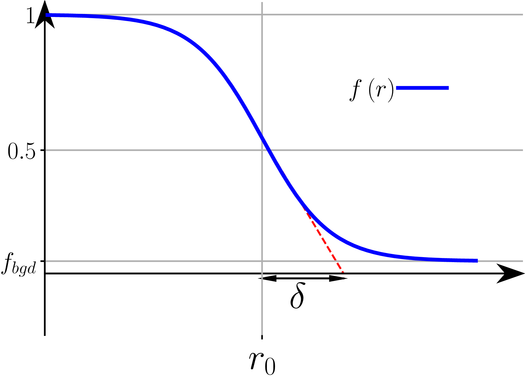


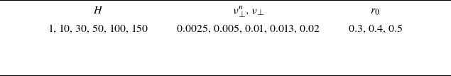


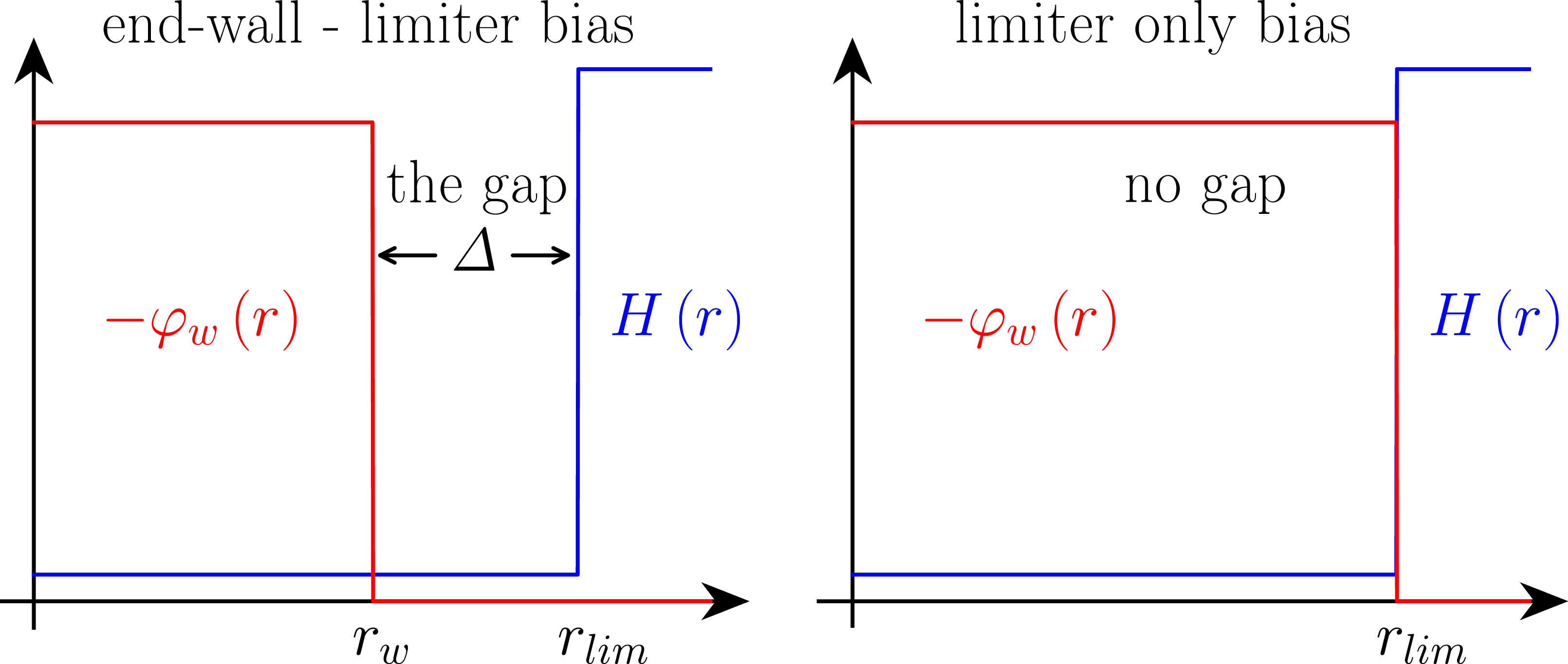


 Open access