


Introduction
Environmental factors influence echinoid distribution and abundance across spatial scales. At large scales, temperature and primary production affect larval dispersal and population distribution, while medium-to-small scales highlight the roles of wave exposure, food availability, habitat features, and human activity (Benedetti-Cecchi and Cinelli, Reference Benedetti-Cecchi and Cinelli1995; Clemente and Hernández, Reference Clemente and Hernández2008; Hernández et al., Reference Hernández, Clemente, Sangil and Brito2008; Hereu et al., Reference Hereu2012; Clemente et al., Reference Clemente, Hernández, Montaño-Moctezuma, Russell and Ebert2013). Oceanographic processes create spatial heterogeneity, with currents and physiological responses shaping large-scale distributions and local factors influencing population variability (Menge and Lubchenco, Reference Menge and Lubchenco1981; Dunson and Travis, Reference Dunson and Travis1991).
The Canary Islands located in the eastern North Atlantic lie within a Coastal Transition Zone marked by interactions between nutrient-rich coastal upwelling and nutrient-poor open-ocean waters. The archipelago’s geography, wave exposure, and mesoscale oceanographic phenomena generate gradients in temperature, nutrients, and productivity that influence marine assemblages (Barton et al., Reference Barton, Arístegui, Tett, Cantón, García-Braun, Hernández-León, Nyckjaer, Almeida, Almunia, Ballesteros, Basterretxea, Escánez, García-Weill, Hernández-Guerra, López-Laatzen, Molina, Montero, Navarro-Pérez, Rodríguez, Van Lenning, Vélez and Wild1998; Sansón et al., Reference Sansón, Reyes and Afonso-Carrillo2001; Tuya and Haroun, Reference Tuya and Haroun2009). In this region, Paracentrotus lividus occurs near the southernmost limit of its geographical range, where populations are patchier and less abundant than in temperate Atlantic or Mediterranean locations (Hernández et al., Reference Hernández, Clemente, Sangil and Brito2008; Clemente et al., Reference Clemente, Hernández, Montaño-Moctezuma, Russell and Ebert2013). These marginal conditions, characterized by strong hydrodynamics gradient and oligotrophic waters, may influence its density, feeding strategy, and ecological role.
Sea urchins, such as P. lividus, play a pivotal role in controlling algal assemblages and altering benthic community structures (Lawrence, Reference Lawrence1975; Palacin et al., Reference Palacin, Giribet, Carner, Dantart and Turo1998; Hereu, Reference Hereu2012; Hereu et al., Reference Hereu2012; Guarnieri et al., Reference Guarnieri, Bevilacqua, Figueras, Tamburello and Fraschetti2020). Their density correlates with macroalgal cover, with high densities leading to barren grounds in certain regions, although P. lividus does not form barrens in the Canary Islands (Verlaque, Reference Verlaque and Boudouresque1987; Hernández et al., Reference Hernández, Clemente, Sangil and Brito2008). Feeding strategies, such as active grazing or passive feeding on drift algae, depend on food availability (Harrold and Reed, Reference Harrold and Reed1985; Livore and Connell, Reference Livore and Connell2012), while size structure is influenced by factors like food quality, predation, and habitat complexity (Scheibling et al., Reference Scheibling, Hennigar and Balch1999; Hereu et al., Reference Hereu2012).
During the study period, the sea urchin Diadema africanum coexisted with P. lividus as the dominant herbivore on rocky shores of the Canary Islands, profoundly shaping algal assemblages and benthic community structure. However, following several large-scale mortality events attributed to disease and environmental stress (Clemente et al., Reference Clemente, Lorenzo-Morales, Mendoza, López, Sangil, Alves, Kaufmann and Hernández2014), D. africanum populations collapsed, and its ecological role has since diminished. The present work therefore provides a valuable historical reference of benthic structure and P. lividus distribution before these ecological shifts. Understanding how P. lividus persisted alongside such a dominant grazer is essential to assess functional redundancy and resilience within Canary Island benthic ecosystems.
This study investigates P. lividus populations across the Canary Islands to identify patterns in distribution and structure related to environmental factors at various scales. Specifically, it (1) examines intertidal and subtidal populations across islands and orientations, (2) characterizes algal communities, and (3) assesses small-scale habitat complexity at sampling sites.
Materials and methods
Study area
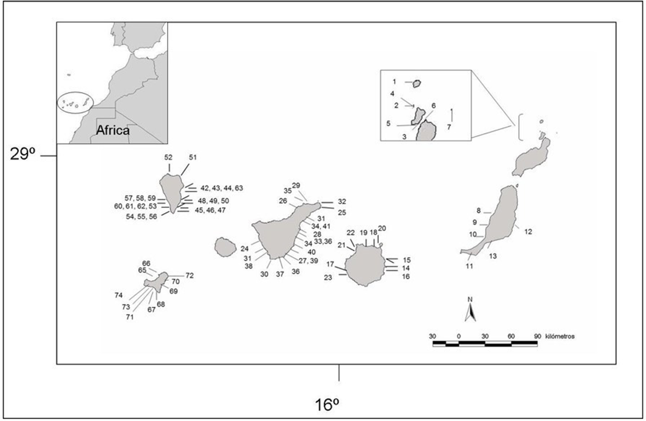
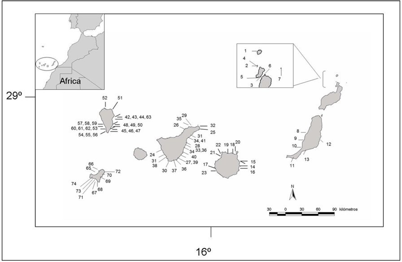
This study was conducted in the Canary Islands (NE Atlantic Ocean, 27–29° N, 13–18° W) (Figure 1), encompassing a latitudinal gradient of temperate to subtropical influence. The archipelago comprises seven main islands characterized by volcanic substrata, steep coastal profiles, and varying degrees of wave exposure. The regional oceanography is dominated by the Canary Current, producing strong upwelling along the eastern islands and a progressive westward decrease in nutrient input and productivity.
Canary Islands map with studied localities marked with numbers. Numbers may represent distinct intertidal and subtidal sites within the same locality; see Methods for details.
Sampling was performed from 2006 to 2009. Sampling effort was distributed across islands over four consecutive years (2006–2009). Not all islands were sampled each year due to weather and logistical constraints, but the relative sampling intensity among islands and habitats remained consistent throughout the study period, minimizing potential temporal biases.
A total of 103 sampling events were conducted across 84 distinct coastal locations throughout the Canary Islands. Most locations included both intertidal and subtidal habitats, which were sampled independently and thus counted as separate sampling events. A few localities, however, were sampled in only one habitat type (either intertidal or subtidal) due to accessibility or logistic constraints. Each event, therefore, represents a unique combination of locality × habitat × orientation. Locations labelled with multiple numbers on the map correspond to these paired intertidal–subtidal sites.
Field sampling
Sampling was stratified by island and wave exposure. Localities along the coast of five Islands, Fuerteventura, Gran Canaria, Tenerife, La Palma, and El Hierro, and the islets located at the north of Lanzarote Island were sampled. Fuerteventura was sampled only at intertidal habitat and Islets North Lanzarote sampled only subtidal due to logistical issues. Nonetheless, Lanzarote and Fuerteventura form a single insular entity (Carracedo, Reference Carracedo, Alfonso, Galán and Rodríguez-Martín1988).
Intertidal transects were conducted during the lowest tides of the sampling period, which in the Canary Islands occur around full and new moon phases, when tidal range is highest (up to −1 m). Sampling was restricted to low tides between −0.6 and −1 m, allowing safe access to the lower intertidal fringe. These transects were established on relatively flat rocky platforms with shallow tidepools (≈0.5 m deep). Subtidal transects were carried out at comparable depths (1–10 m) across islands and oriented parallel to the coastline on horizontal or gently sloping rocky substrates to ensure methodological consistency.
Sea urchin populations
Paracentrotus lividus’ abundance was quantified using 10 × 2 m belt transects (Hernández et al., Reference Hernández, Clemente, Sangil and Brito2008). Six to eight transects were placed at each site, depending on substrate availability, except in one case where only five were possible. All individuals of P. lividus with test diameter >2 cm were counted and measured in the field to the nearest 0.5 cm using a transparent small ruler (10 cm) placed on top of the individuals. This approach allows rapid counting and allocation to size classes, with 0.5 cm accuracy sufficient for this type of ecological study.
Multiple scales studied
Scale selection is one of the crucial determinants in ecological habitat selection studies as pointed by Mayor et al. (Reference Mayor, Schneider, Schaefer and Mahoney2009) and following its recommendations for spatial scale this study will approach the influence of each of the environmental variables separated by an objective spatial scale.
Large scale:
This is a scale separated by kilometres of distance and includes Island and orientation to wave exposure (Hernández et al., Reference Hernández, Clemente, Sangil and Brito2007; Mayor et al., Reference Mayor, Schneider, Schaefer and Mahoney2009).
- Island. At the Canary Islands Archipelago, a gradient in sea surface temperature and nutrients exists due to the influence of the North African Upwelling situated 90 km from the eastern boundary.
- Wave exposure (orientation). This variable under study depends on the orientation of the study sites with respect to oceanographic trends and is classified into three degrees of wave exposure following Yanes et al. (Reference Yanes, Marzol and Romero2006) and Hernández et al. (Reference Hernández, Clemente, Sangil and Brito2008). The first category (1), minimum degree, represents sites sheltered from both NNE dominant weather and NW swells, including the western coast of Tenerife, La Palma, El Hierro, Gran Canaria; the southeast of Fuerteventura, and the southern of the islets situated North Lanzarote. The second category (2), medium degree, includes sites exposed to dominant NE weather but sheltered from NW swells, such as eastern part of Tenerife, La Palma, El Hierro, and Gran Canaria. The third category (3), maximum degree, comprises sites exposed to both dominant NE weather and NW swells, including the northern coast of Tenerife, La Palma, El Hierro, and Gran Canaria, the western coast of Fuerteventura and northern coast of all islets situated North Lanzarote. In addition, this category also includes localities situated on headlands at the eastern coast of Gran Canaria and Tenerife which are highly exposed to NE weather.
Medium scale: Algal assemblage characterization
Along each transect, macroalgal cover (%) was assessed visually by estimating the percentage cover of dominant taxa to the nearest 5%. All taxa present at greater than 5% cover were recorded. Species included: Ellisolandia elongata (formerly Corallina elongata), Haliptilon virgatum, Jania spp., Padina pavonica, Codium spp., Ulva spp., Dasycladus vermicularis, Halopteris scoparia, Asparagopsis taxiformis, Zonaria tournefortii, Taonia atomaria, Gongolaria abies-marina, Cystoseira spp., Dyctiota spp., Sargassum spp., Gelidium spp., Pterocladiella capillacea, Lophocladia trichoclados, Lobophora canariensis, and Caulerpa racemosa. Crustose coralline algae were quantified as percentage cover, consistent with the other macroalgal taxa.
Small scale: This scale includes factors with variability in metres to centimetres (Hernández et al., Reference Hernández, Clemente, Sangil and Brito2007).
- Depth was recorded in meters deep (in positive values) only for subtidal surveys and values range 1–10 m.
- Porosity of the rock was classified based on how the lava is detached, in flows or pyroclastics. These two categories differ primarily in their porosity (Carracedo, Reference Carracedo1994). As P. lividus could dig in the rock, the type of lava is a physical variable to be considered. Flows = 1 (less porosity), compacted pyroclastics (higher porosity) = 2.
- Sedimentation (Díez et al., Reference Díez, Santolaria and Gorostiaga2003; Hernández et al., Reference Hernández, Clemente, Sangil and Brito2008; Diaz-Tapia et al., Reference Diaz-Tapia, Bárbara and Díez2013) estimated as the percentage of rock covered by sand at each transect and allocated to categories: (1) 0%; (2) 1–10%; (3) 10–20%; and (4) >20%.
-Slope (Díez et al., Reference Díez, Santolaria and Gorostiaga2003; Hernández et al., Reference Hernández, Clemente, Sangil and Brito2008) measured at each transect as the inclination of the substrate in degrees and assigned to the categories (1) 0°; (2) 0°–45°; (3) 45°–80°; and (4) 80°–90°.
- Stones: percent of big boulders and percent of small boulders by the size of their major length (L): we consider small (L < 50 cm), and large (L > 50 cm) and their percentage for each transect recorded allocated to categories: (1) 0%, (2) 0–35%, (3) 35–70%, (4) 70–100% (modified from Alves et al., Reference Alves, Chícharo, Serrão and Abreu2001; Toledo-Guedes et al., Reference Toledo-Guedes, Sánchez-Jerez, González-Lorenzo and Brito2009).
- Topographic relief (modified from McClanahan, Reference McClanahan1994; Hernández et al., Reference Hernández, Clemente, Sangil and Brito2008) described height variability along transects at scales of tens of centimetres to metres and was classified into four categories: (1) flat surface; (2) <0.25 m; (3) 0.25–0.5 m; and (4) >0.5 m relief.
- Rugosity (McCoy and Bell, Reference McCoy and Bell1991) was recorded as a finer-scale measure of surface irregularity, reflecting microhabitat complexity at the centimetre scale, and categorized as (1) flat, (2) low, (3) medium, or (4) high rugosity.
Although these last two variables describe structural complexity, they capture different spatial dimensions: high topography may result from large boulders with smooth surfaces, whereas rugosity reflects small-scale surface roughness independent of relief amplitude. Based on extensive field observations, no strong collinearity was expected between these descriptors, and both were retained as separate factors in the analysis.
Statistical analysis
Intertidal and subtidal habitats were analysed separately throughout the study because they represent ecologically distinct environments. Intertidal sites experience aerial exposure, desiccation, and thermal fluctuations, whereas subtidal sites remain permanently submerged and are influenced primarily by hydrodynamic forces and light attenuation. Environmental drivers such as wave exposure operate differently across the two habitats, and because the sampling design is not fully orthogonal or balanced, each habitat was analysed independently to avoid conflating distinct ecological processes. This approach minimizes spurious interaction effects and provides a clearer interpretation of main effects and habitat-specific responses. A previous study conducted at two representative locations during three seasons within the same year confirmed that P. lividus abundance did not differ significantly (Girard, unpublished data). Therefore, data from different sampling periods were pooled for the present analyses.
Large spatial scale
All analyses were conducted using PERMANOVA (Anderson, Reference Anderson2001) on Euclidean distance matrices of log(x + 1)-transformed data. To account for ecological and methodological differences between habitats, analyses were conducted separately for intertidal and subtidal habitats; no pooling across habitats was performed. Significant effects were followed by pairwise tests (N = number of transect included in the test).
-Island effect
To assess differences among islands, as a measure of the oceanographic gradient temperature and nutrients, island was treated as a fixed factor, and site as a random factor nested within island. Pairwise PERMANOVA tests were run following significant island effects. Intertidal (N = 326) and subtidal (N = 343).
-Wave exposure orientation
Wave exposure (three levels: low, medium, high) was treated as a fixed factor, and site as random nested within exposure. Pairwise PERMANOVA tests were run following significant wave exposure effects. Intertidal (N = 326) and subtidal (N = 343).No interaction between wave exposure or island and habitat were looked at as these operate at distinct ecological scales.
-Medium spatial scale
To explore the relationship between macroalgal cover and P. lividus abundance, we used scatterplots and linear regression. Macroalgal assemblages were identified using hierarchical cluster analysis with the unweighted pair group method with arithmetic mean (UPGMA), based on Bray–Curtis similarity.
Two PERMANOVA analyses were conducted to (1) test the effects of macroalgal assemblages and habitats on P. lividus abundance (both factors treated as fixed; N = 669) and (2) test the influence of macroalgal assemblage and habitat on P. lividus size (both factors treated as fixed; N = 489). This approach aimed to identify whether specific macroalgal assemblages promote larger urchin sizes. Transects with zero sea urchins were not used in this second analysis. Body size was analysed only at this scale because variation in size is primarily driven by local habitat complexity and food availability, not by large-scale geographic gradients.
-Small spatial scale
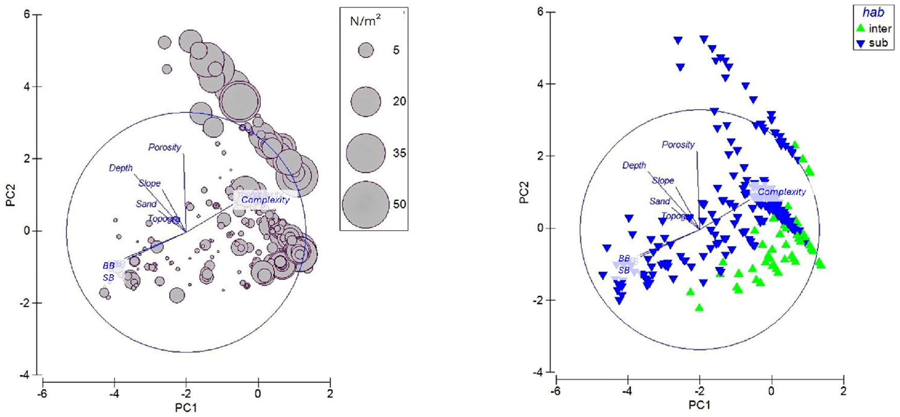
Physical descriptors of habitat complexity (depth, porosity, sedimentation, topographic relief, slope, proportion of boulders, and rugosity) were examined using principal component analysis (PCA) on normalized data (Anderson, Reference Anderson2006).
P. lividus’ abundance (N/m2) was overlaid as bubble plots to visualize associations with the main physical gradients. Principal components with eigenvalues > 1 were retained for interpretation (Chatfield and Collins, Reference Chatfield and Collins1983). Analyses were based on balanced designs and log(x + 1)-transformed data to minimize heterogeneity of dispersion among groups.
Results
Influence of large spatial scale variables: islands and orientations
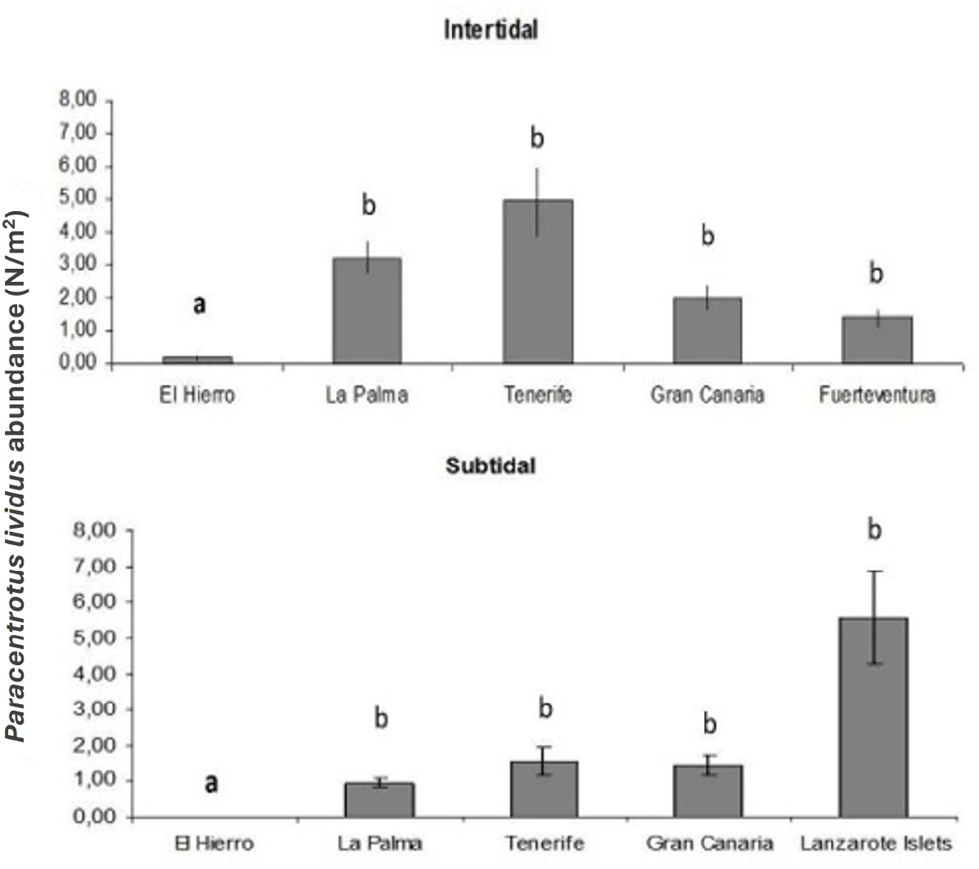
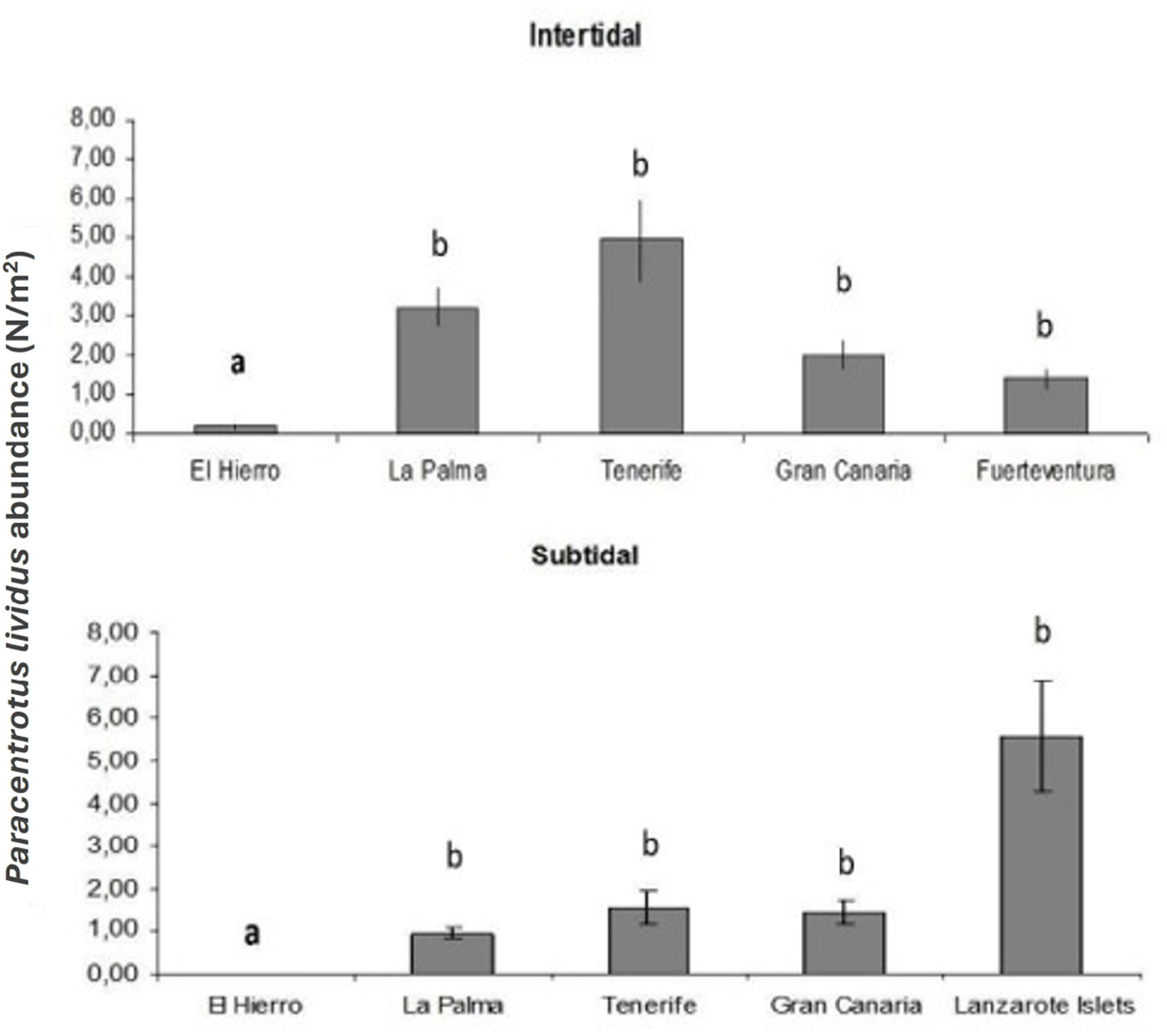
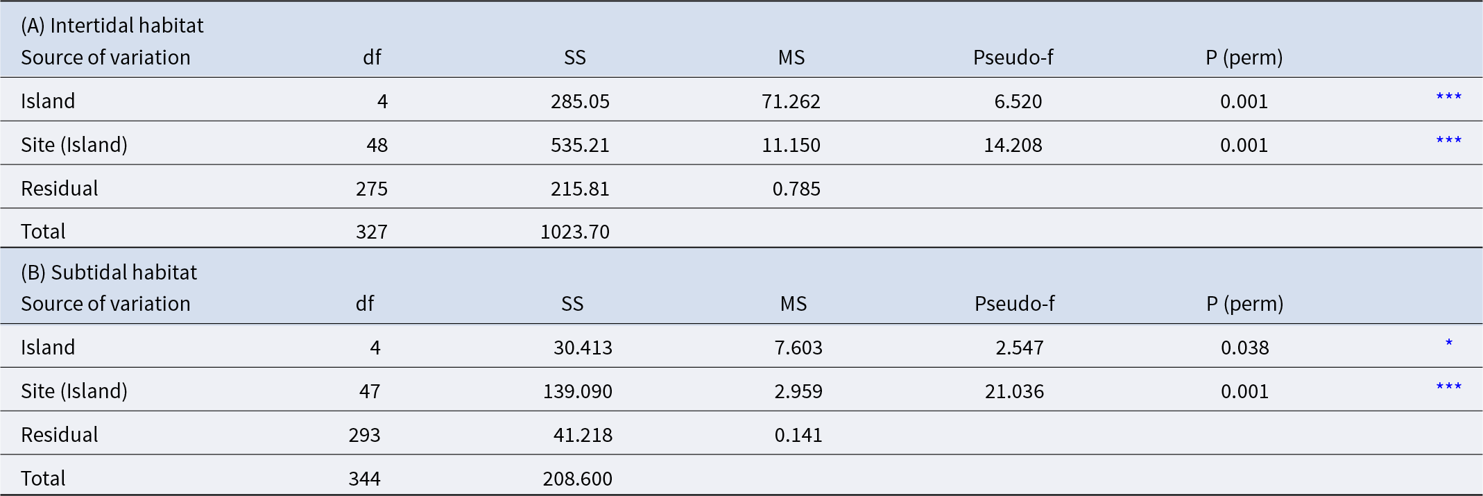
Islands have different abundances of Paracentrotus lividus both at intertidal (F = 6.52, p < 0.001) and subtidal (F = 3.903, p < 0.05) habitats (Table 1 and Figure 2). Differences between El Hierro (westernmost Island) and any of the other Canary Islands are significant for both habitats (p < 0.01).
Mean abundance of Paracentrotus lividus (N/m2) for each Island. Error bars represent SE. Different letters identify groups significantly different (p < 0.05).
Results of the PERMANOVA analysis for Paracentrotus lividus abundance among different islands and localities: (A) intertidal habitat and (B) subtidal habitat
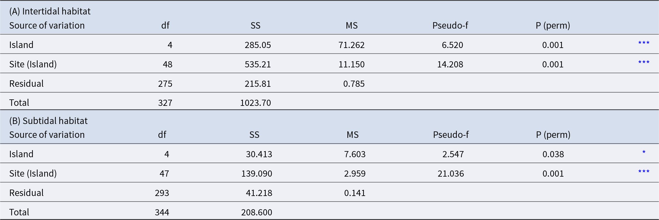
* p < 0.05,
*** p < 0.001.
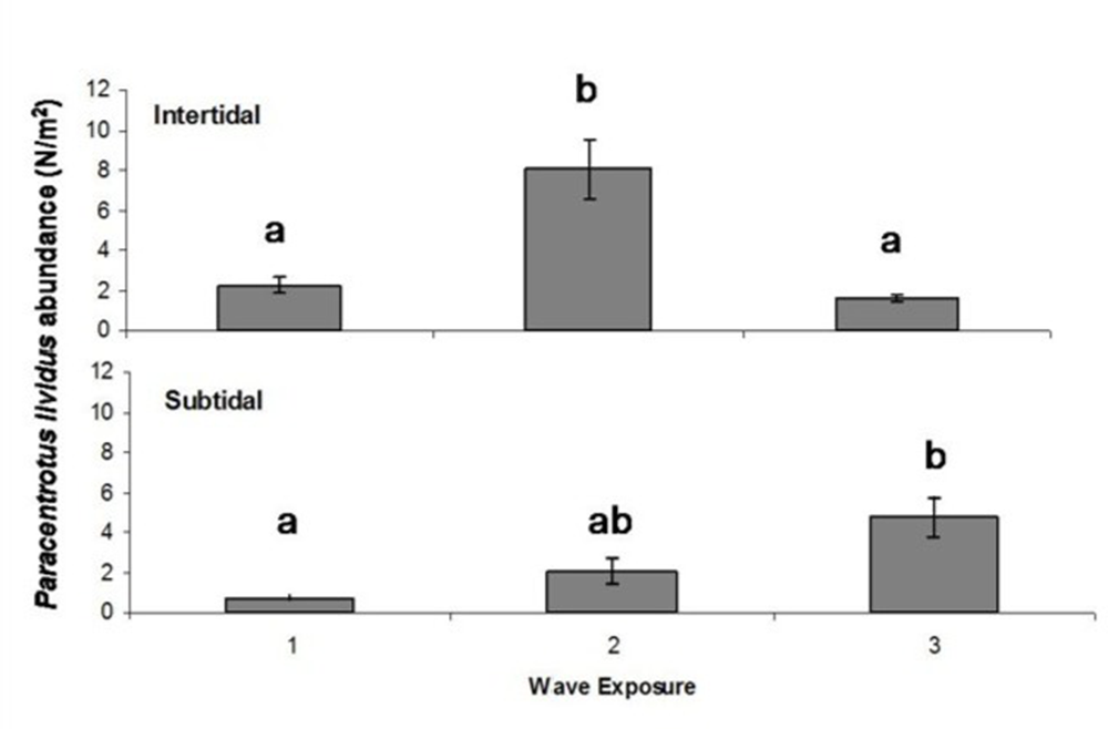
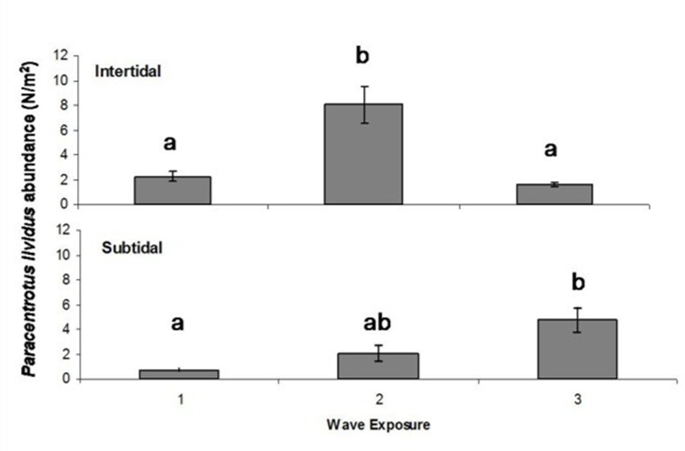
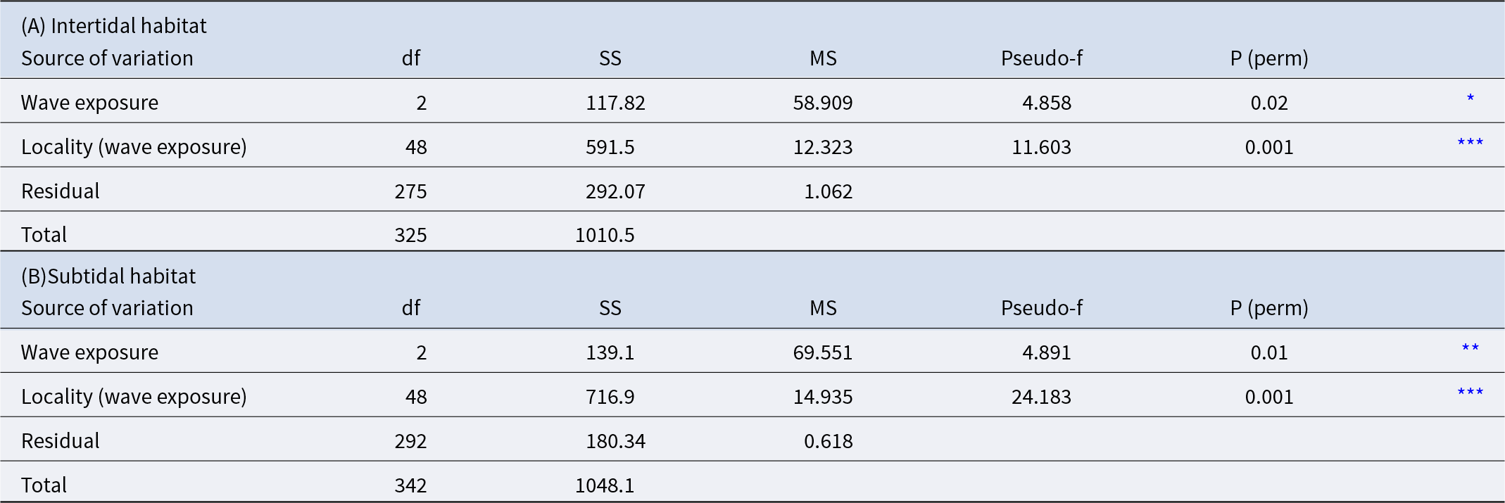
P. lividus population was significantly different depending on wave exposure for both intertidal and subtidal habitat (Table 2 and Figure 3). For the intertidal habitat, populations at sheltered sites (2.25 ± 0.42 ind./m2) did not differ in abundance from those at highly exposed sites, but both were significantly lower than populations at intermediate exposure (8.07 ± 1.47 ind./m2). In contrast, in the subtidal habitat, abundance at sheltered sites (0.73 ± 0.14 ind./m2) was significantly lower than at highly exposed sites (4.81 ± 0.99 ind./m2), while populations at intermediate exposure (2.08 ± 0.56 ind./m2) did not differ significantly from either.
Abundance of Paracentrotus lividus in intertidal and subtidal habitats across three levels of wave exposure: 1 = sheltered, 2 = intermediate, 3 = highly exposed. Error bars represent SE. Different letters identify groups significantly different (p < 0.05).
Results of the PERMANOVA analysis for Paracentrotus lividus abundance among different wave exposure and localities: (A) intertidal habitat and (B) subtidal habitat
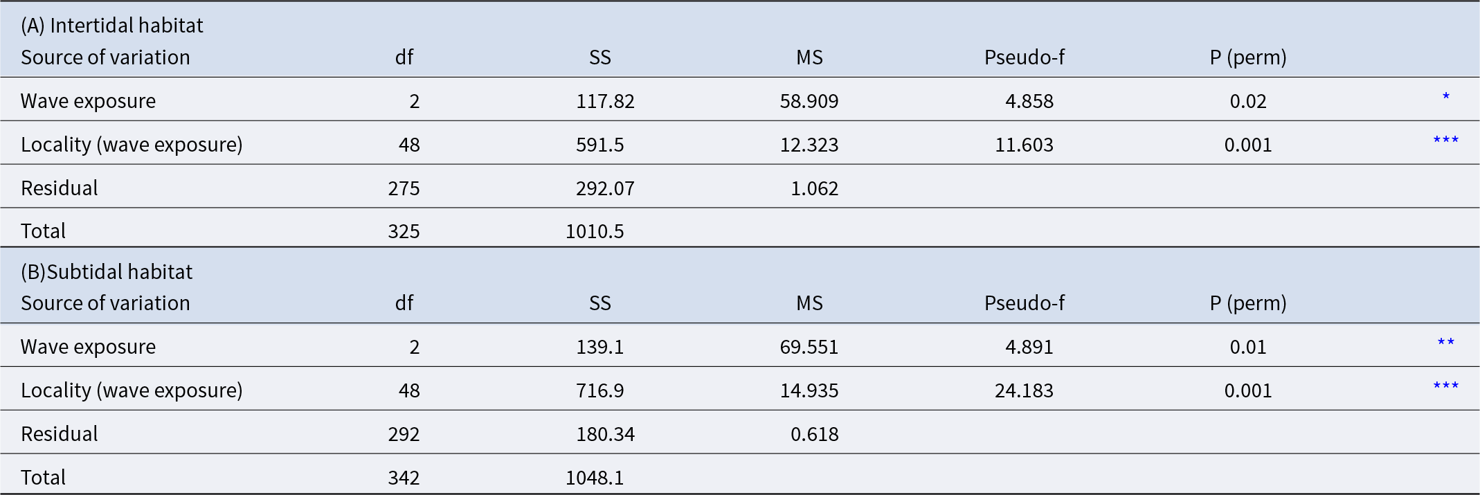
ns = not significant;
* p < 0.05,
** p < 0.01,
*** p < 0.001.
Influence of medium spatial scale variables: macroalgae environment
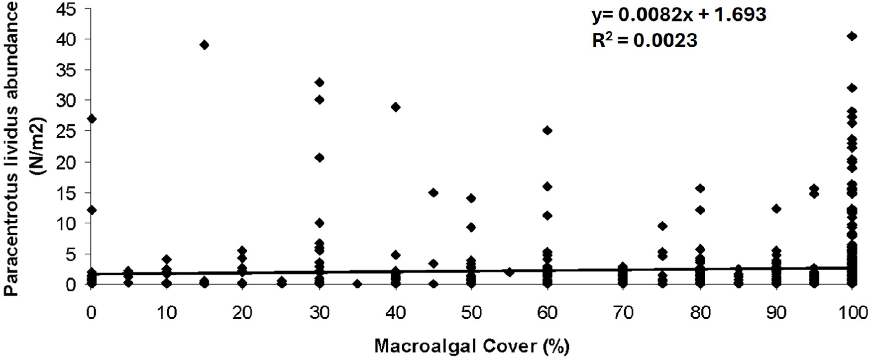
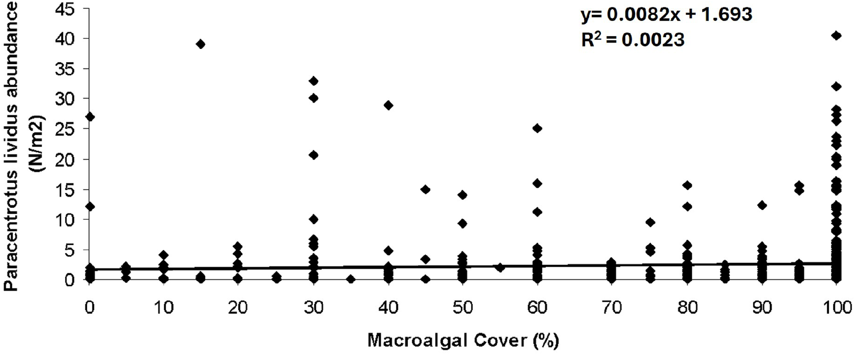
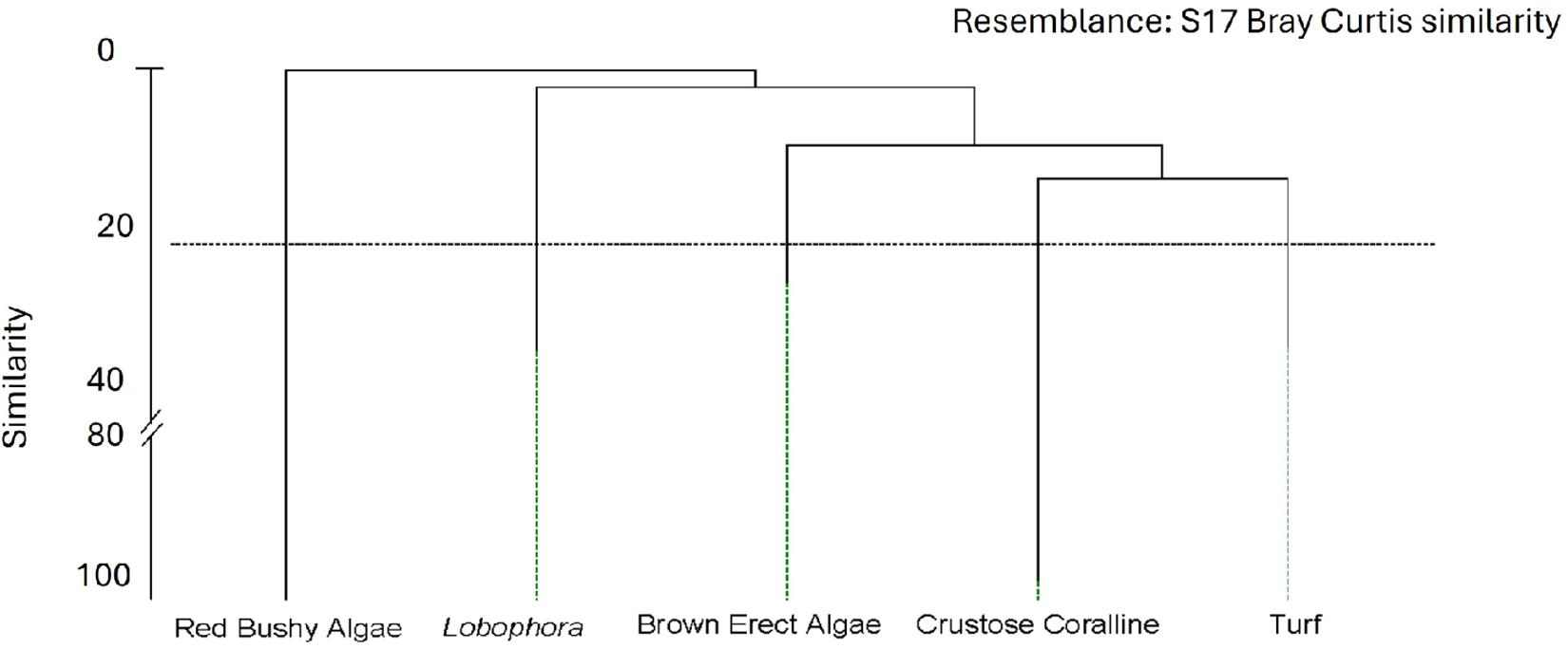
No relationship was found between P. lividus abundance and the macroalgal cover (Figure 4). Regarding macroalgae specific composition, the UPGMA dendrogram based on Bray–Curtis similarity correctly grouped sites according to macroalgal composition (Figure 5). Analyses were performed on a matrix of samples (transects) × macroalgal taxa, subsequently grouped into the 13 dominant species identified by similarity percentage analysis (SIMPER), which determines the taxa contributing most to Bray–Curtis similarity patterns. Clusters represented sites sharing similar assemblage structure.
Scatter plot representing abundance of Paracentrotus lividus (N/m2) vs. macroalgal cover (%). No linear relationship is found (R2 = 0.0023).
Cluster grouping algae species. UPGMA analysis based on a matrix of samples (transects) × macroalgal taxa, subsequently grouped into 5 main groups through SIMPER (Cut at Bray Curtis similarity = 20%).
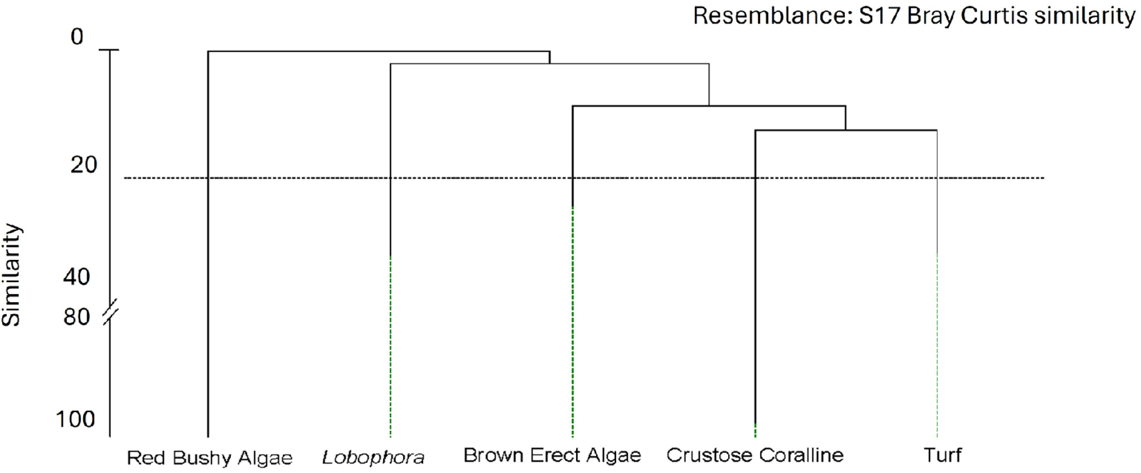
The cluster (Figure 5) grouped the sampling sites based on their algal composition with a similarity of 20% in five main algal assemblages. We considered this level adequate as it explains the same as partitions at higher similarities. The first group, from now on named as Turf, is formed by short thallus algae, mainly Jania virgata (syn. Haliptilon virgatum), Jania spp., Ellisolandia elongata (formerly Corallina elongata), Dyctiota spp., and Halopteris scoparia. The second group is dominated by erect algae with bigger thallus, mainly brown algae: Cystoseira spp., Gongolaria abies-marina, and Sargassum desfontainensis and to a lesser extent by Asparagopsis taxiformis. The third group is characteristic of red bushy algae formed principally by Gelidium spp. and Lophocladia trichocladus. The fourth group is monospecific, Lobophora canariensis, which dominates wherever it appears. The last group is formed by a compound of crustose corallines characteristic of barren areas. The rest of the surveyed species were eliminated since their contribution was less than 7% of the similarity for each group.
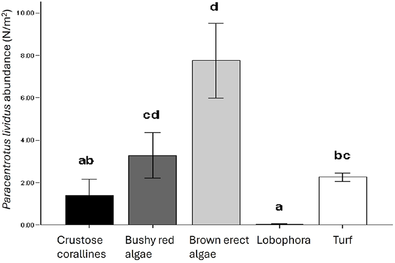
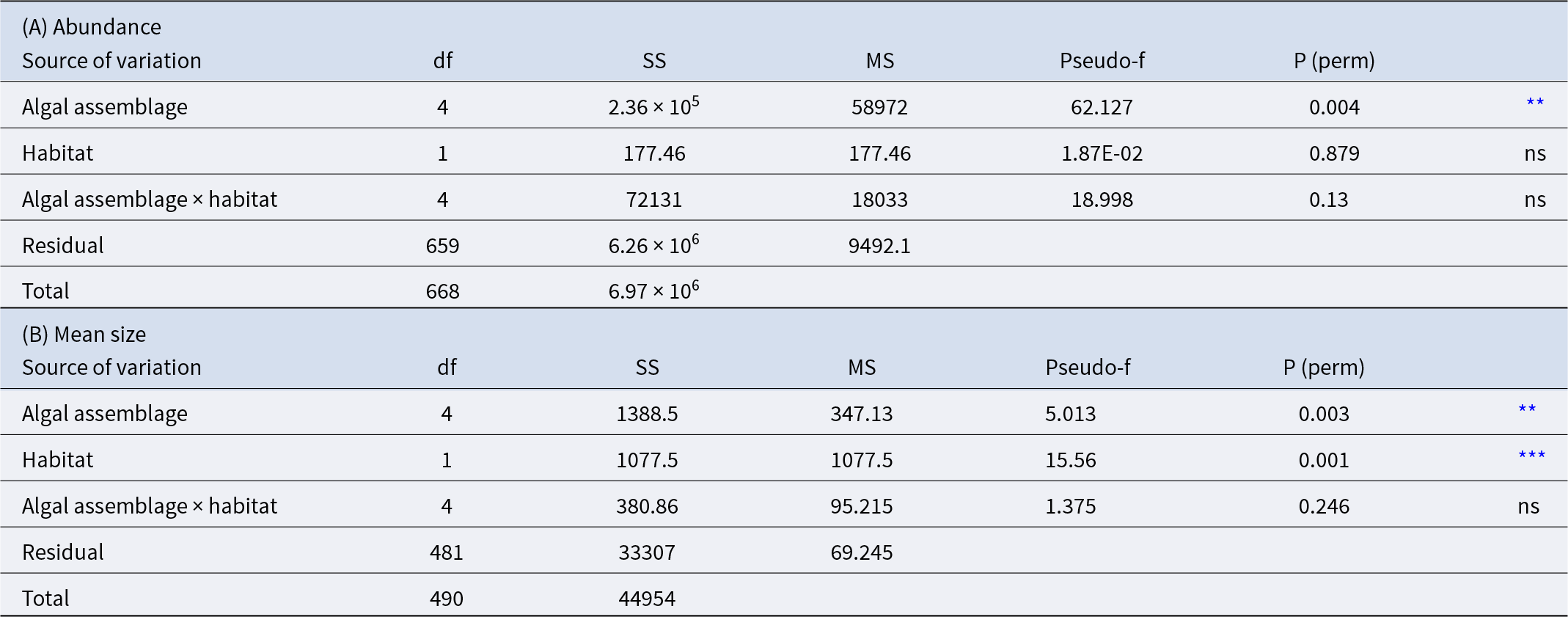
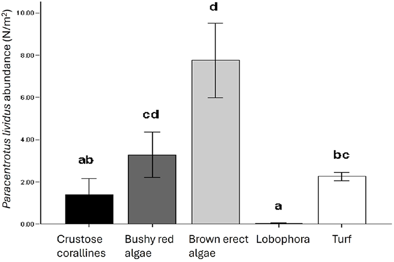
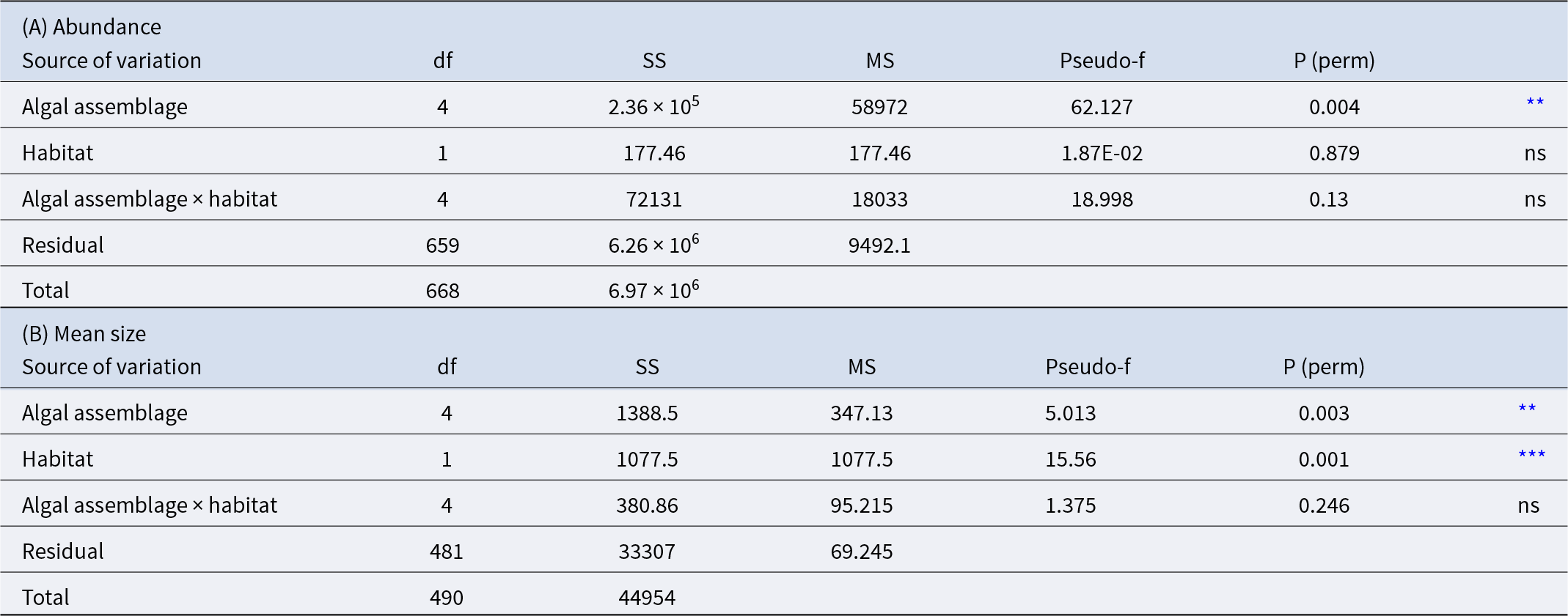
P. lividus’ abundance was found to be influenced only by the algal assemblage group and not depends on the habitat (inter- or subtidal) (Table 3A and Figure 6). The alga Lobophora canariensis seems to have a negative effect on sea urchin population, where Lobophora is present very few or no P. lividus was found (0.042 ± 0.017 N/m2). At the other extreme, in brown erect algal assemblages, P. lividus is more abundant (7.749 ± 1.772 N/m2). The other assemblages (red bushy algae, turf, and crustose corallines) showed intermediate values (3.285 ± 1.072; 2.254 ± 0.206; 1.378 ± 0.782 N/m2 respectively) (Figure 6).
Bar charts represent Paracentrotus lividus abundance (N/m2) in each macroalgal assemblage. Error bars represent SE. Different letters identify groups significantly different (p < 0.05).
(A) Results of the PERMANOVA analysis for Paracentrotus lividus abundance among different algal assemblages and habitats. (B) Results of the PERMANOVA analysis for P. lividus mean size upon different algal assemblages and habitats
ns = not significant;
** p < 0.01,
*** p < 0.001.
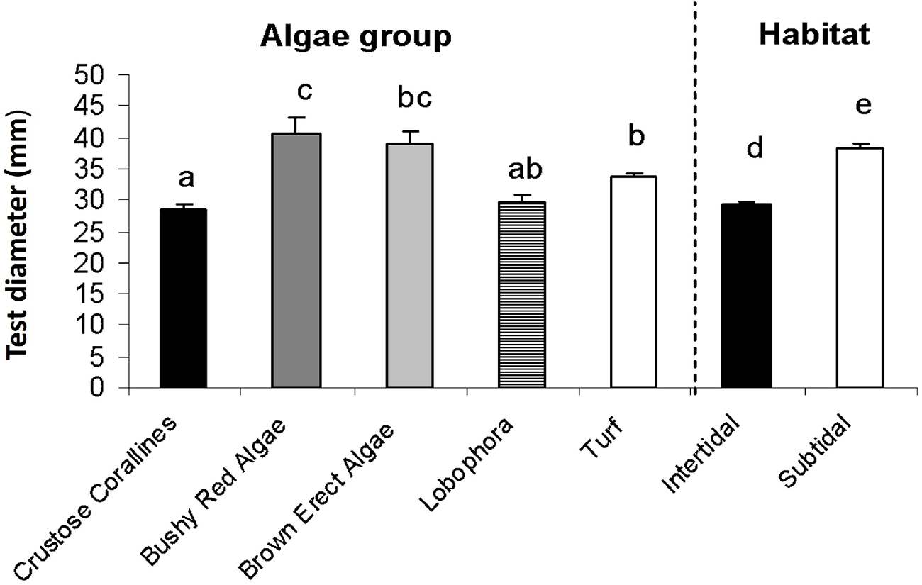
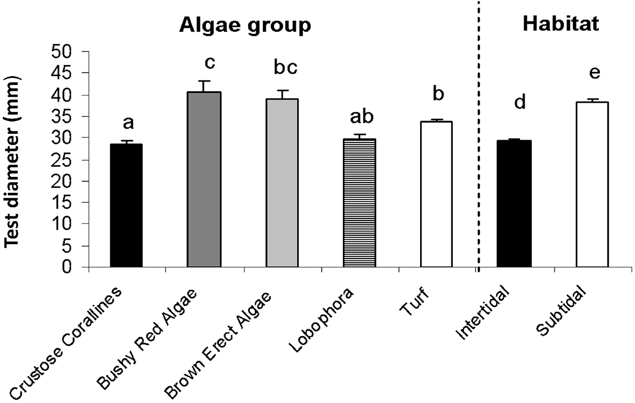
P. lividus mean size resulted to be influenced by both the algal assemblage (p < 0.01) and the habitat (intertidal or subtidal) (p < 0.001) and no interactions were detected (Table 3B and Figure 7). Sea urchins living underwater are bigger (mean size intertidal individuals = 29.183 ± 0.414 mm and mean size subtidal individuals = 38.397 ± 0.642 mm). P. lividus sea urchins living in bushy red and brown erect algae were bigger (40.546 ± 2.689 mm, 38.995 ± 2.010 mm, respectively) than those living in crustose corallines (28.395 ± 0.840 mm) (Figure 7).
Bar charts represent Paracentrotus lividus mean test diameter (mm) for each macroalgal assemblage (left of the dotted line) and for each habitat (right of the dotted line). Error bars represent SE. Different letters indicate statistically significant differences among groups (p < 0.05).
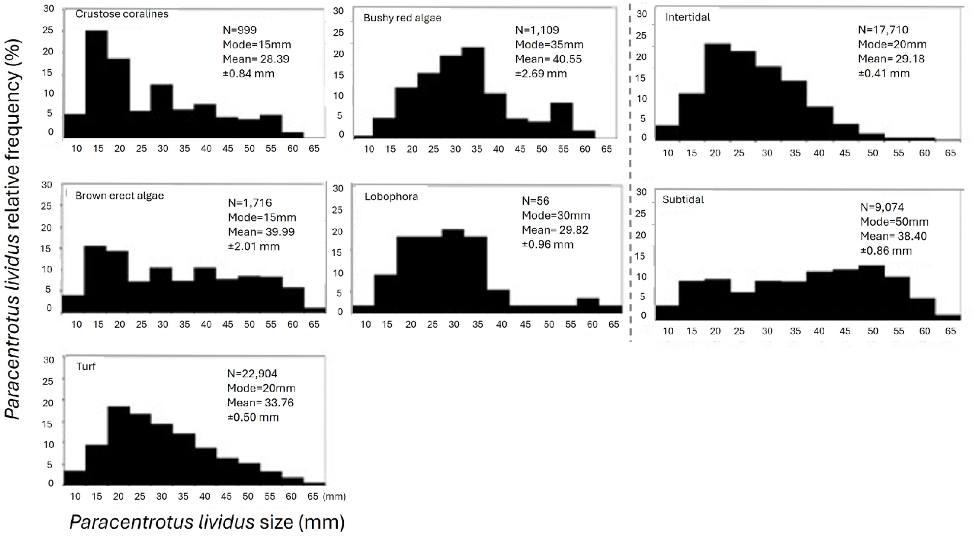
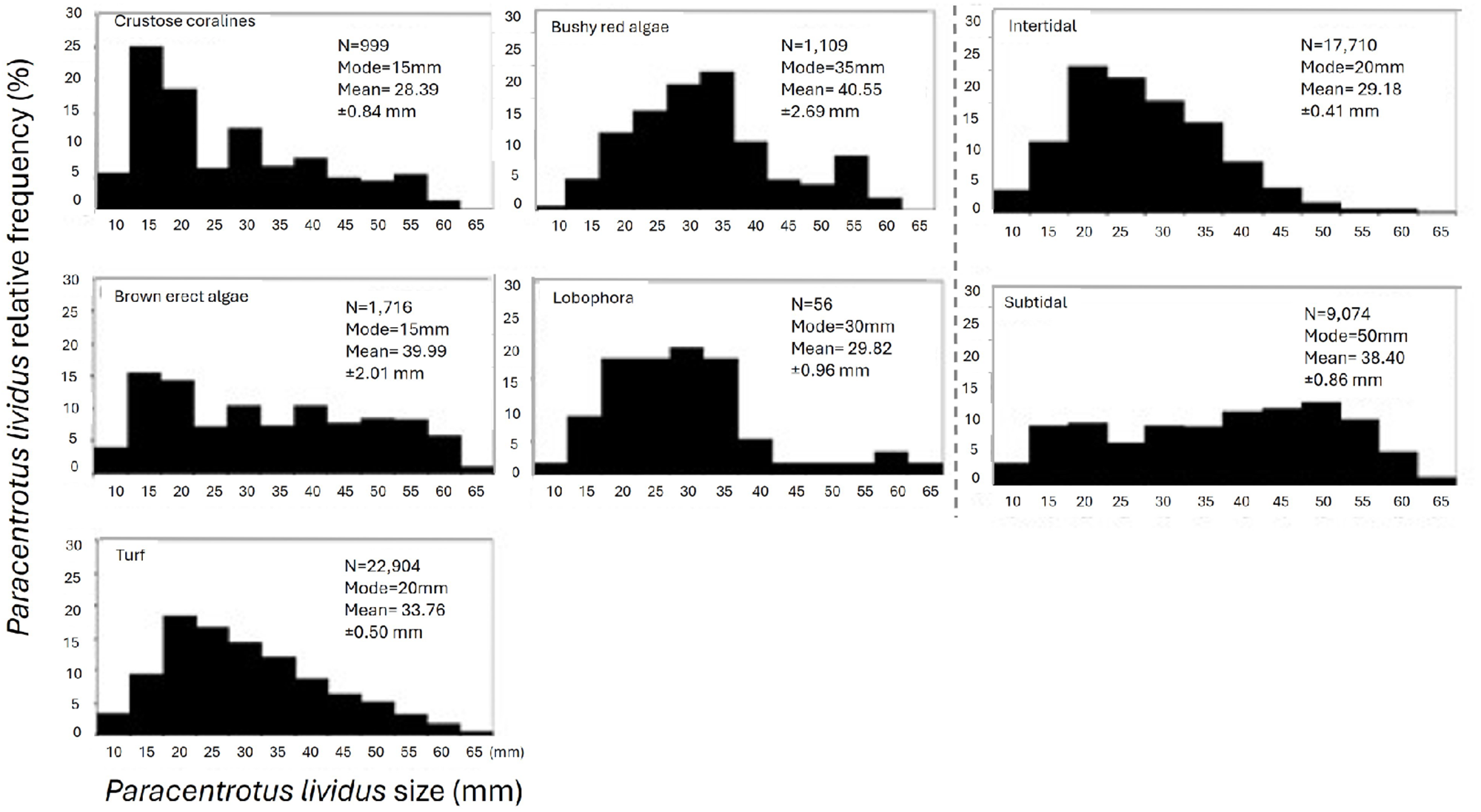
The size structure for intertidal populations is skewed to smaller sizes (mode = 20 mm), while subtidal habitats have a larger mode (50 mm), and size distribution more homogeneous (Figure 8). Crustose corallines and brown erect algal assemblages have low modes (15 mm); however, in crustose corallines, the sea urchins had a small mean size (28.39 mm) while urchins living in brown erect algae had a much higher mean size (39.99 mm) than its mode, and therefore, its distribution is more homogeneous throughout all the size classes. The higher mode was observed in red bushy algal assemblage (35 mm) followed by Lobophora canariensis (30 mm). Urchins living in the turf assemblage had a very pronounced size structure and registered a mode skewed to small individuals (20 mm).
Size structure for pooled samples of Paracentrotus lividus at different algal assemblages (left of the dotted line) and at different habitat, intertidal or subtidal (right of the dotted line). Size interval is 5 mm.
Influence of small spatial scale variables: habitat complexity
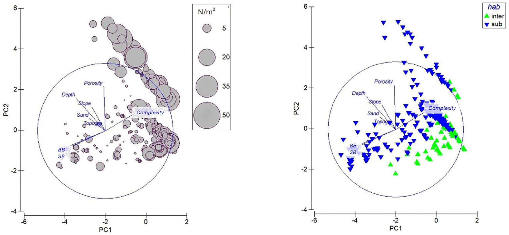
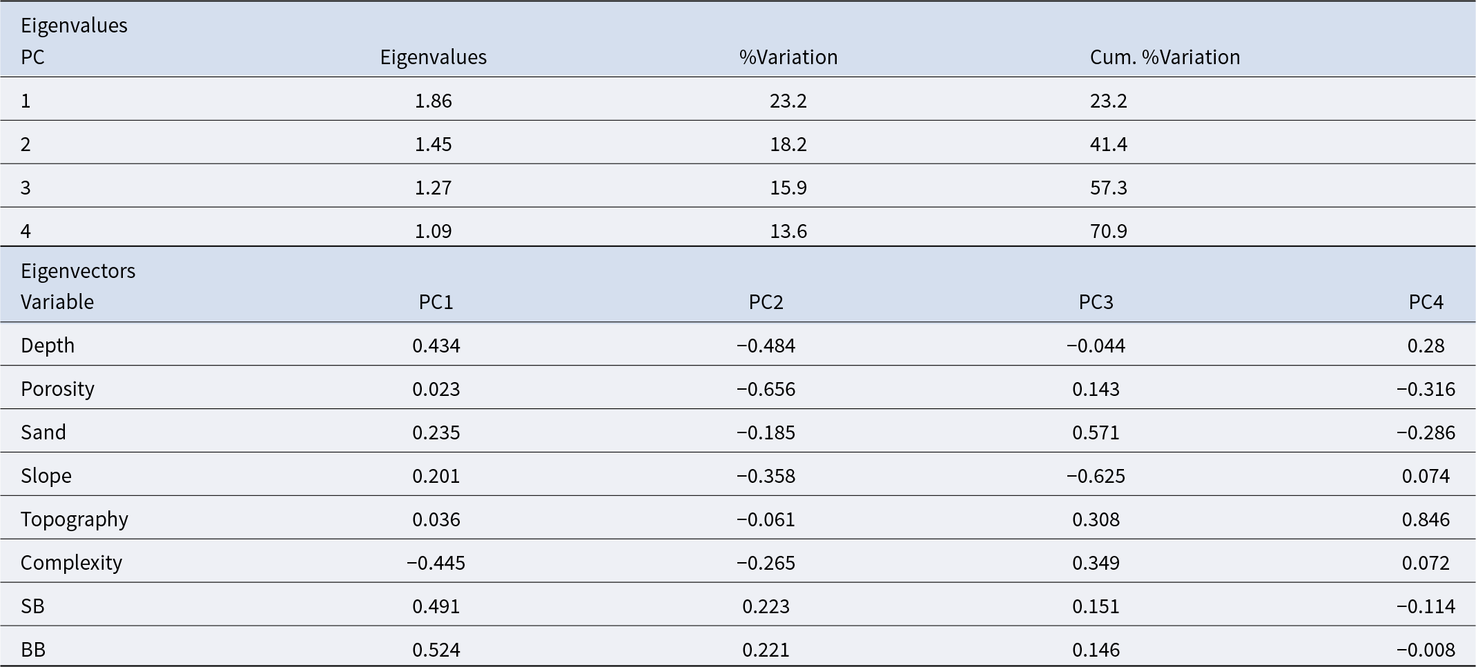
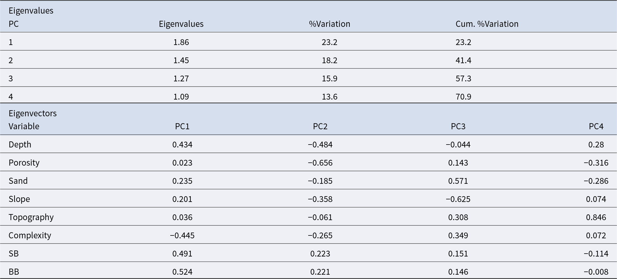
P. lividus abundance is positively influenced by the substratum porosity and complexity and is scarce at boulders areas (Figure 9 and Table 4). PCA explains up to 41.4% of sample variability with two axis and up to 57.3% with the third axis. The highest abundance of P. lividus was found at sites characterized by white rough-type porous rock and higher complexity. By other hand, boulders (small and big) are less suitable characteristics for both habitats (intertidal and subtidal) (Figure 9). By contrast, slope has a negative effect on the abundance of P. lividus at intertidal surveys but not at subtidal ones, where it has a small positive relation (Figure 9).
Principal components analysis (PCA) explaining the abundance of Paracentrotus lividus through small scale physical variables: depth, porosity of the rock, sand, topographic relief, slope, boulders and habitat complexity. A) Bubbles represent abundance of P. lividus (N/m2). B) Samples are labelled by factor habitat (hab): green intertidal and blue subtidal.
Eigenvalues and variable loadings for the first four principal components (PC1–PC4) from a PCA of small-scale physical variables. Eigenvalues indicate the variance explained by each component, and loadings represent the contribution of each variable to the respective PC
Although sand bottom is not a suitable substratum for sea urchins, the relation between P. lividus and the amount of sand was not significant either for intertidal or subtidal areas (Table 4), but it can be appreciated on the PCA plots, how bigger bubbles, representing P. lividus higher abundance, are segregated to low or absence of sand (Figure 9).
At intertidal habitat, the substratum’s porosity and habitat complexity are positively correlated with the abundance of P. lividus, while slope is negatively correlated. At the subtidal habitat, the porosity of the rock continues to be the most correlated variable while the slope happens to be opposite correlated positively with the abundance of P. lividus together with topographic relief, that is also negatively correlated (Figure 9).
Discussion
This study provides a broad-scale description of the spatial distribution and abundance patterns of Paracentrotus lividus across the Canary Islands, based on an extensive and geographically representative dataset. The results reveal marked variability among islands and between habitats, suggesting that both large- and small-scale environmental factors contribute to shaping the species’ population structure in the region.
At a large spatial scale, there appears to be variability in the abundance of P. lividus across the Canary Islands. Although only El Hierro is significantly different from others, there is a trend of greater abundance of P. lividus in subtidal populations of the western islands, which are closer to the African upwelling. These islands are characterized by colder water and higher productivity, which provide optimal conditions for this temperate species. However, this pattern from west to east is less evident in intertidal populations, where higher abundance of P. lividus is observed in the intertidal zones of Tenerife and La Palma than in eastern islands. Although this result may be biased by differences in sampling effort, it is remarkable that both central islands, Tenerife and Gran Canaria have high abundance on intertidal populations, which could be influenced by anthropogenic impact, given that they are the most populated islands. To obtain a more comprehensive understanding of the potential effects of human activity upon intertidal communities in the Canary Islands, more systematic and thorough sampling efforts are needed. Nonetheless, it is evident that P. lividus is negligible at the westernmost island of El Hierro, while it is more abundant as we move east.
Smaller scale variables could be connected and might play an important role explaining the abundance differences between islands. Abundance of P. lividus at intertidal areas of the eastern island Fuerteventura is lower than abundances at central islands. This trend may be attributed to the fact that Fuerteventura is the sandier island, and sand has been shown to be a less suitable substratum for sea urchin survival. As a result, intertidal habitats in the central and eastern islands with a more favourable combination of small-scale physical characteristics appear to be more suitable for this species.
The influence of wave exposure on sea urchin P. lividus populations varies between habitats, intertidal and subtidal. Although seemingly contradictory, we propose that this difference can be explained. Sea urchins in the intertidal habitat are less abundant in sheltered areas due to increased vulnerability to anthropogenic activities, such as harvesting and destruction by other anthropogenic activities as they result inconvenient for beachgoers. Moderate wave exposure may limit these pressures, whereas high hydrodynamics can exceed the species’ attachment threshold, as demonstrated in previous studies (Tuya et al., Reference Tuya, Cisneros-Aguirre, Ortega-Borges and Haroun2007). Conversely, in the subtidal habitat, P. lividus shows a progressive increase in abundance from sheltered to highly exposed areas. Unlike the intertidal, this habitat is more stable and receives less direct wave impact, which may explain the presence of larger and more abundant urchins at the most exposed sites. In these locations, post-swell accumulations of drift algae are also more common, potentially sustaining these denser populations. This supports the idea of subsiding feeding in these habitats, as suggested by Harrold and Reed (Reference Harrold and Reed1985) and Britton-Simmons et al. (Reference Britton-Simmons, Foley and Okamoto2009).
At medium scale, the abundance of the common European sea urchin, P. lividus, in the Canary Islands showed no relationship with the total macroalgal cover. However, according to the algal groups identified in this study, the abundance of P. lividus is influenced by the algal assemblage where it lives; it is higher in those places with algal assemblages dominated by Gongolaria spp., Sargassum spp., Laurencia spp., and Gelidium spp. These algae are typical in exposed coasts, principally north coasts of the Islands (Sangil et al., Reference Sangil, Sansón and Afonso-Carrillo2011) where commonly higher productivity are present due to strong mixing events (Arístegui et al., Reference Arístegui, Hernández León, Gómez, Medina, Ojeda and Torres1989) and generate drift algae accumulations after swell storms. Although diet studies should be performed to demonstrate passive feeding, it seems P. lividus abundance is related with assemblages that produce drift accumulations and individuals of P. lividus found at these assemblages are also significantly bigger. Wave exposure, as hypothesized, highly influences population size of sea urchins, and it does it in a different way for each habitat.
Sea urchins and macroalgae have been correlated negatively in many studies: Sangil et al. (Reference Sangil, Sansón and Afonso-Carrillo2011) found that sea urchin density explains the highest variation in algal assemblages across the Canary Islands, Hernández et al. (Reference Hernández, Clemente, Sangil and Brito2008) found negative correlation between macroalgal assemblages and Diadema africanum populations off Canarian coasts, and Guidetti and Dulcić (Reference Guidetti and Dulcić2007) found positive correlations between P. lividus and Arbacia lixula with the extend of barrens in the Mediterranean. However, for P. lividus, there is no negative correlation with macroalgae species (except for Lobophora canariensis). Harrold and Reed (Reference Harrold and Reed1985) and Vanderklift and Kendrick (Reference Vanderklift and Kendrick2005) studied populations of sea urchins and found that when drift algae are available, urchin grazing is minimized and little effect upon attached algae exists. If we assume that drift algae are an important resource for Canarian P. lividus, it seems it is the algal assemblage which determines the abundance and size of its populations, since no grazing effect is manifest. Moreover, we can conclude that wave exposure is a key determinant of P. lividus abundance in both intertidal and subtidal habitats, as drift-forming algae are more abundant on the exposed coasts of the Canary Islands (Cabrera González, Reference Cabrera González2016).
Cystoseira sensu lato species are brown erect algae capable to generate drift and includes three genera Cystoseira, Ericaria, and Gongolaria. Species of Cystoseira s.l. in the Canary Islands are more abundant in Northern and North-Eastern areas and are more abundant in the Eastern Islands (Sangil et al., Reference Sangil, Sansón and Afonso-Carrillo2011), the geographical distribution of 80% of this genus is North Atlantic and Mediterranean coasts (Oliveras-Plá and Gómez Garreta, Reference Oliveras-Plá and Gómez Garreta1989), the same distribution as P. lividus (Boudouresque and Verlaque, Reference Boudouresque, Verlaque and Lawrence2007), so it seems reasonable that where this algal assemblage dominates, P. lividus will also find its optimal environmental conditions, as our results support. In the opposite, the algal assemblage negatively correlated with P. lividus’ abundance; Lobophora canariensis, which has tropical affinities (Brito, Reference Brito and Afonso-Carrillo2008; Metian and Warnau, Reference Metian and Warnau2008), appeared in the southeasternmost island: El Hierro, in concordance with Sangil et al. (Reference Sangil, Sansón and Afonso-Carrillo2011), and in calm and warm waters (South and southwest of Tenerife and Gran Canaria and West of La Palma). It is also remarkable that L. canariensis although has plasticity to generate different forms (Haroun et al., Reference Haroun, Gil-Rodríguez, De la Torre and Canseco2003), it usually grows forming a dense mat that covers the substrate and could reduce the survivorship of newly settled sea urchins (Hernández et al., Reference Hernández, Clemente, Sangil and Brito2008) and making it difficult for other species, including other herbivores, to colonize (Haroun et al., Reference Haroun, Gil-Rodríguez, De la Torre and Canseco2003).
Individuals of P. lividus in the intertidal zone tend to be smaller, as previously reported by Haya de la Sierra (Reference Haya de la Sierra1990) andGonzález-Irusta (Reference González-Irusta2009), which may reflect higher mortality rates in this habitat. Several factors could contribute to this pattern, including increased physiological stress or human disturbance. As observed previously in the Canary Islands, a mortality event caused by bald sea urchin disease particularly affected large P. lividus individuals in intertidal areas along the south coast of Tenerife (Girard et al., Reference Girard, Clemente, Toledo-Guedes, Brito and Hernandez2012). Although González-Irusta (Reference González-Irusta2009) identified human harvesting as a relevant factor, this activity is of minor importance in the Canary Islands, where sea urchin collection is not a widespread practice.
Predation pressure has been widely recognized as a key driver of sea urchin density and size structure (Sala and Zabala, Reference Sala and Zabala1996; Gianguzza et al., Reference Gianguzza, Chiantore, Bonaviri, Cattaneo-Vietti, Vielmini and Riggio2006; Guidetti, Reference Guidetti2006; Ceccherelli et al., Reference Ceccherelli, Pinna and Sechi2009; Clemente et al., Reference Clemente, Hernández and Brito2009). Natural predation in the intertidal is generally weaker than in the subtidal zone, where it is exerted mainly by the sea star Coscinasterias tenuispina and by the fishes Thalassoma pavo, Diplodus sargus, and D. cervinus (Clemente, Reference Clemente2007). In the subtidal, predation tends to act more strongly on small individuals (Guidetti, Reference Guidetti2004). Differences in size distribution may also be influenced by population density (Levitan, Reference Levitan1989), settlement rates (Barnes and Crook, Reference Barnes and Crook2001; Tomas et al., Reference Tomas, Romero and Turon2004), and migration processes (Fernandez et al., Reference Fernandez, Caltagione and Johnson2001; Hereu, Reference Hereu2004; Ceccherelli et al., Reference Ceccherelli, Pinna and Sechi2009).
At the small spatial scale, habitat complexity emerged as a key determinant of P. lividus distribution, with substrate complexity and rock porosity identified as the most influential variables. Structural complexity has been highlighted in previous studies as an important factor enhancing survival, as it provides shelter from predators (Hereu et al., Reference Hereu, Zabala, Linares and Sala2005). Similarly, the porosity of the rock allows P. lividus to excavate refuges, thereby increasing protection from predation and hydrodynamic stress (Cuenca, Reference Cuenca1987; Jacinto et al., Reference Jacinto, Bulleri, Benedetti-Cecchi and Cruz2013).
P. lividus populations in Canary Islands seem to function in a different way as the same species in the Mediterranean, where high densities transform macroalgal communities into barren grounds (Palacin et al., Reference Palacin, Giribet, Carner, Dantart and Turo1998; Ruitton et al., Reference Ruitton, Francour and Boudouresque2000; Bulleri et al., Reference Bulleri, Bertocci and Micheli2002), since it appears unable to transform benthic coastal macroalgal communities. Instead, it seems that the only echinoid species that during the studied period played this role in the Archipelago was Diadema africanum (Hernández et al., Reference Hernández, Clemente, Sangil and Brito2007, Reference Hernández, Clemente, Sangil and Brito2008). In this Archipelago, P. lividus’ substrate availability was restricted by D. africanum and would be more abundant in areas where hydrodynamic conditions are high and D. africanum cannot live (Tuya et al., Reference Tuya, Cisneros-Aguirre, Ortega-Borges and Haroun2007). P. lividus is a border species in this area and does not seem to be competent enough to gain territory when competing with D. africanum, which restricted its distribution not only in bathymetry but also in the ecological role that P. lividus usually plays, structuring algal assemblages, at other latitudes.
Border species are especially sensitive to environmental changes (Parmesan, Reference Parmesan1996; Berteness et al., Reference Berteness, Leonard, Levine and Bruno1999; Case et al., Reference Case, Holt, McPeek and Keitt2005; Parmesan et al., Reference Parmesan, Gaines, Gonzalez, Kaufman, Kingsolver, Peterson and Sagarin2005), and so the fact that this species is living at its southernmost geographical limit is likely to be related to its ecology. In Canary Islands, it is the macroalgal assemblage which determines the abundance and size structure of P. lividus, and therefore in a global warming scenario, the tropicalization of the flora in this Archipelago (Brito, Reference Brito and Afonso-Carrillo2008) would benefit algae with tropical affinities, as Lobophora canariensis, that is starting to gain space. In contrast, Cystoseira s.l. and specially Gongolaria abies-marina ecosystem seem to be in regression (Brito, Reference Brito and Afonso-Carrillo2008; Martin et al., Reference Martin, Rancel-Rodríguez, Sangil, Reyes, Benito, Orellana and Sansón2022) and this could affect P. lividus distribution. Comparison of this historical dataset with current population and habitat data across the archipelago will contribute to understanding long-term changes in P. lividus distribution and the ecological drivers shaping its dynamics under accelerating environmental change.
Author contributions
D.G. conceived and designed the study, carried out the fieldwork, analysed the data, and wrote the manuscript. J.C.H. supervised the study, contributed to the development of the study design and statistical analyses, and provided critical revisions of the manuscript. Both authors approved the final version of the manuscript.
Funding
This study was supported by a research project funded by the Junta Nacional Asesora de Cultivos Marinos (JACUMAR), Ministerio de Agricultura y Pesca, Spain.
Competing interests
The authors declare no conflict of interests.
Ethical standards
All field sampling was conducted in accordance with local regulations and ethical standards applicable at the time of the study.
Data availability
The data that support the findings of this study are not publicly available but are available from the corresponding author upon request for scientific purpose.

 Open access

