


1. Introduction
Lipid bilayers constitute the fundamental structural components of biological membranes. They separate the cell from its exterior and organelles from the cytoplasm. In order to support life, they must balance the competing demands of fluidity versus mechanical robustness and permeability. Eukaryotic organisms solve this problem through lipid ordering. While considered in microscopic modelling approaches, continuous descriptions of lipid bilayers typically lack such information. The classical Helfrich model (Helfrich Reference Helfrich1973) provides the cornerstone for understanding the continuum mechanics of fluidic membranes by introducing a curvature-elastic bending energy characterised by mean and Gaussian curvature moduli and a spontaneous curvature, as well as constraints, e.g. on enclosed volume and/or global area or local inextensibility. While this model successfully captures equilibrium properties of lipid bilayers (Seifert Reference Seifert1997), typically used gradient flows of the energy to evolve towards the equilibrium cannot, at least not quantitatively, describe the time-dependent, hydrodynamic evolution of biological membranes. Over the past decades, various extensions have been proposed to couple the Helfrich energy with surface fluid dynamics, typically within the framework of inextensible viscous surfaces. Such models for fluid deformable surfaces account for membrane viscosity (Dimova et al. Reference Dimova, Aranda, Bezlyepkina, Nikolov, Riske and Lipowsky2006; Faizi, Dimova & Vlahovska Reference Faizi, Dimova and Vlahovska2021) and consider surface Navier–Stokes equations (Reuther, Nitschke & Voigt Reference Reuther, Nitschke and Voigt2020; Krause & Voigt Reference Krause and Voigt2023; Olshanskii Reference Olshanskii2023; Sischka, Nitschke & Voigt Reference Sischka, Nitschke and Voigt2025; Sauer Reference Sauer2025) or their Stokes limit (Arroyo & DeSimone Reference Arroyo and DeSimone2009; Torres-Sánchez et al. Reference Torres-Sánchez, Millán and Arroyo2019; Zhu, Saintillan & Chern Reference Zhu, Saintillan and Chern2025) coupled with bending properties. With this solid–fluid duality any shape change contributes to tangential flow and vice versa any tangential flow on a curved surface induces shape deformations. However, these models usually treat the biological membrane as a homogeneous continuum, neglecting the molecular degrees of freedom that can influence local curvature and flow resistance and, therefore, the balance between fluidity and robustness. A complementary perspective arises from liquid crystal hydrodynamics, particularly the Beris–Edwards framework (Beris & Edwards Reference Beris and Edwards1994), which describes the dynamics of nematic order through the evolution of a Q-tensor field coupled to hydrodynamic motion. Surface formulations of these models have recently been developed to study active and passive nematic layers on curved surfaces (Nitschke & Voigt Reference Nitschke and Voigt2025a , Reference Nitschke and Voigtb ). While these approaches provide a rigorous treatment of orientational order and its relaxation, they primarily apply to systems with an inherent up–down symmetry, e.g., nematic shells, or, if the average molecule directions are constrained to be perpendicular to the surface, symmetric lipid bilayers, cf. figure 1, and thus, cannot capture asymmetry characteristics of biological membranes, where the asymmetry emerges from different molecular compositions, different molecular densities or due to scaffolding protein, cf. figure 2. For more detailed discussions and the origin of asymmetry in biological membranes, see McMahon & Gallop (Reference McMahon and Gallop2005).
Symmetric lipid bilayer. (a) Lipid molecules are in a fully ordered state (
 $\beta =({2}/{3})$
), i.e. they are perfectly aligned perpendicular to the surface
$\beta =({2}/{3})$
), i.e. they are perfectly aligned perpendicular to the surface
 ${\mathcal{S}}$
. (b) The degree of orientational order
${\mathcal{S}}$
. (b) The degree of orientational order
 $\beta$
decreases from left to right, while the mean molecular alignment remains normal to the surface. The bilayer is represented by a surface
$\beta$
decreases from left to right, while the mean molecular alignment remains normal to the surface. The bilayer is represented by a surface
 ${\mathcal{S}}$
(green line) and the molecular orientation by a Q-tensor field
${\mathcal{S}}$
(green line) and the molecular orientation by a Q-tensor field
 $ \boldsymbol{Q}$
fulfilling ansatz (4.1), i.e.
$ \boldsymbol{Q}$
fulfilling ansatz (4.1), i.e.
 $ \boldsymbol{Q}$
is depicting an apolar normal field (grey rods) with order parameter
$ \boldsymbol{Q}$
is depicting an apolar normal field (grey rods) with order parameter
 $\beta$
(greyscale). For
$\beta$
(greyscale). For
 $ \beta \neq 0$
, the lipid molecules are not in an isotropic state, the geometric minimal configuration is obtained by minimising the Helfrich energy with zero spontaneous curvature, thus leading to a flat surface.
$ \beta \neq 0$
, the lipid molecules are not in an isotropic state, the geometric minimal configuration is obtained by minimising the Helfrich energy with zero spontaneous curvature, thus leading to a flat surface.

Asymmetric lipid bilayer. The asymmetry may arise through various mechanisms. We provide some examples. (a) Differing molecular compositions. (b,d) Differing molecular densities. (c) Scaffold protein. The molecular orientation is represented by a Q-tensor field
 $ \boldsymbol{Q}$
fulfilling ansatz (4.1), i.e.
$ \boldsymbol{Q}$
fulfilling ansatz (4.1), i.e.
 $ \boldsymbol{Q}$
is depicting an apolar normal field (grey rods) with order parameter
$ \boldsymbol{Q}$
is depicting an apolar normal field (grey rods) with order parameter
 $\beta$
(greyscale). (a,b,c) In the ordered state (
$\beta$
(greyscale). (a,b,c) In the ordered state (
 $ \beta =({2}/{3})$
), with all lipid molecules aligned normal to the surface
$ \beta =({2}/{3})$
), with all lipid molecules aligned normal to the surface
 ${\mathcal{S}}$
(green curve), the minimal geometric configuration is achieved when the mean curvature takes its spontaneous curvature value (
${\mathcal{S}}$
(green curve), the minimal geometric configuration is achieved when the mean curvature takes its spontaneous curvature value (
 ${\mathcal{H}}_{0}$
). (d) A less ordered non-uniform state (
${\mathcal{H}}_{0}$
). (d) A less ordered non-uniform state (
 $\beta \lt ({2}/{3})$
) may counteract this effect, since another spontaneous curvature (
$\beta \lt ({2}/{3})$
) may counteract this effect, since another spontaneous curvature (
 $\hat {\mathcal{H}}_0$
) related to the isotropic state (
$\hat {\mathcal{H}}_0$
) related to the isotropic state (
 $ \beta = 0$
) can be imposed additionally. The geometric minimal configuration is achieved for a curved surface with the mean curvature depending on
$ \beta = 0$
) can be imposed additionally. The geometric minimal configuration is achieved for a curved surface with the mean curvature depending on
 $\beta$
,
$\beta$
,
 ${\mathcal{H}}_{0}$
and
${\mathcal{H}}_{0}$
and
 $\hat {\mathcal{H}}_0$
.
$\hat {\mathcal{H}}_0$
.

In this work we introduce a hydrodynamic Landau–Helfrich (LH) model that bridges these two perspectives. Building on a polarised Landau–de Gennes energy defined on moving surfaces, we derive a self-consistent model that couples the hydrodynamics of an inextensible viscous surface to a scalar order parameter representing the molecular alignment along the surface normal. The model is obtained through the Lagrange–d’Alembert principle for moving surfaces (Nitschke & Voigt Reference Nitschke and Voigt2025b ), ensuring consistency between energy variations, viscous dissipation and inextensibility constraints. The polarisation of the Landau–de Gennes energy introduces curvature-order coupling terms that break up–down symmetry and thereby recover the characteristic features of asymmetric lipid bilayers, such as curvature-dependent spontaneous bending. The resulting system consists of generalised surface Navier–Stokes equations coupled to a Landau-type relaxation equation for the order parameter. It admits several important limiting cases: for vanishing polarisation, the equations lead to a special case of the surface Beris–Edwards models (Nitschke & Voigt Reference Nitschke and Voigt2025b ), which allows one to model symmetric lipid bilayers, and for constant order, the equations reduce to the surface (Navier-)Stokes-Helfrich model for fluid deformable surfaces (Arroyo & DeSimone Reference Arroyo and DeSimone2009; Torres-Sánchez et al. Reference Torres-Sánchez, Millán and Arroyo2019; Reuther et al. Reference Reuther, Nitschke and Voigt2020). In any of these derived models the bending properties of the models are not specified but result from the underlying liquid crystal interactions and in the special case of the surface (Navier–)Stokes–Helfrich model thus differ from previous derivations. The model formulations are expressed entirely in an observer- and coordinate-invariant tensor calculus suitable for numerical discretisation and analysis within standard (Arbitrary Lagrangian–Eulerian) surface finite-element frameworks (Nestler, Nitschke & Voigt Reference Nestler, Nitschke and Voigt2019; Sauer Reference Sauer2025). We note that the dependence on the scalar order parameter prevents us from neglecting the effect of Gaussian curvature, despite its purely intrinsic nature. By connecting geometric surface hydrodynamics with molecular ordering through a thermodynamically consistent variational framework, the LH model provides a unified continuum description of asymmetric lipid bilayers that naturally incorporates curvature-order interactions, spontaneous asymmetry and dissipative relaxation. This work thus extends the classical Helfrich theory into a fully hydrodynamic regime, paving the way for systematic investigations of dynamic bilayer processes such as vesicle remodelling, protein-induced curvature generation and the coupling of molecular ordering to membrane flow. While we mainly focus on the liquid-ordered state, phase coexistence between liquid-ordered and liquid-disordered states, as in Baumgart, Hess & Webb (Reference Baumgart, Hess and Webb2003), can also be addressed with the proposed hydrodynamic LH model.
The paper is structured as follows: In § 2 we give an overview of mathematical notations relevant for this work. Various models are listed in § 3, comprising the surface Beris–Edwards model for symmetric lipid bilayers (§ 3.1), the hydrodynamic surface LH model for asymmetric lipid bilayers (§ 3.2) and the surface Navier–Stokes–Helfrich model (§ 3.3) as a special case of the previous models for fully ordered lipid bilayers. The derivation of these models is largely carried out in § 4. We propose a Q-tensor ansatz (§ 4.1) for lipid molecules whose average orientation is normal to the surface. The substitution of this ansatz into the surface-conforming Beris–Edwards model (§ 4.2) yields a model for symmetric lipid bilayers. In contrast, we also formulate a polarised surface Landau–de Gennes energy for asymmetric bilayers (§ 4.3), which, upon variation, leads to the hydrodynamic surface LH model. In § 5 numerical results demonstrate the differences in the dynamics if compared with surface Navier–Stokes-Helfrich models. Furthermore, a summary is provided, conclusions are drawn and possible model extensions are discussed. Appendix E provides additional information.
2. Notation and preliminaries
We briefly summarise the most important notation relevant for this paper. We assume that the time-dependent moving surface
 $ \mathcal{S}\subset {\mathbb{R}}^3$
is sufficiently smooth and parameterisable into the three-dimensional Euclidean space. Tensor fields in
$ \mathcal{S}\subset {\mathbb{R}}^3$
is sufficiently smooth and parameterisable into the three-dimensional Euclidean space. Tensor fields in
 ${T}^n {{\mathbb{R}}^3\vert _{\mathcal{S}}}$
are considered exclusively on the surface. Coordinate invariance, and the resulting freedom in the choice of frame, allow for an interpretation as a Cartesian frame for the tensor fields. For instance, we could write
${T}^n {{\mathbb{R}}^3\vert _{\mathcal{S}}}$
are considered exclusively on the surface. Coordinate invariance, and the resulting freedom in the choice of frame, allow for an interpretation as a Cartesian frame for the tensor fields. For instance, we could write
 $ \boldsymbol{W} = W^A\boldsymbol{e}_{\!A}$
(Einstein summation) with
$ \boldsymbol{W} = W^A\boldsymbol{e}_{\!A}$
(Einstein summation) with
 $ A\in \{x,y,z\}$
for a vector, respectively one-tensor field
$ A\in \{x,y,z\}$
for a vector, respectively one-tensor field
 $ \boldsymbol{W}\in {T}{{\mathbb{R}}^3\vert _{\mathcal{S}}} := T^1 {{\mathbb{R}}^3\vert _{\mathcal{S}}}$
. A special vector field is the normal field
$ \boldsymbol{W}\in {T}{{\mathbb{R}}^3\vert _{\mathcal{S}}} := T^1 {{\mathbb{R}}^3\vert _{\mathcal{S}}}$
. A special vector field is the normal field
 $ \boldsymbol{\nu }\in {T}{{\mathbb{R}}^3\vert _{\mathcal{S}}}$
perpendicular to the surface and normalised. It spans a one-dimensional subvector field space, whose orthogonal complement consists of the tangential vector fields
$ \boldsymbol{\nu }\in {T}{{\mathbb{R}}^3\vert _{\mathcal{S}}}$
perpendicular to the surface and normalised. It spans a one-dimensional subvector field space, whose orthogonal complement consists of the tangential vector fields
 ${{T}\! {\mathcal{S}}} \lt {T}{{\mathbb{R}}^3\vert _{\mathcal{S}}}$
. The associated projection is given by the surface identity tensor field
${{T}\! {\mathcal{S}}} \lt {T}{{\mathbb{R}}^3\vert _{\mathcal{S}}}$
. The associated projection is given by the surface identity tensor field
 $ {\boldsymbol{I\!d}}_{\mathcal{S}}$
, i.e. it is
$ {\boldsymbol{I\!d}}_{\mathcal{S}}$
, i.e. it is
 ${{T}\! {\mathcal{S}}} = {\boldsymbol{I\!d}}_{\mathcal{S}}{T}{{\mathbb{R}}^3\vert _{\mathcal{S}}}$
valid. This concept readily scales to
${{T}\! {\mathcal{S}}} = {\boldsymbol{I\!d}}_{\mathcal{S}}{T}{{\mathbb{R}}^3\vert _{\mathcal{S}}}$
valid. This concept readily scales to
 $n$
-tensor fields
$n$
-tensor fields
 $ {T}^n {{\mathbb{R}}^3\vert _{\mathcal{S}}}$
and tangential
$ {T}^n {{\mathbb{R}}^3\vert _{\mathcal{S}}}$
and tangential
 $n$
-tensor fields
$n$
-tensor fields
 $ {{T}^n \mathcal{S}} \lt {T}^n {{\mathbb{R}}^3\vert _{\mathcal{S}}}$
. The surface identity tensor field
$ {{T}^n \mathcal{S}} \lt {T}^n {{\mathbb{R}}^3\vert _{\mathcal{S}}}$
. The surface identity tensor field
 $ {\boldsymbol{I\!d}}_{\mathcal{S}}\in {{T}^2 \mathcal{S}}$
is such a tangential tensor field and could be represented by
$ {\boldsymbol{I\!d}}_{\mathcal{S}}\in {{T}^2 \mathcal{S}}$
is such a tangential tensor field and could be represented by
 $ {\boldsymbol{I\!d}}_{\mathcal{S}} = {\boldsymbol{I\!d}} - \boldsymbol{\nu }\otimes \boldsymbol{\nu }$
, or the metric tensor of an arbitrary local tangential frame, where
$ {\boldsymbol{I\!d}}_{\mathcal{S}} = {\boldsymbol{I\!d}} - \boldsymbol{\nu }\otimes \boldsymbol{\nu }$
, or the metric tensor of an arbitrary local tangential frame, where
 $ {\boldsymbol{I\!d}}\in T^2 {{\mathbb{R}}^3\vert _{\mathcal{S}}}$
is the usual Euclidean identity tensor field, e.g. given by
$ {\boldsymbol{I\!d}}\in T^2 {{\mathbb{R}}^3\vert _{\mathcal{S}}}$
is the usual Euclidean identity tensor field, e.g. given by
 $ \delta ^{\textit{AB}}\boldsymbol{e}_{\!A}\otimes \boldsymbol{e}_{\!B}$
with respect to a Cartesian frame. We repeatedly make use of the corresponding orthogonal decompositions. Force fields
$ \delta ^{\textit{AB}}\boldsymbol{e}_{\!A}\otimes \boldsymbol{e}_{\!B}$
with respect to a Cartesian frame. We repeatedly make use of the corresponding orthogonal decompositions. Force fields
 $ \boldsymbol{F} = \boldsymbol{f} + f^{\bot }_{\boldsymbol{\nu }}\in {T}{{\mathbb{R}}^3\vert _{\mathcal{S}}}$
, for instance, are decomposable into a tangential force field
$ \boldsymbol{F} = \boldsymbol{f} + f^{\bot }_{\boldsymbol{\nu }}\in {T}{{\mathbb{R}}^3\vert _{\mathcal{S}}}$
, for instance, are decomposable into a tangential force field
 $ \boldsymbol{f}={\boldsymbol{I\!d}}_{\mathcal{S}}\boldsymbol{F}\in {{T}\! {\mathcal{S}}}$
and a scalar-valued normal force field
$ \boldsymbol{f}={\boldsymbol{I\!d}}_{\mathcal{S}}\boldsymbol{F}\in {{T}\! {\mathcal{S}}}$
and a scalar-valued normal force field
 $ f^{\bot } = \boldsymbol{\nu }\boldsymbol{F}\in {{T}^0 \mathcal{S}}$
, or, stress fields
$ f^{\bot } = \boldsymbol{\nu }\boldsymbol{F}\in {{T}^0 \mathcal{S}}$
, or, stress fields
 \begin{align} \boldsymbol{\varSigma } &= \boldsymbol{\sigma } + \boldsymbol{\nu }\otimes \boldsymbol{\eta } \in {T}{{\mathbb{R}}^3\vert _{\mathcal{S}}}\otimes {{T}\! {\mathcal{S}}} \lt {T}^2 {{\mathbb{R}}^3\vert _{\mathcal{S}}} \end{align}
are usually right tangential and decomposed into a tangential stress field
 $ \boldsymbol{\sigma }={\boldsymbol{I\!d}}_{\mathcal{S}}\boldsymbol{\varSigma }\in {{T}^2 \mathcal{S}}$
and a vector-valued normal(-tangential) stress field
$ \boldsymbol{\sigma }={\boldsymbol{I\!d}}_{\mathcal{S}}\boldsymbol{\varSigma }\in {{T}^2 \mathcal{S}}$
and a vector-valued normal(-tangential) stress field
 $ \boldsymbol{\eta }=\boldsymbol{\nu }\boldsymbol{\varSigma }\in {{T}\! {\mathcal{S}}}$
. Furthermore, our framework also involves Q-tensor fields in
$ \boldsymbol{\eta }=\boldsymbol{\nu }\boldsymbol{\varSigma }\in {{T}\! {\mathcal{S}}}$
. Furthermore, our framework also involves Q-tensor fields in
 $ {\operatorname {\mathcal{Q}}}{^2}{\mathbb{R}}^3\vert _{\mathcal{S}} := \{ \boldsymbol{Q}\in T^2 {{\mathbb{R}}^3\vert _{\mathcal{S}}} \mid \boldsymbol{Q} = \boldsymbol{Q}^T \text{ and } {\operatorname {Tr}}\boldsymbol{Q}=0 \}$
and tangential Q-tensor fields in
$ {\operatorname {\mathcal{Q}}}{^2}{\mathbb{R}}^3\vert _{\mathcal{S}} := \{ \boldsymbol{Q}\in T^2 {{\mathbb{R}}^3\vert _{\mathcal{S}}} \mid \boldsymbol{Q} = \boldsymbol{Q}^T \text{ and } {\operatorname {Tr}}\boldsymbol{Q}=0 \}$
and tangential Q-tensor fields in
 $ {\operatorname {\mathcal{Q}}}{^2}\mathcal{S} := \{ \boldsymbol{q}\in {{T}^2 \mathcal{S}} \mid \boldsymbol{q} = \boldsymbol{q}^T \text{ and } {\operatorname {Tr}}\boldsymbol{q}=0 \}\le {\operatorname {\mathcal{Q}}}{^2}{\mathbb{R}}^3\vert _{\mathcal{S}}$
, also known as flat-degenerated Q-tensor fields. A complete orthogonal decomposition of
$ {\operatorname {\mathcal{Q}}}{^2}\mathcal{S} := \{ \boldsymbol{q}\in {{T}^2 \mathcal{S}} \mid \boldsymbol{q} = \boldsymbol{q}^T \text{ and } {\operatorname {Tr}}\boldsymbol{q}=0 \}\le {\operatorname {\mathcal{Q}}}{^2}{\mathbb{R}}^3\vert _{\mathcal{S}}$
, also known as flat-degenerated Q-tensor fields. A complete orthogonal decomposition of
 $ {\operatorname {\mathcal{Q}}}{^2}{\mathbb{R}}^3\vert _{\mathcal{S}}$
is given in (4.2).
$ {\operatorname {\mathcal{Q}}}{^2}{\mathbb{R}}^3\vert _{\mathcal{S}}$
is given in (4.2).
The local inner product is denoted by angle brackets, i.e.
 $ \left \langle \boldsymbol{\cdot },\boldsymbol{\cdot }\right \rangle _{ \mathcal{V}}: \mathcal{V}\times \mathcal{V} \rightarrow {{T}^0 \mathcal{S}}$
, where
$ \left \langle \boldsymbol{\cdot },\boldsymbol{\cdot }\right \rangle _{ \mathcal{V}}: \mathcal{V}\times \mathcal{V} \rightarrow {{T}^0 \mathcal{S}}$
, where
 $ \mathcal{V} \le {T}^n {{\mathbb{R}}^3\vert _{\mathcal{S}}}$
. A specification of the frame is not needed as coordinate invariance and the properties of subvector spaces guarantee that the results remain consistent. For instance,
$ \mathcal{V} \le {T}^n {{\mathbb{R}}^3\vert _{\mathcal{S}}}$
. A specification of the frame is not needed as coordinate invariance and the properties of subvector spaces guarantee that the results remain consistent. For instance,
 $ \left \langle \boldsymbol{v},\boldsymbol{w} \right \rangle _{ {{T}\! {\mathcal{S}}}} = \left \langle \boldsymbol{v},\boldsymbol{w} \right \rangle _{ {T}{{\mathbb{R}}^3\vert _{\mathcal{S}}}} = \boldsymbol{v}\boldsymbol{w} = g_{ij}v^iw^j = v^i w_i = \delta _{AB}v^Aw^B$
is valid for all
$ \left \langle \boldsymbol{v},\boldsymbol{w} \right \rangle _{ {{T}\! {\mathcal{S}}}} = \left \langle \boldsymbol{v},\boldsymbol{w} \right \rangle _{ {T}{{\mathbb{R}}^3\vert _{\mathcal{S}}}} = \boldsymbol{v}\boldsymbol{w} = g_{ij}v^iw^j = v^i w_i = \delta _{AB}v^Aw^B$
is valid for all
 $ \boldsymbol{v},\boldsymbol{w}\in {{T}\! {\mathcal{S}}}$
. The global inner product is defined in terms of the corresponding local one:
$ \boldsymbol{v},\boldsymbol{w}\in {{T}\! {\mathcal{S}}}$
. The global inner product is defined in terms of the corresponding local one:
 $ \left \langle {\boldsymbol{\cdot },\boldsymbol{\cdot }} \right \rangle := \int _{\mathcal{S}}\left \langle \boldsymbol{\cdot },\boldsymbol{\cdot }\right \rangle _{ \mathcal{V}}{\text {d}\mathcal{S}} : \mathcal{V}\times \mathcal{V} \rightarrow {\mathbb{R}}$
. All norms are defined as those induced by the inner products:
$ \left \langle {\boldsymbol{\cdot },\boldsymbol{\cdot }} \right \rangle := \int _{\mathcal{S}}\left \langle \boldsymbol{\cdot },\boldsymbol{\cdot }\right \rangle _{ \mathcal{V}}{\text {d}\mathcal{S}} : \mathcal{V}\times \mathcal{V} \rightarrow {\mathbb{R}}$
. All norms are defined as those induced by the inner products:
 $ \left \| \boldsymbol{\cdot }\right \|_{\bullet }^2:= \left \langle \boldsymbol{\cdot },\boldsymbol{\cdot }\right \rangle _{ \bullet }$
.
$ \left \| \boldsymbol{\cdot }\right \|_{\bullet }^2:= \left \langle \boldsymbol{\cdot },\boldsymbol{\cdot }\right \rangle _{ \bullet }$
.
We use the componentwise derivative
 $ \boldsymbol{\nabla} _{\!\textsf{C}}: T^n {{\mathbb{R}}^3\vert _{\mathcal{S}}} \rightarrow T^n{{\mathbb{R}}^3\vert _{\mathcal{S}}}\otimes {{T}\! {\mathcal{S}}} \lt {T}^{n+1}{{\mathbb{R}}^3\vert _{\mathcal{S}}}$
as the starting point for derivatives on tensor fields, since it captures all possible first-order derivative information with respect to the ambient Euclidean space. In principle, it is the ordinary
$ \boldsymbol{\nabla} _{\!\textsf{C}}: T^n {{\mathbb{R}}^3\vert _{\mathcal{S}}} \rightarrow T^n{{\mathbb{R}}^3\vert _{\mathcal{S}}}\otimes {{T}\! {\mathcal{S}}} \lt {T}^{n+1}{{\mathbb{R}}^3\vert _{\mathcal{S}}}$
as the starting point for derivatives on tensor fields, since it captures all possible first-order derivative information with respect to the ambient Euclidean space. In principle, it is the ordinary
 $ {\mathbb{R}}^3$
-derivative modulo the normal derivative, i.e.
$ {\mathbb{R}}^3$
-derivative modulo the normal derivative, i.e.
 $ \boldsymbol{\nabla} _{\!\textsf{C}} = ({\boldsymbol{I\!d}}_{\mathcal{S}}\boldsymbol{\nabla} _{{\mathbb{R}}^3})\vert _{\mathcal{S}}$
, should one wish to consider extensions in the normal direction, although
$ \boldsymbol{\nabla} _{\!\textsf{C}} = ({\boldsymbol{I\!d}}_{\mathcal{S}}\boldsymbol{\nabla} _{{\mathbb{R}}^3})\vert _{\mathcal{S}}$
, should one wish to consider extensions in the normal direction, although
 $ \boldsymbol{\nabla} _{\!\textsf{C}}$
is invariant with respect to any sufficiently smooth normal extension. If we use an arbitrary tangential frame
$ \boldsymbol{\nabla} _{\!\textsf{C}}$
is invariant with respect to any sufficiently smooth normal extension. If we use an arbitrary tangential frame
 $ \{\partial _i\boldsymbol{X}\mid i=1,2\}$
, we could define
$ \{\partial _i\boldsymbol{X}\mid i=1,2\}$
, we could define
 $ \boldsymbol{\nabla} _{\!\textsf{C}}{\boldsymbol{R}} := g^{ik}(\partial _k{\boldsymbol{R}})\otimes \partial _i\boldsymbol{X}$
for all
$ \boldsymbol{\nabla} _{\!\textsf{C}}{\boldsymbol{R}} := g^{ik}(\partial _k{\boldsymbol{R}})\otimes \partial _i\boldsymbol{X}$
for all
 $ {\boldsymbol{R}}\in {T}^n {{\mathbb{R}}^3\vert _{\mathcal{S}}}$
, where
$ {\boldsymbol{R}}\in {T}^n {{\mathbb{R}}^3\vert _{\mathcal{S}}}$
, where
 $ g^{ik}$
yields the contravariant proxy of the metric tensor, also known as the inverse metric tensor, with respect to the chosen frame. Equivalently, it holds that
$ g^{ik}$
yields the contravariant proxy of the metric tensor, also known as the inverse metric tensor, with respect to the chosen frame. Equivalently, it holds that
 $ [\boldsymbol{\nabla} _{\!\textsf{C}}{\boldsymbol{R}}]^{A_1 \ldots A_n B} \boldsymbol{e}_{\!B} = \boldsymbol{\nabla }R^{A_1 \ldots A_n}$
for
$ [\boldsymbol{\nabla} _{\!\textsf{C}}{\boldsymbol{R}}]^{A_1 \ldots A_n B} \boldsymbol{e}_{\!B} = \boldsymbol{\nabla }R^{A_1 \ldots A_n}$
for
 $ {\boldsymbol{R}}= R^{A_1 \ldots A_n} \boldsymbol{e}_{A_1}\otimes \ldots \otimes \boldsymbol{e}_{A_n}$
in a Cartesian frame and covariant derivative
$ {\boldsymbol{R}}= R^{A_1 \ldots A_n} \boldsymbol{e}_{A_1}\otimes \ldots \otimes \boldsymbol{e}_{A_n}$
in a Cartesian frame and covariant derivative
 $ \boldsymbol{\nabla}$
on scalar fields. The shape operator
$ \boldsymbol{\nabla}$
on scalar fields. The shape operator
 $ \boldsymbol{I\!I}\in {{T}^2 \mathcal{S}}$
, also known as the second fundamental form, follows directly from this via
$ \boldsymbol{I\!I}\in {{T}^2 \mathcal{S}}$
, also known as the second fundamental form, follows directly from this via
 $ \boldsymbol{I\!I} = -\boldsymbol{\nabla} _{\!\textsf{C}}\boldsymbol{\nu }$
. Other curvature related quantities derived from this are the mean curvature
$ \boldsymbol{I\!I} = -\boldsymbol{\nabla} _{\!\textsf{C}}\boldsymbol{\nu }$
. Other curvature related quantities derived from this are the mean curvature
 $ \mathcal{H}={\operatorname {Tr}}\boldsymbol{I\!I} = {\boldsymbol{I\!d}}_{\mathcal{S}}\operatorname {:}\boldsymbol{I\!I}$
and the Gaussian curvature
$ \mathcal{H}={\operatorname {Tr}}\boldsymbol{I\!I} = {\boldsymbol{I\!d}}_{\mathcal{S}}\operatorname {:}\boldsymbol{I\!I}$
and the Gaussian curvature
 $ \mathcal{K} = ({1}/{2}) ( \mathcal{H}^2 - \left \| \boldsymbol{I\!I} \right \|_{{{T}^2 \mathcal{S}}}^2 )$
, the two scalar-valued invariants of the shape operator. With respect to a local tangential frame, it also holds that
$ \mathcal{K} = ({1}/{2}) ( \mathcal{H}^2 - \left \| \boldsymbol{I\!I} \right \|_{{{T}^2 \mathcal{S}}}^2 )$
, the two scalar-valued invariants of the shape operator. With respect to a local tangential frame, it also holds that
 $ \mathcal{K} = \det \{I\!I^i_j\}$
or
$ \mathcal{K} = \det \{I\!I^i_j\}$
or
 $ \mathcal{K} = ({1}/{4})\boldsymbol{E}\operatorname {:}\boldsymbol{\mathcal{R}}\operatorname {:}\boldsymbol{E}$
, where
$ \mathcal{K} = ({1}/{4})\boldsymbol{E}\operatorname {:}\boldsymbol{\mathcal{R}}\operatorname {:}\boldsymbol{E}$
, where
 $ \boldsymbol{E}\in {{T}^2 \mathcal{S}}$
is the Levi-Civita and
$ \boldsymbol{E}\in {{T}^2 \mathcal{S}}$
is the Levi-Civita and
 $ \boldsymbol{\mathcal{R}}\in {{T}^4 \mathcal{S}}$
is the Riemann curvature tensor field. On scalar fields the componentwise and covariant derivative are the same, i.e.
$ \boldsymbol{\mathcal{R}}\in {{T}^4 \mathcal{S}}$
is the Riemann curvature tensor field. On scalar fields the componentwise and covariant derivative are the same, i.e.
 $ \boldsymbol{\nabla} _{\!\textsf{C}}=\boldsymbol{\nabla }:{{T}^0 \mathcal{S}}\rightarrow {{T}\! {\mathcal{S}}}$
. This is not generally valid, not even for tangential tensor fields. For a vector field
$ \boldsymbol{\nabla} _{\!\textsf{C}}=\boldsymbol{\nabla }:{{T}^0 \mathcal{S}}\rightarrow {{T}\! {\mathcal{S}}}$
. This is not generally valid, not even for tangential tensor fields. For a vector field
 $ \boldsymbol{V}=\boldsymbol{v}+v_{\bot }\boldsymbol{\nu }\in {T} {{\mathbb{R}}^3\vert _{\mathcal{S}}}$
, e.g.
$ \boldsymbol{V}=\boldsymbol{v}+v_{\bot }\boldsymbol{\nu }\in {T} {{\mathbb{R}}^3\vert _{\mathcal{S}}}$
, e.g.
 $ \boldsymbol{\nabla} _{\!\textsf{C}}\boldsymbol{V} = \boldsymbol{\nabla }\boldsymbol{v} - v_{\bot }\boldsymbol{I\!I} + \boldsymbol{\nu }\otimes ( \boldsymbol{\nabla }v_{\bot } + \boldsymbol{I\!I}\boldsymbol{v} )$
holds. As the divergence operator, we use the componentwise trace divergence
$ \boldsymbol{\nabla} _{\!\textsf{C}}\boldsymbol{V} = \boldsymbol{\nabla }\boldsymbol{v} - v_{\bot }\boldsymbol{I\!I} + \boldsymbol{\nu }\otimes ( \boldsymbol{\nabla }v_{\bot } + \boldsymbol{I\!I}\boldsymbol{v} )$
holds. As the divergence operator, we use the componentwise trace divergence
 $ {\operatorname {Div}}_{\textsf{C}} := {\operatorname {Tr}}\circ \boldsymbol{\nabla} _{\!\textsf{C}}$
, where the trace applies on the two rear column dimensions, including the derivative acting on the last index. It should be noted that the trace divergence equals the
$ {\operatorname {Div}}_{\textsf{C}} := {\operatorname {Tr}}\circ \boldsymbol{\nabla} _{\!\textsf{C}}$
, where the trace applies on the two rear column dimensions, including the derivative acting on the last index. It should be noted that the trace divergence equals the
 $ {L}^{\!2}$
adjoint
$ {L}^{\!2}$
adjoint
 $ -\boldsymbol{\nabla} _{\!\textsf{C}}^{*}$
only for right-tangential tensor fields, since the correct relation is
$ -\boldsymbol{\nabla} _{\!\textsf{C}}^{*}$
only for right-tangential tensor fields, since the correct relation is
 $ {\operatorname {Div}}_{\textsf{C}}{\boldsymbol{R}} = - ( \boldsymbol{\nabla} _{\!\textsf{C}}^{*}{\boldsymbol{R}} + \mathcal{H}{\boldsymbol{R}}\boldsymbol{\nu } )$
for all
$ {\operatorname {Div}}_{\textsf{C}}{\boldsymbol{R}} = - ( \boldsymbol{\nabla} _{\!\textsf{C}}^{*}{\boldsymbol{R}} + \mathcal{H}{\boldsymbol{R}}\boldsymbol{\nu } )$
for all
 $ {\boldsymbol{R}}\in {T}^n {{\mathbb{R}}^3\vert _{\mathcal{S}}}$
. Fortunately, this is true for fluid stress fields (2.1) in this paper, e.g. it holds that
$ {\boldsymbol{R}}\in {T}^n {{\mathbb{R}}^3\vert _{\mathcal{S}}}$
. Fortunately, this is true for fluid stress fields (2.1) in this paper, e.g. it holds that
 $ \left \langle {{\operatorname {Div}}_{\textsf{C}}\boldsymbol{\varSigma }, \boldsymbol{W}}\right \rangle _{\textrm{L}^2({T}\mathbb{R}^3\vert _{\mathcal{S}})} = -\left \langle {\boldsymbol{\varSigma }, \boldsymbol{\nabla} _{\!\textsf{C}}\boldsymbol{W}}\right \rangle _{\textrm{L}^2({T}^2\mathbb{R}^3\vert _{\mathcal{S}})}$
in that case for all
$ \left \langle {{\operatorname {Div}}_{\textsf{C}}\boldsymbol{\varSigma }, \boldsymbol{W}}\right \rangle _{\textrm{L}^2({T}\mathbb{R}^3\vert _{\mathcal{S}})} = -\left \langle {\boldsymbol{\varSigma }, \boldsymbol{\nabla} _{\!\textsf{C}}\boldsymbol{W}}\right \rangle _{\textrm{L}^2({T}^2\mathbb{R}^3\vert _{\mathcal{S}})}$
in that case for all
 $ \boldsymbol{W}\in {T} {{\mathbb{R}}^3\vert _{\mathcal{S}}}$
. However, at least for pressure gradients, we need the
$ \boldsymbol{W}\in {T} {{\mathbb{R}}^3\vert _{\mathcal{S}}}$
. However, at least for pressure gradients, we need the
 $ {L}^{\!2}$
adjoint of the trace divergence. This gives rise to the adjoint gradient
$ {L}^{\!2}$
adjoint of the trace divergence. This gives rise to the adjoint gradient
 $ {\operatorname {Grad}}_{\textsf{C}}:=-{\operatorname {Div}}_{\textsf{C}}^{*}$
, which yields the relation
$ {\operatorname {Grad}}_{\textsf{C}}:=-{\operatorname {Div}}_{\textsf{C}}^{*}$
, which yields the relation
 $ {\operatorname {Grad}}_{\textsf{C}}{\boldsymbol{R}}= \boldsymbol{\nabla} _{\!\textsf{C}}{\boldsymbol{R}} + \mathcal{H}{\boldsymbol{R}}\otimes \boldsymbol{\nu }$
for all
$ {\operatorname {Grad}}_{\textsf{C}}{\boldsymbol{R}}= \boldsymbol{\nabla} _{\!\textsf{C}}{\boldsymbol{R}} + \mathcal{H}{\boldsymbol{R}}\otimes \boldsymbol{\nu }$
for all
 $ {\boldsymbol{R}}\in {T}^n {{\mathbb{R}}^3\vert _{\mathcal{S}}}$
as a consequence. The key representations in the covariant differential calculus relevant to this paper are
$ {\boldsymbol{R}}\in {T}^n {{\mathbb{R}}^3\vert _{\mathcal{S}}}$
as a consequence. The key representations in the covariant differential calculus relevant to this paper are
 $ {\operatorname {Div}}_{\textsf{C}}\boldsymbol{\varSigma } = {\operatorname {div}}\boldsymbol{\sigma } - \boldsymbol{I\!I}\boldsymbol{\eta } + ( {\operatorname {div}}\boldsymbol{\eta } + \boldsymbol{I\!I}\operatorname {:}\boldsymbol{\sigma } )\boldsymbol{\nu }$
for right-tangential fields (2.1),
$ {\operatorname {Div}}_{\textsf{C}}\boldsymbol{\varSigma } = {\operatorname {div}}\boldsymbol{\sigma } - \boldsymbol{I\!I}\boldsymbol{\eta } + ( {\operatorname {div}}\boldsymbol{\eta } + \boldsymbol{I\!I}\operatorname {:}\boldsymbol{\sigma } )\boldsymbol{\nu }$
for right-tangential fields (2.1),
 $ {\operatorname {Div}}_{\textsf{C}}\boldsymbol{V} = {\operatorname {div}}\boldsymbol{v} - \mathcal{H}v_{\bot }$
for vector fields
$ {\operatorname {Div}}_{\textsf{C}}\boldsymbol{V} = {\operatorname {div}}\boldsymbol{v} - \mathcal{H}v_{\bot }$
for vector fields
 $ \boldsymbol{V}=\boldsymbol{v}+v_{\bot }\boldsymbol{\nu }\in {T} {{\mathbb{R}}^3\vert _{\mathcal{S}}}$
and
$ \boldsymbol{V}=\boldsymbol{v}+v_{\bot }\boldsymbol{\nu }\in {T} {{\mathbb{R}}^3\vert _{\mathcal{S}}}$
and
 $ {\operatorname {Grad}}_{\textsf{C}} p = {\operatorname {Div}}_{\textsf{C}}(p {\boldsymbol{I\!d}}_{\mathcal{S}}) = \boldsymbol{\nabla }\!p + p \mathcal{H} \boldsymbol{\nu }$
for scalar fields
$ {\operatorname {Grad}}_{\textsf{C}} p = {\operatorname {Div}}_{\textsf{C}}(p {\boldsymbol{I\!d}}_{\mathcal{S}}) = \boldsymbol{\nabla }\!p + p \mathcal{H} \boldsymbol{\nu }$
for scalar fields
 $ p\in {{T}^0 \mathcal{S}}$
.
$ p\in {{T}^0 \mathcal{S}}$
.
Even if our focus is not on the numerical solution of the proposed models, we consider
 $ {\mathbb{R}}^3$
representations with componentwise differential operators as they are the most convenient for standard numerical implementations, e.g. by the surface finite element method. First, the operators act directly on the Cartesian proxy of the material velocity (e.g.
$ {\mathbb{R}}^3$
representations with componentwise differential operators as they are the most convenient for standard numerical implementations, e.g. by the surface finite element method. First, the operators act directly on the Cartesian proxy of the material velocity (e.g.
 $ {\operatorname {Div}}_{\textsf{C}}\boldsymbol{V} = ( \delta ^B_{\!A}-\nu _{\!A} \nu ^B )\partial _{\!B} V^A$
for
$ {\operatorname {Div}}_{\textsf{C}}\boldsymbol{V} = ( \delta ^B_{\!A}-\nu _{\!A} \nu ^B )\partial _{\!B} V^A$
for
 $ A,B\in \{x,y,z\}$
). Second, differential operators straightforwardly admit a weak formulation due to the
$ A,B\in \{x,y,z\}$
). Second, differential operators straightforwardly admit a weak formulation due to the
 $ {L}^{\!2}$
-adjoint relations
$ {L}^{\!2}$
-adjoint relations
 \begin{align} \left \langle {{\operatorname {Div}}_{\textsf{C}}\boldsymbol{\varSigma }, \boldsymbol{W}} \right \rangle _{\textrm{L}^2({T}\mathbb{R}^3\vert _{\mathcal{S}})} &= -\left \langle { \boldsymbol{\varSigma }, \boldsymbol{\nabla} _{\!\textsf{C}}\boldsymbol{W}}\right \rangle _{\textrm{L}^2({T}^2\mathbb{R}^3\vert _{\mathcal{S}})}, \nonumber \\ \left \langle {{\operatorname {Div}}_{\textsf{C}}\boldsymbol{W}, \psi } \right \rangle _{\textrm{L}^2({T}^0{\mathcal{S}})} &= - \left \langle {\boldsymbol{W}, {\operatorname {Grad}}_{\textsf{C}}\psi } \right \rangle _{\textrm{L}^2({T}\mathbb{R}^3\vert _{\mathcal{S}})}, \end{align}
for all
 $ \boldsymbol{\varSigma } \in {T} {{\mathbb{R}}^3\vert _{\mathcal{S}}}\otimes {{T}\! {\mathcal{S}}}$
,
$ \boldsymbol{\varSigma } \in {T} {{\mathbb{R}}^3\vert _{\mathcal{S}}}\otimes {{T}\! {\mathcal{S}}}$
,
 $ \boldsymbol{W}\in {T} {{\mathbb{R}}^3\vert _{\mathcal{S}}}$
and
$ \boldsymbol{W}\in {T} {{\mathbb{R}}^3\vert _{\mathcal{S}}}$
and
 $ \psi \in {{T}^0 \mathcal{S}}$
. For a more comprehensive overview on tensor calculus on moving surfaces, see the introduction chapter in Nitschke (Reference Nitschke2025) or the detailed mathematical introductions with respect to time derivatives in Nitschke & Voigt (Reference Nitschke and Voigt2023), with respect to energy variations in Nitschke, Sadik & Voigt (Reference Nitschke, Sadik and Voigt2023) and with respect to the Lagrange–d’Alembert principle in Nitschke & Voigt (Reference Nitschke and Voigt2025b
).
$ \psi \in {{T}^0 \mathcal{S}}$
. For a more comprehensive overview on tensor calculus on moving surfaces, see the introduction chapter in Nitschke (Reference Nitschke2025) or the detailed mathematical introductions with respect to time derivatives in Nitschke & Voigt (Reference Nitschke and Voigt2023), with respect to energy variations in Nitschke, Sadik & Voigt (Reference Nitschke, Sadik and Voigt2023) and with respect to the Lagrange–d’Alembert principle in Nitschke & Voigt (Reference Nitschke and Voigt2025b
).
3. Models
3.1. Surface Beris–Edwards model for symmetric lipid bilayers
A hydrodynamic liquid crystal model for symmetric lipid bilayers can be obtained from the surface Beris–Edwards framework (Nitschke & Voigt Reference Nitschke and Voigt2025b ). We carry out this derivation in § 4.2 starting from the surface-conforming Beris–Edwards model (Nitschke & Voigt Reference Nitschke and Voigt2025b ) (§ 3.3), conveniently provided in Appendix D. This leads to the following assertion.
Find the material velocity field
 $ \boldsymbol{V}\in {T} {{\mathbb{R}}^3\vert _{\mathcal{S}}}$
, scalar field
$ \boldsymbol{V}\in {T} {{\mathbb{R}}^3\vert _{\mathcal{S}}}$
, scalar field
 $ \beta \in {{T}^0 \mathcal{S}}$
and generalised pressure field
$ \beta \in {{T}^0 \mathcal{S}}$
and generalised pressure field
 $ \tilde {p}\in {{T}^0 \mathcal{S}}$
such that
$ \tilde {p}\in {{T}^0 \mathcal{S}}$
such that
 \begin{align} & \rho \left ( \partial _t\boldsymbol{V} + (\boldsymbol{\nabla} _{\!\textsf{C}}\boldsymbol{V})\left ( \boldsymbol{V} - \boldsymbol{V}_{\!\mathfrak{o}} \right ) \right ) = {\operatorname {Grad}}_{\textsf{C}}\tilde {p} + {\operatorname {Div}}_{\textsf{C}}\tilde {\boldsymbol{\varSigma }}\nonumber \\ \text{with }\quad \tilde {\boldsymbol{\varSigma }} &= \upsilon \left ( 1 + \frac {\xi }{2}\beta \right )^2 \left ( {\boldsymbol{I\!d}}_{\mathcal{S}}\boldsymbol{\nabla} _{\!\textsf{C}}\boldsymbol{V} + ({\boldsymbol{I\!d}}_{\mathcal{S}}\boldsymbol{\nabla} _{\!\textsf{C}}\boldsymbol{V})^T \right ) - \frac {3L}{2}\left ( \boldsymbol{\nabla} _{\!\textsf{C}}\beta \otimes \boldsymbol{\nabla} _{\!\textsf{C}}\beta + 3\beta ^2\mathcal{H}\boldsymbol{I\!I} \right ) \nonumber \\ &\quad + \frac {9}{2}\boldsymbol{\nu }\otimes \left ( \delta _{\mathfrak{m}}^{\varPhi } M \beta ^2 \boldsymbol{\nu }\boldsymbol{\nabla} _{\!\textsf{C}}\boldsymbol{V}- L\beta \left ( \beta \boldsymbol{\nabla} _{\!\textsf{C}}\mathcal{H} + 2\boldsymbol{I\!I}\boldsymbol{\nabla} _{\!\textsf{C}}\beta \right ) \right ) ,\end{align}
 \begin{align} & \left ( M + \frac {\upsilon \xi ^2}{2} \right ) \left ( \partial _t\beta + (\boldsymbol{\nabla} _{\!\textsf{C}}\beta )\left ( \boldsymbol{V} - \boldsymbol{V}_{\!\mathfrak{o}} \right ) \right ) \nonumber \\ &= L\left (\Delta _{\textsf{C}}\beta - 3\beta \left ( \mathcal{H}^2 - 2\mathcal{K} \right )\right ) -\left (2a + b\beta + 3c\beta ^2\right )\beta ,\end{align}
 \begin{align} & {\operatorname {Div}}_{\textsf{C}}\boldsymbol{V} = 0 \end{align}
holds for
 $ \dot {\rho } = 0$
and given initial conditions for
$ \dot {\rho } = 0$
and given initial conditions for
 $ \boldsymbol{V}$
,
$ \boldsymbol{V}$
,
 $ \beta$
and mass density
$ \beta$
and mass density
 $ \rho \in {{T}^0 \mathcal{S}}$
.
$ \rho \in {{T}^0 \mathcal{S}}$
.
Here
 $ \boldsymbol{V}_{\!\mathfrak{o}}\in {T}{{\mathbb{R}}^3\vert _{\mathcal{S}}}$
is the so-called observer velocity, which is arbitrary, not necessarily divergence free, and could be used as mesh velocity in a discretised problem for instance. We use
$ \boldsymbol{V}_{\!\mathfrak{o}}\in {T}{{\mathbb{R}}^3\vert _{\mathcal{S}}}$
is the so-called observer velocity, which is arbitrary, not necessarily divergence free, and could be used as mesh velocity in a discretised problem for instance. We use
 $ \beta \in {{T}^0 \mathcal{S}}$
as a proxy for the scalar order parameter
$ \beta \in {{T}^0 \mathcal{S}}$
as a proxy for the scalar order parameter
 $ S\in {{T}^0 \mathcal{S}}$
. In fact,
$ S\in {{T}^0 \mathcal{S}}$
. In fact,
 $ \beta$
is the eigenvalue of the corresponding Q-tensor field in the normal direction. Ultimately,
$ \beta$
is the eigenvalue of the corresponding Q-tensor field in the normal direction. Ultimately,
 $ \beta$
statistically quantifies the degree to which the lipid molecules are aligned along the normal direction:
$ \beta$
statistically quantifies the degree to which the lipid molecules are aligned along the normal direction:
 $ \beta = ({2}/{3})$
for the fully ordered state and
$ \beta = ({2}/{3})$
for the fully ordered state and
 $ \beta =0$
for the isotropic, i.e. disordered, state. In this process, the average molecular orientation is constant along the normal direction. The fluid stress tensor
$ \beta =0$
for the isotropic, i.e. disordered, state. In this process, the average molecular orientation is constant along the normal direction. The fluid stress tensor
 $\tilde {\boldsymbol{\varSigma }}\in {T} {{\mathbb{R}}^3\vert _{\mathcal{S}}} \otimes {{T}\! {\mathcal{S}}}$
is given modulo
$\tilde {\boldsymbol{\varSigma }}\in {T} {{\mathbb{R}}^3\vert _{\mathcal{S}}} \otimes {{T}\! {\mathcal{S}}}$
is given modulo
 $ {\boldsymbol{I\!d}}_{\mathcal{S}}$
; the resulting pressure gradient is, respectively, incorporated into the generalised pressure
$ {\boldsymbol{I\!d}}_{\mathcal{S}}$
; the resulting pressure gradient is, respectively, incorporated into the generalised pressure
 $ \tilde {p}$
. Material parameters are the isotropic viscosity
$ \tilde {p}$
. Material parameters are the isotropic viscosity
 $\upsilon$
, anisotropy coefficient
$\upsilon$
, anisotropy coefficient
 $\xi$
, elastic parameter
$\xi$
, elastic parameter
 $L$
, immobility coefficient
$L$
, immobility coefficient
 $M$
and thermotropic coefficients
$M$
and thermotropic coefficients
 $a$
,
$a$
,
 $b$
and
$b$
and
 $c$
; cf. table 3. The Kronecker delta
$c$
; cf. table 3. The Kronecker delta
 $\delta _{\mathfrak{m}}^{\varPhi }$
acts as a switch that selects between the material model (
$\delta _{\mathfrak{m}}^{\varPhi }$
acts as a switch that selects between the material model (
 $\varPhi =\mathfrak{m}$
:
$\varPhi =\mathfrak{m}$
:
 $ \delta _{\mathfrak{m}}^{\varPhi } = 1$
) and the Jaumann model (
$ \delta _{\mathfrak{m}}^{\varPhi } = 1$
) and the Jaumann model (
 $\varPhi =\mathcal{J}$
:
$\varPhi =\mathcal{J}$
:
 $ \delta _{\mathfrak{m}}^{\varPhi } = 0$
). This distinction is less relevant here than in the more general Beris–Edwards models (Nitschke & Voigt Reference Nitschke and Voigt2025b
). However, the resulting material immobility force accounts for changes of orientations of the lipids due to the motion of the surface with respect to the surrounding three-dimensional space. This may become relevant if one intends to include the mass, and hence, local torque, of the lipid molecules. The Jaumann model, on the other hand, is invariant under rigid-body rotations; see the discussion in Nitschke & Voigt (Reference Nitschke and Voigt2025b
). In any case, for slow and small lipid surfaces, the choice of model will hardly lead to any qualitative difference in the solution. The lack of a spontaneous curvature term reflects the presence of the up–down symmetry of the surface, something that the general surface Beris–Edwards model in Nitschke & Voigt (Reference Nitschke and Voigt2025b
) already exhibits by construction. As a consequence, the model is appropriate for symmetric lipid bilayers.
$ \delta _{\mathfrak{m}}^{\varPhi } = 0$
). This distinction is less relevant here than in the more general Beris–Edwards models (Nitschke & Voigt Reference Nitschke and Voigt2025b
). However, the resulting material immobility force accounts for changes of orientations of the lipids due to the motion of the surface with respect to the surrounding three-dimensional space. This may become relevant if one intends to include the mass, and hence, local torque, of the lipid molecules. The Jaumann model, on the other hand, is invariant under rigid-body rotations; see the discussion in Nitschke & Voigt (Reference Nitschke and Voigt2025b
). In any case, for slow and small lipid surfaces, the choice of model will hardly lead to any qualitative difference in the solution. The lack of a spontaneous curvature term reflects the presence of the up–down symmetry of the surface, something that the general surface Beris–Edwards model in Nitschke & Voigt (Reference Nitschke and Voigt2025b
) already exhibits by construction. As a consequence, the model is appropriate for symmetric lipid bilayers.
In Nitschke & Voigt (Reference Nitschke and Voigt2025a ) additional active mechanisms are considered in the derivation of the general surface Beris–Edwards model. These terms do not contribute in the present setting due to inextensibility and the orthogonal alignment of the lipid molecules with respect to the surface. As a consequence, even with these terms, the solutions exhibit a purely dissipative energy evolution.
The governing equations (3.1) can be transformed into a tangential calculus in the usual manner. The tangential and normal fluid forces on the right-hand side of (3.1a ) yield
 \begin{align} & {\boldsymbol{I\!d}}_{\mathcal{S}}\left ({\operatorname {Grad}}_{\textsf{C}}\tilde {p} + {\operatorname {Div}}_{\textsf{C}}\boldsymbol{\varSigma }\right ) \hspace {-7em} \nonumber \\ &\,= \boldsymbol{\nabla }\!\hat {p} +\upsilon \left (1+\frac {\xi }{2}\beta \right )^2 \left (\Delta \boldsymbol{v} + \mathcal{K}\boldsymbol{v} - 2\left ( \boldsymbol{I\!I} - \frac {\mathcal{H}}{2}{\boldsymbol{I\!d}}_{\mathcal{S}} \right )\boldsymbol{\nabla }v_{\bot } - v_{\bot }\boldsymbol{\nabla }\mathcal{H}\right )\nonumber \\ &\quad +\upsilon \xi \left (1+\frac {\xi }{2}\beta \right )\left ( \boldsymbol{\nabla }\boldsymbol{v} + \boldsymbol{\nabla} ^T\boldsymbol{v} - 2v_{\bot }\boldsymbol{I\!I} \right )\boldsymbol{\nabla }\!\beta -\frac {3L}{2} \left ( \Delta \beta - 3\beta \big ( \mathcal{H}^2 - 2\mathcal{K} \big ) \right ) \boldsymbol{\nabla }\!\beta \nonumber \\ &\quad +\frac {9 M}{2} \delta _{\mathfrak{m}}^{\varPhi } \beta ^2\left ( \mathcal{K}\boldsymbol{v} - \boldsymbol{I\!I}\left ( \boldsymbol{\nabla }v_{\bot } + \mathcal{H}\boldsymbol{v} \right ) \right ) ,\nonumber \\ & \boldsymbol{\nu }\left ({\operatorname {Grad}}_{\textsf{C}}\tilde {p} + {\operatorname {Div}}_{\textsf{C}}\boldsymbol{\varSigma }\right ) \hspace {-7em} \nonumber \\ &\,= \mathcal{H}\hat {p} +2\upsilon \left (1+\frac {\xi }{2}\beta \right )^2 \left ( \boldsymbol{I\!I}\operatorname {:}\boldsymbol{\nabla }\boldsymbol{v} - v_{\bot }\left ( \mathcal{H}^2 - \mathcal{K} \right ) \right ) -\frac {3L}{4}\left ( 14\boldsymbol{\nabla }\!\beta \boldsymbol{I\!I}\boldsymbol{\nabla }\!\beta - \mathcal{H}\left \| \boldsymbol{\nabla }\!\beta \right \|^2\right )\nonumber \\ &\quad -\frac {9L}{4}\beta \left ( 4\boldsymbol{I\!I}\operatorname {:}\boldsymbol{\nabla} ^2\beta + 8\boldsymbol{\nabla }\mathcal{H}\boldsymbol{\nabla }\!\beta +\beta \left ( 2\Delta \mathcal{H} + \mathcal{H}\big(\mathcal{H}^2 - 4\mathcal{K}\big) \right )\right )\nonumber \\ &\quad +\frac {9 M}{2} \delta _{\mathfrak{m}}^{\varPhi } \beta \left ( \left ( \Delta v_{\bot } + \boldsymbol{I\!I}\operatorname {:}\boldsymbol{\nabla }\boldsymbol{v} + \boldsymbol{\nabla} _{\boldsymbol{v}}\mathcal{H} \right )\beta + 2\left ( \boldsymbol{\nabla }v_{\bot } + \boldsymbol{v}\boldsymbol{I\!I} \right )\boldsymbol{\nabla }\!\beta \right ) , \end{align}
where
 $\boldsymbol{V} = \boldsymbol{v} + v_{\bot }\boldsymbol{\nu }$
; see § 4.2. For purely aesthetic reasons, we separated the elastic pressure contribution from the pressure
$\boldsymbol{V} = \boldsymbol{v} + v_{\bot }\boldsymbol{\nu }$
; see § 4.2. For purely aesthetic reasons, we separated the elastic pressure contribution from the pressure
 $\tilde {p}$
again, i.e.
$\tilde {p}$
again, i.e.
 $\tilde {p} = \hat {p} + ({3L}/{4}) ( \left \| \boldsymbol{\nabla }\!\beta \right \|^2+ 3\mathcal{H}^2 \beta ^2 )$
. The tangential and normal material accelerations forces on the left-hand side of (3.1a
) are
$\tilde {p} = \hat {p} + ({3L}/{4}) ( \left \| \boldsymbol{\nabla }\!\beta \right \|^2+ 3\mathcal{H}^2 \beta ^2 )$
. The tangential and normal material accelerations forces on the left-hand side of (3.1a
) are
 \begin{align} \begin{aligned} \rho {\boldsymbol{a}} &= \rho {\boldsymbol{I\!d}}_{\mathcal{S}}\left ( \partial _t\boldsymbol{V} + (\boldsymbol{\nabla} _{\!\textsf{C}}\boldsymbol{V})\left ( \boldsymbol{V} - \boldsymbol{V}_{\!\mathfrak{o}} \right ) \right )\\ &= \rho \left ((\partial _t v^i)\partial _i\boldsymbol{X}_{\!\mathfrak{o}} + \boldsymbol{\nabla} _{\boldsymbol{v}-\boldsymbol{v}_{\!\mathfrak{o}}}\boldsymbol{v} + \boldsymbol{\nabla} _{\boldsymbol{v}}\boldsymbol{v}_{\!\mathfrak{o}} - v_{\bot }\left ( \boldsymbol{\nabla }v_{\bot } + 2\boldsymbol{I\!I}\boldsymbol{v} \right )\right ) ,\\ \rho a_{\bot } &= \rho \boldsymbol{\nu }\left ( \partial _t\boldsymbol{V} + (\boldsymbol{\nabla} _{\!\textsf{C}}\boldsymbol{V})\left ( \boldsymbol{V} - \boldsymbol{V}_{\!\mathfrak{o}} \right ) \right )\\ &= \rho \left (\partial _tv_{\bot } + \boldsymbol{\nabla} _{2\boldsymbol{v}-\boldsymbol{v}_{\!\mathfrak{o}}}v_{\bot } + \boldsymbol{I\!I}(\boldsymbol{v},\boldsymbol{v})\right ) , \end{aligned} \end{align}
where
 $\boldsymbol{V}_{\!\mathfrak{o}} = \boldsymbol{v}_{\!\mathfrak{o}} + v_{\bot }\boldsymbol{\nu }$
and
$\boldsymbol{V}_{\!\mathfrak{o}} = \boldsymbol{v}_{\!\mathfrak{o}} + v_{\bot }\boldsymbol{\nu }$
and
 $\{\partial _i\boldsymbol{X}_{\!\mathfrak{o}}\}$
is the observer frame; see table 5. The inextensibility constraint (3.4c
) becomes
$\{\partial _i\boldsymbol{X}_{\!\mathfrak{o}}\}$
is the observer frame; see table 5. The inextensibility constraint (3.4c
) becomes
 $ {\operatorname {div}}\boldsymbol{v} = v_{\bot }\mathcal{H}$
. The fully ordered case (
$ {\operatorname {div}}\boldsymbol{v} = v_{\bot }\mathcal{H}$
. The fully ordered case (
 $\beta =({2}/{3})$
) leads to a surface Navier–Stokes–Helfrich model and is discussed in § 3.3.
$\beta =({2}/{3})$
) leads to a surface Navier–Stokes–Helfrich model and is discussed in § 3.3.
3.2. Hydrodynamic surface LH model for asymmetric lipid bilayers
The hydrodynamic surface LH model for asymmetric lipid bilayers is derived in Appendix B following the Lagrange-D’Alembert principle, and energetic considerations in § 4.3 and Nitschke & Voigt (Reference Nitschke and Voigt2025b ). The model can be written as follows:
Find the material velocity field
 $ \boldsymbol{V}\in {T}{{\mathbb{R}}^3\vert _{\mathcal{S}}}$
, scalar field
$ \boldsymbol{V}\in {T}{{\mathbb{R}}^3\vert _{\mathcal{S}}}$
, scalar field
 $ \beta \in {{T}^0 \mathcal{S}}$
and generalised pressure field
$ \beta \in {{T}^0 \mathcal{S}}$
and generalised pressure field
 $ \tilde {p}\in {{T}^0 \mathcal{S}}$
such that
$ \tilde {p}\in {{T}^0 \mathcal{S}}$
such that
 \begin{align} \rho \operatorname {D}^{\mathfrak{m}}_t\boldsymbol{V} &= {\operatorname {Grad}}_{\textsf{C}}\tilde {p} +{\operatorname {Div}}_{\textsf{C}}\left ( \tilde {\boldsymbol{\sigma }}_{\textit{NV}} + \tilde {\boldsymbol{\sigma }}_1 + \tilde {\boldsymbol{\sigma }}_0 + \boldsymbol{\nu }\otimes \left ( \delta _{\mathfrak{m}}^{\varPhi }\boldsymbol{\eta }_{\textit{IM}}^{\mathfrak{m}} + \boldsymbol{\eta }_0 + \boldsymbol{\eta }_{\bar {\kappa }}\right )\right ) ,\end{align}
 \begin{align} \left ( M + \frac {\upsilon \xi ^2}{2} \right ) \dot {\beta } &= \omega _1 + \omega _0 + \omega _{\bar {\kappa }} + \omega _{\text{d}w}, \end{align}
 \begin{align} {\operatorname {Div}}_{\textsf{C}}\boldsymbol{V} &= 0 \end{align}
holds for
 $ \dot {\rho } = 0$
and given initial conditions for
$ \dot {\rho } = 0$
and given initial conditions for
 $ \boldsymbol{V}$
,
$ \boldsymbol{V}$
,
 $ \beta$
and mass density
$ \beta$
and mass density
 $ \rho \in {{T}^0 \mathcal{S}}$
.
$ \rho \in {{T}^0 \mathcal{S}}$
.
Quantities appearing in the fluid equation (3.4a
). Here
 $ \boldsymbol{V}_{\!\mathfrak{o}}\in {T}{{\mathbb{R}}^3\vert _{\mathcal{S}}}$
is the so-called observer velocity, which is arbitrary, not necessarily divergence free, and could be used as mesh velocity in a discretised problem for instance. Stress tensors
$ \boldsymbol{V}_{\!\mathfrak{o}}\in {T}{{\mathbb{R}}^3\vert _{\mathcal{S}}}$
is the so-called observer velocity, which is arbitrary, not necessarily divergence free, and could be used as mesh velocity in a discretised problem for instance. Stress tensors
 $ \tilde {\boldsymbol{\sigma }}$
are written modulo
$ \tilde {\boldsymbol{\sigma }}$
are written modulo
 $ {\boldsymbol{I\!d}}_{\mathcal{S}}$
, respectively the resulting pressure gradient, in comparison to the listed references, since the model (3.4) is inextensible. The use of
$ {\boldsymbol{I\!d}}_{\mathcal{S}}$
, respectively the resulting pressure gradient, in comparison to the listed references, since the model (3.4) is inextensible. The use of
 $ \boldsymbol{\nabla} _{\!\textsf{C}}$
on
$ \boldsymbol{\nabla} _{\!\textsf{C}}$
on
 $ {{T}^0 \mathcal{S}}$
instead of
$ {{T}^0 \mathcal{S}}$
instead of
 $ \boldsymbol{\nabla}$
is merely cosmetic; both are equivalent on scalar fields. Note that
$ \boldsymbol{\nabla}$
is merely cosmetic; both are equivalent on scalar fields. Note that
 $ \boldsymbol{\eta }_{\textit{IM}}^{\mathfrak{m}}$
applies only within the material model.
$ \boldsymbol{\eta }_{\textit{IM}}^{\mathfrak{m}}$
applies only within the material model.

Quantities for the fluid equation (3.4a
) are listed in table 1 and for the molecular equation (3.4b
) in table 2. Material parameters can be found in table 3. Again the stress tensors are given modulo
 $ {\boldsymbol{I\!d}}_{\mathcal{S}}$
; the resulting pressure gradients are, respectively, incorporated into the generalised pressure
$ {\boldsymbol{I\!d}}_{\mathcal{S}}$
; the resulting pressure gradients are, respectively, incorporated into the generalised pressure
 $ \tilde {p}$
. Analogous to the surface Beris–Edwards model (3.1), activity, if additionally considered as in Nitschke & Voigt (Reference Nitschke and Voigt2025a
), has no effect, i.e. also the solutions of the hydrodynamic surface LH model exhibit a purely dissipative energy evolution as we can see in Appendix C. Many of the remarks made in § 3.1 remain valid in this context as well and are therefore not reiterated here, since (3.1) and (3.4) coincide for
$ \tilde {p}$
. Analogous to the surface Beris–Edwards model (3.1), activity, if additionally considered as in Nitschke & Voigt (Reference Nitschke and Voigt2025a
), has no effect, i.e. also the solutions of the hydrodynamic surface LH model exhibit a purely dissipative energy evolution as we can see in Appendix C. Many of the remarks made in § 3.1 remain valid in this context as well and are therefore not reiterated here, since (3.1) and (3.4) coincide for
 \begin{align} \begin{aligned} a &= \frac {2\hat {a}}{27} ,\quad b = -\frac {2\hat {a}}{3} - 27\varpi ,\quad c = \frac {2\hat {a}}{9} + \frac {27\varpi }{2} ,\\ \mathcal{H}_{0} &= \hat {\mathcal{H}}_0 = 0 ,\quad \kappa =\bar {\kappa } = 2L . \end{aligned} \end{align}
Quantities appearing in the molecular equation (3.4b
). Here
 $ \boldsymbol{V}_{\!\mathfrak{o}}\in {T}{{\mathbb{R}}^3\vert _{\mathcal{S}}}$
is the so-called observer velocity, which is arbitrary, not necessarily divergence free, and could be used as mesh velocity in a discretised problem for instance. The use of componentwise operators
$ \boldsymbol{V}_{\!\mathfrak{o}}\in {T}{{\mathbb{R}}^3\vert _{\mathcal{S}}}$
is the so-called observer velocity, which is arbitrary, not necessarily divergence free, and could be used as mesh velocity in a discretised problem for instance. The use of componentwise operators
 $ \boldsymbol{\nabla} _{\!\textsf{C}}, \Delta _{\textsf{C}}$
on
$ \boldsymbol{\nabla} _{\!\textsf{C}}, \Delta _{\textsf{C}}$
on
 $ {{T}^0 \mathcal{S}}$
instead of covariant
$ {{T}^0 \mathcal{S}}$
instead of covariant
 $ \boldsymbol{\nabla }, \Delta$
is merely cosmetic; both are equivalent on scalar fields.
$ \boldsymbol{\nabla }, \Delta$
is merely cosmetic; both are equivalent on scalar fields.

Material parameters for the LH model (3.4). Given domains are only necessary, but not sufficient, for solvability or physical plausibility. For instance, Nitschke & Voigt (Reference Nitschke and Voigt2025b
) suggest
 $ -3 \lt 2\xi \lt 3$
to maintain a positive definite lipid metric.
$ -3 \lt 2\xi \lt 3$
to maintain a positive definite lipid metric.

Again, we also formulate the model within a tangential calculus, including the use of covariant derivatives. For this purpose, we split the fluid equation (3.4a ) into its projective tangential and normal part, i.e.
 \begin{align} \rho {\boldsymbol{a}} &= \boldsymbol{\nabla }\!\bar {p} + \boldsymbol{f}_{\textit{NV}} + \delta _{\mathfrak{m}}^\varPhi \boldsymbol{f}_{\textit{IM}}^{\mathfrak{m}} + \boldsymbol{f}_1 + \boldsymbol{f}_0 + \boldsymbol{f}_{\bar {\kappa }} ,\nonumber \\ \rho a_{\bot } &= \bar {p}\mathcal{H} + f^{\bot }_{\textit{NV}} + \delta _{\mathfrak{m}}^\varPhi f_{\textit{IM}}^{\mathfrak{m},\bot } +f^{\bot }_{1} + f^{\bot }_{0} + f^{\bot }_{\bar {\kappa }}, \end{align}
where the tangential and normal fluid forces
 $ \boldsymbol{f}_{\textit{NV}}$
,
$ \boldsymbol{f}_{\textit{NV}}$
,
 $ f^{\bot }_{\textit{NV}}$
(B17),
$ f^{\bot }_{\textit{NV}}$
(B17),
 $ \boldsymbol{f}_{\textit{IM}}^{\mathfrak{m}}$
,
$ \boldsymbol{f}_{\textit{IM}}^{\mathfrak{m}}$
,
 $ f_{\textit{IM}}^{\mathfrak{m},\bot }$
(B21),
$ f_{\textit{IM}}^{\mathfrak{m},\bot }$
(B21),
 $ \boldsymbol{f}_1$
,
$ \boldsymbol{f}_1$
,
 $ f^{\bot }_{1}$
(B4),
$ f^{\bot }_{1}$
(B4),
 $ \boldsymbol{f}_0$
,
$ \boldsymbol{f}_0$
,
 $ f^{\bot }_{0}$
(B5), (B6) and
$ f^{\bot }_{0}$
(B5), (B6) and
 $ \boldsymbol{f}_{\bar {\kappa }}$
,
$ \boldsymbol{f}_{\bar {\kappa }}$
,
 $ f^{\bot }_{\bar {\kappa }}$
(B10) are given in Appendix B. It should be noted that
$ f^{\bot }_{\bar {\kappa }}$
(B10) are given in Appendix B. It should be noted that
 \begin{align} \boldsymbol{f}_1 + \boldsymbol{f}_0 + \boldsymbol{f}_{\bar {\kappa }} &= -\frac {3}{2}\left ( \omega _1 + \omega _0 + \omega _{\bar {\kappa }} \right )\boldsymbol{\nabla }\!\beta \end{align}
holds, i.e. the tangential surface LH fluid force vanishes for constant
 $ \beta$
, as expected, since in this case the force is purely geometric and the associated normal force
$ \beta$
, as expected, since in this case the force is purely geometric and the associated normal force
 $ f^{\bot }_{1} + f^{\bot }_{0} + f^{\bot }_{\bar {\kappa }}$
reduces to a curvature-driven Helfrich force. Explicit representation of the tangential
$ f^{\bot }_{1} + f^{\bot }_{0} + f^{\bot }_{\bar {\kappa }}$
reduces to a curvature-driven Helfrich force. Explicit representation of the tangential
 $ {\boldsymbol{a}} = {\boldsymbol{I\!d}}_{\mathcal{S}}\operatorname {D}^{\mathfrak{m}}_t\boldsymbol{V}$
and normal acceleration
$ {\boldsymbol{a}} = {\boldsymbol{I\!d}}_{\mathcal{S}}\operatorname {D}^{\mathfrak{m}}_t\boldsymbol{V}$
and normal acceleration
 $ a_{\bot } = \boldsymbol{\nu }\operatorname {D}^{\mathfrak{m}}_t\boldsymbol{V}$
depending on an arbitrary observer frame can be found at the top of table 5, respectively (3.3). Even though this has no influence on the solution, the generalised pressure
$ a_{\bot } = \boldsymbol{\nu }\operatorname {D}^{\mathfrak{m}}_t\boldsymbol{V}$
depending on an arbitrary observer frame can be found at the top of table 5, respectively (3.3). Even though this has no influence on the solution, the generalised pressure
 $ \bar {p}$
is different here than in (3.4a
). We have included in
$ \bar {p}$
is different here than in (3.4a
). We have included in
 $ \bar {p}$
only the forces arising from the double-well potential (B11) and the activity (B23), both of which reduce to pure pressure gradients. The molecular equation (3.4b
) can essentially be used unchanged. In table 2 the subscript
$ \bar {p}$
only the forces arising from the double-well potential (B11) and the activity (B23), both of which reduce to pure pressure gradients. The molecular equation (3.4b
) can essentially be used unchanged. In table 2 the subscript
 $ \textsf{C}$
may be omitted, as for scalar fields, the respective differential operators coincide with the covariant ones. Within the scalar rate
$ \textsf{C}$
may be omitted, as for scalar fields, the respective differential operators coincide with the covariant ones. Within the scalar rate
 $ \dot {\beta }$
the relation
$ \dot {\beta }$
the relation
 $ \boldsymbol{V} - \boldsymbol{V}_{\!\mathfrak{o}} = \boldsymbol{v} - \boldsymbol{v}_{\!\mathfrak{o}}$
already holds anyway, since all observers for the same moving surface have the same normal velocity. The inextensibility constraint (3.4c
) becomes
$ \boldsymbol{V} - \boldsymbol{V}_{\!\mathfrak{o}} = \boldsymbol{v} - \boldsymbol{v}_{\!\mathfrak{o}}$
already holds anyway, since all observers for the same moving surface have the same normal velocity. The inextensibility constraint (3.4c
) becomes
 $ {\operatorname {div}}\boldsymbol{v} = v_{\bot }\mathcal{H}$
. The fully ordered case (
$ {\operatorname {div}}\boldsymbol{v} = v_{\bot }\mathcal{H}$
. The fully ordered case (
 $\beta = ({2}/{3})$
) leads to a surface Navier–Stokes–Helfrich model and is discussed in § 3.3.
$\beta = ({2}/{3})$
) leads to a surface Navier–Stokes–Helfrich model and is discussed in § 3.3.
3.3. Surface Navier–Stokes–Helfrich models
In the vicinity of the ordered equilibrium, we may assume that
 $ \beta = ({2}/{3})$
. Incorporating this assumption into model (3.4), e.g. by means of a Lagrange multiplier formulation, eliminates the molecular equation (3.4b
) and yields the surface Navier–Stokes–Helfrich model: Find the material velocity field
$ \beta = ({2}/{3})$
. Incorporating this assumption into model (3.4), e.g. by means of a Lagrange multiplier formulation, eliminates the molecular equation (3.4b
) and yields the surface Navier–Stokes–Helfrich model: Find the material velocity field
 $ \boldsymbol{V}\in {T}{{\mathbb{R}}^3\vert _{\mathcal{S}}}$
and generalised pressure field
$ \boldsymbol{V}\in {T}{{\mathbb{R}}^3\vert _{\mathcal{S}}}$
and generalised pressure field
 $ \tilde {p}\in {{T}^0 \mathcal{S}}$
such that
$ \tilde {p}\in {{T}^0 \mathcal{S}}$
such that
 \begin{align} \rho \operatorname {D}^{\mathfrak{m}}_t\boldsymbol{V} &= {\operatorname {Grad}}_{\textsf{C}}\tilde {p} +{\operatorname {Div}}_{\textsf{C}}\Big ( \tilde {\upsilon }\left ( {\boldsymbol{I\!d}}_{\mathcal{S}}\boldsymbol{\nabla} _{\!\textsf{C}}\boldsymbol{V} + ({\boldsymbol{I\!d}}_{\mathcal{S}}\boldsymbol{\nabla} _{\!\textsf{C}}\boldsymbol{V})^T \right ) - \kappa \left ( \mathcal{H} - \mathcal{H}_0 \right )\boldsymbol{I\!I}\nonumber \\ &\quad \hspace {0em}+\, \boldsymbol{\nu }\otimes \left ( 2M\delta _{\mathfrak{m}}^{\varPhi } \boldsymbol{\nu }\boldsymbol{\nabla} _{\!\textsf{C}}\boldsymbol{V} - \kappa \boldsymbol{\nabla} _{\!\textsf{C}}\mathcal{H} \right )\Big ),\end{align}
 \begin{align} {\operatorname {Div}}_{\textsf{C}}\boldsymbol{V} &= 0 \end{align}
holds for
 $ \dot {\rho } = 0$
and given initial conditions for
$ \dot {\rho } = 0$
and given initial conditions for
 $ \boldsymbol{V}$
and mass density
$ \boldsymbol{V}$
and mass density
 $ \rho \in {{T}^0 \mathcal{S}}$
.
$ \rho \in {{T}^0 \mathcal{S}}$
.
For
 $\mathcal{H}_0 = 0$
, (3.8) also follows by assuming that
$\mathcal{H}_0 = 0$
, (3.8) also follows by assuming that
 $ \beta = ({2}/{3})$
in (3.1). Accordingly, the viscosity rescales as
$ \beta = ({2}/{3})$
in (3.1). Accordingly, the viscosity rescales as
 $ \tilde {\upsilon } = \upsilon (1+ ({\xi }/{3}))^2$
, although we may also simply set
$ \tilde {\upsilon } = \upsilon (1+ ({\xi }/{3}))^2$
, although we may also simply set
 $ \xi =0$
without loss of generality, since the anisotropy coefficient no longer appears anywhere else, and thus, no actual anisotropic viscosity contributes to the solution. As expected, all Gaussian curvature-elastic terms vanish independently of
$ \xi =0$
without loss of generality, since the anisotropy coefficient no longer appears anywhere else, and thus, no actual anisotropic viscosity contributes to the solution. As expected, all Gaussian curvature-elastic terms vanish independently of
 $ \bar {\kappa }$
. It should be noted that if the assumption
$ \bar {\kappa }$
. It should be noted that if the assumption
 $ \beta = ({2}/{3})$
is justified by the fact that the immobility is small, i.e.
$ \beta = ({2}/{3})$
is justified by the fact that the immobility is small, i.e.
 $ M\approx 0$
, such that the molecular equation (3.4b
) relaxes on a much faster time scale than the fluid equation (3.4a
), then the immobility term in the fluid equation can obviously be neglected. In this case, the material (
$ M\approx 0$
, such that the molecular equation (3.4b
) relaxes on a much faster time scale than the fluid equation (3.4a
), then the immobility term in the fluid equation can obviously be neglected. In this case, the material (
 $ \varPhi =\mathfrak{m}$
) and Jaumann (
$ \varPhi =\mathfrak{m}$
) and Jaumann (
 $ \varPhi =\mathcal{J}$
) models are indistinguishable. Within the covariant differential calculus and the tangential-normal splitting of the fluid equations, the governing equations take the form
$ \varPhi =\mathcal{J}$
) models are indistinguishable. Within the covariant differential calculus and the tangential-normal splitting of the fluid equations, the governing equations take the form
 \begin{align} \rho {\boldsymbol{a}} &= \boldsymbol{\nabla }\!\bar {p} + \tilde {\upsilon } \left ( \Delta \boldsymbol{v} + \mathcal{K}\boldsymbol{v} - 2\left ( \boldsymbol{I\!I} - \frac {\mathcal{H}}{2}{\boldsymbol{I\!d}}_{\mathcal{S}} \right )\boldsymbol{\nabla }v_{\bot } \right )\nonumber \\ &\hspace {1em} + 2M\delta _{\mathfrak{m}}^{\varPhi }\left ( \mathcal{K}\boldsymbol{v} - \boldsymbol{I\!I}\left ( \boldsymbol{\nabla }v_{\bot } + \mathcal{H}\boldsymbol{v} \right ) \right )\!,\end{align}
 \begin{align} \rho a_{\bot } &= \mathcal{H}\bar {p} + 2\tilde {\upsilon }\left ( \boldsymbol{I\!I}\operatorname {:}\boldsymbol{\nabla }\boldsymbol{v} - v_{\bot }\big ( \mathcal{H}^2 - \mathcal{K} \big ) \right ) + 2M\delta _{\mathfrak{m}}^{\varPhi }\left ( \Delta v_{\bot } + \boldsymbol{I\!I}\operatorname {:}\boldsymbol{\nabla }\boldsymbol{v} + \boldsymbol{\nabla} _{\boldsymbol{v}}\mathcal{H} \right )\nonumber \\ &\hspace {1em} -\kappa \left ( \Delta \mathcal{H} + \frac {1}{2}\left ( \mathcal{H}-\mathcal{H}_0 \right )\left ( \mathcal{H} \left ( \mathcal{H}+\mathcal{H}_0 \right )- 4\mathcal{K} \right ) \right )\! ,\end{align}
 \begin{align} {\operatorname {div}}\boldsymbol{v} &= \mathcal{H}v_{\bot }. \end{align}
The associated Jaumann model (
 $ \varPhi =\mathcal{J}$
), respectively the neglected immobility (
$ \varPhi =\mathcal{J}$
), respectively the neglected immobility (
 $ M=0$
), is consistent with Reuther et al. (Reference Reuther, Nitschke and Voigt2020), Krause & Voigt (Reference Krause and Voigt2023), Olshanskii (Reference Olshanskii2023), Sischka et al. (Reference Sischka, Nitschke and Voigt2025), Sauer (Reference Sauer2025) and with Arroyo & DeSimone (Reference Arroyo and DeSimone2009), Torres-Sánchez et al. (Reference Torres-Sánchez, Millán and Arroyo2019), Zhu et al. (Reference Zhu, Saintillan and Chern2025) in the Stokes limit. We would like to emphasise once again that the material model (
$ M=0$
), is consistent with Reuther et al. (Reference Reuther, Nitschke and Voigt2020), Krause & Voigt (Reference Krause and Voigt2023), Olshanskii (Reference Olshanskii2023), Sischka et al. (Reference Sischka, Nitschke and Voigt2025), Sauer (Reference Sauer2025) and with Arroyo & DeSimone (Reference Arroyo and DeSimone2009), Torres-Sánchez et al. (Reference Torres-Sánchez, Millán and Arroyo2019), Zhu et al. (Reference Zhu, Saintillan and Chern2025) in the Stokes limit. We would like to emphasise once again that the material model (
 $ \varPhi =\mathfrak{m}$
,
$ \varPhi =\mathfrak{m}$
,
 $ M \gt 0$
) is, also in this setting, not invariant under rigid-body rotations. This lack of invariance may in fact be physically meaningful if a kind of rotational damping of the lipid molecules is assumed.
$ M \gt 0$
) is, also in this setting, not invariant under rigid-body rotations. This lack of invariance may in fact be physically meaningful if a kind of rotational damping of the lipid molecules is assumed.
While the recovery of these known surface (Navier-)Stokes-Helfrich models for fluid deformable surfaces is appealing, their derivation differs. Brandner, Reusken & Schwering (Reference Brandner, Reusken and Schwering2022) summarises different derivations of the surface Navier–Stokes equations. Their extensions towards (3.8) or (3.9) in Arroyo & DeSimone (Reference Arroyo and DeSimone2009), Torres-Sánchez et al. (Reference Torres-Sánchez, Millán and Arroyo2019), Reuther et al. (Reference Reuther, Nitschke and Voigt2020) always consider an ad hoc additional Helfrich energy. The derivations in § 4 do not require such an approach, the Helfrich terms naturally follow from the underlying surface liquid crystal models, similarly to the original derivation of Helfrich (Reference Helfrich1971).
4. Derivations
4.1. The Q-tensor ansatz
Essentially, we adopt a similar approach to that of Helfrich (Reference Helfrich1973). However, instead of considering a polar field normal to the surface
 ${\mathcal{S}}$
to describe a lipid bilayer, we employ an apolar field represented by an uniaxial Q-tensor field
${\mathcal{S}}$
to describe a lipid bilayer, we employ an apolar field represented by an uniaxial Q-tensor field
 $ \boldsymbol{Q}\in {\operatorname {\mathcal{Q}}}{^2}{\mathbb{R}}^3\vert _{\mathcal{S}}$
with a normal eigenvector
$ \boldsymbol{Q}\in {\operatorname {\mathcal{Q}}}{^2}{\mathbb{R}}^3\vert _{\mathcal{S}}$
with a normal eigenvector
 \begin{align} \boldsymbol{Q} &= S\left ( \boldsymbol{\nu }\otimes \boldsymbol{\nu } - \frac {1}{3}{\boldsymbol{I\!d}} \right ) = \beta \left ( \boldsymbol{\nu }\otimes \boldsymbol{\nu } - \frac {1}{2}{\boldsymbol{I\!d}}_{\mathcal{S}} \right )\!, \end{align}
where
 ${\boldsymbol{I\!d}} = {\boldsymbol{I\!d}}_{\mathcal{S}} + \boldsymbol{\nu }\otimes \boldsymbol{\nu }$
is valid and
${\boldsymbol{I\!d}} = {\boldsymbol{I\!d}}_{\mathcal{S}} + \boldsymbol{\nu }\otimes \boldsymbol{\nu }$
is valid and
 $ S= ({3}/{2})\beta \in {{T}^0 \mathcal{S}}$
is the scalar order field, respectively
$ S= ({3}/{2})\beta \in {{T}^0 \mathcal{S}}$
is the scalar order field, respectively
 $ \beta = ({2}/{3}) S\in {{T}^0 \mathcal{S}}$
the eigenvalue field to the eigenvector field
$ \beta = ({2}/{3}) S\in {{T}^0 \mathcal{S}}$
the eigenvalue field to the eigenvector field
 $ \boldsymbol{\nu }$
, i.e. it holds that
$ \boldsymbol{\nu }$
, i.e. it holds that
 $ \boldsymbol{Q}\boldsymbol{\nu }=\beta \boldsymbol{\nu }$
. With this ansatz, the lipid molecules are, on average, oriented orthogonally to the surface tangential planes and the amount of order is given by the scalar order
$ \boldsymbol{Q}\boldsymbol{\nu }=\beta \boldsymbol{\nu }$
. With this ansatz, the lipid molecules are, on average, oriented orthogonally to the surface tangential planes and the amount of order is given by the scalar order
 $S$
as the weighted average of the molecular orientation (Mottram & Newton Reference Mottram and Newton2014) deviating from
$S$
as the weighted average of the molecular orientation (Mottram & Newton Reference Mottram and Newton2014) deviating from
 $\boldsymbol{\nu }$
. For convenience, we use
$\boldsymbol{\nu }$
. For convenience, we use
 $\beta$
instead of
$\beta$
instead of
 $S$
in this paper. Note that
$S$
in this paper. Note that
 $\boldsymbol{Q}$
in (4.1) is surface conforming without any flat-degenerated part; see Nitschke & Voigt (Reference Nitschke and Voigt2025b
).
$\boldsymbol{Q}$
in (4.1) is surface conforming without any flat-degenerated part; see Nitschke & Voigt (Reference Nitschke and Voigt2025b
).
The advantage of modelling lipid layers as Q-tensor fields lies in the ability to describe molecular alignment as being, on average, normal to the surface, while also incorporating an additional degree of freedom for the statistical order. This approach allows us to build on established surface Beris–Edwards models to develop hydrodynamic descriptions of lipid bilayers, as discussed in § 4.2. A limitation of (4.1), however, is that it is an apolar ansatz, i.e. due to head–tail symmetry of the molecules we can only represent symmetric lipid bilayers a priori. The symmetry break required to obtain asymmetric lipid bilayers must occur elsewhere in the process. This is addressed in § 4.3.
4.2. Surface Beris–Edwards model for symmetric lipid bilayers
In this section we use the surface-conforming Beris–Edwards models in Nitschke & Voigt (Reference Nitschke and Voigt2025b ) as a starting point and incorporate a suitable constraint providing the ansatz (4.1). Since ansatz (4.1) as well as the surface-conforming models comprise up–down symmetry, i.e. the exterior and interior of the surface are indistinguishable in any way, we could only describe symmetric lipid bilayers, see figure 1, without introducing any additional symmetry-breaking mechanism. For the reader’s convenience, a summary of the surface Beris–Edwards model from Nitschke & Voigt (Reference Nitschke and Voigt2025b ) together with the active terms introduced in Nitschke & Voigt (Reference Nitschke and Voigt2025a ) are given in Appendix D.
A reasonable orthogonal decomposition of
 $ \boldsymbol{Q}\in {\operatorname {\mathcal{Q}}}{^2}{\mathbb{R}}^3\vert _{\mathcal{S}}$
is provided by
$ \boldsymbol{Q}\in {\operatorname {\mathcal{Q}}}{^2}{\mathbb{R}}^3\vert _{\mathcal{S}}$
is provided by
 \begin{align} \boldsymbol{Q} = \boldsymbol{q} + \boldsymbol{\eta }\otimes \boldsymbol{\nu } + \boldsymbol{\nu }\otimes \boldsymbol{\eta } + \beta \left ( \boldsymbol{\nu }\otimes \boldsymbol{\nu } - \frac {1}{2}{\boldsymbol{I\!d}}_{\mathcal{S}} \right )\!\text{,} \end{align}
where
 $ \boldsymbol{q}\in {\operatorname {\mathcal{Q}}}{^2}\mathcal{S}$
yields the flat-degenerated part,
$ \boldsymbol{q}\in {\operatorname {\mathcal{Q}}}{^2}\mathcal{S}$
yields the flat-degenerated part,
 $ \boldsymbol{\eta }\in {{T}\! {\mathcal{S}}}$
the surface non-conforming part and
$ \boldsymbol{\eta }\in {{T}\! {\mathcal{S}}}$
the surface non-conforming part and
 $ \beta \in {{T}^0 \mathcal{S}}$
the uniaxial normal part. The surface-conforming constraint
$ \beta \in {{T}^0 \mathcal{S}}$
the uniaxial normal part. The surface-conforming constraint
 $ \boldsymbol{\eta }=\boldsymbol{0}$
is already incorporated in the surface-conforming Beris–Edwards model (D1). Therefore, we only need to consider a ‘no flat degeneracy’ (
$ \boldsymbol{\eta }=\boldsymbol{0}$
is already incorporated in the surface-conforming Beris–Edwards model (D1). Therefore, we only need to consider a ‘no flat degeneracy’ (
 $ \boldsymbol{q} = \boldsymbol{0}$
) constraint for our purpose. We account for possible constraint forces in Appendix E and conclude that it suffices to omit the flat-degenerated molecular equation (D1c
) and simply substitute
$ \boldsymbol{q} = \boldsymbol{0}$
) constraint for our purpose. We account for possible constraint forces in Appendix E and conclude that it suffices to omit the flat-degenerated molecular equation (D1c
) and simply substitute
 $\boldsymbol{q}=\boldsymbol{0}$
throughout the remaining model.
$\boldsymbol{q}=\boldsymbol{0}$
throughout the remaining model.
We first address the elastic contributions arising from the elastic energy functional
 \begin{align} \mathfrak{U}_{\textit{EL}} &= \frac {L}{2}\left \| \boldsymbol{\nabla} _{\textsf{C}}\boldsymbol{Q}\right \|_{\textrm{L}^2({T}^3 \mathbb{R}^3\vert _{\mathcal{S}})}^2 \!.\end{align}
The relevant terms in table 5 yield
 \begin{align} \boldsymbol{\sigma }_{\textit{EL}} &= -\frac {3}{2}L\!\left ( \boldsymbol{\nabla }\!\beta \otimes \boldsymbol{\nabla }\!\beta - \frac {\left \| \boldsymbol{\nabla }\!\beta \right \|}{2}^2 {\boldsymbol{I\!d}}_{\mathcal{S}} + 3\mathcal{H}\beta ^2\left ( \boldsymbol{I\!I} - \frac {\mathcal{H}}{2}{\boldsymbol{I\!d}}_{\mathcal{S}}\right ) \right )\!\text{,}\nonumber \\ \boldsymbol{\zeta }_{\textit{EL}} &= -\frac {3}{2}L\!\left ( 2\boldsymbol{I\!I}\boldsymbol{\nabla }\!\beta + \beta \boldsymbol{\nabla }\mathcal{H} \right )\!\text{,}\nonumber \\ \omega _{\textit{EL}} &= L\!\left ( \Delta \beta - 3\beta \big ( \mathcal{H}^2 - 2\mathcal{K} \big ) \right )\!. \end{align}
Note that the tangential elastic fluid force
 $ {\operatorname {div}}\boldsymbol{\sigma }_{\textit{EL}}$
combined with the elastic part of the tangential surface-conforming constraint force
$ {\operatorname {div}}\boldsymbol{\sigma }_{\textit{EL}}$
combined with the elastic part of the tangential surface-conforming constraint force
 $ -3\beta \boldsymbol{I\!I}\boldsymbol{\zeta }_{\textit{EL}}$
results in
$ -3\beta \boldsymbol{I\!I}\boldsymbol{\zeta }_{\textit{EL}}$
results in
 \begin{align} {\operatorname {div}}\boldsymbol{\sigma }_{\textit{EL}} - 3\beta \boldsymbol{I\!I}\boldsymbol{\zeta }_{\textit{EL}} \hspace {-7em}\nonumber \\ &= -\frac {3}{2}L \Bigg ( \Delta \beta \boldsymbol{\nabla }\!\beta + \boldsymbol{\nabla} ^2\beta \boldsymbol{\nabla }\!\beta - \boldsymbol{\nabla} ^2\beta \boldsymbol{\nabla }\!\beta + 3\beta ^2\left ( \boldsymbol{I\!I}\boldsymbol{\nabla }\mathcal{H} - \frac {\mathcal{H}}{2}\boldsymbol{\nabla }\mathcal{H} \right ) \nonumber \\ &\hspace {1em} + 6\mathcal{H}\beta \left ( \boldsymbol{I\!I}\boldsymbol{\nabla }\!\beta - \frac {\mathcal{H}}{2}\boldsymbol{\nabla }\!\beta \right ) + \frac {3}{2}\mathcal{H}\beta ^2\boldsymbol{\nabla }\mathcal{H} -3\beta \left ( 2\mathcal{H}\boldsymbol{I\!I}\boldsymbol{\nabla }\!\beta - 2\mathcal{K}\boldsymbol{\nabla }\!\beta + \beta \boldsymbol{I\!I}\boldsymbol{\nabla }\mathcal{H} \right )\Bigg )\nonumber \\ &= -\frac {3}{2}L \left ( \Delta \beta - 3\beta \big ( \mathcal{H}^2 - 2\mathcal{K} \big ) \right ) \boldsymbol{\nabla }\!\beta = -\frac {3}{2} \omega _{\textit{EL}} \boldsymbol{\nabla }\!\beta, \end{align}
since
 $ {\operatorname {div}}\boldsymbol{I\!I}=\boldsymbol{\nabla }\mathcal{H}$
and
$ {\operatorname {div}}\boldsymbol{I\!I}=\boldsymbol{\nabla }\mathcal{H}$
and
 $ \boldsymbol{I\!I}^2=\mathcal{H}\boldsymbol{I\!I} - \mathcal{K}{\boldsymbol{I\!d}}_{\mathcal{S}}$
is valid. The normal elastic fluid force
$ \boldsymbol{I\!I}^2=\mathcal{H}\boldsymbol{I\!I} - \mathcal{K}{\boldsymbol{I\!d}}_{\mathcal{S}}$
is valid. The normal elastic fluid force
 $ \boldsymbol{I\!I}\operatorname {:}\boldsymbol{\sigma }_{\textit{EL}}$
combined with the elastic part of the normal surface-conforming constraint force
$ \boldsymbol{I\!I}\operatorname {:}\boldsymbol{\sigma }_{\textit{EL}}$
combined with the elastic part of the normal surface-conforming constraint force
 $ 3{\operatorname {div}}(\beta \boldsymbol{\zeta }_{\textit{EL}})$
becomes
$ 3{\operatorname {div}}(\beta \boldsymbol{\zeta }_{\textit{EL}})$
becomes
 \begin{align} \boldsymbol{I\!I}\operatorname {:}\boldsymbol{\sigma }_{\textit{EL}} + 3{\operatorname {div}}(\beta \boldsymbol{\zeta }_{\textit{EL}}) &= -\frac {3}{4}L\Big ( 14\boldsymbol{\nabla }\!\beta \boldsymbol{I\!I}\boldsymbol{\nabla }\!\beta - \mathcal{H}\left \| { \boldsymbol{\nabla }\!\beta }\right \|^2\nonumber \\ &\hspace {0em} +3\beta \left ( 4\boldsymbol{I\!I}\operatorname {:}\boldsymbol{\nabla} ^2\beta + 8\boldsymbol{\nabla }\mathcal{H}\boldsymbol{\nabla }\!\beta +\beta \left ( 2\Delta \mathcal{H} + \mathcal{H}(\mathcal{H}^2 - 4\mathcal{K}) \right )\right )\Big ) . \end{align}
This implies that elasticity of symmetric lipid bilayers already comprises the bending force
 $ f^{\bot }_{{BE}}\boldsymbol{\nu }$
for surfaces with up–down symmetry and mean curvature-elastic moduli
$ f^{\bot }_{{BE}}\boldsymbol{\nu }$
for surfaces with up–down symmetry and mean curvature-elastic moduli
 $ \kappa = ({9}/{2})L\beta ^2$
. Since the lipid molecules already define the surface geometry, we omit the lipid-independent bending force
$ \kappa = ({9}/{2})L\beta ^2$
. Since the lipid molecules already define the surface geometry, we omit the lipid-independent bending force
 $f^{\bot }_{{BE}}$
and retain only the one arising from the elasticity in terms of the scalar order parameter. The molecular thermotropic force results in
$f^{\bot }_{{BE}}$
and retain only the one arising from the elasticity in terms of the scalar order parameter. The molecular thermotropic force results in
 \begin{align} \omega _{{TH}} = -\big (2a + b\beta + 3c\beta ^2\big )\beta . \end{align}
Other thermotropic contributions have no influence on the model. The immobility terms yield
 \begin{align} \boldsymbol{\sigma }_{\textit{IM}}^{\varPhi }= \boldsymbol{0},\qquad &\boldsymbol{\zeta }_{\textit{IM}}^{\varPhi }= \begin{cases} \boldsymbol{0} &\text{for } \varPhi = \mathcal{J} \text{,}\\[3pt] \frac {3}{2}M \beta \left (\boldsymbol{\nabla }v_{\bot } + \boldsymbol{I\!I}\boldsymbol{v}\right ) &\text{for } \varPhi = \mathfrak{m} \text{;} \end{cases} \end{align}
see (B21) for the corresponding fluid forces. Nematic viscosity terms become
 \begin{align} \boldsymbol{\sigma }_{\textit{NV}}^0 + \xi \boldsymbol{\sigma }_{\textit{NV}}^1 + \xi ^2\boldsymbol{\sigma }_{\textit{NV}}^2 &= \tilde {\boldsymbol{\sigma }}_{\textit{NV}} + \frac {\upsilon \xi }{2}\dot {\beta }\left ( 1 + \frac {\xi \beta }{2} \right ){\boldsymbol{I\!d}}_{\mathcal{S}}, &\widetilde {\omega }^{2}_{\textit{NV}} &= 0 . \end{align}
Due to inextensibility, we only have to consider
 \begin{align} \tilde {\boldsymbol{\sigma }}_{\textit{NV}} &= \upsilon \left ( 1 - \frac {\xi \beta }{2} \right )^2 \big ( \boldsymbol{\nabla }\boldsymbol{v} + \boldsymbol{\nabla} ^T\boldsymbol{v} - 2v_{\bot }\boldsymbol{I\!I} \big ) \text{;} \end{align}
see (B17) for the corresponding fluid forces. Nematic activity does not contribute in a inextensible media, i.e.
 \begin{align} \boldsymbol{\sigma }_{\!{{NA}}} &= \boldsymbol{0} . \end{align}
Nevertheless, even though it does not affect the inextensible model, we note the presence of an active pressure
 $p_{{{AC}}} = \alpha _{\textit{IA}} - ({\alpha _{{{NA}}}}/{2})\beta$
, comprising a nematic part controlled by parameter
$p_{{{AC}}} = \alpha _{\textit{IA}} - ({\alpha _{{{NA}}}}/{2})\beta$
, comprising a nematic part controlled by parameter
 $\alpha _{{{NA}}}\in {\mathbb{R}}$
and a geometric part controlled by the parameter
$\alpha _{{{NA}}}\in {\mathbb{R}}$
and a geometric part controlled by the parameter
 $\alpha _{\textit{IA}}\in {\mathbb{R}}$
; see Nitschke & Voigt (Reference Nitschke and Voigt2025a
). The corresponding pressure force therefore reads
$\alpha _{\textit{IA}}\in {\mathbb{R}}$
; see Nitschke & Voigt (Reference Nitschke and Voigt2025a
). The corresponding pressure force therefore reads
 \begin{align} \boldsymbol{F}_{\!{{AC}}} &= {\operatorname {Div}}_{\textsf{C}}\left ( \left ( \alpha _{\textit{IA}} - \frac {\alpha _{{{NA}}}}{2}\beta \right ){\boldsymbol{I\!d}}_{\mathcal{S}} \right ) = \alpha _{\textit{IA}}{\operatorname {Grad}}_{\textsf{C}} 1 - \frac {\alpha _{{{NA}}}}{2} {\operatorname {Grad}}_{\textsf{C}}\beta \nonumber \\ &= - \frac {\alpha _{{{NA}}}}{2}\boldsymbol{\nabla }\!\beta + \left ( \alpha _{\textit{IA}} - \frac {\alpha _{{{NA}}}}{2}\beta \right )\mathcal{H}\boldsymbol{\nu } . \end{align}
Eventually, the surface Beris–Edwards model (D1), the ‘no flat degeneracy’ constraint, and rewriting all relevant terms in the
 $ {\mathbb{R}}^3$
calculus, yield the model (3.1) for symmetric lipid bilayers.
$ {\mathbb{R}}^3$
calculus, yield the model (3.1) for symmetric lipid bilayers.
4.3. Hydrodynamic surface LH model for asymmetric lipid bilayers
In this section we derive the surface LH energy as a special case of a polarised surface Landau–De Gennes energy, which consists of a nematic elastic contribution, a thermotropic contribution, similar to Nitschke et al. (Reference Nitschke, Nestler, Praetorius, Löwen and Voigt2018, Reference Nitschke, Reuther and Voigt2020) and an up–down symmetry-breaking mechanism. The reduction to the lipid-molecule level is carried out using the ansatz (4.1). For this purpose, we identify all invariants for asymmetric lipid bilayers up to a certain order, similar to the procedure in Helfrich (Reference Helfrich1973) and Alexe-Ionescu (Reference Alexe-Ionescu1993). We then reformulate these into a form analogous to the Helfrich energy, which generalises it accordingly. The governing equations derived from this formulation and the Lagrange–D’Alembert principle for moving surfaces (Nitschke & Voigt Reference Nitschke and Voigt2025b ) are provided in Appendix B.
The componentwise surface derivative of (4.1) results in
 \begin{align} \boldsymbol{\nabla} _{\!\textsf{C}}\boldsymbol{Q} &= \left ( \boldsymbol{\nu }\otimes \boldsymbol{\nu } - \frac {1}{2}{\boldsymbol{I\!d}}_{\mathcal{S}} \right ) \otimes \boldsymbol{\nabla }\!\beta -\frac {3}{2}\beta \left ( \boldsymbol{\nu }\otimes \boldsymbol{I\!I} + (\boldsymbol{\nu }\otimes \boldsymbol{I\!I})^{T_{(1\, 2)}}\right )\! , \end{align}
where
 $ [(\boldsymbol{\nu }\otimes \boldsymbol{I\!I})^{T_{(1\, 2)}}]_{ABC} = \nu _{B}I\!I_{AC}$
in arbitrary Euclidean coordinates. Both summands and all their transpositions are mutual orthogonal or symmetric, i.e. all scalar-valued quadratic invariants of (4.13) are given by
$ [(\boldsymbol{\nu }\otimes \boldsymbol{I\!I})^{T_{(1\, 2)}}]_{ABC} = \nu _{B}I\!I_{AC}$
in arbitrary Euclidean coordinates. Both summands and all their transpositions are mutual orthogonal or symmetric, i.e. all scalar-valued quadratic invariants of (4.13) are given by
 $ \left \| \boldsymbol{\nabla }\!\beta \right \|_{{{T}\! {\mathcal{S}}}}^2$
and
$ \left \| \boldsymbol{\nabla }\!\beta \right \|_{{{T}\! {\mathcal{S}}}}^2$
and
 $ \left \| \beta \boldsymbol{I\!I} \right \|_{{{T}^2 \mathcal{S}}}^2= (\mathcal{H}^2-2\mathcal{K})\beta ^2$
or
$ \left \| \beta \boldsymbol{I\!I} \right \|_{{{T}^2 \mathcal{S}}}^2= (\mathcal{H}^2-2\mathcal{K})\beta ^2$
or
 $ ({\operatorname {Tr}}\boldsymbol{I\!I})^2 \beta ^2 = \mathcal{H}^2 \beta ^2$
. Therefore, we could reduce the quadratic energy approach
$ ({\operatorname {Tr}}\boldsymbol{I\!I})^2 \beta ^2 = \mathcal{H}^2 \beta ^2$
. Therefore, we could reduce the quadratic energy approach
 \begin{align} \int _{\mathcal{S}} l_{A_1,A_2,A_3,B_1,B_2,B_3}[\boldsymbol{\nabla} _{\!\textsf{C}}\boldsymbol{Q}]^{A_1,A_2,A_3}[\boldsymbol{\nabla} _{\!\textsf{C}}\boldsymbol{Q}]^{B_1,B_2,B_3} {\text {d}\mathcal{S}} \end{align}
to the elastic energy potential
 \begin{align} \tilde {\mathfrak{U}}_{{el}} := \frac {l_1}{2} \left \| \boldsymbol{\nabla }\!\beta \right \|_{\textrm{L}({T} \mathcal{S})}^2+ \frac {l_0}{2}\left \| \mathcal{H} \beta \right \|_{\textrm{L}^2({T}^0 \mathcal{S})}^2- \bar {l}_0\int _{\mathcal{S}}\mathcal{K}\beta ^2{\text {d}\mathcal{S}} \end{align}
with material parameters
 $ l_1 \ge 0$
and
$ l_1 \ge 0$
and
 $ l_0 \ge \bar {l}_0 \ge 0$
. For instance, if we substitute ansatz (4.1) into the one-constant elastic energy potential (4.3), we obtain
$ l_0 \ge \bar {l}_0 \ge 0$
. For instance, if we substitute ansatz (4.1) into the one-constant elastic energy potential (4.3), we obtain
 \begin{align} \mathfrak{U}_{\textit{EL}} &= \frac {3}{4}L\left ( \left \| \boldsymbol{\nabla }\!\beta \right \|_{\textrm{L}^2({T} \mathcal{S})}^2 + 3\left \| \mathcal{H} \beta \right \|_{\textrm{L}^2 ({T}^0 \mathcal{S})}^2{}{ }- 6\int _{\mathcal{S}}\mathcal{K}\beta ^2{\text {d}\mathcal{S}} \right )\!, \end{align}
i.e. the parameter relation would be
 $ l_1 = {3L}/{2}$
and
$ l_1 = {3L}/{2}$
and
 $ l_0= \bar {l}_0 = {9L}/{2}$
. Other conceivable elastic energy potentials that are quadratic in
$ l_0= \bar {l}_0 = {9L}/{2}$
. Other conceivable elastic energy potentials that are quadratic in
 $ \boldsymbol{Q}$
– for instance, those involving the commonly used elastic parameters
$ \boldsymbol{Q}$
– for instance, those involving the commonly used elastic parameters
 $ L_1=L, L_2, L_3$
(Mori et al. Reference Mori, Gartland, Kelly and Bos1999; Mottram & Newton Reference Mottram and Newton2014) – yield energies with different proportions. (If we consider a constant extension in the normal direction of
$ L_1=L, L_2, L_3$
(Mori et al. Reference Mori, Gartland, Kelly and Bos1999; Mottram & Newton Reference Mottram and Newton2014) – yield energies with different proportions. (If we consider a constant extension in the normal direction of
 $ \boldsymbol{Q}$
, cf. Nitschke et al. (Reference Nitschke, Nestler, Praetorius, Löwen and Voigt2018), we obtain
$ \boldsymbol{Q}$
, cf. Nitschke et al. (Reference Nitschke, Nestler, Praetorius, Löwen and Voigt2018), we obtain
 $ ({L_2}/{2})\| \mathrm{Div}_{\textsf {C}} \boldsymbol{Q} \|_{\textrm{L}^2({T}{\mathbb{R}}^3\vert _{\mathcal{S}})}^2 = ({L_2}/{8})( \| \boldsymbol{\nabla }\!\beta \|_{\textrm{L}^2({T} \mathcal{S})}^2+ 9\| \beta \mathcal{H} \|_{\textrm{L}^2 ({T}^0 \mathcal{S})}^2)$
and
$ ({L_2}/{2})\| \mathrm{Div}_{\textsf {C}} \boldsymbol{Q} \|_{\textrm{L}^2({T}{\mathbb{R}}^3\vert _{\mathcal{S}})}^2 = ({L_2}/{8})( \| \boldsymbol{\nabla }\!\beta \|_{\textrm{L}^2({T} \mathcal{S})}^2+ 9\| \beta \mathcal{H} \|_{\textrm{L}^2 ({T}^0 \mathcal{S})}^2)$
and
 $({L_3}/{2}){} \langle {\boldsymbol{\nabla} _{\!\textsf{C}}\boldsymbol{Q},\boldsymbol{\nabla} _{\!\textsf{C}}^T\boldsymbol{Q}}\rangle _{\textrm{L}^2({T}^3\mathbb{R}^3\vert _{\mathcal{S}})} = ({L_3}/{8})( \| \boldsymbol{\nabla }\!\beta \|_{\textrm{L}^2({T} \mathcal{S})}^2 + 9\| \beta \mathcal{H} \|_{\textrm{L}^2({T}^0 \mathcal{S})}^2{}{ }- 18\int _{\mathcal{S}}\mathcal{K}{\text {d}\mathcal{S}} )$
for instance.) Note that (4.15) states Helfrich’s bending energy (Helfrich Reference Helfrich1973) for constant
$({L_3}/{2}){} \langle {\boldsymbol{\nabla} _{\!\textsf{C}}\boldsymbol{Q},\boldsymbol{\nabla} _{\!\textsf{C}}^T\boldsymbol{Q}}\rangle _{\textrm{L}^2({T}^3\mathbb{R}^3\vert _{\mathcal{S}})} = ({L_3}/{8})( \| \boldsymbol{\nabla }\!\beta \|_{\textrm{L}^2({T} \mathcal{S})}^2 + 9\| \beta \mathcal{H} \|_{\textrm{L}^2({T}^0 \mathcal{S})}^2{}{ }- 18\int _{\mathcal{S}}\mathcal{K}{\text {d}\mathcal{S}} )$
for instance.) Note that (4.15) states Helfrich’s bending energy (Helfrich Reference Helfrich1973) for constant
 $ \beta$
and neglected spontaneous curvature, where the curvature-elastic moduli yield
$ \beta$
and neglected spontaneous curvature, where the curvature-elastic moduli yield
 $ \kappa = l_0\beta ^2$
and
$ \kappa = l_0\beta ^2$
and
 $ \bar {\kappa } = \bar {l}_0\beta ^2$
.
$ \bar {\kappa } = \bar {l}_0\beta ^2$
.
In order to also incorporate spontaneous curvature effects we have to break the up–down symmetry of our approach. The elastic potential (4.15) cannot accomplish this on its own. In the field of liquid crystals, such a polarisation has already been derived via the piezoelectric effect (Meyer Reference Meyer1969; Helfrich Reference Helfrich1971). Essentially, this involves assuming an asymmetry in the physics of the nematic phase, which exhibits either splay and/or bend structures. Lipid bilayers, with average molecule directions perpendicular to the surface, may likewise exhibit a splay, since parallel alignment cannot be sustained on a curved surface, cf. figure 2, but no bending asymmetry, which would require molecules to possess, on average, a tangential component. Such a splay asymmetry can originate from a variety of mechanisms (Zimmerberg & Kozlov Reference Zimmerberg and Kozlov2005), for instance, if the inner layer consists of a different molecular composition than the outer one (London Reference London2019; Lorent et al. Reference Lorent, Levental, Ganesan, Rivera-Longsworth, Sezgin, Doktorova, Lyman and Levental2020; Bogdanov et al. Reference Bogdanov, Pyrshev, Yesylevskyy, Ryabichko, Boiko, Ivanchenko, Kiyamova, Guan, Ramseyer and Dowhan2020; Enoki & Heberle Reference Enoki and Heberle2023), if the molecular density differs between the two sides (Różycki & Lipowsky Reference Różycki and Lipowsky2015; Sreekumari & Lipowsky Reference Sreekumari and Lipowsky2018; Ghosh et al. Reference Ghosh, Satarifard, Grafmüller and Lipowsky2019; Sreekumari & Lipowsky Reference Sreekumari and Lipowsky2022; Lipowsky et al. Reference Lipowsky, Ghosh, Satarifard, Sreekumari, Zamaletdinov, Różycki, Miettinen and Grafmüller2023), or if binding of proteins, such as coat or scaffolds proteins, is included (Hu, Zhang & Weinan Reference Hu, Zhang and Weinan2007; Kirchhausen Reference Kirchhausen2012; Saleem et al. Reference Saleem, Morlot, Hohendahl, Manzi, Lenz and Roux2015; Kahraman, Langen & Haselwandter Reference Kahraman, Langen and Haselwandter2018; Mironov et al. Reference Mironov, Mironov, Derganc and Beznoussenko2020). This does not violate the apolarity of the average lipid orientations in the normal direction, but rather pertains to the physical conditions that a bilayer might inherently possess. In Govers & Vertogen (Reference Govers and Vertogen1984), Barbero et al. (Reference Barbero, Dozov, Palierne and Durand1986), Alexe-Ionescu (Reference Alexe-Ionescu1993), Mottram & Newton (Reference Mottram and Newton2014) flexoelectric polarisation in terms of Q tensors is already discussed. Considering the normal direction
 $ \boldsymbol{\nu }$
as the polarisation direction yields
$ \boldsymbol{\nu }$
as the polarisation direction yields
 \begin{align} \boldsymbol{\nu }{\operatorname {Div}}_{\textsf{C}}\boldsymbol{Q} &= -\frac {3}{2}\mathcal{H}\beta , &\boldsymbol{\nu }(\boldsymbol{\nabla} _{\!\textsf{C}}\boldsymbol{Q})\operatorname {:}\boldsymbol{Q} &= \frac {3}{4}\mathcal{H}\beta ^2 , &\boldsymbol{\nu }\boldsymbol{Q}{\operatorname {Div}}_{\textsf{C}}\boldsymbol{Q} &= -\frac {3}{2}\mathcal{H}\beta ^2 , \end{align}
for the non-vanishing (
 $ E_1,E_5,E_6$
) terms in Alexe-Ionescu (Reference Alexe-Ionescu1993). As we see below, the thermotropic potential is a fourth-order polynomial in
$ E_1,E_5,E_6$
) terms in Alexe-Ionescu (Reference Alexe-Ionescu1993). As we see below, the thermotropic potential is a fourth-order polynomial in
 $ \beta$
and
$ \beta$
and
 $ \mathcal{H}$
, albeit with vanishing coefficients for the mean curvature. Therefore, we extend the expansion of the polarisation up to third order, which, additionally, comprises the non-vanishing terms
$ \mathcal{H}$
, albeit with vanishing coefficients for the mean curvature. Therefore, we extend the expansion of the polarisation up to third order, which, additionally, comprises the non-vanishing terms
 \begin{align} \boldsymbol{\nu }\boldsymbol{Q}(\boldsymbol{\nabla} _{\!\textsf{C}}\boldsymbol{Q})\operatorname {:}\boldsymbol{Q} &= \frac {3}{4}\mathcal{H}\beta ^3, &({\operatorname {Tr}}\boldsymbol{Q}^2)\boldsymbol{\nu }{\operatorname {Div}}_{\textsf{C}}\boldsymbol{Q} &= -\frac {9}{4}\mathcal{H}\beta ^3, \nonumber \\ \boldsymbol{\nu }(\boldsymbol{\nabla} _{\!\textsf{C}}\boldsymbol{Q})\operatorname {:}\boldsymbol{Q}^2 &= -\frac {3}{8}\mathcal{H}\beta ^3, &\boldsymbol{\nu }\boldsymbol{Q}^2{\operatorname {Div}}_{\textsf{C}}\boldsymbol{Q} &= -\frac {3}{2}\mathcal{H}\beta ^3. \end{align}
Therefore, the polarised elastic energy, up to forth polynomial order, respectively third order in
 $ \beta$
, is of the form
$ \beta$
, is of the form
 \begin{align} \int _{\mathcal{S}} \left (k_1 + \frac {k_2}{2}\beta + \frac {k_3}{3}\beta ^2\right )\mathcal{H}\beta {\,{\textrm d}\mathcal{S}}, \end{align}
where
 $ k_1,k_2,k_3\in {\mathbb{R}}$
are the polarisation parameters. Order polarisation in terms of
$ k_1,k_2,k_3\in {\mathbb{R}}$
are the polarisation parameters. Order polarisation in terms of
 $\boldsymbol{\nabla }\!\beta$
is not included as a consequence. Eventually, we approach the polarised elastic energy by
$\boldsymbol{\nabla }\!\beta$
is not included as a consequence. Eventually, we approach the polarised elastic energy by
 \begin{align} \mathfrak{U}_{{el}} &:= \frac {l_1}{2} \left \| \boldsymbol{\nabla }\!\beta \right \|_{\textrm{L}^2({T} \mathcal{S})}^2{}{ } + \int _{\mathcal{S}} \frac {l_0}{2} \mathcal{H}^2\beta ^2 - \bar {l}_0 \mathcal{K} \beta ^2 + \frac {k_3}{3}\mathcal{H}\beta ^3 + \frac {k_2}{2} \mathcal{H}\beta ^2 + k_1\mathcal{H}\beta {\text {d}\mathcal{S}} . \end{align}
Using (4.1) the thermotropic energy becomes
 \begin{align} \mathfrak{U}_{{TH}} &= \int _{\mathcal{S}} a {\operatorname {Tr}}\boldsymbol{Q}^2 + \frac {2b}{3}{\operatorname {Tr}}\boldsymbol{Q}^3 + c{\operatorname {Tr}}\boldsymbol{Q}^4 {\text {d}\mathcal{S}}\nonumber \\ &= \int _{\mathcal{S}} \frac {3a}{2} \beta ^2 + \frac {b}{2}\beta ^3 +\frac {9c}{8}\beta ^4{\text {d}\mathcal{S}} = \int _{\mathcal{S}} \frac {A}{2} \beta ^2 + \frac {B}{3}\beta ^3 + \frac {C}{4}\beta ^4{\text {d}\mathcal{S}}, \end{align}
i.e.
 $ A=3a$
,
$ A=3a$
,
 $ B = {3b}/{2}$
and
$ B = {3b}/{2}$
and
 $ C= {9c}/{2}$
holds for the thermotropic coefficients. Due to the zeroth-order derivative terms, the elastic and thermotropic energy should not be considered separately. The polarised surface Landau–de Gennes energy now reads
$ C= {9c}/{2}$
holds for the thermotropic coefficients. Due to the zeroth-order derivative terms, the elastic and thermotropic energy should not be considered separately. The polarised surface Landau–de Gennes energy now reads
 \begin{align} \mathfrak{U}_{{LdG}} &:= \mathfrak{U}_{{el}} + \mathfrak{U}_{{TH}}\nonumber \\ &= \frac {l_1}{2} \left \| \boldsymbol{\nabla }\!\beta \right \|_{\textrm{L}^2 ({T} \mathcal{S})}^2\nonumber \\ &\quad + \int _{\mathcal{S}} k_1\mathcal{H}\beta + \frac {A + k_2 \mathcal{H} + l_0 \mathcal{H}^2 - 2\bar {l}_0\mathcal{K}}{2} \beta ^2 + \frac {B+k_3\mathcal{H}}{3}\beta ^3 + \frac {C}{4}\beta ^4 {\text {d}\mathcal{S}}. \end{align}
Note that this potential has a minimum for
 $ l_1 \ge 0$
,
$ l_1 \ge 0$
,
 $ l_0 \ge \bar {l}_0 \ge 0$
,
$ l_0 \ge \bar {l}_0 \ge 0$
,
 $ C\gt 0$
and
$ C\gt 0$
and
 $ k_3 \in ( -({3}/{2})\sqrt {C (2l_0 - \bar {l}_0 )}, ({3}/{2})\sqrt {C (2l_0 - \bar {l}_0 )} )$
(A8), see Appendix A.
$ k_3 \in ( -({3}/{2})\sqrt {C (2l_0 - \bar {l}_0 )}, ({3}/{2})\sqrt {C (2l_0 - \bar {l}_0 )} )$
(A8), see Appendix A.
The material parameters in (4.22) appear to be somewhat unintuitive, as they represent purely formal expansion parameters. Therefore, we aim to reformulate (4.22) in the form
 \begin{align} \mathfrak{U}_{{LH}} &:= \frac {3L}{4} \left \| \boldsymbol{\nabla }\!\beta \right \|_{\textrm{L}^2({T} \mathcal{S})}^2+ \int _{\mathcal{S}} \frac {f_{\kappa }(\beta )}{2}\big ( \mathcal{H} - f_{\mathcal{H}_{0},\hat {\mathcal{H}}_{0}}(\beta ) \big )^2 -f_{\bar {\kappa }}(\beta )\mathcal{K} + f_{\varpi ,\hat {a}}(\beta ) {\text {d}\mathcal{S}}, \end{align}
such that
 $f_{\kappa }$
,
$f_{\kappa }$
,
 $f_{\mathcal{H}_{0},\hat {\mathcal{H}}_{0}}$
,
$f_{\mathcal{H}_{0},\hat {\mathcal{H}}_{0}}$
,
 $f_{\bar {\kappa }}$
and
$f_{\bar {\kappa }}$
and
 $f_{\varpi ,\hat {a}}$
are polynomials in
$f_{\varpi ,\hat {a}}$
are polynomials in
 $\beta$
, (4.22) is satisfied as generally as possible and
$\beta$
, (4.22) is satisfied as generally as possible and
 $f_{\kappa } ( ({2}/{3}) ) = \kappa$
,
$f_{\kappa } ( ({2}/{3}) ) = \kappa$
,
 $f_{\mathcal{H}_{0},\hat {\mathcal{H}}_{0}} ( ({2}/{3}) ) = \mathcal{H}_{0}$
,
$f_{\mathcal{H}_{0},\hat {\mathcal{H}}_{0}} ( ({2}/{3}) ) = \mathcal{H}_{0}$
,
 $f_{\bar {\kappa }} ( ({2}/{3}) ) = \bar {\kappa }$
, and
$f_{\bar {\kappa }} ( ({2}/{3}) ) = \bar {\kappa }$
, and
 $f_{\varpi ,\hat {a}} ( ({2}/{3}) ) = -\varpi$
(local minimum) hold at the fully ordered state. By providing a sufficient polynomial ansatz, incorporating the required conditions and comparing coefficients, we obtain the quadratic curvature-elastic polynomials
$f_{\varpi ,\hat {a}} ( ({2}/{3}) ) = -\varpi$
(local minimum) hold at the fully ordered state. By providing a sufficient polynomial ansatz, incorporating the required conditions and comparing coefficients, we obtain the quadratic curvature-elastic polynomials
 $ f_{\kappa }(\beta ) = ({9}/{4})\kappa \beta ^2$
and
$ f_{\kappa }(\beta ) = ({9}/{4})\kappa \beta ^2$
and
 $f_{\bar {\kappa }}(\beta ) = ({9}/{4})\bar {\kappa }\beta ^2$
, linear spontaneous curvature polynomial
$f_{\bar {\kappa }}(\beta ) = ({9}/{4})\bar {\kappa }\beta ^2$
, linear spontaneous curvature polynomial
 $ f_{\mathcal{H}_{0},\hat {\mathcal{H}}_{0}}(\beta ) = \hat {\mathcal{H}}_{0} + ({3}/{2}) ( \mathcal{H}_{0} - \hat {\mathcal{H}}_{0} )\beta$
and double-well potential
$ f_{\mathcal{H}_{0},\hat {\mathcal{H}}_{0}}(\beta ) = \hat {\mathcal{H}}_{0} + ({3}/{2}) ( \mathcal{H}_{0} - \hat {\mathcal{H}}_{0} )\beta$
and double-well potential
 \begin{align} f_{\varpi ,\hat {a}}(\beta ) &= \frac {9}{4}\beta ^2\left ( \frac {\hat {a}}{9}\left ( \frac {2}{3}-\beta \right )^2 - \frac {3\varpi }{2}\beta \left ( 4-\frac {9}{2}\beta \right ) \right ) \text{;} \end{align}
see figure 3. Similar linear spontaneous curvature polynomials have been considered to interpolate between spontaneous curvature values for coexisting, e.g. liquid-ordered and liquid-disordered, phases (Seifert Reference Seifert1993; Taniguchi Reference Taniguchi1996; Bachini et al. Reference Bachini, Krause, Nitschke and Voigt2023a ; Sischka & Voigt Reference Sischka and Voigt2025).
Energy density plots of the double-well potential (4.24). In (a) plot we stipulate
 $ \hat {a}=0$
and choose some values for
$ \hat {a}=0$
and choose some values for
 $ \varpi$
. Their additive inverse equal the minimum values at the fully ordered state
$ \varpi$
. Their additive inverse equal the minimum values at the fully ordered state
 $ \beta = ({2}/{3})$
. In (b) we use
$ \beta = ({2}/{3})$
. In (b) we use
 $ \varpi =1$
and specify some values for
$ \varpi =1$
and specify some values for
 $ \hat {a}$
. Only
$ \hat {a}$
. Only
 $ \hat {a}=0$
yields an inflection point at the isotropic state
$ \hat {a}=0$
yields an inflection point at the isotropic state
 $ \beta =0$
instead of a minimum for
$ \beta =0$
instead of a minimum for
 $ \hat {a} \gt 0$
.
$ \hat {a} \gt 0$
.

As a consequence, the polarised surface Landau–de Gennes energy becomes
 \begin{align} \mathfrak{U}_{{LH}} &= \frac {3}{4} L \left \| \boldsymbol{\nabla }\!\beta \right \|_{\textrm{L}^2({T} \mathcal{S})}^2\\ &\quad + \int _{\mathcal{S}} \frac {9}{4}\beta ^2\left ( \frac {\kappa }{2} \left ( \mathcal{H} - \left (\hat {\mathcal{H}}_{0} + \frac {3}{2}\big ( \mathcal{H}_{0} - \hat {\mathcal{H}}_{0} \big )\beta \right ) \right )^2 - \bar {\kappa }\mathcal{K} \right ) + f_{\varpi ,\hat {a}}(\beta )\ {\text {d}\mathcal{S}},\nonumber \end{align}
and we name it surface LH energy. Alternative approaches beyond this resulting linear interpolation of the spontaneous curvature with respect to a scalar order are conceivable; see, e.g. Bartels et al. (Reference Bartels, Dolzmann, Nochetto and Raisch2012). Note that the surface LH energy (4.25) involves only seven material parameters (listed in table 3), instead of nine as in the polarised surface Landau–de Gennes energy (4.22). Its material parameters are uniquely determined as follows:
 \begin{align} \begin{aligned} A &= \frac {9\kappa }{4}\hat {\mathcal{H}}_{0}^2 + \frac {2}{9}\hat {a}, & k_1 &= 0 , & l_0 &= \frac {9\kappa }{4}, \\ B &= \frac {81\kappa }{8} \big ( \mathcal{H}_{0} - \hat {\mathcal{H}}_{0} \big )\hat {\mathcal{H}}_{0} - \frac {2\hat {a} + 81\varpi }{2}, & k_2 &= -\frac {9\kappa }{2} \hat {\mathcal{H}}_{0}, & \bar {l}_0 &= \frac {9\bar {\kappa }}{4} ,\\ C &= \frac {81\kappa }{8} \big ( \mathcal{H}_{0} - \hat {\mathcal{H}}_{0} \big )^2 + \frac { 4\hat {a} + 243\varpi }{4}, & k_3 &= -\frac {81\kappa }{8} \big ( \mathcal{H}_{0} - \hat {\mathcal{H}}_{0} \big ) , & l_1 &= \frac {3 L }{2}. \end{aligned} \end{align}
The restriction of
 $ k_3$
yields now the restriction (A10) of the double-well parameter
$ k_3$
yields now the restriction (A10) of the double-well parameter
 $ \hat {a}$
and
$ \hat {a}$
and
 $ \varpi$
; see Appendix A. It should be noted that the
$ \varpi$
; see Appendix A. It should be noted that the
 $C=0$
case is included here, although not discussed in Appendix A. Nevertheless, this yields
$C=0$
case is included here, although not discussed in Appendix A. Nevertheless, this yields
 $\mathcal{H}_{0} = \hat {\mathcal{H}}_{0}$
and
$\mathcal{H}_{0} = \hat {\mathcal{H}}_{0}$
and
 $ \hat {a} = \varpi = 0$
, and thus,
$ \hat {a} = \varpi = 0$
, and thus,
 \begin{align} & \mathfrak{U}_{{LH}}\vert _{\mathcal{H}_{0} = \hat {\mathcal{H}}_{0}, \hat {a} = 0} \\ &= \frac {3}{4} L \left \| \boldsymbol{\nabla }\!\beta \right \|_{\textrm{L}^2({T} \mathcal{S})}^2 + \int _{\mathcal{S}} \frac {9}{4}\beta ^2\left ( \frac {\kappa }{2} \left ( \mathcal{H} - \mathcal{H}_{0} \right )^2 - \bar {\kappa }\mathcal{K} - \frac {3\varpi }{2}\beta \left ( 4-\frac {9}{2}\beta \right ) \right ) {\text {d}\mathcal{S}}, \nonumber \end{align}
which remains bounded below even for
 $\varpi = 0$
. The special case (4.27) essentially states that the spontaneous curvature
$\varpi = 0$
. The special case (4.27) essentially states that the spontaneous curvature
 $\mathcal{H}_{0} = \hat {\mathcal{H}}_{0}$
does not depend on the scale order
$\mathcal{H}_{0} = \hat {\mathcal{H}}_{0}$
does not depend on the scale order
 $\beta$
, and that the isotropic state (
$\beta$
, and that the isotropic state (
 $\beta \equiv 0$
) is possible but not stable due to
$\beta \equiv 0$
) is possible but not stable due to
 $ \hat {a} = 0$
. By contrast, another special case occurs when no spontaneous curvature
$ \hat {a} = 0$
. By contrast, another special case occurs when no spontaneous curvature
 $\hat {\mathcal{H}}_{0} = 0$
is present in the isotropic state, i.e.
$\hat {\mathcal{H}}_{0} = 0$
is present in the isotropic state, i.e.
 \begin{align} & \mathfrak{U}_{{LH}}\vert _{\hat {\mathcal{H}}_{0}=0,\hat {a}=0} \\ & = \frac {3}{4} L \left \| \boldsymbol{\nabla }\!\beta \right \|_{\textrm{L}^2({T} \mathcal{S})}^2+ \int _{\mathcal{S}} \frac {9}{4}\beta ^2\left ( \frac {\kappa }{2} \left ( \mathcal{H} - \frac {3}{2} \mathcal{H}_{0}\beta \right )^2 - \bar {\kappa }\mathcal{K} - \frac {3\varpi }{2}\beta \left ( 4-\frac {9}{2}\beta \right ) \right ) {{\textrm d}\mathcal{S}} \text{;} \nonumber \end{align}
see figure 4. It should be noted that
 $ \hat {\mathcal{H}}_{0}$
and
$ \hat {\mathcal{H}}_{0}$
and
 $ \hat {a}$
become increasingly insignificant near the ordered state (
$ \hat {a}$
become increasingly insignificant near the ordered state (
 $\beta \approx ({2}/{3})$
) anyway.
$\beta \approx ({2}/{3})$
) anyway.
Energy density plots of the energy (4.28) (
 $\hat {\mathcal{H}}_0=\hat {a}=0$
) with
$\hat {\mathcal{H}}_0=\hat {a}=0$
) with
 $L=\bar {\kappa }=0$
. We stipulate
$L=\bar {\kappa }=0$
. We stipulate
 $\kappa =5$
and
$\kappa =5$
and
 $\mathcal{H}_{0}=\varpi =1$
. In panel (a) we fix the mean curvature
$\mathcal{H}_{0}=\varpi =1$
. In panel (a) we fix the mean curvature
 $\mathcal{H}$
for some fixed values around
$\mathcal{H}$
for some fixed values around
 $\mathcal{H}_{0}=1$
. Additional we add the
$\mathcal{H}_{0}=1$
. Additional we add the
 $\kappa =0$
case, which does not depend on
$\kappa =0$
case, which does not depend on
 $\mathcal{H}$
and leads
$\mathcal{H}$
and leads
 $\beta$
to the fully ordered state
$\beta$
to the fully ordered state
 $ \beta = ({2}/{3})$
. Panel (b) shows the dependency with respect to
$ \beta = ({2}/{3})$
. Panel (b) shows the dependency with respect to
 $ \mathcal{H}$
for some fixed
$ \mathcal{H}$
for some fixed
 $\beta$
s.
$\beta$
s.

The converse of material parameter relation (4.26) is not uniquely determined, due to the reduction of the amount of parameters. In table 4 we give an overview of these possible relations for the two special cases above. However, in order to address phase coexistence and account for the different properties of the liquid-ordered and liquid-disordered phases, as in Baumgart et al. (Reference Baumgart, Hess and Webb2003), these special cases are not sufficient and the full set of parameters, allowing for
 $\mathcal{H}_0 \neq \hat {\mathcal{H}}_0$
, are required.
$\mathcal{H}_0 \neq \hat {\mathcal{H}}_0$
, are required.
Inverse of material parameter relations (4.26) for the special cases (4.27) (left column) and (4.28) (right column). The middle column holds for both cases. Since the number of material parameters is reduced from 9 to 5, four constraints on the parameters follow. The relations are not unique due to some of these constraints.

It should also be noted that the fully ordered regime (
 $ \beta = ({2}/{3})$
) yields the common Helfrich energy
$ \beta = ({2}/{3})$
) yields the common Helfrich energy
 \begin{align} \mathfrak{U}_{{LH}}\vert _{\beta \equiv \frac {2}{3}} &= \int _{\mathcal{S}} \frac {\kappa }{2} \left ( \mathcal{H} - \mathcal{H}_0 \right )^2 - \bar {\kappa }\mathcal{K} - \varpi {\text {d}\mathcal{S}} \end{align}
with a constant offset (
 $-\varpi$
), which has not any impact on variations for inextensible materials.
$-\varpi$
), which has not any impact on variations for inextensible materials.
The derivation of the governing equations from the LH energy (4.25) and additional dynamical contributions, such as linear momentum and viscous forces, is carried out directly via the Lagrange–d’Alembert principle in Appendix B.
Evolution of the surface Beris–Edwards model (blue), the Navier–Stokes–Helfrich model with
 $\mathcal{H}_0 = 0$
(apricot), the hydrodynamic surface LH model (green) and the Navier–Stokes–Helfrich model with
$\mathcal{H}_0 = 0$
(apricot), the hydrodynamic surface LH model (green) and the Navier–Stokes–Helfrich model with
 $\mathcal{H}_0 = -1.77$
(red). The parameters used are stated in Apppendix F. Shown is a double logarithmic plot of the time evolution of the Helfrich energy
$\mathcal{H}_0 = -1.77$
(red). The parameters used are stated in Apppendix F. Shown is a double logarithmic plot of the time evolution of the Helfrich energy
 $\mathfrak{U}_H = \int _{\mathcal{S}} ({\kappa }/{2}) \mathcal{H}^2\,d\mathcal{S}$
, with
$\mathfrak{U}_H = \int _{\mathcal{S}} ({\kappa }/{2}) \mathcal{H}^2\,d\mathcal{S}$
, with
 $ {\kappa }/{2} = L = 0.1$
, together with snapshots for different levels of
$ {\kappa }/{2} = L = 0.1$
, together with snapshots for different levels of
 $\mathfrak{U}_H$
. Here
$\mathfrak{U}_H$
. Here
 $\mathfrak{U}_H=19.96$
corresponds to the initial condition and
$\mathfrak{U}_H=19.96$
corresponds to the initial condition and
 $\mathfrak{U}_H=5.03$
to the equilibrium configuration. In addition, we show intermediate states for
$\mathfrak{U}_H=5.03$
to the equilibrium configuration. In addition, we show intermediate states for
 $\mathfrak{U}_H=17, 11.5$
and
$\mathfrak{U}_H=17, 11.5$
and
 $10$
for each model. The frames of the images follow the same colour coding as the plots. On the surface we show the value of the orientation field
$10$
for each model. The frames of the images follow the same colour coding as the plots. On the surface we show the value of the orientation field
 $\beta$
in colour, ranging from
$\beta$
in colour, ranging from
 $\beta =0.35$
in light yellow to
$\beta =0.35$
in light yellow to
 $\beta =0.67$
in dark orange. While the shape corresponds to the same Helfrich energy and, therefore, only slightly differ, their appearance in time differs between the models with a slower shape evolution for variable
$\beta =0.67$
in dark orange. While the shape corresponds to the same Helfrich energy and, therefore, only slightly differ, their appearance in time differs between the models with a slower shape evolution for variable
 $\beta$
far away from the equilibrium state.
$\beta$
far away from the equilibrium state.

5. Discussion
We have derived various hydrodynamic liquid crystal models for lipid bilayers. They include a hydrodynamic surface LH model for asymmetric lipid bilayers and a surface Beris–Edwards model for symmetric lipid bilayers. The latter directly follows from the surface-conforming Beris–Edwards model derived in Nitschke & Voigt (Reference Nitschke and Voigt2025b
) considering an additional ‘no flat degeneracy’ constraint. It is also a special case of the (LH) model if the polarisation vanishes. The (LH) model builds on a special case of a surface polarised Landau–de Gennes energy and is derived using the Lagrange–d’Alembert principle. Both models consider a scalar order parameter that quantifies the degree of the molecular alignment along the surface normal. This order determines the bending properties, it influences the surface hydrodynamics and, in case of the hydrodynamic surface LH model, it introduces curvature-order coupling that breaks up–down symmetry. For the fully ordered state, the equations reduce to the surface (Navier–)Stokes–Helfrich model for fluid deformable surfaces (Arroyo & DeSimone Reference Arroyo and DeSimone2009; Torres-Sánchez et al. Reference Torres-Sánchez, Millán and Arroyo2019; Reuther et al. Reference Reuther, Nitschke and Voigt2020) and in its overdamped limit to the classical Helfrich model with a local inextensibility constraint. The results therefore also provide an alternative derivation of the surface (Navier–)Stokes–Helfrich model or even the classical Helfrich model. However, the main contributions are the derived hydrodynamic liquid crystal models for lipid bilayers in (3.1) and (3.4) for symmetric and asymmetric cases, respectively. In order to demonstrate the potential impact of the molecular order on the dynamics of these highly coupled systems, we explore numerical simulations. Details on the numerical approach are provided in Appendix F. In figure 5 the relaxation of a perturbed sphere is explored in a minimal setting. Already within this setting differences between the symmetric and asymmetric models with constant (
 $\beta = ({2}/{3})$
) and variable
$\beta = ({2}/{3})$
) and variable
 $\beta$
can be observed. However, the full potential of the proposed models requires detailed parameter studies and should be investigated in comparison with molecular dynamics and experimental studies. One direction to be explored is the coexistence of a liquid-ordered and a liquid-disordered state. This can be achieved by modifying the idealised parameters in the thermotropic energy
$\beta$
can be observed. However, the full potential of the proposed models requires detailed parameter studies and should be investigated in comparison with molecular dynamics and experimental studies. One direction to be explored is the coexistence of a liquid-ordered and a liquid-disordered state. This can be achieved by modifying the idealised parameters in the thermotropic energy
 $ \mathfrak{U}_{{TH}}$
. This will link the hydrodynamic surface LH model for asymmetric lipid bilayers to models for two-phase systems of the Jülicher–Lipowski type (Jülicher & Lipowsky Reference Jülicher and Lipowsky1996; Baumgart et al. Reference Baumgart, Hess and Webb2003; Lowengrub, Rätz & Voigt Reference Lowengrub, Rätz and Voigt2009; Elliott & Stinner Reference Elliott and Stinner2010; Barrett, Garcke & Nürnberg Reference Barrett, Garcke and Nürnberg2017; Bachini et al. Reference Bachini, Krause and Voigt2023a
,
Reference Bachini, Krause, Nitschke and Voigtb
; Sischka & Voigt Reference Sischka and Voigt2025). Phase coexistence between liquid-ordered and liquid-disordered phases still fall within the class of lipid bilayers, where the average lipid chain axis is approximately aligned with the membrane normal and orientational fluctuations are primarily captured by a scalar order parameter (Seifert Reference Seifert1997; Marsh Reference Marsh2013). This significantly simplifies the Q-tensor ansatz as the only remaining orientational degree of freedom is the scalar order parameter
$ \mathfrak{U}_{{TH}}$
. This will link the hydrodynamic surface LH model for asymmetric lipid bilayers to models for two-phase systems of the Jülicher–Lipowski type (Jülicher & Lipowsky Reference Jülicher and Lipowsky1996; Baumgart et al. Reference Baumgart, Hess and Webb2003; Lowengrub, Rätz & Voigt Reference Lowengrub, Rätz and Voigt2009; Elliott & Stinner Reference Elliott and Stinner2010; Barrett, Garcke & Nürnberg Reference Barrett, Garcke and Nürnberg2017; Bachini et al. Reference Bachini, Krause and Voigt2023a
,
Reference Bachini, Krause, Nitschke and Voigtb
; Sischka & Voigt Reference Sischka and Voigt2025). Phase coexistence between liquid-ordered and liquid-disordered phases still fall within the class of lipid bilayers, where the average lipid chain axis is approximately aligned with the membrane normal and orientational fluctuations are primarily captured by a scalar order parameter (Seifert Reference Seifert1997; Marsh Reference Marsh2013). This significantly simplifies the Q-tensor ansatz as the only remaining orientational degree of freedom is the scalar order parameter
 $ \beta$
. Situations involving pronounced molecular tilt, hydrophobic mismatch, faceted gel-phase vesicles or strong protein-induced director reorientation fall outside the scope of this simplified formulation. Dealing with such situations requires the general surface Beris–Edwards model (Nitschke & Voigt Reference Nitschke and Voigt2025b
) to be endowed with a polarisation as considered in § 4.3 or at least retaining the surface non-conforming vector
$ \beta$
. Situations involving pronounced molecular tilt, hydrophobic mismatch, faceted gel-phase vesicles or strong protein-induced director reorientation fall outside the scope of this simplified formulation. Dealing with such situations requires the general surface Beris–Edwards model (Nitschke & Voigt Reference Nitschke and Voigt2025b
) to be endowed with a polarisation as considered in § 4.3 or at least retaining the surface non-conforming vector
 $ \boldsymbol{\eta }\in {{T}\! {\mathcal{S}}}$
in (4.2) as a degree of freedom and describing the flat degenerate component
$ \boldsymbol{\eta }\in {{T}\! {\mathcal{S}}}$
in (4.2) as a degree of freedom and describing the flat degenerate component
 $ \boldsymbol{q}\in {\operatorname {\mathcal{Q}}}{^2}\mathcal{S}$
as a function of
$ \boldsymbol{q}\in {\operatorname {\mathcal{Q}}}{^2}\mathcal{S}$
as a function of
 $ \boldsymbol{\eta }$
and
$ \boldsymbol{\eta }$
and
 $ \beta$
. Solving the uniaxaility condition
$ \beta$
. Solving the uniaxaility condition
 $ ({\operatorname {Tr}}\boldsymbol{Q}^2)^3 - 6({\operatorname {Tr}}\boldsymbol{Q}^3)^2 = 0$
or
$ ({\operatorname {Tr}}\boldsymbol{Q}^2)^3 - 6({\operatorname {Tr}}\boldsymbol{Q}^3)^2 = 0$
or
 $ \boldsymbol{Q}^4- ({5}/{6})({\operatorname {Tr}}\boldsymbol{Q}^2)\boldsymbol{Q}^2+ ({1}/{9})({\operatorname {Tr}}\boldsymbol{Q}^2)^2{\boldsymbol{I\!d}} = \boldsymbol{0}$
(Nitschke & Voigt Reference Nitschke and Voigt2025b
) leads to
$ \boldsymbol{Q}^4- ({5}/{6})({\operatorname {Tr}}\boldsymbol{Q}^2)\boldsymbol{Q}^2+ ({1}/{9})({\operatorname {Tr}}\boldsymbol{Q}^2)^2{\boldsymbol{I\!d}} = \boldsymbol{0}$
(Nitschke & Voigt Reference Nitschke and Voigt2025b
) leads to
 \begin{align} \boldsymbol{q}(\boldsymbol{\eta },\beta ) &= \frac {1}{2}\left ( \sqrt {9\beta ^2 + 8\|\boldsymbol{\eta }\|^2} - 3\beta \right )\left ( \frac {\boldsymbol{\eta }\otimes \boldsymbol{\eta }}{\|\boldsymbol{\eta }\|^2} - \frac {1}{2}{\boldsymbol{I\!d}}_{\mathcal{S}} \right ) , \end{align}
where
 $ \boldsymbol{q}(\boldsymbol{\eta },\beta ) \rightarrow \boldsymbol{0}$
holds for
$ \boldsymbol{q}(\boldsymbol{\eta },\beta ) \rightarrow \boldsymbol{0}$
holds for
 $ \boldsymbol{\eta }\rightarrow \boldsymbol{0}$
, which is the special case (4.1). Such an extension would already significantly increase both the modelling complexity and the effort required for a numerical approximation. We therefore refrain from pursuing this approach in the present paper. The same holds true for further model refinements, e.g. considering different leaflets or flip-flop mechanisms.
$ \boldsymbol{\eta }\rightarrow \boldsymbol{0}$
, which is the special case (4.1). Such an extension would already significantly increase both the modelling complexity and the effort required for a numerical approximation. We therefore refrain from pursuing this approach in the present paper. The same holds true for further model refinements, e.g. considering different leaflets or flip-flop mechanisms.
Funding
A.V. was supported by German Research Foundation (DFG) through FOR3013 ‘Vector- and tensor-valued surface PDEs’.
Declaration of interests
There are no competing interests.
Authors’ contributions
This project was conceived by I.N., J.M.S. and A.V.; I.N. derived the theory, the results were analysed by I.N. and A.V., J.M.S. performed the simulations and the main text was written by I.N. and A.V.
Appendix A. Material parameter regime
The derivative part of the polarised surface Landau–de Gennes energy (4.22) is bounded below simply by
 $l_1 = {3L}/{2} \ge 0$
. In contrast, the treatment of material parameters in the non-derivative part is not quite as straightforward. For this purpose, we define
$l_1 = {3L}/{2} \ge 0$
. In contrast, the treatment of material parameters in the non-derivative part is not quite as straightforward. For this purpose, we define
 \begin{align} \int _{\mathcal{S}} f {\text {d}\mathcal{S}} &:= \mathfrak{U}_{{LdG}} - \frac {l_1}{2}\left \| \boldsymbol{\nabla }\!\beta \right \|_{\textrm{L}^2({T} \mathcal{S})}^2. \end{align}
Since the surface area is finite, we consider only the energy density
 $f$
in the following. Due to dependencies between mean curvature
$f$
in the following. Due to dependencies between mean curvature
 $\mathcal{H}$
and Gaussian curvature
$\mathcal{H}$
and Gaussian curvature
 $\mathcal{K}$
, we use the mutual independent principal curvatures
$\mathcal{K}$
, we use the mutual independent principal curvatures
 $\kappa _1$
and
$\kappa _1$
and
 $\kappa _2$
instead, i.e. we substitute
$\kappa _2$
instead, i.e. we substitute
 $\mathcal{H} = \kappa _1 + \kappa _2$
and
$\mathcal{H} = \kappa _1 + \kappa _2$
and
 $\mathcal{K} = \kappa _1\kappa _2$
. Therefore,
$\mathcal{K} = \kappa _1\kappa _2$
. Therefore,
 $f$
is a polynomial of fourth order in
$f$
is a polynomial of fourth order in
 $\kappa _1$
,
$\kappa _1$
,
 $\kappa _2$
and
$\kappa _2$
and
 $\beta$
:
$\beta$
:
 \begin{align} f &= f_4 + f_3 + f_2 ,\nonumber \\ f_4(\kappa _1,\kappa _2,\beta ) &= \frac {l_0}{2} \big ( \kappa _1^2 + \kappa _2^2 \big )\beta ^2 +\left ( l_0 - \bar {l}_0 \right )\kappa _1\kappa _2\beta ^2 +\frac {k_3}{3}\left ( \kappa _1 + \kappa _2 \right )\beta ^3 + \frac {C}{4}\beta ^4,\nonumber \\ f_3(\kappa _1,\kappa _2,\beta ) &= \frac {k_2}{2} \left ( \kappa _1 + \kappa _2 \right )\beta ^2 + \frac {B}{3}\beta ^3,\nonumber \\ f_2(\kappa _1,\kappa _2,\beta ) &= k_1 \left ( \kappa _1 + \kappa _2 \right )\beta + \frac {A}{2}\beta ^2. \end{align}
The asymptotic behaviour is given by the leading polynomial
 $f_4$
. Since, a priori, we see no reasons to restrict the material parameter
$f_4$
. Since, a priori, we see no reasons to restrict the material parameter
 $0 \le \bar {l}_0 \le l_0$
and
$0 \le \bar {l}_0 \le l_0$
and
 $ 0 \lt C$
any further, we like to constrain the third-order polarising parameter
$ 0 \lt C$
any further, we like to constrain the third-order polarising parameter
 $k_3$
in the following. The leading polynomial is evaluated in a spherical space in order to examine the asymptotic behaviour:
$k_3$
in the following. The leading polynomial is evaluated in a spherical space in order to examine the asymptotic behaviour:
 \begin{align} & f_4(\kappa _1,\kappa _2,\beta ) = f_4(r\cos \theta \sin \varphi , r\sin \theta \sin \varphi , r\cos \varphi ) = r^4 \frac {\cos ^2\varphi }{12} s(\varphi ,\theta ),\nonumber \\ & s(\varphi ,\theta ) = 6(l_0 + 2(l_0 - \bar {l}_0)\sin \theta \cos \theta)\sin ^2\varphi + 4 k_3 (\cos \theta + \sin \theta )\sin \varphi \cos \varphi + 3 C \cos ^2\varphi \nonumber \\ &= 6(l_0 + (l_0 - \bar {l}_0)\sin 2\theta)\sin ^2\varphi + 2\sqrt {2} k_3 \sin \left (\theta + \frac {\pi }{4}\right )\sin 2\varphi + 3 C \cos ^2\varphi . \end{align}
Here
 $\varphi \in [0,\pi ]$
and
$\varphi \in [0,\pi ]$
and
 $\theta \in [0,2\pi )$
, i.e. our argumentation is
$\theta \in [0,2\pi )$
, i.e. our argumentation is
 \begin{align} \forall \varphi ,\theta :\!\quad\! s(\varphi ,\theta ) &\gt 0\!\quad\! \text{(to be shown)} &&\Rightarrow & \lim _{r\rightarrow \infty } f_4 &\in \{0, +\infty \} &&\! \Rightarrow &\! f &\text{ is bounded below.} \end{align}
Note that
 $ \lim _{r\rightarrow \infty } f_4 = 0$
for
$ \lim _{r\rightarrow \infty } f_4 = 0$
for
 $ s\gt 0$
only happens if
$ s\gt 0$
only happens if
 $ \cos \varphi = 0$
is valid, i.e.
$ \cos \varphi = 0$
is valid, i.e.
 $ \beta =0$
and hence
$ \beta =0$
and hence
 $ f=0$
.
$ f=0$
.
The function
 $s$
has a unique minimum in
$s$
has a unique minimum in
 $\varphi$
, which can be computed by standard methods. (For instance, find
$\varphi$
, which can be computed by standard methods. (For instance, find
 $ \varphi ^*\in [0,\pi ]$
such that
$ \varphi ^*\in [0,\pi ]$
such that
 $\partial _\varphi s(\varphi ^*,\theta ) = 0$
and
$\partial _\varphi s(\varphi ^*,\theta ) = 0$
and
 $ \partial ^2_\varphi s(\varphi ^*,\theta ) \gt 0$
is valid.) Therefore, we can bound
$ \partial ^2_\varphi s(\varphi ^*,\theta ) \gt 0$
is valid.) Therefore, we can bound
 $s$
from below by
$s$
from below by
 \begin{align} s(\varphi ,\theta ) &\ge \min _{\varphi } s(\varphi ,\theta ) = \frac {1}{2}\left ( a_s(\theta ) + b_s - \sqrt {(a_s(\theta ) - b_s)^2 + c_s(\theta )^2} \right ), \end{align}
where
 \begin{align} a_s(\theta ) &= 6\left (l_0 + \left (l_0 - \bar {l}_0\right )\sin 2\theta \right ), &b_s &= 3 C , &c_s(\theta ) &= 4\sqrt {2} k_3 \sin \left (\theta + \frac {\pi }{4}\right ) . \end{align}
Since
 $ a_s(\theta ) \ge 0$
and
$ a_s(\theta ) \ge 0$
and
 $C \gt 0$
, we can square
$C \gt 0$
, we can square
 $a_s(\theta ) + b_s$
for the inequality
$a_s(\theta ) + b_s$
for the inequality
 $s(\varphi ,\theta ) \gt 0$
and obtain the simpler problem
$s(\varphi ,\theta ) \gt 0$
and obtain the simpler problem
 $ 4 a_s(\theta ) b_s - c_s(\theta )^2 \gt 0$
. With
$ 4 a_s(\theta ) b_s - c_s(\theta )^2 \gt 0$
. With
 $ \sin ^2 (\theta + ({\pi }/{4}) ) = ({1}/{2}) ( 1 + \sin 2\theta )$
, this reads
$ \sin ^2 (\theta + ({\pi }/{4}) ) = ({1}/{2}) ( 1 + \sin 2\theta )$
, this reads
 \begin{align} \left ( 9 C \left (l_0 - \bar {l}_0\right ) - 2 k_3^2 \right ) \sin 2\theta + 9 C l_0 - 2 k_3^2 &\gt 0, \end{align}
which must hold. For
 $ k_3^2 \le ({9}/{2}) C (l_0 - \bar {l}_0 )$
, this inequality is always valid, since the minimum in
$ k_3^2 \le ({9}/{2}) C (l_0 - \bar {l}_0 )$
, this inequality is always valid, since the minimum in
 $\theta$
on the left-hand side yields
$\theta$
on the left-hand side yields
 $ 9 C \bar {l}_0$
, which is positive by
$ 9 C \bar {l}_0$
, which is positive by
 $C\gt 0$
and
$C\gt 0$
and
 $\bar {l}_0 \ge 0$
. For
$\bar {l}_0 \ge 0$
. For
 $ k_3^2 \gt ({9}/{2}) C (l_0 - \bar {l}_0 )$
, the minimum on the left-hand side yields
$ k_3^2 \gt ({9}/{2}) C (l_0 - \bar {l}_0 )$
, the minimum on the left-hand side yields
 $ 9 C (2l_0 - \bar {l}_0 ) - 4 k_3^2$
. This results in the upper bound
$ 9 C (2l_0 - \bar {l}_0 ) - 4 k_3^2$
. This results in the upper bound
 $ k_3^2 \lt ({9}/{4}) C (2l_0 - \bar {l}_0 )$
, which is already less restrictive then the former
$ k_3^2 \lt ({9}/{4}) C (2l_0 - \bar {l}_0 )$
, which is already less restrictive then the former
 $ k_3^2 \le ({9}/{2}) C (l_0 - \bar {l}_0 )$
. Ultimately, we conclude that
$ k_3^2 \le ({9}/{2}) C (l_0 - \bar {l}_0 )$
. Ultimately, we conclude that
 \begin{align} k_3 &\in \left ( -\frac {3}{2}\sqrt {C \left (2l_0 - \bar {l}_0\right )}, \frac {3}{2}\sqrt {C \left (2l_0 - \bar {l}_0\right )} \right ) \end{align}
is sufficient for
 $f$
to be bounded below. Note that the parameter interval (A8) is even sharp for
$f$
to be bounded below. Note that the parameter interval (A8) is even sharp for
 $ f$
to be bounded below, up to the edge cases
$ f$
to be bounded below, up to the edge cases
 $ k_3 = \pm ({3}/{2})\sqrt {C (2l_0 - \bar {l}_0 )}$
, which would imply that we would also need to examine the lower-order polynomial
$ k_3 = \pm ({3}/{2})\sqrt {C (2l_0 - \bar {l}_0 )}$
, which would imply that we would also need to examine the lower-order polynomial
 $ f_3$
and possibly even
$ f_3$
and possibly even
 $ f_2$
. We shall not pursue these considerations here.
$ f_2$
. We shall not pursue these considerations here.
In the following, we align (A8) with the material parameters appearing in the surface LH energy (4.25). The parameter relations (4.26) yield
 \begin{align} 0 &\lt \frac {9}{2} C \left (l_0 - \bar {l}_0\right ) - k_3^2 = \frac {81}{128}\left ( \left ( 8\hat {a} + 486\varpi \right )\left ( 2\kappa - \bar {\kappa } \right ) - 81\kappa \bar {\kappa }\big ( \mathcal{H}_{0}- \hat {\mathcal{H}}_0 \big )^2 \right ). \end{align}
Since the leading term is strictly positive, this inequality is satisfied for all special cases in which the second term vanishes, e.g. neglecting the Gaussian curvature (
 $ \bar {\kappa }=0$
) or
$ \bar {\kappa }=0$
) or
 $ \beta$
-independent spontaneous curvature (
$ \beta$
-independent spontaneous curvature (
 $ \mathcal{H}_{0} = \hat {\mathcal{H}}_0$
). In the general case, it is most natural to further restrict the double-well parameters
$ \mathcal{H}_{0} = \hat {\mathcal{H}}_0$
). In the general case, it is most natural to further restrict the double-well parameters
 $ \hat {a},\varpi \gt 0$
rather than the curvature parameters
$ \hat {a},\varpi \gt 0$
rather than the curvature parameters
 $ \kappa \geqslant \bar {\kappa } \geqslant 0$
and
$ \kappa \geqslant \bar {\kappa } \geqslant 0$
and
 $ \mathcal{H}_{0}, \hat {\mathcal{H}}_0\in {\mathbb{R}}$
. This leads to
$ \mathcal{H}_{0}, \hat {\mathcal{H}}_0\in {\mathbb{R}}$
. This leads to
 \begin{align} 6\varpi + \frac {8}{81}\hat {a} &\gt \frac {\kappa \bar {\kappa }}{2\kappa - \bar {\kappa }}\big ( \mathcal{H}_{0}- \hat {\mathcal{H}}_0 \big )^2 \gt 0. \end{align}
It should be noted that this is not a substantive restriction, as both double-well parameters can be rescaled simultaneously, which only changes the double-well potential (4.24) by an overall prefactor, i.e. it is
 $ f_{\gamma \varpi ,\gamma \hat {a}} = \gamma f_{\varpi ,\hat {a}}$
valid for all rescaling factors
$ f_{\gamma \varpi ,\gamma \hat {a}} = \gamma f_{\varpi ,\hat {a}}$
valid for all rescaling factors
 $ \gamma \gt 1$
.
$ \gamma \gt 1$
.
Appendix B. Variations
B.1. Introduction
Molecular force fields
 $ \omega _{\bullet } \in {{T}^0 \mathcal{S}}$
, fluid force fields
$ \omega _{\bullet } \in {{T}^0 \mathcal{S}}$
, fluid force fields
 $ \boldsymbol{F}_{\bullet } \in {T}{{\mathbb{R}}^3\vert _{\mathcal{S}}}$
and fluid stress fields
$ \boldsymbol{F}_{\bullet } \in {T}{{\mathbb{R}}^3\vert _{\mathcal{S}}}$
and fluid stress fields
 $ \boldsymbol{\varSigma }_{\bullet }\in {T}{{\mathbb{R}}^3\vert _{\mathcal{S}}}\otimes {{T}\! {\mathcal{S}}} \lt T^2 {{\mathbb{R}}^3\vert _{\mathcal{S}}}$
are mostly defined in a usual way by
$ \boldsymbol{\varSigma }_{\bullet }\in {T}{{\mathbb{R}}^3\vert _{\mathcal{S}}}\otimes {{T}\! {\mathcal{S}}} \lt T^2 {{\mathbb{R}}^3\vert _{\mathcal{S}}}$
are mostly defined in a usual way by
 \begin{align} \left \langle {\omega _{\bullet }, \psi }\right \rangle _{\textrm{L}^2({T}^0{\mathcal{S}})} &:= -\frac {2}{3}\left \langle {\frac {\delta \mathfrak{U}_{\bullet }}{\delta \beta }, \psi } \right \rangle _{\textrm{L}^2({T}^0{\mathcal{S}})}, & \!\!\!\left \langle {\boldsymbol{F}_{\bullet }, \boldsymbol{W}}\right \rangle _{\textrm{L}^2({T}\mathbb{R}^3\vert _{\mathcal{S}})} &:= -\left \langle {\frac {\delta \mathfrak{U}_{\bullet }}{\delta \boldsymbol{X}}, \boldsymbol{W}} \right \rangle _{\textrm{L}^2({T}\mathbb{R}^3\vert _{\mathcal{S}})}\text{,} \nonumber \\ \left \langle {\omega _{\bullet }, \psi } \right \rangle _{\textrm{L}^2({T}^0{\mathcal{S}})} &:= -\frac {2}{3}\left \langle {\frac {\delta \mathfrak{R}_{\bullet }}{\delta \dot {\beta }}, \psi } \right \rangle _{\textrm{L}^2({T}^0{\mathcal{S}})}, & \!\!\!\left \langle {\boldsymbol{F}_{\bullet }, \boldsymbol{W}} \right \rangle _{\textrm{L}^2({T}\mathbb{R}^3\vert _{\mathcal{S}})} &:= -\left \langle {\frac {\delta \mathfrak{R}_{\bullet }}{\delta \boldsymbol{V}}, \boldsymbol{W}}\right \rangle _{\textrm{L}^2({T}\mathbb{R}^3\vert _{\mathcal{S}})}, \nonumber \\ && \left \langle {\boldsymbol{\varSigma }_{\bullet }, \boldsymbol{\nabla} _{\!\textsf{C}}\boldsymbol{W}} \right \rangle _{\textrm{L}^2({T}^2\mathbb{R}^3\vert _{\mathcal{S}})} &:= \left \langle {\boldsymbol{F}_{\bullet }, \boldsymbol{W}} \right \rangle _{\textrm{L}^2({T}\mathbb{R}^3\vert _{\mathcal{S}})}, \end{align}
for all virtual displacements
 $ \psi \in {{T}^0 \mathcal{S}}$
and
$ \psi \in {{T}^0 \mathcal{S}}$
and
 $ \boldsymbol{W}\in {T}{{\mathbb{R}}^3\vert _{\mathcal{S}}}$
, see Nitschke & Voigt (Reference Nitschke and Voigt2025b
), i.e. it holds that
$ \boldsymbol{W}\in {T}{{\mathbb{R}}^3\vert _{\mathcal{S}}}$
, see Nitschke & Voigt (Reference Nitschke and Voigt2025b
), i.e. it holds that
 \begin{align} \boldsymbol{F}_{\bullet } = \boldsymbol{f}_{\bullet } + f^{\bot }_{\bullet }\boldsymbol{\nu } = {\operatorname {Div}}_{\textsf{C}} \boldsymbol{\varSigma }_{\bullet } = {\operatorname {Div}}_{\textsf{C}} \big (\boldsymbol{\sigma }_{\bullet } + \boldsymbol{\nu }\otimes \boldsymbol{\eta }_{\bullet } \big ) = {\operatorname {div}}\boldsymbol{\sigma }_{\bullet } - \boldsymbol{I\!I}\boldsymbol{\eta }_{\bullet } + \big ( {\operatorname {div}}\boldsymbol{\eta }_{\bullet } + \boldsymbol{I\!I}\operatorname {:}\boldsymbol{\sigma }_{\bullet } \big )\boldsymbol{\nu }, \end{align}
where
 $ \boldsymbol{\sigma }_{\bullet }\in {{T}^2 \mathcal{S}}$
are the tangential stress fields,
$ \boldsymbol{\sigma }_{\bullet }\in {{T}^2 \mathcal{S}}$
are the tangential stress fields,
 $ \boldsymbol{\eta }_{\bullet }\in {{T}\! {\mathcal{S}}}$
the (tangential-)normal stress fields,
$ \boldsymbol{\eta }_{\bullet }\in {{T}\! {\mathcal{S}}}$
the (tangential-)normal stress fields,
 $ \boldsymbol{f}_{\bullet }\in {{T}\! {\mathcal{S}}}$
the tangential force fields,
$ \boldsymbol{f}_{\bullet }\in {{T}\! {\mathcal{S}}}$
the tangential force fields,
 $ f_{\bullet }^{\bot }\in {{T}^0 \mathcal{S}}$
the normal force fields and
$ f_{\bullet }^{\bot }\in {{T}^0 \mathcal{S}}$
the normal force fields and
 $ \bullet$
is a wildcard for the respective name indices, implicitly given by either a potential energy
$ \bullet$
is a wildcard for the respective name indices, implicitly given by either a potential energy
 $ \mathfrak{U}_{\bullet }$
or a flux potential
$ \mathfrak{U}_{\bullet }$
or a flux potential
 $ \mathfrak{R}_{\bullet }$
. The factor
$ \mathfrak{R}_{\bullet }$
. The factor
 $ ({2}/{3})$
in the definition of scalar order forces
$ ({2}/{3})$
in the definition of scalar order forces
 $ \omega _{\bullet }$
is chosen for consistency with Nitschke & Voigt (Reference Nitschke and Voigt2025a
,
Reference Nitschke and Voigtb
) and does not affect the scalar order equation
$ \omega _{\bullet }$
is chosen for consistency with Nitschke & Voigt (Reference Nitschke and Voigt2025a
,
Reference Nitschke and Voigtb
) and does not affect the scalar order equation
 $ 0 = \sum _{\bullet } \omega _{\bullet }$
. Essentially, we merely evaluate this equation covariantly rather than contravariantly with respect to the lipid basis
$ 0 = \sum _{\bullet } \omega _{\bullet }$
. Essentially, we merely evaluate this equation covariantly rather than contravariantly with respect to the lipid basis
 $ ( \boldsymbol{\nu }\otimes \boldsymbol{\nu } - ({1}/{2}){\boldsymbol{I\!d}}_{\mathcal{S}} )$
used in (4.1). The fluid equations are, according to the Lagrange–D’Alembert principle (Nitschke & Voigt Reference Nitschke and Voigt2025b
), given by
$ ( \boldsymbol{\nu }\otimes \boldsymbol{\nu } - ({1}/{2}){\boldsymbol{I\!d}}_{\mathcal{S}} )$
used in (4.1). The fluid equations are, according to the Lagrange–D’Alembert principle (Nitschke & Voigt Reference Nitschke and Voigt2025b
), given by
 $ \rho {\boldsymbol{A}} = \sum _{\bullet }\boldsymbol{F}_{\bullet }$
, respectively
$ \rho {\boldsymbol{A}} = \sum _{\bullet }\boldsymbol{F}_{\bullet }$
, respectively
 $ \rho {\boldsymbol{a}} = \sum _{\bullet }\boldsymbol{f}_{\bullet }$
in the tangential direction and
$ \rho {\boldsymbol{a}} = \sum _{\bullet }\boldsymbol{f}_{\bullet }$
in the tangential direction and
 $ \rho a_{\bot } = \sum _{\bullet }f^{\bot }_{\bullet }$
in the normal direction, where
$ \rho a_{\bot } = \sum _{\bullet }f^{\bot }_{\bullet }$
in the normal direction, where
 $ {\boldsymbol{A}} = {\boldsymbol{a}} + a_{\bot }\boldsymbol{\nu } = \operatorname {D}^{\mathfrak{m}}_t\boldsymbol{V}$
is the material acceleration; see (3.3) or table 5. Mass conservation is reduced to inextensibility (
$ {\boldsymbol{A}} = {\boldsymbol{a}} + a_{\bot }\boldsymbol{\nu } = \operatorname {D}^{\mathfrak{m}}_t\boldsymbol{V}$
is the material acceleration; see (3.3) or table 5. Mass conservation is reduced to inextensibility (
 $ {\operatorname {Div}}_{\textsf{C}}\boldsymbol{V} = 0$
) in the usual manner (Arroyo & DeSimone Reference Arroyo and DeSimone2009; Nitschke & Voigt Reference Nitschke and Voigt2025b
) by introducing a Lagrange multiplier, which plays the role of a pressure. For the sake of simplicity, we neglect all gauges of surface independence (Nitschke et al. Reference Nitschke, Sadik and Voigt2023) (without loss of generality), i.e.
$ {\operatorname {Div}}_{\textsf{C}}\boldsymbol{V} = 0$
) in the usual manner (Arroyo & DeSimone Reference Arroyo and DeSimone2009; Nitschke & Voigt Reference Nitschke and Voigt2025b
) by introducing a Lagrange multiplier, which plays the role of a pressure. For the sake of simplicity, we neglect all gauges of surface independence (Nitschke et al. Reference Nitschke, Sadik and Voigt2023) (without loss of generality), i.e.
 $ \eth _{\boldsymbol{W}}\beta = 0$
for all surface deformation directions
$ \eth _{\boldsymbol{W}}\beta = 0$
for all surface deformation directions
 $ \boldsymbol{W}\in {T}{{\mathbb{R}}^3\vert _{\mathcal{S}}}$
. The governing equations derived from the Lagrange-D’Alembert principle are invariant under any consistent choice of a priori independences between order parameter
$ \boldsymbol{W}\in {T}{{\mathbb{R}}^3\vert _{\mathcal{S}}}$
. The governing equations derived from the Lagrange-D’Alembert principle are invariant under any consistent choice of a priori independences between order parameter
 $ \beta$
and surface
$ \beta$
and surface
 ${\mathcal{S}}$
; cf. Nitschke & Voigt (Reference Nitschke and Voigt2025b
).
${\mathcal{S}}$
; cf. Nitschke & Voigt (Reference Nitschke and Voigt2025b
).
Necessary terms for the surface-conforming Beris–Edwards models (D1) for a consistent choice
 $ \varPhi \in \{\mathcal{J},\mathfrak{m}\}$
. These representations comprise the tangential deformation gradient
$ \varPhi \in \{\mathcal{J},\mathfrak{m}\}$
. These representations comprise the tangential deformation gradient
 $ \boldsymbol{G}[\boldsymbol{V}] = \boldsymbol{\nabla }\boldsymbol{v} - v_{\bot }\boldsymbol{I\!I}$
of the material velocity
$ \boldsymbol{G}[\boldsymbol{V}] = \boldsymbol{\nabla }\boldsymbol{v} - v_{\bot }\boldsymbol{I\!I}$
of the material velocity
 $ \boldsymbol{V}=\boldsymbol{v}+v_{\bot }\boldsymbol{\nu }$
. Here
$ \boldsymbol{V}=\boldsymbol{v}+v_{\bot }\boldsymbol{\nu }$
. Here
 $ \boldsymbol{S}[\boldsymbol{V}]$
and
$ \boldsymbol{S}[\boldsymbol{V}]$
and
 ${\boldsymbol{A}}[\boldsymbol{V}]$
are its symmetric and skew-symmetric part. Time derivatives are determined with respect to an observer velocity
${\boldsymbol{A}}[\boldsymbol{V}]$
are its symmetric and skew-symmetric part. Time derivatives are determined with respect to an observer velocity
 $ \boldsymbol{V}_{\!\mathfrak{o}}= \boldsymbol{v}_{\mathfrak{o}} + v_{\bot }\boldsymbol{\nu }$
. For more details, see Nitschke & Voigt (Reference Nitschke and Voigt2025a
,
Reference Nitschke and Voigtb
).
$ \boldsymbol{V}_{\!\mathfrak{o}}= \boldsymbol{v}_{\mathfrak{o}} + v_{\bot }\boldsymbol{\nu }$
. For more details, see Nitschke & Voigt (Reference Nitschke and Voigt2025a
,
Reference Nitschke and Voigtb
).

B.2. Surface LH energy
In this section we variate the surface LH energy (4.25)
 \begin{align} \mathfrak{U}_{{LH}} &= \int _{\mathcal{S}} u_1 + \frac {u_{\kappa }}{2}\left ( \mathcal{H} - u_{0} \right )^2 -u_{\bar {\kappa }}\mathcal{K} + u_{\text{d}w} { {\textrm d}\mathcal{S}},\nonumber \\ \text{with }\quad u_0 &= f_{\mathcal{H}_{0},\hat {\mathcal{H}}_{0}}(\beta ) = \hat {\mathcal{H}}_{0} + \frac {3}{2} \big( \mathcal{H}_{0} - \hat {\mathcal{H}}_{0} \big)\beta , &\!\! u_1 &= \frac {3}{4} L \left \| \boldsymbol{\nabla }\!\beta \right \|_{{{T}\! {\mathcal{S}}}}^2,\nonumber \\ u_{\kappa } &= f_{\kappa }(\beta ) = \frac {9}{4}\kappa \beta ^2 , &\!\! u_{\bar {\kappa }} &= f_{\bar {\kappa }}(\beta ) = \frac {9}{4}\bar {\kappa }\beta ^2 ,\nonumber \\ u_{\text{d}w} &=f_{\varpi ,\hat {a}}(\beta ) = \frac {9}{4}\beta ^2\left ( \frac {\hat {a}}{9}\left ( \frac {2}{3}-\beta \right )^2 - \frac {3\varpi }{2}\beta \left ( 4-\frac {9}{2}\beta \right ) \right )\! . \end{align}
Except for the
 $ u_{\bar {\kappa }}$
term, we can fully make use of Bachini et al. (Reference Bachini, Krause, Nitschke and Voigt2023a
). The difference is merely semantic: instead of a density function, we have a scalar order parameter.
$ u_{\bar {\kappa }}$
term, we can fully make use of Bachini et al. (Reference Bachini, Krause, Nitschke and Voigt2023a
). The difference is merely semantic: instead of a density function, we have a scalar order parameter.
For
 $ \mathfrak{U}_1 := \int _{\mathcal{S}} u_1 {\text {d}\mathcal{S}}$
, Bachini et al. (Reference Bachini, Krause, Nitschke and Voigt2023a
) showed that we obtain
$ \mathfrak{U}_1 := \int _{\mathcal{S}} u_1 {\text {d}\mathcal{S}}$
, Bachini et al. (Reference Bachini, Krause, Nitschke and Voigt2023a
) showed that we obtain
 \begin{align} \begin{aligned} \omega _1 &= L \Delta \beta \,, &\boldsymbol{\sigma }_1 &= -\frac {3}{2} L \left ( \boldsymbol{\nabla }\!\beta \otimes \boldsymbol{\nabla }\!\beta - \frac {\left \| \boldsymbol{\nabla }\!\beta \right \|_{{T}\! {\mathcal{S}}}^2}{2} {\boldsymbol{I\!d}_{\mathcal{S}}}\right )\!, &\boldsymbol{\eta }_1 &= \boldsymbol{0},\\ \boldsymbol{f}_1 &= -\frac {3}{2}\omega _1 \boldsymbol{\nabla }\!\beta , &f^{\bot }_{1} &= -\frac {3}{2} L \left ( \boldsymbol{\nabla }\!\beta \boldsymbol{I\!I}\boldsymbol{\nabla }\!\beta - \frac {\mathcal{H}}{2}{\left \|\boldsymbol{\nabla }\!\beta \right \|}^2\right )\!. \end{aligned} \end{align}
For
 $ \mathfrak{U}_0 := \int _{\mathcal{S}} ({u_{\kappa }}/{2}) ( \mathcal{H} - u_{0} )^2 {\text {d}\mathcal{S}}$
, Bachini et al. (Reference Bachini, Krause, Nitschke and Voigt2023a
) showed that we obtain
$ \mathfrak{U}_0 := \int _{\mathcal{S}} ({u_{\kappa }}/{2}) ( \mathcal{H} - u_{0} )^2 {\text {d}\mathcal{S}}$
, Bachini et al. (Reference Bachini, Krause, Nitschke and Voigt2023a
) showed that we obtain
 \begin{align} \begin{aligned} \frac {3}{2}\omega _0 &= - \frac {\partial _\beta u_{\kappa }}{2} ( \mathcal{H} - u_{0} )^2 + u_{\kappa } (\partial _\beta u_{0}) ( \mathcal{H} - u_{0} ) , &\boldsymbol{\sigma }_0 &= - u_{\kappa } ( \mathcal{H} - u_{0} )\Big ( \boldsymbol{I\!I} - \frac {\mathcal{H} - u_{0}}{2}{\boldsymbol{I\!d}}_{\mathcal{S}} \Big ) ,\\ \boldsymbol{f}_0 &= -\frac {3}{2}\omega _0 \boldsymbol{\nabla }\!\beta , &\boldsymbol{\eta }_0 &= -\boldsymbol{\nabla } ( u_{\kappa } ( \mathcal{H} - u_{0}) ) ,\\ f^{\bot }_{0} &= -\Delta ( u_{\kappa } ( \mathcal{H} - u_{0} )) -\frac {u_{\kappa }}{2} ( \mathcal{H} - u_{0}) ( \mathcal{H} ( \mathcal{H} + u_{0}) - 4\mathcal{K}). \end{aligned} \end{align}
Expanding the functions
 $ u_{\kappa }$
and
$ u_{\kappa }$
and
 $ u_{0}$
, and evaluating all derivatives, leads to
$ u_{0}$
, and evaluating all derivatives, leads to
 \begin{align} \begin{aligned} \omega _0 &= -\frac {3}{2}\kappa \beta \left ( \mathcal{H} - \hat {\mathcal{H}}_{0} - \frac {3}{2} ( \mathcal{H}_{0} - \hat {\mathcal{H}}_{0} )\beta \right ) \left ( \mathcal{H} - \hat {\mathcal{H}}_{0} - 3 ( \mathcal{H}_{0} - \hat {\mathcal{H}}_{0} )\beta \right )\! ,\\ \sigma _0 &= -\frac {9}{8}\kappa \beta ^2 \left ( \mathcal{H} - \hat {\mathcal{H}}_{0} - \frac {3}{2} ( \mathcal{H}_{0} - \hat {\mathcal{H}}_{0} )\beta \right ) \left ( 2\boldsymbol{I\!I} - \left ( \mathcal{H} - \hat {\mathcal{H}}_{0} - \frac {3}{2} ( \mathcal{H}_{0} - \hat {\mathcal{H}}_{0} )\beta \right ){\boldsymbol{I\!d}}_{\mathcal{S}} \right )\!, \\ \boldsymbol{\eta }_0 &= -\frac {9}{4}\kappa \beta \left ( \beta \boldsymbol{\nabla }\mathcal{H} +2\left ( \mathcal{H} - \hat {\mathcal{H}}_{0} - \frac {9}{4} ( \mathcal{H}_{0} - \hat {\mathcal{H}}_{0} )\beta \right )\boldsymbol{\nabla }\!\beta \right )\!, \\ f^{\bot }_{0} &= -\frac {9}{4}\kappa \Bigg ( \beta ^2\Delta \mathcal{H} + 2\beta \left ( \mathcal{H} - \hat {\mathcal{H}}_{0} - \frac {9}{4} ( \mathcal{H}_{0} - \hat {\mathcal{H}}_{0} )\beta \right )\Delta \beta \\ &\hspace {0em} + 2\left \langle 2\beta \boldsymbol{\nabla }\mathcal{H} + \left ( \mathcal{H} - \hat {\mathcal{H}}_{0} - \frac {9}{2} ( \mathcal{H}_{0} - \hat {\mathcal{H}}_{0} )\beta \right )\boldsymbol{\nabla }\!\beta , \boldsymbol{\nabla }\!\beta \right \rangle _{ {{T}\! {\mathcal{S}}}}\\ &\hspace {0em} + \frac {\beta ^2}{2} \left ( \left ( \mathcal{H}^2 - \left ( \hat {\mathcal{H}}_{0} + \frac {3}{2} ( \mathcal{H}_{0} - \hat {\mathcal{H}}_{0} )\beta \right )^2\right )\mathcal{H} -4\left ( \mathcal{H} - \hat {\mathcal{H}}_{0} - \frac {3}{2} ( \mathcal{H}_{0} - \hat {\mathcal{H}}_{0} )\beta \right )\mathcal{K}\! \right )\! \Bigg ) . \end{aligned} \end{align}
Unfortunately, the energy part
 $ \mathfrak{U}_{\bar {\kappa }} := -\int _{\mathcal{S}} u_{\bar {\kappa }}\mathcal{K} {\text {d}\mathcal{S}}$
is not treated in Bachini et al. (Reference Bachini, Krause, Nitschke and Voigt2023a
) in any way. Therefore, we derive the variations of this energy in the following. The deformation derivative
$ \mathfrak{U}_{\bar {\kappa }} := -\int _{\mathcal{S}} u_{\bar {\kappa }}\mathcal{K} {\text {d}\mathcal{S}}$
is not treated in Bachini et al. (Reference Bachini, Krause, Nitschke and Voigt2023a
) in any way. Therefore, we derive the variations of this energy in the following. The deformation derivative
 $ \eth _{\boldsymbol{W}}\mathcal{K}$
of the Gaussian curvature
$ \eth _{\boldsymbol{W}}\mathcal{K}$
of the Gaussian curvature
 $ \mathcal{K}$
in deformation direction
$ \mathcal{K}$
in deformation direction
 $ \boldsymbol{W}\in {T}{{\mathbb{R}}^3\vert _{\mathcal{S}}}$
is given in Sischka et al. (Reference Sischka, Nitschke and Voigt2025):
$ \boldsymbol{W}\in {T}{{\mathbb{R}}^3\vert _{\mathcal{S}}}$
is given in Sischka et al. (Reference Sischka, Nitschke and Voigt2025):
 \begin{align} \eth _{\boldsymbol{W}}\mathcal{K} &= {\left \langle \mathcal{H}{\boldsymbol{I\!d}}_{\mathcal{S}} - \boldsymbol{I\!I}, \boldsymbol{\nabla }(\boldsymbol{\nu }\boldsymbol{\nabla} _{\!\textsf{C}}\boldsymbol{W}) \right \rangle }_{ {{T}^2 \mathcal{S}}} -\mathcal{K}{\operatorname {Div}}_{\textsf{C}}\boldsymbol{W} . \end{align}
This and
 $ \eth _{\boldsymbol{W}}\beta \equiv 0$
, without loss of generality, leads to the spatial variation
$ \eth _{\boldsymbol{W}}\beta \equiv 0$
, without loss of generality, leads to the spatial variation
 \begin{align} \left \langle {\frac {\delta \mathfrak{U}_{\bar {\kappa }}}{\delta \boldsymbol{X}}, \boldsymbol{W}} \right \rangle _{\textrm{L}^2({T}\mathbb{R}^3\vert _{\mathcal{S}})} &= -\int _{\mathcal{S}} u_{\bar {\kappa }}\left ( \eth _{\boldsymbol{W}}\mathcal{K} + \mathcal{K}{\operatorname {Div}}_{\textsf{C}}\boldsymbol{W} \right ) {\text {d}\mathcal{S}} \nonumber \\ & = -\left \langle { u_{\bar {\kappa }} \left ( \mathcal{H}{\boldsymbol{I\!d}}_{\mathcal{S}} - \boldsymbol{I\!I} \right ) , \boldsymbol{\nabla }(\boldsymbol{\nu }\boldsymbol{\nabla} _{\!\textsf{C}}\boldsymbol{W}) } \right \rangle _{\textrm{L}^2({T}^2\vert _{\mathcal{S}})} \nonumber \\ &= \left \langle { \boldsymbol{\nu } \otimes {\operatorname {div}}\left ( u_{\bar {\kappa }} \left ( \mathcal{H}{\boldsymbol{I\!d}}_{\mathcal{S}} - \boldsymbol{I\!I} \right ) \right ), \boldsymbol{\nabla} _{\!\textsf{C}}\boldsymbol{W} } \right \rangle _{\textrm{L}^2({T}^2\mathbb{R}^3\vert _{\mathcal{S}})}, \end{align}
i.e. with
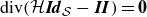 $ {\operatorname {div}}(\mathcal{H}{\boldsymbol{I\!d}}_{\mathcal{S}} - \boldsymbol{I\!I}) = \boldsymbol{0}$
, we obtain
$ {\operatorname {div}}(\mathcal{H}{\boldsymbol{I\!d}}_{\mathcal{S}} - \boldsymbol{I\!I}) = \boldsymbol{0}$
, we obtain
 \begin{align} \boldsymbol{\sigma }_{\bar {\kappa }} = \boldsymbol{0}, \qquad \boldsymbol{\eta }_{\bar {\kappa }} = \frac {9}{2}\bar {\kappa } \beta \left ( \mathcal{H}{\boldsymbol{I\!d}}_{\mathcal{S}} - \boldsymbol{I\!I} \right ) \boldsymbol{\nabla }\!\beta \end{align}
for the associated stress. Forces are given by
 \begin{align} \begin{aligned} \omega _{\bar {\kappa }} &= \frac {2}{3}(\partial _\beta u_{\bar {\kappa }}) \mathcal{K} = 3\bar {\kappa } \mathcal{K} \beta ,\\ \boldsymbol{f}_{\bar {\kappa }} &= -\boldsymbol{I\!I}\boldsymbol{\eta }_{\bar {\kappa }} = -\frac {9}{2}\bar {\kappa } \mathcal{K} \beta \boldsymbol{\nabla }\!\beta = -\frac {3}{2}\omega _{\bar {\kappa }} \boldsymbol{\nabla }\!\beta , \\ f^{\bot }_{\bar {\kappa }} &= \operatorname {div}\boldsymbol{\eta }_{\bar {\kappa }} = -\frac {9}{2} \bar {\kappa } \left ( \beta \boldsymbol{I\!I}\operatorname {:}\boldsymbol{\nabla} ^2 \beta - \mathcal{H}\beta \Delta \beta + (\boldsymbol{\nabla }\!\beta )\boldsymbol{I\!I}\boldsymbol{\nabla }\!\beta - \mathcal{H} {\left \| \boldsymbol{\nabla }\!\beta \right \|}_{{T}\! {\mathcal{S}}}^2\right ) \!, \end{aligned} \end{align}
where we used the fact that
 $ \boldsymbol{I\!I}^2 = \mathcal{H}\boldsymbol{I\!I} - \mathcal{K}{\boldsymbol{I\!d}}_{\mathcal{S}}$
is valid.
$ \boldsymbol{I\!I}^2 = \mathcal{H}\boldsymbol{I\!I} - \mathcal{K}{\boldsymbol{I\!d}}_{\mathcal{S}}$
is valid.
For the double-well potential
 $ \mathfrak{U}_{\text{d}w} := \int _{\mathcal{S}} u_{\text{d}w} {\text {d}\mathcal{S}}$
, we can once more employ Bachini et al. (Reference Bachini, Krause, Nitschke and Voigt2023a
) and obtain
$ \mathfrak{U}_{\text{d}w} := \int _{\mathcal{S}} u_{\text{d}w} {\text {d}\mathcal{S}}$
, we can once more employ Bachini et al. (Reference Bachini, Krause, Nitschke and Voigt2023a
) and obtain
 \begin{align} \begin{aligned} u_{\text{d}w} &= \frac {9}{4}\beta ^2\left ( \frac {\hat {a}}{9}\left ( \frac {2}{3}-\beta \right )^2 - \frac {3\varpi }{2}\beta \left ( 4-\frac {9}{2}\beta \right ) \right )\! , &\boldsymbol{\sigma }_{\text{d}w} &= u_{\text{d}w}{\boldsymbol{I\!d}}_{\mathcal{S}} ,\\ \omega _{\text{d}w} &= -\frac {2}{3}\partial _\beta u_{\text{d}w} = -\frac {1}{6}\beta \left ( \frac {2}{3} - \beta \right )\left ( 4 \hat {a}\left ( \frac {1}{3}-\beta \right )-243\varpi \beta \right )\! , &\boldsymbol{\eta }_{\text{d}w} &= \boldsymbol{0}, \\ \boldsymbol{f}_{\text{d}w} &= \boldsymbol{\nabla }u_{\text{d}w} = -\frac {3}{2}\omega _{\text{d}w}\boldsymbol{\nabla }\!\beta , &f^{\bot }_{\text{d}w} &= \mathcal{H} u_{\text{d}w}. \end{aligned} \end{align}
It should be noted that the fluid force
 $ \boldsymbol{F}_{\text{d}w}=\boldsymbol{f}_{\text{d}w} + f^{\bot }_{\text{d}w}\boldsymbol{\nu }$
is not an applied force in inextensible materials and could be neglected, since
$ \boldsymbol{F}_{\text{d}w}=\boldsymbol{f}_{\text{d}w} + f^{\bot }_{\text{d}w}\boldsymbol{\nu }$
is not an applied force in inextensible materials and could be neglected, since
 $ \boldsymbol{F}_{\text{d}w} = {\operatorname {Grad}}_{\textsf{C}} u_{\text{d}w}$
is a pure pressure force.
$ \boldsymbol{F}_{\text{d}w} = {\operatorname {Grad}}_{\textsf{C}} u_{\text{d}w}$
is a pure pressure force.
B.3. Flux potentials
As demonstrated in § 4.2, the lipid ansatz (4.1) can be used without considering additional lipid constraint forces. Consequently, the flux forces and stresses of the surface-conforming model in Appendix D may also be evaluated with
 $ \boldsymbol{q}=\boldsymbol{0}$
. However, it is useful to explicitly write down the flux potentials resulting from the ansatz (4.1) for a better understanding, and to employ the corresponding variations as an additional means of verification, since ‘Variation
$ \boldsymbol{q}=\boldsymbol{0}$
. However, it is useful to explicitly write down the flux potentials resulting from the ansatz (4.1) for a better understanding, and to employ the corresponding variations as an additional means of verification, since ‘Variation
 $ \circ$
Restriction’ is commutative in the absence of constraints forces. Nevertheless, we will keep the following calculations brief.
$ \circ$
Restriction’ is commutative in the absence of constraints forces. Nevertheless, we will keep the following calculations brief.
By the lipid ansatz (4.1) the anisotropic fluid metric yields
 \begin{align} {\boldsymbol{I}}_{\xi }[\beta ] &:= {\boldsymbol{I}}_{\xi }[\boldsymbol{Q}] = {\boldsymbol{I\!d}} - \xi \boldsymbol{Q} = \left (1+\frac {\xi }{2}\beta \right ){\boldsymbol{I\!d}}_{\mathcal{S}} + \left ( 1-\xi \beta \right )\boldsymbol{\nu }\otimes \boldsymbol{\nu }, \end{align}
where
 $ \xi \in {\mathbb{R}}$
is the anisotropy coefficient. Its temporal distortion is given by the lower-convected rate (Nitschke & Voigt Reference Nitschke and Voigt2023)
$ \xi \in {\mathbb{R}}$
is the anisotropy coefficient. Its temporal distortion is given by the lower-convected rate (Nitschke & Voigt Reference Nitschke and Voigt2023)
 \begin{align} \operatorname {D}^{\flat }_t{\boldsymbol{I}}_{\xi }[\beta ] &= \left (1+\frac {\xi }{2}\beta \right ){\boldsymbol{I\!d}}_{\mathcal{S}}\left ( \boldsymbol{\nabla} _{\!\textsf{C}}\boldsymbol{V} + \boldsymbol{\nabla} _{\!\textsf{C}}^T\boldsymbol{V} \right ){\boldsymbol{I\!d}}_{\mathcal{S}} -\xi \dot {\beta } \left ( \boldsymbol{\nu }\otimes \boldsymbol{\nu } - \frac {1}{2}{\boldsymbol{I\!d}}_{\mathcal{S}} \right ) \end{align}
and determine the heat released by material deformations modulo rigid-body motions. The associated viscous flux potential
 $ \mathfrak{R}_{\textit{NV}} = ({\upsilon }/{4}) \| \operatorname {D}^{\flat }_t{\boldsymbol{I}}_{\xi }[\beta ] \|_{\textrm{L}^2({T}^2\mathbb{R}^3\vert _{\mathcal{S}})}^2$
reads
$ \mathfrak{R}_{\textit{NV}} = ({\upsilon }/{4}) \| \operatorname {D}^{\flat }_t{\boldsymbol{I}}_{\xi }[\beta ] \|_{\textrm{L}^2({T}^2\mathbb{R}^3\vert _{\mathcal{S}})}^2$
reads
 \begin{align} \mathfrak{R}_{\textit{NV}} &= \frac {\upsilon }{8} \Bigg ( 2 \left \| \left (1+\frac {\xi }{2} \beta \right ) \boldsymbol{I\!d}_{\mathcal{S}}\left ( \boldsymbol{\nabla} _{\!\textsf{C}}\boldsymbol{V} + \boldsymbol{\nabla} _{\!\textsf{C}}^T\boldsymbol{V} \right ){\boldsymbol{I\!d}}_{\mathcal{S}}\right \|^2_{\textrm{L}^2({T}^2\mathcal{S})}\\ &\quad + 3 \xi ^2 \left \| \dot {\beta }\right \|^2_{\textrm{L}^2({T}^2\mathcal{S})} + 4 \xi \left \langle {\left (1+\frac {\xi }{2}\beta \right )\dot {\beta }, {\operatorname {Div}}_{\textsf{C}}\boldsymbol{V}}\right \rangle \Bigg )^2_{\textrm{L}^2({T}^2\mathcal{S})} ,\nonumber \end{align}
where
 $ \upsilon \ge 0$
is the isotropic viscosity. Variation with respect to process variables
$ \upsilon \ge 0$
is the isotropic viscosity. Variation with respect to process variables
 $ \dot {\beta }$
and
$ \dot {\beta }$
and
 $ \boldsymbol{V}=\boldsymbol{v} + v_{\bot }\boldsymbol{\nu }$
yields
$ \boldsymbol{V}=\boldsymbol{v} + v_{\bot }\boldsymbol{\nu }$
yields
 \begin{align} \begin{aligned} \omega _{\text {NV}} &= - \xi \upsilon \left ( \frac {\xi }{2} \dot {\beta } + \frac {1}{3}\left (1+\frac {\xi }{2}\beta \right )\left ( {\operatorname {div}}\boldsymbol{v} - \mathcal{H}v_{\bot } \right ) \right )\! ,\\ \boldsymbol{\sigma }_{\textit{NV}} &= \upsilon \left ( \left (1+\frac {\xi }{2}\beta \right )^2\left ( \boldsymbol{\nabla }\boldsymbol{v} + \boldsymbol{\nabla} ^T\boldsymbol{v} - 2v_{\bot }\boldsymbol{I\!I} \right ) + \frac {\xi }{2}\dot {\beta }\left (1+\frac {\xi }{2}\beta \right ){\boldsymbol{I\!d}}_{\mathcal{S}}\right )\!, &\boldsymbol{\eta }_{\textit{NV}} &= \boldsymbol{0}, \end{aligned} \end{align}
which equals the viscosity contributions in the surface-conforming model in Appendix D, respectively Nitschke & Voigt (Reference Nitschke and Voigt2025b
), for
 $ \boldsymbol{q}=\boldsymbol{0}$
. It should be noted that, in inextensible materials, the trailing summands can be neglected since they either vanish or lead to a pressure gradient. Note that, for comparisons with table 5, it holds that
$ \boldsymbol{q}=\boldsymbol{0}$
. It should be noted that, in inextensible materials, the trailing summands can be neglected since they either vanish or lead to a pressure gradient. Note that, for comparisons with table 5, it holds that
 $ \omega _{\textit{NV}} = \xi ^2(\tilde {\omega }^2_{\textit{NV}} - {\upsilon }\dot {\beta }/{2})$
and
$ \omega _{\textit{NV}} = \xi ^2(\tilde {\omega }^2_{\textit{NV}} - {\upsilon }\dot {\beta }/{2})$
and
 $ \boldsymbol{\sigma }_{\textit{NV}} = \boldsymbol{\sigma }_{\textit{NV}}^0 + \xi \boldsymbol{\sigma }_{\textit{NV}}^1 + \xi ^2\boldsymbol{\sigma }_{\textit{NV}}^2$
. Although we would not recommend proceeding in this way, for completeness, the tangential and normal fluid forces for isotropic viscous fluids (
$ \boldsymbol{\sigma }_{\textit{NV}} = \boldsymbol{\sigma }_{\textit{NV}}^0 + \xi \boldsymbol{\sigma }_{\textit{NV}}^1 + \xi ^2\boldsymbol{\sigma }_{\textit{NV}}^2$
. Although we would not recommend proceeding in this way, for completeness, the tangential and normal fluid forces for isotropic viscous fluids (
 $\xi =0$
) are
$\xi =0$
) are
 \begin{align} \boldsymbol{f}_{\textit{iso}} &:=\upsilon {\operatorname {div}}\left ( \boldsymbol{\nabla }\boldsymbol{v} + \boldsymbol{\nabla} ^T\boldsymbol{v} - 2v_{\bot }\boldsymbol{I\!I} \right ) \nonumber\\ & = \upsilon \left (\Delta \boldsymbol{v} + \mathcal{K}\boldsymbol{v} - 2\left ( \boldsymbol{I\!I} - \frac {\mathcal{H}}{2}{\boldsymbol{I\!d}}_{\mathcal{S}} \right )\boldsymbol{\nabla }v_{\bot } - v_{\bot }\boldsymbol{\nabla }\mathcal{H} + \boldsymbol{\nabla }\left ( {\operatorname {div}}\boldsymbol{v} - v_{\bot }\mathcal{H} \right )\right )\! ,\nonumber \\ f^{\bot }_{\textit{iso}} &:= \upsilon \boldsymbol{I\!I}\operatorname {:}\left ( \boldsymbol{\nabla }\boldsymbol{v} + \boldsymbol{\nabla} ^T\boldsymbol{v} - 2v_{\bot }\boldsymbol{I\!I} \right ) = 2\upsilon \left ( \boldsymbol{I\!I}\operatorname {:}\boldsymbol{\nabla }\boldsymbol{v} - v_{\bot }\left ( \mathcal{H}^2 - \mathcal{K} \right ) \right )\!, \end{align}
see Arroyo & DeSimone (Reference Arroyo and DeSimone2009), Reuther et al. (Reference Reuther, Nitschke and Voigt2020), and yield the more general forces
 \begin{align} \begin{aligned} \boldsymbol{f}_{\textit{NV}} &= \left (1+\frac {\xi }{2}\beta \right )^2 \boldsymbol{f}_{\textit{iso}} \\ & +\upsilon \left (\xi \left (1+\frac {\xi }{2}\beta \right )\left ( \boldsymbol{\nabla }\boldsymbol{v} + \boldsymbol{\nabla} ^T\boldsymbol{v} - 2v_{\bot }\boldsymbol{I\!I} \right )\boldsymbol{\nabla }\!\beta +\frac {\xi ^2}{4}\dot {\beta }\boldsymbol{\nabla }\!\beta + \frac {\xi }{2}\left (1+\frac {\xi }{2}\beta \right )\boldsymbol{\nabla }\dot {\beta } \right )\!, \\ f^{\bot }_{\textit{NV}} &= \left (1+\frac {\xi }{2}\beta \right )^2f^{\bot }_{\textit{iso}} +\frac {\xi \upsilon }{2}\dot {\beta }\left (1+\frac {\xi }{2}\beta \right )\mathcal{H} . \end{aligned} \end{align}
Next, we address the immobility flux potential
 $ \mathfrak{R}_{{IM}}^{\varPhi }=\frac {M}{2} \left \| \mathrm{D}^{\varPhi }_t \boldsymbol{Q} \right \|^2_{{\textrm{L}}^2({T}^2\mathbb{R}\vert _{\textrm{S}})}$
with
$ \mathfrak{R}_{{IM}}^{\varPhi }=\frac {M}{2} \left \| \mathrm{D}^{\varPhi }_t \boldsymbol{Q} \right \|^2_{{\textrm{L}}^2({T}^2\mathbb{R}\vert _{\textrm{S}})}$
with
 $ \varPhi \in \{\mathfrak{m},\mathcal{J}\}$
, where
$ \varPhi \in \{\mathfrak{m},\mathcal{J}\}$
, where
 \begin{align} \operatorname {D}^{\mathfrak{m}}_t\boldsymbol{Q} &= \dot {\beta }\left ( \boldsymbol{\nu }\otimes \boldsymbol{\nu } - \frac {1}{2}{\boldsymbol{I\!d}}_{\mathcal{S}} \right ) -\frac {3}{2}\beta \left ( \boldsymbol{\nu }\boldsymbol{\nabla} _{\!\textsf{C}}\boldsymbol{V} \otimes \boldsymbol{\nu } + \boldsymbol{\nu } \otimes \boldsymbol{\nu }\boldsymbol{\nabla} _{\!\textsf{C}}\boldsymbol{V} \right )\! , \nonumber \\ \operatorname {D}^{\mathcal{J}}_t\boldsymbol{Q} &= \dot {\beta }\left ( \boldsymbol{\nu }\otimes \boldsymbol{\nu } - \frac {1}{2}{\boldsymbol{I\!d}}_{\mathcal{S}} \right ) \end{align}
holds by Nitschke & Voigt (Reference Nitschke and Voigt2023) and lipid ansatz (4.1). This results in
 \begin{align} \mathfrak{R}_{\textit{IM}}^{\mathfrak{m}} &= \frac {3 M}{4}\left ( \left \| \dot {\beta } \right \|_{{L}^2 ({T}^0\mathcal{S})}^2+ 3 \left \| \beta {\nu } \boldsymbol{\nabla} _{\!\textsf{C}}\boldsymbol{V}\right \|_{\textrm{L}^2 ({T} \mathcal{S})}^2\right )\! , &\mathfrak{R}_{\textit{IM}}^{\mathcal{J}} &= \frac {3 M}{4} \left \| \dot {\beta } \right \|_{\textrm{L}^2 ({T}^0 \mathcal{S})}^2. \end{align}
Variation with respect to process variables
 $ \dot {\beta }$
and
$ \dot {\beta }$
and
 $ \boldsymbol{V}=\boldsymbol{v} + v_{\bot }\boldsymbol{\nu }$
yields
$ \boldsymbol{V}=\boldsymbol{v} + v_{\bot }\boldsymbol{\nu }$
yields
 \begin{align} \begin{aligned} \omega _{\textit{IM}}^{\mathfrak{m}} &= \omega _{\textit{IM}}^{\mathcal{J}} = -M \dot {\beta }, \\ \boldsymbol{\sigma }_{\textit{IM}}^{\mathfrak{m}} &= \boldsymbol{\sigma }_{\textit{IM}}^{\mathcal{J}} = \boldsymbol{0}, &\boldsymbol{\eta }_{\textit{IM}}^{\mathfrak{m}} &= \frac {9 M}{2} \beta ^2\left ( \boldsymbol{\nabla }v_{\bot } + \boldsymbol{I\!I}\boldsymbol{v} \right )\!, &\boldsymbol{\eta }_{\textit{IM}}^{\mathcal{J}} &= \boldsymbol{0} . \end{aligned} \end{align}
This also agrees with the surface-conforming model in Appendix D, respectively Nitschke & Voigt (Reference Nitschke and Voigt2025b
), for
 $ \boldsymbol{q}=\boldsymbol{0}$
. It should be noted that the surface-conforming model does not impose any normal immobility stresses
$ \boldsymbol{q}=\boldsymbol{0}$
. It should be noted that the surface-conforming model does not impose any normal immobility stresses
 $ \boldsymbol{\eta }_{\textit{IM}}^{\varPhi }$
directly. Instead, it comprises constraint forces to ensure surface conformity, e.g. in terms of
$ \boldsymbol{\eta }_{\textit{IM}}^{\varPhi }$
directly. Instead, it comprises constraint forces to ensure surface conformity, e.g. in terms of
 $ \boldsymbol{\zeta }_{\textit{IM}}^{\varPhi }{{T}\! {\mathcal{S}}}$
. However, the lipid ansatz (4.1) already stipulates surface conformity a priori. Both procedures are equivalent eventually and, for
$ \boldsymbol{\zeta }_{\textit{IM}}^{\varPhi }{{T}\! {\mathcal{S}}}$
. However, the lipid ansatz (4.1) already stipulates surface conformity a priori. Both procedures are equivalent eventually and, for
 $ \boldsymbol{q} = \boldsymbol{0}$
, it holds that
$ \boldsymbol{q} = \boldsymbol{0}$
, it holds that
 $ \boldsymbol{\eta }_{\textit{IM}}^{\varPhi } = 3\beta \boldsymbol{\zeta }_{\textit{IM}}^{\varPhi }$
and, thus, gives the same immobility force in the fluid equation. For the sake of completeness, the resulting fluid forces in tangential and normal directions are
$ \boldsymbol{\eta }_{\textit{IM}}^{\varPhi } = 3\beta \boldsymbol{\zeta }_{\textit{IM}}^{\varPhi }$
and, thus, gives the same immobility force in the fluid equation. For the sake of completeness, the resulting fluid forces in tangential and normal directions are
 \begin{align} \begin{aligned} \boldsymbol{f}_{\textit{IM}}^{\mathfrak{m}} &= \frac {9 M}{2} \beta ^2\left ( \mathcal{K}\boldsymbol{v} - \boldsymbol{I\!I}\left ( \boldsymbol{\nabla }v_{\bot } + \mathcal{H}\boldsymbol{v} \right ) \right )\!, &\boldsymbol{f}_{\textit{IM}}^{\mathcal{J}} &= \boldsymbol{0}, \\ f^{\mathfrak{m},\bot }_{\textit{IM}} &= \frac {9 M}{2} \beta \left ( \left ( \Delta v_{\bot } + \boldsymbol{I\!I}\operatorname {:}\boldsymbol{\nabla }\boldsymbol{v} + \boldsymbol{\nabla} _{\boldsymbol{v}}\mathcal{H} \right )\beta + 2\left ( \boldsymbol{\nabla }v_{\bot } + \boldsymbol{v}\boldsymbol{I\!I} \right )\boldsymbol{\nabla }\!\beta \right ) , &f^{\mathcal{J},\bot }_{\textit{IM}} &= 0 . \end{aligned} \end{align}
The activity flux potential
 $ \mathfrak{R}_{{{AC}}} = ({\alpha }/{2})\int _{\mathcal{S}}({\operatorname {Tr}}\circ \operatorname {D}^{\flat }_t{\boldsymbol{I}}_{\xi }[\boldsymbol{Q}]){\text {d}\mathcal{S}}$
, which stated the first moment of the temporal anisotropic metric distortion, is not relevant for lipids on an inextensible medium. This can be seen by (B13), which yields
$ \mathfrak{R}_{{{AC}}} = ({\alpha }/{2})\int _{\mathcal{S}}({\operatorname {Tr}}\circ \operatorname {D}^{\flat }_t{\boldsymbol{I}}_{\xi }[\boldsymbol{Q}]){\text {d}\mathcal{S}}$
, which stated the first moment of the temporal anisotropic metric distortion, is not relevant for lipids on an inextensible medium. This can be seen by (B13), which yields
 \begin{align} \mathfrak{R}_{{{AC}}} = \alpha \int _{\mathcal{S}} \left ( 1 + \frac {\xi }{2}\beta \right ) {\operatorname {Div}}_{\textsf{C}}\boldsymbol{V} {\text {d}\mathcal{S}} . \end{align}
Variations result in
 \begin{align} \begin{aligned} \omega _{{{AC}}} &= 0 , &\boldsymbol{\sigma }_{\!{{AC}}} &= \alpha \left ( 1 + \frac {\xi }{2}\beta \right ) {\boldsymbol{I\!d}}_{\mathcal{S}}, & \boldsymbol{\eta }_{{{AC}}} &= \boldsymbol{0} ,\\ & &\boldsymbol{f}_{\!{{AC}}} &= \alpha \boldsymbol{\nabla }\left ( 1 + \frac {\xi }{2}\beta \right ) = \frac {\alpha \xi }{2}\boldsymbol{\nabla }\!\beta , &f^{\bot }_{{AC}} &= \alpha \left ( 1 + \frac {\xi }{2}\beta \right )\mathcal{H}. \end{aligned} \end{align}
This means we only get an active pressure term, which has not any influence of the solution for an inextensible fluid and, thus, can be neglected. Although it is irrelevant for the present paper, it should be noted that
 $ \boldsymbol{\sigma }_{\!{{AC}}}$
gives rise to geometric activity (Nitschke & Voigt Reference Nitschke and Voigt2025a
) or active tension (Mietke et al. Reference Mietke, Jemseena, Kumar, Sbalzarini and Jülicher2019; Wittwer & Aland Reference Wittwer and Aland2023), respectively contributes to the membrane tension (Al-Izzi & Alexander Reference Al-Izzi and Alexander2023), depending on the scalar order in an extensible medium.
$ \boldsymbol{\sigma }_{\!{{AC}}}$
gives rise to geometric activity (Nitschke & Voigt Reference Nitschke and Voigt2025a
) or active tension (Mietke et al. Reference Mietke, Jemseena, Kumar, Sbalzarini and Jülicher2019; Wittwer & Aland Reference Wittwer and Aland2023), respectively contributes to the membrane tension (Al-Izzi & Alexander Reference Al-Izzi and Alexander2023), depending on the scalar order in an extensible medium.
Appendix C. Energy rate
In this section we discuss the energy rate
 $({{\textrm d}}/{{\textrm d}t}){\mathfrak{E}}_{\textit{TOT}}$
of the total energy
$({{\textrm d}}/{{\textrm d}t}){\mathfrak{E}}_{\textit{TOT}}$
of the total energy
 \begin{align} \mathfrak{E}_{\textit{TOT}} &:= \int _{\mathcal{S}} \frac {\rho }{2} \left \| \boldsymbol{V} \right \|_{{T}{{\mathbb{R}}^3\vert _{\mathcal{S}}} }^2{{\textrm d}\mathcal{S}} + \mathfrak{U}_{{LH}}, \end{align}
consisting of the kinetic energy and the potential energy, the latter being given solely by the LH energy (4.25). Conceptually, one may either appeal to the intermediate result in Nitschke & Voigt (Reference Nitschke and Voigt2025b ) for the energy rate under the ansatz (4.1) or one may rederive it following the same procedure as in Nitschke & Voigt (Reference Nitschke and Voigt2025b ) within our framework. Either way, the Lagrange–d’Alembert principle yields the physical power balance
 \begin{align} \frac {\text {d} }{\text {d} \mathfrak{E}}{t}_{\textit{TOT}} &= \mathfrak{P}_{\textit{TOT}} = \mathfrak{P}_{\textit{NV}} + \mathfrak{P}_{\textit{IM}}^{\varPhi } + \mathfrak{P}_{{{AC}}} \end{align}
for solutions of the governing equations (3.4), where the individual power inputs
 $ \mathfrak{P}_{\bullet }$
due to anisotropic viscosity, immobility and activity fluxes are given by the product of generalised forces
$ \mathfrak{P}_{\bullet }$
due to anisotropic viscosity, immobility and activity fluxes are given by the product of generalised forces
 $ (\boldsymbol{F}_{\bullet }, {\boldsymbol{H}}_{\bullet } ) \in {T}{{\mathbb{R}}^3\vert _{\mathcal{S}}}\times {\operatorname {\mathcal{Q}}}{^2}{\mathbb{R}}^3\vert _{\mathcal{S}}$
, respectively
$ (\boldsymbol{F}_{\bullet }, {\boldsymbol{H}}_{\bullet } ) \in {T}{{\mathbb{R}}^3\vert _{\mathcal{S}}}\times {\operatorname {\mathcal{Q}}}{^2}{\mathbb{R}}^3\vert _{\mathcal{S}}$
, respectively
 $ ( \boldsymbol{f}_{\bullet }, f^{\bot }_{\bullet }, \omega _{\bullet } )\in {{T}\! {\mathcal{S}}}\times {{T}^0 \mathcal{S}}\times {{T}^0 \mathcal{S}}$
, and generalised velocities
$ ( \boldsymbol{f}_{\bullet }, f^{\bot }_{\bullet }, \omega _{\bullet } )\in {{T}\! {\mathcal{S}}}\times {{T}^0 \mathcal{S}}\times {{T}^0 \mathcal{S}}$
, and generalised velocities
 $ ( \boldsymbol{V}, \operatorname {D}^{\mathfrak{m}}_t\boldsymbol{Q} ) \in {T}{{\mathbb{R}}^3\vert _{\mathcal{S}}}\times {\operatorname {\mathcal{Q}}}{^2}{\mathbb{R}}^3\vert _{\mathcal{S}}$
, respectively
$ ( \boldsymbol{V}, \operatorname {D}^{\mathfrak{m}}_t\boldsymbol{Q} ) \in {T}{{\mathbb{R}}^3\vert _{\mathcal{S}}}\times {\operatorname {\mathcal{Q}}}{^2}{\mathbb{R}}^3\vert _{\mathcal{S}}$
, respectively
 $ ( \boldsymbol{v}, v_{\bot }, \dot {\beta } )\in {{T}\! {\mathcal{S}}}\times {{T}^0 \mathcal{S}}\times {{T}^0 \mathcal{S}}$
, i.e.
$ ( \boldsymbol{v}, v_{\bot }, \dot {\beta } )\in {{T}\! {\mathcal{S}}}\times {{T}^0 \mathcal{S}}\times {{T}^0 \mathcal{S}}$
, i.e.
 \begin{align} \mathfrak{P}_{\bullet } &= \left \langle {\boldsymbol{F}_{\bullet }, \boldsymbol{V}} \right \rangle _{\textrm{L}^2({T}\mathbb{R}\vert _{\mathcal{S}})} + \left \langle {{\boldsymbol{H}}_{\bullet }, \operatorname {D}^{\mathfrak{m}}_t\boldsymbol{Q}} \right \rangle _{\textrm{L}^2(\mathcal{Q}^2\mathbb{R}^3\vert _{\mathcal{S}})} = \left \langle {\boldsymbol{f}_{\bullet }, \boldsymbol{v}} \right \rangle _{\textrm{L}^2({T}\mathcal{S})} + \big \langle {f^{\bot }_{\bullet }, v_{\bot }} \big \rangle _{\textrm{L}^2({T}^0\mathcal{S})} \nonumber \\ &\quad + \frac {3}{2}\big \langle {\omega _{\bullet }, \dot {\beta }} \big \rangle _{\textrm{L}^2({T}^0\mathcal{S})} \nonumber \\ &= -\left ( \left \langle {\boldsymbol{\sigma }_{\bullet }, \boldsymbol{\nabla }\boldsymbol{v} - v_{\bot }\boldsymbol{I\!I}} \right \rangle _{\textrm{L}^2({T}^2\mathcal{S})} +\left \langle {\boldsymbol{\eta }_{\bullet }, \boldsymbol{\nabla }v_{\bot } + \boldsymbol{I\!I}\boldsymbol{v}} \right \rangle _{\textrm{L}^2({T}\mathcal{S})} - \frac {3}{2}\big \langle {\omega _{\bullet }, \dot {\beta }} \big \rangle _{\textrm{L}^2({T}^0\mathcal{S})} \right ) \end{align}
with fluid stress fields
 $ ( \boldsymbol{\sigma }_{\bullet }, \boldsymbol{\eta }_{\bullet } )\in {{T}^2 \mathcal{S}}\times {{T}\! {\mathcal{S}}}$
(B2). Inextensibility (3.4c
) and stress/force (B15) result in
$ ( \boldsymbol{\sigma }_{\bullet }, \boldsymbol{\eta }_{\bullet } )\in {{T}^2 \mathcal{S}}\times {{T}\! {\mathcal{S}}}$
(B2). Inextensibility (3.4c
) and stress/force (B15) result in
 $ \mathfrak{P}_{\textit{NV}} = -2\mathfrak{R}_{\textit{NV}}$
(B14); stress/force (B20) yields
$ \mathfrak{P}_{\textit{NV}} = -2\mathfrak{R}_{\textit{NV}}$
(B14); stress/force (B20) yields
 $ \mathfrak{P}_{\textit{IM}}^{\varPhi } = -2 \mathfrak{R}_{\textit{IM}}^{\varPhi }$
(B19) for
$ \mathfrak{P}_{\textit{IM}}^{\varPhi } = -2 \mathfrak{R}_{\textit{IM}}^{\varPhi }$
(B19) for
 $ \varPhi \in \{\mathfrak{m}, \mathcal{J}\}$
; the activity power/flux potential
$ \varPhi \in \{\mathfrak{m}, \mathcal{J}\}$
; the activity power/flux potential
 $ \mathfrak{P}_{{{AC}}}= \mathfrak{R}_{{{AC}}} = 0$
vanishes as expected by (B23). Eventually, we summarise that
$ \mathfrak{P}_{{{AC}}}= \mathfrak{R}_{{{AC}}} = 0$
vanishes as expected by (B23). Eventually, we summarise that
 \begin{align} \frac {\text {d}}{\text {d}t} {\mathfrak{E}}_{\textit{TOT}} &= - \frac {1}{4}\left ( 2\upsilon \left \| \left (1+\frac {\xi }{2}\beta \right )\boldsymbol{I\!d}_{\mathcal{S}}\left (\boldsymbol{\nabla} _{\!\textsf{C}}\boldsymbol{V}+\boldsymbol{\nabla} ^T_{\textsf{C}}\boldsymbol{V}\right )\boldsymbol{I\!d}_{\mathcal{S}}\right \|^2_{\textrm{L}^2({T}^2\mathcal{S})}\right .\nonumber \\ &\left .\hspace {1em}+ 3 \left ( 2M + \upsilon \xi ^2\right ) \left \| \dot {\beta }\right \|_{\textrm{L}^2({T}^0 \mathcal{S})}^2{}{ } + 18M \delta _{\mathfrak{m}}^{\phi } \left \| \beta \nu \boldsymbol{\nabla} _{\!\textsf{C}}\boldsymbol{V}\right \|_{\textrm{L}^2({T} \mathcal{S})}^2\right ) \nonumber \\ &= -2 \left ( \mathfrak{R}_{\textit{NV}} + \mathfrak{R}_{\textit{IM}}^{\varPhi } \right ) \le 0 \end{align}
for solutions of the LH model (3.4). Consequently, the evolution of both the surface
 ${\mathcal{S}}$
and the scalar order parameter
${\mathcal{S}}$
and the scalar order parameter
 $ \beta$
is of a purely dissipative nature. This dissipation is irreversible and, hence, directly proportional to the entropy production.
$ \beta$
is of a purely dissipative nature. This dissipation is irreversible and, hence, directly proportional to the entropy production.
Appendix D. Surface-conforming Beris–Edwards model
In the following we merely recall the surface-conforming active Beris–Edwards model from Nitschke & Voigt (Reference Nitschke and Voigt2025a ). The full derivation and all mathematical background that is not reiterated here are provided in Nitschke & Voigt (Reference Nitschke and Voigt2025a , Reference Nitschke and Voigtb ).
Find the tangential and normal material velocity fields
 $ \boldsymbol{v}\in {{T}\! {\mathcal{S}}}$
and
$ \boldsymbol{v}\in {{T}\! {\mathcal{S}}}$
and
 $ v_{\bot }\in {{T}^0 \mathcal{S}}$
, tangential Q-tensor field
$ v_{\bot }\in {{T}^0 \mathcal{S}}$
, tangential Q-tensor field
 $ \boldsymbol{q}\in {\operatorname {\mathcal{Q}}}{^2}\mathcal{S}$
, normal eigenvalue field
$ \boldsymbol{q}\in {\operatorname {\mathcal{Q}}}{^2}\mathcal{S}$
, normal eigenvalue field
 $ \beta \in {{T}^0 \mathcal{S}}$
, pressure field
$ \beta \in {{T}^0 \mathcal{S}}$
, pressure field
 $ p\in {{T}^0 \mathcal{S}}$
and Lagrange parameter fields
$ p\in {{T}^0 \mathcal{S}}$
and Lagrange parameter fields
 $ \boldsymbol{\lambda }_{\gamma }\in \mathcal{V}_{\gamma }\le {T}^n {{\mathbb{R}}^3\vert _{\mathcal{S}}}$
for all
$ \boldsymbol{\lambda }_{\gamma }\in \mathcal{V}_{\gamma }\le {T}^n {{\mathbb{R}}^3\vert _{\mathcal{S}}}$
for all
 $ \gamma \in \mathcal{C}_{{{SC}}}$
such that
$ \gamma \in \mathcal{C}_{{{SC}}}$
such that
 \begin{align} \rho {\boldsymbol{a}} &= \boldsymbol{\nabla }\tilde {p} + {\operatorname {div}}\left ( \boldsymbol{\sigma }_{\textit{EL}} + \boldsymbol{\sigma }_{\textit{IM}}^{\varPhi }+ \boldsymbol{\sigma }_{\textit{NV}}^0 + \xi \boldsymbol{\sigma }_{\textit{NV}}^1 + \xi ^2\boldsymbol{\sigma }_{\textit{NV}}^2 +\boldsymbol{\sigma }_{\!{{NA}}}\right ) \nonumber \\ &\quad + \left (2\boldsymbol{I\!I}\boldsymbol{q}-3\beta \boldsymbol{I\!I}\right )\left ( \boldsymbol{\zeta }_{\textit{EL}} + \boldsymbol{\zeta }_{\textit{IM}}^{\varPhi }\right ) + \sum _{\gamma \in \mathcal{C}_{{{SC}}}}\boldsymbol{f}_{\gamma }, \end{align}
 \begin{align} \rho a_{\bot } &= \tilde {p}\mathcal{H} + f^{\bot }_{{BE}} + \boldsymbol{I\!I}\operatorname {:}\left ( \boldsymbol{\sigma }_{\textit{EL}} + \boldsymbol{\sigma }_{\textit{IM}}^{\varPhi } +\boldsymbol{\sigma }_{\textit{NV}}^0 + \xi \boldsymbol{\sigma }_{\textit{NV}}^1 + \xi ^2\boldsymbol{\sigma }_{\textit{NV}}^2 + \boldsymbol{\sigma }_{\!{{NA}}} \right ) \nonumber \\ &\quad - {\operatorname {div}}\left ( \left (2\boldsymbol{q}-3\beta {\boldsymbol{I\!d}}_{\mathcal{S}}\right ) \left ( \boldsymbol{\zeta }_{\textit{EL}} + \boldsymbol{\zeta }_{\textit{IM}}^{\varPhi }\right ) \right ) + \sum _{\gamma \in \mathcal{C}_{{{SC}}}} f^{\bot }_{\gamma }, \end{align}
 \begin{align} \left ( M + \frac {\upsilon \xi ^2}{2} \right )\operatorname {d}_{t}^{\varPhi }\boldsymbol{q} &= {\boldsymbol{h}}_{\textit{EL}} + {\boldsymbol{h}}_{{TH}} + \xi {\boldsymbol{h}}_{\textit{NV}}^1 + \xi ^2\widetilde {{\boldsymbol{h}}}^{2,\varPhi }_{\textit{NV}} + \sum _{\gamma \in \mathcal{C}_{{{SC}}}} {\boldsymbol{h}}_{\gamma }, \end{align}
 \begin{align} \left ( M + \frac {\upsilon \xi ^2}{2} \right ) \dot {\beta } &= \omega _{\text {EL}} + \omega _{\text {TH}} + \xi ^2\widetilde {\omega }^{2}_{\textit{NV}} + \sum _{\gamma \in \mathcal{C}_{{{SC}}}} \omega _{\gamma }, \end{align}
 \begin{align} {\operatorname {div}}\boldsymbol{v} = v_{\bot }\mathcal{H}, \end{align}
 \begin{align} \forall \gamma \in \mathcal{C}_{{{SC}}}:\quad \boldsymbol{0} = {\boldsymbol{C}}_{\gamma } \end{align}
holds for
 $ \dot {\rho }=0$
and given initial conditions for
$ \dot {\rho }=0$
and given initial conditions for
 $ \boldsymbol{v}$
,
$ \boldsymbol{v}$
,
 $ v_{\bot }$
,
$ v_{\bot }$
,
 $ \boldsymbol{q}$
,
$ \boldsymbol{q}$
,
 $ \beta$
and mass density
$ \beta$
and mass density
 $ \rho \in {{T}^0 \mathcal{S}}$
.
$ \rho \in {{T}^0 \mathcal{S}}$
.
Quantities are unpacked in table 5. The choice of
 $ \varPhi$
for
$ \varPhi$
for
 $ \boldsymbol{\sigma }_{\textit{NV}}^1$
and
$ \boldsymbol{\sigma }_{\textit{NV}}^1$
and
 $ \boldsymbol{\sigma }_{\textit{NV}}^2$
is optional. Both given representations state equal tensor fields. Here
$ \boldsymbol{\sigma }_{\textit{NV}}^2$
is optional. Both given representations state equal tensor fields. Here
 $ \mathcal{C}_{{{SC}}}$
is a set of constraints suitable for surface-conforming Q-tensor fields, which might yield additional constraint forces. In this paper we only consider the ‘no flat degeneracy’ (
$ \mathcal{C}_{{{SC}}}$
is a set of constraints suitable for surface-conforming Q-tensor fields, which might yield additional constraint forces. In this paper we only consider the ‘no flat degeneracy’ (
 $ \text {ND}$
) constraint, i.e.
$ \text {ND}$
) constraint, i.e.
 $ \mathcal{C}_{{{SC}}} = \{\text {ND}\}$
holds and
$ \mathcal{C}_{{{SC}}} = \{\text {ND}\}$
holds and
 $ \boldsymbol{f}_{\textit{ND}}, f^{\bot }_{\textit{ND}}, {\boldsymbol{h}}_{\textit{ND}}, \omega _{\text {ND}}, {\boldsymbol{C}}_{\textit{ND}}$
are the associated generalised constraint forces derived in Appendix E. Since this is an inextensible model, we summarise obvious pressure terms into the generalised pressure
$ \boldsymbol{f}_{\textit{ND}}, f^{\bot }_{\textit{ND}}, {\boldsymbol{h}}_{\textit{ND}}, \omega _{\text {ND}}, {\boldsymbol{C}}_{\textit{ND}}$
are the associated generalised constraint forces derived in Appendix E. Since this is an inextensible model, we summarise obvious pressure terms into the generalised pressure
 $ \tilde {p}\in {{T}^0 \mathcal{S}}$
for simplicity.
$ \tilde {p}\in {{T}^0 \mathcal{S}}$
for simplicity.
Appendix E. No flat degeneracy constraint
The ‘no flat degeneracy’ constraint may be given by
 \begin{align} \boldsymbol{0} &= \boldsymbol{q} = (\operatorname {\varPi }_{{\operatorname {\mathcal{Q}}}{^2}\mathcal{S}}\circ {\operatorname {\varPi }_{{{T}^2 \mathcal{S}}}})\boldsymbol{Q} = {\boldsymbol{I\!d}}_{\mathcal{S}}\boldsymbol{Q}{\boldsymbol{I\!d}}_{\mathcal{S}}-\frac {\boldsymbol{Q}\operatorname {:}{\boldsymbol{I\!d}}_{\mathcal{S}}}{2}{\boldsymbol{I\!d}}_{\mathcal{S}} = {\boldsymbol{C}}_{\textit{ND}}, \end{align}
where
 $ {\operatorname {\varPi }_{{{T}^2 \mathcal{S}}}}:{T}^2 {{\mathbb{R}}^3\vert _{\mathcal{S}}} \rightarrow {{T}^2 \mathcal{S}}$
is the orthogonal tangential projection on two-tensor fields with
$ {\operatorname {\varPi }_{{{T}^2 \mathcal{S}}}}:{T}^2 {{\mathbb{R}}^3\vert _{\mathcal{S}}} \rightarrow {{T}^2 \mathcal{S}}$
is the orthogonal tangential projection on two-tensor fields with
 $ {\operatorname {\varPi }_{{{T}^2 \mathcal{S}}}}{\boldsymbol{R}} = {\boldsymbol{I\!d}}_{\mathcal{S}}{\boldsymbol{R}}{\boldsymbol{I\!d}}_{\mathcal{S}}$
for all
$ {\operatorname {\varPi }_{{{T}^2 \mathcal{S}}}}{\boldsymbol{R}} = {\boldsymbol{I\!d}}_{\mathcal{S}}{\boldsymbol{R}}{\boldsymbol{I\!d}}_{\mathcal{S}}$
for all
 $ {\boldsymbol{R}}\in T^2 {{\mathbb{R}}^3\vert _{\mathcal{S}}}$
, and
$ {\boldsymbol{R}}\in T^2 {{\mathbb{R}}^3\vert _{\mathcal{S}}}$
, and
 $ \operatorname {\varPi }_{{\operatorname {\mathcal{Q}}}{^2}\mathcal{S}}: {{T}^2 \mathcal{S}} \rightarrow {\operatorname {\mathcal{Q}}}{^2}\mathcal{S}$
is the orthogonal flat-degenerated Q-tensor projection on tangential two-tensor fields with
$ \operatorname {\varPi }_{{\operatorname {\mathcal{Q}}}{^2}\mathcal{S}}: {{T}^2 \mathcal{S}} \rightarrow {\operatorname {\mathcal{Q}}}{^2}\mathcal{S}$
is the orthogonal flat-degenerated Q-tensor projection on tangential two-tensor fields with
 $ \operatorname {\varPi }_{{\operatorname {\mathcal{Q}}}{^2}\mathcal{S}} {\boldsymbol{r}} = ({1}/{2}) ( {\boldsymbol{r}} + {\boldsymbol{r}}^T - ({\operatorname {Tr}}{\boldsymbol{r}}){\boldsymbol{I\!d}}_{\mathcal{S}} )$
. To implement this into the surface-conforming model (D1), we introduce the Lagrange functional
$ \operatorname {\varPi }_{{\operatorname {\mathcal{Q}}}{^2}\mathcal{S}} {\boldsymbol{r}} = ({1}/{2}) ( {\boldsymbol{r}} + {\boldsymbol{r}}^T - ({\operatorname {Tr}}{\boldsymbol{r}}){\boldsymbol{I\!d}}_{\mathcal{S}} )$
. To implement this into the surface-conforming model (D1), we introduce the Lagrange functional
 \begin{align} \mathfrak{U}_{\textit{ND}} := -\left \langle \boldsymbol{\lambda }_{\textit{ND}},(\operatorname {\varPi }_{\operatorname {\mathcal{Q}}^2\mathcal{S}} \circ \operatorname {\varPi }_{{T}^2\mathcal{S}})\boldsymbol{Q}\right \rangle _{\textrm{L}^2 (\mathcal{Q}^2\mathcal{S})} = -\left \langle \boldsymbol{\lambda }_{\textit{ND}},\boldsymbol{Q} \right \rangle _{\textrm{L}^2 (\mathcal{Q}^2\mathbb{R}^3\vert _{\mathcal{S}})} \end{align}
as a potential energy, with Lagrange parameter
 $ \boldsymbol{\lambda }_{\textit{ND}}\in {\operatorname {\mathcal{Q}}}{^2}\mathcal{S}$
yielding an additional degree of freedom. The variation
$ \boldsymbol{\lambda }_{\textit{ND}}\in {\operatorname {\mathcal{Q}}}{^2}\mathcal{S}$
yielding an additional degree of freedom. The variation
 \begin{align} \left \langle {{\boldsymbol{C}}_{\textit{ND}}, \boldsymbol{\theta }} \right \rangle _{\textrm{L}^2 (\mathcal{Q}^2\mathcal{S})} &:=-\left \langle {\frac {\delta \mathfrak{U}_{\textit{ND}}}{\delta \boldsymbol{\lambda }_{\textit{ND}}}, \boldsymbol{\theta }} \right \rangle _{\textrm{L}^2 (\mathcal{Q}^2 {\mathcal{S}})} = 0 \end{align}
for all virtual displacements
 $ \boldsymbol{\theta }\in {\operatorname {\mathcal{Q}}}{^2}\mathcal{S}$
results in the constraint equation (E1). The molecular constraint force
$ \boldsymbol{\theta }\in {\operatorname {\mathcal{Q}}}{^2}\mathcal{S}$
results in the constraint equation (E1). The molecular constraint force
 ${\boldsymbol{H}}_{\textit{ND}}\in {\operatorname {\mathcal{Q}}}{^2}{\mathbb{R}}^3\vert _{\mathcal{S}}$
is given by the variation
${\boldsymbol{H}}_{\textit{ND}}\in {\operatorname {\mathcal{Q}}}{^2}{\mathbb{R}}^3\vert _{\mathcal{S}}$
is given by the variation
 \begin{align} \left \langle {{\boldsymbol{H}}_{\textit{ND}}, \boldsymbol{\varPsi }} \right \rangle _{\textrm{L}^2 (\mathcal{Q}^2\mathbb{R}^3\vert _{\mathcal{S}})} &:= -\left \langle {\frac {\delta \mathfrak{U}_{\textit{ND}}}{\delta \boldsymbol{Q}}, \boldsymbol{\varPsi }}\right \rangle _{\textrm{L}^2 (\mathcal{Q}^2\mathbb{R}^3\vert _{\mathcal{S}})} = \left \langle {\boldsymbol{\lambda }_{\textit{ND}}, \boldsymbol{\varPsi }} \right \rangle _{\textrm{L}^2 (\mathcal{Q}^2\mathbb{R}^3\vert _{\mathcal{S}})} \end{align}
for all virtual displacements
 $ \boldsymbol{\varPsi }\in {\operatorname {\mathcal{Q}}}{^2}{\mathbb{R}}^3\vert _{\mathcal{S}}$
. Therefore, the constraint force is flat degenerated and we have to add
$ \boldsymbol{\varPsi }\in {\operatorname {\mathcal{Q}}}{^2}{\mathbb{R}}^3\vert _{\mathcal{S}}$
. Therefore, the constraint force is flat degenerated and we have to add
 \begin{align} {\boldsymbol{h}}_{\textit{ND}} := (\operatorname {\varPi }_{{\operatorname {\mathcal{Q}}}{^2}\mathcal{S}}\circ {\operatorname {\varPi }_{{{T}^2 \mathcal{S}}}}){\boldsymbol{H}}_{\textit{ND}} = {\boldsymbol{H}}_{\textit{ND}} = \boldsymbol{\lambda }_{\textit{ND}} \in {{\mathcal{Q}}}^2\mathcal{S} \end{align}
to the right-hand side of the flat-degenerated molecular equation (D1c). Since
 $\boldsymbol{\lambda }_{\textit{ND}}$
is fully determined by that equation, we can, in principle, omit it. However, as is the case with the surface-conforming constraint in Nitschke & Voigt (Reference Nitschke and Voigt2025b
), an additional constraint force
$\boldsymbol{\lambda }_{\textit{ND}}$
is fully determined by that equation, we can, in principle, omit it. However, as is the case with the surface-conforming constraint in Nitschke & Voigt (Reference Nitschke and Voigt2025b
), an additional constraint force
 $ \boldsymbol{F}_{\textit{ND}} = \boldsymbol{f}_{\textit{ND}} + f^{\bot }_{\textit{ND}}\boldsymbol{\nu }$
may need to be accounted for in the fluid equations (D1a
) and (D1b
). Spatial state variation yields
$ \boldsymbol{F}_{\textit{ND}} = \boldsymbol{f}_{\textit{ND}} + f^{\bot }_{\textit{ND}}\boldsymbol{\nu }$
may need to be accounted for in the fluid equations (D1a
) and (D1b
). Spatial state variation yields
 \begin{align} & \left \langle {\boldsymbol{F}_{\textit{ND}}, \boldsymbol{W}} \right \rangle _{\textrm{L}^2 ({T}\mathbb{R}^3\vert _{\mathcal{S}})} := -\left \langle {\frac {\delta \mathfrak{U}_{\textit{ND}}}{\delta \boldsymbol{X}}, \boldsymbol{W}} \right \rangle _{\textrm{L}^2 ({T}\mathbb{R}^3\vert _{\mathcal{S}})} \nonumber \\ & = \int _{\mathcal{S}} \eth _{\boldsymbol{W}}\left \langle \boldsymbol{\lambda }_{\textit{ND}},\boldsymbol{q} \right \rangle _{ {\operatorname {\mathcal{Q}}}{^2}\mathcal{S}} + \left \langle \boldsymbol{\lambda }_{\textit{ND}},\boldsymbol{q} \right \rangle _{ {\operatorname {\mathcal{Q}}}{^2}\mathcal{S}}({\operatorname {Div}}_{\textsf{C}}\boldsymbol{W}) {\text {d}\mathcal{S}}\nonumber \\ &= \left \langle {\eth _{\boldsymbol{W}}\boldsymbol{\lambda }_{\textit{ND}} + ({\operatorname {Div}}_{\textsf{C}}\boldsymbol{W})\boldsymbol{\lambda }_{\textit{ND}}, \boldsymbol{q}}\right \rangle _{\textrm{L}^2 (\mathcal{Q}^2\mathbb{R}^3\vert _{\mathcal{S}})} + \left \langle {\boldsymbol{\lambda }_{\textit{ND}}, (\eth _{\boldsymbol{W}}\circ \operatorname {\varPi }_{{\operatorname {\mathcal{Q}}}{^2}\mathcal{S}}\circ {\operatorname {\varPi }_{{{T}^2 \mathcal{S}}}})\boldsymbol{Q}}\right \rangle _{\textrm{L}^2 (\mathcal{Q}^2\mathbb{R}^3\vert _{\mathcal{S}})} \end{align}
for all virtual displacements
 $\boldsymbol{W}\in {T}{{\mathbb{R}}^3\vert _{\mathcal{S}}}$
and
$\boldsymbol{W}\in {T}{{\mathbb{R}}^3\vert _{\mathcal{S}}}$
and
 $\boldsymbol{q}=(\operatorname {\varPi }_{{\operatorname {\mathcal{Q}}}{^2}\mathcal{S}}\circ {\operatorname {\varPi }_{{{T}^2 \mathcal{S}}}})\boldsymbol{Q}$
. The first summand vanishes due to constraint (E1). For the second summand, we use the identity (Nitschke et al. Reference Nitschke, Sadik and Voigt2023)
$\boldsymbol{q}=(\operatorname {\varPi }_{{\operatorname {\mathcal{Q}}}{^2}\mathcal{S}}\circ {\operatorname {\varPi }_{{{T}^2 \mathcal{S}}}})\boldsymbol{Q}$
. The first summand vanishes due to constraint (E1). For the second summand, we use the identity (Nitschke et al. Reference Nitschke, Sadik and Voigt2023)
 \begin{align} \eth _{\boldsymbol{W}}{\boldsymbol{I\!d}}_{\mathcal{S}} &= \eth _{\boldsymbol{W}}\left ( {\boldsymbol{I\!d}} - \boldsymbol{\nu }\otimes \boldsymbol{\nu } \right ) = -\eth _{\boldsymbol{W}}\boldsymbol{\nu }\otimes \boldsymbol{\nu } - \boldsymbol{\nu }\otimes \eth _{\boldsymbol{W}}\boldsymbol{\nu } = \boldsymbol{\nu }(\boldsymbol{\nabla} _{\!\textsf{C}}\boldsymbol{W})\otimes \boldsymbol{\nu } + \boldsymbol{\nu }\otimes \boldsymbol{\nu }\boldsymbol{\nabla} _{\!\textsf{C}}\boldsymbol{W}, \end{align}
and obtain, by means of (E1), that
 \begin{align} & \left (\operatorname {\varPi }_{{\operatorname {\mathcal{Q}}}{^2}\mathcal{S}}\circ {\operatorname {\varPi }_{{{T}^2 \mathcal{S}}}}\circ \eth _{\boldsymbol{W}}\circ \operatorname {\varPi }_{{\operatorname {\mathcal{Q}}}{^2}\mathcal{S}}\circ {\operatorname {\varPi }_{{{T}^2 \mathcal{S}}}}\right )\boldsymbol{Q}\hspace {-8em}\nonumber \\ &\quad = \left (\operatorname {\varPi }_{{\operatorname {\mathcal{Q}}}{^2}\mathcal{S}}\circ {\operatorname {\varPi }_{{{T}^2 \mathcal{S}}}}\right ) \Big ({\boldsymbol{I\!d}}_{\mathcal{S}}\eth _{\boldsymbol{W}}\boldsymbol{Q}{\boldsymbol{I\!d}}_{\mathcal{S}} + \eth _{\boldsymbol{W}}{\boldsymbol{I\!d}}_{\mathcal{S}}\boldsymbol{Q}{\boldsymbol{I\!d}}_{\mathcal{S}} + {\boldsymbol{I\!d}}_{\mathcal{S}}\boldsymbol{Q}\eth _{\boldsymbol{W}}{\boldsymbol{I\!d}}_{\mathcal{S}}\nonumber \\ &\quad \hspace {1em} - \frac {\eth _{\boldsymbol{W}}\boldsymbol{Q}\operatorname {:}{\boldsymbol{I\!d}}_{\mathcal{S}} + \boldsymbol{Q}\operatorname {:}\eth _{\boldsymbol{W}}{\boldsymbol{I\!d}}_{\mathcal{S}}}{2}{\boldsymbol{I\!d}}_{\mathcal{S}} - \frac {\boldsymbol{Q}\operatorname {:}{\boldsymbol{I\!d}}_{\mathcal{S}}}{2}\eth _{\boldsymbol{W}}{\boldsymbol{I\!d}}_{\mathcal{S}}\Big )\nonumber \\ &\quad = \left (\operatorname {\varPi }_{{\operatorname {\mathcal{Q}}}{^2}\mathcal{S}}\circ {\operatorname {\varPi }_{{{T}^2 \mathcal{S}}}}\right ) \Big ({\boldsymbol{I\!d}}_{\mathcal{S}}\eth _{\boldsymbol{W}}\boldsymbol{Q}{\boldsymbol{I\!d}}_{\mathcal{S}} + \boldsymbol{\nu }\otimes \boldsymbol{\nu }(\boldsymbol{\nabla} _{\!\textsf{C}}\boldsymbol{W})\boldsymbol{Q}{\boldsymbol{I\!d}}_{\mathcal{S}} + {\boldsymbol{I\!d}}_{\mathcal{S}}\boldsymbol{Q}(\boldsymbol{\nu }(\boldsymbol{\nabla} _{\!\textsf{C}}\boldsymbol{W}))\otimes \boldsymbol{\nu }\nonumber \\ &\quad \hspace {1em} - \frac {\eth _{\boldsymbol{W}}\boldsymbol{Q}\operatorname {:}{\boldsymbol{I\!d}}_{\mathcal{S}}}{2}{\boldsymbol{I\!d}}_{\mathcal{S}} - \frac {\boldsymbol{Q}\operatorname {:}{\boldsymbol{I\!d}}_{\mathcal{S}}}{2}\left ( \boldsymbol{\nu }(\boldsymbol{\nabla} _{\!\textsf{C}}\boldsymbol{W})\otimes \boldsymbol{\nu } + \boldsymbol{\nu }\otimes \boldsymbol{\nu }\boldsymbol{\nabla} _{\!\textsf{C}}\boldsymbol{W} \right )\Big ) \nonumber \\ &\quad = \left (\operatorname {\varPi }_{{\operatorname {\mathcal{Q}}}{^2}\mathcal{S}}\circ {\operatorname {\varPi }_{{{T}^2 \mathcal{S}}}}\right )\Big ( {\boldsymbol{I\!d}}_{\mathcal{S}}\eth _{\boldsymbol{W}}\boldsymbol{Q}{\boldsymbol{I\!d}}_{\mathcal{S}} - \frac {\eth _{\boldsymbol{W}}\boldsymbol{Q}\operatorname {:}{\boldsymbol{I\!d}}_{\mathcal{S}}}{2}{\boldsymbol{I\!d}}_{\mathcal{S}} \Big ) = \left (\operatorname {\varPi }_{{\operatorname {\mathcal{Q}}}{^2}\mathcal{S}}\circ {\operatorname {\varPi }_{{{T}^2 \mathcal{S}}}}\right )\eth _{\boldsymbol{W}}\boldsymbol{Q} \end{align}
holds, since, a priori,
 $\boldsymbol{Q}$
is surface conforming and, thus, cannot have tangential-normal, respectively normal-tangential, components. Eventually, the spatial state variation results in
$\boldsymbol{Q}$
is surface conforming and, thus, cannot have tangential-normal, respectively normal-tangential, components. Eventually, the spatial state variation results in
 \begin{align} \left \langle {\boldsymbol{F}_{\textit{ND}}, \boldsymbol{W}} \right \rangle _{\textrm{L}^2 ({T}\mathbb{R}^3\vert _{\mathcal{S}})} &= \left \langle {\boldsymbol{\lambda }_{\textit{ND}}, \eth _{\boldsymbol{W}}\boldsymbol{Q}} \right \rangle _{\textrm{L}^2 (\mathcal{Q}^2\mathbb{R}^3\vert _{\mathcal{S}})} = \left \langle {{\boldsymbol{H}}_{\textit{ND}}, \eth _{\boldsymbol{W}}\boldsymbol{Q}}\right \rangle _{\textrm{L}^2 (\mathcal{Q}^2\mathbb{R}^3\vert _{\mathcal{S}})} . \end{align}
This gives a pure ‘gauge of surface independence’ force with respect to
 $\boldsymbol{Q}$
; cf. Nitschke et al. (Reference Nitschke, Sadik and Voigt2023). Such gauge forces can be ignored, since the net gauge force is balanced within the fluid equation, independently of the choice of
$\boldsymbol{Q}$
; cf. Nitschke et al. (Reference Nitschke, Sadik and Voigt2023). Such gauge forces can be ignored, since the net gauge force is balanced within the fluid equation, independently of the choice of
 $ \eth _{\boldsymbol{W}}\boldsymbol{Q}$
; see Nitschke & Voigt (Reference Nitschke and Voigt2025b
). Therefore, we choose
$ \eth _{\boldsymbol{W}}\boldsymbol{Q}$
; see Nitschke & Voigt (Reference Nitschke and Voigt2025b
). Therefore, we choose
 $ \eth _{\boldsymbol{W}}\boldsymbol{Q} = \boldsymbol{0}$
without loss of generality, and obtain
$ \eth _{\boldsymbol{W}}\boldsymbol{Q} = \boldsymbol{0}$
without loss of generality, and obtain
 $\boldsymbol{F}_{\textit{ND}}= \boldsymbol{0}$
, i.e. no additional constraint forces have to be considered in (D1a
) and (D1b
). To summarise the implications: in order to apply the ‘no flat degeneracy’ constraint (E1) to the surface-conforming model (D1) without using the Lagrange multiplier
$\boldsymbol{F}_{\textit{ND}}= \boldsymbol{0}$
, i.e. no additional constraint forces have to be considered in (D1a
) and (D1b
). To summarise the implications: in order to apply the ‘no flat degeneracy’ constraint (E1) to the surface-conforming model (D1) without using the Lagrange multiplier
 $\boldsymbol{\lambda }_{\textit{ND}}$
, it suffices to omit the flat-degenerated molecular equation (D1c
) and substitute
$\boldsymbol{\lambda }_{\textit{ND}}$
, it suffices to omit the flat-degenerated molecular equation (D1c
) and substitute
 $\boldsymbol{q}=\boldsymbol{0}$
throughout the remaining model.
$\boldsymbol{q}=\boldsymbol{0}$
throughout the remaining model.
Appendix F. Numerical realisation
The numerical approach to solve the surface Beris–Edwards model for symmetric bilayers (3.1) and the hydrodynamic surface LH model for asymmetric bilayers (3.4) extends the approach used in Krause & Voigt (Reference Krause and Voigt2023) for (3.8) and Bachini et al. (Reference Bachini, Krause, Nitschke and Voigt2023a ), Sischka & Voigt (Reference Sischka, Nitschke and Voigt2025) for surface two-phase systems. We consider a surface finite element method (Dziuk & Elliott Reference Dziuk and Elliott2013; Nestler et al. Reference Nestler, Nitschke and Voigt2019) within an Arbitrary Lagrangian–Eulerian approach (Krause & Voigt Reference Krause and Voigt2023; Sauer Reference Sauer2025). This includes a mesh redistribution approach (Barrett, Garcke & Nurnberg Reference Barrett, Garcke and Nurnberg2008) for which the systems are extended by equations for the surface parametrisation
 \begin{align} \partial _t \boldsymbol{X} \boldsymbol{\cdot }\boldsymbol{\nu } &= \boldsymbol{V}\boldsymbol{\cdot }\boldsymbol{\nu }, \end{align}
 \begin{align} \mathcal{H} \boldsymbol{\nu } &= \Delta _C \boldsymbol{X}, \end{align}
which generate a tangential mesh movement to maintain shape regularity and additionally provide an implicit representation of the mean curvature
 $\mathcal{H}$
.
$\mathcal{H}$
.
The implementation is done in DUNE/AMDiS (Vey & Voigt Reference Vey and Voigt2007; Witkowski et al. Reference Witkowski, Ling, Praetorius and Voigt2015; Blatt et al. Reference Blatt2025) using the DUNECurvedGrid library (Praetorius & Stenger Reference Praetorius and Stenger2022). We consider a discrete
 $k$
th order approximation
$k$
th order approximation
 $\mathcal{S}_h^k$
of
$\mathcal{S}_h^k$
of
 ${\mathcal{S}}$
, with
${\mathcal{S}}$
, with
 $h$
the size of the mesh elements, i.e. the longest edge of the mesh, and consider each geometrical quantity like the normal vector
$h$
the size of the mesh elements, i.e. the longest edge of the mesh, and consider each geometrical quantity like the normal vector
 $\boldsymbol{\nu }_h$
, the identity
$\boldsymbol{\nu }_h$
, the identity
 ${\boldsymbol{I\!d}}_{\mathcal{S}}{}_{,h}$
, the shape operator
${\boldsymbol{I\!d}}_{\mathcal{S}}{}_{,h}$
, the shape operator
 $\boldsymbol{I\!I}_h$
and the Gaussian curvature
$\boldsymbol{I\!I}_h$
and the Gaussian curvature
 $\mathcal{K}_h$
with respect to
$\mathcal{K}_h$
with respect to
 $\mathcal{S}_h^k$
. We define the discrete function spaces for scalar functions by
$\mathcal{S}_h^k$
. We define the discrete function spaces for scalar functions by
 $W_{k}\mathcal{S}_h^k)=\{ \psi \in C^0(\mathcal{S}_h^k) \vert \psi \vert _{T}\in \mathcal{P}_{k}(T)\}$
and for vector fields by
$W_{k}\mathcal{S}_h^k)=\{ \psi \in C^0(\mathcal{S}_h^k) \vert \psi \vert _{T}\in \mathcal{P}_{k}(T)\}$
and for vector fields by
 $\boldsymbol{W}_{k}(\mathcal{S}_h^k)=[W_{k}(\mathcal{S}_h^k)]^3$
. Within these definitions
$\boldsymbol{W}_{k}(\mathcal{S}_h^k)=[W_{k}(\mathcal{S}_h^k)]^3$
. Within these definitions
 $T$
is the mesh element and
$T$
is the mesh element and
 $\mathcal{P}_{k}$
are the polynomials of order
$\mathcal{P}_{k}$
are the polynomials of order
 $k$
. We consider
$k$
. We consider
 $\boldsymbol{V}_h,\boldsymbol{X}\in \boldsymbol{W}_{2}(\mathcal{S}_h^k)$
,
$\boldsymbol{V}_h,\boldsymbol{X}\in \boldsymbol{W}_{2}(\mathcal{S}_h^k)$
,
 $\mathcal{H}_h, \beta _h \in W_{1}(\mathcal{S}_h^k)$
and
$\mathcal{H}_h, \beta _h \in W_{1}(\mathcal{S}_h^k)$
and
 $p_h\in W_{1}(\mathcal{S}_h^k)$
, which leads to an isogeometric setting and a
$p_h\in W_{1}(\mathcal{S}_h^k)$
, which leads to an isogeometric setting and a
 $\mathcal{P}_{2}-\mathcal{P}_{1}$
Taylor–Hood element for the surface Navier–Stokes-like equations. We discretise in time using semi-implicit time stepping with constant step size
$\mathcal{P}_{2}-\mathcal{P}_{1}$
Taylor–Hood element for the surface Navier–Stokes-like equations. We discretise in time using semi-implicit time stepping with constant step size
 $\tau$
. We use an operator splitting approach. In each time step we first solve the equation for the orientation field and then solve the surface Navier–Stokes-like equations and the mesh redistribution together. Then, we update the surface, lifting the solutions
$\tau$
. We use an operator splitting approach. In each time step we first solve the equation for the orientation field and then solve the surface Navier–Stokes-like equations and the mesh redistribution together. Then, we update the surface, lifting the solutions
 $\boldsymbol{V}_h^n$
,
$\boldsymbol{V}_h^n$
,
 $\tilde {p}_h^n$
,
$\tilde {p}_h^n$
,
 $\mathcal{H}_h^n$
and
$\mathcal{H}_h^n$
and
 $\beta _h^n$
to the new surface and computing the remaining geometric quantities
$\beta _h^n$
to the new surface and computing the remaining geometric quantities
 $\boldsymbol{\nu }_h^n$
,
$\boldsymbol{\nu }_h^n$
,
 ${\boldsymbol{I\!d}}_{\mathcal{S}}{}_{,h}$
 $\boldsymbol{I\!I}_h^n$
and
$\boldsymbol{I\!I}_h^n$
and
 $\mathcal{K}_h^n$
for the new surface. To resolve the nonlinear terms in the dynamic of the orientation field, we consider all surface quantities from the previous time step and consider a one-step Picard iteration for the terms nonlinear in
$\mathcal{K}_h^n$
for the new surface. To resolve the nonlinear terms in the dynamic of the orientation field, we consider all surface quantities from the previous time step and consider a one-step Picard iteration for the terms nonlinear in
 $\beta$
. For the surface dynamic, we consider
$\beta$
. For the surface dynamic, we consider
 $\boldsymbol{\nu }_h$
,
$\boldsymbol{\nu }_h$
,
 ${\boldsymbol{I\!d}}_{\mathcal{S}}{}_{,h}$
,
${\boldsymbol{I\!d}}_{\mathcal{S}}{}_{,h}$
,
 $\boldsymbol{I\!I}_h$
and
$\boldsymbol{I\!I}_h$
and
 $\mathcal{K}_h$
explicitly and resolve the nonlinearity in the material acceleration
$\mathcal{K}_h$
explicitly and resolve the nonlinearity in the material acceleration
 $(\boldsymbol{\nabla} _{\!\textsf{C}} \boldsymbol{V}_h) \boldsymbol{V}_h$
by considering
$(\boldsymbol{\nabla} _{\!\textsf{C}} \boldsymbol{V}_h) \boldsymbol{V}_h$
by considering
 $\boldsymbol{\nabla} _{\!\textsf{C}} \boldsymbol{V}_h$
implicitly and
$\boldsymbol{\nabla} _{\!\textsf{C}} \boldsymbol{V}_h$
implicitly and
 $\boldsymbol{V}_h$
explicitly. For convergence studies of the surface Navier–Stokes equations with this approach, we refer to Krause & Voigt (Reference Krause and Voigt2023), for such studies with similar coupling terms with surface scalar quantities, we refer to Bachini et al. (Reference Bachini, Krause and Voigt2023a
) and for corresponding treatments of Gaussian curvature terms, see Sischka & Voigt (Reference Sischka, Nitschke and Voigt2025) and Sischka et al. (Reference Sischka, Nitschke and Voigt2025).
$\boldsymbol{V}_h$
explicitly. For convergence studies of the surface Navier–Stokes equations with this approach, we refer to Krause & Voigt (Reference Krause and Voigt2023), for such studies with similar coupling terms with surface scalar quantities, we refer to Bachini et al. (Reference Bachini, Krause and Voigt2023a
) and for corresponding treatments of Gaussian curvature terms, see Sischka & Voigt (Reference Sischka, Nitschke and Voigt2025) and Sischka et al. (Reference Sischka, Nitschke and Voigt2025).
In order to explore the differences between the surface Beris–Edwards model and the hydrodynamic surface LH model with the corresponding surface Navier–Stokes–Helfrich models, we consider an initial surface
 $\mathcal{S}_0$
as a perturbed unit sphere, i.e.
$\mathcal{S}_0$
as a perturbed unit sphere, i.e.
 \begin{align} \mathcal{S}_0 &= \left \{1+r_0Y^m_l(\phi ,\vartheta ): \phi \in [0,\pi ],\vartheta \in [-\pi ,\pi ] \right \}, \quad r_0\gt 0, \end{align}
 \begin{align} Y^m_l(\phi ,\vartheta ) &= \sqrt {\frac {2l+1(l-m)!}{4\pi (l+m)!}}P^m_l(\cos \vartheta ){\textrm e}^{im\phi }, \end{align}
with spherical harmonics
 $Y^m_l$
and Legendre polynomials
$Y^m_l$
and Legendre polynomials
 $P^m_l$
and the case
$P^m_l$
and the case
 $l = 5$
,
$l = 5$
,
 $m = 3$
and
$m = 3$
and
 $r_0 = 0.5$
. The velocity field is initialised with
$r_0 = 0.5$
. The velocity field is initialised with
 $\boldsymbol{V}_0 = 0$
, the scalar order field with
$\boldsymbol{V}_0 = 0$
, the scalar order field with
 $\beta _0 = ({2}/{3})$
. The initial surface has a non-zero mean and Gaussian curvature and is out of equilibrium.
$\beta _0 = ({2}/{3})$
. The initial surface has a non-zero mean and Gaussian curvature and is out of equilibrium.
As physical parameters, we choose
 $\xi = 0$
,
$\xi = 0$
,
 $\upsilon = M = \rho = 1$
and
$\upsilon = M = \rho = 1$
and
 $L = 0.1$
. In the case of the surface Beris–Edwards model (3.1) we further consider
$L = 0.1$
. In the case of the surface Beris–Edwards model (3.1) we further consider
 $a=0$
,
$a=0$
,
 $b=-27$
and
$b=-27$
and
 $c= ({27}/{2})$
, in the case of the hydrodynamic surface LH model (3.4), we choose
$c= ({27}/{2})$
, in the case of the hydrodynamic surface LH model (3.4), we choose
 $\hat {a} = 0$
,
$\hat {a} = 0$
,
 $\varpi = 1$
and
$\varpi = 1$
and
 $\kappa =\bar {\kappa }=0.2$
leading to comparable conditions (c.f. (3.5)). In the hydrodynamic surface LH model, we further choose
$\kappa =\bar {\kappa }=0.2$
leading to comparable conditions (c.f. (3.5)). In the hydrodynamic surface LH model, we further choose
 $\mathcal{H}_0 = -1.77$
, which corresponds to the mean curvature of the expected equilibrium shape of
$\mathcal{H}_0 = -1.77$
, which corresponds to the mean curvature of the expected equilibrium shape of
 ${\mathcal{S}}$
for both systems, a sphere with radius
${\mathcal{S}}$
for both systems, a sphere with radius
 $r=1.129$
. We further consider
$r=1.129$
. We further consider
 $\hat {\mathcal{H}}_0 = 0$
. Numerical parameters, such as mesh size
$\hat {\mathcal{H}}_0 = 0$
. Numerical parameters, such as mesh size
 $h$
and time step
$h$
and time step
 $\tau$
are chosen to resolve the highest curvature values and to meet stability constraints, following Krause & Voigt (Reference Krause and Voigt2023), Bachini et al. (Reference Bachini, Krause, Nitschke and Voigt2023a
), Sischka & Voigt (Reference Sischka, Nitschke and Voigt2025). To study the influence of the orientation field
$\tau$
are chosen to resolve the highest curvature values and to meet stability constraints, following Krause & Voigt (Reference Krause and Voigt2023), Bachini et al. (Reference Bachini, Krause, Nitschke and Voigt2023a
), Sischka & Voigt (Reference Sischka, Nitschke and Voigt2025). To study the influence of the orientation field
 $\beta$
on the system, we also solve the surface Navier–Stokes–Helfrich model (3.8) with either
$\beta$
on the system, we also solve the surface Navier–Stokes–Helfrich model (3.8) with either
 $H_0 = 0$
for the symmetric case or
$H_0 = 0$
for the symmetric case or
 $H_0 = -1.77$
for the asymmetric case and all other parameters chosen as stated above.
$H_0 = -1.77$
for the asymmetric case and all other parameters chosen as stated above.


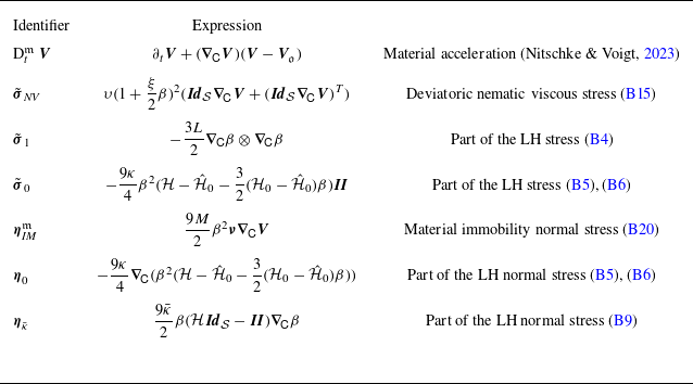


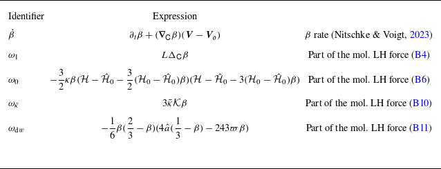


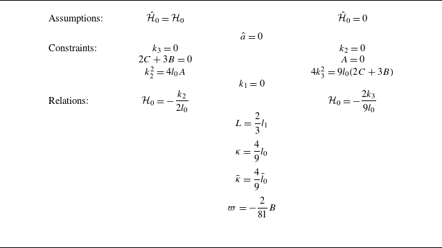


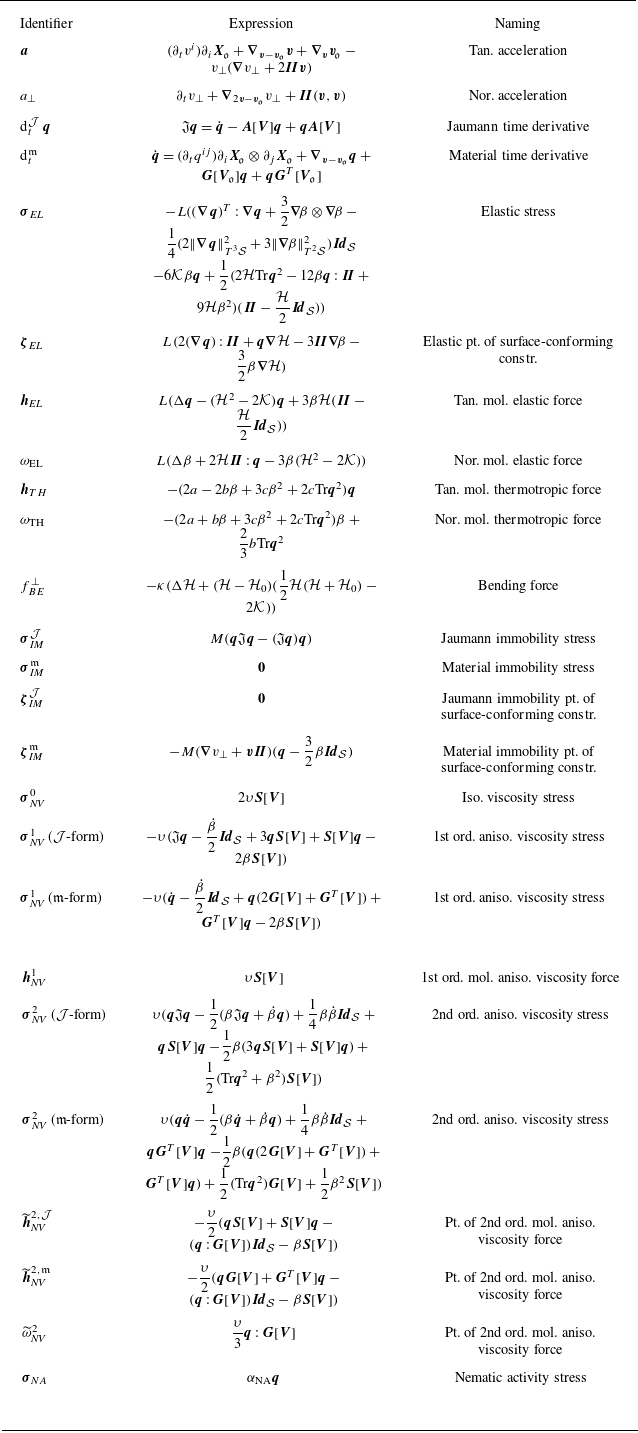


 Open access