


1. Introduction
It is easy to find equations and systems which lead to ill-posed problems (in the sense of Hadamard) when different models arisen in the applied mathematics are studied. Maybe the simplest way to find this problem is when we consider the backward in time heat equation, or the system of elasto-dynamics when the elasticity tensor is not positive definite. The spectra of these problems contain sequences whose elements have a real part which tends to infinity. Therefore, we cannot obtain the continuous dependence with respect to the initial data and, moreover, a certain norm of some solutions can blow up at finite time. So, it is important to know if, at least, we can ensure the uniqueness of solutions.
There are several techniques to study this kind of problems. We can cite the books of Ames and Straughan [Reference Ames and Straughan1] or Flavin and Rionero [Reference Flavin and Rionero5], where the authors recall different techniques to analyse them. They also study a series of problems arisen in applied mathematics. We can find in these books a huge quantity of references where qualitative properties of ill-posed problems are studied. One of the most used arguments in these works is the so-called logarithmic convexity.
We can also recall the works of Knops and Payne [Reference Knops and Payne7], where they obtained results of uniqueness and instability for elasto-dynamic problems (see also [Reference Galdi and Rionero6]), and which were extended by other authors to consider different thermoelastic theories [Reference Quintanilla and Straughan15, Reference Wilkes18]. In the book of Ames and Straughan [Reference Ames and Straughan1] we can find a full description of this method for the backward in time heat equation.
In the last years, a huge interest has been developed in the study of equations involving high order derivative in time. These appear in a natural way when we want to study different problems in the applied mathematics. Usually, parabolic and hyperbolic equations have been considered, leading to well-posed problems, and some results have been obtained [Reference Campo, Copetti, Fernández and Quintanilla2, Reference Magaña and Quintanilla11, Reference Quintanilla and Racke13]. However, few attention has been devoted to ill-posed problems associated to high order equations [Reference Dreher, Quintanilla and Racke4]. In this work, we aim to study one problem of this type. That is, we consider a kind of problem which is ill-posed and associated to high order equations. We think that this is the first contribution in this line.
Here, we consider an ill-posed problem (see equation (2.1) below) and we want to obtain a result concerning the uniqueness of solutions. Our argument is based on the method of logarithmic convexity. We have found two main difficulties to prove the main result. The first one is that it was not clear the function which we had to use. The second difficulty was that we had to bound different terms which must be controlled. In this work, we have overcome these difficulties with the help of a combination of integrals with respect to the time.
The plan for this paper is the following: in the next section we propose the problem to be studied and we state some few properties to be used later. In section three we prove the uniqueness result and, in section four, we recall three different situations where the above result can be applied. In the last section we propose further comments which allow to extend the results of the third section.
2. Preliminaries
Let us assume that $B$ represents a bounded domain in $\mathbb {R}^{d}$
 , for $d=1,\,2,\,3$
 .
.
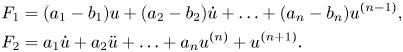
In this work, we are going to study uniqueness issues for the problem determined by the equation

where $a_i$ and $b_i$
 are real numbers, $n$
 is a natural number greater than zeroFootnote 1 and $k>0$
 , with the boundary condition
and the initial conditions, for a.e. $\boldsymbol {x}\in B$ ,
,

First, we must observe that this problem is not well posed in the sense of Hadamard. In particular, we will see that there exists a sequence of real numbers $\xi _n$ which tend to $+\infty$
 and belong to the point spectrum of this problem.
In fact, if we consider solutions of the form

where the function $\Phi _n(\boldsymbol {x})$ is the solution to the problem

then we find that the following relation

holds.
That is, $\omega$ satisfies the equation:

Our aim is to see that, when $\lambda _n$ tends to infinity, there exists a sequence of real numbers which are solutions to this equation $\xi _n$
 satisfying the condition $\lambda _n^{1/2}\leq \xi _n <\infty$
 such that $\xi _n\rightarrow \infty$
 when $\lambda _n\rightarrow \infty$
 .
.
First, we fix the value of $\lambda _n$ . Clearly, the function

tends to $+\infty$ when $x\rightarrow \infty$
 .
.
On the other hand, we can take the value of $P_k(x)$ for $x=\lambda _k^{1/2}$
 and so, we have

It is obvious that the term of highest order of the above polynomial is $-k\lambda _k^{\frac {n+2}{2}}.$
Therefore, if $\lambda _k$ is large enough, we find that $P_k(\lambda _k^{1/2})<0$
 and so, every $P_r(\lambda _r^{1/2})$
 , for $r\geq k$
 , are all negative. Now, applying mean value theorem we conclude that there exists $\xi _k$
 , $\lambda _k^{1/2}\leq \xi _k<\infty$
 , such that $P_k(\xi _k)=0$
 .
.
Clearly, for each large value of $\lambda _k$ we can choose $\xi _k$
 and, since $\lambda _k^{1/2}$
 tends to infinity, we may conclude that $\xi _k$
 also tends to infinity. Therefore, we have proved that problem (2.1)–(2.3) is ill-posed in the sense of Hadamard.
Remark 1 This analysis also applies if we consider the equation

in a Hilbert space $\mathcal {H}$ , where $A$
 is a symmetric and positive definite operator such that there exists an infinite sequence of eigenvalues $\lambda _n\rightarrow \infty$
 .
.
Now, since we have shown that the problem is not well-posed, we can ask ourselves about the uniqueness of solutions. Hence, it will be enough to prove that the unique solution when we consider the initial conditions

is the null solution.
Thus, our aim in the next section will be to prove that, under some assumptions, the unique solution to problems (2.1), (2.2) and (2.6) is the null solution. Therefore, it will be useful to recall some properties.
First, we recall the Poincaré-like inequality which states that the following estimate
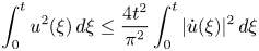
holds, whenever $u(0)=0$ .
.
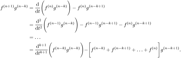
It will be also convenient to remark that
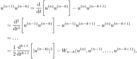
for $1\leq k < n$ , where $W_{n-k}$
 is a quadratic function in its arguments.
The relations (2.7) and (2.8) will be a key point in our study. From them, by using Hölder inequality we can conclude that
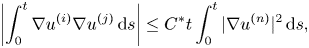
whenever $0\leq i,\,j\leq n$ , $i+j<2n$
 and (2.6) holds, where $C^{*}$
 is a computable constant.
From (2.7) and (2.9) we note that
where
$C_1$ is a positive calculable constant, and we have made a systematic use of the inequality (2.9), and for every constants $a_i$
 and $b_i$
 .
.
Finally, it is worth noting that if $u(0)=0$ then
then

In general, if we assume that conditions (2.6) are fulfilled, we can see that
for $2\leq j\leq n.$
3. Uniqueness of solutions
The objective of this section is to obtain an uniqueness result to problem (2.1)–(2.3).
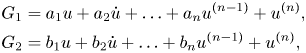
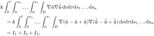
In order to simplify the notation, we can rewrite equation (2.1) in the form:

where $\tilde {u}=a_1u+a_2\dot {u}+\ldots +a_n u^{(n-1)}+u^{(n)}\ \hbox{and}\ \hat {u}=b_1u+b_2\dot {u}+\ldots +b_n u^{(n-1)}+u^{(n)}.$
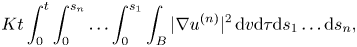
The main idea to prove the result will be to use the function
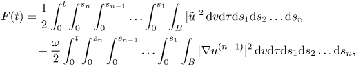
where $\omega$ is a positive constant which will be chosen later.
We have
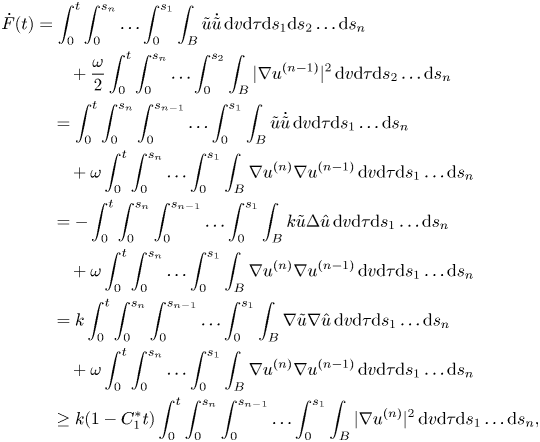
where we recall that $C_1^{*}$ is a positive calculable constant, and we have made a systematic use of the inequality (2.9).
We note that we can choose $T$ small enough to guarantee that
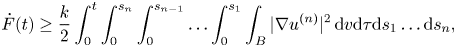
for every $t\leq T$ .
.
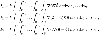
Now, we analyse the second derivative of the function $F$ . It follows thatFootnote 2
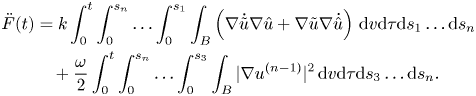
We can easily find that
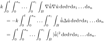
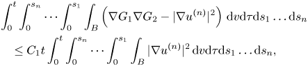
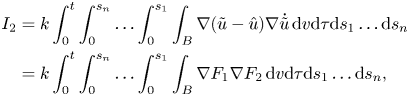
However, the second summand of the first integral in $\ddot {F}$ is more difficult to handle. We obtain that
where
We find that
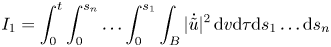
as we have seen previously.
On the other hand, we also have
where
We can bound the integrals of the form

by the integral
where $K$ is a computable constant, after a repetitive use of the inequality (2.9).
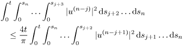
The terms more difficult to bound are those of the form

If we take into account that, for $j=1,\,\ldots,\,n-1,$

then we obtain
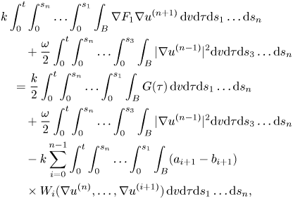
where
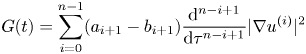
and $W_i$ is a quadratic expression of its arguments.
In view of the estimate (2.11) we see that the addition of the first and second terms on the right-hand side of (3.6) is positive whenever $t\leq T$ and $T$
 sufficiently small, and $\omega$
 large enough. Moreover, the third term on the right-hand side of (3.6) will be greater or equal to
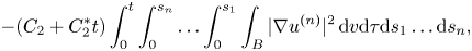
where constants $C_2$ and $C_2^{*}$
 can be easily calculated. Therefore, we find that
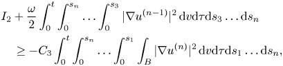
where $C_3$ is a computable constant for every $t\leq T$
 and $T$
 is small enough.
Thus, we have proved that

We bound now the integral $I_3$ . Proceeding in an analogous way, we also have

where $C_4$ is again a computable constant for every $t\leq T$
 , where $T$
 is sufficiently small.
Combining all these estimates, we conclude that, for every $t\leq T$ ,
,
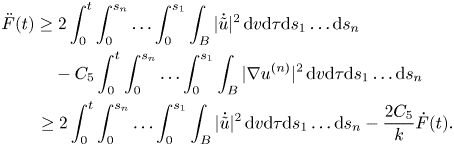
Therefore, if we assume that $t\leq T$ is small enough then we find that
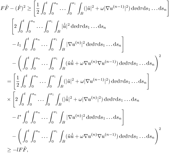
where $l_1$ , $l$
, $l$ and $l^{*}$
 are computable constants.
The inequality (3.8) is well-known in the study of the qualitative properties of the solutions to ill-posed problems. We find that (see [Reference Ames and Straughan1, Reference Flavin and Rionero5])

where $\sigma =e^{-lt}$ and $\sigma _2=e^{-lT}$
 . If we assume that the initial conditions are zero, then we obtain that $F(0)=0$
 and so, $F(t)=0$
 for a.e. $t\in [0,\,T]$
 . This implies that $u(t)=0$
 for a.e. $t\in [0,\,T].$
This process can be repeated successively in the interval $[T,\,2\,T]$ and so on. Therefore, we obtain that problem (2.1)–(2.3) has a unique solution.
Remark 2 Our analysis could be adapted to the problem proposed in remark 1. An elemental example could be

with the boundary conditions:

Another interesting example could be again the problem proposed in remark 1 when $Au=(b_{ij}(\boldsymbol {x}) u_{,i})_{,j}$ , where $b_{ij}(\boldsymbol {x})$
 is a symmetric positive definite tensor.
4. Applications to some special problems
In this section, we focus on the application of the result given in the previous section, related to the uniqueness of solution, to the generalized Burgers’ fluid, a couple of heat conduction problems and a viscoelastic problem. In particular, we aim to prove that, under certain conditions, it is not possible that the solutions to these three problems are localized in time. It means that, if the solution vanishes after a finite time $t_0\geq 0$ , then this solution is null. It is convenient to note that this property is equivalent to show that the backward in time problem has a unique solution.
4.1 Generalized Burgers’ fluid
In the paper [Reference Quintanilla and Rajagopal14] the authors proposed in a natural form the system which determines the evolution of the linearized form for the generalized Burgers’ fluid. We recall that it is written as follows,
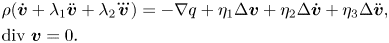
In the previous system, $\boldsymbol {v}$ is the velocity and $\lambda _1,\,\lambda _2,\, \eta _1,\, \eta _2,\, \eta _3$
 are positive constants. It is easy to rewrite this system as
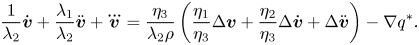
The backward in time problem is written in the following form:

Therefore, it leads to the following system:

This system is of the form:
where $k=\frac {\eta _3}{\lambda _2\rho }$ , $a_1=\lambda _2^{-1}$
 , $a_2=-\lambda _1\lambda _2^{-1}$
 , $b_1=\eta _1\eta _3^{-1}$
 and $b_2=-\eta _2\eta _3^{-1}$
 , and we adjoin null boundary conditions. Since we assume that $\rho$
 , $\lambda _2$
 and $\eta _3$
 are positive, then problem (4.1) is ill posed in the sense of Hadamard.
Thus, the arguments proposed previously can be adapted easily to this situation and we can conclude the uniqueness of solutions to the backward in time problem.
4.2 Dual-phase-lag and three-phase-lag heat conduction
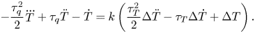
One of the theories proposed by Tzou [Reference Tzou17] considers the heat conduction equation:
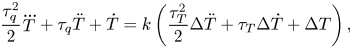
where $k>0$ and $\tau _q,\, \tau _T$
 are two positive relaxation parameters. The backward in time version of this equation is
We can write
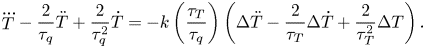
In view of the arguments of the previous section we can guarantee the uniqueness of solutions to this last equation with homogeneous Dirichlet boundary conditions.
In 2007, Roy Chouduri [Reference Choudhuri3] proposed the heat equation:

where $k$ and $k^{*}$
 are two positive parameters, $\tau _\nu ^{*}=k^{*}\tau _\nu +k$
 and $\tau _q,\, \tau _\nu$
 and $\tau _T$
 are three relaxation parameters. The backward in time version of this equation becomes
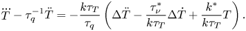
Therefore, we can guarantee the uniqueness of solutions to the problem determined by this equation with homogeneous Dirichlet boundary conditions.
4.3 Viscoelasticity
Lebedev and Gladwell [Reference Lebedev and Gladwell10] proposed a constitutive equation of the form:

where $A$ , $B$
, $B$ and $C$
 are polynomials, $\sigma _{ij}$
 is the stress tensor, $\varepsilon _{ij}$
 is the strain tensor and $\delta _{ij}$
 is the Kronecker symbol.
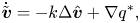
In the case that we consider anti-plane shear deformations and we assume that $degree(C)=degree(B)-1$ , we can obtain an equation of the form:

where $\mu >0$ . We can apply the results of the previous section to the backward in time version of this equation to conclude the impossibility of localization for the solutions to the equation (4.2). In fact, we could use the results for a more general version of viscoelasticity.
Viscoelastic fluids have deserved much attention in the last years. An interesting class of them can be found in [Reference Oskholkov and Shadiev12]. Linear and nonlinear versions have been studied [Reference Kalantarov and Titi8, Reference Kalantarov, Levant and Titi9, Reference Straughan16]. For some of them, the study we have developed can be used. For instance, the ones called of Oldroyd can be written as

where the parameters $\mu$ , $\gamma$
 and $\beta$
 are positive. The backward in time version of this equation can be written as
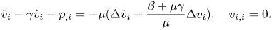
Therefore, our results apply to this case. However, it is suitable to recognize that our arguments cannot be used to study others viscoelastic fluids as the ones known as Kelvin–Voigt type.
5. Further comments
In the previous sections, we have assumed that $a_i$ and $b_j$
 are constants. The reason was that we needed it to prove that problem (2.1)–(2.3) is ill posed in the sense of Hadamard. However, in order to prove the uniqueness of solutions this assumption is not required as we will see below.
In what follows, we point out the changes in the proof that we need in the case that $a_i$ and $b_j$
 can depend on the point; however, we still assume that $k$
 is a constant. Anyway, we impose that $a_i$
 and $b_j$
 are $C^{1}$
 functions with respect to variable x.
It will be relevant to take into account an easy extension of the equality (2.8). We also have
Now, we develop the analysis. First, we note that the inequality (2.10) also holds in our case. We can define the function $F(t)$ as we have done in (3.1). Therefore, estimate (3.2) also holds. The unique difference is that we need to apply the Poincaré inequality at several points. We also have equality (3.3) where $I_i$
 are given in (3.4). Moreover, the equality (3.5) is satisfied but, again, the most difficult point is to estimate $I_2$
 . We have:
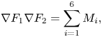
where
Again, integrals $M_i$ , $i=1,\,\ldots,\, 4$
 , can be controlled by expressions of the form:

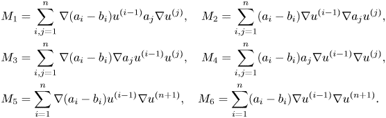
To estimate integral $M_6$ we can follow the same argument that in estimate (3.6) to obtain
where $\omega _1$ is large enough and $K_1$
 and $K_1^{*}$
 are constants whenever $t\leq T$
 and $T$
 is sufficiently small.
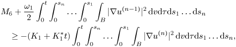
Using the equality (5.1) and the Poincaré inequality we can find that
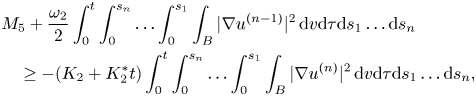
where, again, $\omega _2$ is large enough and $K_2$
 and $K_2^{*}$
 are constants when $t\leq T$
 for $T$
 sufficiently small.
Moreover, we can estimate $I_3$ as in (3.7) after the use of the Poincaré inequality.
Therefore, we can obtain once again an inequality of the type of (3.8) and so, we can conclude the uniqueness result proceeding as in § 3.
Acknowledgments
The authors thank Prof. Straughan for his valuable comments regarding the consequences of inequality (3.8). The authors also thank the anonymous reviewer whose comments have improved the final quality of the article. This paper is part of the projects PGC2018-096696-B-I00 and PID2019-105118GB-I00, funded by the Spanish Ministry of Science, Innovation and Universities and FEDER ‘A way to make Europe’.


 Open access