





1. Introduction
Gravity currents are generated by density differences and appear when a fluid of density $\rho$
advances into an ambient fluid of different density
$\rho$
advances into an ambient fluid of different density $\rho \pm \Delta \rho$
and the flow is primarily horizontal (Simpson Reference Simpson1997). Ungarish (Reference Ungarish2020) proposed a multifactor classification which makes it clear that several aspects of gravity-current dynamics remain insufficiently explored and warrant further investigation.
$\rho \pm \Delta \rho$
and the flow is primarily horizontal (Simpson Reference Simpson1997). Ungarish (Reference Ungarish2020) proposed a multifactor classification which makes it clear that several aspects of gravity-current dynamics remain insufficiently explored and warrant further investigation.
Among the outstanding issues, two are particularly relevant owing to their importance in industrial and environmental fluid mechanics: the influence of confinement and the role of surface tension effects. A central challenge lies in understanding how these two mechanisms interact, particularly in viscous gravity currents advancing under vertical confinement.
The significance of confinement was first established in the pioneering work of Nordbotten & Celia (Reference Nordbotten and Celia2006) on $\text{CO}_2$
injection into porous formations, after which successive studies refined this framework or introduced alternative conceptual models for natural porous-media applications (Gunn & Woods Reference Gunn and Woods2011; Dudfield & Woods Reference Dudfield and Woods2014; Farcas & Woods Reference Farcas and Woods2015; Guo et al. Reference Guo, Zheng, Celia and Stone2016; Pegler et al. Reference Pegler, Maskell, Daniels and Bickle2017). Vertical confinement is also crucial for free-fluid viscous gravity currents in industrial settings, such as injection moulding (Hoffman Reference Hoffman2014), thin-film coating and nasal drug delivery (Yang & Kowal Reference Yang and Kowal2025), as well as in environmental contexts (Taghavi et al. Reference Taghavi, Seon, Martinez and Frigaard2009; Zheng, Rongy & Stone Reference Zheng, Rongy and Stone2015). A comprehensive synthesis of confinement effects is provided in the review by Zheng & Stone (Reference Zheng and Stone2022).
$\text{CO}_2$
injection into porous formations, after which successive studies refined this framework or introduced alternative conceptual models for natural porous-media applications (Gunn & Woods Reference Gunn and Woods2011; Dudfield & Woods Reference Dudfield and Woods2014; Farcas & Woods Reference Farcas and Woods2015; Guo et al. Reference Guo, Zheng, Celia and Stone2016; Pegler et al. Reference Pegler, Maskell, Daniels and Bickle2017). Vertical confinement is also crucial for free-fluid viscous gravity currents in industrial settings, such as injection moulding (Hoffman Reference Hoffman2014), thin-film coating and nasal drug delivery (Yang & Kowal Reference Yang and Kowal2025), as well as in environmental contexts (Taghavi et al. Reference Taghavi, Seon, Martinez and Frigaard2009; Zheng, Rongy & Stone Reference Zheng, Rongy and Stone2015). A comprehensive synthesis of confinement effects is provided in the review by Zheng & Stone (Reference Zheng and Stone2022).
Among the industrial configurations where confinement and capillarity potentially interact, the study of Hoffman (Reference Hoffman2014) is particularly instructive. By numerically simulating mould-filling in thin geometries, the author showed that gravity can noticeably modify the advance of viscous fluids in narrow gaps, influencing how reliably the cavity is filled. This motivates considering simplified idealised settings in which a viscous fluid is injected into a thin horizontal gap of height $H$
representative of a long, shallow channel or a radially spreading layer. In such flows, the injected fluid may occupy the full gap over part of its extent while also forming a gravity-driven layer that spreads along the lower boundary, producing a coupled ‘slug–gravity-current’ structure. The relative development of these regions depends on the injection conditions, the gap height and the interplay between different forces.
$H$
representative of a long, shallow channel or a radially spreading layer. In such flows, the injected fluid may occupy the full gap over part of its extent while also forming a gravity-driven layer that spreads along the lower boundary, producing a coupled ‘slug–gravity-current’ structure. The relative development of these regions depends on the injection conditions, the gap height and the interplay between different forces.
Hutchinson, Gusinow & Worster (Reference Hutchinson, Gusinow and Worster2023) extended these ideas by examining the confined axisymmetric propagation of a Newtonian fluid through a combined theoretical and experimental study. Using lubrication theory, they showed that a constant injection rate leads to a self-similar spreading behaviour in which the dynamics depends on a single dimensionless parameter characterising the ratio between the gap height and the characteristic height of the corresponding unconfined gravity current. Experiments using golden syrup injected into an air-filled gap of roughly one centimetre confirmed the theoretical predictions, with some deviations.
Building on this work, Hutchinson (Reference Hutchinson2024) revisited the same axisymmetric configuration and showed that the observed discrepancies between theory and experiment can largely be attributed to the surface-tension effects at the grounding line. Although a complete Young–Laplace description predicts the formation of a meniscus whose height scales with the capillary length, the detailed shape and boundary conditions are sufficiently complex that a practical, fully resolved solution is not achievable. Instead, Hutchinson (Reference Hutchinson2024) introduced a simplified representation in which the meniscus is modelled as an effective vertical jump of the order of a fraction of the height of the gap. This modification allows surface tension to be incorporated straightforwardly into the lubrication framework. A key outcome is that the underlying similarity structure of the surface-tension-free model is preserved, while the quantitative relationships between the governing dimensionless groups are shifted in a manner consistent with experiments. Although the effective height of the meniscus cannot be precisely prescribed, the study showed that estimates based on the ratio between the capillary length and the height of the gap offer a reasonable approximation. This extended model was developed and validated for Newtonian fluids in axisymmetric geometry.
Additional insight into the influence of surface tension comes from Zheng, Christov & Stone (Reference Zheng, Christov and Stone2014), who reported that capillary forces may alter the far-field behaviour of convergent gravity currents to the extent that classical self-similar solutions no longer apply beyond a certain distance from the corner.
A further development is the extension to non-Newtonian rheology and multiple geometries. Ungarish (Reference Ungarish2025b
) generalised the confined-flow theory to both two-dimensional and axisymmetric configurations, and to power-law fluids with rheological index $n$
, recovering the Newtonian limit when
$n$
, recovering the Newtonian limit when $n=1$
. Within the lubrication framework, the author showed that self-similar spreading persists for specific injection laws determined by
$n=1$
. Within the lubrication framework, the author showed that self-similar spreading persists for specific injection laws determined by $n$
, with distinct spreading exponents in the two geometries. As in the Newtonian case, the detached portion of the current develops a sloping interface whose shape must be obtained from an ordinary differential equation with conditions at the nose and grounding line. When surface tension is neglected, the scaled solution depends on a single confinement parameter and the theory provides a clear prediction of the threshold below which the current behaves as effectively unconfined, advancing along the lower boundary without contacting the upper one.
$n$
, with distinct spreading exponents in the two geometries. As in the Newtonian case, the detached portion of the current develops a sloping interface whose shape must be obtained from an ordinary differential equation with conditions at the nose and grounding line. When surface tension is neglected, the scaled solution depends on a single confinement parameter and the theory provides a clear prediction of the threshold below which the current behaves as effectively unconfined, advancing along the lower boundary without contacting the upper one.
The present study builds on previous research in two complementary directions. First, it develops analytical solutions for vertically confined gravity currents of power-law fluids between parallel plates and with time-dependent injected volume, incorporating surface-tension effects at the grounding line, modelled as a vertical discontinuity of size $\sigma H$
following the approach of Hutchinson (Reference Hutchinson2024), where
$\sigma H$
following the approach of Hutchinson (Reference Hutchinson2024), where $\sigma =\mathcal{O}(S)$
and
$\sigma =\mathcal{O}(S)$
and $S =l/H\equiv (\varGamma /\rho g\prime)^{1/2}/H$
, with
$S =l/H\equiv (\varGamma /\rho g\prime)^{1/2}/H$
, with $\varGamma$
the surface tension,
$\varGamma$
the surface tension, $l$
the capillary length,
$l$
the capillary length, $g\prime=(\Delta \rho /\rho ) g$
the reduced gravity and
$g\prime=(\Delta \rho /\rho ) g$
the reduced gravity and $H$
the distance between the parallel plates. In doing so, it refines the framework of Ungarish (Reference Ungarish2025b
) by explicitly accounting for surface tension and extends the methodology of Hutchinson (Reference Hutchinson2024) to non-Newtonian fluids. Second, and constituting the main contribution, it provides experimental insight into the flow and assesses the accuracy of the theoretical predictions through a series of controlled tests with non-Newtonian fluids, including comprehensive rheological characterisation, thereby generalising the experimental methodology of Hutchinson et al. (Reference Hutchinson, Gusinow and Worster2023) to non-Newtonian fluids.
$H$
the distance between the parallel plates. In doing so, it refines the framework of Ungarish (Reference Ungarish2025b
) by explicitly accounting for surface tension and extends the methodology of Hutchinson (Reference Hutchinson2024) to non-Newtonian fluids. Second, and constituting the main contribution, it provides experimental insight into the flow and assesses the accuracy of the theoretical predictions through a series of controlled tests with non-Newtonian fluids, including comprehensive rheological characterisation, thereby generalising the experimental methodology of Hutchinson et al. (Reference Hutchinson, Gusinow and Worster2023) to non-Newtonian fluids.
An additional experimentally driven objective concerns the early-time behaviour of the gravity current, during which the similarity solution is expected to be inapplicable (Barenblatt Reference Barenblatt1996). Our results indicate that surface tension plays a key role in the hysteresis observed during these initial stages, controlling the transition between confined and unconfined flow regimes. The experiments were particularly challenging, requiring the simultaneous determination of the positions of the two fronts as well as precise measurements of the rheometric parameters and surface tension.
It should be noted that surface tension is also expected to generate a meniscus at the nose of the current, corresponding to a modification of the tip of the gravity current at the lower boundary, $r_N(t)$
in figure 1. This effect could, in principle, be incorporated into the similarity solution through an additional small parameter,
$r_N(t)$
in figure 1. This effect could, in principle, be incorporated into the similarity solution through an additional small parameter, $\sigma _N$
. However, there is theoretical evidence (as specified later) that the influence of the nose meniscus is generally much smaller than that of the grounding-line meniscus; accordingly, in this study, we deliberately neglect its presence in the main analysis and discussion.
$\sigma _N$
. However, there is theoretical evidence (as specified later) that the influence of the nose meniscus is generally much smaller than that of the grounding-line meniscus; accordingly, in this study, we deliberately neglect its presence in the main analysis and discussion.
The manuscript is organised as follows. Section 2 presents the mathematical model and discusses the influence of surface tension in both two-dimensional and axisymmetric configurations. Section 3 describes the experimental set-up and analyses the corresponding results. Section 4 focuses on surface-tension-induced hysteresis phenomena, highlighting their dependence on the geometry of the experimental apparatus and on the test protocol. Section 5 provides a summary of the main findings and concluding remarks. Finally, the Appendix presents the assessment of the relevant shear-rate interval, carried out separately for the free-surface and confined regions of the gravity current (GC).
2. Theory
2.1. Mathematical model
The system of the gravity current (GC) is as sketched in figure 1. A three-dimensional (3-D) axisymmetric viscous GC of density $\rho$
propagates within the confined gap between two horizontal parallel plates separated by distance
$\rho$
propagates within the confined gap between two horizontal parallel plates separated by distance $H$
, displacing an ambient fluid with density
$H$
, displacing an ambient fluid with density $\rho -\Delta \rho$
. The radii of the grounding line and the nose are
$\rho -\Delta \rho$
. The radii of the grounding line and the nose are $r_G(t)$
and
$r_G(t)$
and $r_N(t)$
, respectively. The formulation for viscous power law GCs without surface tension (
$r_N(t)$
, respectively. The formulation for viscous power law GCs without surface tension ( $\varGamma =0\to \sigma = 0$
) is presented by Ungarish (Reference Ungarish2025b
). Here, we briefly summarise the extension for the system affected by the surface tension.
$\varGamma =0\to \sigma = 0$
) is presented by Ungarish (Reference Ungarish2025b
). Here, we briefly summarise the extension for the system affected by the surface tension.
Sketch of the confined system: lubrication model for the GC with inclined interface. The height of the meniscus at the grounding line is $\sigma H$
. The volume (per radian) is
$\sigma H$
. The volume (per radian) is $\mathcal{V} = q t^\alpha$
. In the self-similar flow,
$\mathcal{V} = q t^\alpha$
. In the self-similar flow, $r_G = y_G K t^\beta$
,
$r_G = y_G K t^\beta$
, $r_N= K t^\beta$
and
$r_N= K t^\beta$
and $r_G$
depends on the parameters
$r_G$
depends on the parameters $J$
and
$J$
and $\sigma$
.
$\sigma$
. $\alpha , \beta , K, y_G$
are positive constants.
$\alpha , \beta , K, y_G$
are positive constants.

Figure 1. Long description
A sketch of a confined system showing a lubrication model for a gravity current with an inclined interface. The diagram includes a meniscus at the grounding line with a height denoted by sigma H. The volume per radian is represented by the integral of h(r, t) times r dr from r_G(t) to r_N(t). In the self-similar flow, r_G(t) is proportional to t to the power of alpha, and r_N(t) is proportional to t to the power of beta. The parameters alpha and beta depend on the given parameters, and k1 and k2 are positive constants. The influx is shown entering the system from the left side, and the height of the system is denoted by H. The density of the fluid is represented by rho, and the reduced density is represented by rho - delta rho. The gravitational force is indicated by g pointing downward.
The mathematical model is based on several key simplifying assumptions: (i) the flow is axisymmetric-divergent from the origin in the cylindrical system, i.e. depending on the $r,z$
coordinates (with no lateral velocity component); (ii) the flow of the ambient fluid is neglected, which is justified when the density and viscosity of the displaced fluid are significantly smaller than those of the GC. The interface between the fluids is expected to be stable with respect to the Taylor– Saffman effect and the reduced pressure,
$r,z$
coordinates (with no lateral velocity component); (ii) the flow of the ambient fluid is neglected, which is justified when the density and viscosity of the displaced fluid are significantly smaller than those of the GC. The interface between the fluids is expected to be stable with respect to the Taylor– Saffman effect and the reduced pressure, $p$
, in the ambient fluid is constant (for definiteness, set to 0); (iii) the GC in the domain
$p$
, in the ambient fluid is constant (for definiteness, set to 0); (iii) the GC in the domain $r_G(t) \lt r \le r_N(t)$
is a thin viscous layer of height
$r_G(t) \lt r \le r_N(t)$
is a thin viscous layer of height $h(r,t) \lt H$
, which admits the approximation of the lubrication theory (see, e.g. Ungarish Reference Ungarish2020); (iv) at the grounding line
$h(r,t) \lt H$
, which admits the approximation of the lubrication theory (see, e.g. Ungarish Reference Ungarish2020); (iv) at the grounding line $r=r_G(t)$
, the interface of the GC is attached to the top by a vertical jump of height
$r=r_G(t)$
, the interface of the GC is attached to the top by a vertical jump of height $\sigma H$
, which represents a surface tension meniscus. The real shape of the meniscus is readily identified in some snapshots of the experiments presented later.
$\sigma H$
, which represents a surface tension meniscus. The real shape of the meniscus is readily identified in some snapshots of the experiments presented later.
We assume that $\sigma \leqslant 0.5$
(roughly, the capillary length is smaller than
$\sigma \leqslant 0.5$
(roughly, the capillary length is smaller than $0.5H$
), in which case, the surface tension may be significant, but is not the dominant effect (as shown later). When surface tension is negligible,
$0.5H$
), in which case, the surface tension may be significant, but is not the dominant effect (as shown later). When surface tension is negligible, $\sigma =0$
. The real meniscus has a curved interface (determined by the solution of the Young–Laplace equation as mentioned previously, and as experimentally observed in some snapshots presented in the following). The typical radial extent of the meniscus is of the order of
$\sigma =0$
. The real meniscus has a curved interface (determined by the solution of the Young–Laplace equation as mentioned previously, and as experimentally observed in some snapshots presented in the following). The typical radial extent of the meniscus is of the order of $H \ll r_N$
and, hence, the representation of the meniscus by a vertical jump is a consistent thin-layer approximation (we recall that the possible meniscus at the nose is presently ignored; this effect will be considered later in § 2.3).
$H \ll r_N$
and, hence, the representation of the meniscus by a vertical jump is a consistent thin-layer approximation (we recall that the possible meniscus at the nose is presently ignored; this effect will be considered later in § 2.3).
In summary, a more detailed treatment of the moving contact-line dynamics at $r_G$
and
$r_G$
and $r_N$
is omitted, an assumption that is appropriate for the viscous–gravity-dominated regime characteristic of the present configuration.
$r_N$
is omitted, an assumption that is appropriate for the viscous–gravity-dominated regime characteristic of the present configuration.
The analysis can be performed in a convenient compact form for both Newtonian and non-Newtonian (power-law) fluids. We use dimensional variables unless stated otherwise.
The dynamic viscosity of the current is given by
 \begin{equation} \mu = m \left | \frac {\partial u}{\partial z} \right | ^{n -1}, \end{equation}
where $m$
is the consistency index and
$m$
is the consistency index and $n$
is the fluid behaviour index (or exponent). We can also define
$n$
is the fluid behaviour index (or exponent). We can also define $\nu = m/\rho$
of dimensions [
$\nu = m/\rho$
of dimensions [ $\text{L}^2 \text{T} ^{n-2}$
]. A fluid is shear-thinning (pseudoplastic) if
$\text{L}^2 \text{T} ^{n-2}$
]. A fluid is shear-thinning (pseudoplastic) if $n \lt 1$
, shear-thickening (dilatant) if
$n \lt 1$
, shear-thickening (dilatant) if $n \gt 1$
and Newtonian if
$n \gt 1$
and Newtonian if $n=1$
(in this case,
$n=1$
(in this case, $m = \mu$
, the standard dynamic viscosity of the fluid and
$m = \mu$
, the standard dynamic viscosity of the fluid and $\nu$
is the standard kinematic viscosity coefficient). In the one-dimensional approximation adopted, the shear stress is given by
$\nu$
is the standard kinematic viscosity coefficient). In the one-dimensional approximation adopted, the shear stress is given by $\tau _{zr}\equiv \tau =\mu (\dot {\gamma } ) \dot {\gamma }=m| \partial u/\partial z|^{n -1} \partial u/\partial z$
, where
$\tau _{zr}\equiv \tau =\mu (\dot {\gamma } ) \dot {\gamma }=m| \partial u/\partial z|^{n -1} \partial u/\partial z$
, where $\dot {\gamma }$
is the shear rate. The power-law model was chosen over more sophisticated rheological models, such as the Ellis and Carreau–Yasuda models, for pragmatic reasons. The aim was to limit the number of rheological parameters and the overall complexity of the analysis while still capturing the essential non-Newtonian behaviour of the fluids. It is important to note that the power-law model, particularly for shear-thinning fluids, can perform poorly at low shear-rates, where it predicts an apparent viscosity that diverges; see, e.g. Longo et al. (Reference Longo, Di Federico, Archetti, Chiapponi, Ciriello and Ungarish2013a
), Picchi et al. (Reference Picchi, Ullmann, Brauner and Poesio2021), Boyko & Stone (Reference Boyko and Stone2021). In the present framework, the power-law approximation is appropriate when the combination of propagation distance, inflow rate–time exponent and gap height ensures that the shear rates remain within the range over which the rheological behaviour is well described by a power-law based on rheometric measurements. The lowest shear-rate values are expected near the nose; the slower the nose during injection, the lower the shear rates and the greater the potential for reduced accuracy. Details on the assessment of the relevant shear-rate interval, distinguishing between the free-surface and confined regions of the gravity current, are provided in the Appendix.
$\dot {\gamma }$
is the shear rate. The power-law model was chosen over more sophisticated rheological models, such as the Ellis and Carreau–Yasuda models, for pragmatic reasons. The aim was to limit the number of rheological parameters and the overall complexity of the analysis while still capturing the essential non-Newtonian behaviour of the fluids. It is important to note that the power-law model, particularly for shear-thinning fluids, can perform poorly at low shear-rates, where it predicts an apparent viscosity that diverges; see, e.g. Longo et al. (Reference Longo, Di Federico, Archetti, Chiapponi, Ciriello and Ungarish2013a
), Picchi et al. (Reference Picchi, Ullmann, Brauner and Poesio2021), Boyko & Stone (Reference Boyko and Stone2021). In the present framework, the power-law approximation is appropriate when the combination of propagation distance, inflow rate–time exponent and gap height ensures that the shear rates remain within the range over which the rheological behaviour is well described by a power-law based on rheometric measurements. The lowest shear-rate values are expected near the nose; the slower the nose during injection, the lower the shear rates and the greater the potential for reduced accuracy. Details on the assessment of the relevant shear-rate interval, distinguishing between the free-surface and confined regions of the gravity current, are provided in the Appendix.
The GC propagates in the $r$
direction with velocity
$r$
direction with velocity $u(r,z,t)$
and let
$u(r,z,t)$
and let $z=h(r,t)$
be the height of the interface above the bottom. The pressure in the thin-layer GC is hydrostatic,
$z=h(r,t)$
be the height of the interface above the bottom. The pressure in the thin-layer GC is hydrostatic, $p = g \Delta \rho (h-z)$
, where
$p = g \Delta \rho (h-z)$
, where $g$
is the gravity acceleration. Therefore, the intrinsic driving force is given by
$g$
is the gravity acceleration. Therefore, the intrinsic driving force is given by $-g\prime (\partial h /\partial r)$
, called the buoyancy. The effects of surface tension on the driving force are negligible because the interface is much larger than the
$-g\prime (\partial h /\partial r)$
, called the buoyancy. The effects of surface tension on the driving force are negligible because the interface is much larger than the $\sigma H$
meniscus. The buoyancy driving force is balanced by the shear, as expressed by the following lubrication-simplification momentum equation:
$\sigma H$
meniscus. The buoyancy driving force is balanced by the shear, as expressed by the following lubrication-simplification momentum equation:
 \begin{equation} g\prime \frac {\partial h}{\partial r} - \nu \frac {\partial }{\partial z} \left [ \left | \frac {\partial u}{\partial z} \right | ^{n -1} \frac {\partial u}{\partial z } \right ]=0. \end{equation}
This equation is integrated twice with respect to $z$
to obtain
$z$
to obtain $u(r,z,t)$
. The integration constants are determined by the boundary condition: (i) no slip
$u(r,z,t)$
. The integration constants are determined by the boundary condition: (i) no slip $u=0$
at the bottom
$u=0$
at the bottom $z=0$
and (ii) no shear,
$z=0$
and (ii) no shear, $(\partial u /\partial z) = 0$
, at the free interface
$(\partial u /\partial z) = 0$
, at the free interface $z = h,\quad r_G\lt r\lt r_N$
. We obtain
$z = h,\quad r_G\lt r\lt r_N$
. We obtain
 \begin{equation} u(r,z,t) = \frac {n}{n+1}\mathcal{G}^{1/n} \left (- \frac {\partial h}{\partial r} \right )^{1/n} h^{(n+1)/n} \left [ 1 - \left (1 - \frac {z}{h} \right ) ^{(n+1)/n} \right ], \end{equation}
where
 \begin{equation} \mathcal{G} = g\prime/\nu . \end{equation}
The depth-averaged velocity is
 \begin{equation} \bar {u}(r,t) = \frac {1}{h} \int _0^h u(r,z,t) \,\text{d}z = \frac {n}{2n+1} \mathcal{G}^{1/n} \left (- \frac {\partial h}{\partial r} \right )^{1/n} h^{(n+1)/n} . \end{equation}
The continuity equation is
 \begin{equation} \frac {\partial h}{\partial t}+ \frac {1}{r} \frac {\partial }{\partial r} ( {h} r \bar {u}) = 0. \end{equation}
In the following, we drop the upper bar in $\bar {u}$
and, unless stated otherwise, we refer to
$\bar {u}$
and, unless stated otherwise, we refer to $u$
as the depth-averaged velocity. The continuity equation and (2.5) form a set of equations for
$u$
as the depth-averaged velocity. The continuity equation and (2.5) form a set of equations for $u(r,t)$
and
$u(r,t)$
and $h(r,t)$
. The boundary conditions at the nose
$h(r,t)$
. The boundary conditions at the nose $r_N$
are
$r_N$
are $h_N =0$
while
$h_N =0$
while ${u}_N = {\rm d} r_N /\text{d}t$
. These conditions are not affected by the meniscus at the grounding line.
${u}_N = {\rm d} r_N /\text{d}t$
. These conditions are not affected by the meniscus at the grounding line.
As noted by Hutchinson et al. (Reference Hutchinson, Gusinow and Worster2023), Hutchinson (Reference Hutchinson2024) and Ungarish (Reference Ungarish2025b
), the effect of the confining boundary enters the mathematical model of the GC as a flux condition, $r h u$
, at the moving grounding line. The presence of the meniscus affects this condition because
$r h u$
, at the moving grounding line. The presence of the meniscus affects this condition because $h = (1-\sigma )H$
at
$h = (1-\sigma )H$
at $r_G^+(t)$
. The necessary flux condition is derived as follows.
$r_G^+(t)$
. The necessary flux condition is derived as follows.
Conservation of the total volume (per radian) is
 \begin{equation} \mathcal{V} = \frac {1}{2} r_G^2 H + \int _{r_G^+(t)}^{r_N(t)} h(r,t) r\, \text{d}r = q t^ \alpha , \end{equation}
where $q$
is a positive coefficient, which describes the inflow rate (per radian) through the relation
$q$
is a positive coefficient, which describes the inflow rate (per radian) through the relation $\dot {V}=\alpha q t^{\alpha -1}.$
We apply
$\dot {V}=\alpha q t^{\alpha -1}.$
We apply $t$
derivative to (2.7) and use (2.6) to eliminate
$t$
derivative to (2.7) and use (2.6) to eliminate $\partial h/\partial t$
. Recalling
$\partial h/\partial t$
. Recalling $h_N =0$
and
$h_N =0$
and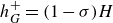 $h_G^+ = (1-\sigma )H$
, we obtain the flux condition at
$h_G^+ = (1-\sigma )H$
, we obtain the flux condition at $r_G^+$
,
$r_G^+$
,
 \begin{equation} \sigma r_G \frac {\text{d}r_G}{\text{d}t}H + (r h u)_G = \alpha q t^{\alpha - 1}. \end{equation}
2.1.1. Dimensionless formulation
We switch to dimensionless variables. The lengths are scaled with $H$
and the volume (per radian) with
$H$
and the volume (per radian) with $H^3$
. The scales for velocity, time and flux coefficient are as follows:
$H^3$
. The scales for velocity, time and flux coefficient are as follows:
 \begin{equation} U = \frac {n}{2n +1} \mathcal{G}^{1/n} H ^{(n+1)/n}, \quad T = \frac {H}{U}, \quad Q_{\textit{scale}} = \frac {H^3}{T^\alpha } \equiv H^{(3n + \alpha )/n} \left ( \frac {n}{2n +1} \right )^\alpha \mathcal{G}^{\alpha /n}. \end{equation}
Subsequently, in this section, unless otherwise stated, the variables $r, t, h, u, \mathcal{V}$
and
$r, t, h, u, \mathcal{V}$
and $q$
are dimensionless, scaled as defined previously. The dimensional counterpart, when needed, will be denoted by an asterisk; in particular, we note that the dimensional flux coefficient, which will appear in the definition of
$q$
are dimensionless, scaled as defined previously. The dimensional counterpart, when needed, will be denoted by an asterisk; in particular, we note that the dimensional flux coefficient, which will appear in the definition of $J$
, is denoted
$J$
, is denoted $q^\ast$
. The insight from the previous solution with no surface tension (
$q^\ast$
. The insight from the previous solution with no surface tension ( $\sigma = 0$
) suggests that the convenient parameter for expressing the importance of flow confinement is the dimensionless flux coefficient
$\sigma = 0$
) suggests that the convenient parameter for expressing the importance of flow confinement is the dimensionless flux coefficient $q$
at some power. We note the scaling
$q$
at some power. We note the scaling $Q_{\textit{scale}} \propto H^{(3 n + \alpha )/n}$
and this suggests the use of the following parameter:
$Q_{\textit{scale}} \propto H^{(3 n + \alpha )/n}$
and this suggests the use of the following parameter:
 \begin{equation} J = q ^{n/( 3 n + \alpha )} \equiv \left [ \left ( \frac {2n +1}{n} \right )^\alpha q^\ast \mathcal{G}^{-\alpha /n} \right ]^{n/( 3 n + \alpha )} \frac {1}{H}=\frac {L}{H}. \end{equation}
The right-hand side of (2.10) is the ratio of a length, $L$
, to
$L$
, to $H$
. This expresses the ratio of the typical thickness of the unconfined GC to
$H$
. This expresses the ratio of the typical thickness of the unconfined GC to $H$
.
$H$
.
2.2. The similarity solution
The dimensionless depth-averaged velocity is
 \begin{equation} {u}(r,t) = \left (- \frac {\partial h}{\partial r} \right )^{1/n} h^{(n+1)/n} . \end{equation}
We substitute (2.11) into the continuity equation (2.6) and introduce the reduced horizontal coordinate of the GC,
 \begin{equation} y = r/r_N(t), \end{equation}
where $0\lt y\le 1$
. The governing equation of the GC, in terms of
$0\lt y\le 1$
. The governing equation of the GC, in terms of $y$
and
$y$
and $t$
, reads as follows:
$t$
, reads as follows:
 \begin{equation} \frac {\partial h}{\partial t} - y \frac {\dot {r}_N}{r_N}\frac {\partial h}{\partial y} + \frac {1}{r_N^{(n+1)/n}}\frac {1}{y}\frac {\partial }{\partial y}\left [ yh^{(2n+1)/n}\left (-\frac {\partial h}{\partial y}\right )^{1/n}\right ]=0, \end{equation}
where the upper dot denotes the time derivative. The nose of the GC is at $y=1$
, where the boundary condition is
$y=1$
, where the boundary condition is
 \begin{equation} h=0\quad \text{for}\quad y=1, \end{equation}
and the grounding line is at $y_G$
, where the following boundary condition holds:
$y_G$
, where the following boundary condition holds:
 \begin{equation} h=1-\sigma \quad \text{for}\quad y=y_G. \end{equation}
The solution of (2.13) is of interest in the domain $y_G \le y \le 1$
. We argue that the cases of interest must have a constant
$y_G \le y \le 1$
. We argue that the cases of interest must have a constant $y_G \in (0,1)$
; otherwise,
$y_G \in (0,1)$
; otherwise, $y_G$
will migrate to either
$y_G$
will migrate to either $0$
(unconfined GC) or
$0$
(unconfined GC) or $1$
(full slug). Such a non-trivial system appears when both
$1$
(full slug). Such a non-trivial system appears when both $r_G$
and
$r_G$
and $r_N$
propagate like
$r_N$
propagate like $t^\beta$
, where
$t^\beta$
, where $\beta$
is a constant.
$\beta$
is a constant.
We therefore attempt a similarity solution of the form
 \begin{align}&\qquad\qquad\qquad\qquad r_N(t) = K t^\beta , \quad r_G(t) = y_G K t^\beta , \end{align}
 \begin{align}& h(y,t) = h(y) = K^{(n+1)/(n+2)} \lambda (y), \quad u(y,t) = [ \lambda ^{n+1} (- \lambda^{\prime}) ]^{1/n}K t^{\beta -1}, \end{align}
where the prime denotes derivative with respect to $y$
. The choice
$y$
. The choice $h= h(y)$
means that the current elongates with time, but maintains the thickness at the points
$h= h(y)$
means that the current elongates with time, but maintains the thickness at the points $y = r/r_N$
. This special form of
$y = r/r_N$
. This special form of $h$
follows from the observation that
$h$
follows from the observation that $h$
must be constant,
$h$
must be constant, $1-\sigma$
, at the grounding-line position
$1-\sigma$
, at the grounding-line position $y=y_G$
. The variable
$y=y_G$
. The variable $\lambda (y)$
represents the thickness (height) of the GC. The scaling of this variable renders some benefits which will be seen later.
$\lambda (y)$
represents the thickness (height) of the GC. The scaling of this variable renders some benefits which will be seen later.
The existence of the similarity solution is not guaranteed a priori. We must demonstrate that the postulated flow satisfies the equations and boundary conditions with physical values of $\beta$
and
$\beta$
and $K$
.
$K$
.
For a given $n$
, the substitution of the similarity behaviour (2.16) into the continuity equation (2.13) imposes the condition
$n$
, the substitution of the similarity behaviour (2.16) into the continuity equation (2.13) imposes the condition
 \begin{equation} \alpha = \frac {2n}{n+1}, \quad \beta = \dfrac {\alpha }{2} \equiv \frac {n}{n+1}, \end{equation}
and yields the equation
 \begin{equation} \left [ y\lambda ^{(2n+1)/n} \left (- \lambda^{\prime} \right )^{1/n} \right ]^{\prime} - \beta y^2\lambda ^{\prime} = 0, \end{equation}
where the prime symbol indicates derivation. The nose condition $\lambda (1) = 0$
(i.e.
$\lambda (1) = 0$
(i.e. $h_N=0$
) justifies the Frobenius-series result
$h_N=0$
) justifies the Frobenius-series result
 \begin{equation} \lambda (y) = \left [ (n + 2) \beta ^n (1-y) \right ] ^{1/(n+2)} \equiv \left [ (n + 2) \left ( \frac {n }{n+1} \right ) ^n (1-y) \right ] ^{1/(n+2)} \, (y \to 1). \end{equation}
This provides values of $\lambda$
and
$\lambda$
and $\lambda^{\prime}$
at
$\lambda^{\prime}$
at $y =1 - \varDelta$
, for a small
$y =1 - \varDelta$
, for a small $\varDelta$
, which allow numerical integration of (2.18) to smaller
$\varDelta$
, which allow numerical integration of (2.18) to smaller $y$
. We conclude that the height profile
$y$
. We conclude that the height profile $\lambda (y)$
of the interface of the GC for
$\lambda (y)$
of the interface of the GC for $y \in (y_0,1)$
can be obtained by a standard numerical method (we used fourth-order Runge–Kutta;
$y \in (y_0,1)$
can be obtained by a standard numerical method (we used fourth-order Runge–Kutta; $y_0$
is a small number which mimics the finite radius of the source, we used 0.05). This
$y_0$
is a small number which mimics the finite radius of the source, we used 0.05). This $\lambda (y)$
we call ‘general (or universal) profile’ because it does not depend on
$\lambda (y)$
we call ‘general (or universal) profile’ because it does not depend on $J$
and
$J$
and $\sigma$
(only on
$\sigma$
(only on $n$
). Actually, this is the profile of an unconfined GC with influx power
$n$
). Actually, this is the profile of an unconfined GC with influx power $\alpha$
given by (2.17).
$\alpha$
given by (2.17).
Next, we consider the flux boundary condition (2.8). We find that this condition, applied at a fixed $y_G$
, is compatible with the similarity assumption (2.16) when
$y_G$
, is compatible with the similarity assumption (2.16) when $\beta = \alpha /2$
(independent of the value of
$\beta = \alpha /2$
(independent of the value of $\sigma$
).
$\sigma$
).
The calculation of $J$
and
$J$
and $K$
can now be performed for a given pair of
$K$
can now be performed for a given pair of $y_G$
and
$y_G$
and $\sigma$
. At position
$\sigma$
. At position $y=y_G$
, where
$y=y_G$
, where $\lambda _G$
and
$\lambda _G$
and $\lambda^{\prime}_G$
are known (from the general profile), we apply the grounding-line condition (2.15) and volume flux (2.8). After some algebra, this yields the following:
$\lambda^{\prime}_G$
are known (from the general profile), we apply the grounding-line condition (2.15) and volume flux (2.8). After some algebra, this yields the following:
 \begin{align}&\qquad\qquad\quad K = \left [ (1-\sigma )/ \lambda _G \right ] ^{(n+2)/(n+1)}, \end{align}
 \begin{align} q &= J ^{3 + \alpha /n} \equiv (K^2 y_G/\alpha ) \left [(1-\sigma ) (- \lambda^{\prime}_G \lambda _G^{n+1}) ^{1/n} + \beta \sigma y_G \right ]\!. \end{align}
For given $n$
,
$n$
, $\sigma$
and
$\sigma$
and $y_G$
, we obtain the values of
$y_G$
, we obtain the values of $J$
and
$J$
and $K$
of the confined GC. For
$K$
of the confined GC. For $\sigma = 0$
, we recover the results of Ungarish (Reference Ungarish2025b
). Physically acceptable results were obtained for all tests in the plausible parameter range of
$\sigma = 0$
, we recover the results of Ungarish (Reference Ungarish2025b
). Physically acceptable results were obtained for all tests in the plausible parameter range of $n, \sigma$
and
$n, \sigma$
and $y_G \in (0.05, 0.99)$
. This confirms the validity of the similarity solution. The point
$y_G \in (0.05, 0.99)$
. This confirms the validity of the similarity solution. The point $y_G = 0.05$
, where
$y_G = 0.05$
, where $J=J_0$
, is considered the onset of the confinement effect; GCs with
$J=J_0$
, is considered the onset of the confinement effect; GCs with $J\lt J_0$
are considered free (unconfined) and outside the scope of the present work. The results of Hutchinson et al. (Reference Hutchinson, Gusinow and Worster2023) and Hutchinson (Reference Hutchinson2024) are recovered for
$J\lt J_0$
are considered free (unconfined) and outside the scope of the present work. The results of Hutchinson et al. (Reference Hutchinson, Gusinow and Worster2023) and Hutchinson (Reference Hutchinson2024) are recovered for $n=1$
(but note that these papers use a different scaling of the variables).
$n=1$
(but note that these papers use a different scaling of the variables).
It is remarkable that the presence of the meniscus $\sigma \gt 0$
has little effect on the theoretical flow pattern. The similarity behaviour of the grounding line and nose position,
$\sigma \gt 0$
has little effect on the theoretical flow pattern. The similarity behaviour of the grounding line and nose position, $\sim t^\beta$
, for select values of
$\sim t^\beta$
, for select values of $\alpha$
, are the same as for
$\alpha$
, are the same as for $\sigma = 0$
. The variables
$\sigma = 0$
. The variables $K, J$
and
$K, J$
and $y_G$
depend on
$y_G$
depend on $\sigma$
. In the domain
$\sigma$
. In the domain $r_G(t) \lt r \le r_N(t)$
, the height profile
$r_G(t) \lt r \le r_N(t)$
, the height profile $\lambda (y)$
of the interface of the GC is also unaffected and actually the same as for an unconfined GC.
$\lambda (y)$
of the interface of the GC is also unaffected and actually the same as for an unconfined GC.
We emphasise that the similarity solution for the confined GC exists only for the select values of $\alpha$
given by (2.17). The corresponding influx is able to sustain the grounding line height
$\alpha$
given by (2.17). The corresponding influx is able to sustain the grounding line height $h = 1-\sigma$
at a fixed
$h = 1-\sigma$
at a fixed $y_G$
. For a smaller (or larger)
$y_G$
. For a smaller (or larger) $\alpha$
, the grounding line
$\alpha$
, the grounding line $y_G$
will migrate to 0 (or 1).
$y_G$
will migrate to 0 (or 1).
2.3. Nose meniscus
To complete the formulation, we show that a nose meniscus can be implemented in the similarity solution as follows. The meniscus is modelled as a vertical front of height (dimensionless) ${\sigma }_N$
. The relevant conditions at
${\sigma }_N$
. The relevant conditions at $y=1$
are
$y=1$
are $h_N = {\sigma }_N \gt 0$
and
$h_N = {\sigma }_N \gt 0$
and $u_N = \text{d} r_N/\text{d}t =\beta K t^{\beta - 1}$
. The differential equation for
$u_N = \text{d} r_N/\text{d}t =\beta K t^{\beta - 1}$
. The differential equation for $\lambda (y)$
and the flux condition at the grounding line are not affected (the derivation of (2.8) is slightly modified because
$\lambda (y)$
and the flux condition at the grounding line are not affected (the derivation of (2.8) is slightly modified because $h_N \gt 0$
). When
$h_N \gt 0$
). When ${\sigma }_N \gt 0$
, modification of the formulation is needed for the condition for
${\sigma }_N \gt 0$
, modification of the formulation is needed for the condition for $\lambda$
at the nose. These are (see 2.16b
)
$\lambda$
at the nose. These are (see 2.16b
)
 \begin{align}& h_N = K^{(n+1)/(n+2)}\lambda (1) = {\sigma }_N, \end{align}
 \begin{align}&\quad\, \lambda^{\prime}(1) = - \beta ^n \lambda (1) ^{-(n+1)}. \end{align}
Equation (2.23) expresses the condition $u_N = \beta K t^{\beta - 1}$
. Calculating the similarity scaled height-profile
$u_N = \beta K t^{\beta - 1}$
. Calculating the similarity scaled height-profile $\lambda (y)$
is now implicit, because the unknown
$\lambda (y)$
is now implicit, because the unknown $K$
appears in the boundary conditions at
$K$
appears in the boundary conditions at $y=1$
and
$y=1$
and $y_G$
, see (2.22) and (2.20). Therefore,
$y_G$
, see (2.22) and (2.20). Therefore, $\lambda (y)$
is no longer a universal profile (dependent only on
$\lambda (y)$
is no longer a universal profile (dependent only on $n$
) as before. For each combination of parameters, an iteration is needed, such as: for a fixed
$n$
) as before. For each combination of parameters, an iteration is needed, such as: for a fixed $y_G$
and given
$y_G$
and given $n, \sigma , \sigma _N$
, guess an initial
$n, \sigma , \sigma _N$
, guess an initial $K$
, use (2.22)–(2.23) to integrate (2.18) for
$K$
, use (2.22)–(2.23) to integrate (2.18) for $\lambda (y)$
from
$\lambda (y)$
from $y=1$
to
$y=1$
to $y_G$
, calculate the new
$y_G$
, calculate the new $K$
by (2.20) and repeat the solution with a corrected
$K$
by (2.20) and repeat the solution with a corrected $K$
until convergence of
$K$
until convergence of $K$
is achieved. Moreover, we note that the values of
$K$
is achieved. Moreover, we note that the values of $\alpha (n)$
imposed by (2.17) for the confined flow are below the critical
$\alpha (n)$
imposed by (2.17) for the confined flow are below the critical $\alpha _c(n) = 2(n+5)/(n+3)$
(see Ungarish Reference Ungarish2020, § 14.3.2). This validates the use of the viscous lubrication framework for long periods of propagation. Then, calculate
$\alpha _c(n) = 2(n+5)/(n+3)$
(see Ungarish Reference Ungarish2020, § 14.3.2). This validates the use of the viscous lubrication framework for long periods of propagation. Then, calculate $J$
by (2.21).
$J$
by (2.21).
This iteration complicates the solution. However, various numerical tests performed by Hutchinson (Reference Hutchinson2024) and in the present work (not shown) indicate that the influence of surface tension on $K$
and
$K$
and $y_G$
is dominated by the meniscus at the grounding line, i.e. the value of
$y_G$
is dominated by the meniscus at the grounding line, i.e. the value of $\sigma$
; the increase of
$\sigma$
; the increase of $\sigma _N$
from
$\sigma _N$
from $0$
up to
$0$
up to $\sigma$
turns out to be a small perturbation. These lubrication-theory conclusions are supported by box-model results (Ungarish Reference Ungarish2025a
). In other words, the formulation of § 2.2 with
$\sigma$
turns out to be a small perturbation. These lubrication-theory conclusions are supported by box-model results (Ungarish Reference Ungarish2025a
). In other words, the formulation of § 2.2 with $\sigma _N = 0$
is sufficient for the prediction of the surface tension effects in the similarity flow under investigation. It is remarkable that the presence of the menisci
$\sigma _N = 0$
is sufficient for the prediction of the surface tension effects in the similarity flow under investigation. It is remarkable that the presence of the menisci $\sigma \gt 0$
and
$\sigma \gt 0$
and $\sigma _N\gt 0$
has little effect on the theoretical flow pattern. The similarity behaviour of the grounding line and nose position,
$\sigma _N\gt 0$
has little effect on the theoretical flow pattern. The similarity behaviour of the grounding line and nose position, $\sim t^\beta$
, for select values of
$\sim t^\beta$
, for select values of $\alpha$
, are the same as for the system without surface tension, whereas the variables
$\alpha$
, are the same as for the system without surface tension, whereas the variables $K, J$
and
$K, J$
and $y_G$
are affected by the menisci.
$y_G$
are affected by the menisci.
2.4. Summary and discussion of similarity solution results
A given $n$
determines the influx rate
$n$
determines the influx rate $\alpha$
and the propagation rate
$\alpha$
and the propagation rate $\beta$
. Next, the model has two input parameters that depend on the gap
$\beta$
. Next, the model has two input parameters that depend on the gap $H$
:
$H$
: $J$
and
$J$
and $\sigma$
. These parameters determine the position of the grounding line,
$\sigma$
. These parameters determine the position of the grounding line, $y_G$
, and the propagation coefficient,
$y_G$
, and the propagation coefficient, $K$
. The dependencies between
$K$
. The dependencies between $y_G, J, K$
and
$y_G, J, K$
and $\sigma$
must be determined numerically through the solution
$\sigma$
must be determined numerically through the solution $\lambda (y)$
.
$\lambda (y)$
.
The careful reader may ask: why restrict the analysis to similarity solutions that cover a somewhat restricted domain of $\alpha$
? The answer is that the similarity behaviour is essential in the present problem, because it keeps the grounding line between the source and the nose for a significant period/distance of propagation. Influx with a different
$\alpha$
? The answer is that the similarity behaviour is essential in the present problem, because it keeps the grounding line between the source and the nose for a significant period/distance of propagation. Influx with a different $\alpha$
is bound to produce a very different flow pattern. For the selected
$\alpha$
is bound to produce a very different flow pattern. For the selected $\alpha$
, the GC elongates, but maintains a constant average thickness. When
$\alpha$
, the GC elongates, but maintains a constant average thickness. When $\alpha$
is reduced, the GC tends to become thinner with
$\alpha$
is reduced, the GC tends to become thinner with $t$
, the grounding line moves towards the inlet and an unconfined GC appears at the bottom of the gap. When
$t$
, the grounding line moves towards the inlet and an unconfined GC appears at the bottom of the gap. When $\alpha$
increases, the GC tends to thicken with
$\alpha$
increases, the GC tends to thicken with $t$
, the grounding line moves towards the nose and the injected fluid behaves like a slug in contact with both boundaries of the gap. It is remarkable that the similarity solution is robust: for a given geometry, the time powers
$t$
, the grounding line moves towards the nose and the injected fluid behaves like a slug in contact with both boundaries of the gap. It is remarkable that the similarity solution is robust: for a given geometry, the time powers $\alpha$
and
$\alpha$
and $\beta$
depend on
$\beta$
depend on $n$
, and are unaffected by the presence of surface tension effects represented by
$n$
, and are unaffected by the presence of surface tension effects represented by $\sigma$
and
$\sigma$
and $\sigma _N$
.
$\sigma _N$
.
For generic values of $\alpha$
, it is always possible to find a numerical solution in the space–time domain and this generalises the approach for application purposes. However, it fails to capture the equilibrium among
$\alpha$
, it is always possible to find a numerical solution in the space–time domain and this generalises the approach for application purposes. However, it fails to capture the equilibrium among $\beta _G$
,
$\beta _G$
, $\beta _N$
,
$\beta _N$
, $n$
and
$n$
and $\alpha$
when the relationships among these parameters satisfy the self-similarity condition. For this reason, the model of the effects of surface tension, which is designed to preserve the self-similarity solution, is even more valuable, as it enables the use of a powerful tool that can be applied to a wide range of flows, with stringent analytical and experimental validations.
$\alpha$
when the relationships among these parameters satisfy the self-similarity condition. For this reason, the model of the effects of surface tension, which is designed to preserve the self-similarity solution, is even more valuable, as it enables the use of a powerful tool that can be applied to a wide range of flows, with stringent analytical and experimental validations.
2.5. Implementation to present experiments
For each experiment, the value of the parameters of the fluid $n$
,
$n$
, $m$
,
$m$
, $\rho$
and
$\rho$
and $\varGamma$
are measured, and this determines the value of
$\varGamma$
are measured, and this determines the value of $\alpha$
of the corresponding pump setting and the value of
$\alpha$
of the corresponding pump setting and the value of $\nu$
. Here,
$\nu$
. Here, $g\prime = g$
because the ambient fluid was air, and the gap
$g\prime = g$
because the ambient fluid was air, and the gap $H$
and the influx parameter
$H$
and the influx parameter $q^\ast$
are set in the experiment. We obtain the value of
$q^\ast$
are set in the experiment. We obtain the value of $J$
by (2.10).
$J$
by (2.10).
We recall that the accurate value of the surface tension parameter $\sigma$
is not available for practical systems. Comparisons of predictions with data performed by Hutchinson (Reference Hutchinson2024) suggest that
$\sigma$
is not available for practical systems. Comparisons of predictions with data performed by Hutchinson (Reference Hutchinson2024) suggest that $\sigma \sim S = l/H$
, where
$\sigma \sim S = l/H$
, where $S$
is the capillary number and
$S$
is the capillary number and $l = (\varGamma /\rho g\prime)^{1/2}$
. This is a good starting point for the practical use of the present models (however, we must keep in mind that the data set of Hutchinson et al. (Reference Hutchinson, Gusinow and Worster2023) covers only the flow of a Newtonian fluid) and we treated
$l = (\varGamma /\rho g\prime)^{1/2}$
. This is a good starting point for the practical use of the present models (however, we must keep in mind that the data set of Hutchinson et al. (Reference Hutchinson, Gusinow and Worster2023) covers only the flow of a Newtonian fluid) and we treated $\sigma$
as an adjustable constant. For each experiment (that is, given
$\sigma$
as an adjustable constant. For each experiment (that is, given $n$
and
$n$
and $J$
), we run the model with various values of
$J$
), we run the model with various values of $\sigma$
in a range similar to theoretical suggestion of the capillary number
$\sigma$
in a range similar to theoretical suggestion of the capillary number $S$
. By comparing the simulated results
$S$
. By comparing the simulated results $y_G$
and
$y_G$
and $K$
with the appropriate measured values, we chose the optimal
$K$
with the appropriate measured values, we chose the optimal $\sigma$
, as shown in table 1.
$\sigma$
, as shown in table 1.
List of the experiments. Here, $n$
is the fluid behaviour index;
$n$
is the fluid behaviour index; $m$
is the consistency index;
$m$
is the consistency index; $\rho$
is density;
$\rho$
is density; $l=\sqrt {\varGamma /(\rho g\prime)}$
is the capillary length, where
$l=\sqrt {\varGamma /(\rho g\prime)}$
is the capillary length, where $\varGamma$
is the surface tension and
$\varGamma$
is the surface tension and $\rho g\prime$
is the reduced specific weight;
$\rho g\prime$
is the reduced specific weight; $q^*$
is the coefficient of the injected volume of fluid (per radian);
$q^*$
is the coefficient of the injected volume of fluid (per radian); $\alpha$
is the theoretical/experimental time exponent of the injected volume of fluid;
$\alpha$
is the theoretical/experimental time exponent of the injected volume of fluid; $\beta _{G,N}$
are the time exponents of the grounding line and nose positions;
$\beta _{G,N}$
are the time exponents of the grounding line and nose positions; $S$
is the capillary number;
$S$
is the capillary number; $\sigma$
is the parameter used to incorporate the meniscus effect,
$\sigma$
is the parameter used to incorporate the meniscus effect, $y_G=r_G/r_N$
is the ratio of grounding line to nose positions (theory and experiments);
$y_G=r_G/r_N$
is the ratio of grounding line to nose positions (theory and experiments); $G_{\textit{exp}}$
and
$G_{\textit{exp}}$
and $N_{\textit{exp}}$
are the experimental dimensional coefficients for the grounding line and nose positions, respectively; and
$N_{\textit{exp}}$
are the experimental dimensional coefficients for the grounding line and nose positions, respectively; and $K$
is the dimensionless coefficient governing the temporal evolution of the nose position.
$K$
is the dimensionless coefficient governing the temporal evolution of the nose position.

Table 1. Long description
The image presents a detailed list of experiments involving fluid behavior. It includes symbols for the fluid behavior index, consistency index, density, capillary length, surface tension, reduced specific weight, coefficient of the injected volume of fluid, theoretical and experimental time exponents, capillary number, parameter for meniscus effect, ratio of grounding line to nose positions, experimental dimensional coefficients, and dimensionless coefficient governing the temporal evolution of the nose position.
3. Experiments
3.1. Experimental set-up and protocol
We performed a series of experiments in which different types of fluid were injected between two plates of polymethylmethacrylate (PMMA) through a circular hole in the centre of the lower plate. Fluids were injected through a circular hole with a diameter of 25 mm connected to a syringe pump that contained a maximum of 500 ml of fluid. The tests were performed with four shear-thinning fluids, a Newtonian fluid and a shear-thickening fluid. The latter fluid displayed two distinct sets of rheometric parameters, arising from the different temperatures at which the tests were conducted. Four different gap sizes were used, ranging from 5.5 to 12.7 mm, although for the latter space, the GCs were always unconfined. The gap spacings, controlled by calibrated lock nuts, were $5.5\pm 0.3\,\text{mm}$
,
$5.5\pm 0.3\,\text{mm}$
, $7.8\pm 0.3\,\text{mm}$
,
$7.8\pm 0.3\,\text{mm}$
, $9.3\pm 0.3\,\text{mm}$
,
$9.3\pm 0.3\,\text{mm}$
, $12.7\pm 0.3\,\text{mm}$
. The plates are square, with 45 cm side length and 1 cm thickness, and are spaced apart with calibrated metal nuts. Using a quick and conservative calculation method, with a Young modulus
$12.7\pm 0.3\,\text{mm}$
. The plates are square, with 45 cm side length and 1 cm thickness, and are spaced apart with calibrated metal nuts. Using a quick and conservative calculation method, with a Young modulus $E=30\,\text{GPa}$
and a specific weight of
$E=30\,\text{GPa}$
and a specific weight of $12\,000\,\text{N m}^{-3}$
, we estimate that the maximum vertical deflection of the upper plate due to weight is approximately
$12\,000\,\text{N m}^{-3}$
, we estimate that the maximum vertical deflection of the upper plate due to weight is approximately $25\,{\unicode{x03BC}} \text{m}$
. The internal pressure required to drive the gravity current acts in opposition to the weight of the upper plate, i.e. it counteracts this weight, while the lower plate, supported rigidly on three adjustment wheels, is assumed to remain undeformed. Assuming an average overpressure of 100 Pa, the average (negative) vertical deflection is almost equal to the average (positive) vertical deflection induced by the weight of the plate.
$25\,{\unicode{x03BC}} \text{m}$
. The internal pressure required to drive the gravity current acts in opposition to the weight of the upper plate, i.e. it counteracts this weight, while the lower plate, supported rigidly on three adjustment wheels, is assumed to remain undeformed. Assuming an average overpressure of 100 Pa, the average (negative) vertical deflection is almost equal to the average (positive) vertical deflection induced by the weight of the plate.
The syringe pump was made with a piston moved by a slide on a recirculating ball screw, with a DC motor with gear reducer controlled in feedback with position measured by a linear potentiometer. Two different motor reduction ratios were used to ensure greater torque for the shear-thickening fluid, which is characterised by higher apparent viscosity. The maximum flow rate is $40\,\text{cm}^3\,\text{s}^{-1}$
, controlled with an overall accuracy of
$40\,\text{cm}^3\,\text{s}^{-1}$
, controlled with an overall accuracy of $0.5\,\%$
. A schematic of the experimental set-up is shown in figure 2.
$0.5\,\%$
. A schematic of the experimental set-up is shown in figure 2.
Schematic of the experimental set-up.

Figure 2. Long description
The diagram illustrates an experimental setup designed to study gravity currents. It includes a horizontal channel with spacers, a plastic delivery tube connected to a syringe pump, and two video cameras positioned for top and side shooting. The horizontal channel has a radius labeled as ‘r’ and a height labeled as ‘H’. The syringe pump injects fluid into the delivery tube, creating a density difference that generates gravity currents. The video cameras capture the flow dynamics from different angles for analysis.
The shear-thinning fluids were obtained by mixing water, glycerol and Xanthan Gum in various proportions, adding biocide to prevent bacterial degradation, and food dye for easy visualisation. The shear-thickening fluid was a suspension of corn starch in a mixture of salt ( $\text{K}_2\text{HPO}_4$
) plus water (900 g in one litre of salt water), with a density of
$\text{K}_2\text{HPO}_4$
) plus water (900 g in one litre of salt water), with a density of $1563\,\text{kg m}^{-3}$
at a temperature of
$1563\,\text{kg m}^{-3}$
at a temperature of $18\, ^\circ \text{C}$
to prevent sedimentation. This shear-thickening fluid is a new concept compared with traditional cornstarch in aqueous suspension, which is subject to sedimentation with separation of the two phases in a relatively short time. Furthermore, the high salt concentration inhibits biodegradation, without the need to add biocides. The density of the fluids, ranging from 1000 to
$18\, ^\circ \text{C}$
to prevent sedimentation. This shear-thickening fluid is a new concept compared with traditional cornstarch in aqueous suspension, which is subject to sedimentation with separation of the two phases in a relatively short time. Furthermore, the high salt concentration inhibits biodegradation, without the need to add biocides. The density of the fluids, ranging from 1000 to $1540\,\text{kg m}^{-3}$
, was measured with an Anton Paar DM5000 densimeter, with an accuracy of
$1540\,\text{kg m}^{-3}$
, was measured with an Anton Paar DM5000 densimeter, with an accuracy of $0.01\,\%$
; the rheometric properties were measured with an Anton Paar MCR101 rheometer, with parallel plates of 25 mm in diameter. The measurement temperature was set equal to the room temperature, ensuring that no significant variations occurred during the experiments.
$0.01\,\%$
; the rheometric properties were measured with an Anton Paar MCR101 rheometer, with parallel plates of 25 mm in diameter. The measurement temperature was set equal to the room temperature, ensuring that no significant variations occurred during the experiments.
Figure 3 shows the experimental and theoretical curves $\tau (\dot {\gamma })$
. The experimental curves (symbols) were obtained by rheometric measurements, while the theoretical curves represent the power-law relationship between shear stress and shear-rate for the different fluids used in the experiments. It can be seen that the power-law relationship is well satisfied within the range of shear rates present in the experiments. This range has been determined from the curves presented in figure 13 of the Appendix, with the fluid behaviour index obtained by interpolation within the anticipated shear rate interval.
$\tau (\dot {\gamma })$
. The experimental curves (symbols) were obtained by rheometric measurements, while the theoretical curves represent the power-law relationship between shear stress and shear-rate for the different fluids used in the experiments. It can be seen that the power-law relationship is well satisfied within the range of shear rates present in the experiments. This range has been determined from the curves presented in figure 13 of the Appendix, with the fluid behaviour index obtained by interpolation within the anticipated shear rate interval.
Results of rheometric measurements for the fluids used in the experiments. The shear rate $\dot {\gamma }$
is shown on the horizontal axis and the shear stress
$\dot {\gamma }$
is shown on the horizontal axis and the shear stress $\tau$
on the vertical axis. The experimental relationship
$\tau$
on the vertical axis. The experimental relationship $\tau (\dot {\gamma })$
is illustrated by symbols: red, green and blue symbols refer to shear-thickening, Newtonian and shear-thinning fluids, respectively. The datasets have been vertically shifted for ease of visualisation. The data scatter for low shear rates, especially for shear-thickening fluids, reflects the nature of these fluids, whose rheological behaviour follows a power-law form only above a threshold shear rate. The grey symbols correspond to shear rates below the minimum theoretical shear rate in each experiment, as reported in figure 13. The solid lines represent the theoretical relationship
$\tau (\dot {\gamma })$
is illustrated by symbols: red, green and blue symbols refer to shear-thickening, Newtonian and shear-thinning fluids, respectively. The datasets have been vertically shifted for ease of visualisation. The data scatter for low shear rates, especially for shear-thickening fluids, reflects the nature of these fluids, whose rheological behaviour follows a power-law form only above a threshold shear rate. The grey symbols correspond to shear rates below the minimum theoretical shear rate in each experiment, as reported in figure 13. The solid lines represent the theoretical relationship $\tau =m\dot {\gamma }^n\equiv \mu \dot {\gamma }$
(2.1), where the flow behaviour index
$\tau =m\dot {\gamma }^n\equiv \mu \dot {\gamma }$
(2.1), where the flow behaviour index $n$
and the consistency index
$n$
and the consistency index $m$
are determined by excluding the grey data points from the analysis.
$m$
are determined by excluding the grey data points from the analysis.

Figure 3. Long description
A scatter plot illustrating the relationship between shear rate and shear stress for various fluids. The horizontal axis represents the shear rate in reciprocal seconds, while the vertical axis represents the shear stress in pascals. The plot includes several data points, color-coded to indicate different fluid types: red for shear-thickening fluids, green for Newtonian fluids, and blue for shear-thinning fluids. The datasets have been vertically shifted for better visualization. The data scatter for low shear rates, particularly for shear-thickening fluids, reflects the nature of these fluids, which follow a power-law form only above a threshold shear rate. Grey symbols correspond to shear rates below the minimum theoretical shear rate in each experiment. Solid lines represent the theoretical relationship, where the flow behavior index and the consistency index are determined by excluding the grey data points from the analysis. All values are approximated.
The surface tension was measured with a force tensiometer based on a Du No $\ddot {\text{u}}$
y ring, a platinum iridium ring having a circumference of 60 mm, measuring the maximum traction force with a scale with an accuracy of
$\ddot {\text{u}}$
y ring, a platinum iridium ring having a circumference of 60 mm, measuring the maximum traction force with a scale with an accuracy of $10^{-4}\,\text{N}$
.
$10^{-4}\,\text{N}$
.
The displaced fluid is air, whose density and dynamic viscosity are negligible compared with those of the injected fluid. In particular, its much lower viscosity relative to the apparent viscosity (or the effective viscosity for Newtonian tests) suppresses Saffman–Taylor instabilities, which were indeed not observed.
The two fronts, nose and grounding line, of the gravity current were measured from the top with a video camera at 25 frames per second and a resolution of $1920\times 1080$
pixels. The geometric reference is provided by a radial grid superimposed on the current through video processing. For some of the experiments, a second video camera was placed in the side view to record the GC profile in the radial direction. Figure 4 shows the side and top view of a confined GC of a shear-thinning fluid. To visualise the portion of the gravity current that advances with a free surface, i.e. without contact with the upper plate, side illumination was applied using a strip of LEDs aligned parallel to the cell gap.
$1920\times 1080$
pixels. The geometric reference is provided by a radial grid superimposed on the current through video processing. For some of the experiments, a second video camera was placed in the side view to record the GC profile in the radial direction. Figure 4 shows the side and top view of a confined GC of a shear-thinning fluid. To visualise the portion of the gravity current that advances with a free surface, i.e. without contact with the upper plate, side illumination was applied using a strip of LEDs aligned parallel to the cell gap.
Snapshot at $t=32\,\text{s}$
of a GC of shear-thinning fluid advancing in a gap with
$t=32\,\text{s}$
of a GC of shear-thinning fluid advancing in a gap with $H=9.3\,\rm {mm}$
, experiment 3. (a) Side view and (b) top view.
$H=9.3\,\rm {mm}$
, experiment 3. (a) Side view and (b) top view.

Figure 4. Long description
The image shows two views of a shear-thinning fluid advancing in a gap. The side view (a) displays the fluid’s profile in a radial direction, while the top view (b) shows the fluid spreading out with a radial grid superimposed for geometric reference. The radial grid helps measure the fronts, nose, and grounding line of the gravity current. The fluid appears red, and the grid lines are marked with measurements in millimeters.
The position of the two fronts, or of the single front (nose), in the case of unconfined GC, is the result of the quadratic mean of the position measured along four directions separated by $90^\circ$
or eight directions separated by
$90^\circ$
or eight directions separated by $45^\circ$
, depending on the lesser or greater symmetry. In this regard, to ensure high symmetry of the GC, it was necessary to check the horizontality of both sheets with a spherical level and to clean the surfaces in contact with the fluid very thoroughly to prevent fluid residues and dirt of various origins from interfering with the advancement of the two fronts.
$45^\circ$
, depending on the lesser or greater symmetry. In this regard, to ensure high symmetry of the GC, it was necessary to check the horizontality of both sheets with a spherical level and to clean the surfaces in contact with the fluid very thoroughly to prevent fluid residues and dirt of various origins from interfering with the advancement of the two fronts.
The Reynolds number is first defined in its classical form for gravity currents as ${\textit{Re}}=(\rho \overline {u}L)/\mu$
(Mukherjee & Balasubramanian Reference Mukherjee and Balasubramanian2020), where
${\textit{Re}}=(\rho \overline {u}L)/\mu$
(Mukherjee & Balasubramanian Reference Mukherjee and Balasubramanian2020), where $\overline {u}$
is the horizontal depth-averaged velocity of the current,
$\overline {u}$
is the horizontal depth-averaged velocity of the current, $L$
is a characteristic length scale and
$L$
is a characteristic length scale and $\mu$
the fluid dynamic viscosity. This definition assumes a constant viscosity and is therefore appropriate for Newtonian fluids. For non-Newtonian power-law fluids, this formulation is extended by incorporating the rheological parameters directly, following Darby (Reference Darby and Cheremisinoff1986) and Ng & Mei (Reference Ng and Mei1994). In this case, the Reynolds number is estimated as
$\mu$
the fluid dynamic viscosity. This definition assumes a constant viscosity and is therefore appropriate for Newtonian fluids. For non-Newtonian power-law fluids, this formulation is extended by incorporating the rheological parameters directly, following Darby (Reference Darby and Cheremisinoff1986) and Ng & Mei (Reference Ng and Mei1994). In this case, the Reynolds number is estimated as ${\textit{Re}}=[\rho \overline {u}^{2-n}(H/2)^n]/m$
, where
${\textit{Re}}=[\rho \overline {u}^{2-n}(H/2)^n]/m$
, where $L=H/2$
is the hydraulic radius of the cylindrical cross-section, and
$L=H/2$
is the hydraulic radius of the cylindrical cross-section, and $m$
and
$m$
and $n$
are the consistency and power-law indices, respectively. This provides a consistent generalisation of the classical definition to flows with shear-dependent viscosity. The corresponding critical Reynolds number is
$n$
are the consistency and power-law indices, respectively. This provides a consistent generalisation of the classical definition to flows with shear-dependent viscosity. The corresponding critical Reynolds number is ${\textit{Re}}_c=0.125[(3n+1)/(2n)]^n[2100+875(1-n)]$
.
${\textit{Re}}_c=0.125[(3n+1)/(2n)]^n[2100+875(1-n)]$
.
For the maximum imposed flow rate and at a distance $r=r_0=1.25\,\text{cm}$
from the axis (where
$r=r_0=1.25\,\text{cm}$
from the axis (where $r_0$
is the radius of the inlet pipe), the highest Reynolds number is
$r_0$
is the radius of the inlet pipe), the highest Reynolds number is ${\textit{Re}}=160\pm 10\,\%$
for experiment 1 in table 1, corresponding to a shear-thinning fluid with
${\textit{Re}}=160\pm 10\,\%$
for experiment 1 in table 1, corresponding to a shear-thinning fluid with $n=0.29$
, while the corresponding nominal critical Reynolds number is
$n=0.29$
, while the corresponding nominal critical Reynolds number is ${\textit{Re}}_c=480 \pm 5\,\%$
. For all other experiments, the maximum Reynolds number evaluated at the same radial location is lower than 160, whereas the critical Reynolds number is always greater than 480. Other estimates of Re for the GC, e.g. (8.30) of Ungarish (Reference Ungarish2020), support the present conclusions.
${\textit{Re}}_c=480 \pm 5\,\%$
. For all other experiments, the maximum Reynolds number evaluated at the same radial location is lower than 160, whereas the critical Reynolds number is always greater than 480. Other estimates of Re for the GC, e.g. (8.30) of Ungarish (Reference Ungarish2020), support the present conclusions.
The uncertainty in the estimates of $n$
and
$n$
and $m$
is mainly due to the non-viscometric nature of the flow field reproduced in the rheometer and, to an even greater extent, to the approximation of the power-law model and to temperature variations during the tests. The combined effects lead to
$m$
is mainly due to the non-viscometric nature of the flow field reproduced in the rheometer and, to an even greater extent, to the approximation of the power-law model and to temperature variations during the tests. The combined effects lead to $\Delta n/n\le 5\,\%$
and
$\Delta n/n\le 5\,\%$
and $\Delta m/m\le 9\,\%$
. The density of the fluid was measured with high accuracy, but is again subject to temperature fluctuations; hence,
$\Delta m/m\le 9\,\%$
. The density of the fluid was measured with high accuracy, but is again subject to temperature fluctuations; hence, $\Delta \rho /\rho \le 0.2\,\%$
. The capillary length is estimated with uncertainty
$\Delta \rho /\rho \le 0.2\,\%$
. The capillary length is estimated with uncertainty $\Delta l/l\le 0.5\,\%$
and the influx coefficient has uncertainty
$\Delta l/l\le 0.5\,\%$
and the influx coefficient has uncertainty $\Delta q^*/q^*\le 0.5\,\%$
. The width of the gap has uncertainty
$\Delta q^*/q^*\le 0.5\,\%$
. The width of the gap has uncertainty $\Delta H/H\le 5\,\%$
; for the parameter
$\Delta H/H\le 5\,\%$
; for the parameter $J$
, it results in
$J$
, it results in $\Delta J/J\le 11.5\,\%$
. The uncertainties associated with
$\Delta J/J\le 11.5\,\%$
. The uncertainties associated with $\beta$
,
$\beta$
, $G_{\textit{exp}}$
and
$G_{\textit{exp}}$
and $N_{\textit{exp}}$
were estimated using a Monte Carlo simulation (see, e.g. Papadopoulos & Yeung Reference Papadopoulos and Yeung2001). All variables and parameters involved were assumed to follow Gaussian distributions, with mean values taken as their experimentally measured means and variances given by the squares of the corresponding relative experimental uncertainty. Random samples drawn from these distributions were combined through the theoretical model to obtain realisations of
$N_{\textit{exp}}$
were estimated using a Monte Carlo simulation (see, e.g. Papadopoulos & Yeung Reference Papadopoulos and Yeung2001). All variables and parameters involved were assumed to follow Gaussian distributions, with mean values taken as their experimentally measured means and variances given by the squares of the corresponding relative experimental uncertainty. Random samples drawn from these distributions were combined through the theoretical model to obtain realisations of $\beta$
,
$\beta$
, $G$
and
$G$
and $N$
; repeating the procedure yielded statistical samples from which mean and variance estimators were computed. The simulation consisted of
$N$
; repeating the procedure yielded statistical samples from which mean and variance estimators were computed. The simulation consisted of $10\,000$
runs, assuming uncertainties of 1/50 s in time measurements and 3 mm in the detection of the front position in time. The resulting relative uncertainties satisfy
$10\,000$
runs, assuming uncertainties of 1/50 s in time measurements and 3 mm in the detection of the front position in time. The resulting relative uncertainties satisfy $\Delta \beta /\beta \le 2.5\,\%$
,
$\Delta \beta /\beta \le 2.5\,\%$
, $\Delta G_{\textit{exp}}/G_{\textit{exp}}\le 2.5\,\%$
,
$\Delta G_{\textit{exp}}/G_{\textit{exp}}\le 2.5\,\%$
, $\Delta N_{\textit{exp}}/N_{\textit{exp}}\le 2.5\,\%$
. Consequently,
$\Delta N_{\textit{exp}}/N_{\textit{exp}}\le 2.5\,\%$
. Consequently, $\Delta r_G/r_G\le 5\,\%$
and
$\Delta r_G/r_G\le 5\,\%$
and $\Delta K/K\le 8.5\,\%$
.
$\Delta K/K\le 8.5\,\%$
.
Time series of the front position for (a) experiments 1–4 for $n=0.29$
and (b) experiments 5–8 for
$n=0.29$
and (b) experiments 5–8 for $n=0.44$
. The red and blue symbols denote the nose and grounding line, respectively. The straight lines show the theoretically predicted slopes. The shaded region connects the position of the nose and the ground within the same test, and is missing for tests with detached GC in which only the nose was observed. Some of the data points have been shifted vertically for clarity.
$n=0.44$
. The red and blue symbols denote the nose and grounding line, respectively. The straight lines show the theoretically predicted slopes. The shaded region connects the position of the nose and the ground within the same test, and is missing for tests with detached GC in which only the nose was observed. Some of the data points have been shifted vertically for clarity.

Figure 5. Long description
Two line graphs depict the front position over time for experiments 1-4 and 5-8. The red symbols represent the nose front, while the blue symbols denote the grounding front. Straight lines indicate the theoretically predicted slopes. The shaded regions connect the positions of the nose and the grounding front within the same test, but are missing for tests with detached gravity currents where only the nose was observed. Some data points have been shifted vertically for clarity. The x-axis represents time in seconds on a logarithmic scale, and the y-axis represents the front position in centimeters. The graphs illustrate the experimental data and theoretical predictions for the front positions in confined environments.
3.2. Experimental results
Table 1 shows the list of experiments, as well as the theoretical and experimental values of the most significant variables. We cover the ranges $0.29\le n \le 1.43$
,
$0.29\le n \le 1.43$
, $0.46 \le \alpha \le 1.17$
,
$0.46 \le \alpha \le 1.17$
, $0.35 \le J \le 0.8$
and
$0.35 \le J \le 0.8$
and $0.20 \le \sigma \le 0.56$
, with a capillary number
$0.20 \le \sigma \le 0.56$
, with a capillary number $0.14\lt S\lt 0.47$
(the previously published experiments of Hutchinson et al. (Reference Hutchinson, Gusinow and Worster2023) cover
$0.14\lt S\lt 0.47$
(the previously published experiments of Hutchinson et al. (Reference Hutchinson, Gusinow and Worster2023) cover $n=1$
,
$n=1$
, $\alpha = 1$
,
$\alpha = 1$
, $0.36 \le J \le 1.24$
,
$0.36 \le J \le 1.24$
, $0.16 \le \sigma \le 0.34$
).
$0.16 \le \sigma \le 0.34$
).
Figures 5, 6 and 7 show the time evolution of the positions of the two fronts for all the experiments with a different value of $J$
. The lines are asymptotic mean curve fits. As expected, except for early times, the position in time of the fronts is interpolated by power functions with the same values of the exponents
$J$
. The lines are asymptotic mean curve fits. As expected, except for early times, the position in time of the fronts is interpolated by power functions with the same values of the exponents $\beta _G$
and
$\beta _G$
and $\beta _N$
, and differs only in the coefficients
$\beta _N$
, and differs only in the coefficients $G$
and
$G$
and $N$
, as predicted by the theory. Of the two fronts, the grounding line appears to reach the asymptotic regime more slowly.
$N$
, as predicted by the theory. Of the two fronts, the grounding line appears to reach the asymptotic regime more slowly.
Time series of the front position for (a) experiments 9–12 for $n=0.70$
and (b) experiments 13–17 for
$n=0.70$
and (b) experiments 13–17 for $n=0.82,1$
. For caption, see figure 5.
$n=0.82,1$
. For caption, see figure 5.

Figure 6. Long description
Two line graphs depict the front position over time for experiments 9-12 and 13-17. The x-axis represents time in seconds on a logarithmic scale, while the y-axis represents the front position in centimeters. Each graph contains multiple data series, represented by red diamonds and blue triangles, with corresponding trend lines. The graphs show different experiments labeled with numbers. The first graph (a) includes experiments 9, 10, 11, and 12, with a noted exponent value of 0.70. The second graph (b) includes experiments 13, 14, 15, 16, and 17, with noted exponent values of 1 and 0.82. The shaded areas highlight specific regions of interest within each graph. The data points and trend lines illustrate the progression of the front position over time for each experiment.
Time series of the front position for experiments 18–21 for $n=1.28,1.41$
. For caption, see figure 5.
$n=1.28,1.41$
. For caption, see figure 5.

Figure 7. Long description
A line graph showing the front position over time for experiments 18 to 21 with different values of n. The x-axis represents time in seconds on a logarithmic scale ranging from 10^0 to 10^2. The y-axis represents the front position in centimeters, ranging from 4 to 24 centimeters. The graph includes four data series, each represented by different symbols and colors: red diamonds for experiments 18 and 21, and blue triangles for experiments 19 and 20. The data series for experiments 18 and 21 are grouped together, as are the data series for experiments 19 and 20. The graph shows that as time increases, the front position also increases for all experiments. The slopes of the lines indicate different growth rates for each experiment, with the values of n provided for each group of experiments. The shaded regions around the data series indicate the uncertainty or variability in the measurements. All values are approximated.
Figure 8 shows a comparison between theoretical and experimental values of $K$
and
$K$
and $y_G$
, with better agreement for the former parameter. A motivation for the different degree of approximation is provided by the diagrams showing
$y_G$
, with better agreement for the former parameter. A motivation for the different degree of approximation is provided by the diagrams showing $K$
and
$K$
and $y_G$
as a function of
$y_G$
as a function of $J$
in figures 4(c) and 5(c) of Ungarish (Reference Ungarish2025b
). The curves associated with
$J$
in figures 4(c) and 5(c) of Ungarish (Reference Ungarish2025b
). The curves associated with $y_G$
are flatter than those of
$y_G$
are flatter than those of $K$
, indicating that
$K$
, indicating that $y_G$
is more sensitive: small variations in
$y_G$
is more sensitive: small variations in $J$
lead to significant changes in
$J$
lead to significant changes in $y_G$
, whereas the corresponding changes in
$y_G$
, whereas the corresponding changes in $K$
are smaller, particularly for moderate values of
$K$
are smaller, particularly for moderate values of $J$
. In addition, the hysteresis phenomena – discussed in detail later – introduce variability in the dynamics of these GCs, with effects more pronounced in
$J$
. In addition, the hysteresis phenomena – discussed in detail later – introduce variability in the dynamics of these GCs, with effects more pronounced in $K$
than in
$K$
than in $y_G$
.
$y_G$
.
Figure 9 shows a comparison between the present experiments and those performed by Hutchinson et al. (Reference Hutchinson, Gusinow and Worster2023), which were also interpreted by incorporating surface tension effects as described by Hutchinson (Reference Hutchinson2024). Notably, even in those experiments, the agreement is stronger for $K$
than for
$K$
than for $y_G$
. For the latter, therefore, the same degree of results scatter observed in our non-Newtonian fluid experiments is evident.
$y_G$
. For the latter, therefore, the same degree of results scatter observed in our non-Newtonian fluid experiments is evident.
Comparison between theory and experiments (a) for the values of $K$
and (b) for the values of
$K$
and (b) for the values of $y_G$
. The dashed lines indicate the perfect agreement.
$y_G$
. The dashed lines indicate the perfect agreement.

Figure 8. Long description
The image contains two scatter plots side by side. The left plot (a) compares theoretical values of K_th with experimental values of K_exp. The right plot (b) compares theoretical values of y_G-th with experimental values of y_G-exp. Each plot features data points represented by different symbols and colors, corresponding to various values of n. The dashed lines in both plots indicate perfect agreement between theory and experiments. The x-axes represent experimental values, while the y-axes represent theoretical values. The data points are scattered around the dashed lines, showing varying degrees of agreement.
Comparison between theory and experiments for Newtonian fluids, the present tests (green symbols) and for the experiments by Hutchinson et al. (Reference Hutchinson, Gusinow and Worster2023) (grey symbols) further analysed by Hutchinson (Reference Hutchinson2024), (a) for the values of $K$
, and (b) for the values of
$K$
, and (b) for the values of $y_G$
. The dashed lines indicate the perfect agreement.
$y_G$
. The dashed lines indicate the perfect agreement.

Figure 9. Long description
The image contains two scatter plots labeled (a) and (b), comparing theoretical and experimental values for Newtonian fluids. In plot (a), the x-axis represents experimental values of K, while the y-axis represents theoretical values of K. Green symbols denote the present tests, and grey symbols represent experiments by Hutchinson et al. (2023), further analyzed by Hutchinson (2024). The dashed line indicates perfect agreement between theory and experiments. Plot (b) follows a similar structure, with the x-axis representing experimental values of yG and the y-axis representing theoretical values of yG. The green and grey symbols again represent different datasets, and the dashed line shows perfect agreement. The plots illustrate the significance of confinement in various applications, as discussed in the context of previous studies.
Time evolution (top to bottom and left to right) of GC in the initial phase for experiment 3, shear-thinning fluid with $J=0.47$
. The dome leading to the attachment of the current to the cell top plate can be observed.
$J=0.47$
. The dome leading to the attachment of the current to the cell top plate can be observed. $r_0=1.25\,\text{cm}$
is the radius of the inlet pipe.
$r_0=1.25\,\text{cm}$
is the radius of the inlet pipe.

Figure 10. Long description
The image depicts the time evolution of a shear-thinning fluid in experiment 3. The sequence progresses from top to bottom and left to right. Initially, a dome forms and eventually attaches to the cell top plate. The radius of the inlet pipe is marked as r0. The height of the fluid is indicated as H, measured at 9.3 millimeters. The fluid’s behavior and the formation of the dome are key features observed in this experiment.
4. Hysteresis due to surface tension
In this section, we describe phenomena observed during the early evolution of the gravity current, which we group under the general category of hysteresis effects. Here – consistent with common usage in the physical sciences – hysteresis denotes the dependence of a system’s current state or response on its past history, rather than solely on its current conditions. In the present context, these effects are closely tied to the role of surface tension, which, although already incorporated into the governing equations admitting self-similar solutions, also exerts a significant influence during the initial stages of propagation. This influence is particularly pronounced near the axis where the fluid is introduced, where surface-tension-driven mechanisms affect the subsequent evolution of the current.
The literature documents that, even in flow fields that are, on the whole, ostensibly simple, hysteresis phenomena arise. These phenomena have been extensively investigated by the scientific community, with a particularly significant contribution by Kistler & Scriven (Reference Kistler and Scriven1994), on the so-called ‘teapot effect’ which is, in turn, cited by Hutchinson et al. (Reference Hutchinson, Gusinow and Worster2023) and Hutchinson (Reference Hutchinson2024).
When examining the flow rate in relation to the fluid behaviour index, we observe a waning inflow for shear-thinning fluids, a waxing inflow for shear-thickening fluids and a steady inflow for Newtonian fluids. Moreover, the initial flow rate evidently tends to zero for $t\to 0$
. This implies that for shear-thinning fluids, the inflow rate exhibits an initial increase and reaches a maximum, followed by a decline. If the flow adheres to the upper boundary of the cell at the maximum inlet flow rate, it propagates with two distinct fronts, even when the corresponding value of
$t\to 0$
. This implies that for shear-thinning fluids, the inflow rate exhibits an initial increase and reaches a maximum, followed by a decline. If the flow adheres to the upper boundary of the cell at the maximum inlet flow rate, it propagates with two distinct fronts, even when the corresponding value of $J$
predicts a detached gravity current. Figure 10 shows the initial evolution of the GC profile for experiment 3, with a dome that causes the current to stick to the top plate of the cell.
$J$
predicts a detached gravity current. Figure 10 shows the initial evolution of the GC profile for experiment 3, with a dome that causes the current to stick to the top plate of the cell.
As a result of this mechanism, the data show some scatter, which is more evident in the values of $y_G$
than in those of
$y_G$
than in those of $K$
. This represents a novel feature for physically based self-similar solutions, which are generally expected to forget their initial conditions and approach intermediate asymptotics over time scales determined by the degree of deviation from idealised initial states.
$K$
. This represents a novel feature for physically based self-similar solutions, which are generally expected to forget their initial conditions and approach intermediate asymptotics over time scales determined by the degree of deviation from idealised initial states.
The formation of the fountain suggests that during the initial phase, both the Froude number, defined as $Fr=U /\sqrt {g D}$
, where
$Fr=U /\sqrt {g D}$
, where $U$
is the average velocity in the pipe and
$U$
is the average velocity in the pipe and $D$
is the inlet diameter, and the Weber number, defined as
$D$
is the inlet diameter, and the Weber number, defined as $We=\rho U^2 D /\varGamma$
, plays a significant role. At
$We=\rho U^2 D /\varGamma$
, plays a significant role. At $t=1\,\text{s}$
, their values range from
$t=1\,\text{s}$
, their values range from $Fr=0.02$
to
$Fr=0.02$
to $0.20$
and
$0.20$
and $We=0.05$
to
$We=0.05$
to $5.3$
. Viscosity becomes the dominant factor only at a later stage. Enlarging the inlet diameter does not appear to be an effective solution to prevent dome formation during peak flow conditions. In fact, an overly large diameter can prevent the gravity current from initially adhering to the top plate of the cell, which is consistent with theoretical predictions, particularly for shear-thinning fluids injected with a waning flow rate.
$5.3$
. Viscosity becomes the dominant factor only at a later stage. Enlarging the inlet diameter does not appear to be an effective solution to prevent dome formation during peak flow conditions. In fact, an overly large diameter can prevent the gravity current from initially adhering to the top plate of the cell, which is consistent with theoretical predictions, particularly for shear-thinning fluids injected with a waning flow rate.
Beyond this challenging effect, which requires careful consideration in the design of the experimental apparatus, the system nevertheless demonstrates a strong capacity to recover from initial and boundary conditions that differ from those assumed in the theoretical model.
Figure 11(a) illustrates the temporal evolution of the two fronts in an experiment conducted under the same conditions as experiment 19 (shear-thickening fluid with $n=1.41$
), except that the filling tube was not completely filled prior to the test; this resulted in a delay of
$n=1.41$
), except that the filling tube was not completely filled prior to the test; this resulted in a delay of $t_0\approx 6$
s in flooding the cell, since the initial liquid volume first occupied the end of the tube. Figure 11(b) shows the inflow rate
$t_0\approx 6$
s in flooding the cell, since the initial liquid volume first occupied the end of the tube. Figure 11(b) shows the inflow rate $\dot {V}$
and the volume of liquid delivered. Due to the delay, the initial flow rate was approximately
$\dot {V}$
and the volume of liquid delivered. Due to the delay, the initial flow rate was approximately $\dot {V}_0=9.1\,\text{ml}\,\text{s}^{-1}$
, higher than the initial zero flow rate observed in experiment 19, leading to an earlier formation of the grounding front. The volume missing in the gap was approximately
$\dot {V}_0=9.1\,\text{ml}\,\text{s}^{-1}$
, higher than the initial zero flow rate observed in experiment 19, leading to an earlier formation of the grounding front. The volume missing in the gap was approximately $50\,\text{ml}$
, almost 10 % of the total volume at the end of the test. Consequently, the actual value of
$50\,\text{ml}$
, almost 10 % of the total volume at the end of the test. Consequently, the actual value of $y_G=0.79$
is significantly higher than the
$y_G=0.79$
is significantly higher than the $y_G=0.29$
estimated in experiment 19, although the coefficient
$y_G=0.29$
estimated in experiment 19, although the coefficient $K$
is slightly lower, indicating a slower nose; this reduction is attributed to the larger volume of fluid retained within the confined region of the gravity current. However, the time exponents
$K$
is slightly lower, indicating a slower nose; this reduction is attributed to the larger volume of fluid retained within the confined region of the gravity current. However, the time exponents $\beta _G=\beta _N=0.57$
closely approximate the theoretical value 0.562. Physically, this suggests that beyond a brief initial transient governed by the second time scale
$\beta _G=\beta _N=0.57$
closely approximate the theoretical value 0.562. Physically, this suggests that beyond a brief initial transient governed by the second time scale $t_0$
shown in figure 11, the system rapidly settles into a new self-similar regime that retains the same exponents
$t_0$
shown in figure 11, the system rapidly settles into a new self-similar regime that retains the same exponents $\beta _G,\,\beta _N$
as the solution described previously.
$\beta _G,\,\beta _N$
as the solution described previously.
Experiment conducted with the same parameters as experiment 19, but featuring a delay of $t_0 \approx 6$
s in the fluid entering the cell. (a) Time series of front positions, grounding fronts are blue symbols and nose fronts are red symbols; and (b) delivered volume (symbols) and inflow rate (solid curve) over time.
$t_0 \approx 6$
s in the fluid entering the cell. (a) Time series of front positions, grounding fronts are blue symbols and nose fronts are red symbols; and (b) delivered volume (symbols) and inflow rate (solid curve) over time.

Figure 11. Long description
The image contains two line graphs. The first graph (a) shows the time series of front positions, with blue symbols representing grounding fronts and red symbols representing nose fronts. The x-axis represents time in seconds, and the y-axis represents the radius in centimeters. The second graph (b) displays the delivered volume in milliliters and the inflow rate in milliliters per second over time. The x-axis represents time in seconds, and the y-axis on the left represents the delivered volume in milliliters, while the y-axis on the right represents the inflow rate in milliliters per second. The symbols indicate the delivered volume, and the solid curve represents the inflow rate. The graphs illustrate the dynamics of the fluid propagation and confirm theoretical predictions with some deviations.
Figure 12 shows top view images of four experiments performed with a shear-thinning fluid advancing in a cell with a gap height of $H=9.3\,\text{mm}$
. In three of these experiments, a nozzle of varying thickness, formed by 5 cm diameter discs, was inserted to investigate the behaviour of the GC when contact with the top plate at the origin was prevented.
$H=9.3\,\text{mm}$
. In three of these experiments, a nozzle of varying thickness, formed by 5 cm diameter discs, was inserted to investigate the behaviour of the GC when contact with the top plate at the origin was prevented.
Upon comparing figures 12(a) and 12(b), it is evident that the presence of a layer 0.05 mm thick significantly affects the evolution of the GC, still resulting in the formation of a grounding front, although with a noticeable delay. As the thickness of the nozzle increases (corresponding to a decrease in $H_n$
, figures 12
c and 12
d), the gravity current does not adhere to the top plate and instead evolves as an unconfined GC with a front speed that is largely independent of
$H_n$
, figures 12
c and 12
d), the gravity current does not adhere to the top plate and instead evolves as an unconfined GC with a front speed that is largely independent of $H_n$
.
$H_n$
.
Experiments of gravity currents of a shear-thinning fluid for $H=9.3\,\text{mm}$
,
$H=9.3\,\text{mm}$
, $J=0.47$
: (a) no nozzle; (b) nozzle with
$J=0.47$
: (a) no nozzle; (b) nozzle with $H_n=9.25\,\text{mm}$
; (c) nozzle with
$H_n=9.25\,\text{mm}$
; (c) nozzle with $H_n=7.3\,\text{mm}$
; and (d) nozzle with
$H_n=7.3\,\text{mm}$
; and (d) nozzle with $H_n=6.3\,\text{mm}$
. All frames were captured at time
$H_n=6.3\,\text{mm}$
. All frames were captured at time $t = 23\,\text{s}$
.
$t = 23\,\text{s}$
.

Figure 12. Long description
The image displays four circular red fluid samples, each with a central opening of different sizes. The samples are labeled (a) through (d). Each sample is accompanied by a cross-sectional diagram below it. Sample (a) has a small central opening and a cross-section labeled with a height of 9.3 millimeters. Sample (b) features a larger central opening and a cross-section labeled with a height of 9.25 millimeters. Sample (c) has an even larger central opening and a cross-section labeled with a height of 7.3 millimeters. Sample (d) displays the largest central opening and a cross-section labeled with a height of 6.3 millimeters. The cross-sectional diagrams illustrate the internal structure and height measurements of each fluid sample.
5. Summary and conclusions
This study examined the gravity-driven flow of non-Newtonian fluids, theoretically schematised as power-law fluids, advancing within confined horizontal gaps, in axisymmetric cylindrical geometries. We performed 21 experiments in the three main rheological classes: shear-thinning, Newtonian and shear-thickening. The experimental propagation was compared with the predictions of a theoretical lubrication theory model which incorporates the surface tension effects on the grounding line through an effective parameter $\sigma$
. The interesting physical feature is that the self-similar propagation pattern obtained for a system without surface tension (
$\sigma$
. The interesting physical feature is that the self-similar propagation pattern obtained for a system without surface tension ( $\sigma = 0$
) remains valid when the surface tension meniscus is significant (
$\sigma = 0$
) remains valid when the surface tension meniscus is significant ( $\sigma \gt 0$
). However, surface tension affects the position of the grounding line
$\sigma \gt 0$
). However, surface tension affects the position of the grounding line $y_G$
and the propagation coefficient
$y_G$
and the propagation coefficient $K$
. These results extend the previous work conducted only with Newtonian fluids in the same geometry (Hutchinson et al. Reference Hutchinson, Gusinow and Worster2023; Hutchinson Reference Hutchinson2024). All test fluids were thoroughly characterised in terms of density, surface tension and rheological parameters. To implement the required time-dependent volumetric inflow
$K$
. These results extend the previous work conducted only with Newtonian fluids in the same geometry (Hutchinson et al. Reference Hutchinson, Gusinow and Worster2023; Hutchinson Reference Hutchinson2024). All test fluids were thoroughly characterised in terms of density, surface tension and rheological parameters. To implement the required time-dependent volumetric inflow $\mathcal{V}=q t^\alpha$
determined by the non-unit exponent
$\mathcal{V}=q t^\alpha$
determined by the non-unit exponent $\alpha$
, a PC-controlled syringe pump was used. This enabled the precise delivery of the waning flow rates for shear-thinning fluids, waxing flow rates for shear-thickening fluids and constant flow rates for Newtonian fluids (where
$\alpha$
, a PC-controlled syringe pump was used. This enabled the precise delivery of the waning flow rates for shear-thinning fluids, waxing flow rates for shear-thickening fluids and constant flow rates for Newtonian fluids (where $\alpha =1$
).
$\alpha =1$
).
A distinctive feature of these partially confined gravity currents is the presence of two geometric scales: the first is the height of the gap $H$
defining the degree of confinement, while the second corresponds to the unique intrinsic length scale that would govern an unconfined gravity current. This latter scale depends on the exponent
$H$
defining the degree of confinement, while the second corresponds to the unique intrinsic length scale that would govern an unconfined gravity current. This latter scale depends on the exponent $\alpha$
, the apparent viscosity
$\alpha$
, the apparent viscosity $\nu$
and the flow rate coefficient
$\nu$
and the flow rate coefficient $q^*$
. For a generic value of
$q^*$
. For a generic value of $\alpha$
, a self-similar solution – characterised by synchronous propagation of the grounding line and the nose, together with a proportional growth of the unconfined portion – does not emerge. This behaviour is analogous to that observed in the study by Di Federico et al. (Reference Di Federico, Longo, King, Chiapponi, Petrolo and Ciriello2017), where the introduction of the yield stress associated with the Herschel–Bulkley rheology introduced an additional geometric scale. In that case, self-similarity was recovered only for a specific value of the flow rate exponent, which aligned the yield-stress-induced length scale with the confinement scale defined by the gap width.
$\alpha$
, a self-similar solution – characterised by synchronous propagation of the grounding line and the nose, together with a proportional growth of the unconfined portion – does not emerge. This behaviour is analogous to that observed in the study by Di Federico et al. (Reference Di Federico, Longo, King, Chiapponi, Petrolo and Ciriello2017), where the introduction of the yield stress associated with the Herschel–Bulkley rheology introduced an additional geometric scale. In that case, self-similarity was recovered only for a specific value of the flow rate exponent, which aligned the yield-stress-induced length scale with the confinement scale defined by the gap width.
A further step, due to Hutchinson (Reference Hutchinson2024) and Ungarish (Reference Ungarish2025b
), involved identifying the presence of a capillary meniscus at the grounding line as the source of discrepancies between theory and experiments. In this framework, the additional geometric scale associated with the meniscus, whose exact shape is not well defined, is incorporated into the self-similar formulation by introducing a parameter that relates it to the height of the gap $H$
; thus, preserving self-similarity. Our results are consistent with the suggestion of Hutchinson (Reference Hutchinson2024) that the capillary number
$H$
; thus, preserving self-similarity. Our results are consistent with the suggestion of Hutchinson (Reference Hutchinson2024) that the capillary number $S$
is a fair approximation for
$S$
is a fair approximation for $\sigma$
. However, the ratio
$\sigma$
. However, the ratio $\sigma /S$
, as calculated on the basis of the values of
$\sigma /S$
, as calculated on the basis of the values of $\sigma$
and
$\sigma$
and $S$
listed in table 1, displays some scatter and, hence, the establishment of the exact correlation must be left for future work.
$S$
listed in table 1, displays some scatter and, hence, the establishment of the exact correlation must be left for future work.
The experiments, which were characterised by particular complexity due to the need for precise measurements of rheometric parameters and surface tension, required several precautions. These included ensuring extreme cleanliness of all surfaces prior to injection of the fluid, carefully controlling the overall horizontality of the plates and modulating the flow rate increase function during the first few seconds of operation. This last precaution was necessary because, for experiments in which the volume inflow $\alpha \lt 1$
(corresponding to shear-thinning fluids) is constant, the expression of the theoretical flow rate involves time in the denominator, implying an initially infinite flow rate that is physically unattainable. To address this, a smooth interpolation function was used to gradually ramp the flow rate over the first 3 s, delivering the correct total volume without discontinuities. This issue does not arise for Newtonian fluids and shear-thickening fluids, for which
$\alpha \lt 1$
(corresponding to shear-thinning fluids) is constant, the expression of the theoretical flow rate involves time in the denominator, implying an initially infinite flow rate that is physically unattainable. To address this, a smooth interpolation function was used to gradually ramp the flow rate over the first 3 s, delivering the correct total volume without discontinuities. This issue does not arise for Newtonian fluids and shear-thickening fluids, for which $\alpha \ge 1$
. However, we observed hysteresis effects – namely, the dependence of a system’s state on its history – manifested through different current evolutions depending on the geometry of the flow inlet. Specifically, the presence of a nozzle with even a very slight reduction in the size of the gap, 0.5 % of the value
$\alpha \ge 1$
. However, we observed hysteresis effects – namely, the dependence of a system’s state on its history – manifested through different current evolutions depending on the geometry of the flow inlet. Specifically, the presence of a nozzle with even a very slight reduction in the size of the gap, 0.5 % of the value $H$
, causes a noticeable delay in the formation of the grounding line, which does not arise for larger reductions in the gap of the nozzle. This means that when the current has attached itself to the top plate, it remains there throughout its evolution. Otherwise, it evolves in the form of an unconfined current, contradicting the results of the theoretical model.
$H$
, causes a noticeable delay in the formation of the grounding line, which does not arise for larger reductions in the gap of the nozzle. This means that when the current has attached itself to the top plate, it remains there throughout its evolution. Otherwise, it evolves in the form of an unconfined current, contradicting the results of the theoretical model.
This sensitivity to initial conditions – arising from small perturbations induced by the inlet geometry – may seem at odds with the expected intermediate asymptotic behaviour of self-similar solutions, which are generally understood to ‘forget’ their initial conditions and evolve according to the dominant governing scales. For instance, while a lock release scenario is mathematically idealised as a Dirac delta function, experiments necessarily release a finite volume of fluid that occupies a finite domain at time $t=0^-$
. Despite this, the gravity current eventually evolves independently of this initial discrepancy, conforming to the theoretical self-similar solution.
$t=0^-$
. Despite this, the gravity current eventually evolves independently of this initial discrepancy, conforming to the theoretical self-similar solution.
Excluding surface tension effects, which influence whether the GC remains confined or becomes unconfined, an additional indication of the robustness of self-similar solutions lies in their persistence even when the inflow rate differs from the classical power-law form. In particular, we documented a case that involved delayed fluid injection under conditions similar to those of experiment 19: the GC still advanced in a self-similar manner, albeit with a different value of $K$
.
$K$
.
Future research in this area may advance along three main avenues, either independently or in combination: (i) exploring more complex confinement geometries that better reflect subsurface conditions; (ii) incorporating rheological models beyond the power-law to capture more intricate non-Newtonian behaviours; and (iii) improving the simplified treatment of the capillary meniscus at the grounding line to a broader range of configurations.
Supplementary movies
Supplementary movies are available at https://doi.org/10.1017/jfm.2026.11677.
Funding
S.L. acknowledges that this work was supported by a Project funded under the National Recovery and Resilience Plan (NRRP), Mission 4 Component 2 Investment 1.5 – Call for tender No. 3277 of 30/12/2021 of Italian Ministry of University and Research funded by the European Union – NextGenerationEU. Project code ECS00000033, Concession Decree No. 1052 of 23/06/2022 adopted by the Italian Ministry of University and Research, CUP D93C22000460001, ‘Ecosystem for Sustainable Transition in Emilia-Romagna’ (Ecosister), Spoke 4. V.D.F. acknowledges partial support from Università di Bologna RFO (Ricerca Fondamentale Orientata) 2024.
Declaration of interests
The authors report no conflict of interest.
Appendix
The assessment of the relevant shear-rate interval is carried out separately for the free-surface region of the gravity current (GC) and for its confined region. For the free-surface configuration, we assume that the minimum shear rate occurs at the nose and can be approximated as $\dot {\gamma }_{N} = \dot {r}_N / l$
, i.e. as the ratio between the instantaneous nose velocity (velocity scale) and the capillary length (length scale). For the confined GC, we assume that the extreme shear-rate values arise in the vicinity of the inlet and are given by
$\dot {\gamma }_{N} = \dot {r}_N / l$
, i.e. as the ratio between the instantaneous nose velocity (velocity scale) and the capillary length (length scale). For the confined GC, we assume that the extreme shear-rate values arise in the vicinity of the inlet and are given by $\dot {\gamma }_{r_0} = Q/(2\pi r_0 H^2)$
, where
$\dot {\gamma }_{r_0} = Q/(2\pi r_0 H^2)$
, where $r_0 = 1.25\,\text{cm}$
is the inlet radius,
$r_0 = 1.25\,\text{cm}$
is the inlet radius, $Q/(2\pi r_0 H)$
defines the characteristic velocity scale and
$Q/(2\pi r_0 H)$
defines the characteristic velocity scale and $H$
is the characteristic length scale. Figure 13 presents the temporal evolution of both shear-rate estimates for all experiments.
$H$
is the characteristic length scale. Figure 13 presents the temporal evolution of both shear-rate estimates for all experiments.
Based on this, we adopt the corresponding shear-rate interval in figure 3 for interpolating the power-law model used to describe the fluid rheology.
Diagrams illustrating the temporal evolution of the shear rate. (a) Shear rate at the nose, defined as $\dot {\gamma }_{N} = \dot {r}_N / l$
; (b) shear rate at a radial position equal to the inlet tube radius, given by
$\dot {\gamma }_{N} = \dot {r}_N / l$
; (b) shear rate at a radial position equal to the inlet tube radius, given by $\dot {\gamma }_{r_0} = Q/(2\pi r_0 H^2)$
.
$\dot {\gamma }_{r_0} = Q/(2\pi r_0 H^2)$
.

Figure 13. Long description
The image contains two line graphs labeled (a) and (b), illustrating the temporal evolution of the shear rate in a fluid flow. Graph (a) shows the shear rate at the nose of the flow, defined as the derivative of the nose position with respect to time. Graph (b) shows the shear rate at a radial position equal to the inlet tube radius, given by the derivative of the radial position with respect to time. Both graphs plot shear rate on the y-axis against time on the x-axis, with time ranging from 0.1 to 100 seconds and shear rate ranging from 0.1 to 10 per second. Different symbols and colors represent various fluid behavior indices (n), with blue symbols for lower indices and red symbols for higher indices. The graphs indicate how the shear rate changes over time for different fluid behaviors, with shear-thinning fluids (n < 1) showing different trends compared to shear-thickening fluids (n > 1) and Newtonian fluids (n = 1).
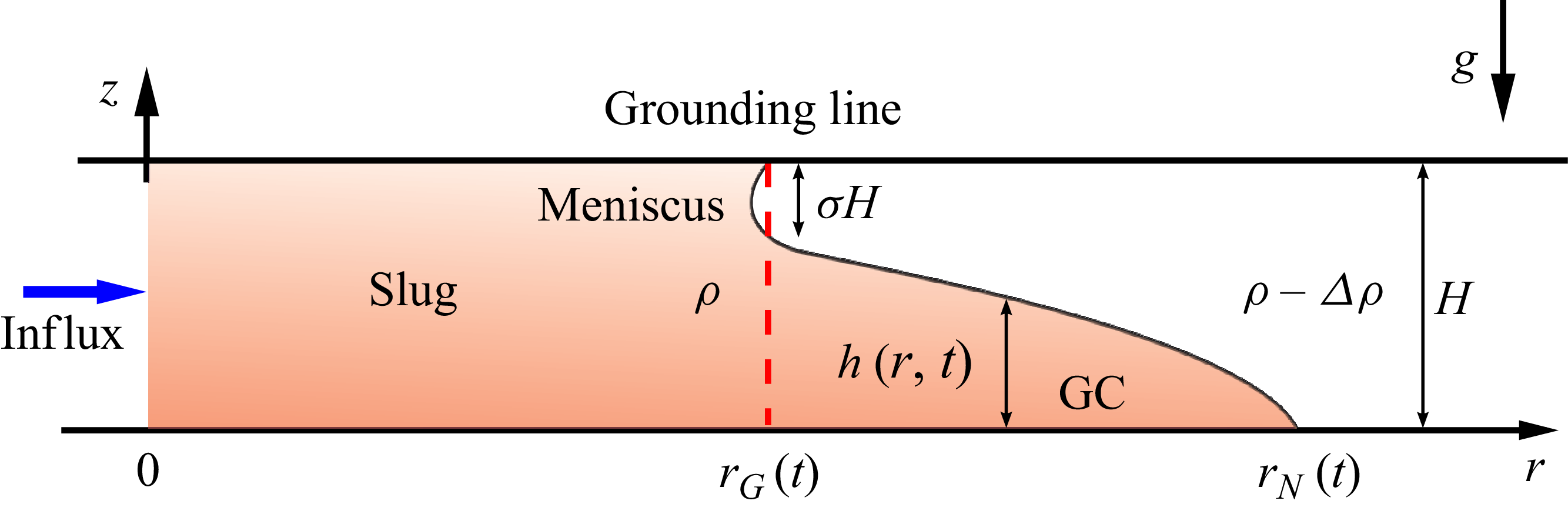
 σH
σH V=qtα
V=qtα rG=yGKtβ
 rN=Ktβ
 rG
rG J
J σ
σ α,β,K,yG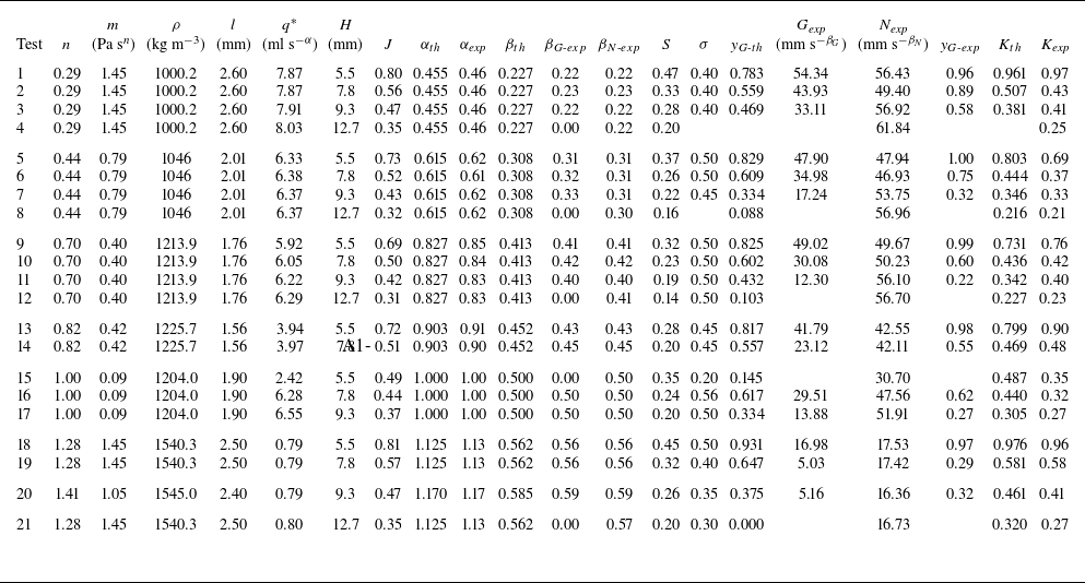
 n
n m
m ρ
ρ l=Γ/(ρg′)
 Γ
Γ ρg′
ρg′ q∗
q∗ α
α βG,N
βG,N S
S σ
σ yG=rG/rN
 Gexp
Gexp Nexp
Nexp K
K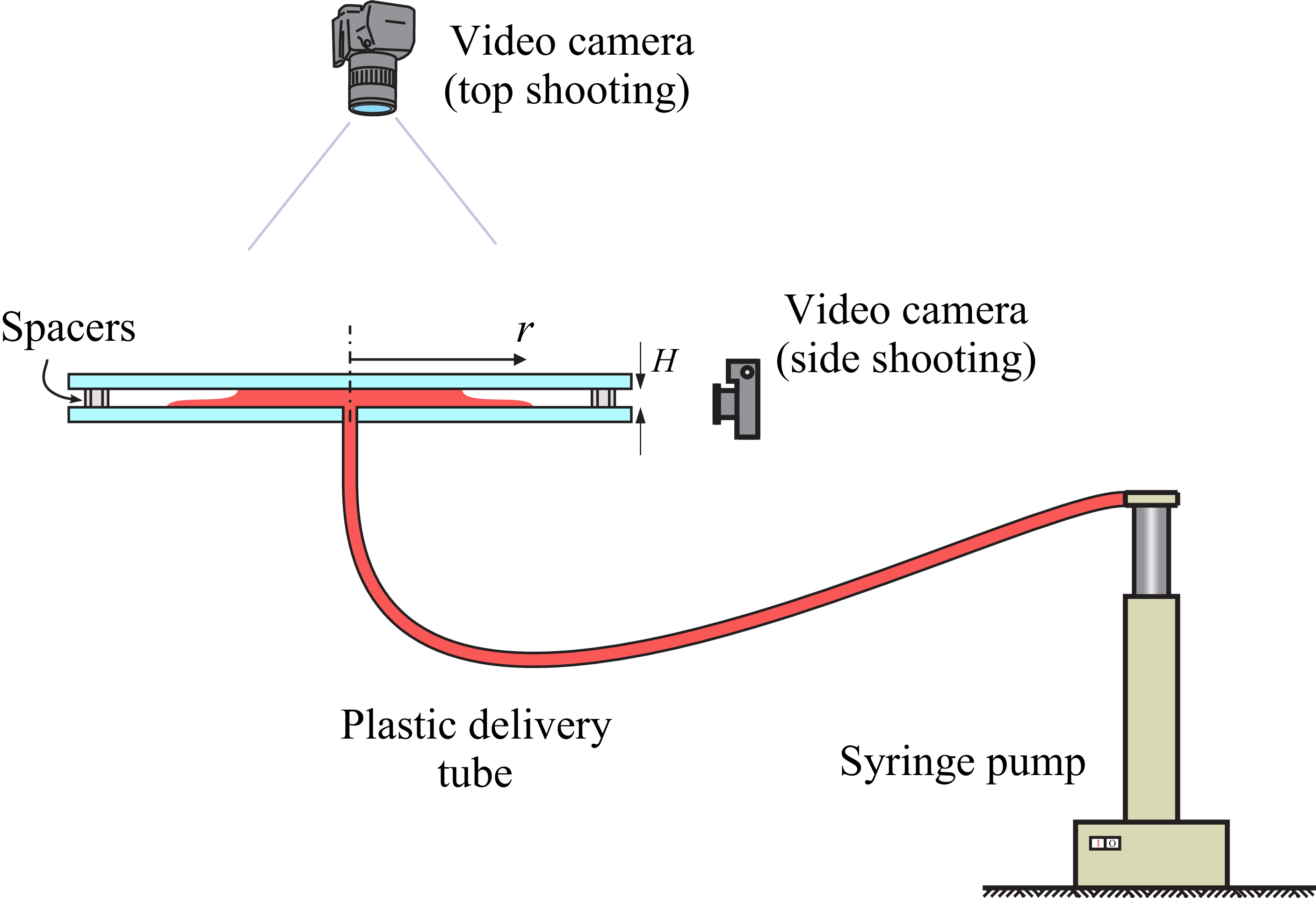
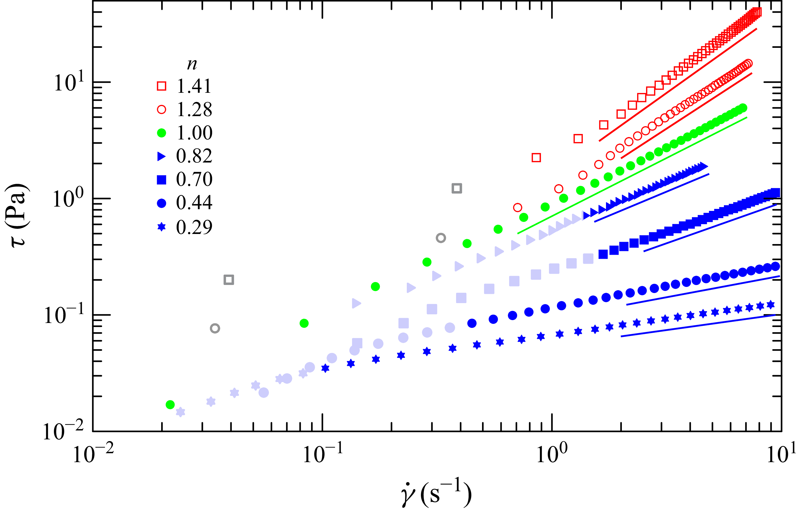
 γ˙
γ˙ τ
τ τ(γ˙)
τ(γ˙) τ=mγ˙n≡μγ˙
 n
n m
m
 t=32s
t=32s H=9.3mm
 n=0.29
 n=0.44
 n=0.70
 n=0.82,1
 n=1.28,1.41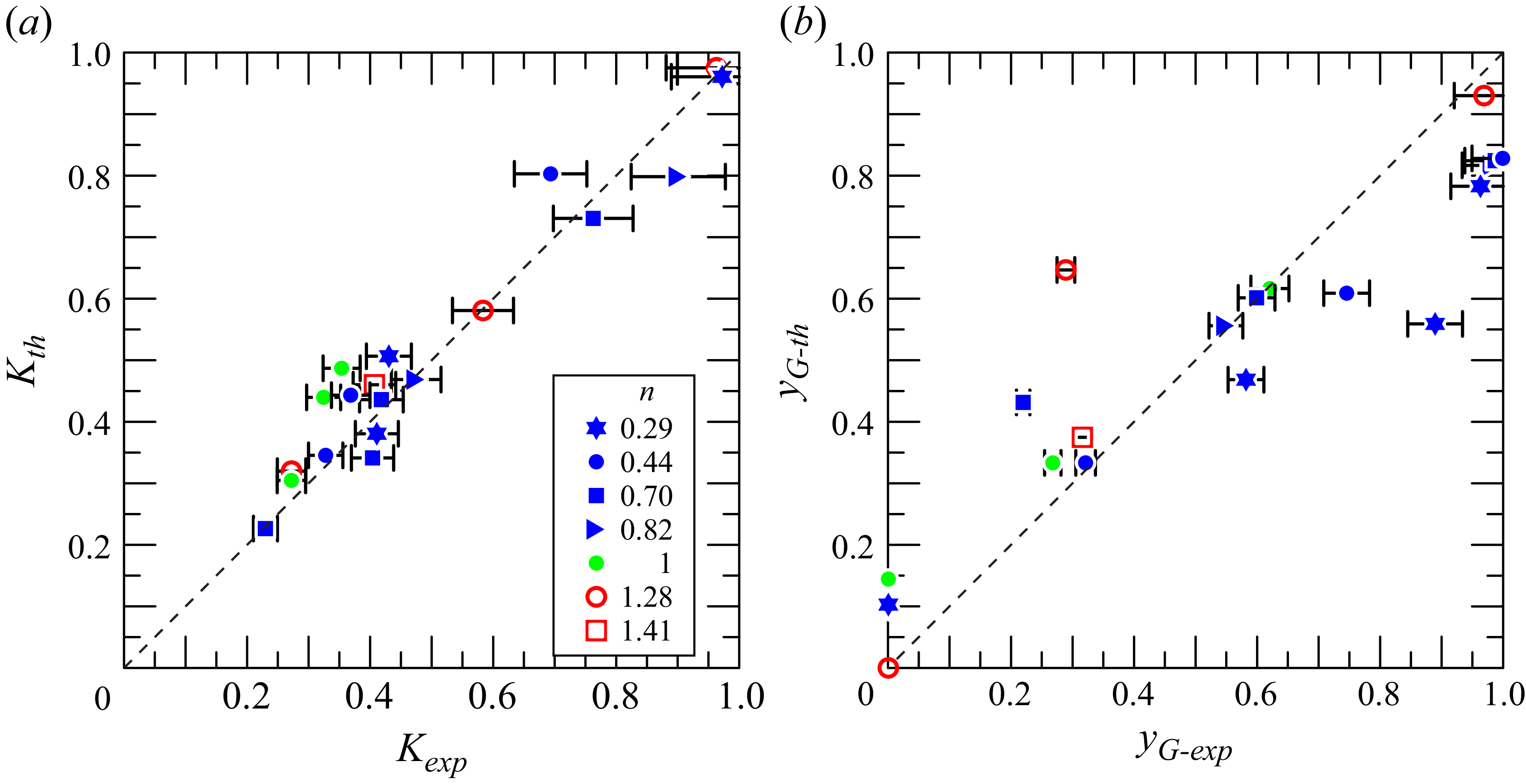
 K
K yG
yG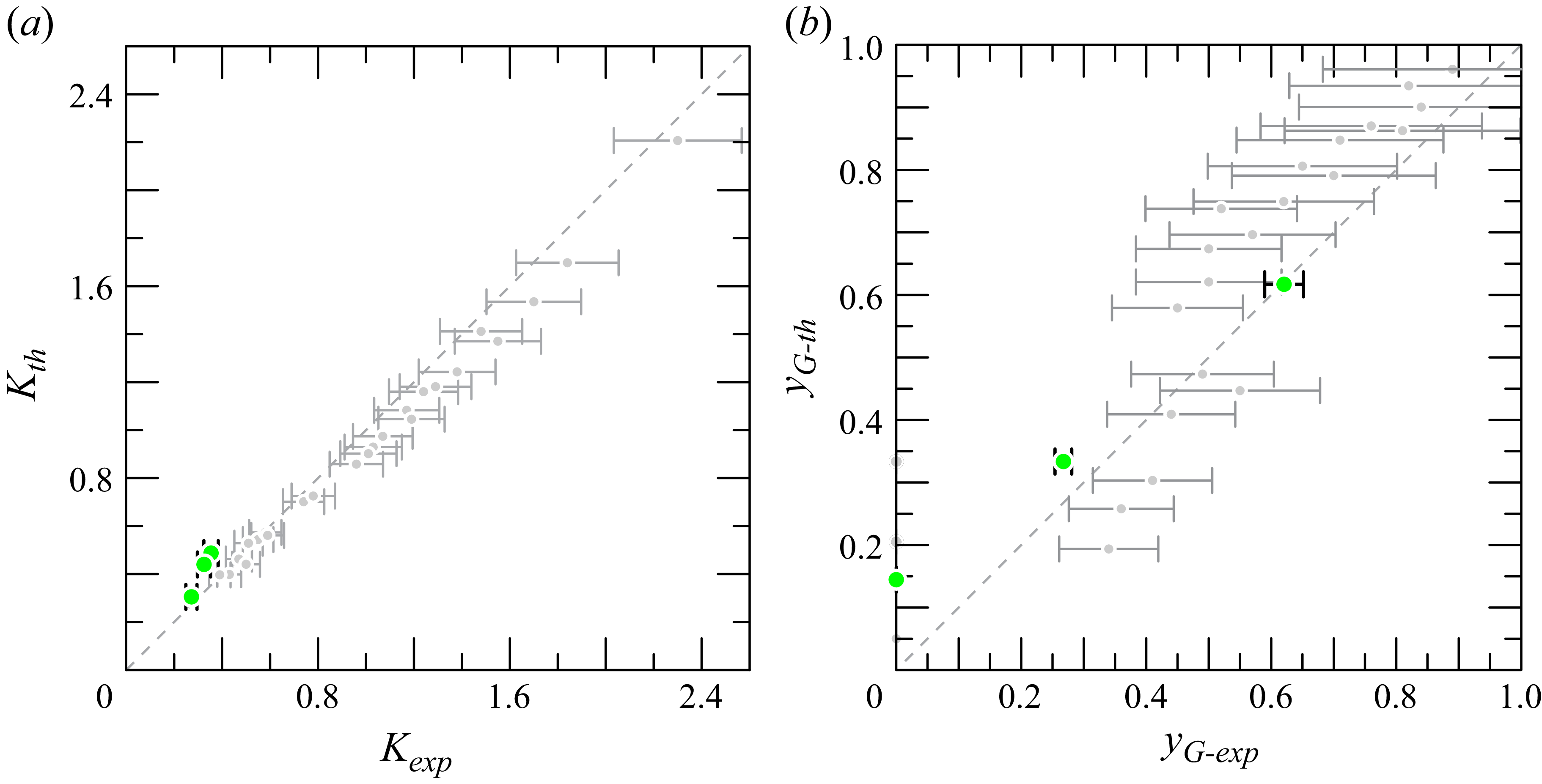
 K
K yG
yG
 J=0.47
 r0=1.25cm
 t0≈6
t0≈6
 H=9.3mm
 J=0.47
 Hn=9.25mm
 Hn=7.3mm
 Hn=6.3mm
 t=23s
t=23s
 γ˙N=r˙N/l
 γ˙r0=Q/(2πr0H2)


 Open access

