


1. Introduction
In recent years, machine learning has gained significant importance in fluid dynamics, and numerous studies have explored its application to address various challenges in this field (Duraisamy, Iaccarino & Xiao Reference Duraisamy, Iaccarino and Xiao2019; Brunton, Noack & Koumoutsakos Reference Brunton, Noack and Koumoutsakos2020; Zhang et al. Reference Zhang, Santoni, Herges, Sotiropoulos and Khosronejad2021; Vinuesa & Brunton Reference Vinuesa and Brunton2022; Zhang et al. 2023b). One area of its application is turbulence modelling, which includes both Reynolds-averaged Navier–Stokes (RANS) and large eddy simulation (LES). In the context of RANS, machine learning has been utilised to improve Reynolds stress closure modelling (Ling, Kurzawski & Templeton Reference Ling, Kurzawski and Templeton2016; Jiang et al. Reference Jiang, Vinuesa, Chen, Mi, Laima and Li2021; Sun et al. Reference Sun, Cao, Liu, Zhu and Zhang2022b ). For LES, it has been applied to enhance subgrid-scale (SGS) modelling (Gamahara & Hattori Reference Gamahara and Hattori2017; Wang et al. Reference Wang, Luo, Li, Tan and Fan2018b ; Zhou et al. Reference Zhou, He, Wang and Jin2019; Park & Choi Reference Park and Choi2021; Tabe Jamaat & Hattori Reference Tabe Jamaat and Hattori2022; Zhao, Jin & Zhou Reference Zhao, Jin and Zhou2022; Liu et al. Reference Liu, Yu, Huang, Liu and Lu2022) as well as wall modelling (Yang et al. Reference Yang, Zafar, Wang and Xiao2019; Bae & Koumoutsakos Reference Bae and Koumoutsakos2022; Tabe Jamaat & Hattori Reference Tabe Jamaat and Hattori2023; Lozano-Durán & Bae Reference Lozano-Durán and Bae2023; Tabe Jamaat et al. Reference Tabe Jamaat, Hattori and Kawai2024; Maejima, Tanino & Kawai Reference Maejima, Tanino and Kawai2024). Additionally, machine learning techniques have been employed for predicting complex turbulent flows in engineering and geophysical applications (Frank, Drikakis & Charissis Reference Frank, Drikakis and Charissis2020; Zhang et al. Reference Zhang, Flora, Kang, Limaye and Khosronejad2022; Chen et al. Reference Chen, Han, Wang, Zhao, Yang and Yang2023; Zhang et al. Reference Zhang, Sotiropoulos and Khosronejad2024a,b), flow field reconstruction (Fan et al. Reference Fan, Duan, Huang, Zhang and Yang2023; Yousif et al. Reference Yousif, Yu, Hoyas, Vinuesa and Lim2023; Matsuo et al. Reference Matsuo, Fukami, Nakamura, Morimoto and Fukagata2024; Fan et al. Reference Fan, Cheng, de, Audrey and Arcucci2025a ), flow control (Guastoni et al. Reference Guastoni, Rabault, Schlatter, Azizpour and Vinuesa2023; Vignon, Rabault & Vinuesa Reference Vignon, Rabault and Vinuesa2023; Ishize, Omichi & Fukagata Reference Ishize, Omichi and Fukagata2024) and solving partial differential equations (PDEs) for flow simulation (Li et al. Reference Li, Shu and Barati Farimani2023; McCabe et al. Reference McCabe2024; Rahman et al. Reference Rahman2024; Fan et al. Reference Fan, Akhare and Wang2025b ).
Another important application of machine learning in fluid dynamics is super-resolution (SR) reconstruction of flow fields, which has gained significant attention in recent years and was first introduced by Xie et al. (Reference Xie, Franz, Chu and Thuerey2018) and Fukami, Fukagata & Taira (Reference Fukami, Fukagata and Taira2019). Single-image SR is a fundamental low-level vision task that focuses on generating a high-resolution (HR) image from a low-resolution (LR) input while preserving structural and perceptual consistency. This task is challenging because it is an inverse problem, where a single LR image can correspond to multiple possible HR outputs.
Super-resolution techniques are recognised as effective tools for enhancing turbulent flow resolution, enabling more accurate predictions at lower computational costs. Direct numerical simulation (DNS), which is an HR simulation, resolves all flow scales but is computationally expensive, limiting its practical use. As a solution to these computational limitations, SR techniques can be employed to reconstruct fine-scale turbulence structures from coarse data while preserving the essential flow dynamics. These approaches can enhance the efficiency of numerical simulations and experimental measurements, bridging the gap between LR and HR data, and offer considerable potential for advancing turbulence research and its applications in engineering and industry.
The simplest SR method is interpolation, which fills in missing details using nearby data. It assumes smooth transitions, making it ineffective for capturing the chaotic and multi-scale nature of turbulence. In image SR, regression-based methods (Dong et al. Reference Dong, Loy, He and Tang2015; Liang et al. Reference Liang, Cao, Sun, Zhang, Van and Timofte2021; Sun et al. Reference Sun, Pan and Tang2022a ) like the convolutional neural network (CNN) establish a direct mapping from LR to HR images using a loss function, typically the mean squared error (MSE). However, these approaches tend to produce outputs with overly smoothed features, failing to capture fine details effectively (Gao et al. 2023), especially as the upsampling factor increases.
Deep generative models, such as autoregressive models (Chen et al. Reference Chen, Mishra, Rohaninejad and Abbeel2018; Lee et al. Reference Lee, Kim, Kim, Cho and Han2022), variational autoencoders (VAE) (Kingma & Welling Reference Kingma and Welling2013; Van Den Oord et al. Reference Van Den Oord2017) and the generative adversarial network (GAN) (Goodfellow et al. Reference Goodfellow, Pouget-Abadie, Mirza, Xu, Warde-Farley, Ozair, Courville and Bengio2014), have achieved notable success in generating high-quality images by learning the intricate distributions of images. These models have also been applied to the image SR task (Ledig et al. 2017; Liu et al. Reference Liu, Siu and Wang2021b ; Chira et al. Reference Chira, Haralampiev, Winther, Dittadi and Liévin2022; Guo et al. Reference Guo, Zhang, Wu, Wang, Zhang and Wang2022) to enhance fine details. However, GAN-based methods for SR often encounter issues like mode collapse, where the model generates a narrow range of similar outputs with limited diversity. Moreover, the training process is generally unstable and can take a long time to converge. To stabilise training, an additional discriminator is used, which is crucial for optimisation but unnecessary during inference, adding complexity to the model without providing direct benefits during testing (Isola et al. Reference Isola, Zhu, Zhou and Efros2017). On the other hand, VAE models underperform compared with GAN-based models, and autoregressive models are computationally expensive, limiting their application to LR images (Gao et al. Reference Gao, Liu, Zeng, Xu, Li, Luo, Liu, Zhen and Zhang2023).
There have been numerous studies on developing data-driven models for SR reconstruction of turbulent flows. Fukami, Fukagata & Taira (Reference Fukami, Fukagata and Taira2021) developed a CNN-based spatio-temporal SR model and applied it to spatio-temporal data for enhanced turbulent flow field reconstruction. Their results show that the model successfully reconstructs fine-scale turbulence structures, closely matching DNS results, and demonstrate the model’s ability to capture the key flow dynamics. However, their method struggles to reconstruct turbulent flow field in time when the temporal two-point correlation coefficient is low. Zhang et al. (2023a) developed a U-Net-based architecture (Ronneberger, Fischer & Brox Reference Ronneberger, Fischer and Brox2015) combined with additional convolutional layers for SR reconstruction of two-dimensional cylinder wake flow and hydrofoil velocity fields. They showed that their model outperforms both the standard U-Net and conventional CNN models. In a more recent study, Fukami & Taira (Reference Fukami and Taira2024) explored SR reconstruction using single snapshot data. They demonstrated that their approach can effectively recover HR turbulence structures, such as vortices and eddies, from limited input. They designed the test dataset to produce snapshots with vortical structures similar in size to those in subdomains of a single snapshot, which may limit the model’s ability to generalise to other flow structures. Additionally, since the model is CNN-based and the upsampling factor is high, the reconstructed flow field remains somewhat blurry.
In addition to CNN, the ability of transformer and GAN has been tested for SR reconstruction of turbulent flows. Xu et al. (Reference Xu, Zhuang, Pan and Wen2023) developed a transformer-based model (Chen et al. Reference Chen, Wang, Guo, Xu, Deng, Liu, Ma, Xu, XU and Gao2021a ) for SR reconstruction of turbulent channel flow and homogeneous isotropic turbulence (HIT). However, their model did not show significant improvement over CNN-based models, and they did not test it on data with an unseen Reynolds number to assess its generalisability to different flow conditions. Kim et al. (Reference Kim, Kim, Won and Lee2021) applied GAN (Ledig et al. 2017) and cycle-consistent GAN (CycleGAN) (Zhu et al. Reference Zhu, Park, Isola and Efros2017; Yuan et al. Reference Yuan, Liu, Zhang, Zhang, Dong and Lin2018), which are supervised and unsupervised learning approaches, respectively, to the SR reconstruction of HIT and turbulent channel flow. They showed that, for paired data, the GAN model results in lower error than the CycleGAN model. There are also other studies which have explored SR reconstruction of turbulent flows using CNN-based methods (Liu et al. Reference Liu, Tang, Huang and Lu2020; Zhou et al. Reference Zhou, Li, Yang and Yang2022), GAN-based approaches (Xie et al. Reference Xie, Franz, Chu and Thuerey2018; Yousif, Yu & Lim Reference Yousif, Yu and Lim2021; Chen et al. Reference Chen, Sammak, Givi, Yurko and Jia2021b ; Yousif, Yu & Lim Reference Yousif, Yu and Lim2022; Yu et al. Reference Yu, Yousif, Zhang, Hoyas, Vinuesa and Lim2022; Ward Reference Ward2023) and transformer-based methods (Tang et al. Reference Tang, Li, Zhao, Xiao and Chen2024; Zeng et al. Reference Zeng, Zhang, Xu and Feng2024; Liu et al. Reference Liu, Zhang, Guo, Li, Song and Yang2025). However, there is ongoing research to explore new deep learning methods for the SR reconstruction of turbulent flows and to develop a model with enhanced performance, capable of capturing flow structures of different sizes and applicable to various upsampling factors without producing a visually blurry flow field.
Recently, diffusion models have gained significant success in image generation (Ho, Jain & Abbeel Reference Ho, Jain and Abbeel2020; Dhariwal & Nichol Reference Dhariwal and Nichol2021), achieving state-of-the-art performance across various computer vision tasks. The iterative process of diffusion models has proven to be highly effective in learning complex distributions. These models have outperformed GANs, particularly excelling in generating high-quality, diverse and realistic images. Unlike GANs, which depend on adversarial training and often suffer from mode collapse, diffusion models employ a systematic process of transforming noise into the structured data through iterative denoising steps, resulting in more stable and higher-quality outputs. There are also several studies that have explored their application to image SR, demonstrating their effectiveness in enhancing image quality (Saharia et al. Reference Saharia, Ho, Chan, Salimans, Fleet and Norouzi2022; Li et al. Reference Li, Yang, Chang, Chen, Feng, Xu, Li and Chen2022; Gao et al. Reference Gao, Liu, Zeng, Xu, Li, Luo, Liu, Zhen and Zhang2023; Yue et al. Reference Yue, Wang and Loy2023).
Following their success in image generation, diffusion models have also been applied to the fluid dynamics field. Du et al. (Reference Du, Parikh, Fan, Liu and Wang2024) developed a framework based on the latent diffusion model (Rombach et al. Reference Rombach, Blattmann, Lorenz, Esser and Ommer2022) for generating spatio-temporal turbulence. They proposed a framework that combines a conditional neural field and a latent diffusion model to generate spatio-temporal turbulence. Their model effectively simulates complex turbulent flows across varying domains by conditioning the diffusion process on relevant spatio-temporal data. However, the model’s performance heavily depends on the size and diversity of the training data, requiring a sufficiently large set of subsequences to ensure effective generalisation. Shu, Li & Farimani (Reference Shu, Li and Farimani2023) used the denoising diffusion probabilistic model (DDPM) (Ho et al. Reference Ho, Jain and Abbeel2020; Saharia et al. Reference Saharia, Ho, Chan, Salimans, Fleet and Norouzi2022) with modifications for SR reconstruction of two-dimensional Kolmogorov flow and incorporated physics into their model by using the gradient of the PDE residual as conditioning information. The results of their study show that, compared with bicubic interpolation, the model can generate relatively high-quality flow fields without blurriness. However, it struggles to capture the flow details accurately, especially for the upsampling factor of 8. The obtained energy spectrum does not match the DNS results at high wavenumbers, indicating that the model has difficulty capturing the small-scale features of the flow. Additionally, the predicted vorticity distribution is less accurate than that produced by bicubic interpolation and deviates from the DNS results even for the upsampling factor of 4. Qi & Ma (Reference Qi and Ma2024) implemented the conditional denoising diffusion model (Saharia et al. Reference Saharia, Ho, Chan, Salimans, Fleet and Norouzi2022) to the SR reconstruction of turbulent flows. They found that, although the model learns the distribution, it does not achieve sufficient accuracy. To address this issue, they incorporated a residual network (He et al. Reference He, Zhang, Ren and Sun2016) to further improve the model’s performance. They tested their model on flow data with the same Reynolds number as that used in the training process, and showed that their model requires significantly more time for reconstruction compared with the CNN- and GAN-based models.
Despite their widespread use, diffusion models suffer from slow inference since they require hundreds or even thousands of sampling steps. Although accelerated sampling techniques can speed up computation, they often compromise performance, producing overly blurred SR results. In the present study, we aim to develop a data-driven model inspired by the strategy of the recently proposed ResShift diffusion model (Yue et al. Reference Yue, Wang and Loy2023) for the SR reconstruction of three-dimensional HIT, which can capture flow details well and generate clear HR flow fields without blurriness, even for high upsampling factors. Unlike the diffusion models used in previous studies on SR reconstruction of turbulent flows, the developed model has low inference time while being capable of generating HR flow fields. The ResShift model was originally developed for HR real-world and synthetic image reconstruction for the upsampling factor of 4, and has been applied, with some modifications, to the SR of microscopy images (Gao et al. Reference Gao, Gong, Cao, Wang, Zhang, Dong and Qiu2025) as well. Handling high compression rates in latent diffusion models (LDMs) is a significant challenge, as such rates can affect detail consistency and may lead to quality degradation during image reconstruction, especially as the compression rate increases (Lin et al. Reference Lin, Li, Hsiao, Ho and Kong2023). Additionally, because LDMs typically require an autoencoder tailored to a specific upsampling factor, using a pixel-wise formulation makes the model more flexible and easier to train without such constraints. Therefore, since capturing details is crucial for the SR of turbulent flows and we aim to train the model for different upsampling factors, unlike the original ResShift model, we construct the model in pixel space rather than latent space. Additionally, we include the perceptual loss in the training process to enhance the reconstruction quality and preserve fine flow structures.
In this study, we will use a large dataset obtained from the DNS of two HIT simulations with completely different parameters, including varying Reynolds numbers and grid sizes, to increase the generalisation ability of the model. We will also employ data from the whole domain as well as data from a quarter of the domain to increase the diversity of training samples, reduce the dependence of the model on domain-specific patterns and enable it to learn localised flow structures. The model will be trained for three SR ratios of 4, 8 and 16, and evaluated on data from the same simulations used for training as well as simulations with different parameters. The performance of the model will also be compared with that of bicubic interpolation, a CNN- and a U-Net-based model (Ronneberger et al. Reference Ronneberger, Fischer and Brox2015) and the conditional DDPM designed for SR Saharia et al. (Reference Saharia, Ho, Chan, Salimans, Fleet and Norouzi2022).
The paper is organised as follows. In § 2, we introduce the overall methodology, including the dataset details, the diffusion model description and the training set-up. The results of applying the diffusion model are presented and discussed in § 3, and the conclusions of the study are given in § 4.
2. Methodology
In the present study, we develop a diffusion model for the SR reconstruction of HIT. The model will be trained to predict the HR velocity components using the corresponding LR inputs. In this section, first, we provide the details of the dataset, which plays a crucial role in developing a reliable model. Next, we explain the diffusion model, which is used in this study for establishing an SR model for reconstructing the HR flow field. Finally, we present the training set-up, detailing the training process and hyperparameter choices.
2.1. Dataset preparation
To generate the training dataset, we conduct DNS for three-dimensional HIT. Direct numerical simulation was conducted using the same approach as Ishihara et al. (Reference Ishihara, Kaneda, Yokokawa, Itakura and Uno2007) and Miyazaki & Hattori (Reference Miyazaki and Hattori2020). We consider an incompressible fluid with a uniform density of one, governed by the Navier–Stokes (NS) equation
 \begin{align} \frac {\partial u_i}{\partial t}+\frac {\partial }{\partial x_j}({u_i}{u_{\kern-1pt j}})=-\frac {\partial p}{\partial x_i}+\nu \frac {\partial ^2 u_i}{\partial x_k x_k}+f, \end{align}
and continuity equation
 \begin{align} \frac {\partial u_i}{\partial x_i}=0, \end{align}
where $u$
,
$u$
, $p$
,
$p$
, $\nu$
and
$\nu$
and $f$
denote the velocity, pressure, kinematic viscosity and forcing term, respectively. The turbulence field is considered periodic in all directions of the Cartesian coordinate system, with a periodic domain of size
$f$
denote the velocity, pressure, kinematic viscosity and forcing term, respectively. The turbulence field is considered periodic in all directions of the Cartesian coordinate system, with a periodic domain of size $2\pi$
, allowing it to be represented as a Fourier series. The NS equations are solved using spectral method, and the dealiasing is performed by the phase-shift method, retaining Fourier modes satisfying
$2\pi$
, allowing it to be represented as a Fourier series. The NS equations are solved using spectral method, and the dealiasing is performed by the phase-shift method, retaining Fourier modes satisfying $k\lt k_{\textit{max}}=\sqrt {2}N/3$
, where
$k\lt k_{\textit{max}}=\sqrt {2}N/3$
, where $k$
and
$k$
and $N$
represent the wavenumber and number of grid points in each direction of the Cartesian coordinate system. The fourth-order Runge–Kutta method is used for time marching.
$N$
represent the wavenumber and number of grid points in each direction of the Cartesian coordinate system. The fourth-order Runge–Kutta method is used for time marching.
The forcing term $\hat {f}(k)=-c\hat {u}(k)$
is applied in wavenumber space, where
$\hat {f}(k)=-c\hat {u}(k)$
is applied in wavenumber space, where $\hat {f}$
and
$\hat {f}$
and $\hat {u}$
denote the Fourier transforms of
$\hat {u}$
denote the Fourier transforms of $f$
and
$f$
and $u$
, respectively. The coefficient
$u$
, respectively. The coefficient $c$
is non-zero only for wavenumbers within the range
$c$
is non-zero only for wavenumbers within the range $k\lt K_c=2.5$
and is dynamically adjusted at each time step to maintain the total kinematic energy
$k\lt K_c=2.5$
and is dynamically adjusted at each time step to maintain the total kinematic energy $E$
nearly constant (
$E$
nearly constant ( ${\approx}0.5$
). By restricting the forcing to lower wavenumbers, its direct influence on the small-scale dynamics is minimised. For the training dataset, we conduct two forced HIT simulations, HIT1 and HIT2, with different flow parameters, as shown in table 1, where
${\approx}0.5$
). By restricting the forcing to lower wavenumbers, its direct influence on the small-scale dynamics is minimised. For the training dataset, we conduct two forced HIT simulations, HIT1 and HIT2, with different flow parameters, as shown in table 1, where $ \textit{Re}_\lambda$
,
$ \textit{Re}_\lambda$
, $\Delta t$
,
$\Delta t$
, $\lambda$
,
$\lambda$
, $\eta$
,
$\eta$
, $\varepsilon$
and
$\varepsilon$
and $\mathcal{T}$
represent the Reynolds number based on the Taylor microscale, time-step size, Taylor microscale, Kolmogorov length scale, mean energy dissipation rate and the eddy turnover time, respectively.
$\mathcal{T}$
represent the Reynolds number based on the Taylor microscale, time-step size, Taylor microscale, Kolmogorov length scale, mean energy dissipation rate and the eddy turnover time, respectively.
Direct numerical simulation parameters and turbulence characteristics of HIT simulations.

In previous studies, various methods have been employed to obtain degraded LR data for the training process, including max and average pooling (Fukami et al. Reference Fukami, Fukagata and Taira2019; Kim et al. Reference Kim, Kim, Won and Lee2021), and selecting discrete points in the flow domain (Yu et al. Reference Yu, Yousif, Zhang, Hoyas, Vinuesa and Lim2022). In the present study, we apply the Gaussian filter to the DNS data, which can produce smooth and physically consistent coarse-grained flow fields. This method has been commonly used in data-driven turbulence modelling for LES as it helps make the data more representative of LES flow fields and has been shown to yield more accurate models than other filter types, such as sharp spectral and top-hat filters (Zhou et al. Reference Zhou, He, Wang and Jin2019; Miyazaki & Hattori Reference Miyazaki and Hattori2020; Tabe Jamaat & Hattori Reference Tabe Jamaat and Hattori2022). The Gaussian filter kernel is defined as
 \begin{align} \hat {G}(k)=\text{exp} \left(-\frac {k^2\Delta ^2}{24} \right)\!, \end{align}
in the spectral space, where $G$
and
$G$
and $\Delta$
denote the filter kernel and filter width, respectively. After applying the Gaussian filter, we coarse grain the results to the desired number of grid points in the LR flow field (Zanna & Bolton Reference Zanna and Bolton2020; Guan et al. Reference Guan, Chattopadhyay, Subel and Hassanzadeh2022). The coarse graining is performed in spectral space as well by applying a cutoff filter to the data
$\Delta$
denote the filter kernel and filter width, respectively. After applying the Gaussian filter, we coarse grain the results to the desired number of grid points in the LR flow field (Zanna & Bolton Reference Zanna and Bolton2020; Guan et al. Reference Guan, Chattopadhyay, Subel and Hassanzadeh2022). The coarse graining is performed in spectral space as well by applying a cutoff filter to the data
 \begin{align} \hat {G} = H(k_c - |k|) , \end{align}
where $k_c=\pi /\Delta$
is the cutoff wavenumber and
$k_c=\pi /\Delta$
is the cutoff wavenumber and $H$
denotes the Heaviside step function. The filter size
$H$
denotes the Heaviside step function. The filter size $\Delta$
is determined based on the upsampling factor. For instance, when
$\Delta$
is determined based on the upsampling factor. For instance, when $N=256$
and the upsampling factor is 4,
$N=256$
and the upsampling factor is 4, $\Delta = 2\pi /64$
, where 64 corresponds to the number of grid points in the LR flow field.
$\Delta = 2\pi /64$
, where 64 corresponds to the number of grid points in the LR flow field.
There have been different methods used for normalising the training dataset. In the studies by Yousif et al. (Reference Yousif, Yu and Lim2021), Tang et al. (Reference Tang, Li, Zhao, Xiao and Chen2024) and Yu et al. (Reference Yu, Yousif, Zhang, Hoyas, Vinuesa and Lim2022), the data are non-dimensionalised using min–max normalisation. However, in a study by Fukami & Taira (Reference Fukami and Taira2024) on the SR reconstruction of two-dimensional decaying isotropic turbulence, the input and output data are normalised using the instantaneous maximum absolute vorticity to consider the magnitude variations in the vorticity field at different Reynolds numbers. In the present study, we normalise the data of each velocity component using the maximum absolute value of the corresponding velocity component. Our training dataset includes 25 600 snapshots, each of size $256^2$
, which is considerably larger than the datasets used in the previous studies (Liu et al. Reference Liu, Tang, Huang and Lu2020; Xu et al. Reference Xu, Zhuang, Pan and Wen2023), and the validation dataset includes 800 snapshots. In more detail, for training, 800 time steps with a uniform time interval of 0.2 are selected for HIT1, and 200 time steps with a uniform time interval of 0.1 are chosen for HIT2. For the validation dataset, 10 time steps are uniformly selected for both HIT1 and HIT2, with time intervals of 2 and 1, respectively. In each time step, 16
$256^2$
, which is considerably larger than the datasets used in the previous studies (Liu et al. Reference Liu, Tang, Huang and Lu2020; Xu et al. Reference Xu, Zhuang, Pan and Wen2023), and the validation dataset includes 800 snapshots. In more detail, for training, 800 time steps with a uniform time interval of 0.2 are selected for HIT1, and 200 time steps with a uniform time interval of 0.1 are chosen for HIT2. For the validation dataset, 10 time steps are uniformly selected for both HIT1 and HIT2, with time intervals of 2 and 1, respectively. In each time step, 16 $x$
–
$x$
– $y$
planes are extracted. We have also evaluated the impact of training data size by comparing the model trained with the original dataset to one trained with twice the dataset size, ensuring sufficient data for the training process.
$y$
planes are extracted. We have also evaluated the impact of training data size by comparing the model trained with the original dataset to one trained with twice the dataset size, ensuring sufficient data for the training process.
For data from the simulation on the grid size of $512^3$
(HIT2), we divide each two-dimensional snapshot into four subdomains, each of size
$512^3$
(HIT2), we divide each two-dimensional snapshot into four subdomains, each of size $256^2$
. This form of data augmentation increases both the diversity and number of training samples. Furthermore, it reduces the model’s reliance on global, domain-specific patterns and enhances its ability to learn localised flow structures, which is beneficial for reconstructing turbulent features at high upsampling factors. This choice of domain size for HIT2 satisfies the condition that the domain length should be larger than the integral length scale.
$256^2$
. This form of data augmentation increases both the diversity and number of training samples. Furthermore, it reduces the model’s reliance on global, domain-specific patterns and enhances its ability to learn localised flow structures, which is beneficial for reconstructing turbulent features at high upsampling factors. This choice of domain size for HIT2 satisfies the condition that the domain length should be larger than the integral length scale.
Since the training data come from different simulations and the dataset size is large, the model is expected to generalise reasonably well to flow fields with varying Reynolds numbers and grid sizes. The data-driven SR model will be trained for three upsampling factors of 4, 8 and 16. In all cases, the output size will be fixed, and the input sizes will be 64, 32 and 16, respectively. In Appendix A, additional details have been provided on the relationship between the LR grid spacing and the characteristic turbulence scales.
For evaluation, the model is tested on data from simulations with Reynolds numbers lower and higher than those of the training data. Furthermore, the model will be tested on input sizes significantly larger than those of the training data. The test dataset includes data from two different simulations, as well as data from the same simulations used for training but at different time steps. The simulation settings for the test cases are similar to those of the training data, with grid sizes and viscosities set to $256^3$
and
$256^3$
and $5\times 10^{-3}$
for the lower Reynolds number flow, and
$5\times 10^{-3}$
for the lower Reynolds number flow, and $1024^3$
and
$1024^3$
and $2.8\times 10^{-4}$
for the higher Reynolds number flow. The details of the simulations for the test cases HIT3 and HIT4 are provided in table 1. In Appendix B, we also test the model on the LR data obtained using average pooling to assess the model’s sensitivity to the coarse-graining method.
$2.8\times 10^{-4}$
for the higher Reynolds number flow. The details of the simulations for the test cases HIT3 and HIT4 are provided in table 1. In Appendix B, we also test the model on the LR data obtained using average pooling to assess the model’s sensitivity to the coarse-graining method.
2.2. Diffusion model for SR reconstruction
In this study, we develop a diffusion model based on the ResShift model (Yue et al. Reference Yue, Wang and Loy2023) for SR reconstruction of HIT. The model employs a Markov chain to transfer between HR and LR data by shifting the residuals between them, greatly improving the transition efficiency. A detailed noise schedule also manages the shifting speed and noise strength during the diffusion process. Unlike the original ResShift model, which was developed for image SR in latent space at a fixed upsampling ratio, the present model operates in pixel space on turbulent flow fields, enabling easy applicability to different upsampling factors (4, 8, 16) and improving pixel-wise accuracy. As will be discussed later, perceptual loss is incorporated to better capture fine-scale vortical structures, and a cosine learning rate scheduler enhances training stability and generalisation. These modifications allow more accurate reconstruction of multi-scale turbulence while preserving high-frequency details.
Schematic of ResShift diffusion model.

In the SR task using diffusion models, one common approach is to input the LR image into the model and retrain it from scratch using the training data. Alternatively, an unconditional pretrained diffusion model can be used as a prior, adjusting the reverse path to generate the HR image. However, both approaches often suffer from inefficiencies during inference, requiring hundreds or even thousands of sampling steps (Ho et al. Reference Ho, Jain and Abbeel2020; Saharia et al. Reference Saharia, Ho, Chan, Salimans, Fleet and Norouzi2022). Furthermore, existing acceleration techniques aimed at speeding up inference and the sampling process usually compromise performance, leading to over-smoothed results (Song, Meng & Ermon Reference Song, Meng and Ermon2020; Nichol & Dhariwal Reference Nichol and Dhariwal2021). The strategy used in the ResShift diffusion model addresses both efficiency and performance. Diffusion models generally consist of two main stages: the forward process and the backward process. In this section, we outline these stages within the context of the ResShift model, which is focused on the SR task. A schematic of the ResShift diffusion model is shown in figure 1.
The ResShift model facilitates the transition from an HR image ( $x_0$
) to an LR image (
$x_0$
) to an LR image ( $y$
) by gradually shifting the residual, defined as
$y$
) by gradually shifting the residual, defined as $d=y-x_0$
, through a Markov chain over
$d=y-x_0$
, through a Markov chain over $T$
steps.
$T$
steps. $T$
is set to 15, which is significantly lower than that of other diffusion models (Ho et al. Reference Ho, Jain and Abbeel2020; Song et al. Reference Song, Meng and Ermon2020; Rombach et al. Reference Rombach, Blattmann, Lorenz, Esser and Ommer2022), leading to a notable reduction in the computational cost of inference. To ensure both images share the same spatial resolution, the LR image
$T$
is set to 15, which is significantly lower than that of other diffusion models (Ho et al. Reference Ho, Jain and Abbeel2020; Song et al. Reference Song, Meng and Ermon2020; Rombach et al. Reference Rombach, Blattmann, Lorenz, Esser and Ommer2022), leading to a notable reduction in the computational cost of inference. To ensure both images share the same spatial resolution, the LR image $y$
is first upsampled using bicubic interpolation. The Markov chain serves as a bridge between the HR and LR images, while the diffusion process integrates information from the LR image, enabling SR through reverse sampling conditioned on it. The shifting sequence
$y$
is first upsampled using bicubic interpolation. The Markov chain serves as a bridge between the HR and LR images, while the diffusion process integrates information from the LR image, enabling SR through reverse sampling conditioned on it. The shifting sequence $\{\eta _t\}_{t=1}^T$
increases monotonically with time step
$\{\eta _t\}_{t=1}^T$
increases monotonically with time step $t$
, satisfying
$t$
, satisfying $\eta _1 \to 0$
and
$\eta _1 \to 0$
and $\eta _T \to 1$
. In the forward process, the marginal distribution at any time step
$\eta _T \to 1$
. In the forward process, the marginal distribution at any time step $t \in \{1, 2, \ldots , T\}$
can be obtained as follows:
$t \in \{1, 2, \ldots , T\}$
can be obtained as follows:
 \begin{align} q(x_t|x_0,y)=\mathcal{N} \big(x_t;x_0+\eta _t d, k^2\eta _t I \big), \end{align}
where $k$
is a hyperparameter controlling the noise variance, which is set to 2,
$k$
is a hyperparameter controlling the noise variance, which is set to 2, $I$
is the identity matrix and
$I$
is the identity matrix and $\mathcal{N}(x_t; \mu _t, \sigma _t^2)$
denotes the Gaussian (normal) distribution over
$\mathcal{N}(x_t; \mu _t, \sigma _t^2)$
denotes the Gaussian (normal) distribution over $x_t$
with mean
$x_t$
with mean $\mu _t$
and variance
$\mu _t$
and variance $\sigma _t^2$
, which can be equivalently written as
$\sigma _t^2$
, which can be equivalently written as
 \begin{align} x_t = \mu _t + \sigma _t\epsilon , \quad \epsilon \sim \mathcal{N}(0, I), \end{align}
where $\mu _t=x_0+\eta _t d$
and
$\mu _t=x_0+\eta _t d$
and $\sigma _t^2=k^2\eta _t I$
. The schedule for
$\sigma _t^2=k^2\eta _t I$
. The schedule for $\eta _t$
is
$\eta _t$
is
 \begin{align} \sqrt {\eta _t} = \sqrt {\eta _1} \times b_0^{\beta _t}, \end{align}
where $t=\{2,\ldots ,T-1\}$
.
$t=\{2,\ldots ,T-1\}$
. $b_0$
is
$b_0$
is
 \begin{align} b_0 = \text{exp}\Big [\frac {1}{2(T-1)} \text{log}\frac {\eta _T}{\eta _1}\Big ], \end{align}
and $\beta _t$
is defined as
$\beta _t$
is defined as
 \begin{align} \beta _t=\Big (\frac {t-1}{T-1}\Big )^p \times (T-1), \end{align}
where $p=0.3$
.
$p=0.3$
.
The aim of the reverse process is to gradually denoise a noisy sample by reversing the forward diffusion process and estimating the posterior distribution $p(x_0|y)$
. The inverse process can be performed as follows:
$p(x_0|y)$
. The inverse process can be performed as follows:
 \begin{align} p_\theta (x_{t-1}|x_t,y)=\mathcal{N}(x_{t-1};\mu _\theta (x_t,y,t), k^2\frac {\eta _{t-1}}{\eta _t}\alpha _tI), \end{align}
where $\alpha _1 = \eta _1$
and
$\alpha _1 = \eta _1$
and $\alpha _t =\eta _t - \eta _{t-1}$
for
$\alpha _t =\eta _t - \eta _{t-1}$
for $t\gt 1$
. Therefore,
$t\gt 1$
. Therefore, $x_{t-1}$
can be calculated as follows:
$x_{t-1}$
can be calculated as follows:
 \begin{align} x_{t-1} = \mu _\theta +\sigma _t\epsilon , \quad \epsilon \sim \mathcal{N}(0, I), \end{align}
where $\sigma _t^2= k^2 ({\eta _{t-1}}/{\eta _t})\alpha _t I$
. The mean parameter
$\sigma _t^2= k^2 ({\eta _{t-1}}/{\eta _t})\alpha _t I$
. The mean parameter $\mu _\theta$
is reparameterised as
$\mu _\theta$
is reparameterised as
 \begin{align} \mu _\theta (x_t,y,t)=\frac {\eta _{t-1}}{\eta _t} x_t + \frac {\alpha _t}{\eta _t} f_\theta (x_t, y,t), \end{align}
where $f_\theta$
is a deep network with trainable parameters (weights)
$f_\theta$
is a deep network with trainable parameters (weights) $\theta$
. The network
$\theta$
. The network $f_\theta$
is trained to predict
$f_\theta$
is trained to predict $x_0$
from the noisy intermediate state
$x_0$
from the noisy intermediate state $x_t$
, conditioned on the LR flow field (
$x_t$
, conditioned on the LR flow field ( $y$
) and the time step
$y$
) and the time step $t$
, by minimising the loss function between the predicted and ground truth
$t$
, by minimising the loss function between the predicted and ground truth $x_0$
. The reverse process starts from the final time step
$x_0$
. The reverse process starts from the final time step $T$
, and the model denoises step-by-step using the learned posterior
$T$
, and the model denoises step-by-step using the learned posterior $p_\theta$
, progressively reconstructing less noisy flow fields until the final HR flow field
$p_\theta$
, progressively reconstructing less noisy flow fields until the final HR flow field $x_0$
is obtained. The same network
$x_0$
is obtained. The same network $f_\theta$
is used for all steps during both training and inference, and since the forward schedule
$f_\theta$
is used for all steps during both training and inference, and since the forward schedule $\{\eta _t\}$
controls the noise level at each step, errors naturally vary with
$\{\eta _t\}$
controls the noise level at each step, errors naturally vary with $t$
.
$t$
.
2.3. Model training set-up
We utilise the Adam optimiser (Kingma & Ba Reference Kingma and Ba2014) with a cosine learning rate scheduler for smoother and improved convergence, where the minimum learning rate is set to $2\times 10^{-5}$
. The batch size is 64 and the training is performed for 500 epochs.
$2\times 10^{-5}$
. The batch size is 64 and the training is performed for 500 epochs.
Most previous studies on SR reconstruction of turbulent flows, particularly those employing CNN-based models, have relied solely on MSE as the loss function (Fukami et al. Reference Fukami, Fukagata and Taira2019, Reference Fukami, Fukagata and Taira2021; Xu et al. Reference Xu, Zhuang, Pan and Wen2023; Zhang et al. Reference Zhang, Liu and Huang2023a ). However, there have been some recent studies that employed perceptual loss (Johnson, Alahi & Fei-Fei Reference Johnson, Alahi and Fei-Fei2016; Ledig et al. 2017; Zhang et al. Reference Zhang, Isola, Efros, Shechtman and Wang2018) together with MSE (Yousif et al. Reference Yousif, Yu and Lim2021; Yu et al. Reference Yu, Yousif, Zhang, Hoyas, Vinuesa and Lim2022; Tang et al. Reference Tang, Li, Zhao, Xiao and Chen2024). The perceptual loss measures the difference in the extracted features between the ground truth and predicted data. It improves the perceptual quality of the reconstructed images by focusing on high-level features rather than pixel accuracy. By emphasising feature-level consistency, it helps preserve important structures and patterns, reduces artefacts and blurriness and improves the overall clarity and realism of the generated outputs.
To capture perceptual quality more effectively, we adopt the learned perceptual image patch similarity (LPIPS) loss, a perceptual loss based on deep feature distance. The LPIPS captures differences in learned representations, making it suitable for preserving complex spatial patterns in turbulent flows that pixel-wise losses may not capture well. We use the pretrained deep convolutional network VGG16 (Simonyan & Zisserman Reference Simonyan and Zisserman2014) to extract features. A schematic of VGG16 and its feature extraction process in different layers is shown in figure 2. The three velocity components are used as the input channels to VGG16. While the study by Wang et al. (Reference Wang, Yu, Wu, Gu, Liu, Dong, Qiao and Change Loy2018a ) used only a single layer of VGG19 for feature extraction, subsequent research (Yousif et al. Reference Yousif, Yu and Lim2021) has shown that leveraging more layers can improve training stability. Therefore, we employ five layers from VGG16 to extract multi-scale features. The features in different blocks are extracted at the end of each block, just before the pooling layer.
In this study, the objective function is the combination of reconstruction loss $L_{\textit{MSE}}$
, which is the MSE, and the perceptual loss
$L_{\textit{MSE}}$
, which is the MSE, and the perceptual loss $L_p$
$L_p$
 \begin{align} L_{\textit{tot}}=L_{\textit{MSE}}+\lambda L_{p}, \end{align}
A schematic of the VGG16 network.

where $\lambda$
is set to 0.005 and
$\lambda$
is set to 0.005 and $L_{\textit{MSE}}$
is defined as
$L_{\textit{MSE}}$
is defined as
 \begin{align} L_{\textit{MSE}} = \frac {1}{N} \sum _{j=1}^{N} \| \hat {u}_j - u_{\kern-1pt j} \|_2^2, \end{align}
where $\hat {u}_j$
is the predicted velocity for the
$\hat {u}_j$
is the predicted velocity for the ${j}$
th data point,
${j}$
th data point, $u_{\kern-1pt j}$
is the corresponding ground truth velocity and
$u_{\kern-1pt j}$
is the corresponding ground truth velocity and $N$
is the total number of data points in the batch. Also,
$N$
is the total number of data points in the batch. Also, $L_p$
is given by
$L_p$
is given by
 \begin{align} L_{p}= \sum _{l=1}^{L}w_l||\phi _l(\hat {u}_j)-\phi _l(u_{\kern-1pt j})||_2^2, \end{align}
where $\phi _l$
represents the feature map at the
$\phi _l$
represents the feature map at the $l_{\text{}}$
th layer of the pretrained network, which is VGG16 in this study,
$l_{\text{}}$
th layer of the pretrained network, which is VGG16 in this study, $w_l$
is the learned weight of the
$w_l$
is the learned weight of the $l_{\text{}}$
th layer and
$l_{\text{}}$
th layer and $L$
denotes the layers used for the loss calculation. A schematic of LPIPS loss calculation is shown in figure 3.
$L$
denotes the layers used for the loss calculation. A schematic of LPIPS loss calculation is shown in figure 3.
To predict the HR flow field ( $x_0$
) using
$x_0$
) using $f_\theta$
in (2.12), the U-Net model (Ronneberger et al. Reference Ronneberger, Fischer and Brox2015) is used. A schematic of the U-Net model is presented in figure 4. The U-Net architecture used in DDPM (Ho et al. Reference Ho, Jain and Abbeel2020), combined with the Swin transformer (Liu et al. Reference Liu, Lin, Cao, Hu, Wei, Zhang, Lin and Guo2021a
) block instead of the self-attention layer, is employed as the deep network to improve the model’s performance.
$f_\theta$
in (2.12), the U-Net model (Ronneberger et al. Reference Ronneberger, Fischer and Brox2015) is used. A schematic of the U-Net model is presented in figure 4. The U-Net architecture used in DDPM (Ho et al. Reference Ho, Jain and Abbeel2020), combined with the Swin transformer (Liu et al. Reference Liu, Lin, Cao, Hu, Wei, Zhang, Lin and Guo2021a
) block instead of the self-attention layer, is employed as the deep network to improve the model’s performance.
The hierarchical structure and shifted window mechanism of the Swin transformer enable effective modelling of local and global dependencies while allowing the network to handle input sizes. Attention is computed within local windows and gradually aggregated across shifted windows, providing flexibility for various input resolutions (Liu et al. Reference Liu, Lin, Cao, Hu, Wei, Zhang, Lin and Guo2021a ). Combined with the convolutional blocks, which are inherently resolution agnostic, the network can accommodate different input sizes without retraining. Since we evaluate the model across different resolutions, this design can enhance the robustness and adaptability of the model to various input sizes. The details of the U-Net architecture are presented in Appendix C. Additionally, in Appendix D, the advantages of using pixel-wise diffusion model, the LPIPS loss and the Swin transformer are further discussed.
Illustration of LPIPS loss function computation process.

A schematic of U-Net.

3. Results
In this section, the trained diffusion model is assessed on various cases, including data from the same simulations used in the training process at time steps different from those of the training data, and data from two other simulations, HIT3 and HIT4, as presented in table 1. The ability of the diffusion model in predicting the HR flow field is evaluated for three upsampling factors of 4, 8 and 16.
We will also compare the performance of the diffusion model presented in this study with bicubic interpolation, a CNN model, a U-Net-based model and the conditional DDPM designed for SR (Saharia et al. Reference Saharia, Ho, Chan, Salimans, Fleet and Norouzi2022) to investigate the improvements achieved by using the developed diffusion model. The diffusion model presented in this study and the conditional DDPM (Saharia et al. Reference Saharia, Ho, Chan, Salimans, Fleet and Norouzi2022) are referred to as residual-based diffusion model (DM) and DDPM in this study, respectively. The CNN model we use for comparison includes only convolutional layers with the kernel size of $3 \times 3$
and upsampling layers, with leaky rectified linear unit (LReLU) as the activation function. A schematic of the CNN model used in the present study is shown in figure 5. The U-Net architecture used for comparison in this study is adapted from the original U-Net model (Ronneberger et al. Reference Ronneberger, Fischer and Brox2015) for the SR task with some modifications. It takes three-channel inputs and outputs, where the inputs correspond to bicubic-interpolated LR flow fields and the outputs are HR flow fields. Downsampling is performed using average pooling, while upsampling is achieved through bicubic interpolation to ensure smoother reconstruction and improved preservation of flow structures.
$3 \times 3$
and upsampling layers, with leaky rectified linear unit (LReLU) as the activation function. A schematic of the CNN model used in the present study is shown in figure 5. The U-Net architecture used for comparison in this study is adapted from the original U-Net model (Ronneberger et al. Reference Ronneberger, Fischer and Brox2015) for the SR task with some modifications. It takes three-channel inputs and outputs, where the inputs correspond to bicubic-interpolated LR flow fields and the outputs are HR flow fields. Downsampling is performed using average pooling, while upsampling is achieved through bicubic interpolation to ensure smoother reconstruction and improved preservation of flow structures.
A schematic of the CNN model architecture for the upsampling factor of 8. Here, CL denotes a convolutional layer.

3.1. Qualitative analysis of reconstructed HR flow fields
The velocity distribution for HIT2 is presented in figure 6. In this case, the input size is $512^2$
, which differs from the input size of
$512^2$
, which differs from the input size of $256^2$
used during the training process. As seen in figure 6, all models are able to predict the flow field roughly well for the upsampling factor of 4. As the upsampling factor increases, bicubic interpolation and the CNN model generate blurry HR reconstructions and fail to capture the small-scale flow structures. The DDPM tends to underpredict or overpredict the flow field for all upsampling factors. This issue with DDPM has been observed in the previous study by Qi & Ma (Reference Qi and Ma2024) as well. The U-Net model shows better performance than bicubic interpolation and the CNN model although it also predicts almost a blurry flow field for the upsampling factor of 16. However, the residual-based DM can generate a clear HR flow field with no blurriness, capable of capturing small-scale features, even at high upsampling factors.
$256^2$
used during the training process. As seen in figure 6, all models are able to predict the flow field roughly well for the upsampling factor of 4. As the upsampling factor increases, bicubic interpolation and the CNN model generate blurry HR reconstructions and fail to capture the small-scale flow structures. The DDPM tends to underpredict or overpredict the flow field for all upsampling factors. This issue with DDPM has been observed in the previous study by Qi & Ma (Reference Qi and Ma2024) as well. The U-Net model shows better performance than bicubic interpolation and the CNN model although it also predicts almost a blurry flow field for the upsampling factor of 16. However, the residual-based DM can generate a clear HR flow field with no blurriness, capable of capturing small-scale features, even at high upsampling factors.
Reconstructed instantaneous velocity field ( $u$
) from the LR input for HIT2. Here, DM and GT denote the residual-based diffusion model and ground truth (DNS), respectively.
$u$
) from the LR input for HIT2. Here, DM and GT denote the residual-based diffusion model and ground truth (DNS), respectively.

To further investigate the performance of the model, it is tested on two additional cases, HIT3 and HIT4. As seen in table 1, the viscosities in HIT3 and HIT4 are significantly smaller and larger, respectively, compared with those of the training data, making them challenging for the model and providing a rigorous test of its generalisation capability. The velocity distribution of HIT3 at the upsampling factor of 8 is presented in figure 7. As seen in this figure, although HIT3 differs from the training data, it is not difficult for the models to achieve reasonable accuracy in predicting the velocity field. In fact, due to its lower Reynolds number, there are fewer complex, chaotic structures compared with the higher Reynolds number case, HIT2, and it exhibits smoother, more predictable behaviour. This makes it easier for the models to capture and upscale the flow field without blurriness. Nevertheless, even in this case, the velocity predictions by bicubic interpolation, the CNN and the U-Net models is over-smoothed, and the residual-based DM achieves a slightly better prediction.
Reconstructed instantaneous velocity field ( $u$
) from the LR input for HIT3 (upsampling factor = 8). Here, DM and GT refer to the residual-based diffusion model and ground truth (DNS), respectively.
$u$
) from the LR input for HIT3 (upsampling factor = 8). Here, DM and GT refer to the residual-based diffusion model and ground truth (DNS), respectively.

The results of testing the models on HIT4 data are shown in figure 8. To make the differences clearer, the results are shown for a quarter of the domain. In this case, the Reynolds number is much higher than those of the training data, and the grid size is also four and two times larger than those of the training data, HIT1 and HIT2, respectively. As seen in figure 8, the models are insensitive to the grid size, as the input data with the size of $1024^2$
are directly fed into the CNN and U-Net models, and residual-based DM, while they have been trained on the input size of
$1024^2$
are directly fed into the CNN and U-Net models, and residual-based DM, while they have been trained on the input size of $256^2$
, and there is no noticeable change in model performance compared with HIT2 in figure 6. The developed models show satisfactory generalisability to the cases with the conditions completely different from those of the training data. One reason for this decent generalisability may be the use of data from different simulations in the training dataset, which can help the model learn the features of HIT under various conditions. By comparing the velocity distribution predicted by the diffusion model with those of bicubic interpolation, CNN and U-Net models, we can infer that, unlike the other models, the residual-based DM is capable of capturing small flow structures without any blurriness. Since HIT4 is a high Reynolds number flow and is more challenging than HIT3, the superior performance of the residual-based DM compared with bicubic interpolation, CNN and U-Net models becomes more evident.
$256^2$
, and there is no noticeable change in model performance compared with HIT2 in figure 6. The developed models show satisfactory generalisability to the cases with the conditions completely different from those of the training data. One reason for this decent generalisability may be the use of data from different simulations in the training dataset, which can help the model learn the features of HIT under various conditions. By comparing the velocity distribution predicted by the diffusion model with those of bicubic interpolation, CNN and U-Net models, we can infer that, unlike the other models, the residual-based DM is capable of capturing small flow structures without any blurriness. Since HIT4 is a high Reynolds number flow and is more challenging than HIT3, the superior performance of the residual-based DM compared with bicubic interpolation, CNN and U-Net models becomes more evident.
To assess the performance of the residual-based DM in more detail, we compute the vorticity from the predicted velocity field. Figure 9 shows the vorticity field ( $\omega _z$
) for HIT2 across different upsampling factors. Compared with the velocity field, the difference between the residual-based DM and the other approaches, bicubic interpolation, the CNN and U-Net models and DDPM, becomes clearer when we compare the vorticity. As shown in figure 9, due to the CNN model’s tendency to generate smooth outputs, it cannot predict the vorticity field at high upsampling factors. Especially, for upsampling factor of 16, the velocity predicted by bicubic interpolation and the CNN model fails to capture sufficient details, resulting in vorticity fields that resemble the LR input rather than the HR ground truth. The U-Net model outperforms bicubic interpolation and the CNN model, capturing more flow details and predicting a vorticity field with less excessive smoothing. On the other hand, DDPM achieves improved performance as it avoids over-smoothing and produces a sharper vorticity field than the U-Net model. However, the residual-based DM shows robust performance across various upsampling factors and consistently outperforms the other models, confirming its ability to capture small flow structures effectively.
$\omega _z$
) for HIT2 across different upsampling factors. Compared with the velocity field, the difference between the residual-based DM and the other approaches, bicubic interpolation, the CNN and U-Net models and DDPM, becomes clearer when we compare the vorticity. As shown in figure 9, due to the CNN model’s tendency to generate smooth outputs, it cannot predict the vorticity field at high upsampling factors. Especially, for upsampling factor of 16, the velocity predicted by bicubic interpolation and the CNN model fails to capture sufficient details, resulting in vorticity fields that resemble the LR input rather than the HR ground truth. The U-Net model outperforms bicubic interpolation and the CNN model, capturing more flow details and predicting a vorticity field with less excessive smoothing. On the other hand, DDPM achieves improved performance as it avoids over-smoothing and produces a sharper vorticity field than the U-Net model. However, the residual-based DM shows robust performance across various upsampling factors and consistently outperforms the other models, confirming its ability to capture small flow structures effectively.
Reconstructed instantaneous velocity field ( $u$
) from the LR input for HIT4 (upsampling factor = 8). Here, DM and GT denote the residual-based diffusion model and ground truth (DNS), respectively.
$u$
) from the LR input for HIT4 (upsampling factor = 8). Here, DM and GT denote the residual-based diffusion model and ground truth (DNS), respectively.

We further evaluate the models’ ability to predict the vorticity field by applying them to the test cases HIT3 and HIT4, as presented in figure 10. Similar to figure 8, the results for HIT4 are shown for a quarter of the domain to highlight the differences more clearly. As seen in figure 10, the residual-based DM demonstrates strong capability in predicting the vorticity field for test data with either smaller or larger viscosity than that of the training data. It noticeably outperforms bicubic interpolation, the CNN and U-Net models, especially at the higher upsampling factor of 8. Furthermore, its performance does not degrade even when tested on HIT data with completely different specifications from those of the training data.
To better show the differences between the CNN model and the residual-based DM, the magnified vorticity fields for HIT3 and HIT4 at the upsampling factor of 8 are presented in figures 11 and 12, respectively. As seen in figure 11, the vorticity obtained using the reconstructed HR velocity from the CNN model is patchy in some regions. The CNN model tends to smooth the predicted velocity, which limits its ability to capture the subtle gradients necessary for computing derivative-based quantities like vorticity. As a result, even small inconsistencies in the velocity field can be amplified when calculating vorticity, leading to a patchy or noisy vorticity field. On the other hand, the vorticity predicted by the residual-based DM does not show patchiness or noise, demonstrating its ability to capture the fine details and intricate features of the velocity field, which enables it to have a more consistent prediction.
In figure 12, we can clearly observe the notable difference between the vorticity fields obtained using the predicted velocity from the CNN model and the residual-based DM for the upsampling factor of 8 in the high Reynolds number flow case, HIT4. This is a challenging case due to the high Reynolds number and high upsampling factor, which make it difficult to accurately predict the vorticity. Since the vorticity is calculated from the predicted velocity field, any discrepancy in the velocity prediction can have a substantial negative impact on the vorticity results. Unlike the CNN model, the residual-based diffusion model’s performance remains roughly unaffected by the high upsampling factor. Even in this case, the residual-based DM produces clear results without patchiness or noise. In contrast, the CNN model shows a considerable drop in performance. It struggles to reconstruct small-scale turbulence, and consequently, the vorticity becomes both patchy and blurry, leading to a noticeable decrease in accuracy. Therefore, despite being a challenging case, the residual-based DM still performs well.
Reconstructed instantaneous vorticity field ( $\omega _z$
) for HIT2. Here, DM and GT refer to the residual-based diffusion model and ground truth (DNS), respectively.
$\omega _z$
) for HIT2. Here, DM and GT refer to the residual-based diffusion model and ground truth (DNS), respectively.

Reconstructed instantaneous vorticity field ( $\omega _z$
) for HIT3 and HIT4. Here, DM and GT represent the residual-based diffusion model and ground truth (DNS), respectively.
$\omega _z$
) for HIT3 and HIT4. Here, DM and GT represent the residual-based diffusion model and ground truth (DNS), respectively.

Zoomed-in reconstructed instantaneous vorticity field for HIT3 (upsampling factor = 8). Here, DM denotes the residual-based diffusion model.

Zoomed-in reconstructed instantaneous vorticity field for HIT4 (upsampling factor = 8). Here, DM represents the residual-based diffusion model.

3.2. Performance and computational cost metrics for turbulent flow SR
We use various metrics to quantitatively evaluate the model’s predictions, including MSE and LPIPS, which were explained in $\S$
2.3, as well as the correlation coefficient. The MSE and LPIPS measure the pixel-wise error and perceptual differences between the predicted and ground truth flow fields, respectively. Correlation coefficient measures how closely the model prediction and ground truth are related and is defined as
$\S$
2.3, as well as the correlation coefficient. The MSE and LPIPS measure the pixel-wise error and perceptual differences between the predicted and ground truth flow fields, respectively. Correlation coefficient measures how closely the model prediction and ground truth are related and is defined as
 \begin{align} C.C. = \frac {\langle {(\hat {u}_i - \langle \hat {u}_i \rangle )(u_i - \langle u_i \rangle )} \rangle } {\sqrt {\langle {(\hat {u}_i - \langle \hat {u}_i \rangle )^2 \rangle \langle (u_i - \langle u_i \rangle })^2 \rangle }}, \end{align}
where $\hat {u}_i$
and
$\hat {u}_i$
and $u_i$
denote the velocity predicted by the model and the ground truth velocity obtained from DNS, respectively, and
$u_i$
denote the velocity predicted by the model and the ground truth velocity obtained from DNS, respectively, and $\langle u_i \rangle$
denotes the mean velocity, which is zero for HIT.
$\langle u_i \rangle$
denotes the mean velocity, which is zero for HIT.
The results of comparing the metrics for velocity ( $u$
) and vorticity (
$u$
) and vorticity ( $\omega _z$
) for HIT2 are shown in tables 2–4. As seen in these tables, the residual-based DM outperforms DDPM in both metrics, the correlation coefficient and MSE, across all upsampling factors. At the upsampling factor of 4, the residual-based DM shows a higher correlation coefficient and smaller MSE than bicubic interpolation and the CNN model for both velocity and vorticity. Overall, its performance is also comparable to that of the U-Net model. However, as shown in tables 3–4, at higher upsampling factors, the residual-based DM generally shows a lower correlation coefficient and a larger MSE for velocity compared with the CNN and U-Net models. This issue has been observed in the study by Kim et al. (Reference Kim, Kim, Won and Lee2021) as well, where they analysed the performance of their GAN-based SR model quantitatively. Their results showed that even for the upsampling factor of 4, the GAN-based model has a larger MSE than bicubic interpolation, although it outperforms bicubic interpolation both qualitatively and statistically.
$\omega _z$
) for HIT2 are shown in tables 2–4. As seen in these tables, the residual-based DM outperforms DDPM in both metrics, the correlation coefficient and MSE, across all upsampling factors. At the upsampling factor of 4, the residual-based DM shows a higher correlation coefficient and smaller MSE than bicubic interpolation and the CNN model for both velocity and vorticity. Overall, its performance is also comparable to that of the U-Net model. However, as shown in tables 3–4, at higher upsampling factors, the residual-based DM generally shows a lower correlation coefficient and a larger MSE for velocity compared with the CNN and U-Net models. This issue has been observed in the study by Kim et al. (Reference Kim, Kim, Won and Lee2021) as well, where they analysed the performance of their GAN-based SR model quantitatively. Their results showed that even for the upsampling factor of 4, the GAN-based model has a larger MSE than bicubic interpolation, although it outperforms bicubic interpolation both qualitatively and statistically.
In fact, in turbulent flows, where the LR input can correspond to multiple HR flow fields, especially for higher upsampling factors, the CNN and U-Net models tend to produce the mean of possible HR flow fields, which makes the output smooth and can lead to smaller MSE. However, the CNN and U-Net models result in the blurry HR reconstruction as the upsampling factor increases and the model will not be able to capture the inherent multi-scale variability in turbulence. In contrast to the CNN and U-Net models, which are regression-based approaches, the residual-based DM utilises a probabilistic generative framework. This means that, instead of regressing to an averaged prediction, it samples from the distribution of possible HR flow fields conditioned on the LR input. This enables the residual-based DM to reconstruct more realistic flow structures and recover the inherent multi-scale structure of turbulent flows, even though the individual samples may have larger local discrepancies, including larger MSE. Additionally, correlation coefficient and MSE are pixel-wise metrics that penalise point-wise differences but not structural similarity. Therefore, they are sensitive to small shifts, which may not be physically important in fluid dynamics. For instance, high-quality features like vortices can slightly shift while still being physically correct; however, these metrics interpret such shifts as large errors.
As shown for vorticity in tables 2–4, similar trends to those observed for velocity are seen across the upsampling factors. This inconsistent behaviour at different upsampling factors for both velocity and vorticity makes the correlation coefficient and MSE unreliable and uninterpretable for analysing the performance. However, unlike these contradictory results in metrics, we can clearly see the better performance of the residual-based DM compared with the other models for both velocity and vorticity in figures 6 and 9 at all upsampling factors. On the whole, for quantitative analysis, statistical and spectral measures like the probability distribution and energy spectrum are more effective and informative than pixel-wise metrics, especially for assessing physical accuracy in turbulent flows. A detailed and comprehensive analysis using these measures is presented in $\S$
3.4, where the accuracy and advantages of the residual-based DM are more clearly demonstrated.
$\S$
3.4, where the accuracy and advantages of the residual-based DM are more clearly demonstrated.
Metrics for reconstructed velocity ( $u$
) and vorticity (
$u$
) and vorticity ( $\omega _z$
) fields at upsampling factor = 4 for HIT2. Here, DM denotes the residual-based diffusion model.
$\omega _z$
) fields at upsampling factor = 4 for HIT2. Here, DM denotes the residual-based diffusion model.

Metrics for reconstructed velocity ( $u$
) and vorticity (
$u$
) and vorticity ( $\omega _z$
) fields at upsampling factor = 8 for HIT2. Here, DM represents the residual-based diffusion model.
$\omega _z$
) fields at upsampling factor = 8 for HIT2. Here, DM represents the residual-based diffusion model.

Metrics for reconstructed velocity ( $u$
) and vorticity (
$u$
) and vorticity ( $\omega _z$
) fields at upsampling factor = 16 for HIT2. Here, DM represents the residual-based diffusion model.
$\omega _z$
) fields at upsampling factor = 16 for HIT2. Here, DM represents the residual-based diffusion model.

Interestingly, when comparing LPIPS, a metric that uses deep features to assess similarity, we see that the residual-based DM consistently shows smaller error than the other models for different upsampling factors. This is because LPIPS is sensitive to the perceptual quality and structural details in the flow field rather than just point-wise differences. By sampling from the distribution of HR flow fields, the residual-based DM can manage the reproduction of local features of turbulent flows remarkably better than the CNN model. This means that despite larger MSE at high upsampling factors, the velocity field reconstructed by the DM is perceptually more promising and contains more physically relevant details than those predicted by bicubic interpolation, the CNN and U-Net models, which tend to generate overly smoothed outputs.
To evaluate the prediction of turbulence parameters by the models, we examine the Taylor microscale ( $\lambda$
), energy dissipation rate (
$\lambda$
), energy dissipation rate ( $\varepsilon$
) and root-mean-square (r.m.s.) streamwise velocity (
$\varepsilon$
) and root-mean-square (r.m.s.) streamwise velocity ( $u_{\textit{rms}}$
) for the reconstructed flow fields, where
$u_{\textit{rms}}$
) for the reconstructed flow fields, where $\lambda$
is defined as
$\lambda$
is defined as
 \begin{align} \lambda =(15\nu u'^2/\varepsilon )^{\tfrac {1}{2}}, \end{align}
where
 \begin{align} u' = \left ( \frac {\langle u_i u_i \rangle }{3} \right )^{1/2} \!, \end{align}
and energy dissipation rate is
 \begin{align} \varepsilon = 2\nu \langle S_{\textit{ij}} S_{\textit{ij}} \rangle , \end{align}
where $S_{\textit{ij}} = ({1}/{2}) ( ({\partial u_i}/{\partial x_j}) + ({\partial u_{\kern-1pt j}}/{\partial x_i}) )$
denotes the strain rate. As presented in tables 5–7, across all upsampling factors, the residual-based DM consistently provides predictions that are close to the ground truth (GT), outperforming bicubic interpolation, the CNN and U-Net models, and DDPM. For the Taylor microscale, residual-based DM achieves values very close to GT, at all upsampling factors, while other models, including CNN and U-Net models, overpredict
$S_{\textit{ij}} = ({1}/{2}) ( ({\partial u_i}/{\partial x_j}) + ({\partial u_{\kern-1pt j}}/{\partial x_i}) )$
denotes the strain rate. As presented in tables 5–7, across all upsampling factors, the residual-based DM consistently provides predictions that are close to the ground truth (GT), outperforming bicubic interpolation, the CNN and U-Net models, and DDPM. For the Taylor microscale, residual-based DM achieves values very close to GT, at all upsampling factors, while other models, including CNN and U-Net models, overpredict $\lambda$
. Similarly, the predicted energy dissipation rate
$\lambda$
. Similarly, the predicted energy dissipation rate $\varepsilon$
from residual-based DM aligns well with GT, whereas the CNN and U-Net models significantly underpredict
$\varepsilon$
from residual-based DM aligns well with GT, whereas the CNN and U-Net models significantly underpredict $\varepsilon$
at higher upsampling factors. For
$\varepsilon$
at higher upsampling factors. For $u_{\textit{rms}}$
, the residual-based DM shows excellent agreement with GT, while the other models generally exhibit larger deviations, especially DDPM, which underpredicts fluctuations at all upsampling factors. Overall, these results demonstrate that the residual-based DM accurately captures the essential turbulence characteristics and provides superior performance compared with other SR approaches. In Appendix A, the relative errors of turbulence characteristics of the reconstructed flow fields have been provided as well to further facilitate the comparisons.
$u_{\textit{rms}}$
, the residual-based DM shows excellent agreement with GT, while the other models generally exhibit larger deviations, especially DDPM, which underpredicts fluctuations at all upsampling factors. Overall, these results demonstrate that the residual-based DM accurately captures the essential turbulence characteristics and provides superior performance compared with other SR approaches. In Appendix A, the relative errors of turbulence characteristics of the reconstructed flow fields have been provided as well to further facilitate the comparisons.
Turbulence characteristics for reconstructed flow fields at upsampling factor = 4. Here, DM refers to the residual-based diffusion model.

Turbulence characteristics for reconstructed flow fields at upsampling factor = 8. Here, DM denotes the residual-based diffusion model.

Turbulence characteristics for reconstructed flow fields at upsampling factor = 16. Here, DM represents the residual-based diffusion model.

To assess the complexity and computational cost of the models, we compare the total number of parameters, the number of floating-point operations (FLOPs) and the computational requirements for training and inference. Giga FLOPs (GFLOPs) are reported per forward pass for CNN and U-Net models, and for the entire inference process (including all diffusion steps) for DDPM and residual-based DM. Here, GFLOP represents the total number of computational operations required to process the input, while the training and inference times reflect the actual cost of computation for model development and deployment. All computations for both training and inference were performed on a single NVIDIA RTX A6000 GPU to evaluate the computational cost. The results are shown in table 8. As shown in this table, the residual-based DM exhibits a higher training time and parameter count compared with the CNN and U-Net models, and DDPM due to its deeper architecture. However, its inference time and GFLOPs remain significantly lower than those of DDPM, demonstrating its computational efficiency as a diffusion model. This efficiency stems from employing a reduced-time-step diffusion process, which requires only 15 time steps (T = 15) during the reverse process in this study. In contrast, standard DDPM adapted for SR (Saharia et al. Reference Saharia, Ho, Chan, Salimans, Fleet and Norouzi2022) commonly requires 1000–2000 time steps. The number of time steps for DDPM used in this study is 1000. The reduced number of sampling steps drastically lowers the inference cost while maintaining reconstruction quality, making residual-based DM a low-inference-cost diffusion model.
Computational time and number of parameters for models for the upsampling factor of 16. The training time indicates the computational time required per iteration for a batch size of 16, while the inference time represents the time needed to generate predictions for a single sample (batch size of 1) using the trained model; GFLOPs measures the total number of operations, in billions and are reported per forward pass for CNN and U-Net models, and for the entire inference process (including all diffusion steps) for DDPM and residual-based DM.

3.3. Deep feature-based analysis of super-resolved flow fields
To assess perceptual similarity and feature representation, we compare the features extracted for vorticity from different layers of VGG16, used for the LPIPS calculation, in figure 13.
In the context of computer vision, in CNN-based models like VGG16, earlier layers capture low-level features such as edges, textures and colours, while as the network deepens, the layers progressively capture more complex, high-level features like shapes, objects and semantic structures, enabling the network to understand more abstract aspects of the image. When applied to vorticity fields, these extracted features provide a hierarchical representation of spatial variations in the data at different network depths.
Comparing the feature maps extracted from the SR models with those of DNS can therefore be considered a perceptual, multi-scale comparison of structural similarity. The similarity in patterns between an SR model and DNS feature maps indicates that the model reproduces spatial structures consistently in the feature space of the network. To obtain the feature maps for vorticity, since it has a single channel, the field is repeated across three channels to form a 3-channel input tensor before passing it to the VGG16 network. For the visualisation purpose, a single representative channel is displayed as a two-dimensional contour map to qualitatively illustrate the spatial features learned by each model. This visualisation allows assessment of how the reconstructed flow fields preserve or deviate from the DNS feature representations at different network depths.
In figure 13, the second block refers to the feature maps extracted from the second block of the VGG16 network, corresponding to relatively earlier convolutional layers. The third block corresponds to deeper layers of VGG16, which encode more spatially aggregated and structurally complex activations. The blocks of the VGG16 network are shown in figure 2.
Feature extraction (single-channel visualisation) of vorticity ( $\omega _z$
) for HIT2 at upsampling factors of 4 and 8. Here, DM and GT represent the residual-based diffusion model and ground truth (DNS).
$\omega _z$
) for HIT2 at upsampling factors of 4 and 8. Here, DM and GT represent the residual-based diffusion model and ground truth (DNS).

As seen in figure 13, for the upsampling factor of 4, the models can capture the features extracted from the second block, which correspond to the earlier layers, fairly well; however, in the deeper layers, the extracted features from bicubic interpolation and the CNN model are not similar to those of the DNS. This discrepancy becomes more pronounced when we compare the extracted features for the upsampling factor of 8, as we see that the extracted features from both the second and third blocks are not similar to those of the DNS. However, we observe that for all tested cases, the extracted features from the residual-based DM are closely similar to those of the DNS, indicating improved structural consistency with the reference solution in feature space. The U-Net model and DDPM show better performance than the CNN model although they still underperform compared with the residual-based DM. We quantify the comparison in table 9. For the extracted features from the second and third blocks at the upsampling factor of 4, the residual-based DM generally achieves higher correlation coefficients and lower MSE values than the other models, while remaining competitive with U-Net in terms of MSE. These results quantitatively demonstrate the strong feature extraction capability of the residual-based diffusion model. At the upsampling factor of 8, the correlation coefficient and MSE exhibit trends that differ from those observed at the upsampling factor of 4 across the evaluated feature blocks. Although the visualisations, similar to those for vorticity, indicate superior performance of the residual-based DM, this superiority is not consistently reflected in the correlation coefficient and MSE values. This behaviour is consistent with the vorticity results shown in figures 6 and 9 and in tables 2–4, further highlighting the inconsistency of these metrics in assessing the relative performance of the models as the upsampling factor increases.
Metrics for HIT2 at upsampling factors of 4 and 8. The subscripts 2 and 3 refer to the second and third blocks, respectively. Here, DM represents the residual-based diffusion model.

3.4. Statistical and spectral analysis of turbulent structures
The probability density function (PDF) for the velocity and vorticity is shown in figures 14–15. As seen in figure 14, at the upsampling factor of 4, the difference in the PDF of velocity predicted by different models is less apparent. However, as the upsampling factor becomes higher, the differences become more visible. The bicubic interpolation tends to behave similarly to the LR input in predicting the PDF. The PDF obtained by the CNN and U-Net models lies between the GT and LR inputs. The most significant difference is seen for the upsampling factor of 16, where bicubic interpolation, the CNN and U-Net models noticeably overpredict the peak of the PDF, which occurs near zero for all velocity components, and underpredict the PDF in the other regions. This significant difference at high upsampling factors is due to the smooth velocity predicted by bicubic interpolation and the CNN and U-Net models. On the other hand, we see that the PDF of residual-based DM follows that of GT closely for all velocity components and upsampling factors. The results of the PDF, which assess the models’ capabilities statistically, are consistent with the results presented for HIT2 for the velocity distribution earlier in this section. For DDPM, we also see that the PDF of velocity is not predicted well for any upsampling factor and it significantly underperforms compared with the residual-based DM. Such inaccuracy in the prediction of PDF is seen in the study by Shu et al. (Reference Shu, Li and Farimani2023) as well which can be caused by the noise estimation error of DDPM (Shu et al. Reference Shu, Li and Farimani2023).
The PDFs of the velocity components, from top, $u$
,
$u$
, $v$
and
$v$
and $w$
, respectively, for HIT2. Here, DM and GT refer to the residual-based diffusion model and ground truth (DNS), respectively.
$w$
, respectively, for HIT2. Here, DM and GT refer to the residual-based diffusion model and ground truth (DNS), respectively.

The PDFs of vorticity ( $\omega _z$
) for HIT2. Here, DM and GT denote the residual-based diffusion model and ground truth (DNS), respectively.
$\omega _z$
) for HIT2. Here, DM and GT denote the residual-based diffusion model and ground truth (DNS), respectively.

By comparing the PDF of vorticity in figure 15, we further understand the weakness of bicubic interpolation, the CNN model, the U-Net model and DDPM in capturing various flow scales and gradients. As seen in this figure, even for the upsampling factor of 4, the predicted vorticity obtained from bicubic interpolation is nearly identical to that of the LR input. On the whole, DDPM is not able to predict the peak of PDF correctly, and the residual-based DM outperforms DDPM. For the CNN and U-Net models, the difference becomes more apparent for the upsampling factor of 8, and the PDF becomes significantly different for the upsampling factor of 16. However, the PDF of vorticity resulting from the residual-based DM matches that of the GT, and only a small over- or underprediction in the peak of PDF can be seen for this model, which statistically confirms the ability of the residual-based DM in reconstructing the HR flow field using LR inputs at different upsampling factors.
We further evaluate the residual-based diffusion model’s performance in reconstructing HR flow fields from the statistical perspective by comparing the energy spectra. As seen in figure 16, DDPM has a reasonable performance in predicting the energy spectrum, although it does not outperform the residual-based DM. At the upsampling factor of 4, bicubic interpolation fails to recover the DNS energy spectrum, while the CNN and U-Net models yield a spectrum lying between that of the LR input and the DNS. However, the U-Net model outperforms the CNN model. In contrast, the residual-based DM accurately reproduces the DNS spectrum. As the upsampling factor increases, both bicubic interpolation and CNN model results increasingly resemble the LR input, indicating their limitations in recovering fine-scale features. The residual-based DM, however, continues to closely match the DNS spectrum even at higher upsampling factors, demonstrating superior statistical accuracy.
This analysis highlights the diffusion model’s ability to reconstruct the energy spectrum at high wavenumbers, effectively recovering small-scale structures typically lost in coarse-resolution data. Additionally, accurate reconstruction of the energy spectrum at high wavenumbers suggests reliable enstrophy prediction, reflecting the model’s ability to capture small-scale vortical structures. Such capability is crucial for turbulence modelling, where accurate representation of fine-scale motions is important for physical processes such as energy loss and the SGS dynamics. Given its capacity to super-resolve turbulent fields in a physically consistent manner, the diffusion model shows strong potential as a data-driven approach for improving SGS stress estimation and enhancing the fidelity of LES.
Energy spectrum of HIT2 at upsampling factors of 4, 8 and 16. Here, DM and GT represent the residual-based diffusion model and ground truth, respectively.

Reconstructed instantaneous velocity field from the LR input for turbulent boundary layer data. Here, DM and GT denote the residual-based diffusion model and ground truth (DNS), respectively.

3.5. Applicability of model to anisotropic turbulence
To evaluate the model’s performance in anisotropic turbulence, we reconstruct HR flow fields from LR transitional boundary layer data, with the friction Reynolds number ( $ \textit{Re}_\tau$
) ranging from
$ \textit{Re}_\tau$
) ranging from $ \textit{Re}_{\tau _i}$
to
$ \textit{Re}_{\tau _i}$
to $ \textit{Re}_{\tau _o}$
(481 to 1024), where the subscripts
$ \textit{Re}_{\tau _o}$
(481 to 1024), where the subscripts $i$
and
$i$
and $o$
refer to inflow and outflow, respectively. The HR dataset is obtained from the DNS of boundary layer flow available in the database of Towne et al. (Reference Towne2023), where the DNS is carried out by solving the incompressible NS equations numerically. The inputs and outputs of the model, which are the velocity components, are initially normalised using the local friction velocity (
$o$
refer to inflow and outflow, respectively. The HR dataset is obtained from the DNS of boundary layer flow available in the database of Towne et al. (Reference Towne2023), where the DNS is carried out by solving the incompressible NS equations numerically. The inputs and outputs of the model, which are the velocity components, are initially normalised using the local friction velocity ( $u_\tau$
), and for training, each velocity component is further normalised by its maximum absolute value. The LR data are obtained by performing average pooling (Fukami et al. Reference Fukami, Fukagata and Taira2019; Fukami & Taira Reference Fukami and Taira2025). The size of HR and LR flow fields are
$u_\tau$
), and for training, each velocity component is further normalised by its maximum absolute value. The LR data are obtained by performing average pooling (Fukami et al. Reference Fukami, Fukagata and Taira2019; Fukami & Taira Reference Fukami and Taira2025). The size of HR and LR flow fields are $128^2$
and
$128^2$
and $16^2$
, respectively. The two-dimensional snapshots are taken from the
$16^2$
, respectively. The two-dimensional snapshots are taken from the $x{-}y$
plane of the flow field, representing the streamwise and wall-normal directions of the boundary layer. The training and validation datasets consist of 26 000 and 1500 samples, respectively, which are randomly sampled over time and streamwise directions.
$x{-}y$
plane of the flow field, representing the streamwise and wall-normal directions of the boundary layer. The training and validation datasets consist of 26 000 and 1500 samples, respectively, which are randomly sampled over time and streamwise directions.
The velocity distributions for the streamwise, wall-normal and spanwise components are shown in figure 17. As seen in this figure, the residual-based DM accurately predicts the velocity field for all components and, similar to the HIT cases, effectively captures the fine-scale flow structures. In contrast, the velocity fields predicted by bicubic interpolation and the CNN model fail to reproduce these flow details and small-scale structures. The U-Net model performs better than the CNN model in capturing flow details but still underperforms compared with the residual-based DM, showing slightly more over- and underpredictions in the flow field.
Metrics for reconstructed velocity field ( $u, v, w$
) for turbulent boundary layer flow. Here, DM represents the residual-based diffusion model.
$u, v, w$
) for turbulent boundary layer flow. Here, DM represents the residual-based diffusion model.

Mean velocity profile (a) and r.m.s. of streamwise velocity fluctuations (b). Here, DM and GT represent the residual-based diffusion model and ground truth (DNS), respectively.

The mean streamwise velocity and r.m.s. of streamwise velocity fluctuations are presented in figure 18. As seen in the figure, all tested models, except for bicubic interpolation, accurately predict the mean velocity profile. In contrast, the models tend to underpredict the r.m.s. velocity in the near-wall region. Bicubic interpolation fails to reproduce even the location of the r.m.s. peak, while the other models underestimate its magnitude. However, the residual-based DM closely matches the DNS results, providing a more accurate prediction of the r.m.s. velocity compared with the other approaches.
To compare the models’ predictions quantitatively, the correlation coefficient, MSE and LPIPS loss are shown in table 10. As seen in this table, across all three components, the residual-based DM consistently achieves higher correlation coefficients and lower MSE than bicubic interpolation and the CNN model, indicating superior accuracy in reproducing the true flow field. The residual-based DM performs similarly to the U-Net model in these metrics, with both achieving high correlation coefficients and low MSE values. However, the results in figure 18 indicate overall superior performance of the residual-based DM. Furthermore, the LPIPS loss demonstrates the residual-based diffusion model’s advantage in perceptual quality, with generally lower values compared with the other methods. This suggests that the residual-based DM effectively preserves the fine-scale structures and the overall spatial coherence of the turbulent flow field. A brief test on the applicability of the model to the experimental data is provided in Appendix E.
4. Conclusions
In the present study, an efficient diffusion model based on ResShift, referred to as residual-based DM, was developed for SR reconstruction of high-fidelity turbulent flow. Unlike the original ResShift model, which operates in latent space, this model was constructed in pixel space to better capture fine details crucial for SR of turbulent flows. The model was trained at upsampling factors of 4, 8 and 16 using data from two simulations with varying flow parameters to enhance generalisability. Additionally, data from both the full domain and a quarter of the domain were included to reduce reliance on domain-specific patterns. To assess the improvements achieved by the residual-based DM, its performance was compared with bicubic interpolation, a CNN model, a U-Net model and DDPM as well.
The qualitative results demonstrated that the residual-based DM successfully generates HR velocity fields without blurriness, even at high upsampling factors, and maintains reasonable accuracy across different upsampling factors. In contrast, bicubic interpolation, the CNN and U-Net models exhibit significant degradation in performance as the upsampling factor increases, particularly for high Reynolds number flows where smaller flow structures are more pronounced. The residual-based DM also outperformed the other methods in producing HR vorticity fields, providing higher perceptual quality and demonstrating better ability in capturing small-scale structures. In the feature-based analysis of the reconstructed flow fields, we further investigated the similarity between the features extracted from the DNS and those extracted from the models. The results showed that the residual-based DM produces features more similar to those of the DNS, indicating better perceptual similarity compared with the other models. Furthermore, the analysis of turbulence parameters demonstrated that the residual-based DM accurately reconstructs the Taylor microscale, energy dissipation rate and r.m.s. streamwise velocity across all upsampling factors, and it outperforms bicubic interpolation, the CNN and U-Net models and DDPM in predicting turbulence characteristics.
We also evaluated the performance of the residual-based DM statistically by computing the PDF of velocity and vorticity. The results showed that, for both velocity and vorticity, the PDF obtained by the residual-based DM closely follows that of the DNS across all upsampling factors. However, bicubic interpolation, the CNN model, the U-Net model and DDPM show strong sensitivity to the upsampling factor and experience a noticeable drop in performance as the upsampling factor increases. Especially, the difference between the residual-based DM and the other approaches becomes more apparent when comparing the PDF of vorticity, as the other methods tend to overpredict the peak and underpredict other regions of the PDF. In contrast, the PDF obtained by the residual-based DM captures the peak reasonably well and matches the DNS in other regions across all upsampling factors, further confirming the strong statistical performance of the residual-based DM. We further assessed the residual-based DM statistically by comparing the energy spectrum. The results showed that, unlike the other models used for comparison, the residual-based DM can represent the energy spectrum at high wavenumbers well and successfully recovers information not present in the LR input data. This suggests its potential usefulness in turbulence modelling tasks that depend on small-scale flow features, such as SGS stress estimation in LES.
The applicability of the residual-based DM to anisotropic turbulence was also investigated by performing HR reconstruction of turbulent flows from LR turbulent boundary layer data. The results showed that residual-based DM captures the mean velocity profile and r.m.s. streamwise velocity with reasonable accuracy. Qualitative comparisons of the reconstructed flow fields, distributions of velocity components and quantitative metrics, including correlation coefficients, MSE and LPIPS loss, demonstrated that, on the whole, the residual-based DM outperforms bicubic interpolation, the CNN and U-Net models in HR flow flow field reconstruction of turbulent boundary layer flow.
Although the developed diffusion model demonstrated strong capabilities in generating HR flow fields from LR data with high perceptual quality, there is still room for improvement in pixel-wise accuracy at high upsampling factors. To address this, integrating the diffusion model with a CNN-based model can help enhance local-level precision and reduce point-wise errors such as MSE. Thus, while the diffusion model effectively captures a wide range of turbulent structures, combining it with an additional network may further reduce pixel-level discrepancies and improve overall accuracy. Additionally, as a future direction, the model can be extended to three-dimensional HR flow field reconstruction, which can be achieved by adopting the three-dimensional version of the U-Net-based architecture, to further capture volumetric correlations and ensure inter-slice coherence. Our code will be made publicly available as open source upon publication. Additional details are provided in Appendix F.
Acknowledgements
This work is partially supported by the supporting program from the Center for Diversity, Equity, and Inclusion (TUMUG) at Tohoku University. Numerical computations have been performed on the supercomputer system ‘AFI-NITY’ at the Advance Fluid Information Research Center, Institute of Fluid Science, Tohoku University.
Declaration of interests
The authors report no conflicts of interest.
Data availability statement
The data that support the findings of this study are available from the corresponding author upon reasonable request.
Appendix A. The LR data details and turbulence parameters
Table 11 shows the LR grid size relative to the Kolmogorov scale, Taylor microscale and integral length scale for HIT2. For the finest LR case ( $128\times 128$
), the grid spacing satisfies
$128\times 128$
), the grid spacing satisfies $\Delta x/ \lambda \approx 0.15$
but
$\Delta x/ \lambda \approx 0.15$
but $\Delta x/\eta \approx 4.8$
, indicating that, while part of the large-scale and early inertial-range dynamics is resolved, dissipation-range motions are entirely unresolved. As the resolution decreases,
$\Delta x/\eta \approx 4.8$
, indicating that, while part of the large-scale and early inertial-range dynamics is resolved, dissipation-range motions are entirely unresolved. As the resolution decreases, $\Delta x/ \lambda$
increases to 0.23 (
$\Delta x/ \lambda$
increases to 0.23 ( $64\times 64$
) and 0.31 (
$64\times 64$
) and 0.31 ( $32\times 32$
), while
$32\times 32$
), while $\Delta x/\eta$
increases to approximately 8.4 and 13.3, respectively, implying that progressively larger portions of the inertial subrange are also truncated. These scale separations indicate that the LR inputs predominantly retain energy-containing motions and, at best, the upper part of the inertial subrange, while dissipation-range physics is absent in all LR cases. Consequently, the reconstruction task primarily involves recovering the inertial-range dynamics rather than true dissipation-range structures. This interpretation is consistent with the observed deviation of the LR energy spectra from DNS at wavenumbers corresponding to length scales well above the Kolmogorov scale, reinforcing that the effective resolution is set by the LR cutoff rather than by
$\Delta x/\eta$
increases to approximately 8.4 and 13.3, respectively, implying that progressively larger portions of the inertial subrange are also truncated. These scale separations indicate that the LR inputs predominantly retain energy-containing motions and, at best, the upper part of the inertial subrange, while dissipation-range physics is absent in all LR cases. Consequently, the reconstruction task primarily involves recovering the inertial-range dynamics rather than true dissipation-range structures. This interpretation is consistent with the observed deviation of the LR energy spectra from DNS at wavenumbers corresponding to length scales well above the Kolmogorov scale, reinforcing that the effective resolution is set by the LR cutoff rather than by $\eta$
. Overall, this analysis clarifies that the proposed method reconstructs physically meaningful small-scale features by inferring unresolved inertial-range content from large-scale information, rather than directly resolving dissipation-range physics, which provides important physical insight beyond purely metric-based evaluation.
$\eta$
. Overall, this analysis clarifies that the proposed method reconstructs physically meaningful small-scale features by inferring unresolved inertial-range content from large-scale information, rather than directly resolving dissipation-range physics, which provides important physical insight beyond purely metric-based evaluation.
Grid resolution of LR samples relative to integral length scale $L$
, Taylor microscale
$L$
, Taylor microscale $\lambda$
and Kolmogorov scale
$\lambda$
and Kolmogorov scale $\eta$
.
$\eta$
.

Tables 12–14 present the absolute relative errors with respect to the GT for both the LR flow field and the HR flow field predicted by the models, enabling a fair comparison among the different approaches. The results show that the residual-based DM yields the lowest errors in the turbulence characteristics, highlighting its strong capability in reconstructing the HR flow field.
Absolute relative errors with respect to GT at upsampling factor = 4.

Absolute relative errors with respect to GT at upsampling factor = 8.

Absolute relative errors with respect to GT at upsampling factor = 16.

Appendix B. Testing model on LR input obtained using average pooling
We tested the model on LR data obtained via average pooling to evaluate its performance when the LR data are generated using a method different from that used for training. As shown in figure 19, although the ResShift model was trained on LR data produced using the Gaussian filter, it performs roughly well on LR data obtained through average pooling. This is because the model primarily learns to reconstruct missing high-frequency details from the preserved low-wavenumber structures. As long as the coarse-graining method retains the main flow features, the model can generalise across different types of downsampling. Only slight over- and under-predictions are observed in the velocity field when the LR data are generated via average pooling, which is expected given that the model was trained on Gaussian-filtered data. Although this difference is minor, including LR data generated using multiple degradation methods during training could further reduce the model’s sensitivity to the specific downsampling approach. Another approach could be to fine-tune the model using the corresponding LR data obtained with a different downsampling method.
Testing model on LR data obtained using average pooling. Here, DM refers to the residual-based diffusion model.

Details of U-Net model. (b) Shows the details of residual block (RB) in (a), and AB represents the attention block, which is a Swin transformer in the present study.

Appendix C. Details of network architecture
In figure 4, the HR and interpolated LR flow fields are concatenated along the channel dimension and used as input to the U-Net model. Downsampling is performed by convolution with a stride of 2 and 3 $\times$
3 kernel. During upsampling, spatial resolution is doubled using nearest-neighbour interpolation, followed by a 3
$\times$
3 kernel. During upsampling, spatial resolution is doubled using nearest-neighbour interpolation, followed by a 3 $\times$
3 convolution to refine the upsampled features. Figure 20 shows the components of the U-Net model presented in figure 4. In order to obtain the embedding in figure 20, the time step is first mapped to a sinusoidal vector, which is then processed by a feedforward network consisting of two linear layers with a sigmoid linear unit (SiLU) activation function between them. In figure 20, AB denotes the Swin transformer block (Liu et al. Reference Liu, Lin, Cao, Hu, Wei, Zhang, Lin and Guo2021a
), where each block has a depth of 2, embedding dimension of 192, window size of 8
$\times$
3 convolution to refine the upsampled features. Figure 20 shows the components of the U-Net model presented in figure 4. In order to obtain the embedding in figure 20, the time step is first mapped to a sinusoidal vector, which is then processed by a feedforward network consisting of two linear layers with a sigmoid linear unit (SiLU) activation function between them. In figure 20, AB denotes the Swin transformer block (Liu et al. Reference Liu, Lin, Cao, Hu, Wei, Zhang, Lin and Guo2021a
), where each block has a depth of 2, embedding dimension of 192, window size of 8 $\times$
8 and an MLP ratio of 4, with 32 channels per attention head. This allows the network to capture long-range dependencies while maintaining the hierarchical structure of the U-Net.
$\times$
8 and an MLP ratio of 4, with 32 channels per attention head. This allows the network to capture long-range dependencies while maintaining the hierarchical structure of the U-Net.
The PDFs of velocity components and vorticity for the upsampling factor of 16. Here, DM (+VAE) denotes the residual-based diffusion model operating in the latent space.

Appendix D. Ablation study
D.1. Pixel-space diffusion model
To examine the difference between the presented pixel-wise diffusion model (residual-based DM) and the diffusion model operating in the latent space, we employed the latent representation of VQGAN (Esser, Rombach & Ommer Reference Esser, Rombach and Ommer2021; Yue et al. Reference Yue, Wang and Loy2023). In this approach, the original flow field is encoded into a compressed latent space using a pretrained VQGAN encoder, with a spatial downsampling factor of four along each dimension. The diffusion process is then performed in this latent domain, and the final output is reconstructed in the physical space using the VQGAN decoder. This experiment is conducted for the upsampling factor of 16. The results for the PDFs of the velocity components and vorticity are shown in figure 21. As seen in this figure, the LDM tends to overpredict the peak values of the velocity and vorticity PDFs. Moreover, the LPIPS loss for the LDM in predicting the vorticity field is 0.5920, which is significantly higher than that of the pixel-wise diffusion model (0.4628). This demonstrates that the LDM produces flow fields with lower perceptual quality and weaker structural similarity to the GT, whereas the pixel-wise diffusion model achieves higher reconstruction fidelity, effectively preserving fine-scale vortical structures and overall spatial coherence of the turbulent flow.
D.2. The LPIPS loss
In the present study, we added perceptual loss to the training objective to enhance the reconstruction of turbulent flow fields. We observed that, in our study, incorporating LPIPS loss improves both perceptual and pixel-wise accuracy: models trained with only MSE tend to produce mildly smooth velocity and vorticity fields. In particular, LPIPS emphasises consistency of multi-scale flow features, including fine-scale vortical structures that are crucial in turbulence. By combining MSE with LPIPS loss, the model not only achieves accurate pixel-level predictions but also preserves the spatial coherence and realism of the reconstructed flow fields, reducing artefacts commonly observed in purely MSE-trained models. This improvement indicates that LPIPS enhances the model’s ability to capture perceptually important flow features beyond simple pixel-wise fidelity. These observations suggest that incorporating LPIPS complements the MSE loss, reinforcing both qualitative realism and overall accuracy of the super-resolved flow fields.
D.3. Swin transformer
In this study, within the U-Net architecture used in the residual-based DM, the conventional self-attention block is replaced with a Swin transformer block. Unlike standard self-attention, which exhibits quadratic computational complexity with respect to spatial resolution, the Swin transformer maintains linear complexity, thereby reducing both memory usage and inference time. The average inference times are 2.4378 and 4.2427 seconds for the Swin transformer and self-attention versions, respectively, demonstrating that the Swin transformer is significantly faster and can substantially reduce computational time during inference. The computations were performed on a single NVIDIA RTX A6000 GPU.
Appendix E. Applicability of the model to experimental data
To assess the applicability of the residual-based DM trained on DNS data to experimental measurements, we test the model using planar particle image velocimetry (PIV) data of turbulent boundary layer flow provided by Towne et al. (Reference Towne2023). The friction Reynolds number for the tested PIV data is $ \textit{Re}_\tau =987$
. As the spanwise velocity component is not available in the experimental dataset, following
$ \textit{Re}_\tau =987$
. As the spanwise velocity component is not available in the experimental dataset, following $\S$
3.5, the model is trained using paired filtered DNS and DNS data for the streamwise velocity component only. The trained residual-based DM is then tested on the PIV data.
$\S$
3.5, the model is trained using paired filtered DNS and DNS data for the streamwise velocity component only. The trained residual-based DM is then tested on the PIV data.
The results of testing the model on the PIV data are shown in figure 22, where HR denotes the HR data obtained from the experimental measurements. As shown in the figure, the PIV measurements cannot fully resolve the near-wall region, particularly for $y^+ \lt 15$
(Fukami & Taira Reference Fukami and Taira2025). Nevertheless, when LR data obtained from downsampled PIV measurements are fed into the residual-based DM, it is roughly able to capture the near-wall region, while providing roughly accurate predictions in regions farther from the wall. These results demonstrate the potential of the trained residual-based DM for application to experimental data.
$y^+ \lt 15$
(Fukami & Taira Reference Fukami and Taira2025). Nevertheless, when LR data obtained from downsampled PIV measurements are fed into the residual-based DM, it is roughly able to capture the near-wall region, while providing roughly accurate predictions in regions farther from the wall. These results demonstrate the potential of the trained residual-based DM for application to experimental data.
For improved accuracy, the model can be further fine tuned using PIV data. Several strategies can be employed to achieve this. For example, the model can be embedded into a self-supervised learning framework, which does not require paired data (Chen et al. Reference Chen, Li, Gu, Ren, Sun, Zou, Zhang, Yan and Zhu2024). Alternatively, the model can be combined with an unsupervised approach such as cycleGAN (Zhu et al. Reference Zhu, Park, Isola and Efros2017), where the cycleGAN performs unsupervised learning on unpaired PIV and filtered DNS data, and the residual-based DM subsequently reconstructs DNS-quality flow fields from the filtered DNS data. This strategy can also be applied to LES datasets. Such approaches provide a foundation for developing data-driven turbulence models, including SGS models in LES, in the absence of GT DNS data (Maejima & Kawai Reference Maejima and Kawai2025).
Evaluation of the residual-based DM trained on DNS data using experimental (PIV) data.

Appendix F. Code availability
We created a public repository, https://github.com/golsatabe/SR-Turb-DM, where the code will be released once the paper is published.


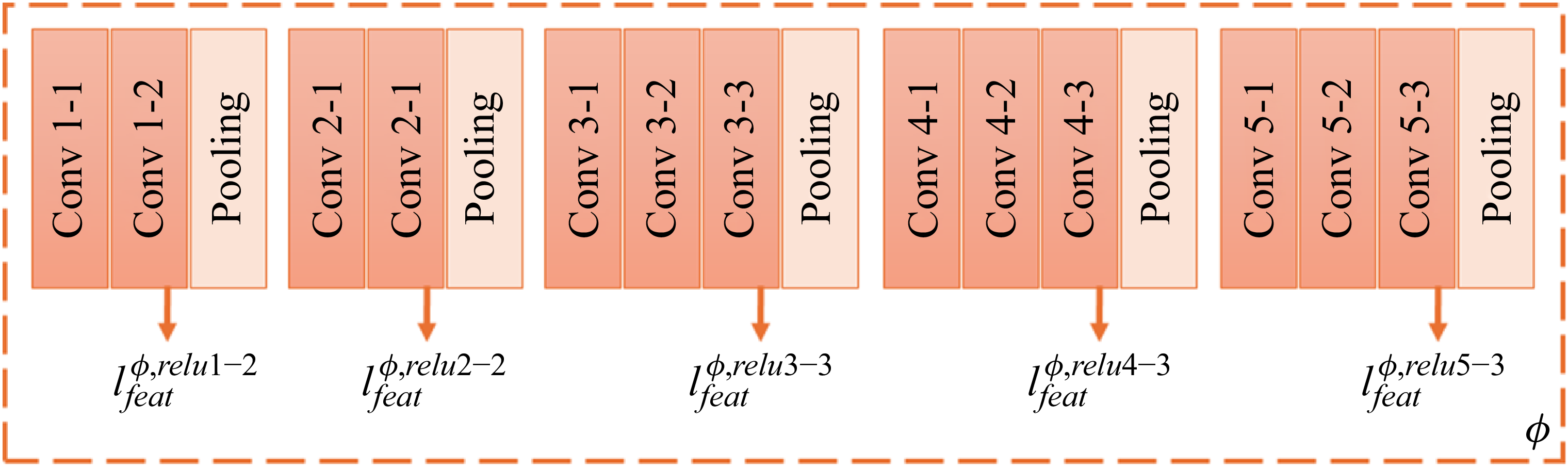


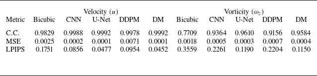


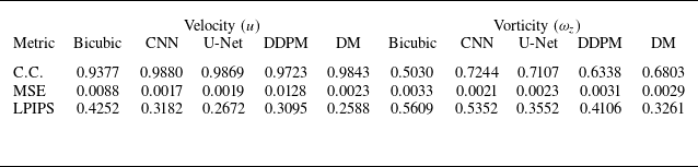


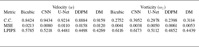


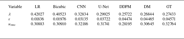
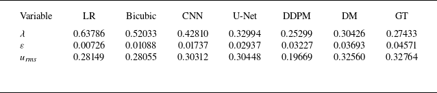
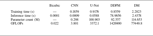


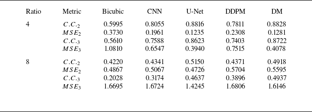


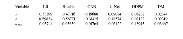


 Open access