


Recent historical trends in binge drinking appear to show distinct developmental variation across the transition to adulthood, covering ages 18–30. When pieced together, historical analyses based on US data collectively suggest this to be true based on cross-sectional data (Cheng et al., Reference Cheng, Cantave and Anthony2016; Grucza et al., Reference Grucza, Norberg and Bierut2009; Keyes & Miech, Reference Keyes and Miech2013; White et al., Reference White, Castle, Chen, Shirley, Roach and Hingson2015) and longitudinal data (Jager et al., Reference Jager, Schulenberg, O’Malley and Bachman2013, Reference Jager, Keyes and Schulenberg2015; Patrick et al., Reference Patrick, Terry-McElrath, Lanza, Jager, Schulenberg and O’Malley2019). Specifically, this work collectively indicates that at the outset of the transition to adulthood (i.e., age 18) binge drinking has decreased across the last three decades. Yet this work also indicates that by the latter half of the transition to adulthood (i.e., mid- to late-20s) binge drinking has increased across the last three decades. This research points to an age by cohort interaction (i.e., cohort differences that vary by age) during the transition to adulthood that is so pronounced that it culminates in historical trends actually reversing across age. In addition to historical trends reversing across age, there is emerging evidence to suggest a “sex convergence” in binge drinking, such that the gap between men and women in binge drinking has narrowed historically (Grucza et al., Reference Grucza, Sher, Kerr, Krauss, Lui, McDowell, Hartz, Virdi and Bierut2018; Keyes et al., Reference Keyes, Jager, Mal-Sarkar, Patrick, Rutherford and Hasin2019; White et al., Reference White, Castle, Chen, Shirley, Roach and Hingson2015).
The public health implications of this reversal (i.e., binge drinking decreasing at age 18 and increasing in the late 20s) are clearly mixed; presumably, recent cohorts face fewer harms associated with binge drinking at the outset of the transition to adulthood, yet face more harms associated with binge drinking during the latter half of the transition to adulthood. Accordingly, any response, whether by policy makers or practitioners, that seeks to maximize the public health benefits and minimize the public health costs of this reversal must be sufficiently nuanced to attenuate the reversal without attenuating age 18 declines. Such a targeted response requires a clearer understanding of the timing of the reversal with respect to both developmental time (i.e., when within the age 18–30 age band the reversal is most pronounced) and historical time (i.e., when over the last three decades the reversal is most pronounced). After all, more accurately localizing when this reversal emerges developmentally within the 18–30 age band will better position policy makers and other stakeholders to target the specific ages when the reversal chiefly manifests. Additionally, more clearly localizing when this reversal emerges historically will clarify whether the historical trends that underlie the reversal are still ongoing among recent cohorts. If the reversal is dissipating among recent cohorts such that age 18 declines are better maintained throughout the 18–30 age band, then perhaps no intervention is necessary. However, if the reversal is still ongoing or even accelerating among recent cohorts, then the size of the reversal may expand moving forward, potentially indicating that that during the latter part of the transition to adulthood future cohorts may face even more harms associated with binge drinking than contemporary cohorts do. Despite its public health implications, our understanding of the reversal is limited. Indeed, no research to date has focused its inquiry on the reversal, and of the available work suggesting a reversal, the reversal was only explicitly mentioned or discussed in one study (i.e., Jager et al., Reference Jager, Keyes and Schulenberg2015).
More fully delineating the timing or when the reversal emerges requires an approach that carefully considers developmental time (i.e., age), historical time (i.e., cohort), as well as their interaction. Such an approach can identify how the age by cohort interaction that underlies the reversal varies developmentally and, in doing so, localize when within the 18–30 age band the age by cohort interaction, and in turn the reversal, is the strongest. Additionally, such an approach can identify whether the magnitude of this age by cohort interaction has varied historically across the last three decades and, in doing so, localize when historically this reversal emerges. However, when it comes to capturing the interplay between developmental and historical time, existing research is limited in several ways. First, the vast majority of research is based on cross-sectional data of successive cohorts, which are limited in disentangling age effects from cohort effects (Karlamangla et al., Reference Karlamangla, Zhou, Reuben, Greendale and Moore2006; Keyes et al., Reference Keyes, Jager, Mal-Sarkar, Patrick, Rutherford and Hasin2019). Second, aside from Patrick et al. (Reference Patrick, Terry-McElrath, Lanza, Jager, Schulenberg and O’Malley2019), existing work only focuses on earlier segments of the 18–30 age band, limiting our knowledge of how the reversal unfolds during the mid- to late 20’s. Third, aside from two important exceptions (i.e., Cheng et al., Reference Cheng, Cantave and Anthony2016; Patrick et al., Reference Patrick, Terry-McElrath, Lanza, Jager, Schulenberg and O’Malley2019), existing work incorporates broad age bins (i.e., collapses age bands together) when assessing how cohort effects vary by age. In doing so, less precise assessments of the interplay between age and cohort are produced, therefore overlooking how cohort effects may vary within these age bands (Cheng et al., Reference Cheng, Cantave and Anthony2016). Fourth, aside from a few exceptions (Jager et al., Reference Jager, Schulenberg, O’Malley and Bachman2013, Reference Jager, Keyes and Schulenberg2015), existing work incorporates broad cohort bins (i.e., collapses cohorts together) when assessing how cohort effects vary by age. In doing so, this existing work also yields less precise assessments of the interplay between age and cohort because it overlooks how age effects may vary within these cohort bands (a detailed comparison of existing work to the work completed as part of this manuscript is provided within The Current Study section). Consequently, while there is mounting evidence to suggest that historical trends in binge drinking during the transition to adulthood reverse across age due to an age by cohort interaction, whether this reversal gradually emerges across developmental time (or instead is primarily localized to specific ages) and historical time (or instead is primarily localized to specific cohorts) remains unclear, which in turn make for imprecise policy implications.
Further, we know even less about why (i.e., underlying mechanisms) this reversal emerges. Existing work is largely drawn from cross-sectional surveillance sources that are ill equipped to answer mechanistic questions compared to historical–longitudinal data. Importantly, delineating why historical trends reversed across age would provide important leverage for intervention and policy aimed at reducing binge drinking and its corresponding risks among current and future cohorts of transitioning adults. To address these gaps, we use multi-cohort longitudinal data from the US national multi-cohort Monitoring the Future panel study (MTF; (Schulenberg et al., Reference Schulenberg, Johnston, O’Malley, Bachman, Miech and Patrick2020) to provide a more precise accounting of when and why historical trends in binge drinking frequency and prevalence reversed across age. To do so, we build on our previous work utilizing MTF data focused on both binge drinking frequency (Jager et al., Reference Jager, Schulenberg, O’Malley and Bachman2013, Reference Jager, Keyes and Schulenberg2015) and prevalence (Patrick et al., Reference Patrick, Terry-McElrath, Lanza, Jager, Schulenberg and O’Malley2019) during the transition to adulthood. Although our previous work used appropriate analytic strategies for the given research questions, here, in order to better capture the reversal in binge drinking, we extend this work by applying different analytical techniques (see The Current Study section for a detailed description) that allow us to more accurately localize when – both developmentally and historically – and why the age by cohort interaction that underlies the reversal emerges. Additionally, we also pay particular attention to whether age, cohort, and their interaction vary by sex. After all, regarding a potential sex convergence, intervention and prevention efforts require more specific information regarding when – both developmentally and historically – and why this sex convergence occurred.
Directing attention to why historical trends in binge drinking reversed across age
Both the ecological model of human development (Bronfenbrenner, Reference Bronfenbrenner1994) and the developmental–contextual model of addictions (e.g., (Schulenberg et al., Reference Schulenberg, Maslowsky, Jager, Fitzgerald and Puttler2018; Zucker & Gomberg, Reference Zucker and Gomberg1986) provide a useful theoretical framework for capturing why (i.e. underlying mechanisms) historical trends in binge drinking have reversed across age. In the ecological model of human development (Bronfenbrenner, Reference Bronfenbrenner1994), the chronosystem is the most distal context within one’s ecology and encompasses socio-historical variation in society-level factors, such as opportunity structures, life-course options, and public policies. The developmental–contextual model of addictions (e.g., Schulenberg et al., Reference Schulenberg, Maslowsky, Jager, Fitzgerald and Puttler2018; Zucker & Gomberg, Reference Zucker and Gomberg1986), which is consistent with other multi-level developmental conceptual models in developmental science (e.g., Lerner, Reference Lerner2007; Sameroff, Reference Sameroff2010) and developmental psychopathology (e.g., Belsky, Reference Belsky1981, Reference Belsky1993; Cicchetti et al., Reference Cicchetti, Toth, Maughan, Sameroff, Lewis and Miller2000; Cicchetti & Rogosch, Reference Cicchetti and Rogosch2002; Schulenberg et al., Reference Schulenberg, Sameroff and Cicchetti2004) views substance use as the product of transactions among forces within the individual and ecological contexts. Though individuals play an active role in their own development, they are also influenced by the immediate contexts surrounding them, and those contexts are, in turn, influenced by more distal society-level factors. Thus, historical variation in young adult binge drinking likely entails layered interactions between bottom-up and top-down factors that when taken as a whole, help explain ongoing chronosystem effects.
Regarding why (i.e., underlying mechanisms) historical variation in binge drinking has manifested, research has focused on Big5 social roles (marriage, employment, college attendance, parenthood, and residential independence; Settersten et al., Reference Settersten, Ottusch and Schneider2015) and minimum legal drinking age (MLDA) because both are strong determinants of alcohol use and both have varied historically. Due largely to historical variation in labor force structures and employment options (i.e., chronosystem effects), today’s young adults are more likely to hold social roles associated with more binge drinking (i.e., going to college full-time) and are more likely to delay transition to social roles associated with less binge drinking (i.e., working full-time, getting married, having children, residential independence) (Jager et al., Reference Jager, Keyes and Schulenberg2015; White et al., Reference White, Labouvie and Papadaratsakis2005). Regarding MLDA, due to changes in federal policy (i.e., chronosystem effects), between 1985 and 1987 thirty-one states increased their MLDA from either 18, 19, or 20 to age 21 (Hedlund et al., Reference Hedlund, Ulmer and Preusser2001; Wagenaar & Toomey, Reference Wagenaar and Toomey2002). Following these changes, alcohol consumption decreased among the cohorts that used to be of legal drinking age prior to the law change (Wagenaar & Toomey, Reference Wagenaar and Toomey2002).
While a wealth of research has examined how social roles and MLDA are associated with binge drinking, to our knowledge only Jager et al (Reference Jager, Keyes and Schulenberg2015) and Patrick et al. (Reference Patrick, Terry-McElrath, Lanza, Jager, Schulenberg and O’Malley2019) have more specifically examined whether historical variation in social roles and MLDA are associated with historical variation in binge drinking. Both Jager et al. (Reference Jager, Keyes and Schulenberg2015) and Patrick et al. (Reference Patrick, Terry-McElrath, Lanza, Jager, Schulenberg and O’Malley2019) found that cohort differences in age trends (i.e., age by cohort interactions) of binge drinking were attenuated, but still significant, after controlling for cohort differences in social roles and MLDA. Jager et al., (Reference Jager, Keyes and Schulenberg2015) went on to test and find that the attenuating effects of social roles and MLDA were both significant, indicating partial mediation, and historically broad (i.e., attenuating effects were stable across the cohorts examined). However, because Jager et al. (Reference Jager, Keyes and Schulenberg2015) only examined the combined attenuating effects of social roles, the specific attenuating effects of marriage, college status, employment status, parenthood and residential independence remain unclear. Additionally, because Jager et al. (Reference Jager, Keyes and Schulenberg2015) relied on broad age bins, it remains unclear whether the attenuating effects of social roles and MLDA are primarily localized to specific ages. Thus, whereas existing work does indicate that historical variation in social roles and MLDA does partially mediate historical variation in binge drinking, it does not more specifically indicate whether the developmental timing of that mediation is in-sync with when historical variation in binge drinking is most pronounced. Identifying whether the ages at which effects of the mediators are most pronounced is in-sync with the ages at which historical variation in binge drinking is most pronounced is important, because to the extent that they are not in-sync, the mediators are less effective intervention targets.
Sex differences in the effects of chronosystem factors may explain why a sex convergence has occurred. As mentioned above, today’s young adults are more likely to hold social roles associated with more binge drinking. Ample evidence suggests that this trend has been more pronounced for women (Mortimer, Reference Mortimer2015), potentially resulting in a narrowing of sex differences. Additionally, although Jager et al. (Reference Jager, Keyes and Schulenberg2015) did not formally compare effects across sex, they did find evidence to suggest that the dampening effect of raising MLDA on binge drinking was larger for men. Thus, potentially increasing MLDA led to greater decreases in binge drinking among men than women, also resulting in a narrowing of sex differences.
The current study
Historical analyses based on US data indicate that although recent cohorts engage in lower binge drinking at age 18 relative to past cohorts, by the latter half of the transition to adulthood the reverse is true: recent cohorts engage in higher binge drinking during the mid- to late-20s relative to past cohorts. Using US national, longitudinal data from the Monitoring the Future project (MTF; Schulenberg et al., Reference Schulenberg, Johnston, O’Malley, Bachman, Miech and Patrick2020) that span over three decades of historical time (i.e., 31 consecutive cohorts of graduating high-school seniors from 1976 to 2006) and span the entirety of the transition to adulthood (i.e., ages 18–30), we direct our attention to not just when but also to why historical trends in binge drinking frequency reversed across age. Our study, which is the first to focus directly on this reversal, expands upon existing work, including our own (Jager et al., Reference Jager, Schulenberg, O’Malley and Bachman2013, Reference Jager, Keyes and Schulenberg2015; Patrick et al., Reference Patrick, Terry-McElrath, Lanza, Jager, Schulenberg and O’Malley2019), in four important ways. First, whereas the majority of the existing research that examines historical variation in developmental trends in binge drinking has focused on prevalence, here we focus on both binge drinking frequency and prevalence. We do so because the degree and pattern of developmental and historical trends in binge drinking frequency do not necessarily parallel those of binge drinking prevalence (Dawson et al., Reference Dawson, Goldstein, Saha and Grant2015; Karlamangla et al., Reference Karlamangla, Zhou, Reuben, Greendale and Moore2006; Moore et al., Reference Moore, Gould, Reuben, Greendale, Carter, Zhou and Karlamangla2005; White et al., Reference White, Castle, Chen, Shirley, Roach and Hingson2015). Second, to assess developmental variation in the age by cohort interaction that underlies the reversal with maximal specificity, we specify cohort as an age-varying predictor within latent growth models of age 18–30 binge drinking. Additionally, to assess cohort with maximal specificity, we treat cohort continuously (as opposed to categorically based on broader cohort bins) to identify whether these age-specific trends in the age by cohort interaction emerge more steadily and gradually (i.e., linearly) or more sporadically (i.e., curvilinearly) across historical time. In doing so, we yield a more precise accounting of when developmentally (within the 18–30 age band) and when historically (within the 31 cohorts examined here) the age by cohort interaction that underlies the reversal manifested and why it manifested. Third, with respect to why the reversal manifested, unlike previous work, which identified the aggregate contributions of social roles and MLDA, we identify both the aggregate and specific contributions, and more precisely specify the developmental timing of those contributions. Fourth, we also formally test for sex differences in when and why historical trends in binge drinking frequency reversed across age. There are two overarching aims: (1) to delineate when developmentally and historically the across-age reversal in binge drinking frequency manifested and test for sex differences; and (2) to examine why the reversal manifested by testing the unique and combined contributions of historical variation in social roles and MLDA and test for sex differences.
Method
Respondents and procedure
MTF is an ongoing US national study of the epidemiology and etiology of drug use among adolescents and adults (Miech et al., Reference Miech, Johnston, O’Malley, Bachman, Schulenberg and Patrick2020; Schulenberg et al., Reference Schulenberg, Johnston, O’Malley, Bachman, Miech and Patrick2020). Beginning in 1975, U.S. samples of approximately 16,000 12th graders were drawn from about 135 public and private schools each year (Miech et al., Reference Miech, Johnston, O’Malley, Bachman, Schulenberg and Patrick2020). Beginning with the class of 1976, approximately 2,400 respondents were randomly selected for biennial follow-up from each cohort through mail surveys, with one random half being surveyed 1 year after high school and the other random half being surveyed 2 years after high school; each half was followed biennially thereafter (Schulenberg et al., Reference Schulenberg, Johnston, O’Malley, Bachman, Miech and Patrick2020). Respondents who reported illicit drug use at baseline were oversampled for follow-up; corrective weighting was used in the analyses. The full sample was predominantly White (75.4%), evenly split by sex (50.9% female), and, on average, had parents who completed some college. This study was approved by the IRB at University of Michigan.
In the present study we focused on data for ages 18 to 30, which correspond to the first 7 waves of the MTF panel data. Respondents were, on average, 18 years old at Wave 1, 19–20 years old at Wave 2, 21–22 years old at Wave 3, 23–24 years old at Wave 4, 25–26 years old at Wave 5, 27–28 at Wave 6, and 29–30 at Wave 7. For the purposes of this study, analyses were limited to those respondents who were in 12th grade between 1976 and 2006, and who provided data at one or more waves (N = 75,744). Data extend until 2018, when the 2006 cohort was aged 29–30. Wave to wave retention rates between Waves 1 and 7 were 72.25%, 94.06%, 94.13%, 93.45%, 94.76%, and 93.87%, respectively. The retention rate between Waves 1 and 7 was 53.18% on average across cohort. Across the 31 (i.e., 1976–2006) cohorts examined here, sample sizes at age 18 ranged from 2,497 to 2,224, and sample sizes at age 30 ranged range from 1,628 to 1,045 per cohort. These retention rates reflect the reality of long-term longitudinal studies of drug use (Hansen et al., Reference Hansen, Tobler and Graham1990; McCabe & West, Reference McCabe and West2016) and compare reasonably well with other long-term studies (Booker et al., Reference Booker, Harding and Benzeval2011). Attrition analyses indicated that compared to those lost, those retained through Wave 7 were more likely to be female, to be white, to live in non-urban areas, to report a higher high school GPA, to have more educated parents who are married, and to report lower senior year substance use, including binge drinking. These analyses also indicated that attrition rates were higher among recent cohorts, consistent with what is occurring with other longitudinal studies (Galea & Tracy, Reference Galea and Tracy2007). Though statistically significant, the effects of attrition were small in magnitude (i.e., R 2 = .03 for high school GPA and race/ethnicity, R 2 = .02 for sex, and R 2 < .005 for all other variables, including binge drinking). Additionally, those who attrited (in terms of race/ethnicity, sex, H.S. GPA, alcohol consumption, and binge drinking) did not meaningfully vary by cohort (i.e., all R 2 < .003). Thus, effects of attrition, including differential attrition across cohort, on sample estimates are minimal. Consistent with recent MTF analyses (McCabe et al., Reference McCabe, Veliz, Boyd and Schulenberg2017, Reference McCabe, Veliz, Boyd, Schepis, McCabe and Schulenberg2019; Schulenberg et al., Reference Schulenberg, Patrick, Kloska, Maslowsky, Maggs and O’malley2015), we incorporated combination attrition/sample weights that account for both the oversampling of persons who engage in drug use into the panel as well as respondent characteristics associated with nonresponse at age 29–30 follow-up to correct for potential attrition bias.
Measures
Binge drinking
Each survey, respondents were asked to think back over the last 2 weeks when answering the question, “How many times have you had five or more drinks in a row?” with response options of none, once, twice, 3–5 times, 6–9 times, and 10 or more times. For frequency, binge drinking was coded to approximate a continuous measure of frequency: “none” = 0; “once” = 1; “twice” = 2; “3–5 times” = 4, “6–9 times” = 7.5, and “10 or more times” = 10. For prevalence, binge drinking was coded as a dichotomous variable indicating any consumption of five or more drinks in a row during the last 2 weeks (yes, no).
Cohort
The measure cohort ranged from 0 to 30 and was based on the year that respondents were seniors in high school (i.e., 1976 seniors = 0, 1977 seniors =1, and so forth). To assess linear trends in cohort we mean-centered the measure of cohort and then divided it by 10 to re-scale it to decades (range from −1.5 to 1.5, with the 1991 cohort equal to 0). We then squared this measure to assess quadratic trends in cohort. Preliminary analyses indicted that the inclusion of higher-order cohort polynomials, such as cubic, were not warranted (see results section for more details).
Social roles
At each wave we dichotomized indicators of respondent marital status, full-time employment status (e.g., working 35 or more hr/week), full-time college status, parental status, and residential independence (i.e., not living with parents). All indicators were self-report, and all indicators were available at each wave, with the exception of full-time college status and full-time employment, which were not available at Wave 1 because all participants at that age were surveyed in high school. A more detailed summary of the social role measures can be found in Jager et al (Reference Jager, Keyes and Schulenberg2015).
Minimum legal drinking age (MLDA)
MLDA was based on self-reported state residency as well as data on state-level changes in MLDA compiled by others (Hedlund et al., Reference Hedlund, Ulmer and Preusser2001; Wagenaar & Toomey, Reference Wagenaar and Toomey2002). Based on these data, we determined each respondent’s state’s MLDA at each wave, with a possible range of 18 to 21. Where possible, we allowed for changes in state residency across waves. However, prior to 1987 state residency was asked at Wave 1 only. Therefore, for data collected prior to 1987, state residency at Waves 2–7 was based on state residency at Wave 1. At Wave 7 MLDA is nearly uniformly age 21 (because all of the data provided falls after 1998 and thus largely after the period MLDA was increased across the U.S.). Due to insufficient variance, MLDA at Wave 7 is not included in the analyses.
Analytical plan
Analyses were conducted with Mplus Version 8 (Muthén & Muthén, Reference Muthén and Muthén2017). We used Kline’s (Reference Kline2015) guidelines to assess model fit: RMSEA smaller than .05 represents close fit and CFI larger than .95 indicates excellent fit. Preliminary analyses indicated that sex differences and historical trends in binge drinking did not vary based on whether individuals were randomly followed-up 1-year versus 2-years after baseline. Thus, to eliminate unnecessary complexity here the two random halves of each cohort are combined in all analyses. Hereafter, for simplicity we only refer to the even-numbered ages when referring to the ages that correspond to waves.
Because substance use typically shows a positively skewed distribution, for analyses of binge drinking frequency we used an identity link in conjunction with a robust maximum likelihood sandwich estimator that is robust to non-normality. For analyses of binge prevalence, we also used an identity link (as opposed to a non-linear logit link) in conjunction with a robust maximum likelihood sandwich estimator that is robust to non-normality. We did so because when comparing effects across age and across sex we are interested in absolute differences in binge drinking prevalence – or risk differences – which are obtained via an identity link function, as opposed to relative differences in binge drinking prevalence – or odds ratios and risk ratios – which are obtained via a non-linear logit link function (Cheung, Reference Cheung2007; Schechtman, Reference Schechtman2002; Sinclair & Bracken, Reference Sinclair and Bracken1994). Simulation studies have shown (Cheung, Reference Cheung2007), including those utilizing nested data (Pedroza & Thanh Truong, Reference Pedroza and Thanh Truong2016; Ukoumunne et al., Reference Ukoumunne, Forbes, Carlin and Gulliford2008), that an identity link function used in conjunction with a robust maximum likelihood sandwich estimator reliably produces unbiased estimates and standard errors of risk difference in binary outcomes. As a robustness check we replicated all analyses of binge drinking frequency and prevalence – including analyses estimating indirect effects as described below for Aim 2 – using bias-corrected non-parametric bootstrapping (MacKinnon et al., Reference MacKinnon, Lockwood and Williams2004). Here we took a conservative approach and set the number of bootstraps to be 3,000 as opposed to the standard number of 1,000 bootstraps (MacKinnon et al., Reference MacKinnon, Lockwood and Williams2004; Tofighi & MacKinnon, Reference Tofighi and MacKinnon2016). Given our use of a robust maximum likelihood estimator, all model comparisons were tested via the appropriate adjustment equations (Satorra & Bentler, Reference Satorra and Bentler2001). Given this study’s large sample size, for all analyses we utilized a conservative .01 α level.
Aim 1. Delineating when the reversal manifested
We used a piece-wise latent growth model (Li et al., Reference Li, Duncan, Duncan and Hops2001) to assess age 18 to 30 trajectories (i.e., age main effects) of binge drinking. Using the model in Figure 1, we estimated the following factors: (1) age 18 intercept; (2) age 18–22 linear growth; (3) age 22–26 linear growth; and (4) age 26–30 linear growth. As a sensitivity analysis, we specified a more conventional latent growth model with linear, quadratic, and cubic growth factors. Although models utilizing this alternative specification provided equivalent results to the models using the piece-wise specification, they proved to be less stable.
Piece-wise latent linear growth model with cohort polynomials as age-varying predictors.

We capture age-varying effects of cohort by specifying the linear and quadratic cohort polynomials as predictors of each binge drinking indicator (See gray portion within Figure 1). At each age, these effects capture whether cohort is associated with deviations from predicted values of binge drinking based on the overall growth trajectory. Cohort main effects are captured by the across-age average of the effects of cohort polynomials, whereas cohort by age interactions are captured by across-age variation in the effects of the cohort polynomials. Cohort main effects (i.e., across-age averages) were determined by models constraining cohort effects to be the same across age. Cohort by age interactions (i.e., across age variation in the effects of the cohort polynomials) were determined via chi-square difference tests (e.g., model fit where effects are constrained to be the same across age is compared to model fit where effects are free to vary across age). A reversal will be indicated by cohort effects that not only increase across age but more specifically go from negative at age 18 (indicating declines across cohort at age 18) to positive at age 30 (indicating increases across cohort at age 30).
Aim 2. Contribution of potential mediators (chronosystem factors) to the reversal
Building on the model in Figure 1, we estimated the direct effects of cohort as well as the indirect effects of cohort (i.e., through the social role and MLDA mediators) on each binge drinking indicator. We did so to determine the amount of across-age averaged effects of cohort (cohort main effects) and age-varying effects of cohort (cohort by age interactions) that is directly explained by cohort versus indirectly explained by the mediators (i.e., accounted for by indirect effects). To aid in interpretation of growth factors, each social role was mean-centered at each wave so that intercepts of the binge drinking indicators reflect overall sample averages. Additionally, MLDA was centered around age 21 at each wave so that intercepts of the binge drinking indicators reflect predicted values under the condition that MLDA was uniformly age 21 across all cohorts. Building on the model in Figure 1, we specified at each wave: (i) paths from each cohort polynomial to each available social role and MLDA (i.e., “a” paths from predictor to mediators); and (ii) paths from each available social role and MLDA to that wave’s binge drinking indicator (i.e., “b” paths from mediators to outcome; see Supplemental Figure 1). We used the model constraint command to calculate indirect effects by specifying the product of corresponding “a” and “b” paths and then calculate for each wave the combined indirect effects for all available social roles and MLDA as well as specific indirect effects for all available social roles and MLDA. Direct effects of the cohort polynomials were estimated by the direct paths from each cohort year polynomial to each binge drinking indicator (See Supplemental Figure 1).
Estimating sex differences
To model sex differences within both the Aim 1 and Aim 2 analyses, we conducted multiple group analyses with sex as a grouping variable. To estimate sex differences we used the model constraint command in Mplus (Muthén & Muthén, Reference Muthén and Muthén2017) to create new model parameters that subtracted corresponding estimates of women from men. The estimates for these new model parameters as well as their standard errors were calculated within Mplus. Negative values are indicative of sex convergence or a decrease in sex differences whereas positive values are indicative of sex divergence or an increase in sex differences. Example Mplus syntax for Aims 1 and 2 are provided in Appendices A and B, respectively.
Results
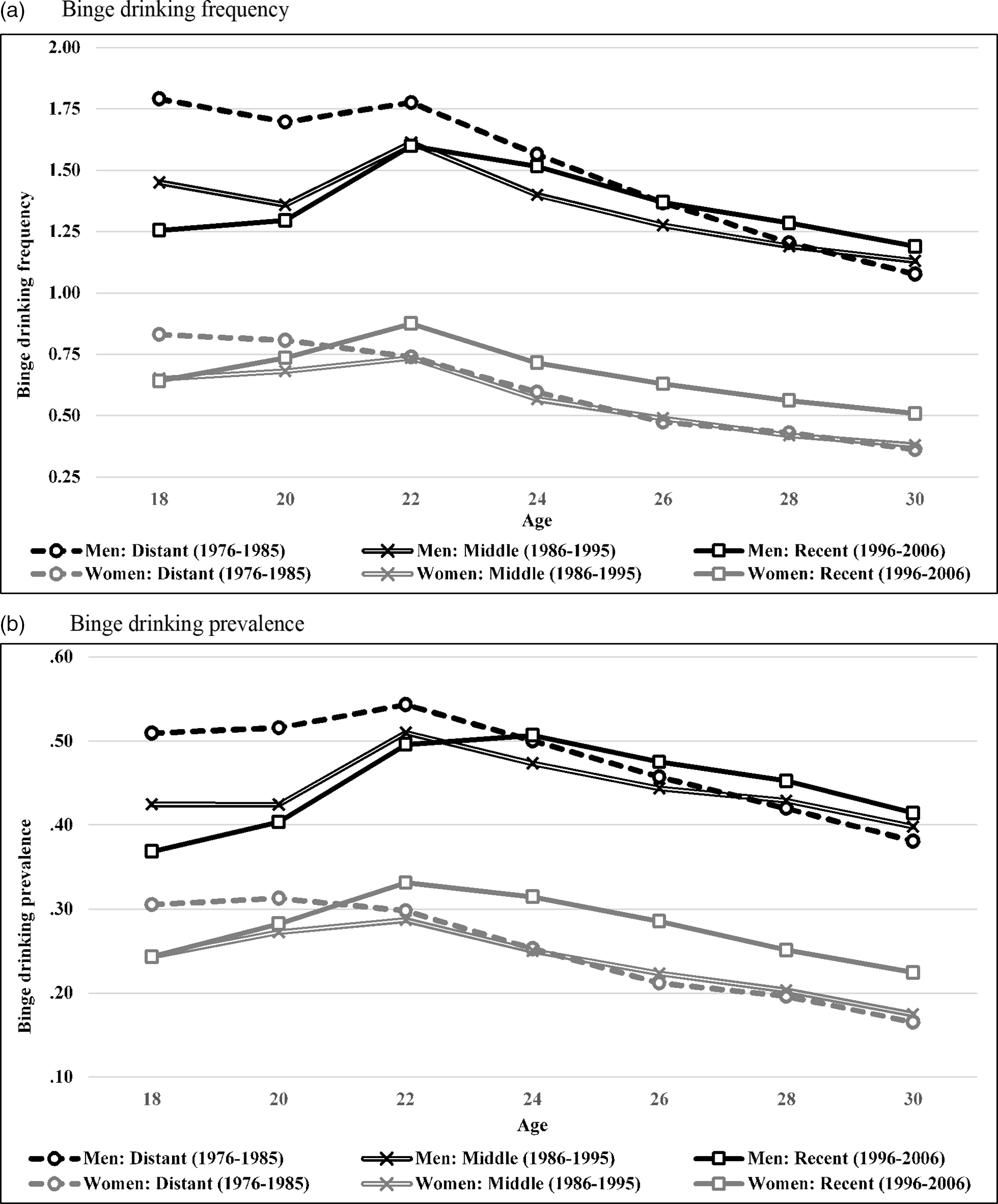
The fit of each model tested was excellent; thus, given space constraints, fit indices for each model are not discussed but are provided within table notes. Means, SDs, and prevalence rates for binge drinking, as well as means for each of the social roles and MLDA are presented in Table 1 separately by age and sex. To provide a descriptive summary of historical variation in age 18–30 trajectories of binge drinking frequency and prevalence (Figure 2), we created three cohort groups by dividing the 31 cohorts examined here into roughly equal thirds: (1) “Distant” (1976–1985 cohorts); (2) “Middle” (1986–1995 cohorts); and (3) “Recent” (1996–2006 cohorts). The across-age reversal in historical trends in binge drinking is clearly illustrated in Figure 2 for both frequency and risk: for both men and women, recent cohorts display both the lowest binge drinking at age 18 and the highest binge drinking at age 30. When applying our .01 alpha level for model comparisons, the inclusion of quadratic cohort polynomials (over and above linear cohort polynomials) resulted in significant improvement in model fit for both binge frequency, χ 2 (14) = 72.46, p < .001, and prevalence, χ 2 (14) = 98.58, p < .001. However, the addition of cubic cohort polynomial predictors (over and above linear and quadratic cohort polynomials) did not result in a significant improvement in model fit for both binge frequency, χ 2 (14) = 25.94, p = .026, and prevalence, χ 2 (14) = 22.52, p = .068. Consequently, when testing for age-varying effects of cohort, only linear and quadratic polynomial predictors are included.
Descriptives for binge drinking and chronosystem factors by sex and age

Notes. FT = full-time. Res. Ind. = residential independence. MLDA = minimum legal drinking age. NA = not available due to lack of measurement. All descriptives listed are across-cohort averages.
Age 18–30 trajectories of binge drinking by sex and historical cohort group. Trajectories are based on weighted means (using combination sample/attrition weights). For frequency the Y-axis represents number of occasions, last 14 days; for prevalence the Y-axis represents prevalence rates, last 14 days.
Preliminary analyses: age and cohort main effects
Age main effects (all cohorts combined)
Age main effects are indicated by the estimates of growth factors presented in Table 2. Across ages 18–30, binge drinking frequency and prevalence followed an inverted-U shaped pattern characterized by increases across ages 18–22 and decreases across ages 22 to 30. This inverted-U shaped pattern is consistent with binge drinking means in Table 1 as well as the extensive work documenting normative age trends in binge drinking across the transition to adulthood (Chen et al., Reference Chen, Dufour and Yi2005; Lee & Sher, Reference Lee and Sher2018; Schulenberg et al., Reference Schulenberg, Johnston, O’Malley, Bachman, Miech and Patrick2020). We also found evidence for sex by age interactions for both binge drinking frequency and prevalence. At age 18, men displayed greater binge drinking for both frequency (.797) and prevalence (.169). The pace of increases across ages 18–22 was faster for men for both frequency (.061) and prevalence (.025), indicating sex divergence or an expansion of sex differences. For frequency only the pace of decreases across ages 22–26 (−.033) and 26–30 (−.038) was slower for women, indicating sex convergence or a contraction of sex differences.
Age 18 to 30 growth in binge drinking frequency and prevalence and age-varying cohort effects by sex
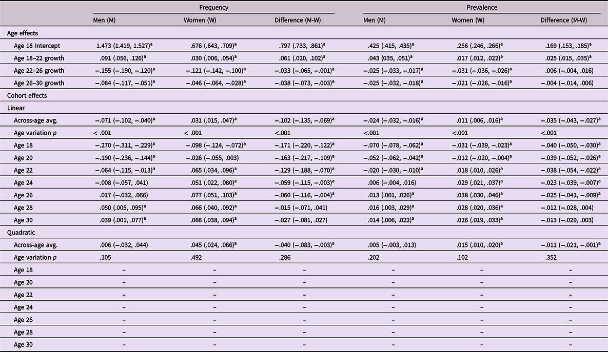
Notes. All estimates are unstandardized. 99% confidence intervals are listed in parentheses. Cohort is scaled to decades (i.e., an increase of 1.0 equals 1 decade or 10 years).
a Statistically significant findings (99% confidence interval excludes 0). Age variation p values are based on chi-square difference tests; age-varying effects are not provided and instead are displayed as “–” when the age variation p is ≥ .01. Model fit for frequency: χ 2(28) = 111.492, p < .001; CFI = .997; RMSEA = .009. Model fit for risk: χ 2(28) = 76.011, p < .001; CFI = .999; RMSEA = .007.
Cohort main effects (all ages combined)
Cohort main effects are indicated by the across-age average effects of the cohort year polynomials presented in Table 2. Regarding linear effects of cohort, both binge drinking frequency (−.071) and prevalence (−.024) decreased across cohort for men, indicating that, when aggregating across ages 18–30, each decade increase in cohort was associated with a .071 decrease in frequency and a .024 decrease in prevalence from predicted values based on the across-cohort growth trajectory in binge drinking frequency. However, for women each decade increase in cohort was associated with increases from predicted values based on the across-cohort growth trajectory for both frequency (.031) and prevalence (.011). Hereafter we refer to decreases and increases from predicted values based on across-cohort trajectories as “decreases” and “increases” for simplicity. We also found evidence for sex by cohort interactions for both frequency and prevalence. Because frequency and prevalence decreased across cohort for men but increased across cohort for women, when aggregating across ages 18–30, both frequency and prevalence converged across sex such that each decade increase in cohort was associated with a .102 contraction in the sex difference for frequency and a .035 contraction in the sex difference for prevalence.
Quadratic effects of cohort proved non-significant for both binge drinking frequency (.006) and prevalence (.005) for men. However, for women quadratic trends of cohort were positive for both frequency (.045) and prevalence (.015), indicating the pace of cohort increases in both frequency and prevalence, due to linear trends described above, quickened as cohort increased. Sex differences in the quadratic effects of cohort indicate that, when aggregating across ages 18–30, sex convergence for both frequency and prevalence was more pronounced among cohorts that are more recent.
Aim 1: Delineating when the reversal manifested
Cohort by age interactions are indicated by across-age variation in the effects of the cohort year polynomials (see age variation p-values presented in Table 2). For both sexes and for both binge drinking frequency and prevalence, quadratic cohort effects did not vary by age. Additionally, for both binge drinking frequency and prevalence, gender differences in quadratic cohort effects did not vary by age. Consequently, when discussing cohort by age interactions below, we only address those involving linear cohort effects. For an age-specific description of quadratic cohort effects, see Appendix C.
Age by cohort interactions
For binge drinking frequency, linear cohort effects increased across age and ultimately reversed direction for both men (from −.270 at age 18 to .039 at age 30) and women (−.098 at age 18 to .066 at age 30), indicating that age 18 frequency decreased across cohort whereas age 30 frequency increased cohort for both sexes. Findings for prevalence mirrored those for frequency: Linear cohort effects increased across age and ultimately reversed direction for both men (from −.070 at age 18 to .014 at age 30) and women (−.031 at age 18 to .026 at age 30).
Pinpointing when developmentally the reversal manifested
For men the reversal was primarily localized to ages 18–24 for both binge drinking frequency and prevalence because, based on 99% CIs listed in Table 2, linear cohort effects did not differ from one another across ages 24 to 30. Put another way, after age 24, the effect of cohort did not vary across age, which is consistent with Figure 2 (i.e., for men the three cohort group trajectories are relatively parallel with one another across ages 24–30 when compared to ages 18–24). Based once again on 99% CIs of linear cohort effects listed in Table 2, for women the reversal was primarily localized to ages 18–22 for frequency and prevalence, which again is consistent with Figure 2.
Pinpointing when historically the reversal manifested
For both sexes and for both binge drinking frequency and prevalence, we found across age variation (i.e., cohort by age interactions) in linear cohort effects but not quadratic cohort effects. Collectively, these findings indicate that the cohort by age interactions that underlies the reversal are characterized as linear trends and thus emerged gradually and consistently across cohort.
Sex differences in the reversal
Although linear cohort effects for both binge drinking frequency and prevalence increased across age (went from negative at age 18 to positive at age 30) for both men and women, the magnitude of the across-age increase was larger for men (i.e., a sex by cohort by age interaction; Table 2). As a result, for binge drinking frequency the magnitude of sex convergence across cohort dissipated across age. Specifically, at age 18, each decade increase in cohort was associated with a .171 contraction in the sex difference, because men (−.270) decreased faster across cohort than women (−.098). However, at age 30 each decade increase in cohort was associated with a .027 (and non-significant) contraction in the sex difference, because men (.039) and women (.066) increased at the same pace across cohort. For prevalence, the magnitude of the contraction in the sex difference across cohort also dissipated across age: from a .040 contraction at age 18 (due to men decreasing faster across cohort) to a .013 (and non-significant) contraction at age 30 (due to men and women increasing at the same pace across cohort). Collectively, these findings indicate that sex convergence (i.e., narrowing of sex differences across cohort) for frequency and prevalence was largest at age 18 and then contracted through age 30 such that the contraction at age 30 proved non-significant.
Aim 2. Contribution of potential chronosystem mediators to the reversal
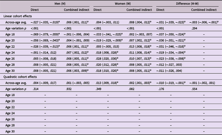
For binge drinking frequency and prevalence, respectively, Tables 3 and 4 list for each sex the portion of the total cohort effect for each age that is independent of social roles and MLDA (see direct effects) as well as the portion of the total cohort effect for each age that is collectively mediated through social roles and MLDA (see combined indirect effects). Corresponding estimates for direct and indirect effects of sex differences are also listed within Tables 3 and 4. Estimates for the specific indirect effects of each social role and MLDA are provided in Supplemental Tables 1 through 6. Estimates for the “a” and “b” baths used to derive indirect effects are provided in Supplemental Tables 7 and 8, respectively. Direct and indirect quadratic cohort effects are only discussed in the rare instances that they varied by age. For a fuller discussion of direct and indirect quadratic cohort effects, see Appendix B.
Direct and combined indirect effects of cohort on binge drinking frequency by sex

Notes. All estimates are unstandardized. 99% CI are listed in parentheses. Cohort is scaled to decades (i.e., an increase of 1.0 equals 1 decade or 10 years).
a Statistically significant findings (99% CI excludes 0). Age variation p values are based on chi-square difference tests; age-varying effects are not provided and instead are displayed as “–” when the age variation p is ≥ .01. Model fit: χ 2(496) = 2608.109, p < .001; CFI = .997; RMSEA = .011.
Direct and combined indirect effects of cohort on binge drinking prevalence by sex
Notes. All estimates are unstandardized. 99% CI are listed in parentheses. Cohort is scaled to decades (i.e., an increase of 1.0 equals 1 decade or 10 years).
a Statistically significant findings (99% CI excludes 0). Age variation p values are based on chi-square difference tests; age-varying effects are not provided and instead are displayed as “–” when the age variation p is ≥ .01. Model fit: χ 2(496) = 2718.191, p < .001; CFI = .996; RMSEA = .011.
Findings generally indicate that for both sexes and for both binge drinking frequency and prevalence, social roles and MLDA accounted only to a small extent for the across-age reversal in cohort effects. For frequency, direct linear cohort effects increased across age and ultimately reversed direction for both men (from −.262 at age 18 to .016 at age 30) and women (−.112 at age 18 to .047 at age 30). The scope of these age declines in linear cohort effects were only slightly reduced from the overall or “total” linear cohort effects listed in Table 2 for men (from −.270 at age 18 to .039 at age 30) and women (from −.098 at age 18 to .066 at age 30). Findings for prevalence mirrored those for frequency.
Although small in comparison to direct effects, combined linear effects were generally positive, indicating that historical variation in social roles and MLDA contributed to historical increases in binge drinking frequency and prevalence. Combined linear effects were generally evident across the entire 18–30 age band; however, they did vary by age and were largest either in the middle portion (frequency for both sexes and prevalence for women) or latter portion of the 18–30 age band (prevalence for men). The finding that combined linear effects were more positive at older ages suggests that historical declines at age 18 would have been better maintained through age 30 in the absence of historical variation in social roles and MLDA. For both sexes and for both frequency (see Supplemental Tables 1–2) and prevalence (see Supplemental Tables 3–4), combined indirect linear effects were primarily a function of the following specific indirect linear effects that all varied by age: (1) marriage (largest in the middle portion of the 18–30 age band); (2) full-time college (only evident in the initial portion of the 18–30 age band); (3) parenthood (generally increased with age); and (4) residential independence (reversed direction from negative to positive across age).
Sex differences
Findings clearly indicate that age declines in the magnitude of sex convergence (i.e., sex convergence across cohort being more pronounced at age 18 than age 30) were largely unexplained of social roles and MLDA. In terms of direct linear cohort effects, the magnitude of sex convergence across cohort declined across age for binge drinking frequency (from −.149 at age 18 to −.031 at age 30; Table 3) and prevalence (from −.037 at age 18 to −.011 at age 30; Table 4). The scope of these age declines in sex convergence were only slightly reduced from the overall or “total” sex differences in linear cohort effects listed in Table 2 for frequency (from −.171 at age 18 to −.027 at age 30) and prevalence (from .040 at age 18 to −.013 at age 30).
Although small in comparison to direct effects, for binge drinking frequency and prevalence (See Supplemental Tables 5 and 6), sex differences in combined indirect linear effects were primarily a function of sex differences in indirect linear effects specific to marriage, which varied by age. For frequency, marriage contributed to sex convergence during the early portion of the age 18–30 age band (because although specific indirect effects were positive for both sexes, they were more positive for women), but contributed to sex divergence during the latter portion of the age 18–30 age band (because although specific indirect effects were positive for both sexes, they were more positive for men). For prevalence, marriage contributed to sex convergence (because although specific indirect effects were positive for both sexes, they were more positive for women), but this effect reduced to non-significance by the end of the 18–30 age band. For binge frequency only, sex differences in combined indirect effects at age 20 were also a function of sex differences in specific indirect linear effects of MLDA, which were found to vary by age; however, these effects were less evident among recent cohorts based on sex differences in specific indirect quadratic effects of MLDA, which were also found to vary by age. With respect to MLDA, findings suggest that the dampening effect of MLDA on binge drinking frequency was stronger for women at age 20 (thus contributing to sex divergence).
Discussion
Available research indicates that binge drinking at age 18 has been decreasing historically, whereas binge drinking during the mid- to late-20s has been increasing. The current study, which is the first to focus directly on the across-age reversal in historical trends, extends existing work documenting this reversal and offers four main conclusions that generally hold equally for the frequency and prevalence of binge drinking. First, with respect to developmental time or age, among the US cohorts examined here (1976–2006 high-school seniors who reached age 30 between 1988 and 2018), the reversal primarily manifested between the ages of 18 and 24 for men and ages 18 and 22 for women. Our findings that it is the earlier portion of the 18–30 age band that is particularly open to historical variation in binge drinking is also consistent with previous work (Schulenberg et al., Reference Schulenberg, Maslowsky, Jager, Fitzgerald and Puttler2018) indicating that plasticity in alcohol use patterns is highest during the initial years of the transition to adulthood. Second, with respect to historical time or cohort, we generally found that the reversal generally emerged gradually and steadily across the cohorts examined here, suggesting the reversal is the result of a broad and durable historical shift as opposed to more localized, short-term historical fluctuations. Consequently, there is reason to suspect that these trends are durable and, absent intervention efforts, could carry over to cohorts beyond those examined here. Third, the chronosystem factors examined here collectively accounted for only a modest amount of historical variation in binge drinking. Nevertheless, among the factors examined here, marriage was the most influential. Fourth, we found evidence indicating that the sex convergence was much more pronounced at the beginning than at end of the transition to adulthood, suggesting that the sex convergence in binge drinking is developmentally limited. These results have substantial implications for public health, in that they underscore that alcohol prevention and intervention efforts cannot stop once individuals reach adulthood. While we have invested substantially in efforts to reduce adolescent alcohol use, and those efforts have yielded clear and sustained public health benefits, such efforts need to be reinforced throughout the lifecourse to maintain efficacy.
Implications for the overall level and timing of young adult alcohol-related harms
Based on cohort main effects, for men, aggregate age 18–30 binge drinking frequency (occasions over the last 14 days) decreased across the 1976 and 2006 cohorts by 13% (.21 occasions) and prevalence (over last 30 days) decreased by 14% (.07 points). For women, binge drinking frequency increased by 19% (.11 occasions) and prevalence increased by 17% (.04 points). Thus, for total binge drinking across the 18–30 age band, men declined across the cohorts examined here, whereas females increased. Assuming these cohort trends correspond to proportional changes in the public health and economic costs associated with excessive drinking within the US young adult population (Bouchery et al., Reference Bouchery, Harwood, Sacks, Simon and Brewer2011; Hingson et al., Reference Hingson, Zha and Smyth2017; Hingson et al., Reference Hing, son, Zha and Weitzman2009; Sacks et al., Reference Sacks, Gonzales, Bouchery, Tomedi and Brewer2015; White et al., Reference White, Castle, Chen, Shirley, Roach and Hingson2015), then for men these decreases could be associated with annual reductions of more than 100,000 injuries and assaults, 400 deaths, and $5 billion in public health costs, while for women they would correspond to annual increases of more than 90,000 injuries and assaults, 300 deaths, and $3.5 billion in public health costs.
However, given the across-age reversal in cohort effects for both sexes, potentially the timing of alcohol-related harms has been displaced to older ages within the 18–30 age band for both men and women. For example, whereas age 18 binge drinking frequency decreased across the cohorts examined here by 43% (.80 occasions) for men and 34% (.28 occasions) for women, age 30 binge drinking frequency increased by 8% (.09 occasions) for men and 69% (.21 occasions) for women. Similar patterns held for prevalence at age 18: men decreased by 39% (.21 points), and women decreased by 29% (.09 points); and age 30: men increased by 10% (.04 points), women increased by 54% (.08 points). Thus, across the entirety of the transition to adulthood, more recent cohorts of men may face fewer alcohol-related harms while more recent cohorts of women may face more alcohol-related harms. Nevertheless, more recent cohorts of both men and women may face fewer harms associated with binge drinking at the outset of the transition to adulthood – particularly men given their steeper age 18 declines – yet face more harms associated with binge drinking during the latter half of the transition to adulthood – particularly women given their steeper increases at age 30. Given the potential displacement of alcohol-related harms to older ages, the latter portion of the 18–30 age band may serve as a strategic point of intervention among contemporary cohorts.
Age 18–22 appears to be a strategic point of prevention
Our findings that the reversal primarily manifested between the ages of 18 and 24 for men and ages 18 and 22 for women is largely consistent with but also extends beyond existing longitudinal research (all of which also utilized data from MTF). Patrick et al (Reference Patrick, Terry-McElrath, Lanza, Jager, Schulenberg and O’Malley2019) found that after age 24 historical variation in binge drinking prevalence “gradually stabilized” (i.e., after age 24 cohort differences were largely invariant across age). For men, we found a similar pattern for binge drinking prevalence. For women however, we found that the reversal was more narrowly limited to the age 18–22 band. Focusing on binge drinking frequency, Jager et al. (Reference Jager, Keyes and Schulenberg2015) found that cohort trends reversed across age because, when aggregating ages 18–22 and ages 22–26 together, the rate of increase across ages 18–22 accelerated across cohort while the rate of decrease across ages 22–26 decelerated across cohort for both sexes. Extending beyond Jager et al. (Reference Jager, Keyes and Schulenberg2015), our findings indicate that the reversal in binge drinking frequency is primarily localized to the narrower age bands of 18–24 for men and 18–22 for women.
For several reasons our findings suggest that targeting the 18–22 age band among contemporary cohorts and focusing on preventing increases in binge drinking would be an effective approach for attenuating the reversal without attenuating age 18 declines, and thus minimizing the public health costs of the reversal while maintaining the public health benefits of age 18 declines. First, although the reversal continued to manifest for men through age 24, for both sexes the reversal was particularly pronounced within the 18–22 age band. Second, because the age 18–22 age band is situated so early in the transition to adulthood, intervening at this early juncture may have cascading effects that carry over to later points of the transition to adulthood. Third, among the cohorts examined here, across ages 18–22 the reversal emerged gradually and steadily (i.e., only linear cohort effects varied across ages 18–22) for both sexes. Consequently, there is reason to suspect that these trends are durable and, absent intervention efforts, could carry over to cohorts beyond those examined here (although future monitoring and research is required to conclusively determine whether this is the case).
Chronosystem effects explain portion of the reversal during portion of the 18–26 age band
Guided by the ecological model of human development (Bronfenbrenner, Reference Bronfenbrenner1994) and the developmental-contextual model of addictions (e.g., Schulenberg et al. Reference Schulenberg, Maslowsky, Jager, Fitzgerald and Puttler2018; Zucker & Gomberg, Reference Zucker and Gomberg1986), we examined the degree to which chronosystem factors – historical variation in Big5 social roles and MLDA – accounted for age by cohort interactions (i.e., age-varying effects of cohort) in binge drinking. We found for both sexes and for both frequency and prevalence that the across-age reversal in cohort effects was largely independent of these chronosystem factors. Therefore, future research should focus on other proximal contextual factors that are known to be associated with binge drinking and have potentially varied historically, such as peer norms regarding alcohol use, drunk driving laws, and alcohol abuse prevention efforts (Tobler et al., Reference Tobler, Roona, Ochshorn, Marshall, Streke and Stackpole2000; Wakefield et al., Reference Wakefield, Loken and Hornik2010). In addition to other proximal contextual factors, future research should focus on psychological predictors of binge drinking that have potentially varied historically, such as satisfaction with social roles, perceived availability of alcohol, perceived harms of alcohol, motivations for drinking, and subjective age (i.e., feeling of being an adult) (Kuntsche et al., Reference Kuntsche, Stewart and Cooper2008; Pemberton et al., Reference Pemberton, Porter, Hawkins, Muhuri and Gfroerer2014; Schwartz et al., Reference Schwartz, Forthun, Ravert, Zamboanga, Umaña-Taylor, Filton, Kim, Rodriguez, Weisskirch, Vernon, Shneyderman, Williams, Agocha and Hudson2010).
Although the effects were modest, our findings did suggest that the chronosystem factors examined here do account for some of the age variation in cohort differences in binge drinking. These findings are consistent with both Patrick et al., Reference Patrick, Terry-McElrath, Lanza, Jager, Schulenberg and O’Malley2019, who found that historical variation in binge drinking was only modestly reduced after controlling for social roles and MLDA. Our findings are also consistent with Jager et al (Reference Jager, Keyes and Schulenberg2015), who found that historical variation in social roles explained a small, albeit significant, portion of historical variation in binge drinking. However, because the findings of Jager et al. (Reference Jager, Keyes and Schulenberg2015) were not age specific and did not fully disentangle the effects of social roles from one another, our findings also go beyond those of Jager et al. (Reference Jager, Keyes and Schulenberg2015). For example, our findings indicate that among the social roles examined here, historical variation in marriage was most strongly linked to historical variation in binge drinking (although, parenthood and college status were also linked). Additionally, both marriage and parenthood most accounted for cohort differences within the middle to latter portion of the 18–30 age band. Only college status accounted for cohort differences during the earlier portion of the 18–30 age band, when the reversal in binge drinking was most evident. The span of ages when the effects of these social roles are most pronounced coincides with the span of ages when their historical variation is the most pronounced (i.e., as indicated in Supplemental Table 7).
Regarding MLDA, we did not find specific indirect effects for MLDA across the 18–30 age band, nor did we find that specific indirect effects for MLDA varied by age (see Supplemental Tables 1–4). Our findings seem inconsistent with Jager et al. (Reference Jager, Keyes and Schulenberg2015), who did find specific indirect effects of MLDA at certain ages. However, unlike the present study, Jager et al. (Reference Jager, Keyes and Schulenberg2015) did not require that the indirect of MLDA be found to significantly vary by age as a prerequisite for considering age-specific indirect effects. Our findings also seem inconsistent with previous work linking changes in MLDA to changes in binge drinking (Hedlund et al., Reference Hedlund, Ulmer and Preusser2001; Wagenaar & Toomey, Reference Wagenaar and Toomey2002). However, unlike this previous work, we also account for the effects of historical variation in other salient factors, such as social roles. Additionally, whereas this previous work focused on a much narrower band of cohorts (i.e., those that aligned with the changes in MLDA that unfolded during the mid-to-late 1980s), we focus on a much broader band of cohorts. Given that historical variation in MLDA was limited to a relative narrow band of historical time, presumably the overall impact of historical variation in MLDA on binge drinking will decrease as the total band of historical time examined increases.
A developmentally limited sex convergence in binge drinking
Across the age 18–30 age band, sex convergence (i.e., narrowing of sex differences across cohort) for both frequency and risk was largest at age 18 (due to men decreasing faster than women do across cohort) and then contracted through age 30 to the point of non-significance at age 30. Our findings complement existing cross-sectional research indicating that sex differences in binge drinking have narrowed historically. Specifically, existing cross-sectional analyses indicate that sex differences in historical trends in binge drinking become less pronounced across age – from complete convergence or even reversal (i.e., a female excess in drinking) during early adolescence (Cheng & Anthony, Reference Cheng and Anthony2018) to a partial convergence by the mid-point of the transition to adulthood (Cheng et al., Reference Cheng, Cantave and Anthony2016; Keyes et al., Reference Keyes, Li and Hasin2011; White et al., Reference White, Castle, Chen, Shirley, Roach and Hingson2015). Sex differences in the effects of historical variation of marriage on binge drinking contributed to the pattern of a developmentally limited sex convergence. Although historical declines in marriage were linked to increases in binge drinking for both men and women, they were linked to greater increases for women during the earlier portion of the 18–30 age band (contributing to sex convergence) but not during the latter portion of the 18–30 age band. This pattern in specific indirect effects (i.e., a*b) of marriage may be explained by the fact that although historical declines in marriage rates (i.e., “a” paths) were more pronounced for women throughout the 18–30 age band (as indicated in Supplemental Table 7), the effect of marriage on binge drinking (i.e., “b” paths) was lower for women during the latter portion of the age 18–30 band (as indicated in Supplemental Table 8).
Strengths and limitations
Important strengths of this study include the use of US national multi-cohort, multi-wave panel data, which permitted the delineation of binge drinking as a moving target developmentally and historically that is typically unavailable in longitudinal data sets with one or few cohorts. An additional strength is the analytical approach, which was sensitive to fluctuations across age in how cohort interacts with age and identified the independent effects of marriage, college attendance, employment, parenthood, residential independence and MLDA. This study also has important limitations. First, this study relies on self-report data, introducing the possibility of reporting bias. Second, the sampling frame excluded high school dropouts. Third, for binge drinking we used a general measure of 5+ drinks for both men and women rather than sex-specific levels of 4+ for women and 5+ for men (e.g., Centers for Disease Control and Prevention (CDC), 2012). The use of the same 5+ threshold for men and women could potentially obscure sex differences in drinking given research suggesting women on average metabolize alcohol more slowly (Cederbaum, Reference Cederbaum2012) and generally are of lower weight and thus have lower total body water (Reiter et al., Reference Reiter, Boeckle, Reiter and Seltenhammer2020). As a result, women may require a lower volume of alcohol to achieve an equivalent level of intoxication. Consequently, the use of the same 5+ threshold for men and women may understate sex differences in binge drinking, to the extent that 4+ drinks for women is capturing the same level of harm as 5+ drinks for men. However, because any potential underestimation of sex differences would be systematic or consistent across age and cohort, our measure of binge drinking should not obscure estimates of age and cohort trends in sex differences. Fourth, although beyond the scope of this study, given the differences in alcohol consumption across both race/ethnicity and socio-economic status (Bachman et al., Reference Bachman, Wadsworth, OʼMalley, Johnston and Schulenberg1997), it is possible that the historical trends found here vary across these demographic groups. Future research should explore this possibility. Finally, given the correlational nature of this study, the direction and causality of the relation between historical variation in chronosystem factors and historical variation in binge drinking is unclear.
Conclusions and future directions
Our study provides new findings and needed clarification for when (developmentally and historically) and why historical trends in binge drinking frequency and prevalence reversed across the transition to adulthood, from decreasing binge drinking at age 18 to increasing binge drinking at older ages. By doing so, our study points towards specific intervention targets (e.g., the 18–22 age band). Our study also suggests that the sex convergence in binge drinking is developmentally limited (i.e., dissipates across the 18–30 age band). Collectively, the chronosystem factors examined here accounted for only a modest amount of historical variation in binge drinking. Among the factors examined, marriage was the most influential; however, the ages at which its mediating effects were most evident were not in-sync with the ages at which the reversal in binge drinking was most evident. Although beyond the scope of the present study, future work should take a more nuanced approach and consider finer gradients of social roles (e.g., living with parents, living on a college campus, and living independently for residential status). Future work should explore other potential mediators – including psychological factors linked to binge drinking – of the historical reversal of binge drinking. Finally, with respect to drinking preferences, there has been a shift away from beer and towards spirits over the last couple of decades within the US (Hart & Alston, Reference Hart and Alston2019; Kerr et al., Reference Kerr, Greenfield, Ye, Bond and Rehm2013). Because spirits are more conducive to binge drinking, due to their higher alcohol content per volume, future research should also explore whether this historical shift in drinking preferences informs historical variation in binge drinking and associated sex differences.
Supplementary material
The supplementary material for this article can be found at https://doi.org/10.1017/S0954579421001218
Funding statement
This research was supported by research grants from the National Institute on Alcohol Abuse and Alcoholism (R01AA026861 to J. Jager and K. Keyes, R01AA023504 to M. E Patrick) and the National Institute of Drug Abuse (R01DA037902 to M. E. Patrick, R01 DA001411 to R. Miech and L. Johnston, and R01DA016575 to J. E. Schulenberg and L. Johnston). The study sponsors had no role in the study design, collection, analysis, or interpretation of the data, writing of the manuscript, or the decision to submit the manuscript for publication. The content is solely the responsibility of the authors and does not necessarily represent the official views of the study sponsor.
Conflicts of interest
None.


 Open access