


1. Introduction
The coating of liquid film on a fibre has given rise to considerable scientific interest because of its relevance to many industrial applications, for example, draining, coating of insulation on a wire, and the protection of tube walls (Quéré Reference Quéré1999). The exterior coating flow driven by gravity down a vertical fibre is a typical unstable open flow in which formation of droplets, or beads, due to the well-known Rayleigh–Plateau mechanism (Rayleigh Reference Rayleigh1892) inevitably occurs.
Two different types of instabilities emerge in the exterior coating flows. One is the classical spatio-temporal disorder induced by the Kapitza instability mode (Kapitza & Kapitza Reference Kapitza and Kapitza1949) of films falling down vertical planes, hereinafter referred to as ‘K’ mode. The wavy dynamics on a liquid film flow down an inclined or vertical plate has given rise to considerable interest up to date. For more related works to the dynamics of a falling film on inclined plate, we refer the readers to the monograph by Kalliadasis etal. (Reference Kalliadasis, Ruyer-Quil, Scheid and Velarde2012). The other type is the emergence of very regular drop-like wave patterns due to the Rayleigh–Plateau instability, hereinafter referred to as ‘RP’ mode (Kliakhandler, Davis & Bankoff Reference Kliakhandler, Davis and Bankoff2001; Craster & Matar Reference Craster and Matar2006).
Quéré (Reference Quéré1990) was the first to perform experiments to investigate the drop formation in the process of drawing wires from liquid baths. He found that for a thick film on a slender fibre, small undulations grow into large droplets by swallowing the other ones, and quickly fall, leaving behind them a thick film which breaks into droplets. However, for a thin film on a thick fibre, the process of drop formation may be arrested by the mean flow.
The problems of the dynamics of exterior coating flows on fibres have been extensively investigated using asymptotic models. Frenkel (Reference Frenkel1992) derived a thin film model using a lubrication approximation for the coating flow wherein the fibre radius  $a$ is assumed to be much larger than the film thickness $h$. Kalliadasis & Chang (Reference Kalliadasis and Chang1994) studied the mechanism for drop formation of the problem using Frenkel's equation, and found that when the thickness of the coating film exceeds a critical thickness $h_c$, the interface can evolve into highly localized drops due to the Rayleigh–Plateau mechanism. Kliakhandler etal. (Reference Kliakhandler, Davis and Bankoff2001) performed experiments to examine the drop formation process in the case where the film thicknesses are of the order of the fibre radii. Instead of using Frenkel's thin film model, a thick film model was proposed by Kliakhandler etal. (Reference Kliakhandler, Davis and Bankoff2001). Note that the thick film model is not asymptotically consistent, which was addressed by Craster & Matar (Reference Craster and Matar2006). The modelling work mentioned above neglects inertia effects. Therefore, these models are only valid for small Reynolds numbers of $Re\sim O(1)$ and cannot account for the ‘K’ hydrodynamic instability mechanism. Ruyer-Quil etal. (Reference Ruyer-Quil, Treveleyan, Giorgiutti-Dauphiné, Dupat and Kalliadasis2008) took into account inertia and streamwise viscous diffusion and formulated two coupled evolution equations for both the film thickness and volumetric flow rate. This model is valid for moderate Reynolds numbers, both small and $O(1)$ aspect ratios of $h/a$.
Instability characteristics in films can be categorized by the location where instability growth can be visually detected. Transitions between different wave regimes in coating flows can be understood by the concept of the absolute (AI) and convective instabilities (CI) which was first developed in the field of plasma physics (Briggs Reference Briggs1964; Bers Reference Bers, DeWitt and Peyraud1975) and later extended to the problems of fluid mechanics (Huerre & Monkewitz Reference Huerre and Monkewitz1990). In the laboratory frame of reference, the instability is said to be convective if the disturbance is advected and eventually dies out if it is not sustained continuously at a fixed point. On the contrary, absolutely unstable flows display an intrinsic self-sustaining feature: the perturbation is so strongly amplified that it contaminates the entire flow region. Duprat etal. (Reference Duprat, Ruyer-Quil, Kalliadasis and Giorgiutti-Dauphiné2007) have studied both experimentally and theoretically the absolute and convective stabilities for a viscous film flowing down a vertical fibre. The result showed that at large or small film thicknesses, the instability is convective. Whereas, the ‘RP’ mode may trigger an absolute instability in an intermediate range of film thicknesses when the fibre radius is sufficiently small.
Recently, the problems of coating flows arising in more complex situations, for example in the presence of thermocapillarity (Liu & Liu Reference Liu and Liu2014), subject to electric field (Ding & Willis Reference Ding and Willis2019), in contact with countercurrent gas flow (Dietze & Ruyer-Quil Reference Dietze and Ruyer-Quil2015), flowing over a slippery surface (Halpern & Wei Reference Halpern and Wei2017; Ji etal. Reference Ji, Falcon, Sadeghpour, Zeng, Ju and Bertozzi2019), have been extensively investigated due to their relevance to technological applications. Except for the attempts in the complex situations mentioned above, rotation is an effective way to control the stability and dynamics of coating flows. The coating flow outside or inside a rotating cylinder arises in many industrial applications owing to the need to control, protect and functionalize surfaces (Ruschak & Scriven Reference Ruschak and Scriven1976; Moffatt Reference Moffatt1977; Ashmore & Hosoi Reference Ashmore and Hosoi2003). Dynamics of a viscous film on the outer surface of a horizontal rotating cylinder was first studied by Moffatt (Reference Moffatt1977). The flow of a liquid layer around the inside surface of a rotating horizontal drum or cylinder, referred to as the rimming flow, has been extensively investigated experimentally and numerically. Many interesting effects, including two-dimensional steady states (Ruschak & Scriven Reference Ruschak and Scriven1976; Johnson Reference Johnson1988), three-dimensional instabilities and time-periodic flows (Thoroddsen & Mahadevan Reference Thoroddsen and Mahadevan1997; Hosoi & Mahadevan Reference Hosoi and Mahadevan1999) and the effect of surface tension (Pougatch & Frigaard Reference Pougatch and Frigaard2011; Benilov & Lapin Reference Benilov and Lapin2013; Groh & Kelmanson Reference Groh and Kelmanson2014) have been represented in the literature.
The works related to the coating flow or rimming flow over a rotating cylindrical substrate mentioned above focus on the case of horizontally placed cylinders. However, a careful look at the present literature indicates that the works on the coating flows on a vertical rotating cylinder are very limited. Dávalos-Orozco & Ruiz-Chavarría (Reference Dávalos-Orozco and Ruiz-Chavarría1993) studied the linear stability of a fluid layer flowing down the inside and outside of a rotating vertical cylinder. Two additional approximations, i.e. the small wavenumber and the small Reynolds number, are made in their analysis. The result showed that for flow outside the cylinder, the centrifugal force may trigger the non-axisymmetric with the azimuthal wavenumber  $m=1$ as the dominant mode of instability. The work by Dávalos-Orozco& Ruiz-Chavarría (Reference Dávalos-Orozco and Ruiz-Chavarría1993) work does not apply to the nonlinear regime of the problem. Chen, Chen & Yang (Reference Chen, Chen and Yang2004) investigated the stability of a condensate film on the outer surface of a rotating cylinder in the framework of the lubrication approximation and showed that the effect of increasing rotational speed is destabilizing. Rietz etal. (Reference Rietz, Scheid, Gallaire, Kofman, Kneer and Rohlfs2017) experimentally investigated the evolution of a thin film on the outside of a vertical rotating cylinder of large radius. The experimental results indicated that the Rayleigh–Taylor instability induced by destabilizing body force result in the emergence of rivulets. Directly after destabilization of two-dimensional waves into rivulets, detachment of droplets from the cylinder has been observed.
For the coating flows on a cylinder, three different nonlinear flow regimes were observed in experimental studies, depending on the flow rates, when the fibre is stationary (Kliakhandler etal. Reference Kliakhandler, Davis and Bankoff2001), which were labelled flow regime ‘a’, ‘b’ and ‘c’. Flow regime ‘a’ consists of long-spaced big droplets, which can be represented by a steady travelling-wave solution (Craster & Matar Reference Craster and Matar2006). Flow regime ‘b’ is a necklace-like structure – close and regularly spaced droplets, which cannot be described by the long-wave model. Flow regime ‘c’ is a time-dependent flow, in which a big droplet coexists with several small droplets. Very recently, Ding & Willis (Reference Ding and Willis2019) used a relative periodic solution to describe the flow regime ‘c’, which showed a very similar dynamics to the experimental observation. However, it remains unknown that how the rotation influences the nonlinear dynamics, i.e. steady travelling-wave solutions (Craster & Matar Reference Craster and Matar2006) and relative periodic solutions (Ding & Willis Reference Ding and Willis2019), which will be explored in the present study.
In the present work, we consider the problem of a gravity-driven coating flow outside a vertical rotating fibre. Firstly, we will perform a linear stability analysis of the Navier–Stokes equations and examine the stabilities of axisymmetric and non-axisymmetric disturbances. The linear stability analysis demonstrates that the Coriolis effect is negligible for the physical parameters considered in the present system. We investigated the effect of rotation on the stability of the most unstable mode. At low frequency of rotation, the most unstable mode is in the form of axisymmetric disturbance. For axisymmetric cases, neglecting the Coriolis effect allows us to derive a long-wave model, which is valid for both thin and thick films. To validate the long wave model, we compare the linear stability analysis of the long-wave model with the linear stability analysis of the Navier–Stokes equations. Further, the nonlinear evolution of the long-wave model for the axisymmetric case is compared with the results of direct numerical simulation (DNS). At high frequency of rotation, the most unstable mode is achieved by streamwise uniform and non-axisymmetric disturbance. In this case, no asymptotic model can be obtained for thick films. We studied the nonlinear evolution for non-axisymmetric disturbance by DNS in the appendices.
The rest of the present paper is organized as follows. In § 2 the mathematical formulation of the physical model is presented. The linear stability analysis of the three-dimensional (3-D) problem of the Navier–Stokes equations is performed to evaluate the contribution of Coriolis forces and to examine the most unstable mode for various rotation frequencies. Further, the evolution equation is derived in the framework of long-wave approximation for the axisymmetric problem. In § 3 we study the linear stability of the long-wave problem. The effect of rotation on the time growth rate and frequency of the disturbance is studied by a temporal stability analysis. A spatio-temporal stability analysis is performed to examine the characteristics of absolute and convective instabilities. In § 4, we investigate the travelling-wave solutions and their instabilities. The simulation of travelling waves perturbed by the small disturbance shows that the travelling wave loses stability to a ‘relative’ periodic solution. Using a bifurcation analysis with branch continuation, the relative periodic solutions are tracked as parameter changes. In § 6, conclusions are provided.
2. Mathematical formulation
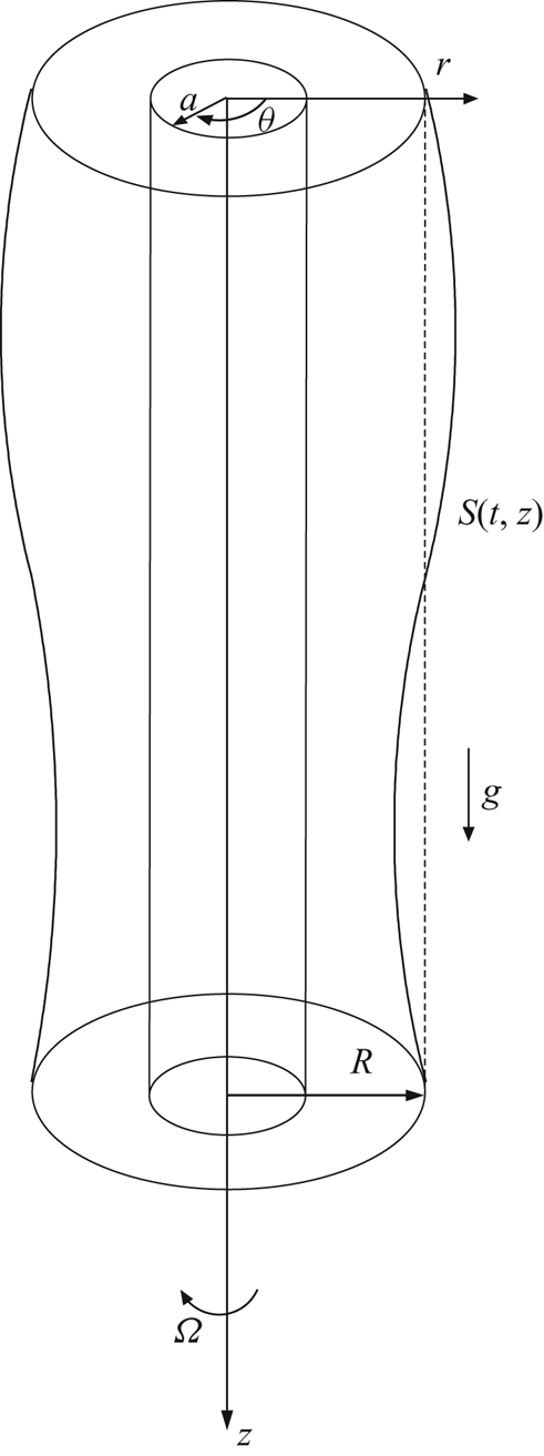
As shown in figure 1, a Newtonian fluid, of dynamic viscosity  $\mu$ and density $\rho$, flows down a vertical fibre of radius $r=a$ under gravity $g$. The cylinder rotates about its axis ( $z$-axis) at an angular speed $\Omega$. The initial radius of the fluid ring measured from the centre of the fibre is $r=R$. Let $(r, \theta , z)$ be the rotating cylindrical coordinates moving with the fibre.
Sketch of the geometry of a film flow coating a fibre.
The dynamics of the flow are governed by the Navier–Stokes equations,
 \begin{equation} \partial_{r}{u}+\frac{u}{r}+\frac{\partial_\theta v}{r}+\partial_{z}{w}=0, \end{equation}
 \begin{align} &\partial_t u+{u}\partial_r u+\frac{v}{r}\partial_\theta u+{w}\partial_z u-\frac{v^{2}}{r}\nonumber\\ &\quad =-\frac{\partial_r p}{\rho}+\Omega^{2} r-2\Omega v+\frac{\mu}{\rho}\left[\partial_{rr}u+\frac{\partial_r u}{r}+\frac{\partial_{\theta\theta}u}{r^{2}}+{\partial_{zz} u}-\frac{u}{r^{2}}-\frac{2}{r^{2}}\partial_\theta v\right], \end{align}
 \begin{align} & \partial_t v+{u}\partial_r v+\frac{v}{r}\partial_\theta v+{w}\partial_z v+\frac{uv}{r}\nonumber\\ &\quad =-\frac{1}{\rho}\frac{\partial_\theta p}{r}+2\Omega u+\frac{\mu}{\rho}\left[\partial_{rr}v+\frac{\partial_r v}{r}+\frac{\partial_{\theta\theta}v}{r^{2}}+{\partial_{zz} v}-\frac{v}{r^{2}}+\frac{2}{r^{2}}\partial_\theta u\right], \end{align}
 \begin{equation} \partial_t w+{u}\partial_r w+\frac{v}{r}\partial_\theta w+{w}\partial_z w=g-\frac{\partial_z p }{\rho}+\frac{\mu}{\rho}\left[\partial_{rr}w+\frac{\partial_r w}{r}+\frac{\partial_{\theta\theta}w}{r^{2}}+\partial_{zz}w\right], \end{equation}
in which  $p$ is the pressure and $\boldsymbol {u}$ is the velocity vector with $u$,
$u$,  $v$,
$v$,  $w$ denoting the components in $r$,
$r$,  $\theta$, $z$ directions. In the rotating coordinates, two additional forces, i.e. the centrifugal $\rho \Omega ^{2} r \boldsymbol {e}_r$ and Coriolis force $2\rho \Omega \boldsymbol {e}_z\times \boldsymbol {u}$, have been added as external forces in the governing equations.
At the fibre wall,  $r=a$, the velocity satisfies no-penetration and no-slip conditions
 \begin{equation} u=v=w=0. \end{equation}
At the free surface,  $r=S(\theta ,z,t)$, the balance of the normal stress is
 \begin{equation} \boldsymbol{n}\boldsymbol{\cdot}\boldsymbol{\mathsf{T}}\boldsymbol{\cdot}\boldsymbol{n}=2\sigma H, \end{equation}
where the surface tension,  $\sigma$, is constant. The balances of the shear stress are
 \begin{gather} \boldsymbol{t}_1\boldsymbol{\cdot}\boldsymbol{\mathsf{T}} \boldsymbol{\cdot}\boldsymbol{n}=0, \end{gather}
 \begin{gather} \boldsymbol{t}_2\boldsymbol{\cdot}\boldsymbol{\mathsf{T}} \boldsymbol{\cdot}\boldsymbol{n}=0, \end{gather}
where  $\boldsymbol{\mathsf{T}}$ is the stress tensor
 \begin{equation} \boldsymbol{\mathsf{T}} =\mu\left[ \boldsymbol{\nabla}\boldsymbol{u}+( \boldsymbol{\nabla}\boldsymbol{u})^{{\rm T}}\right], \end{equation} $\boldsymbol {t}_1$, $\boldsymbol {t}_2$ and $\boldsymbol {n}$ are the unit vectors tangential and normal to the interface
 \begin{gather} \boldsymbol{t}_1=\frac{\left(r^{-1}\partial_\theta S,1,0\right)}{\sqrt{1+r^{-2}(\partial_\theta S)^{2}}}, \end{gather}
 \begin{gather} \boldsymbol{t}_2=\frac{(\partial_z S,0,1)}{\sqrt{1+(\partial_z S)^{2}}}, \end{gather}
 \begin{gather} \boldsymbol{n}=\frac{(1,-r^{-1}\partial_\theta S,-\partial_z S)}{\sqrt{1+r^{-2}(\partial_\theta S)^{2}+(\partial_z S)^{2}}}, \end{gather}
and  $2H$ is the principal curvature of the surface
 \begin{equation} 2H=-\frac{1}{N}\left\{\frac{1}{S}+\frac{(\partial_\theta S)^{2}}{S^{3}}-\frac{\partial_{\theta\theta}S}{S^{2}}-\partial_{zz}S\right\}-\frac{1}{N^{2}}\left(\frac{\partial_\theta N \partial_\theta S}{S^{2}}+\partial_zS\partial_zN\right), \end{equation}
in which
 \begin{equation} N=\sqrt{1+r^{-2}(\partial_\theta S)^{2}+(\partial_z S)^{2}}. \end{equation}
The kinematic boundary condition on the free surface is
 \begin{equation} S_t+\frac{v}{r}\partial_\theta S+w\partial_z S=u, \end{equation}
or in conservative form
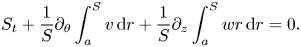 \begin{equation} S_t+\frac{1}{S}\partial_\theta \int_a^{S} v \,\textrm{d}r+\frac{1}{S}\partial_z \int_a^{S} wr \,\textrm{d}r=0. \end{equation}
2.1. Scalings
The non-dimensionalization is based on the viscous-gravity velocity,  $V\equiv \rho g R^{2}/\mu$, and the capillary length, $L=\sigma /\rho g R$. We assume that the radius of the fluid ring, $R$, is much smaller than the characteristic length $L$. The scalings are as follows:
 \begin{equation} \left.\begin{aligned} r=R r^{\ast},\ z=L z^{\ast},\ t=LV^{-1}t^{\ast},\ w=Vw^{\ast},\ u=\epsilon Vu^{\ast},\ v=\epsilon Vv^{\ast},\\ p=\rho g L p^{\ast},\ S=R S^{\ast},\ a=R a^{\ast},\quad\quad\quad\quad\quad\quad \end{aligned}\right\} \end{equation}
where the aspect ratio parameter  $\epsilon =R/L$ is a small number, and ‘ $\ast$’ denotes non-dimensional variables. Here, we assumed that the azimuthal velocity is also small, i.e. $v\sim O(\epsilon )$.
For convenience, we drop the  $\ast$ decoration and the dimensionless Navier–Stokes equations are expressed as
 \begin{equation} \partial_r u+\frac{u}{r}+\frac{1}{r}\partial_\theta v+\partial_z w=0, \end{equation}
 \begin{align}& \epsilon^{4} Re\left(\partial_t u+{u}\partial_r u+\frac{v}{r}\partial_\theta u+{w}\partial_z u-\frac{v^{2}}{r}\right)\nonumber\\ &\quad=-\partial_r p+\Omega_N r-2\epsilon\alpha\Omega_N v+ \epsilon^{2}\left[\partial_{rr}u+\frac{\partial_r u}{r}+\frac{1}{r^{2}}\partial_{\theta\theta}u-\frac{u}{r^{2}}+\epsilon^{2}{\partial_{zz} u}\right], \end{align}
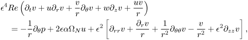 \begin{align} & \epsilon^{4} Re\left(\partial_t v+{u}\partial_r v+\frac{v}{r}\partial_\theta v+{w}\partial_z v+\frac{uv}{r}\right)\nonumber\\ &\quad=-\frac{1}{r}\partial_\theta p+2\epsilon\alpha\Omega_N u+ \epsilon^{2}\left[\partial_{rr}v+\frac{\partial_r v}{r}+\frac{1}{r^{2}}\partial_{\theta\theta}v-\frac{v}{r^{2}}+\epsilon^{2}{\partial_{zz} v}\right], \end{align}
 \begin{align} & \epsilon^{2} Re\left(\partial_t w+{u}\partial_r w+\frac{v}{r}\partial_\theta w+{w}\partial_z w\right)=1-\partial_z\,p + \partial_{rr}w+\frac{\partial_r w}{r}+\frac{1}{r^{2}}\partial_{\theta\theta}w+\epsilon^{2}\partial_{zz}w, \end{align}
where the Reynolds number is defined as  $Re=\rho V L/\mu$, and the parameters related to rotation are $\Omega _N=\Omega ^{2} R^{2}/g L$ and $\alpha =V/\Omega R$. This non-dimensionalization naturally results in $\epsilon =\rho g R^{2}/\sigma$, which is also referred to as the Bond number. The choice of small $\epsilon$ implies a small Bond number and surface-tension-dominated case. The full set of dimensionless parameters are $\epsilon$, $a$,
$a$,  $\Omega _N$, $\alpha$ and $Re$.
$Re$.
We choose the set of parameters used in the experiments by Kliakhandler etal. (Reference Kliakhandler, Davis and Bankoff2001), in which castor oil with density  $\rho =0.961 \times 10^{3}\ \textrm {kg}\,\textrm {m}^{-3}$, kinematic viscosity $\nu \equiv \mu /\rho =4.44 \times 10^{-4} \ \textrm {m}^{2}\,\textrm {s}^{-1}$, surface tension $\sigma =3.1\times 10^{-2} \ \textrm {kg}\,\textrm {s}^{-2}$, is used for coating. The radius of the fluid ring in initial state, $R$, is approximately $1\ \textrm {mm}$. For this set of physical parameters, the dimensionless parameter $\epsilon$ is less than 0.3 and the Reynolds number $Re\sim 10^{-2}$. We fixed the radius of the initial surface to be approximately $1\ \textrm {mm}$ and change the angular frequency of rotation $\Omega =2{\rm \pi} f$, in which $f$ is the frequency measured in cycles per second or Hertz. As $f$ changes in the range from 10 to 30 which is easily realized in experiments, $\Omega _N=0.1223$, 0.4890, 1.1003, $\alpha =0.3545$, 0.1772, 0.1182 for $f=10$, 20 and 30. When deriving the long-wave evolution equation, we assume the parameter $\Omega _N$ has order $O(1)$.
2.2. Linear stability
In the framework of normal mode analysis, the variables in the full Navier–Stokes equations are decomposed in the form of
 \begin{equation} [u,v,w,p,S]=[\bar{u},\bar{v},\bar{w},\bar{p},\bar{S}]+[\hat{u},\hat{v},\hat{w},\hat{p},\hat{S}]\exp[\textrm{i}(m\theta+kz-\omega t)], \end{equation}
in which ‘ $\bar {\ \ \ }$’, denotes the base state, ‘ $\hat {\ \ \ }$’, denotes the Fourier amplitudes of the disturbances, the integer $m$ and the real number $k$ denote the azimuthal and streamwise wavenumbers and $\omega$ denotes the frequency. The basic states of $u$,
$u$,  $w$ and $p$ are
 \begin{gather} \bar{u}=0, \end{gather}
 \begin{gather} \bar{w}=\frac{1}{4}(a^{2}-r^{2})+\frac{1}{2}\ln \frac{r}{a}, \end{gather}
 \begin{gather} \bar{p}=1+\frac{1}{2}\Omega_N(r^{2}-1). \end{gather}
The governing equations for the disturbances are as follows:
 \begin{equation} \texttt{D}\hat{u}+\frac{\hat{u}}{r}+\frac{\textrm{i}m}{r}\hat{v}+\textrm{i} k \hat{w}=0, \end{equation}
 \begin{align} & \epsilon^{4} Re(-\textrm{i}\omega \hat{u}+\textrm{i}k\bar{w} \hat{u})\nonumber\\ &\quad =-\texttt{D}\hat{p}-2\epsilon \alpha\Omega_N \hat{v} +\epsilon^{2}\left[\texttt{D}^{2} \hat{u} +\frac{\texttt{D}\hat{u}}{r}-\left(\epsilon^{2}k^{2}+\frac{m^{2}+1}{r^{2}}\right)\hat{u}-\frac{2\textrm{i}m\hat{v}}{r^{2}}\right], \end{align}
 \begin{align} &\epsilon^{4} Re(-\textrm{i}\omega \hat{v}+\textrm{i}k\bar{w} \hat{v})\nonumber\\ &\quad=-\frac{\textrm{i}m}{r}\hat{p}+2\epsilon \alpha \Omega_N \hat{u} +\epsilon^{2}\left[\texttt{D}^{2} \hat{v}+\frac{\texttt{D}\hat{v}}{r}-\left(\epsilon^{2}k^{2}+\frac{m^{2}+1}{r^{2}}\right)\hat{v}+\frac{2\textrm{i}m\hat{u}}{r^{2}}\right], \end{align}
 \begin{equation} \epsilon^{2} Re(-\textrm{i}\omega \hat{w}+ \texttt{D}\bar{w}\hat{u}+\textrm{i}k \bar{w}\hat{w})=-\textrm{i}k\hat{p}+\left[\texttt{D}^{2}\hat{w}+\frac{\texttt{D}\hat{w}}{r}-\left(\epsilon^{2}k^{2}+\frac{m^{2}}{r^{2}}\right)\hat{w}\right], \end{equation}
where  $\texttt {D}=\textrm {d}/\textrm {d}r$.
At the fibre wall ( $r=a$), the boundary conditions are
 \begin{equation} \hat{u}=\hat{v}=\hat{w}=0. \end{equation}
At the perturbed surface, boundary conditions are projected to  $r=1$ and after linearising, we have
 \begin{gather} \hat{p}-2\epsilon^{2}(\texttt{D} \hat{u}-\textrm{i}k\texttt{D} \bar{w} \hat{S})=-(1+\Omega_N\bar{S})\hat{S}+(m^{2}+\epsilon^{2} k^{2} )\hat{S}, \end{gather}
 \begin{gather} \texttt{D}\hat{w}+\texttt{D}^{2}\bar{w} \hat{S}+\textrm{i} \epsilon^{2} k \hat{u}=0, \end{gather}
 \begin{gather} r\texttt{D}\left(\frac{\hat{v}}{r}\right)+\frac{\textrm{i}m}{r}\hat{u}=0, \end{gather}
 \begin{gather} -\textrm{i} \omega \hat{S}+\textrm{i}k \bar{w}\hat{S}-\hat{u}=0. \end{gather}
The fully linearized Navier–Stokes equations are solved by a Chebyshev collocation method.
Figure 2 shows the dispersion relations of the axisymmetric mode ( $m=0$) and the non-axisymmetric mode ( $m=1$). At $f=0$, as shown in figure 2(a,d) for $a=0.3$ and 0.8, the axisymmetric mode is the most unstable. As $f=10$ in figure 2(b,e), the non-axisymmetric mode with $m=1$ becomes unstable in the long-wave range, but the maximum growth rate of $m=1$ is less than that of $m=0$. This indicates that the axisymmetric mode dominates the instability when the rotating speed is low. As $f$ increases to 20, as shown in figure 2(c,f) the asymmetric mode $m=1$ becomes the most unstable mode.
The curves of the dispersion relations predicted by the linearized Navier–Stokes equations (2.23)–(2.31) for ( $a) \ a=0.3$, $f=0$; ( $b) \ a=0.3$, $f=10$; ( $c) \ a=0.3$, $f=20$; ( $d) \ a=0.8$, $f=0$; ( $e) \ a=0.8$, $f=10$; ( $\,f) \ a=0.8$, $f=20$. Here, $f=0$ corresponds the non-rotating case of $\Omega _N=0$. At $f=10$ and $20$, the parameters related to rotation, $(\Omega _N, \alpha )$, are (0.1223, 0.3545) and (0.4890, 0.1772), respectively. The parameter $\epsilon \approx 0.3$.

In figure 3, we compare the dispersion relation of axisymmetric disturbances predicted by the fully linearized Navier–Stokes equations with that of neglecting the Coriolis forces, i.e. setting  $\alpha$ to be zero in (2.27) and (2.28). Figure 3 shows that the influence of the Coriolis forces on the stability is negligible when the rotating speed is low such that $\Omega _N\sim O(1)$. Therefore, in the following discussions, the Coriolis effect has been neglected.
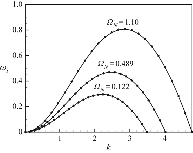
Comparison of the curves of the dispersion relations of axisymmetric modes with  $m=0$ predicted by the linearized Navier–Stokes equations (2.26)–(2.34) (solid lines) and the cases without Coriolis force (marked by solid circles). Other parameters are $a=0.3$, $\epsilon \approx 0.3$. The parameter $\Omega _N=0.122$, 0.489, 1.10 corresponds to $f=10$, 20, 30, respectively.
We will examine the nonlinear evolution of the most unstable mode for both low and high frequencies of rotation. At low frequency of rotation, the most unstable is axisymmetric, i.e. $m=0$. In this case, we derive an asymptotic model equation to describe the dynamics of the flow. In the fast rotation case, the results of the linear stability analysis have shown that the $m=0$ is not the most unstable. We should note that there exists different transitional routes in the present system, which depends on the initial conditions. When the rotation is slow, if the initial condition takes the non-axisymmetric form and has no streamwise component (the $m=0$ component), it can develop into a non-axisymmetric state because it is unstable. However, when the initial condition has a streamwise component, we observe fthat the final saturated state is axisymmetric, i.e. the non-axisymmetric mode is suppressed by the axisymmetric mode at small rotation number (see appendix B). When the rotation is fast, if we increase the rotation gradually and allow the axisymmetry mode to appear first, the non-axisymmetric mode $(m=1)$ will be bypassed, which has also been demonstrated by the simulation of a 3-D thin film model in appendix B. However, for a uniform film, if one suddenly rotates the cylinder at a high speed, the non-axisymmetric mode may appear first, which is confirmed by direct numerical simulation in appendices A and B. The axisymmetric state, however, might also be unstable to azimuthal disturbances, when the film is very thin. For example, Rietz etal. (Reference Rietz, Scheid, Gallaire, Kofman, Kneer and Rohlfs2017) observed that axisymmetric ring waves lose instability to a rivulet structure. A similar transitional scenario has also been found in a liquid film flowing underneath an inclined plane (Charogiannis etal. Reference Charogiannis, Denner, van Wachem, Kalliadasis, Scheid and Markides2018). It should be noted that the Rayleigh–Plateau mechanism is very weak and negligible in Rietz etal. (Reference Rietz, Scheid, Gallaire, Kofman, Kneer and Rohlfs2017) due to the small thickness of film. In the present work, both the Rayleigh–Plateau mechanism and the Rayleigh–Taylor instability are important because the film is thick. It will be very challenging to investigate the rivulet instability in the present case because deriving a simple model equation is not possible. However, the present axisymmetric model can be applied to understand the nonlinear wave dynamics on the crests of rivulets formed on the fibre, e.g. the interaction between different waves leading to an oscillating state.
2.3. A long-wave model
The linear stability analysis shows that the Coriolis effect is negligible at small rotation frequency,  $\Omega _N=O(1)$. The axisymmetric unstable mode dominates the primary instability when the rotating frequency is low $f\le 10$ and surface tension effect is dominant (small $\epsilon$). Assuming $\epsilon ^{2}\ll 1$, $Re\sim O(1)$ and slow rotation, we can neglect the inertial terms and the Coriolis force.
Under the assumption of axisymmetry, the leading-order Navier–Stokes equation is given by
 \begin{gather} 0=-\partial_r p+\Omega_N r, \end{gather}
 \begin{gather} \partial_{rr}w+\frac{\partial_r w}{r}=\partial_z p-1. \end{gather}
At the fibre wall  $r=a$,
 \begin{equation} w=0. \end{equation}
The leading-order tangential and normal stress balances at the surface ( $r=S$) are
 \begin{gather} \partial_r w=0, \end{gather}
 \begin{gather} p=\frac{1}{S}-\epsilon^{2} \partial_{zz}S. \end{gather}
It is notable that the term,  $\epsilon ^{2}S_{zz}$, which involves the highest derivative of $S$ is included in (2.39). In a linear analysis, the inclusion of this term is vital to give the correct cutoff wavenumber. Conventionally, this term is kept in long-wave theories of the problem with a cylindrical free surface, such as jets, threads and liquid bridges (Eggers & Dupont Reference Eggers and Dupont1994; Craster & Matar Reference Craster and Matar2006). An understandable explanation for the inclusion of this term is that the streamwise curvature is sufficiently large in some regions at the interface such as the steep front edge of a solitary hump. So, the term which contains the highest derivative of $S$ is sufficiently large and cannot be neglected even though it is multiplied by $\epsilon ^{2}$. For more justification of the inclusion of this term, we refer the reader to Craster & Matar (Reference Craster and Matar2006). An alternative choice is to keep the full curvature in the equation of the balance of the normal stresses in other related topics, for example, free-surface flows with large slopes (Snoeijer Reference Snoeijer2006) and rim or coating flows (Lopes, Thiele & Hazel Reference Lopes, Thiele and Hazel2018).
From (2.35) and (2.36), we obtain the pressure
 \begin{equation} p=\frac{1}{S}-\epsilon^{2} \partial_{zz}S+\frac{1}{2}\Omega_N(r^{2}-S^{2}), \end{equation}
and the velocity  $w(r,z,t)$
 \begin{equation} w=(1-\partial_z p)\left[\frac{1}{4}(a^{2}-r^{2})+\frac{1}{2}S^{2}\ln \frac{r}{a}\right]. \end{equation}
Substituting  $w$ into the kinematic boundary condition yields an evolution equation for $S(z,t)$ given by
 \begin{align} \partial_t S=-\frac{1}{16 S}\partial_z\left\{ \left(1+\frac{\partial_z S}{S^{2}}+\Omega_N S \partial_zS+\epsilon^{2} \partial_{zzz}S\right)\left[4S^{4}\log \frac{S}{a}+(3S^{2}-a^{2})(a^{2}-S^{2})\right]\right\}. \end{align}
Equation (2.42) is identical to Craster & Matar (Reference Craster and Matar2006) when the rotation is turned off.
2.4. Thin film limit
For the case in which the film is thin relative to the fibre, i.e.  $S(z,t)=a+h(z,t)$, where the film thickness $h\ll a$, expanding equation (2.42) for small $h$ results in the evolution equation for the thin film
 \begin{align} &\left(1+\frac{h}{a}\right)\partial_t h+\frac{1}{3}\frac{\partial}{\partial z}\nonumber\\
&\quad\times\left\{ h^{3}\left(1+\frac{h}{a}\right)\left[1+\frac{\partial_z h}{a^{2}(1+h/a)^{2}}+\Omega_Na(1+h/a)\partial_z h+\epsilon^{2} \partial_{zzz} h\right]\right\}=0. \end{align}
\begin{align} &\left(1+\frac{h}{a}\right)\partial_t h+\frac{1}{3}\frac{\partial}{\partial z}\nonumber\\
&\quad\times\left\{ h^{3}\left(1+\frac{h}{a}\right)\left[1+\frac{\partial_z h}{a^{2}(1+h/a)^{2}}+\Omega_Na(1+h/a)\partial_z h+\epsilon^{2} \partial_{zzz} h\right]\right\}=0. \end{align}
For very thin fluid films,  $a\rightarrow 1$ and $1+h/a\rightarrow 1$, the evolution equation can be further simplified as
 \begin{equation} \partial_t h+\frac{\partial}{\partial z}\left\{ \frac{h^{3}}{3}\left[1+(1+\Omega_N)\partial_z h+\epsilon^{2} \partial_{zzz} h\right]\right\}=0. \end{equation}
At  $\Omega _N=0$, (2.44) is reduced to the evolution equation of thin film by some authors (Frenkel Reference Frenkel1992; Kalliadasis & Chang Reference Kalliadasis and Chang1994). The roles of capillary forces and rotation on the stability of the film are manifested in (2.44). The terms $\partial _z h$, $\Omega _N \partial _z h$, $\epsilon ^{2} \partial _{zzz}h$ denote the contributions of azimuthal curvature, the rotation and the streamwise curvature, respectively. It is well known that the azimuthal curvature and the streamwise curvature are destabilizing and stabilizing, respectively (Kliakhandler etal. Reference Kliakhandler, Davis and Bankoff2001; Craster & Matar Reference Craster and Matar2006). From (2.44) for the thin film limit, it can be seen that the rotation is destabilizing the interface through the azimuthal curvature.
3. Linear stability analysis of the long-wave model
3.1. Dispersion relations
Let us now consider the linear stability of the problem. A small periodic disturbance in the streamwise direction is imposed on the film such that the film thickness can be decomposed into a base state component  $\bar {S}$, and a small disturbance of normal mode with amplitude $\hat {S}$,
 \begin{equation} S=\bar{S}+\hat{S}{\rm e}^{ \textrm{i}(kz-\omega t) }, \end{equation}
in which  $\omega$ is the complex frequency and $k$ is the wavenumber, and $\bar {S}=1$.
Substituting (3.1) into (2.42) yields the dispersion relation
 \begin{align} -\textrm{i}\omega+\left\{\frac{1}{16}k^{2}(k^{2}\epsilon^{2}-(1+\Omega_N)) \left(4 \ln \frac{1}{a}-a^{4}+4a^{2}-3\right)+\frac{\textrm{i}k}{2}(a^{2}-1-2\ln a) \right\}=0. \end{align}
At  $\Omega _N=0$, this dispersion relation is identical to that of Craster & Matar (Reference Craster and Matar2006) for a coating flow down a fibre. In the thin film limit as $a\rightarrow 1$, the dispersion relation corresponding to (2.44) tends to
 \begin{equation} -\textrm{i}\omega\sim \frac{1}{3}k^{2}[(1+\Omega_N)-k^{2}\epsilon^{2}] (1-a)^{3}-\textrm{i}k(1-a)^{2}. \end{equation}
We use  $\omega _r$ and $\omega _i$ to denote the real part and imaginary part of $\omega$. Here, $\omega _i$ and $\omega _r$ correspond to its growth or decay rate and the frequency of the disturbance. The phase speed of the disturbance is defined as $c={k}^{-1}{\omega _r}$. From (3.2), the phase speed
 \begin{equation} c=\frac{1}{2}(a^{2}-1-2\ln a), \end{equation}
is positive and independent of the wavenumber  $k$ and the rotation parameter $\Omega _N$. This means all disturbances with different wavenumbers propagate downstream at a same speed.
Craster & Matar (Reference Craster and Matar2006) have tested the validity of their model by comparing the results of the dispersion relation predicted by the long-wave model and the linear stability characteristics of the Stokes flow equations. The result showed that the model equation provides a reasonably good approximation of the full Navier–Stokes equations. In the present paper, we will test the validity of the model (2.42) with the presence of rotation. The details of the stability analysis of the full Navier–Stokes equations are presented in § 2.2. In order to know quantitatively the effect of rotation, in figure 4 we plot the curves of the dispersion relations (3.2) of the long-wave model and those via fully linear stability analysis.
Comparisons of the real growth rate of the axisymmetric mode  $m=0$ versus the wavenumber in the range of $0<k<k_c$ for various $\Omega _N$ between the stability analysis of the Navier–Stokes equations (solid lines) and the long-wave model (dashed lines). Other parameters are $\epsilon =0.2$, ( $a) \ a=0.5$, ( $b) \ a=0.9$.

We compared the dispersion relations for both models for two typical cases, thick film with  $a=0.5$ and thin film with $a=0.9$. Inspection of the dispersion curves indicates that the prediction of the long-wave model is in reasonable agreement with that predicted by the Navier–Stokes equations for various $\Omega _N$. For a fixed $k$, both models predict that the growth rate $\omega _i$ increases with the increase of $\Omega _N$. In figure 4(a), we observed that for thick film the time growth rate predicted by the long-wave model is obviously higher than that predicted by the linear stability analysis. However, in figure 4(b), the agreement between both models is excellent for the case of thin film.
3.2. Absolute and convective instabilities
For a general hydrodynamics stability problem, the wavenumber and frequency satisfy a dispersion relation in the form of
 \begin{equation} \mathcal{D}(k,\omega)=0. \end{equation}
In this subsection, we carry out a spatio-temporal stability analysis and both the wavenumber  $k$ and the frequency $\omega$ are complex numbers.
The stability properties of the perturbations are determined by the long-time behaviour of an impulsive response to a localized excitation. The solution of the impulsive response can be expressed in the form of
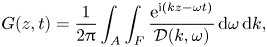 \begin{equation} G(z,t)=\frac{1}{2{\rm \pi}}\int_A\int_F\frac{{\rm e}^{\textrm{i}(kz-\omega t)}}{\mathcal{D}(k,\omega)}\,\textrm{d}\omega\,\textrm{d}k, \end{equation}
where the Bromwich contour  $F$ in the $\omega$-plane is a horizontal line lying above all the singularities to satisfy causality, and the integration path $A$ lies inside the analyticity band around the $k$-axis.
The nature of CI and AI can be identified by examining the long-time behaviour of the wavenumber  $k_0$ along the ray $z/t$ at a fixed spatial location. This complex $k_0$ has, by definition, a zero group velocity
 \begin{equation} \frac{\partial \omega}{\partial k}(k_0)=0, \end{equation}
and  $\omega _0=\omega (k_0)$ is called the absolute frequency. If ${\rm Im} (\omega _0)>0$/ ${\rm Im} (\omega _0)<0$, the flow is said to be absolutely/convectively unstable. It should be noted that the saddle point $k_0$ must be identified by the Briggs–Bers collision criterion (Briggs Reference Briggs1964; Bers Reference Bers, DeWitt and Peyraud1975), i.e. the saddle point must be a pinch point produced by the collision of two distinct spatial branches of solutions coming from the upper and lower half- $k$-planes. In the pinching process, when $\omega$ moves from above along the vertical line down to $\omega _0$, the two spatial branches $k_1(\omega )$ and $k_2(\omega )$ originate in this movement on opposite sides of the real $k$-axis and collide at $k=k_0$ and $\omega =\omega _0$. For more details on the topics related to AI–CI problems, we refer the reader to a good review article by Huerre & Monkewitz (Reference Huerre and Monkewitz1990). The most relevant work to the present problem is the study on the AI–CI characteristics of an exterior coating film down a vertical fibre (Duprat etal. Reference Duprat, Ruyer-Quil, Kalliadasis and Giorgiutti-Dauphiné2007). Very recently, an experimental study by Sadeghpour etal. (Reference Sadeghpour, Zeng, Ji, Ebrahimi, Bertozzi and Ju2019) also showed that the water–vapour transfer rate in the coating flow is dependent on the AI–CI characteristics. For example, when the flow is absolutely unstable, the water–vapour transfer rate is generally promoted by increasing the liquid flow rate. However, in the convectively unstable situation, the water–vapour transfer rate does not increase with the liquid flow rate due to the occurrence of irregular beads.
From the dispersion relation, (3.2), the complex frequency  $\omega$ can be expressed as a polynomial of $k$:
$k$:
 \begin{equation} \omega=\frac{\textrm{i}}{16} k^{2}[(1+\Omega_N)-\epsilon^{2}k^{2}]\,f_1+k f_2, \end{equation}
in which
 \begin{gather} f_1=4 \ln \frac{1}{a}-a^{4}+4a^{2}-3, \end{gather}
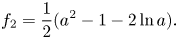 \begin{gather} f_2=\frac{1}{2}(a^{2}-1-2\ln a). \end{gather}
Through the transformation  $k=\alpha \tilde {k}$, $\beta =(1+\Omega _N)(\alpha \epsilon )^{-2}$, $\tilde {\omega }=\omega (\alpha f_2)^{-1}$, where $\alpha =[(16f_2)/(3f_1 \epsilon ^{2})]^{1/3}$, the dispersion relation reduces to a standard form as
 \begin{equation} \tilde{\omega}=\tilde{k}+\frac{\textrm{i}\tilde{k}^{2}}{3}({\beta}-\tilde{k}^{2}). \end{equation}
A straightforward analysis based on (3.11) then shows that the instability becomes absolute when  ${\beta }>{\beta }_c= [(9/4)(-17+7\sqrt {7})]^{1/3}\approx 1.5$ (Duprat etal. Reference Duprat, Ruyer-Quil, Kalliadasis and Giorgiutti-Dauphiné2007). Therefore, applying $\beta =(1+\Omega _N)(\alpha \epsilon )^{-2}$ to the condition ${\beta }>{\beta }_c$ yields the following implicit condition for absolute instability:
 \begin{equation} (1+\Omega_N)\left(\frac{3f_1}{16 \epsilon f_2 }\right)^{2/3}>{\beta}_c . \end{equation}
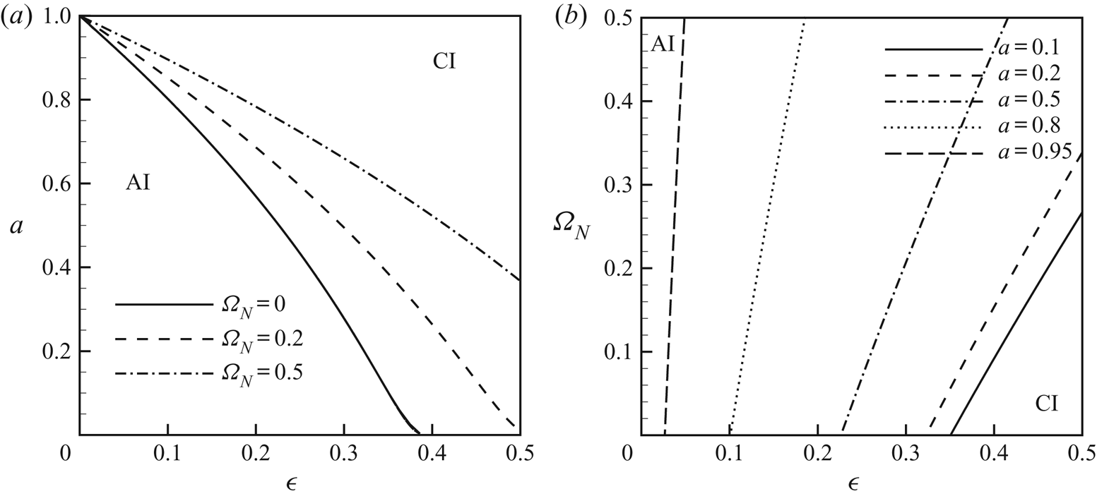
 In figure 5(a,b), we present the AI–CI boundaries for various  $\Omega _N$ in the $\epsilon\hbox{--}a$ plane and for various $a$ in the $\epsilon\hbox{--}\Omega _N$ plane, respectively. The range of parameter $a$ is ( $0,1$). The model is valid for small $\epsilon$, however, when presenting the results we extend the range of $\epsilon$ to 0.5. As shown in figure 5(a), for each curve with the decrease of $a$ or $\epsilon$ the flow regime can switch from convective instability to absolute instability. With the increase of $\Omega _N$, the absolutely unstable regime extends in the $\epsilon\hbox{--}a$ plane. In figure 5(a), as $\Omega _N=0$ the convective regime occupies a large portion of area in the $\epsilon\hbox{--}a$ plane. With the increase of $\Omega _N$, some CI regimes become absolutely unstable and the boundary extends counterclockwise in the $\epsilon\hbox{--}a$ plane. In figure 5(b), it is shown that for each value of $a$ with the increase of $\Omega _N$ the flow switches from the CI to the AI regime. The results of figure 5 indicate that the increase of rotation promotes the absolute instability.
The boundaries between CI and AI, ( $a$) in the $\epsilon\hbox{--}a$ plane for various $\Omega _N$, ( $b$) in the $\epsilon\hbox{--}\Omega _N$ plane for various $a$.
$a$.
4. Nonlinear evolutions
In this section, we will study the nonlinear evolution from the initial state seeded with small disturbances. Equation (2.42) subject to periodic boundary conditions was solved numerically using a Fourier spectral method. The solution of  $S(z,t)$ is expanded by the Fourier series
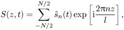 \begin{equation} S(z,t)=\sum_{-N/2}^{N/2}\hat{s}_n(t)\exp\left[\textrm{i}\frac{ 2{\rm \pi} n z}{l}\right], \end{equation}
in which  $N$ is the number of Fourier modes, $\hat {s}_n(t)$ is the time-dependent coefficient and $l$ is the computational length. A Fourier collocation is used to provide the discretization in space for periodic problem. We employed an implicit Gear's method for stiff problems for the time stepping and the relative error is $10^{-6}$ at each time step (Ding & Willis Reference Ding and Willis2019).
4.1. AI–CI instability
In this subsection, we performed numerical simulations on the nonlinear evolution of (2.42) to examine the effect of rotation on the transition from CI to AI regimes. We choose the set of parameters of  $a=0.3$ and $\epsilon =0.4$ which lies in the CI regime for $\Omega _N=0$ and in the AI regime for $\Omega _N=0.5$. The initial condition is seeded with $S(z,0)=0.1 \exp [-(z -20)^{2}/{2}]$ and the length of computational domain $l=100$.
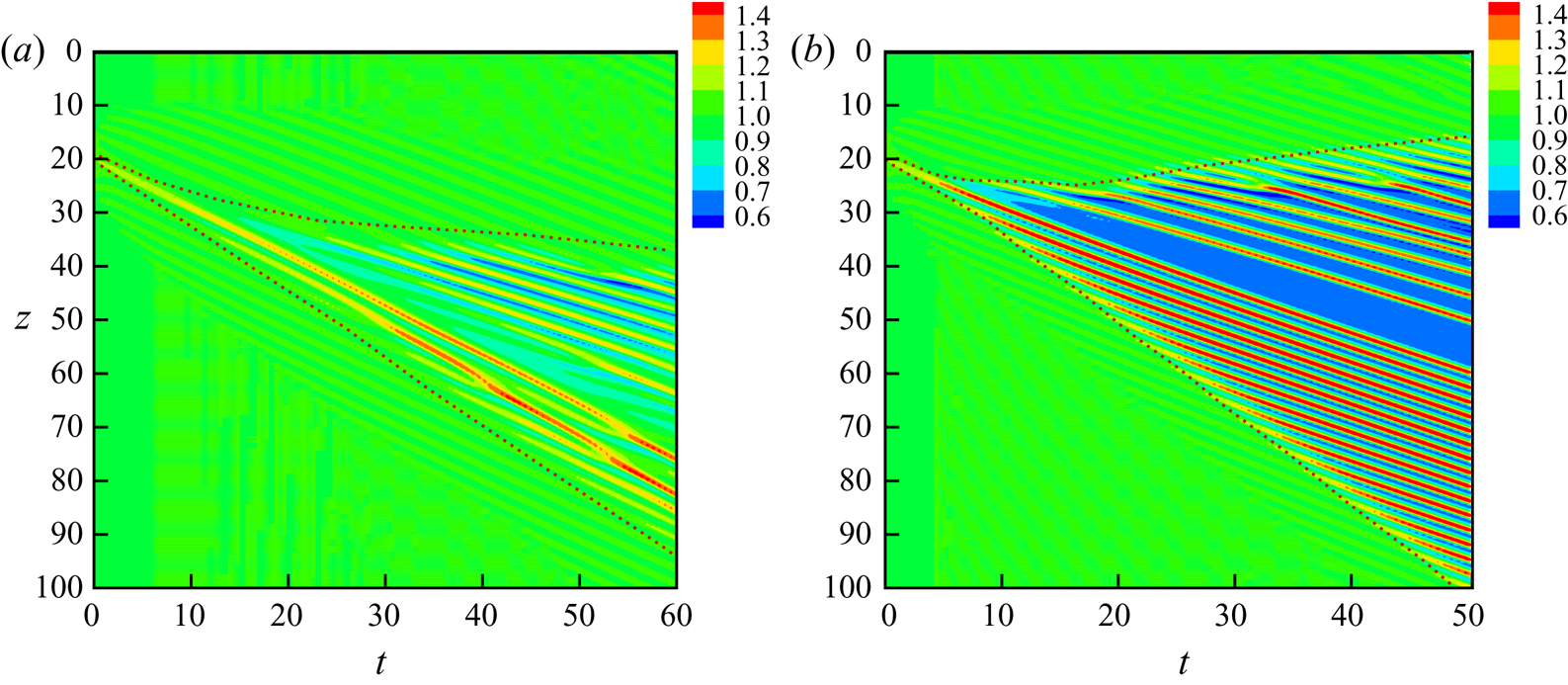
In figure 6, we present the spatio-temporal diagram for various  $\Omega _N$, which may be helpful for us to understand the effect of rotation on the AI–CI characteristics. For $\Omega _N=0$, the flow is linearly convectively unstable. In figure 6(a) it is obvious that the disturbance propagates downstream and decays at $z=20$. As $\Omega _N$ increases to 0.5, as shown in figure 5, the flow is absolutely unstable as the point of (0.4, 0.3) in the $\epsilon\hbox{--}a$ plane is below the AI–CI boundary of $\Omega _N=0.5$. In figure 6(b), as $\Omega _N=0.5$, the flow becomes absolutely unstable as the disturbance is amplified both downstream and upstream.
Spatial-temporal diagram for  $a=0.3$, $\epsilon =0.4$. The values of $S(z,t)$ are marked by different colours. ( $a) \ \Omega _N=0$; ( $b) \ \Omega _N=0.5$.
4.2. Transient simulations in long domains
In order to know the properties of the solutions which are naturally selected, we performed numerical simulations in long domains subject to a pseudo-random initial condition. Two typical sets of parameters of  $a$ and $\epsilon$ are chosen. Kliakhandler etal. (Reference Kliakhandler, Davis and Bankoff2001) and Craster & Matar (Reference Craster and Matar2006) have performed simulations on the nonlinear evolution for three regimes in Kliakhandler etal. (Reference Kliakhandler, Davis and Bankoff2001) and all of them are in the absolute instability regime. The first set of parameters, $a=0.255$ and $\epsilon =0.292$ chosen in this paper, which falls in the absolute instability regime, is identical to that used by Kliakhandler etal. (Reference Kliakhandler, Davis and Bankoff2001) and Craster & Matar (Reference Craster and Matar2006). The second set of parameters, $a=0.55$ and $\epsilon =0.3$, however, is picked from the convectively unstable regime when $\Omega _N=0$, which becomes absolutely unstable when $\Omega _N>0.2$.
The system becomes saturated after long-time evolution. In figure 7, we present the results of the first set of parameters, which is in the absolutely unstable regime. In figure 7(a–d), similar-sized large droplets are moving as a bound state. The heights of these droplets are very close but the gaps between them can vary. The increase of  $\Omega _N$ leads to the formation of more pronounced and closely spaced beads with smaller sizes. Moreover, the gaps between different beads become flatter and thinner.
The profiles of the interface via transient numerical simulations for various  $\Omega _N$. Other parameters are $a = 0.2551$, $\epsilon = 0.2915$. The instant time is $t=100$. The coordinate $\zeta =z/\epsilon$. Here, $\Omega _N=0$, 0.2, 0.5 for ( $a$), ( $b$) and ( $c$), respectively.
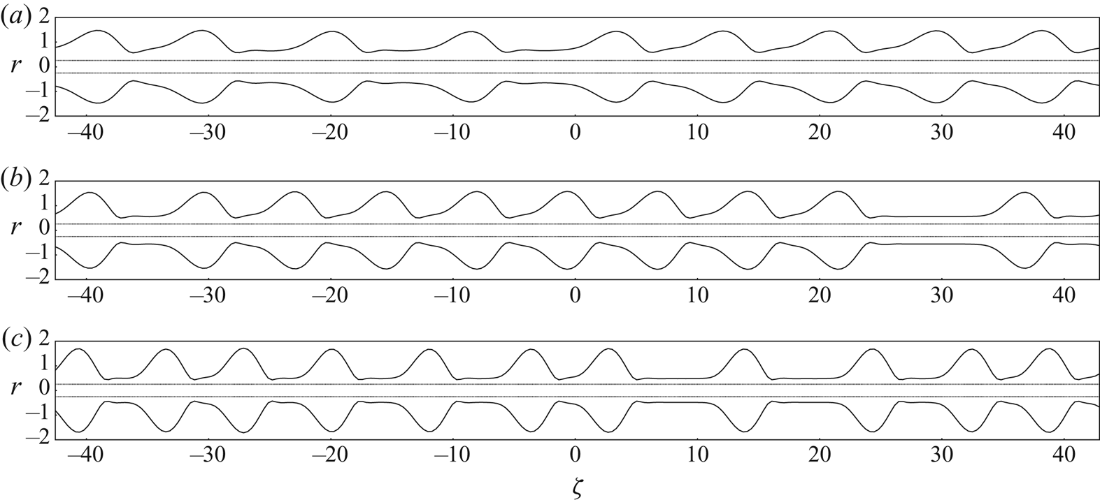
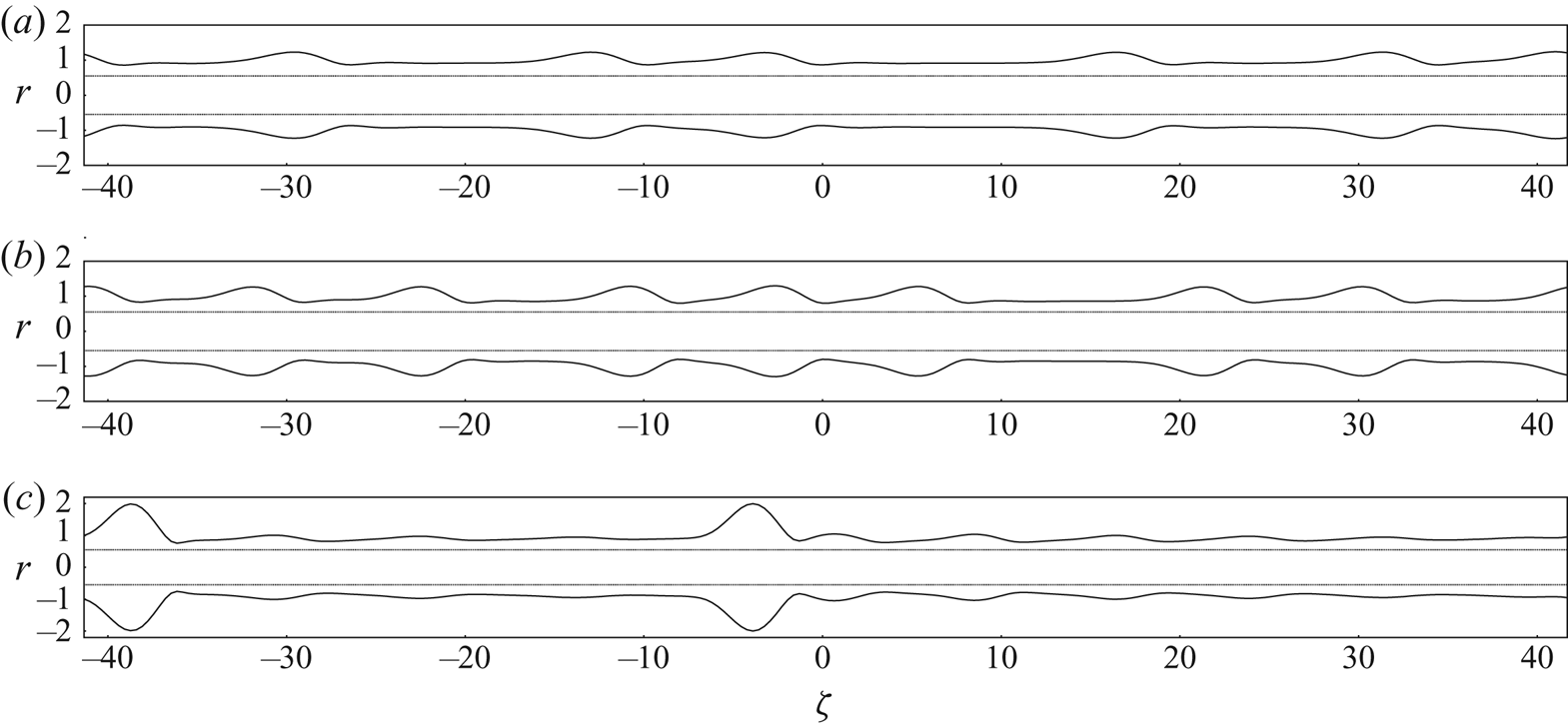
Figure 8 shows the film profiles for different values of  $\Omega _N$, which demonstrates that the rotation has a significant influence on the flow pattern. In these figures, the height of the beads increases with the increase of $\Omega _N$. Comparing with figure 8(a,c), in which $\Omega _N$ increases from $\Omega _N=0$ to $\Omega _N=0.5$, the height of the beads in figure 8(c) is obviously larger than that in figure 8(a). However, the large droplet numbers are reduced from six to two. Hence, the gap between the large drops in figure 8(c) is much longer than that in figure 8(a). This long film between the two large droplets in figure 8(c) is unstable and breaks into several tiny beads. The large droplet, however, will catch up with and consume these small beads ahead and leave behind a flat film where small beads will regenerate again.
The profiles of the interface via transient numerical simulations for various  $\Omega _N$. Other parameters $a = 0.55$, $\epsilon = 0.3$. The instant time is $t=500$. The coordinate $\zeta =z/\epsilon$. Here, $\Omega _N=0$, 0.2, 0.5 for $(a),(b),(c)$, respectively.
5. Travelling-wave solutions and their stabilities
5.1. Travelling-wave solutions
Experiments have shown different types of steadily propagating solutions in the form of highly organized droplets or bead-like solutions separated by long space (Kliakhandler etal. Reference Kliakhandler, Davis and Bankoff2001). In this subsection, we will examine how rotation influences the characteristics of these steady travelling-wave solutions.
We solve the governing equations by moving to a travelling-wave coordinate. In the moving system, it is convenient to define
 \begin{gather} \tau=t, \end{gather}
 \begin{gather} \xi=z-ct, \end{gather}
where  $c$ is the wave speed of the moving coordinate. The derivatives with respective to $t$ and $z$ can be expressed as
 \begin{gather} \partial_t=\partial_\tau-c\partial_\xi, \end{gather}
 \begin{gather} \partial_z=\partial_\xi. \end{gather}
For a travelling-wave solution, the time derivation of  $S$ with respect to $\tau$ is zero, and the profile of the interface has the form of $S=S(\xi )$. The nonlinear equation (2.42) becomes
 \begin{equation} -c\partial_\xi S^{2}+2\partial_\xi Q(S)=0, \end{equation}
where
 \begin{equation} Q(S)=\frac{1}{16}\left(1+\frac{\partial_\xi S}{S^{2}}+\Omega_N S \partial_\xi S+\epsilon^{2} \partial_{\xi\xi\xi}S\right)\left[4S^{4}\log \frac{S}{a}+(3S^{2}-a^{2})(a^{2}-S^{2})\right]. \end{equation}
Integrating equation (5.5) once, we have
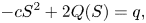 \begin{equation} -c S^{2}+2 Q(S)=q, \end{equation}
where  $q$ is an integral constant. Equation (5.7) subject to periodic boundary conditions will be solved in the region of $-l/2<\xi \leq l/2$, where the length of the computational domain, $l$, is the wavelength of the travelling-wave solution. To fix $c$, we impose the mass conservative condition
 \begin{equation} \int_{-l/2}^{l/2}(S^{2}(\xi)-a^{2})\,\textrm{d}\xi=l(1-a^{2}). \end{equation}
To break the translational symmetry, one can enforce the real (or imaginary) part of the first Fourier mode to zero such that  $q$ can be determined. A code for Newton iteration based on Ding & Willis (Reference Ding and Willis2019) was developed to solve the present problem. The solution can be tracked from the Hopf bifurcation point ( $\omega _i=0$) with branch continuation.
Typical profiles of the travelling-wave solutions are shown in figure 9. As shown in figure 9, the droplet height is increased by the axial rotation. In Craster & Matar (Reference Craster and Matar2006) and Ding & Willis (Reference Ding and Willis2019), an observation is that higher droplets are moving faster than lower droplets. However, in the present study, it is found that this conclusion holds only if the axial rotation is slow (see figure 10a, in which the wave speed  $c$ increases with $\Omega _N$). When the rotation becomes fast ( $\Omega _N>0.5$), we observe that large droplets can move slower than small droplets (see figure 10b), which is contrary to the conclusions of Craster& Matar (Reference Craster and Matar2006) and Ding & Willis (Reference Ding and Willis2019).
Interface profile for the travelling-wave solution for various  $\Omega _N$. Other parameters are $\epsilon = 0.2$ and $a=0.25$. ( $a) \ l=2$; ( $b) \ l=6$.
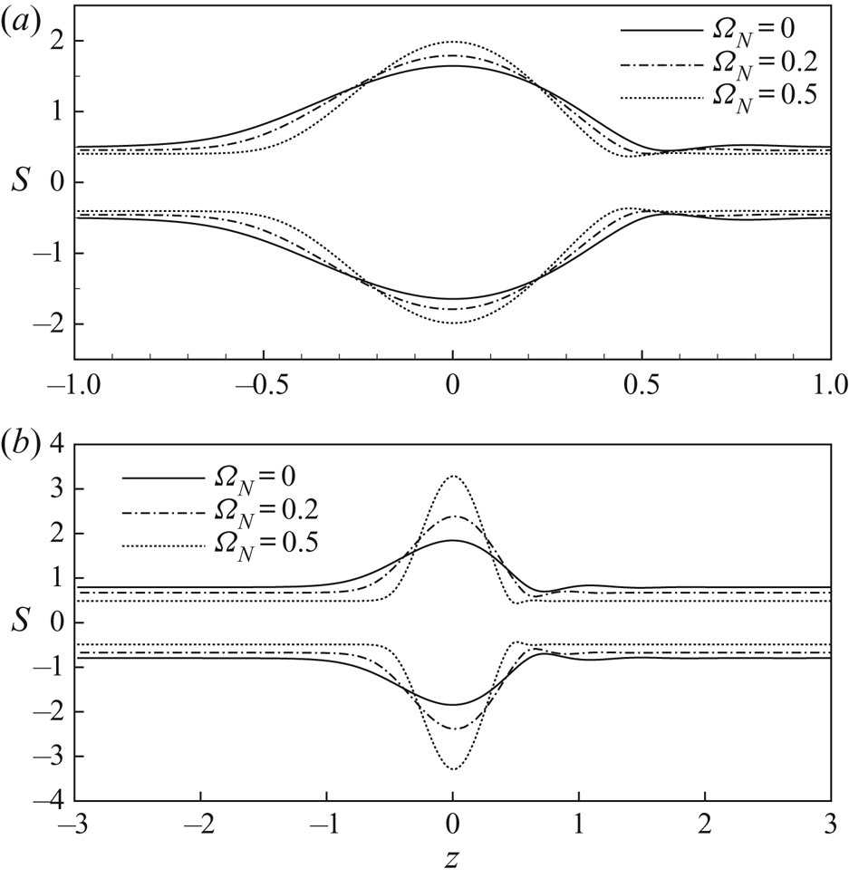
Travelling-wave solution for one-hump solutions: spacings  $l$ and propagating speeds $c$ for various $\Omega _N$ at $\epsilon = 0.2$ and $a=0.25$.
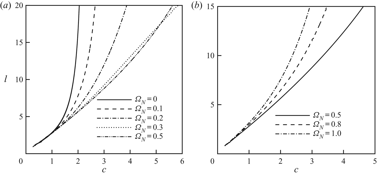
To account for the physical mechanism of the abnormal phenomenon, we plot the flow field in figure 11 in the moving frame. It indicates that the reversal flow in the wave hump becomes stronger as  $\Omega _N$ increases. This reversal flow can significantly increase the viscous dissipation effect. In their work, Ruyer-Quil etal. (Reference Ruyer-Quil, Treveleyan, Giorgiutti-Dauphiné, Dupat and Kalliadasis2008) derived a weighted residual model, which considered the streamwise dissipation effect, and they found that the wave speed of the travelling-wave solution in flow regime ‘c’ is lower than Craster & Matar (Reference Craster and Matar2006). As also discussed by Ding & Willis (Reference Ding and Willis2019) that viscous dissipation effect can slow the droplet motion, it is suggestive that the motion of large droplets is retarded by this strong reversal flow in the hump.
The flow field in the moving frame at  $\Omega _N=0.5,\,0.8,\,1$ for ( $a$), ( $b$) and ( $c$), respectively.
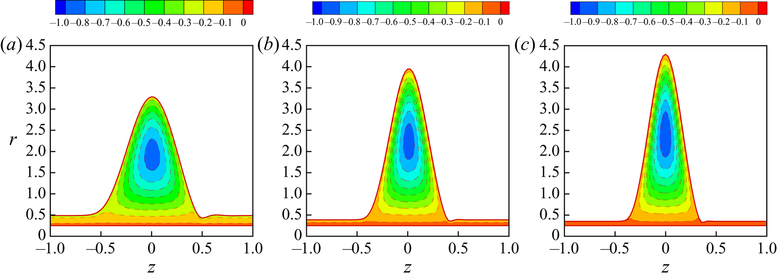
5.2. Stability of the travelling-wave solution
Numerical simulations of the present problem showed that not all the travelling waves can be obtained through the evolution of an initial condition. It is natural to examine whether the travelling-wave solutions with different wavelengths are stable.
We performed a linear stability analysis on the travelling-wave solutions in the moving frame at the wave speed  $c$. The profile of the interface is the travelling-wave solutions perturbed by an infinitesimal disturbance
 \begin{equation} S(\xi,\tau)=\bar{S}(\xi)+S'(\xi,\tau), \end{equation}
in which  $S'(\xi ,\tau )=\hat {S}(\xi ){\rm e}^{-\textrm {i}\omega \tau }$.
The linearized evolution equation is written as
 \begin{equation} \bar{S}\partial_\tau S'-c\partial_\xi(\bar{S}S')+\partial_\xi\{(1-\partial_\xi \bar{p})\mathcal{F}_S S'-{\mathcal{F}}\partial_\xi p'\}=0, \end{equation}
in which
 \begin{gather} \partial_\xi \bar{p}=-\frac{\bar{S}_\xi}{\bar{S}^{2}}-\epsilon^{2}\partial_{\xi\xi\xi}\bar{S}-\Omega_N \bar{S} \partial_\xi\bar{S}, \end{gather}
 \begin{gather} \partial_\xi p'=-\frac{\partial_\xi S'}{\bar{S}^{2}}+2\partial_\xi\bar{S}\frac{S'}{\bar{S}^{3}}-\epsilon^{2} \partial_{\xi\xi\xi}S'-\Omega_N(\bar{S}\partial_\xi S'+\partial_\xi \bar{S}S'), \end{gather}
 \begin{gather} \mathcal{F}_S=\bar{S}^{3}\ln \frac{\bar{S}}{a} +\frac{\bar{S}(a^{2}-\bar{S}^{2})}{2}, \end{gather}
 \begin{gather} \mathcal{F}=\frac{\bar{S}^{4}}{4}\ln \frac{\bar{S}}{a} +\frac{(3\bar{S}^{2}-a^{2})(a^{2}-\bar{S}^{2})}{16}. \end{gather}
 The curves of the leading eigenvalue of the travelling-wave solutions versus the wavelength are shown in figure 12. For  $\Omega _N=0$, there exists a critical wavelength $l_c\approx 3.5$ beyond which the travelling-wave solutions are unstable. As $l >l_c$, a conjugate complex pair of eigenvalues are found. In figure 12(a), the curves of the growth rate consists of several segments, indicating that mode switching occurs as $l$ increases. This is also reflected by the non-continuous curves of temporal frequency $\omega _r$ as shown in figure 12(b). As shown in figure 12(a), with the increase of $\Omega _N$ the critical wavelength $l_c$ increases. As $\Omega _N$ increases from 0 to 0.2, the growth rate decreases as $l<12$ and increases as $l>12$. As $\Omega _N$ increases from 0.2 to 0.6, the effect of rotation is stabilizing. In figure 12(a), for $\Omega _N=0.6$ the unstable region is confined in a limited band of $l$. When $\Omega _N$ increases further, the travelling-wave solutions become completely stable. In figure 12(b), the frequency of the most unstable mode increases with the increase of $\Omega _N$. The results in figure 12 showed that the effect of rotation on the travelling-wave solution is adverse to the linear stability of the trivial base state $\bar {S}=1$ in which the rotation is destabilizing.
The curves of the leading eigenvalue for the travelling-wave solutions versus the wave length  $l$. ( $a$) The time growth rate $\omega _i$, ( $b$) the frequency $\omega _r$. Other parameters are $\epsilon = 0.2$ and $a=0.25$.

It is interesting to examine the structures of the most unstable mode of different segments in figure 12(a). In figure 13, the profiles of the most unstable mode are plotted for two typical sets of parameters. The structures of the disturbances are similar in these two figures. The disturbance consists of a series of ripples occupying the whole spatial domain. The disturbed surface is in the form of a large bead accompanied by a series of smaller beads. We also examine the structures of the most unstable mode for various parameters of  $l$ and $\Omega _N$. The results of the linear stability analysis indicate that the structures of different segments are similar. The slight difference is that the numbers of small ripples may increase with $l$. It is obvious that the profiles in figure 13 provide initial states involving the interaction between a large bead and several smaller ones.
The profile of the leading unstable mode with  $L=5$. ( $a) \ \Omega _N=0$; ( $b) \ \Omega _N=0.4$. The dashed line denotes the basic state. Other parameters are $\epsilon = 0.2$ and $a=0.25$.
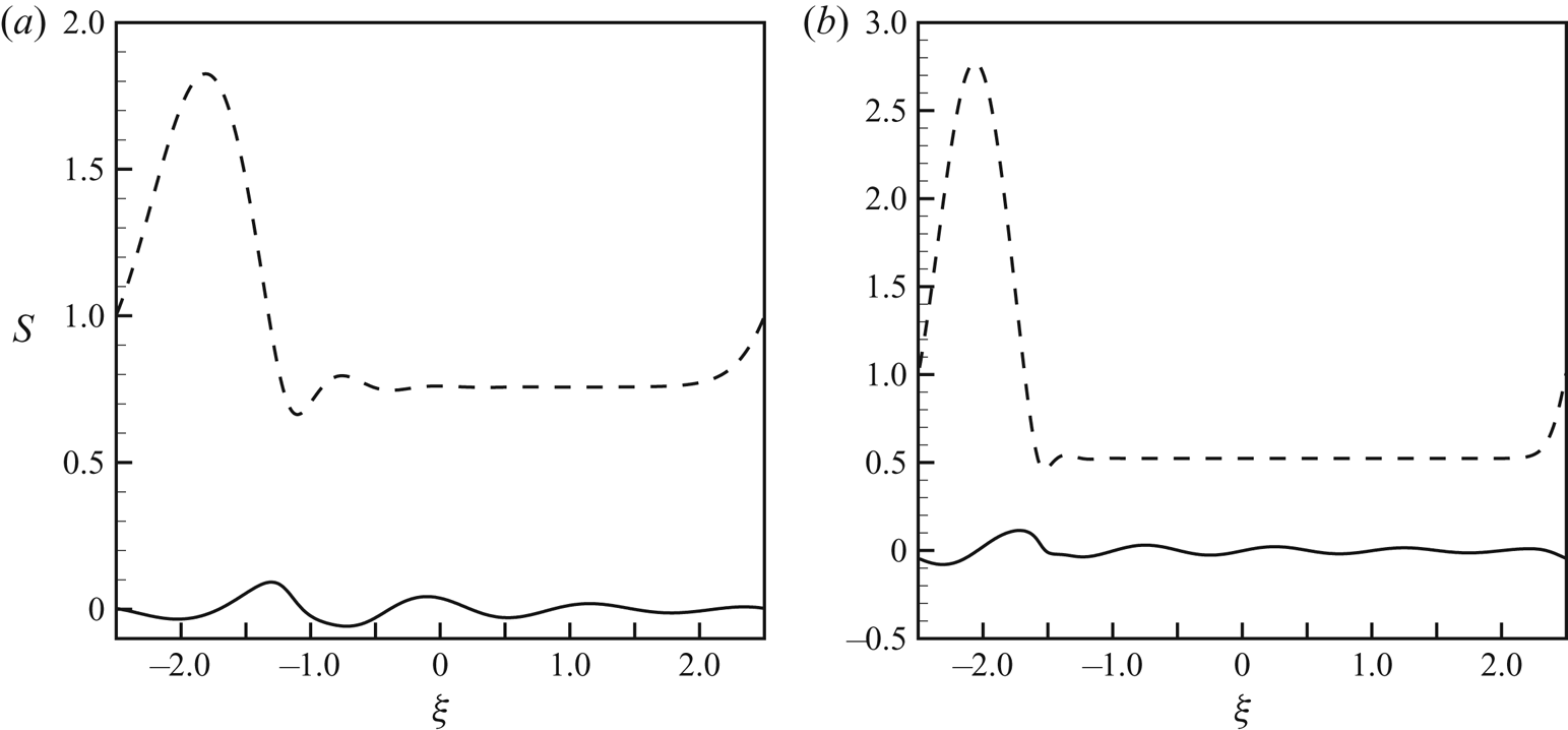
In the experiments by Kliakhandler etal. (Reference Kliakhandler, Davis and Bankoff2001), the flow regime ‘c’ presents dynamic behaviours different from the steady travelling waves, in which a complicated interaction between a large droplet and several small droplets causes an oscillatory flow. It is interesting to investigate how the rotation influences the dynamics of the oscillatory flow, i.e. flow regime ‘c’. To answer this question, we perform numerical simulations on the evolution initiated by a travelling-wave solution superposed of the most unstable mode. Before we study the nonlinear evolution by numerical simulations, it is helpful to discuss the nature of the stability of travelling-wave solutions. We classify the stability of travelling-wave solutions as being either convectively unstable or absolutely unstable. If the travelling-wave solutions are convectively unstable, they can tolerate localized disturbances and the flow ultimately evolves into a state in which the travelling waves interact with small ripples. If the travelling-wave solutions are absolutely unstable, these solutions can be destroyed by localized disturbances and evolve into a new state after a long time of evolution. As discussed in figure 13, the eigenvalues corresponding to the most unstable modes are in the form of a pair of conjugated complex numbers. This means the most unstable mode is convectively unstable and can escape the travelling wave downstream or upstream. For related discussion on the stability of a two-dimensional pulse on electrified falling films, see Blyth etal. (Reference Blyth, Tseluiko, Lin and Kalliadasis2018).
In figure 14, the space–time diagrams of a long-time evolution are plotted for several typical cases. In figure 14(a) for  $l=4$ and $\Omega _N=0$ in which the travelling-wave solution is unstable as shown in figure 12, the oscillatory behaviour of the height of the large droplets is obvious. In this space–time diagram, it is observed that the oscillation is both temporally and spatially periodic. In figure 14(b) for $l=4$ and $\Omega _N=0.4$, there is no oscillation in the space–time diagram, indicating the system is a steady travelling wave. In figure 14(c,d), the space–time diagrams are plotted for two typical cases with $l=7$ in which the travelling-wave solutions are unstable. The characteristics of the structures in figure 14(a,c,d) are qualitatively similar. In these figures, smaller ripples arrange periodically in the $z\hbox{--}t$ plane, and the loci of the large droplets oscillate periodically. The flow can be considered as an oscillatory travelling wave, which conforms to the fact that the travelling-wave solutions are convectively unstable. The numerical simulations suggest that the time-periodic state is a relative periodic orbit (RPO), which has been reported by Ding & Willis (Reference Ding and Willis2019) in a non-rotating system. However, it is unclear how the rotation affects the mean speed and the period of the RPO. We will proceed to § 5.3 to answer this question.
The space–time diagrams for the travelling waves perturbed by the most unstable mode. The contours of  $S(z,t)$ are marked by different colours. $(a)\ L=4$, $\Omega _N=0$; $(b)\ L=4$, $\Omega _N=0.4$; $(c)\ L=7$, $\Omega_N=0.2$; $(d)L=7$, $\Omega _N=0.4$. Other parameters are $\epsilon = 0.2$ and $a=0.25$.
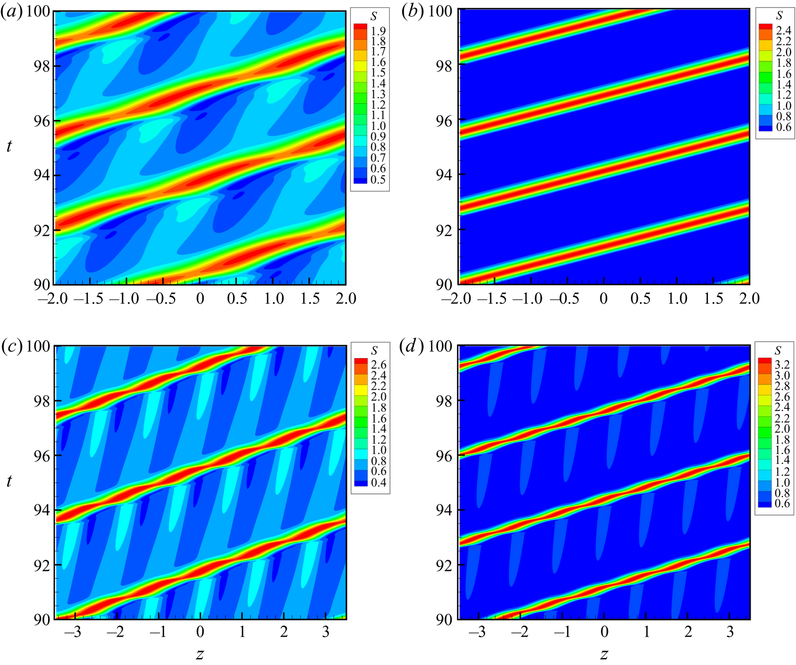
5.3. Exact RPOs
To find the exact RPOs of the present problem, we search for the recurrent solutions in the system
 \begin{equation} S(z,t)=S(z+s,t+T), \end{equation}
where  $s$ is the spatial shift along the axis of the fibre and $T$ is the time period. Each RPO has its own particular period $T$, while a travelling wave has arbitrary period $T$. Given an initial guess of $\boldsymbol {X}_0=[S_0,s_0,T_0]^{\textrm {T}}$, we can obtain a better guess $\boldsymbol {X}_0+\delta \boldsymbol {X}_0$ by solving
 \begin{equation} \frac{\partial \boldsymbol{F}}{\partial S_0}\delta S_0+ \frac{\partial \boldsymbol{F}}{\partial s}\delta s+ \frac{\partial \boldsymbol{F}}{\partial T}\delta T=-\boldsymbol{F}, \end{equation}
where  $\boldsymbol {F}=S(z+s,t+T)-S_0$. The solution $S_0$ is approximated by a Fourier expansion of $2N$ modes. Plus two other unknown parameters $T$ and $s$, there are $2N+2$ unknowns. To close the system, we require the update $\delta \boldsymbol {X}_0$ has no component in the $z$ direction and the $t$ direction (Ding & Willis Reference Ding and Willis2019):
 \begin{gather} \frac{\partial S^{T}_0}{\partial z}\delta S_0 =0, \end{gather}
 \begin{gather} \frac{\partial S^{T}_0}{\partial t}\delta S_0 =0. \end{gather}
Equation (5.16) and the two constraints constitute the following linear algebra problem:
 \begin{equation} \boldsymbol{A} \delta \boldsymbol{X}=\boldsymbol{b}, \end{equation}
where  $\boldsymbol {b}=[\boldsymbol {F},0,0]^{\textrm {T}}$. It is impossible to write down the explicit Jacobian $\boldsymbol {A}$ but an alternative way to solve this problem is to work in the Krylov subspace spanned by $\mathcal{K}_n=\{\boldsymbol {b},\boldsymbol {A}\boldsymbol {b},\boldsymbol {A}\boldsymbol {b}^{2},\ldots ,\boldsymbol {A}\boldsymbol {b}^{n-1}\}$. To evaluate the result of multiplication by the Jacobian, we use the approximation
 \begin{equation} \frac{\partial S}{\partial S_0}\delta S_0\approx \frac{S(z,T;S_0+\varepsilon\delta{S}_0)- {S}(z,T;S_0)}{\varepsilon}, \end{equation}
in which  $\varepsilon$ is an empirical small parameter and typically $\varepsilon =10^{-4}\|S_0\|/\|\delta S_0\|$. The generalized minimal residual method (GMRES) iterations are continued until
 \begin{equation} \frac{\parallel \boldsymbol{A} \delta \boldsymbol{X}_n-\boldsymbol{b}\parallel}{\parallel\boldsymbol{b}\parallel}\leq tol, \end{equation}
where  $tol$ is the tolerance chosen in the range of $10^{-3}\text {--}10^{-4}$. Typically, it takes 10 to 20 GMRES iterations to get a converged solution to $\delta \boldsymbol {X}_0$. The Newton iteration is terminated when
 \begin{equation} \frac{\|S-S_0\|}{\|S_0\|}\leq 10^{-6}. \end{equation}
Failure of the Newton iteration is commonplace when the initial guess is poor. To improve the convergence domain, a hookstep method is applied to move  $\delta {\boldsymbol {X}_0}$ into the trust region. We adapted the Newton–Krylov-hookstep algorithm by Ding & Willis (Reference Ding and Willis2019) and implemented the pseudo-arclength continuation technique to it for the present problem. The RPO is tracked from the Hopf bifurcation of the steady travelling-wave solutions, which is continued to other parameters via the pseudo-arclength continuation technique.
In figure 15(a), for  $\Omega _N=0$ the first RPO branch bifurcates from the travelling-wave branch at $l\approx 3.5$, which corresponds to the first unstable mode as shown in figure 12. The bifurcation point of the second RPO branch locates at $l\approx 4.5$. As the parameter $\Omega _N=0.3$, as shown in figure 15(a), the first RPO branch bifurcates from the travelling-wave branch at $l\approx 4.0$ with $c\approx 1.5$. As shown in figure 15(a), at a given wavelength $l$, the RPO solution propagates slower than the travelling-wave solution. In this figure, it is found that both the first and the second branches of RPO propagate faster when $\Omega _N=0.3$. This indicates that rotation can not only promote the mean wave speed of travelling-wave solutions but also the RPO. In figure 15(b), at a given domain size $l$, the time period of the second RPO solution is obviously smaller than that of the first RPO solution. In figure 15(b), it is found that the value of $T$ of $\Omega _N=0.3$ is much smaller than the case of $\Omega _N=0$. The decreasing of the period means that the coalescence and breakup between a large droplet and a small droplet becomes faster. This suggests that the droplet coalescence and breakup process in flow regime ‘c’ can be promoted by the axial rotation.
( $a$) The bifurcation diagrams for RPOs in the $c\hbox{--}l$ plane. The propagating speed is defined by $c=s/T$ for RPOs. ( $b$) The curves of the period $T$ versus the domain size $l$ for RPOs. Other parameters are $\epsilon = 0.2$ and $a=0.25$. The bifurcation points are marked by circles. TW, travelling wave.

For higher rotation speed, the travelling waves become more stable due to the rotation as discussed in § 5.2. Thus as  $\Omega _N$ exceeds a critical value, the RPO branch will disappear because the travelling waves are stable. As shown in figure 16, the first PRO branch is plotted for $\Omega _N=0.5$. The relation between the RPO branch and the travelling-wave branch is similar to that in figure 15(a). In this figure, the wave speed $c$ of the RPO is closer to that of travelling-wave solution than the cases of lower rotations in figure 15(a). We have not tracked the RPOs at higher rotating speeds because, with the increase of $\Omega _N$, the oscillation becomes weak and the RPOs are very close to the travelling waves.
The bifurcation diagrams for RPOs in the  $c\hbox{--}l$ plane at high rotation with $\Omega _N=0.5$. Other parameters are $\epsilon = 0.2$ and $a=0.25$. TW, travelling wave.
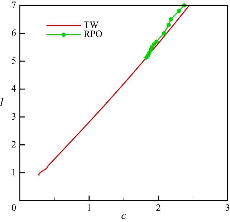
6. Summary and conclusions
In the present paper, we have investigated the dynamics of a coating flow driven by gravity over a fibre rotating about its axis. The evolution equation for the surface is derived in the framework of the long-wave theory with an assumption that the characteristic radius of fluid ring is much smaller than the capillary length scale. The parameters  $a$,
$a$,  $\epsilon$ and $\Omega _N$ are involved in the evolution equation.
A linear stability analysis is performed to examine the influence of rotation on the stability of axisymmetric disturbances. The result of linear stability shows that the rotation is destabilizing without changing the phase speed of the disturbance. The growth rate and the wavenumber of the most unstable mode,  $\lambda _m$ and $k_m$, are proportion to $(1+\Omega _N)^{2}$ and $(1+\Omega _N)^{1/2}$, respectively. We also performed a spatio-temporal stability analysis to examine the effect of rotation on the characteristics of the absolute and convective instabilities. The results showed that the increase of $\Omega _N$ promotes the absolute instability. The result of the spatio-temporal stability analysis was validated by comparison with numerical simulations on the nonlinear evolution of the long-wave model equation. The results of numerical simulations indicate that with the increase of $\Omega _N$ the convectively unstable flow can become absolutely unstable. This result is in excellent agreement with the linear spatio-temporal stability analysis.
The travelling-wave solutions were solved using the Newton method with branch continuation. The effect of rotation on the structure and speed of these solutions was analysed. When the rotation is slow,  $\Omega _N<0.5$, we observed that the travelling-wave speed is promoted by the axial rotation because the height of the droplet becomes larger. However, the travelling-wave speed starts to decrease as the rotation speed increases further because of the strong reversal flow in the wave hump, which retards the motion of droplets.
Linear stability analysis of the travelling-wave solutions was investigated, which showed that the travelling-wave solutions could lose their stabilities to an oscillatory mode when the wavelength exceeds the critical value. With the increase of  $\Omega _N$, the travelling-wave solutions become more stable. When the travelling wave is unstable, the disturbance evolves into a near recurrent solution, which was identified as an RPO. We demonstrated that there exists series of RPOs, which are born from the travelling-wave solutions through Hopf bifurcations. Numerical solutions also demonstrate that axial rotation accelerates the mean wave speed of the RPOs and reduce their periods, indicating that axial rotation can promote the droplet coalescence and breakup process in the system.
Acknowledgments
R.L. is supported by The National Natural Science Foundation of China (grant no. 51766002) and The Guangxi Natural Science Foundation (no. 2018GXNSFAA281331). Z.D. is supported by an EPSRC grant optimisation in fluid mechanics EP/P000959/1 and Heilongjiang Touyan Innovation Team Program.
Declaration of interests
The authors report no conflict of interest.
Appendix A. Direct simulations on the evolution of coating flow
In § 2.2, the results of linear stability analysis showed that both the axisymmetric mode and the non-axisymmetric mode with  $m=1$, $k=0$ can be the most unstable mode. In the appendix, we will perform direct simulations on the nonlinear evolutions on these two cases. For the axisymmetric case, the results of the Navier–Stokes equations are used to validate the long wave model. For the non-axisymmetric case with $m=1$, $k=0$, no asymptotic model has been derived for thick films. The nonlinear evolution has to be examined based on the direct simulations.
A.1. Axisymmetric case
For axisymmetric problem, i.e.  $\partial _\theta =0$ for all variables, we introduce the coordinate transformation
 \begin{equation} t=\tilde{t},\ z=\tilde{z},\ r=h(\tilde{z}, \tilde{t})\tilde{r}+a, \end{equation}
where the thickness of the film  $h(\tilde {z},\tilde {t})=S(\tilde {z},\tilde {t})-a$. This set of mappings transforms an arbitrarily shaped flow region to a rectangular region. The first-order derivatives read
 \begin{equation} \partial_r=\frac{1}{h}\partial_{\tilde{r}}, \partial_z=\partial_{\tilde{z}}-\frac{\partial_{\tilde{z}}h}{h}\tilde{r}\partial_{\tilde{r}}, \partial_t=\partial_{\tilde{t}}-\tilde{r}\frac{\partial_{\tilde{t}}h}{h}\partial_{\tilde{r}}, \end{equation}
and the second-order derivatives read
 \begin{gather} \partial_{rr}=\frac{1}{h^{2}}\partial_{\tilde{r}\tilde{r}},\nonumber\\ \partial_{zz}= \partial_{\tilde{z}\tilde{z}}+ \left[2\left(\frac{\partial_{\tilde{z}}h}{h}\right)^{2}-\frac{\partial_{\tilde{z}\tilde{z}}h}{h}\right]\tilde{r}\partial_{\tilde{r}} -2\frac{\partial_{\tilde{z}}h}{h}\tilde{r}\partial_{\tilde{r}\tilde{z}} +\left(\frac{\partial_{\tilde{z}}h}{h}\right)^{2}\tilde{r}^{2}\partial_{\tilde{r}\tilde{r}}. \end{gather}
Inserting (A 2) and (A 3) into the Navier–Stokes equations yields
 \begin{gather} \left(\frac{1}{h}\partial_{\tilde{r}} +\frac{1}{r}\right)u+\left(\partial_{\tilde{z}}-\frac{\partial_{\tilde{z}}h}{h}\tilde{r}\partial_{\tilde{r}}\right) w=0, \end{gather}
 \begin{gather} \epsilon^{2} Re\left\{\left(\partial_{\tilde{t}}-\tilde{r}\frac{\partial_{\tilde{t}}h}{h}\partial_{\tilde{r}}\right)u+F_u\right\} =-\epsilon^{-2}\frac{1}{h}\partial_{\tilde{r}}p+\epsilon^{-2}\Omega_N (h \tilde{r}+a)+\left({\rm \Delta}-\frac{1}{r^{2}}\right)u, \end{gather}
 \begin{gather} \epsilon^{2} Re\left\{\left(\partial_{\tilde{t}}-\tilde{r}\frac{\partial_{\tilde{t}}h}{h}\partial_{\tilde{r}}\right)w+F_w\right\}=1-\left(\partial_{\tilde{z}}-\frac{\partial_{\tilde{z}}h}{h}\tilde{r}\partial_{\tilde{r}}\right)p+{\rm \Delta} w, \end{gather}
in which
 \begin{align} {\rm \Delta}=\frac{1}{h^{2}}\partial_{\tilde{r}\tilde{r}}+\frac{1}{rh}\partial_{\tilde{r}}+\epsilon^{2}\left\{ \partial_{\tilde{z}\tilde{z}}+ \left[2\left(\frac{\partial_{\tilde{z}}h}{h}\right)^{2}-\frac{\partial_{\tilde{z}\tilde{z}}h}{h}\right]\tilde{r}\partial_{\tilde{r}} -2\frac{\partial_{\tilde{z}}h}{h}\tilde{r}\partial_{\tilde{r}\tilde{z}} +\left(\frac{\partial_{\tilde{z}}h}{h}\right)^{2}\tilde{r}^{2}\partial_{\tilde{r}\tilde{r}}\right\}, \end{align}
and
 \begin{equation} F_u=u\frac{1}{h}\partial_{\tilde{r}}u+w\left(\partial_{\tilde{z}}-\frac{\partial_{\tilde{z}}h}{h}\tilde{r}\partial_{\tilde{r}}\right)u, \end{equation}
 \begin{equation} F_w=u\frac{1}{h}\partial_{\tilde{r}}w+w\left(\partial_{\tilde{z}}-\frac{\partial_{\tilde{z}}h}{h}\tilde{r}\partial_{\tilde{r}}\right)w. \end{equation}
The boundary conditions at the fibre wall are
 \begin{equation} u=w=0, \end{equation}
and at the surface are
 \begin{gather} -\frac{2\epsilon^{2}}{1+\epsilon^{2} \left(\partial_{\tilde{z}}S\right)^{2}}\left\{\left[1+\epsilon^{2}(\partial_{\tilde{z}}S)^{2}\right]\frac{u}r+\partial_{\tilde{z}}w+\epsilon^{2}\partial_{\tilde{z}}S\partial_{\tilde{z}}u\right\}\nonumber\\ \qquad =p-\frac{1}{S\left[1+\epsilon^{2} \left(\partial_{\tilde{z}}S\right)^{2}\right]^{1/2}}+\frac{\epsilon^{2}\partial_{\tilde{z}\tilde{z}}S}{\left[1+\epsilon^{2} \left(\partial_{\tilde{z}}S\right)^{2}\right]^{3/2}}, \end{gather}
 \begin{align} & \frac{\left[1+\epsilon^{2}\left(\partial_{\tilde{z}}S\right)^{2}\right]^{2}}{h}\partial_{\tilde{r}}w\nonumber\\ &\quad =\epsilon^{2}\left[3+\epsilon^{2}\left(\partial_{\tilde{z}}S\right)^{2}\right]\partial_{\tilde{z}}S\partial_{\tilde{z}}w -\epsilon^{2}\left(1-\epsilon^{2}\partial_{\tilde{z}} S^{2}\right)\partial_{\tilde{z}}u+\left[1+\epsilon^{2}\left(\partial_{\tilde{z}} S\right)^{2}\right]\epsilon^{2} \partial_{\tilde{z}} S\frac{u}{r}, \end{align}
 \begin{align} \partial_{\tilde{t}} S^{2}+2\partial_{\tilde{z}}\left( \int_a^{S} wr \,\textrm{d}r\right)=0. \end{align}
 The rectangular domain is discretized by the Fourier–Chebyshev method, grid  $[\tilde {z}_1, \tilde {z}_2,\ldots , \tilde {z}_M]\times [\tilde {r}_1, \tilde {r}_2,\ldots , \tilde {r}_N]$ with $M$ and $N$ mesh points in $\tilde {z}$ and $\tilde {r}$ directions, respectively. The temporal evolution of the problem is obtained by two steps:
 \begin{gather}\left.\begin{aligned} h(\tilde{z},\tilde{t})\rightarrow h(\tilde{z},\tilde{t}+\delta \tilde{t}), \quad\quad \\ (u,w)(\tilde{z},\tilde{t})\rightarrow (u,w)(\tilde{z},\tilde{t}+\delta \tilde{t}). \end{aligned}\right\}\end{gather}
For more details of the procedure of the time stepping, we refer the readers to the work by Richter & Bestehorn (Reference Richter and Bestehorn2019) in which an algorithm based on a nonlinear coordinate transformation is used for direct numerical simulations of liquid films under horizontal and vertical external vibrations.
In order to validate our long-wave model, we have compared the travelling-wave solutions of the long-wave model with that of the Navier–Stokes equations for several sets of parameters. The results of the Navier–Stokes equations are the saturated states of the most unstable modes after a long-time evolution. In figure 17, we present the results of these two models for  $\Omega _N=0$ and 0.5. As shown in figure 17(a,b), the profiles of the interface of the long-wave mode are similar to those of the Navier–Stokes equations. In figure 18, we compare the maximum of the position of the interface, $S_{\textit{max}}$, of the long-wave model and Navier–Stokes for various $\Omega _N$. As shown in this figure, the results of the long-wave model are in good agreement with those of the Navier–Stokes equations. This means that the long-wave model is valid for the parameters in the present study.
The profiles of the interface of the travelling-wave solution of the full Navier–Stokes equations (NS) and the long-wave model (LW). ( $a) \ \Omega _N=0.0$; ( $b) \ \Omega _N=0.5$. Other parameters are $\epsilon = 0.2$, $a=0.25$ and $l=2$.
The comparison between the travelling-wave solution of the full Navier–Stokes equations (NS) and the long-wave model (LW) for various  $\Omega _N$. Other parameters are $\epsilon = 0.2$, $a=0.25$ and $l=2$.
A.2. Non-axisymmetric case of  $k=0$
$k=0$

For the non-axisymmetric case of  $k=0$, the flow is streamwise uniform, i.e. $\partial _z=0$. The controlling equations are expressed as
 \begin{gather} \partial_r u+\frac{u}{r}+\frac{1}{r}\partial_\theta v=0, \end{gather}
 \begin{gather} \epsilon^{4} Re\left(\partial_t u+{u}\partial_r u+\frac{v}{r}\partial_\theta u-\frac{v^{2}}{r}\right)=-\partial_r p+\Omega_N r+ \epsilon^{2}\left[\partial_{rr}u+\frac{\partial_r u}{r}+\frac{1}{r^{2}}\partial_{\theta\theta}u-\frac{u}{r^{2}}\right], \end{gather}
 \begin{gather} \epsilon^{4} Re\left(\partial_t v+{u}\partial_r v+\frac{v}{r}\partial_\theta v+\frac{uv}{r}\right)=-\frac{1}{r}\partial_\theta p+ \epsilon^{2}\left[\partial_{rr}v+\frac{\partial_r v}{r}+\frac{1}{r^{2}}\partial_{\theta\theta}v-\frac{v}{r^{2}}\right]. \end{gather}
At the fibre wall ( $r=a$), the boundary conditions are
 \begin{equation} u=v=0. \end{equation}
At the free surface, the boundary conditions are
 \begin{gather} \left[1-\left(\frac{\partial_\theta S}{r}\right)^{2}\right]\left\{r\partial_r\left(\frac{v}{r}\right)+\frac{\partial_\theta u}{r}\right\}+2\frac{\partial_\theta S}{r}\left(\partial_r u-\frac{\partial_\theta v}{r}-\frac{u}{r}\right)=0, \end{gather}
 \begin{gather} -p+2\epsilon^{2} N^{-2}\left\{\partial_ru-\frac{\partial_\theta S}{r}\left[r\partial_r\left(\frac{v}{r}\right)+\frac{\partial_\theta u}{r}\right]+ \left(\frac{\partial_\theta S}{r}\right)^{2}\left(\frac{\partial_\theta v}{r}+\frac{u}{r}\right)\right\}=2H, \end{gather}
 \begin{gather} S_t+\frac{1}{S}\partial_\theta \int_a^{S} v \,\textrm{d}r=0. \end{gather}
in which the principal curvature
 \begin{equation} 2H=-\frac{1}{N}\left\{\frac{1}{S}+\frac{\left(\partial_\theta S\right)^{2}}{S^{3}}-\frac{\partial_{\theta\theta}S}{S^{2}}\right\}-\frac{1}{N^{2}}\frac{\partial_\theta N \partial_\theta S}{S^{2}}, \end{equation}
where
 \begin{equation} N=\sqrt{1+r^{-2}(\partial_\theta S)^{2}}. \end{equation}
We introduced the coordinate transformation
 \begin{equation} t=\tilde{t},\ \theta=\tilde{\theta},\ r=h(\tilde{\theta},\ \tilde{t})\tilde{r}+a, \end{equation}
where the thickness of the film  $h=S(\theta ,t)-a$. The first-order derivatives
 \begin{equation} \partial_r=\frac{1}{h}\partial_{\tilde{r}},\ \partial_\theta=\partial_{\tilde{\theta}}-\frac{\partial_{\tilde{\theta}}h}{h}\tilde{r}\partial_{\tilde{r}},\ \partial_t=\partial_{\tilde{t}}-\tilde{r}\frac{\partial_{\tilde{t}}h}{h}\partial_{\tilde{r}}, \end{equation}
and the second-order derivatives
 \begin{align} &\partial_{rr}=\frac{1}{h^{2}}\partial_{\tilde{r}\tilde{r}},\nonumber\\ &\partial_{\theta\theta}= \partial_{\tilde{\theta}\tilde{\theta}}+ \left[2\left(\frac{\partial_{\tilde{\theta}}h}{h}\right)^{2}-\frac{\partial_{\tilde{\theta}\tilde{\theta}}h}{h}\right]\tilde{r}\partial_{\tilde{r}} -2\frac{\partial_{\tilde{\theta}}h}{h}\tilde{r}\partial_{\tilde{r}\tilde{\theta}} +\left(\frac{\partial_{\tilde{\theta}}h}{h}\right)^{2}\tilde{r}^{2}\partial_{\tilde{r}\tilde{r}}. \end{align}
The numerical method for solving the problem is similar to the axisymmetric case.
In the numerical simulations, the initial state is given by
 \begin{equation} S(\theta,0)=1+\delta\cos(\theta), \end{equation}
in which  $\delta$ is a small number. At the initial time, the maximum and the minimum of $S$ locates at $\theta =0$ and $\theta ={\rm \pi}$, respectively. Because of the destabilizing effect of rotation, the film thickness increases with time near the region of $\theta =0$ and the decreases gradually on the opposite side. After a long-time evolution, the film thickness at $\theta ={\rm \pi}$ approaches zero. This process corresponds to the fluid detachment from the substrate. As the minimum thickness approaches zero, the stiffness of the numerical procedure increases dramatically. In our simulations, we terminate the process of time stepping when the minimum thickness is close to 0.01. In figure 19, we present the profile of the free surface of the evolution of the non-axisymmetric mode with $m=1$ and $k=0$ when the film is close to the detachment. As shown in figure 19(a) for $a=0.8$, the profile of the free surface is close to a circle. However, as shown in figure 19(b) for $a=0.3$, the profile evolves into a flat lobe due to the destabilizing body force.
The profile of free surface of the evolution of the non-axisymmetric mode with  $m=1$ and $k=0$. ( $a$) For $a=0.8$; ( $b$) for $a=0.3$. The parameters $\epsilon =0.3$ and $\Omega _N=0.489$ corresponding to the frequency of rotation $f=20$.
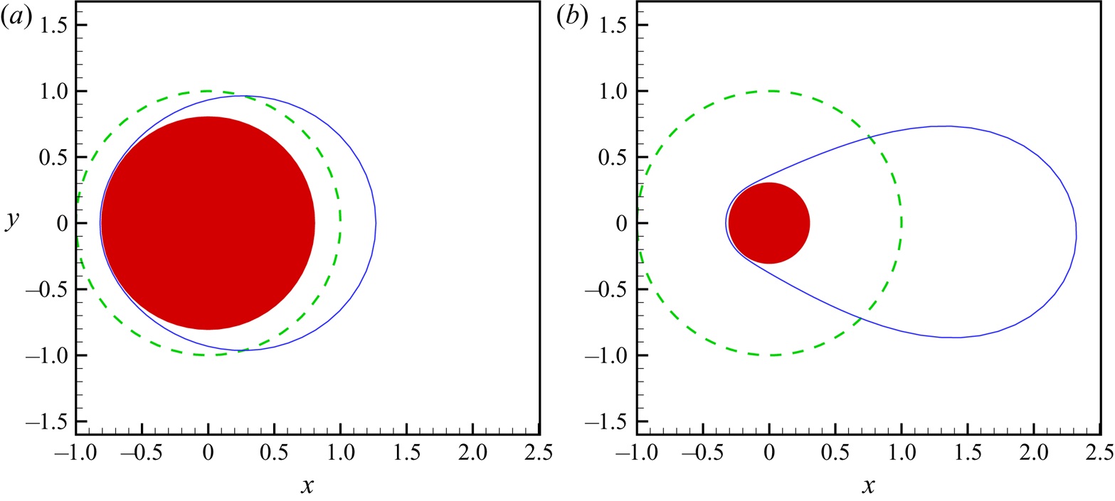
The simulations on the disturbance with  $m=1$ and $k=0$ showed the process of detachment from the substrate. However, these streamwise uniform surface is unstable due to the Rayleigh–Plateau mechanism. We can expect that in the process of detachment, there exists the formation of non-axisymmetric beads. The dynamics of this complex process needs further investigation on the stability analysis of the full linearized Navier–Stokes equations.
Appendix B. Thin film model for 3-D evolutions
We introduce the dimensionless variables as follows:
 \begin{equation} (r,z)=a (r^{\ast}, z^{\ast}),\ y=H y^{\ast},\ t=aV^{-1}t^{\ast},\ (u,v,w)=V(\varepsilon u^{\ast},\ v^{\ast},w^{\ast}),\ p=\rho g a p^{\ast}, \end{equation}
where the star,  $^{\ast }$, denotes dimensionless variables. A new variable is introduced, $y=r-a$, in the terms related to $\partial _r$. The aspect ratio $\varepsilon =H/a$, the velocity scale $V\equiv \rho g H^{2}/\mu$ in which $H=R-a$. We consider the thin film problem in which $\varepsilon \ll 1$.
For simplicity, we dropped  $^{\ast }$ for all dimensionless variables. Neglecting the contribution of inertial terms and the higher terms of $\varepsilon$ The dimensionless nonlinear evolution equation is expressed as
 \begin{equation} S\partial_t S+\partial_\theta Q_\theta+\partial_z Q_z=0, \end{equation}
in which
 \begin{gather} Q_\theta=\varepsilon^{-2}\partial_\theta p\left\{ \frac{1}{\ln S-1}+\frac{1}{2}(S^{2}+1)\right\}, \end{gather}
 \begin{gather} Q_z=\varepsilon^{-2}(\partial_z p-1)\left\{\frac{(S^{2}-1)(3S^{2}-1)}{16}-\frac{1}{4}S^{4}\ln S\right\}, \end{gather}
 \begin{gather} p=\frac{1}{2}\varepsilon^{-1}\Omega_N'(r^{2}-S^{2})+Ca^{-1}\left[\frac{1}{S}- \frac{\partial_{\theta\theta} S}{S^{2}}-\partial_{zz}S\right]. \end{gather}
The parameter  $\Omega _N'=a\Omega ^{2}/g$ and $Ca=\rho g a^{2}/\sigma$. Note that when discussing the results, we used $\Omega _N$ instead of $\Omega _N'$.
The linear stability analysis showed that both axisymmetric and non-axisymmetric disturbance can be the unstable mode. For the nonlinear dynamics in fluid mechanics, many previous studies showed that the transition has non-unique routes, which depend on the initial conditions. In this appendix, we will show that there exists different routes of evolutions for various rotation parameters.
Firstly, we study the case of a small rotation number. We choose the parameters  $\Omega _N=0.122$ and $\varepsilon = 0.3$ as in figure 2. For a non-axisymmetric initial condition (there is no streamwise component), $h=1+\delta \sin (\theta )$ or $h=1+\delta \sin (\theta +kz)$, the flow is unstable and a non-axisymmetric and a streamwise uniform state can develop. But if there is a streamwise component (we set $h=1+\delta \sin (\theta )+\delta \sin (kz)$), we observe that the final state is axisymmetric which indicates that the non-axisymmetric mode is suppressed by the axisymmetric mode (see figure 20). This study indicates that the axisymmetric state will be observed in experiments when the rotation is slow, because the axisymmetric mode is the most unstable and grows fastest.
The profile of the surface at the saturated state for the case at  $\Omega _N=0.122$, $\epsilon = 0.3$. The dimensional parameters are $a=0.8 \ \textrm {mm}$ and the thickness is $H=0.2 \ \textrm {mm}$.
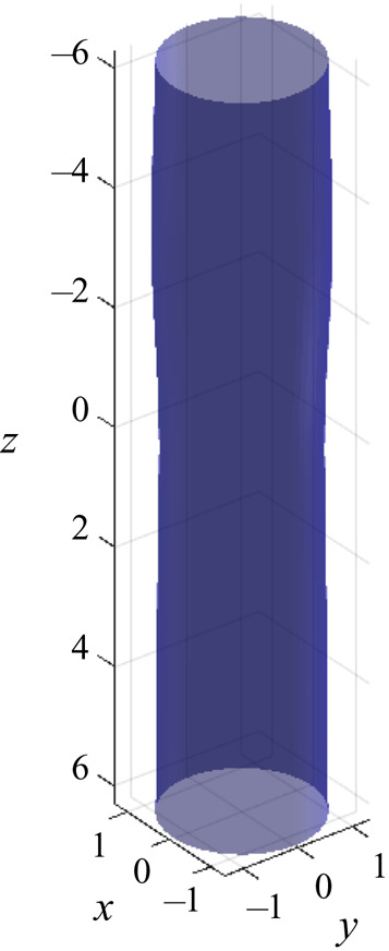
We also studied the case of a large rotation number. We choose  $\Omega _N=0.5$ and $\varepsilon =0.3$ as in figure 2. We tested two different initial conditions, $h=1+\delta \sin (\theta )+\delta \sin (kz))$ and $h=1+\delta \sin (kz)$. For the axisymmetric initial condition, we observe that the state remains axisymmetric. However, as expected, a 3-D state develops when the system is perturbed by the non-axisymmetric initial condition (see figure 21). However, if we rotate the cylinder after the formation of axisymmetric beads (or perturb the saturated axisymmetric state by non-axisymmetric disturbances), we did observe that the system reverts back to the axisymmetric state in the parametric space considered in the present study (see figure 22). This demonstrates that we may observe an axisymmetric film in experiments if we gradually increase the rotation speed or rotate the cylinder after the formation of axisymmetric beads.
The profile of the surface at the saturated state for the case at  $\Omega _N=0.5$, $\epsilon =0.3$. The dimensional parameters are $a=0.8 \ \textrm {mm}$ and the thickness is $H=0.2 \ \textrm {mm}$.
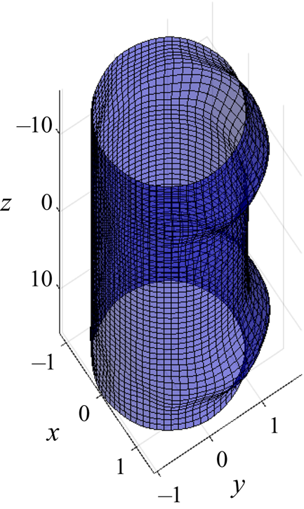
The profile of the surface at the saturated state for the case at  $\Omega _N=0.5$, $\epsilon =0.3$. The dimensional parameters are $a=0.8 \ \textrm {mm}$ and the thickness is $H=0.2 \ \textrm {mm}$. Here we perturbed the saturated axisymmetric state by a non-axisymmetric disturbance.
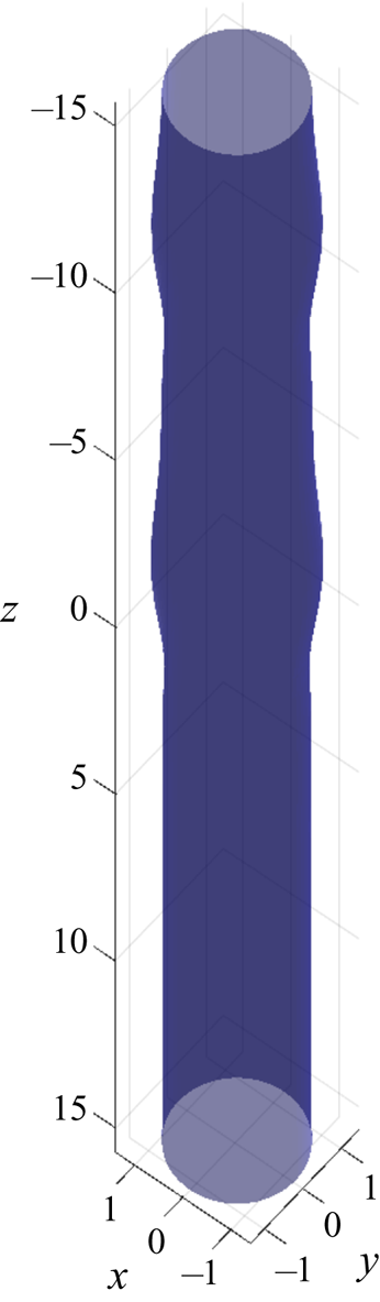


 Open access