


1. Introduction
Upon impacting a solid surface, the momentum of a falling droplet is counterbalanced by inertia, viscous dissipation and surface tension, which governs fluid retraction (Pasandideh-Fard et al. Reference Pasandideh-Fard, Qiao, Chandra and Mostaghimi1996; Josserand & Thoroddsen Reference Josserand and Thoroddsen2016). The resulting deformation exhibits complex dynamics, including oscillations, sheet formation during spreading and jetting upon retraction (Yarin & Weiss Reference Yarin and Weiss1995; Zhang et al. Reference Zhang, Sanjay, Shi, Zhao, Lv, Feng and Lohse2022). Similarly rich dynamics is observed when droplets splash on pillars (Villermaux & Bossa Reference Villermaux and Bossa2011; Wang et al. Reference Wang, Dandekar, Bustos, Poulain and Bourouiba2018). Deformations may also occur under the influence of external flows where a wide range of phenomena from droplet vibration (Pilch & Erdman Reference Pilch and Erdman1987; Hsiang & Faeth Reference Hsiang and Faeth1992) to bag breakup (Guildenbecher, López-Rivera & Sojka Reference Guildenbecher, López-Rivera and Sojka2009; Jalaal & Mehravaran Reference Jalaal and Mehravaran2012; Jackiw & Ashgriz Reference Jackiw and Ashgriz2021), sheet stripping (Theofanous Reference Theofanous2011; Jalaal & Mehravaran Reference Jalaal and Mehravaran2014) and catastrophic fragmentation (Guildenbecher et al. Reference Guildenbecher, López-Rivera and Sojka2009; Theofanous Reference Theofanous2011) may occur. The resulting dynamics is often characterised by the Weber number, ${\textit{We}}=\rho D_0 U^2/\sigma$
(with the liquid density
${\textit{We}}=\rho D_0 U^2/\sigma$
(with the liquid density $\rho$
in droplet impact experiments, droplet diameter
$\rho$
in droplet impact experiments, droplet diameter $D_0$
, impact velocity
$D_0$
, impact velocity $U$
and surface tension
$U$
and surface tension $\sigma$
; for wind-driven droplet fragmentation, the relevant air density and velocity are taken instead), and the Ohnesorge number that relates the viscous forces to inertial and surface tension forces. In contrast to previous methods, using a laser impact on a droplet offers a unique opportunity to precisely control the pressure profile on its surface. In wind tunnel experiments, the entire surrounding medium is in motion, which complicates any effort to stabilise or adjust the pressure profile on the droplet surface. Similarly, when employing a fixed pillar to perturb the droplet, the pillar remains in continuous contact with the droplet, and neither the tunnel nor the pillar technique provides instantaneous control. As a result, in all these approaches, the droplet’s response is primarily determined by the impact velocity
$\sigma$
; for wind-driven droplet fragmentation, the relevant air density and velocity are taken instead), and the Ohnesorge number that relates the viscous forces to inertial and surface tension forces. In contrast to previous methods, using a laser impact on a droplet offers a unique opportunity to precisely control the pressure profile on its surface. In wind tunnel experiments, the entire surrounding medium is in motion, which complicates any effort to stabilise or adjust the pressure profile on the droplet surface. Similarly, when employing a fixed pillar to perturb the droplet, the pillar remains in continuous contact with the droplet, and neither the tunnel nor the pillar technique provides instantaneous control. As a result, in all these approaches, the droplet’s response is primarily determined by the impact velocity $U$
.
$U$
.
Nevertheless, the force distribution on the surface is well known to significantly influence droplet deformation behaviour at high We (Gelderblom et al. Reference Gelderblom, Lhuissier, Klein, Bouwhuis, Lohse, Villermaux and Snoeijer2016; Hernandez-Rueda et al. Reference Hernandez-Rueda, Liu, Hemminga, Mostafa, Meijer, Kurilovich, Basko, Gelderblom, Sheil and Versolato2022; França et al. Reference França, Schubert, Versolato and Jalaal2025), as established in the context of laser-driven droplet deformation for nanolithography (Versolato Reference Versolato2019). The interaction between nanosecond-pulsed laser light with micrometre-sized tin droplets is a relevant source of extreme ultraviolet (EUV) light, as used in state-of-the-art industrial nanolithography. The generation of EUV light involves the laser-impact deformation of a tin droplet into a thin sheet that is subsequently laser-heated into an EUV-emitting plasma. Upon ( $\sim 10\,\textrm {mJ}$
) laser-pulse impact, a plasma is generated from the droplet surface and produces a recoil pressure of the order of
$\sim 10\,\textrm {mJ}$
) laser-pulse impact, a plasma is generated from the droplet surface and produces a recoil pressure of the order of $\sim 100$
kbar. In a typical setting, the droplet is accelerated on the laser-pulse length scale,
$\sim 100$
kbar. In a typical setting, the droplet is accelerated on the laser-pulse length scale, $\tau _{\!p}\sim 10\,\textrm {ns}$
, reaching terminal velocities of the order of
$\tau _{\!p}\sim 10\,\textrm {ns}$
, reaching terminal velocities of the order of $U\sim 100\,\rm {m\,s}^{-1}$
while it radially expands. The corresponding large Weber number is in the range
$U\sim 100\,\rm {m\,s}^{-1}$
while it radially expands. The corresponding large Weber number is in the range $\sim 1000{-}10\,000$
; hence, the droplet transforms into a time-varying radially expanding liquid sheet (Kurilovich et al. Reference Kurilovich, Klein, Torretti, Lassise, Hoekstra, Ubachs, Gelderblom and Versolato2016, Reference Kurilovich, Basko, Kim, Torretti, Schupp, Visschers, Scheers, Hoekstra, Ubachs and Versolato2018; Liu et al. Reference Liu, Meijer, Hernandez-Rueda, Kurilovich, Mazzotta, Witte and Versolato2021, Reference Liu, Meijer, Li, Hernandez-Rueda, Gelderblom and Versolato2023), undergoing several hydrodynamical instabilities responsible for its rupture through hole opening (Klein et al. Reference Klein, Kurilovich, Lhuissier, Versolato, Lohse, Villermaux and Gelderblom2020a
) or radial accumulation of the liquid into a fragmenting bounding rim (Wang et al. Reference Wang, Dandekar, Bustos, Poulain and Bourouiba2018; Wang & Bourouiba Reference Wang and Bourouiba2021).
$\sim 1000{-}10\,000$
; hence, the droplet transforms into a time-varying radially expanding liquid sheet (Kurilovich et al. Reference Kurilovich, Klein, Torretti, Lassise, Hoekstra, Ubachs, Gelderblom and Versolato2016, Reference Kurilovich, Basko, Kim, Torretti, Schupp, Visschers, Scheers, Hoekstra, Ubachs and Versolato2018; Liu et al. Reference Liu, Meijer, Hernandez-Rueda, Kurilovich, Mazzotta, Witte and Versolato2021, Reference Liu, Meijer, Li, Hernandez-Rueda, Gelderblom and Versolato2023), undergoing several hydrodynamical instabilities responsible for its rupture through hole opening (Klein et al. Reference Klein, Kurilovich, Lhuissier, Versolato, Lohse, Villermaux and Gelderblom2020a
) or radial accumulation of the liquid into a fragmenting bounding rim (Wang et al. Reference Wang, Dandekar, Bustos, Poulain and Bourouiba2018; Wang & Bourouiba Reference Wang and Bourouiba2021).
Laser-induced droplet deformation has been shown to be well described by the impact propulsion Weber number ${\textit{We}}=\rho D_0 U^2/\sigma$
, based on centre-of-mass propulsion velocity
${\textit{We}}=\rho D_0 U^2/\sigma$
, based on centre-of-mass propulsion velocity $U$
, and deformation Weber number (Klein et al. Reference Klein, Kurilovich, Lhuissier, Versolato, Lohse, Villermaux and Gelderblom2020b
; Liu et al. Reference Liu, Hernandez-Rueda, Gelderblom and Versolato2022)
$U$
, and deformation Weber number (Klein et al. Reference Klein, Kurilovich, Lhuissier, Versolato, Lohse, Villermaux and Gelderblom2020b
; Liu et al. Reference Liu, Hernandez-Rueda, Gelderblom and Versolato2022) ${\textit{We}}_{{d}}=\rho D_0\dot {R}_0^2/\sigma$
, based on radial expansion rate
${\textit{We}}_{{d}}=\rho D_0\dot {R}_0^2/\sigma$
, based on radial expansion rate $\dot {R}_0$
; these two orthogonal velocities, as shown in figure 1, are correlated and both increase with increasing laser-pulse energy (Gelderblom et al. Reference Gelderblom, Lhuissier, Klein, Bouwhuis, Lohse, Villermaux and Snoeijer2016; Hernandez-Rueda et al. Reference Hernandez-Rueda, Liu, Hemminga, Mostafa, Meijer, Kurilovich, Basko, Gelderblom, Sheil and Versolato2022). Additionally, to properly account for the droplet curvature after laser impact, França et al. (Reference França, Schubert, Versolato and Jalaal2025) described the resulting pressure profile in terms of a raised cosine function projected on the surface
$\dot {R}_0$
; these two orthogonal velocities, as shown in figure 1, are correlated and both increase with increasing laser-pulse energy (Gelderblom et al. Reference Gelderblom, Lhuissier, Klein, Bouwhuis, Lohse, Villermaux and Snoeijer2016; Hernandez-Rueda et al. Reference Hernandez-Rueda, Liu, Hemminga, Mostafa, Meijer, Kurilovich, Basko, Gelderblom, Sheil and Versolato2022). Additionally, to properly account for the droplet curvature after laser impact, França et al. (Reference França, Schubert, Versolato and Jalaal2025) described the resulting pressure profile in terms of a raised cosine function projected on the surface $\sim (1+\cos (\theta \pi /{W} ) )H({W}-\theta )$
(figure 1
a,b), where W is a dimensionless pressure width and
$\sim (1+\cos (\theta \pi /{W} ) )H({W}-\theta )$
(figure 1
a,b), where W is a dimensionless pressure width and $H({W}-\theta )$
is the Heaviside step function. This parameter W can be interpreted as a measure of the spatial, angular extent of the pressure imprinted on the droplet by the laser plasma, as illustrated in figure 1(a): increasing
$H({W}-\theta )$
is the Heaviside step function. This parameter W can be interpreted as a measure of the spatial, angular extent of the pressure imprinted on the droplet by the laser plasma, as illustrated in figure 1(a): increasing ${W}$
leads to a broader pressure field on the droplet, which manifests as a broader early-time deformation characterised by a larger opening angle
${W}$
leads to a broader pressure field on the droplet, which manifests as a broader early-time deformation characterised by a larger opening angle $\theta _{\textit{open}}$
(figure 1
a,c–e). Further details are discussed in § 3.1. This pressure profile accurately describes the sheet morphology over a range of pressure widths
$\theta _{\textit{open}}$
(figure 1
a,c–e). Further details are discussed in § 3.1. This pressure profile accurately describes the sheet morphology over a range of pressure widths $1\lt {W}\lt 2.5$
as shown by França et al. (Reference França, Schubert, Versolato and Jalaal2025). We illustrate the impact of the propulsion We with the pressure width W on the pressure field separately in figure 1(b) (see § 2.2). The three parameters (We, We
$1\lt {W}\lt 2.5$
as shown by França et al. (Reference França, Schubert, Versolato and Jalaal2025). We illustrate the impact of the propulsion We with the pressure width W on the pressure field separately in figure 1(b) (see § 2.2). The three parameters (We, We $_{{d}}$
, W) are correlated and the function We
$_{{d}}$
, W) are correlated and the function We $_{{d}}$
=
$_{{d}}$
= $f$
(We, W) is set by an initial, instantaneous pressure profile with essentially two free parameters being its amplitude and width (França et al. Reference França, Schubert, Versolato and Jalaal2025) (see § 3.1). For a more comprehensive study of the separate influence of laser spot size, droplet diameter and laser-pulse energy on the plasma-induced velocities (
$f$
(We, W) is set by an initial, instantaneous pressure profile with essentially two free parameters being its amplitude and width (França et al. Reference França, Schubert, Versolato and Jalaal2025) (see § 3.1). For a more comprehensive study of the separate influence of laser spot size, droplet diameter and laser-pulse energy on the plasma-induced velocities ( $U,\dot {R}_0$
) we refer the reader to Hernandez-Rueda et al. (Reference Hernandez-Rueda, Liu, Hemminga, Mostafa, Meijer, Kurilovich, Basko, Gelderblom, Sheil and Versolato2022).
$U,\dot {R}_0$
) we refer the reader to Hernandez-Rueda et al. (Reference Hernandez-Rueda, Liu, Hemminga, Mostafa, Meijer, Kurilovich, Basko, Gelderblom, Sheil and Versolato2022).
(a) Conceptual side-view representation of laser–droplet interaction. The laser beam is represented as a red area. After laser impact, the droplet is propelled axially at $U$
while radially expanding at
$U$
while radially expanding at $\dot {R}_0$
initially. The force profile resulting from laser–plasma interaction, described as a dimensionless parameter
$\dot {R}_0$
initially. The force profile resulting from laser–plasma interaction, described as a dimensionless parameter ${W}$
, is proportional to early-time deformation (see main text). The angular distribution of the resulting pressure is depicted in (b) where curves show different values of pressure distribution on the droplet’s surface. The black and orange curves with the same value of
${W}$
, is proportional to early-time deformation (see main text). The angular distribution of the resulting pressure is depicted in (b) where curves show different values of pressure distribution on the droplet’s surface. The black and orange curves with the same value of ${W}$
depict different values of
${W}$
depict different values of ${\textit{We}}$
(higher and lower, respectively). The dashed line illustrates the width of the pressure distribution for
${\textit{We}}$
(higher and lower, respectively). The dashed line illustrates the width of the pressure distribution for ${W}=1$
. (c–e) Experimental examples of the hydrodynamic response after laser interaction with a droplet with diameter
${W}=1$
. (c–e) Experimental examples of the hydrodynamic response after laser interaction with a droplet with diameter $D_0=50\,\unicode{x03BC} \textrm {m}$
. Each row contains frames at different fractions of capillary times,
$D_0=50\,\unicode{x03BC} \textrm {m}$
. Each row contains frames at different fractions of capillary times, $\tau _{{c}} = 16.4\,\unicode{x03BC} \textrm {s}$
. (c) Droplet oscillation for
$\tau _{{c}} = 16.4\,\unicode{x03BC} \textrm {s}$
. (c) Droplet oscillation for ${\textit{We}}=0.2$
and
${\textit{We}}=0.2$
and ${W}=1.0$
. (d) Droplet breakup after retraction for
${W}=1.0$
. (d) Droplet breakup after retraction for ${\textit{We}}=3.4$
and
${\textit{We}}=3.4$
and ${W}=1.4$
. (e) Sheet expansion for
${W}=1.4$
. (e) Sheet expansion for ${\textit{We}}=154$
and
${\textit{We}}=154$
and ${W}=2$
. The grey scale bar in the first frame in (c) corresponds to
${W}=2$
. The grey scale bar in the first frame in (c) corresponds to $D_0=50\,\unicode{x03BC} \mathrm{m}$
.
$D_0=50\,\unicode{x03BC} \mathrm{m}$
.

Thus, unlike droplet impact on solid surfaces, falling drop or wind tunnel interactions, laser–droplet interaction offers a path to studying how the spatial distribution of the force, along with its overall magnitude, influences droplet dynamics. However, motivated by direct nanolithography applications, prior studies have focused on high Weber numbers that lead to sheet formation.
In this work, we investigate droplet deformation following laser-pulse impact at low Weber numbers ( ${\textit{We}}\sim 0.1{-}100$
) combining experiments with numerical simulations. Decreasing markedly the pulse energy (
${\textit{We}}\sim 0.1{-}100$
) combining experiments with numerical simulations. Decreasing markedly the pulse energy ( $\sim 0.1{-}1\,\textrm {mJ}$
) in the experiment, we mainly focus on the dynamics of the regimes before sheet formation. In figure 1(c–e) we illustrate representative cases of droplet deformation over fractions of the capillary time
$\sim 0.1{-}1\,\textrm {mJ}$
) in the experiment, we mainly focus on the dynamics of the regimes before sheet formation. In figure 1(c–e) we illustrate representative cases of droplet deformation over fractions of the capillary time $\tau _{{c}}=\sqrt {\rho D_0^3/6\sigma }$
, with
$\tau _{{c}}=\sqrt {\rho D_0^3/6\sigma }$
, with $\rho$
and
$\rho$
and $\sigma$
being liquid density and surface tension, respectively. At lower We, an oscillatory motion is observed, as shown in figure 1(c), reminiscent of previous work on oscillating free droplets (see e.g. Becker, Hiller & Kowalewski Reference Becker, Hiller and Kowalewski1991; Hsiang & Faeth Reference Hsiang and Faeth1992; Bostwick & Steen Reference Bostwick and Steen2009; Rimbert et al. Reference Rimbert, Escobar, Meignen, Hadj-Achour and Gradeck2020; Parik, Truscott & Dutta Reference Parik, Truscott and Dutta2024). The symmetry of this oscillation is unavoidably broken given the laser impact geometry. For slightly higher pulse energies the droplet breaks up, as shown in figure 1(d). Finally, at even higher pulse energies, the radial inertia leads to sheet formation, as shown in figure 1(e). For reference, we provide estimates of the corresponding (We, W) values for each case in figure 1, with W obtained using a scaling relation that also involves input from our simulations (see below). The two parameters are strongly correlated in the experiment, with increased pulse energy leading to both increased We and W values. The goal of this study is to characterise the individual influence of these two key parameters on the deformation process for low We. Our experiments traverse a phase space comprising (i) droplet oscillation, (ii) breakup and (iii) sheet formation. Numerical simulations complement the experiments and allow for independently varying We and W.
$\sigma$
being liquid density and surface tension, respectively. At lower We, an oscillatory motion is observed, as shown in figure 1(c), reminiscent of previous work on oscillating free droplets (see e.g. Becker, Hiller & Kowalewski Reference Becker, Hiller and Kowalewski1991; Hsiang & Faeth Reference Hsiang and Faeth1992; Bostwick & Steen Reference Bostwick and Steen2009; Rimbert et al. Reference Rimbert, Escobar, Meignen, Hadj-Achour and Gradeck2020; Parik, Truscott & Dutta Reference Parik, Truscott and Dutta2024). The symmetry of this oscillation is unavoidably broken given the laser impact geometry. For slightly higher pulse energies the droplet breaks up, as shown in figure 1(d). Finally, at even higher pulse energies, the radial inertia leads to sheet formation, as shown in figure 1(e). For reference, we provide estimates of the corresponding (We, W) values for each case in figure 1, with W obtained using a scaling relation that also involves input from our simulations (see below). The two parameters are strongly correlated in the experiment, with increased pulse energy leading to both increased We and W values. The goal of this study is to characterise the individual influence of these two key parameters on the deformation process for low We. Our experiments traverse a phase space comprising (i) droplet oscillation, (ii) breakup and (iii) sheet formation. Numerical simulations complement the experiments and allow for independently varying We and W.
The rest of this article is organised as follows. In § 2.1 we provide a brief explanation of our experimental set-up. § 3 is devoted to the presentation and discussion of the results. The numerical simulations are explained in § 2.2. Next, in § 3.1 we perform an analysis of the pressure profile on the droplet, where we explain how to correlate the droplet inertial deformation with the corresponding pressure projection on the surface. The oscillatory motion of the droplet is discussed in § 3.2. In § 3.3, we illustrate the breakup mechanism and how a further increase in the energy of the laser pulse leads to the familiar scenario where the tin droplet deforms into a radially expanding sheet. To summarise, in § 3.5 we present a phase diagram, combining experiments and simulations, based on the systematic variation of both ${\textit{We}}$
and pressure width
${\textit{We}}$
and pressure width ${W}$
and discuss the boundaries for the different phases.
${W}$
and discuss the boundaries for the different phases.
2. Methods
2.1. Experimental method
We refer the reader to Kurilovich et al. (Reference Kurilovich, Basko, Kim, Torretti, Schupp, Visschers, Scheers, Hoekstra, Ubachs and Versolato2018) and Meijer et al. (Reference Meijer, Kurilovich, Eikema, Versolato and Witte2022b
) for a detailed description of the experimental set-up. Briefly, we use a micro-sized tin liquid jet produced from a pressurised tank placed on the top of a spherical vacuum chamber kept at a base pressure of $10^{-6}$
mbar. The jet is fragmented into a train of equally spaced droplets, depending on the frequency of the voltage pulses applied to the nozzle (Kurilovich et al. Reference Kurilovich, Basko, Kim, Torretti, Schupp, Visschers, Scheers, Hoekstra, Ubachs and Versolato2018). In the current experiments, we produce two different droplet sizes, with diameters
$10^{-6}$
mbar. The jet is fragmented into a train of equally spaced droplets, depending on the frequency of the voltage pulses applied to the nozzle (Kurilovich et al. Reference Kurilovich, Basko, Kim, Torretti, Schupp, Visschers, Scheers, Hoekstra, Ubachs and Versolato2018). In the current experiments, we produce two different droplet sizes, with diameters $D_0=50, 70\,\unicode{x03BC} \textrm {m}$
, with density
$D_0=50, 70\,\unicode{x03BC} \textrm {m}$
, with density $\rho =7000\,\textrm {kg}\,\textrm {m}^{-3}$
, surface tension
$\rho =7000\,\textrm {kg}\,\textrm {m}^{-3}$
, surface tension $\sigma =0.544\,\textrm {N}\,\textrm {m}^{-1}$
and dynamic viscosity
$\sigma =0.544\,\textrm {N}\,\textrm {m}^{-1}$
and dynamic viscosity $\mu =1.8\times 10^{-3}\,\textrm {Pa}\,\textrm {s}$
. The droplet interacts with a circularly polarised
$\mu =1.8\times 10^{-3}\,\textrm {Pa}\,\textrm {s}$
. The droplet interacts with a circularly polarised $1064\,\textrm {nm}$
Nd:YAG laser pulse, with a Gaussian temporal profile of
$1064\,\textrm {nm}$
Nd:YAG laser pulse, with a Gaussian temporal profile of $6\,\textrm {ns}$
and peak energies in the range
$6\,\textrm {ns}$
and peak energies in the range $E_{\!p}=0.3{-}5\,\textrm {mJ}$
. The laser is focused on the droplet as a Gaussian spot with a diameter of
$E_{\!p}=0.3{-}5\,\textrm {mJ}$
. The laser is focused on the droplet as a Gaussian spot with a diameter of $\sim 85\,\unicode{x03BC}$
m at full width at half-maximum (FWHM); the focus is not changed throughout the experiments. To visualise the laser–droplet interaction, we use a stroboscopic imaging system, based on illuminating the droplet with a temporally and spatially incoherent green light, with a wavelength of
$\sim 85\,\unicode{x03BC}$
m at full width at half-maximum (FWHM); the focus is not changed throughout the experiments. To visualise the laser–droplet interaction, we use a stroboscopic imaging system, based on illuminating the droplet with a temporally and spatially incoherent green light, with a wavelength of $564\pm 10\,\textrm {nm}$
and temporal resolution of
$564\pm 10\,\textrm {nm}$
and temporal resolution of $5\,\textrm {ns}$
. Droplets are illuminated in the centre of the chamber with this light at two different angles,
$5\,\textrm {ns}$
. Droplets are illuminated in the centre of the chamber with this light at two different angles, $90^\circ$
and
$90^\circ$
and $30^\circ$
, with respect to the laser propagation axis, imaging the droplet from side view and nearly front view, respectively. The corresponding shadow image is collected with a CCD camera. The axial propulsion and radial expansion rates of the droplet are determined within the first three delays
$30^\circ$
, with respect to the laser propagation axis, imaging the droplet from side view and nearly front view, respectively. The corresponding shadow image is collected with a CCD camera. The axial propulsion and radial expansion rates of the droplet are determined within the first three delays $\sim 600\,\textrm {ns}$
after laser impact. Typical values of the velocities explored in this study are listed in table 1. In order to precisely synchronise the onset of laser-pulse impact and shadowgraph recording with the cameras, the laser system is triggered by a delay generator. The frame acquisition rate is set to be equal to the laser repetition rate at
$\sim 600\,\textrm {ns}$
after laser impact. Typical values of the velocities explored in this study are listed in table 1. In order to precisely synchronise the onset of laser-pulse impact and shadowgraph recording with the cameras, the laser system is triggered by a delay generator. The frame acquisition rate is set to be equal to the laser repetition rate at $10\,\textrm {Hz}$
. Given the reproducibility of our experiments, we can trace the time evolution of the droplet after laser impact with a precision of a few nanoseconds. This is performed by delaying the illumination pulse after the laser pulse. In the following, we scan the illumination pulse with time steps of
$10\,\textrm {Hz}$
. Given the reproducibility of our experiments, we can trace the time evolution of the droplet after laser impact with a precision of a few nanoseconds. This is performed by delaying the illumination pulse after the laser pulse. In the following, we scan the illumination pulse with time steps of $200\,\textrm {ns}$
, over several capillary times.
$200\,\textrm {ns}$
, over several capillary times.
Representative parameters of this study include droplet diameter, $D_0$
, capillary time,
$D_0$
, capillary time, $\tau _{ {c}}$
, laser-pulse energy,
$\tau _{ {c}}$
, laser-pulse energy, $E_{ {p}}$
, propulsion velocity,
$E_{ {p}}$
, propulsion velocity, $U$
, radial expansion rate,
$U$
, radial expansion rate, $\dot R_0$
, and dimensionless numbers like propulsion Reynolds number,
$\dot R_0$
, and dimensionless numbers like propulsion Reynolds number, ${Re}$
, and propulsion Weber number,
${Re}$
, and propulsion Weber number, ${\textit{We}}$
. Note that the values are indicated as approximate ranges considered in this study.
${\textit{We}}$
. Note that the values are indicated as approximate ranges considered in this study.

2.2. Computational method
We perform simulations to numerically predict the laser-induced deformation of a tin droplet at low Weber numbers. Assuming good alignment between the laser and the droplet, the resulting axisymmetry allows the droplet dynamics (which in this work does not include the parameter space relevant for late-time radial, axisymmetry-breaking ligaments and ligament fragments (Wang et al. Reference Wang, Dandekar, Bustos, Poulain and Bourouiba2018)) to be captured using two-dimensional (in cylindrical coordinates) simulations (Gelderblom et al. Reference Gelderblom, Lhuissier, Klein, Bouwhuis, Lohse, Villermaux and Snoeijer2016; França et al. Reference França, Schubert, Versolato and Jalaal2025). The governing equations for the isothermal incompressible bi-phase (droplet and ambient) flow are the continuity and momentum conservation, given by
 \begin{align} \rho \left ( \frac {\partial \boldsymbol {u}}{\partial t} + \boldsymbol{\nabla }\boldsymbol{\cdot }( \boldsymbol {u}\boldsymbol {u} ) \right ) & = - \boldsymbol{\nabla }\!p + \boldsymbol{\nabla }\boldsymbol{\cdot }\left ( 2 \mu \boldsymbol {D} \right ) + \boldsymbol{f}_{\!\sigma }, \\[-12pt]\nonumber \end{align}
 \begin{align} \boldsymbol{\nabla }\boldsymbol{\cdot }\boldsymbol {u} & = 0, \end{align}
where $\boldsymbol {u}$
and
$\boldsymbol {u}$
and $p$
are the velocity and pressure fields,
$p$
are the velocity and pressure fields, $\boldsymbol {D} = [\boldsymbol{\nabla }\boldsymbol {u} + (\boldsymbol{\nabla }\boldsymbol {u})^T ]/2$
is the deformation rate tensor and
$\boldsymbol {D} = [\boldsymbol{\nabla }\boldsymbol {u} + (\boldsymbol{\nabla }\boldsymbol {u})^T ]/2$
is the deformation rate tensor and $\rho$
and
$\rho$
and $\mu$
are the fluid density and viscosity, respectively. We note that, in this one-fluid formulation,
$\mu$
are the fluid density and viscosity, respectively. We note that, in this one-fluid formulation, $\rho$
and
$\rho$
and $\mu$
are functions with values that change across the droplet–ambient interface. The expression for these functions is given later in this paragraph. In the numerical method used here, the surface tension force is defined as a body force
$\mu$
are functions with values that change across the droplet–ambient interface. The expression for these functions is given later in this paragraph. In the numerical method used here, the surface tension force is defined as a body force $\boldsymbol{f}_{\!\sigma } = \sigma \kappa \delta _s \boldsymbol {n}$
, where
$\boldsymbol{f}_{\!\sigma } = \sigma \kappa \delta _s \boldsymbol {n}$
, where $\kappa$
is the local curvature of the interface,
$\kappa$
is the local curvature of the interface, $\sigma$
is the constant surface tension coefficient,
$\sigma$
is the constant surface tension coefficient, $\boldsymbol {n}$
is the unit vector normal to the interface and
$\boldsymbol {n}$
is the unit vector normal to the interface and $\delta _s$
is the Dirac delta function centred on the interface (Popinet Reference Popinet2009; Tryggvason, Scardovelli & Zaleski Reference Tryggvason, Scardovelli and Zaleski2011). The droplet interface is tracked using a volume-of-fluid scheme (Hirt & Nichols Reference Hirt and Nichols1981), in which a scalar colour function
$\delta _s$
is the Dirac delta function centred on the interface (Popinet Reference Popinet2009; Tryggvason, Scardovelli & Zaleski Reference Tryggvason, Scardovelli and Zaleski2011). The droplet interface is tracked using a volume-of-fluid scheme (Hirt & Nichols Reference Hirt and Nichols1981), in which a scalar colour function $c(\boldsymbol {x}, t)$
indicates the fraction of droplet fluid contained in each numerical cell. The local density and viscosity are obtained by linearly interpolating using the value of
$c(\boldsymbol {x}, t)$
indicates the fraction of droplet fluid contained in each numerical cell. The local density and viscosity are obtained by linearly interpolating using the value of $c$
. So
$c$
. So $\rho$
and
$\rho$
and $\mu$
from (2.1) are defined as
$\mu$
from (2.1) are defined as
 \begin{align} \rho (c) = & \ c \ \rho _d + (1 - c)\rho _a, \\[-12pt]\nonumber \end{align}
 \begin{align} \mu (c) = & \ c \ \mu _d + (1 - c)\mu _a, \end{align}
where the indices $d$
and
$d$
and $a$
refer to the properties of the droplet and ambient fluids, respectively. While in experiments the droplet is contained within a vacuum chamber, due to numerical limitations, we keep the ambient fluid properties set to
$a$
refer to the properties of the droplet and ambient fluids, respectively. While in experiments the droplet is contained within a vacuum chamber, due to numerical limitations, we keep the ambient fluid properties set to $\rho _a = 10^{-3} \rho _d$
and
$\rho _a = 10^{-3} \rho _d$
and $\mu _a = 10^{-3} \mu _d$
.
$\mu _a = 10^{-3} \mu _d$
.
Equations (2.1)–(2.2) can be non-dimensionalised by rescaling variables with the following choices:
 \begin{equation} \boldsymbol {x} = D_0\bar {\boldsymbol {x}}, \hspace {10pt} t = \frac {D_0}{U}\bar {t}, \hspace {10pt} \boldsymbol {u} = U\bar {\boldsymbol {u}}, \hspace {10pt} p = \rho \,U^2\bar {p}, \hspace {10pt} \kappa = \frac {1}{D_0}\bar {\kappa }, \hspace {10pt} \delta _s = \frac {1}{D_0}\bar {\delta _s}, \end{equation}
where $D_0$
is the diameter of the droplet and
$D_0$
is the diameter of the droplet and $U$
is the droplet propulsion velocity obtained after the laser interaction.
$U$
is the droplet propulsion velocity obtained after the laser interaction.
Substituting (2.5) into (2.1)–(2.2), we obtain the non-dimensional version of the governing equations, given by
 \begin{align} \bar {\rho }\left ( \frac {\partial \bar {\boldsymbol {u}}}{\partial t} + \boldsymbol{\nabla }\boldsymbol{\cdot }( \bar {\boldsymbol {u}}\bar {\boldsymbol {u}} ) \right ) & = - \boldsymbol{\nabla }\!\bar {p} + \frac {1}{Re}\boldsymbol{\nabla }\boldsymbol{\cdot }\big ( 2 \bar {\mu } \bar {\boldsymbol{D}} \big ) + \frac {1}{\textit{We}} \bar {\kappa } \bar {\delta _s} \boldsymbol {n}, \\[-12pt]\nonumber \end{align}
 \begin{align} \boldsymbol{\nabla }\boldsymbol{\cdot }\bar {\boldsymbol {u}} & = 0, \end{align}
where
 \begin{equation} Re = \frac {\rho _d \, U_z \, D_0}{\mu _d} \quad \mathrm{and} \quad {\textit{We}} = \frac {\rho _d \, U_z^2 \, D_0}{\sigma } \end{equation}
are the Reynolds and Weber numbers, respectively. The non-dimensional density and viscosity functions are obtained from (2.3)–(2.4) and are given by
 \begin{align} \bar {\rho }(c) = & \ c + (1 - c)\rho _a/\rho _d, \\[-12pt]\nonumber \end{align}
 \begin{align} \bar {\mu }(c) = & \ c + (1 - c)\mu _a/\mu _d. \end{align}
Equations (2.6)–(2.7) are numerically solved using the open-source free software language Basilisk C (Popinet & Collaborators Reference Popinet2013–2021). The droplet is created at the centre of a square domain $[-5D_0, \ 5D_0] \times [-5D_0, \ 5D_0]$
that is fully discretised with a non-uniform quadtree grid (Popinet Reference Popinet2003, Reference Popinet2009). To accurately resolve the flow structure inside the droplet and its shape, we apply increased refinement levels for the liquid phase and also at the interface. The maximum quadtree level of refinement used is 13, resulting in grid cells with a minimum size of
$[-5D_0, \ 5D_0] \times [-5D_0, \ 5D_0]$
that is fully discretised with a non-uniform quadtree grid (Popinet Reference Popinet2003, Reference Popinet2009). To accurately resolve the flow structure inside the droplet and its shape, we apply increased refinement levels for the liquid phase and also at the interface. The maximum quadtree level of refinement used is 13, resulting in grid cells with a minimum size of $\varDelta = 10D_0/(2^{13}) = 0.0012D_0$
.
$\varDelta = 10D_0/(2^{13}) = 0.0012D_0$
.
The volume fraction field $c$
is then advected over time by solving the equation
$c$
is then advected over time by solving the equation
 \begin{equation} \frac {\partial c}{\partial t} + \boldsymbol{\nabla }\boldsymbol{\cdot }(c\, \boldsymbol {u}) = 0. \end{equation}
The numerical code then solves the governing equations using a projection method and a multilevel Poisson solver. More details of the volume-of-fluid implementation, including extensive numerical validation of the software language Basilisk C, can be found in many other works involving deformable surfaces Popinet (Reference Popinet2009, Reference Popinet2015), and more recent test cases such as Sanjay, Lohse & Jalaal (Reference Sanjay, Lohse and Jalaal2021), Gai et al. (Reference Gai, Huet, Gong and Wachs2025), Guan et al. (Reference Guan, Tamim, Magoon, Stone and Sáenz2025), Harris et al. (Reference Harris, Alventosa, Sand, Silver, Mohammadi, Sykes, Castrejón-Pita and Cimpeanu2026), Mou et al. (Reference Mou, Zheng, Jian, Antonini, Josserand and Thoraval2026), Patel & Zhou (Reference Patel and Zhu2026).
The interaction between laser pulse and droplet is modelled through the approach of Gelderblom et al. (Reference Gelderblom, Lhuissier, Klein, Bouwhuis, Lohse, Villermaux and Snoeijer2016) as also detailed in França et al. (Reference França, Schubert, Versolato and Jalaal2025). This approach relies on the assumption that the pressure impulse experienced by the droplet occurs on a time scale much smaller than any of the relevant hydrodynamic scales. Within this very short time span, we assume that the flow inside the drop is inviscid, irrotational and incompressible, resulting in the classical Laplace equation $(\boldsymbol{\nabla }\!\bar {p} = 0)$
for potential flows. This equation is solved semi-analytically in spherical coordinates within the droplet by imposing the chosen pressure profile (see figure 1
a,b) as a boundary condition on the drop surface. From the obtained pressure field, the potential flow assumption gives a velocity field that can be calculated through
$(\boldsymbol{\nabla }\!\bar {p} = 0)$
for potential flows. This equation is solved semi-analytically in spherical coordinates within the droplet by imposing the chosen pressure profile (see figure 1
a,b) as a boundary condition on the drop surface. From the obtained pressure field, the potential flow assumption gives a velocity field that can be calculated through $\bar {\boldsymbol {u}}_0 = -\boldsymbol{\nabla }\!\bar {p}$
. This velocity field is used as an initial condition for the full Navier–Stokes equations (2.6)–(2.7), which are then solved in time and space according to the scheme described above. For validation of the numerical methods employed, we refer the reader to França et al. (Reference França, Schubert, Versolato and Jalaal2025) and in particular the detailed appendices therein.
$\bar {\boldsymbol {u}}_0 = -\boldsymbol{\nabla }\!\bar {p}$
. This velocity field is used as an initial condition for the full Navier–Stokes equations (2.6)–(2.7), which are then solved in time and space according to the scheme described above. For validation of the numerical methods employed, we refer the reader to França et al. (Reference França, Schubert, Versolato and Jalaal2025) and in particular the detailed appendices therein.
3. Results and discussion
3.1. Droplet deformation and pressure profile
Droplet early deformation for different pressure profiles imprinted by the laser pulse. (a) Quantification of initial droplet deformation on laser-faced side within the inertial time scale, at 200 ns $\sim 0.01\tau _{{c}}$
. The impulsed liquid flow manifests as two bulges that display certain opening angles. The orange circle represents the shape of the droplet before laser impact. (b) Corresponding simulations with the same
$\sim 0.01\tau _{{c}}$
. The impulsed liquid flow manifests as two bulges that display certain opening angles. The orange circle represents the shape of the droplet before laser impact. (b) Corresponding simulations with the same ${\textit{We}}$
values with a
${\textit{We}}$
values with a ${W}$
parameter selected to match the angle of the surface maximum radial velocity with the corner bulges shown in (a). The grey arrows define the velocity field of the liquid upon laser impact, whereas the colourmap shows the radial component of the velocity,
${W}$
parameter selected to match the angle of the surface maximum radial velocity with the corner bulges shown in (a). The grey arrows define the velocity field of the liquid upon laser impact, whereas the colourmap shows the radial component of the velocity, $\bar {u}_{r_{{def}}}$
. The black contour represents the droplet morphology at
$\bar {u}_{r_{{def}}}$
. The black contour represents the droplet morphology at $0.01\tau _{{c}}$
.
$0.01\tau _{{c}}$
.

Correlation between the propulsion ${\textit{We}}$
and the pressure width
${\textit{We}}$
and the pressure width ${W}$
. (a) Opening angle
${W}$
. (a) Opening angle $\theta _{\textit{open}}$
against
$\theta _{\textit{open}}$
against ${\textit{We}}$
for two droplet diameters,
${\textit{We}}$
for two droplet diameters, $D_0=50,\,70\,\unicode{x03BC} \textrm {m}$
. The red dashed line represents the empirical fit to the experimental data, with
$D_0=50,\,70\,\unicode{x03BC} \textrm {m}$
. The red dashed line represents the empirical fit to the experimental data, with $\theta _{\textit{open}}=60{\textit{We}}^{0.1}$
. The green dashed line depicts the numerical result from the model. See main text. (b) Variation of
$\theta _{\textit{open}}=60{\textit{We}}^{0.1}$
. The green dashed line depicts the numerical result from the model. See main text. (b) Variation of $\theta _{\textit{open}}$
for different pressure widths
$\theta _{\textit{open}}$
for different pressure widths ${W}$
as observed from simulations. The red dashed line depicts the numerical scaling found from simulations, with
${W}$
as observed from simulations. The red dashed line depicts the numerical scaling found from simulations, with $\theta _{\textit{open}}=48{W}+3$
. (c) Variation of
$\theta _{\textit{open}}=48{W}+3$
. (c) Variation of ${W}$
with
${W}$
with ${\textit{We}}$
. The grey circles correspond to data depicted in (a) and yellow crosses show the characteristic examples shown in figure 2(a). Three different regimes are highlighted following experimental data: I, oscillation; II, breakup; III, sheet formation. The grey solid line shows the correlation between
${\textit{We}}$
. The grey circles correspond to data depicted in (a) and yellow crosses show the characteristic examples shown in figure 2(a). Three different regimes are highlighted following experimental data: I, oscillation; II, breakup; III, sheet formation. The grey solid line shows the correlation between ${\textit{We}}$
and
${\textit{We}}$
and ${W}$
obtained from the two previous fits in (a,b), as illustrated by (3.2).
${W}$
obtained from the two previous fits in (a,b), as illustrated by (3.2).

Droplet oscillation. (a) Shadowgraphs of droplet deformation within the oscillation regime at different fractions of capillary time $\tau _{{c}}$
for
$\tau _{{c}}$
for ${\textit{We}}=1.7$
and
${\textit{We}}=1.7$
and ${W}=1.3$
. (b) Numerical results at the same times as depicted in (a) and the same values for
${W}=1.3$
. (b) Numerical results at the same times as depicted in (a) and the same values for ${\textit{We}}$
and
${\textit{We}}$
and ${W}$
. (c) Non-dimensional radius
${W}$
. (c) Non-dimensional radius $R/R_0$
over time
$R/R_0$
over time $t/\tau _{{c}}$
for two different oscillation cases:
$t/\tau _{{c}}$
for two different oscillation cases: ${\textit{We}}=1.7$
and
${\textit{We}}=1.7$
and ${W}=1.3$
(upper plot);
${W}=1.3$
(upper plot); ${\textit{We}}=2.2$
and
${\textit{We}}=2.2$
and ${W}=1.4$
(lower plot). The red dashed line corresponds to the best fit of the oscillation estimated from the equation of Rayleigh modes with
${W}=1.4$
(lower plot). The red dashed line corresponds to the best fit of the oscillation estimated from the equation of Rayleigh modes with $l=2$
. (d) Example of a staircase-like structure where surface CWs are pointed out with red arrows as ‘
$l=2$
. (d) Example of a staircase-like structure where surface CWs are pointed out with red arrows as ‘ $1^{{\rm st}}$
front’ and ‘
$1^{{\rm st}}$
front’ and ‘ $2^{ {nd}}$
front’. The red dashed circle represents the shape of the droplet at rest. Here,
$2^{ {nd}}$
front’. The red dashed circle represents the shape of the droplet at rest. Here, $\theta$
is the radial position of the CW front on the surface. (e) Parametric representation of the surface contour for different times
$\theta$
is the radial position of the CW front on the surface. (e) Parametric representation of the surface contour for different times $t/\tau _{{c}}$
as non-dimensional radial extension
$t/\tau _{{c}}$
as non-dimensional radial extension $R(\theta )/R_0$
against
$R(\theta )/R_0$
against $\theta$
. The two CW fronts can be observed as two peaks. Data include droplet at rest (straight line at
$\theta$
. The two CW fronts can be observed as two peaks. Data include droplet at rest (straight line at $0.01\tau _{{c}}$
) and at several instances after impact to illustrate the origin and propagation of CWs. ( f) The CW phase estimated for first (green data) and second (blue data) fronts. The red line represents the dispersion law described by (3.1).
$0.01\tau _{{c}}$
) and at several instances after impact to illustrate the origin and propagation of CWs. ( f) The CW phase estimated for first (green data) and second (blue data) fronts. The red line represents the dispersion law described by (3.1).

Our study requires knowledge of both propulsion ${\textit{We}}$
and the width
${\textit{We}}$
and the width ${W}$
of the pressure profile. The latter is related to plasma pressure and cannot be directly obtained from experimental shadowgraphy images that track the liquid mass. However, the fingerprint of the pressure profile appears as an early surface deformation on the side facing the laser, measurable at the first available frame at
${W}$
of the pressure profile. The latter is related to plasma pressure and cannot be directly obtained from experimental shadowgraphy images that track the liquid mass. However, the fingerprint of the pressure profile appears as an early surface deformation on the side facing the laser, measurable at the first available frame at $200\,\textrm {ns}\sim 0.01\tau _{{c}}$
. In figure 2(a), for
$200\,\textrm {ns}\sim 0.01\tau _{{c}}$
. In figure 2(a), for ${\textit{We}}=0.16$
, we can see a small bulge with a certain opening angle
${\textit{We}}=0.16$
, we can see a small bulge with a certain opening angle $\theta _{\textit{open}}\sim 46^\circ$
. This value increases as the corresponding
$\theta _{\textit{open}}\sim 46^\circ$
. This value increases as the corresponding ${\textit{We}}$
increases with increasing laser-pulse energy. An empirical fit to the experimental data (
${\textit{We}}$
increases with increasing laser-pulse energy. An empirical fit to the experimental data ( $\theta _{\textit{open}}$
, We) yields
$\theta _{\textit{open}}$
, We) yields $\theta _{\textit{open}}\sim {\textit{We}}^{0.1}$
, as illustrated in figure 3(a). The empirical scaling should be restricted to the relevant, validated range of
$\theta _{\textit{open}}\sim {\textit{We}}^{0.1}$
, as illustrated in figure 3(a). The empirical scaling should be restricted to the relevant, validated range of ${\textit{We}}$
values, thus limiting the possible values of the opening angle. Experimental observations confirm that the opening angle
${\textit{We}}$
values, thus limiting the possible values of the opening angle. Experimental observations confirm that the opening angle $\theta _{\textit{open}}$
approaches a limiting value of
$\theta _{\textit{open}}$
approaches a limiting value of $90^\circ$
at higher
$90^\circ$
at higher ${\textit{We}}$
. An immediate question arises as to whether this bulge corresponds to an impact-induced surface capillary wave (CW) travelling along the droplet. Considering the ‘deep pool’ limit (Lamb Reference Lamb1905, also see Denner, Paré & Zaleski Reference Denner, Paré and Zaleski2017 or Ersoy & Eslamian Reference Ersoy and Eslamian2019), the phase velocity of such a wave can be defined as
${\textit{We}}$
. An immediate question arises as to whether this bulge corresponds to an impact-induced surface capillary wave (CW) travelling along the droplet. Considering the ‘deep pool’ limit (Lamb Reference Lamb1905, also see Denner, Paré & Zaleski Reference Denner, Paré and Zaleski2017 or Ersoy & Eslamian Reference Ersoy and Eslamian2019), the phase velocity of such a wave can be defined as
 \begin{equation} c\approx \left (\frac {2\pi \sigma }{\rho \lambda }\right )^{1/2}, \end{equation}
where $\lambda$
is the wavelength and
$\lambda$
is the wavelength and $\rho$
the density of the tin droplet. The side view of the wave suggests a wavelength of
$\rho$
the density of the tin droplet. The side view of the wave suggests a wavelength of $\lambda \sim 4\,\unicode{x03BC} \textrm {m}$
, with phase velocity
$\lambda \sim 4\,\unicode{x03BC} \textrm {m}$
, with phase velocity $c\sim 10\,\mathrm{m\,s}^{-1}$
. After
$c\sim 10\,\mathrm{m\,s}^{-1}$
. After $200\,\textrm {ns}$
the displacement of such a wave would be around
$200\,\textrm {ns}$
the displacement of such a wave would be around $2\,\unicode{x03BC} \textrm {m}$
which is negligible compared with the arc length observed between the upper and lower bulges (in the case of
$2\,\unicode{x03BC} \textrm {m}$
which is negligible compared with the arc length observed between the upper and lower bulges (in the case of $\theta _{\textit{open}}\sim 46^\circ$
, this would be
$\theta _{\textit{open}}\sim 46^\circ$
, this would be $\sim 100\,\unicode{x03BC} \textrm {m}$
). This suggests that the observed early-time deformation is a result of the plasma pressure recoil on the droplet and relates
$\sim 100\,\unicode{x03BC} \textrm {m}$
). This suggests that the observed early-time deformation is a result of the plasma pressure recoil on the droplet and relates $\theta _{\textit{open}}$
with W. This relation is straightforwardly obtained from our simulations, as illustrated in figure 3(b), and a linear fit to this simulation data yields
$\theta _{\textit{open}}$
with W. This relation is straightforwardly obtained from our simulations, as illustrated in figure 3(b), and a linear fit to this simulation data yields $\theta _{\textit{open}}\sim 48{W}+3$
. Using this relation, we obtain a good agreement between experiments and simulations, shown in figure 2. A closer inspection of the snapshots in figure 2(b) permits visualisation of the surface radial velocity, depicted by grey arrows. Note that the colourmap within the droplet also represents this radial velocity component. As argued by Gelderblom et al. (Reference Gelderblom, Lhuissier, Klein, Bouwhuis, Lohse, Villermaux and Snoeijer2016) and França et al. (Reference França, Schubert, Versolato and Jalaal2025), the radial velocity
$\theta _{\textit{open}}\sim 48{W}+3$
. Using this relation, we obtain a good agreement between experiments and simulations, shown in figure 2. A closer inspection of the snapshots in figure 2(b) permits visualisation of the surface radial velocity, depicted by grey arrows. Note that the colourmap within the droplet also represents this radial velocity component. As argued by Gelderblom et al. (Reference Gelderblom, Lhuissier, Klein, Bouwhuis, Lohse, Villermaux and Snoeijer2016) and França et al. (Reference França, Schubert, Versolato and Jalaal2025), the radial velocity $u_{\bar {r}_{\textit{def}}}$
is a function of both the pressure profile and the maximum energy deposited and its maximum closely follows
$u_{\bar {r}_{\textit{def}}}$
is a function of both the pressure profile and the maximum energy deposited and its maximum closely follows $\theta _{\textit{open}}$
. Equating the observed scalings from figure 3(a,b), for the current experiment we can effectively correlate
$\theta _{\textit{open}}$
. Equating the observed scalings from figure 3(a,b), for the current experiment we can effectively correlate ${\textit{We}}$
with
${\textit{We}}$
with ${W}$
and obtain the following empirical scaling relation:
${W}$
and obtain the following empirical scaling relation:
 \begin{equation} {W}=\frac {\left ( 60{\textit{We}}^{0.1}-3\right )}{48}. \end{equation}
From (3.2), we can obtain the required input on ${W}$
in the following. Besides the agreement between simulations and experiments at early times (see figure 2), these two parameters are sufficient to reproduce the droplet dynamics on the capillary time scale (
${W}$
in the following. Besides the agreement between simulations and experiments at early times (see figure 2), these two parameters are sufficient to reproduce the droplet dynamics on the capillary time scale ( $\sim 50\,\unicode{x03BC} \textrm {s}$
), as shown in figure 4(a,b). The curve depicted in figure 3(c) represents the angular extension of the pressure profile on the droplet’s surface (W) and its variation with
$\sim 50\,\unicode{x03BC} \textrm {s}$
), as shown in figure 4(a,b). The curve depicted in figure 3(c) represents the angular extension of the pressure profile on the droplet’s surface (W) and its variation with ${\textit{We}}$
. Although we use an empirical fit to correlate
${\textit{We}}$
. Although we use an empirical fit to correlate ${\textit{We}}$
with
${\textit{We}}$
with ${W}$
, let us consider a simple theoretical model. First, note that the separate relation between propulsion (We) and laser-pulse energy is well established (Kurilovich et al. Reference Kurilovich, Klein, Torretti, Lassise, Hoekstra, Ubachs, Gelderblom and Versolato2016; Liu et al. Reference Liu, Kurilovich, Gelderblom and Versolato2020). The energy deposited on the droplet
${W}$
, let us consider a simple theoretical model. First, note that the separate relation between propulsion (We) and laser-pulse energy is well established (Kurilovich et al. Reference Kurilovich, Klein, Torretti, Lassise, Hoekstra, Ubachs, Gelderblom and Versolato2016; Liu et al. Reference Liu, Kurilovich, Gelderblom and Versolato2020). The energy deposited on the droplet $E_{\textit{od}}$
is related to the pulse energy
$E_{\textit{od}}$
is related to the pulse energy $E_{\!p}$
as
$E_{\!p}$
as $E_{\textit{od}}=E_{\!p} ( 1-2^{-D_0^2/d^2} )$
, where
$E_{\textit{od}}=E_{\!p} ( 1-2^{-D_0^2/d^2} )$
, where $d=2\sigma _{{b}}$
is the diameter of the beam, with
$d=2\sigma _{{b}}$
is the diameter of the beam, with $\sigma _{{b}}=\textrm {FWHM}/2\sqrt {2\,\textrm {ln}2}$
with again the FWHM value
$\sigma _{{b}}=\textrm {FWHM}/2\sqrt {2\,\textrm {ln}2}$
with again the FWHM value $\approx 85 \,\unicode{x03BC} \mathrm{m} \gt {D}_0$
. Second, the resulting propulsion velocity
$\approx 85 \,\unicode{x03BC} \mathrm{m} \gt {D}_0$
. Second, the resulting propulsion velocity $U$
of the droplet due to plasma recoil pressure scales with
$U$
of the droplet due to plasma recoil pressure scales with $E_{\textit{od}}$
as
$E_{\textit{od}}$
as $U=k (E_{\textit{od}}-E_{{od},0} )^{0.6}$
, where
$U=k (E_{\textit{od}}-E_{{od},0} )^{0.6}$
, where $E_{{od},0}\sim 0.04\,\textrm {mJ}$
is the offset related to a threshold of plasma formation and
$E_{{od},0}\sim 0.04\,\textrm {mJ}$
is the offset related to a threshold of plasma formation and $k=34\,\textrm {m}\,\textrm {s}^{-1}\,\textrm {mJ}^{-0.6}$
is a numerical constant following Kurilovich et al. (Reference Kurilovich, Basko, Kim, Torretti, Schupp, Visschers, Scheers, Hoekstra, Ubachs and Versolato2018) for a
$k=34\,\textrm {m}\,\textrm {s}^{-1}\,\textrm {mJ}^{-0.6}$
is a numerical constant following Kurilovich et al. (Reference Kurilovich, Basko, Kim, Torretti, Schupp, Visschers, Scheers, Hoekstra, Ubachs and Versolato2018) for a $D_0=47\,\unicode{x03BC} \textrm {m}$
case that is close to the current conditions. From this scaling, the dependence between
$D_0=47\,\unicode{x03BC} \textrm {m}$
case that is close to the current conditions. From this scaling, the dependence between $E_{\textit{od}}$
and propulsion-based
$E_{\textit{od}}$
and propulsion-based ${\textit{We}}$
is obtained as
${\textit{We}}$
is obtained as
 \begin{equation} E_{\textit{od}}=\left (\frac {{\textit{We}}\,\sigma }{k^2\rho D_0}\right )^{5/6}+E_{{od},0}. \end{equation}
We next argue that the threshold for plasma formation together with the local laser intensity determines $\theta _{\textit{open}}$
. The plasma threshold can be expressed in terms of laser intensity as the ratio between the threshold laser fluence
$\theta _{\textit{open}}$
. The plasma threshold can be expressed in terms of laser intensity as the ratio between the threshold laser fluence $F_{\textit{th}}$
and pulse length:
$F_{\textit{th}}$
and pulse length: $I_{\textit{th}}=F_{\textit{th}}/\tau _{\!p}$
, where
$I_{\textit{th}}=F_{\textit{th}}/\tau _{\!p}$
, where $F_{\textit{th}}=A^{-1}\,\rho \,\Delta H\sqrt {\mathcal{K}\,\tau _{\!p}}$
(see e.g. Chichkov et al. Reference Chichkov, Momma, Nolte, Von Alvensleben and Tünnermann1996 or Aden et al. Reference Aden, Beyer, Herziger and Kunze1992) with laser absorption coefficient
$F_{\textit{th}}=A^{-1}\,\rho \,\Delta H\sqrt {\mathcal{K}\,\tau _{\!p}}$
(see e.g. Chichkov et al. Reference Chichkov, Momma, Nolte, Von Alvensleben and Tünnermann1996 or Aden et al. Reference Aden, Beyer, Herziger and Kunze1992) with laser absorption coefficient $A$
(see below), latent heat of evaporation
$A$
(see below), latent heat of evaporation $\Delta H=2.5\times 10^6\,\textrm {J kg}^{-1}$
and thermal diffusivity
$\Delta H=2.5\times 10^6\,\textrm {J kg}^{-1}$
and thermal diffusivity $\mathcal{K}=16.4\,\textrm {m}^2\,\textrm {s}^{-1}$
. The fluence of the laser beam is given by the ratio between the pulse energy and the beam area
$\mathcal{K}=16.4\,\textrm {m}^2\,\textrm {s}^{-1}$
. The fluence of the laser beam is given by the ratio between the pulse energy and the beam area $F_{\!p}=E_{\!p}/\pi \sigma _{{b}}^2$
. The resulting beam intensity projected on the droplet’s surface (see Reijers et al. Reference Reijers, Kurilovich, Torretti, Gelderblom and Versolato2018) can be defined as a function of
$F_{\!p}=E_{\!p}/\pi \sigma _{{b}}^2$
. The resulting beam intensity projected on the droplet’s surface (see Reijers et al. Reference Reijers, Kurilovich, Torretti, Gelderblom and Versolato2018) can be defined as a function of $\theta$
(also see figure 1
a):
$\theta$
(also see figure 1
a):
 \begin{equation} I(\theta )=\cos {\theta }\,\textrm {exp}\!\left [-\frac {\sin ^2{\theta }}{2\alpha ^2}\right ]\!, \end{equation}
where $\alpha =\sigma _{{b}}/R_{\textit{eff}}$
is the dimensionless ratio between the beam width and droplet’s effective radius. Here,
$\alpha =\sigma _{{b}}/R_{\textit{eff}}$
is the dimensionless ratio between the beam width and droplet’s effective radius. Here, $R_{\textit{eff}}\gt R_0$
, as a consequence of the plasma cloud formed on the laser-facing droplet pole, that effectively absorbs laser energy several micrometres away from the liquid surface. In our experimental range of low laser energies, close to the offset value
$R_{\textit{eff}}\gt R_0$
, as a consequence of the plasma cloud formed on the laser-facing droplet pole, that effectively absorbs laser energy several micrometres away from the liquid surface. In our experimental range of low laser energies, close to the offset value $E_{{od,0}}$
, where the plasma has not yet fully developed, it is, however, reasonable to consider a negligible plasma cloud radius and set
$E_{{od,0}}$
, where the plasma has not yet fully developed, it is, however, reasonable to consider a negligible plasma cloud radius and set $R_{\textit{eff}}\approx R_0$
. Note that in the case of
$R_{\textit{eff}}\approx R_0$
. Note that in the case of $\textrm {FWHM}\gg D_0$
, (3.4) reduces to to a much simpler form,
$\textrm {FWHM}\gg D_0$
, (3.4) reduces to to a much simpler form, $I(\theta )\sim \cos {\theta }$
, enabling an analytical solution (see Appendix B). Combining (3.3) with (3.4), we obtain the total intensity projected on the droplet as
$I(\theta )\sim \cos {\theta }$
, enabling an analytical solution (see Appendix B). Combining (3.3) with (3.4), we obtain the total intensity projected on the droplet as
 \begin{equation} I_{\textit{od}}(\theta )=\frac {1}{\tau _{\!p}\pi \sigma _{{b}}^2}\frac {1}{\big(1-2^{-D_0^2/d^2}\big)}\left [\left (\frac {{\textit{We}}\,\sigma }{k^2\rho D_0}\right )^{5/6}+E_{{od},0}\right ]\cos {\theta }\,\textrm {exp}\!\left [-\frac {\sin ^2{\theta }}{2\,\alpha ^2}\right ]\!. \end{equation}
This equation correlates ${\textit{We}}$
and
${\textit{We}}$
and $\theta$
with the laser intensity deposited on the droplet. If we consider that the plasma forms when the intensity on the droplet overcomes the intensity threshold,
$\theta$
with the laser intensity deposited on the droplet. If we consider that the plasma forms when the intensity on the droplet overcomes the intensity threshold, $I_{\textit{od}}(\theta )\gt I_{\textit{th}}$
, we may estimate the radial position of plasma onset for a given
$I_{\textit{od}}(\theta )\gt I_{\textit{th}}$
, we may estimate the radial position of plasma onset for a given ${\textit{We}}$
by equating
${\textit{We}}$
by equating $I_{\textit{od}}(\theta _{\textit{open}})=I_{\textit{th}}$
to yield an estimate for
$I_{\textit{od}}(\theta _{\textit{open}})=I_{\textit{th}}$
to yield an estimate for $\theta _{\textit{open}}$
. The resulting model predictions (for
$\theta _{\textit{open}}$
. The resulting model predictions (for $D_0=50\,\unicode{x03BC} \textrm {m}$
) are displayed in figure 3(a) (also see Appendix B for further details). We note that this simple model reproduces the experimental data overall reasonably well for the given set of the corresponding parameters and leaving
$D_0=50\,\unicode{x03BC} \textrm {m}$
) are displayed in figure 3(a) (also see Appendix B for further details). We note that this simple model reproduces the experimental data overall reasonably well for the given set of the corresponding parameters and leaving $A$
as the sole free fit parameter to yield
$A$
as the sole free fit parameter to yield $A=0.35$
. We note that this best-fit value for
$A=0.35$
. We note that this best-fit value for $A$
is higher than that previously reported by Meijer et al. (Reference Meijer, Kurilovich, Liu, Mazzotta, Hernandez-Rueda, Versolato and Witte2022a
) who used
$A$
is higher than that previously reported by Meijer et al. (Reference Meijer, Kurilovich, Liu, Mazzotta, Hernandez-Rueda, Versolato and Witte2022a
) who used $A=0.16$
derived from the Fresnel equations assuming no plasma formation, which may be due to the fact that inverse bremsstrahlung absorption in the plasma increases laser absorption after plasma inception at the pole. The model excellently captures the experiment at higher We number, while overestimating the opening angle at the lowest We values. This behaviour at the lowest We may be expected given that (3.3) considers only integral energy values, not a local fluence, and the opening angle at low We is sensitive to
$A=0.16$
derived from the Fresnel equations assuming no plasma formation, which may be due to the fact that inverse bremsstrahlung absorption in the plasma increases laser absorption after plasma inception at the pole. The model excellently captures the experiment at higher We number, while overestimating the opening angle at the lowest We values. This behaviour at the lowest We may be expected given that (3.3) considers only integral energy values, not a local fluence, and the opening angle at low We is sensitive to $E_{{od},0}$
(see Appendix B for further details). Furthermore, Kurilovich et al. (Reference Kurilovich, Basko, Kim, Torretti, Schupp, Visschers, Scheers, Hoekstra, Ubachs and Versolato2018) also pointed out the difficulty in explaining the onset behaviour in (3.3) at low We even when employing full radiation hydrodynamics modelling. All in all, our simple model captures the essence of the behaviour: W increases monotonically with increasing We. In the following, we mainly focus on the influence of We and W on droplet deformation without further consideration of the underlying driving plasma dynamics. To this end, we use the empirical fit (3.2) that is fundamental for understanding the complete picture of droplet deformation driven by low-energy laser pulses. Furthermore, from (3.2) we learn that these two parameters are inherently correlated, as an increase in
$E_{{od},0}$
(see Appendix B for further details). Furthermore, Kurilovich et al. (Reference Kurilovich, Basko, Kim, Torretti, Schupp, Visschers, Scheers, Hoekstra, Ubachs and Versolato2018) also pointed out the difficulty in explaining the onset behaviour in (3.3) at low We even when employing full radiation hydrodynamics modelling. All in all, our simple model captures the essence of the behaviour: W increases monotonically with increasing We. In the following, we mainly focus on the influence of We and W on droplet deformation without further consideration of the underlying driving plasma dynamics. To this end, we use the empirical fit (3.2) that is fundamental for understanding the complete picture of droplet deformation driven by low-energy laser pulses. Furthermore, from (3.2) we learn that these two parameters are inherently correlated, as an increase in ${\textit{We}}$
implies a wider region of overlap for the plasma-induced pressure on the droplet. Finally, based on a qualitative inspection of our experimental data shown in figure 3(c), we classify the observed dynamical regimes of the droplet, namely capillary-driven oscillations, inertia-induced breakup and sheet formation (figure 1
c–e), highlighted by the colourmap. In the following sections, we explain these behaviours in detail.
${\textit{We}}$
implies a wider region of overlap for the plasma-induced pressure on the droplet. Finally, based on a qualitative inspection of our experimental data shown in figure 3(c), we classify the observed dynamical regimes of the droplet, namely capillary-driven oscillations, inertia-induced breakup and sheet formation (figure 1
c–e), highlighted by the colourmap. In the following sections, we explain these behaviours in detail.
3.2. Droplet oscillation and surface waves
Starting from low-energy pulses, we first observe the droplet oscillation as described in § 1 and depicted in figure 4(a) where we show an example of oscillation at ${\textit{We}}=1.7$
and associated
${\textit{We}}=1.7$
and associated ${W}=1.3$
(equation (3.2)). In figure 4(b), we display the numerical results at the same instants with the same values of
${W}=1.3$
(equation (3.2)). In figure 4(b), we display the numerical results at the same instants with the same values of ${\textit{We}}$
and
${\textit{We}}$
and ${W}$
as in figure 4(a). Note the good agreement between the experimental data and the simulation. In figure 4(a,b), after the characteristic initial deformation, explained in the previous section, the droplet expands radially (see frames at
${W}$
as in figure 4(a). Note the good agreement between the experimental data and the simulation. In figure 4(a,b), after the characteristic initial deformation, explained in the previous section, the droplet expands radially (see frames at $0.29\tau _{{c}}$
). Here, the radial expansion rate is much lower than the propulsion velocity, i.e.
$0.29\tau _{{c}}$
). Here, the radial expansion rate is much lower than the propulsion velocity, i.e. $\dot R_0\ll U$
; therefore, capillary retraction overcomes any inertia-driven upward flow. Consequently, the droplet retracts and oscillates. If we trace the radial extension over time, as shown in the upper plot of figure 4(c), plotting the non-dimensionalised vertical half size,
$\dot R_0\ll U$
; therefore, capillary retraction overcomes any inertia-driven upward flow. Consequently, the droplet retracts and oscillates. If we trace the radial extension over time, as shown in the upper plot of figure 4(c), plotting the non-dimensionalised vertical half size, $R(\theta$
=
$R(\theta$
= $\pi /2)/R_0$
, over time, we clearly distinguish the first cycle of oscillation. Despite the complexity of shapes observed over time in figure 4(a), the overall temporal dynamics is surprisingly well described by a small-amplitude capillary-driven body oscillation, the so-called Rayleigh mode, with oscillation frequency
$\pi /2)/R_0$
, over time, we clearly distinguish the first cycle of oscillation. Despite the complexity of shapes observed over time in figure 4(a), the overall temporal dynamics is surprisingly well described by a small-amplitude capillary-driven body oscillation, the so-called Rayleigh mode, with oscillation frequency $\omega _{ {R}}^2=\sigma l ( l-1 ) (l+2 )/(\rho R_0^3)$
, where
$\omega _{ {R}}^2=\sigma l ( l-1 ) (l+2 )/(\rho R_0^3)$
, where $l=2$
as the fundamental mode for axisymmetric expansion/contraction. Rayleigh modes have also been studied in the context of free-flying droplets (Khismatullin & Nadim Reference Khismatullin and Nadim2001; Bostwick & Steen Reference Bostwick and Steen2009), pendant droplets (Basaran & DePaoli Reference Basaran and DePaoli1994; Moon, Kang & Kim Reference Moon, Kang and Kim2006) and droplets flowing in different liquid media (Abi Chebel et al. Reference Abi Chebel, Vejražka, Masbernat and Risso2012). In this particular case, for a droplet with
$l=2$
as the fundamental mode for axisymmetric expansion/contraction. Rayleigh modes have also been studied in the context of free-flying droplets (Khismatullin & Nadim Reference Khismatullin and Nadim2001; Bostwick & Steen Reference Bostwick and Steen2009), pendant droplets (Basaran & DePaoli Reference Basaran and DePaoli1994; Moon, Kang & Kim Reference Moon, Kang and Kim2006) and droplets flowing in different liquid media (Abi Chebel et al. Reference Abi Chebel, Vejražka, Masbernat and Risso2012). In this particular case, for a droplet with $D_0=50\,\unicode{x03BC} \textrm {m}$
, the oscillation period
$D_0=50\,\unicode{x03BC} \textrm {m}$
, the oscillation period $t_{{R}}=2\pi /\omega _{{R}}\approx 27\,\unicode{x03BC} \textrm {s}$
. The assumption of small-amplitude oscillation appears reasonable given the maximum height within the first cycle,
$t_{{R}}=2\pi /\omega _{{R}}\approx 27\,\unicode{x03BC} \textrm {s}$
. The assumption of small-amplitude oscillation appears reasonable given the maximum height within the first cycle, $\approx 0.2D_0=12\,\unicode{x03BC} \textrm {m}\lt D_0=50\,\unicode{x03BC} \textrm {m}$
. Increasing
$\approx 0.2D_0=12\,\unicode{x03BC} \textrm {m}\lt D_0=50\,\unicode{x03BC} \textrm {m}$
. Increasing ${\textit{We}}$
will make more liquid flow in the radial direction, resulting in stronger retraction and higher amplitude of oscillation. Indeed, we can see such an increase in amplitude in the bottom plot of figure 4(c) for
${\textit{We}}$
will make more liquid flow in the radial direction, resulting in stronger retraction and higher amplitude of oscillation. Indeed, we can see such an increase in amplitude in the bottom plot of figure 4(c) for ${\textit{We}}=2.0$
. Moreover, in the bottom plot of figure 4(c) we notice that the overall oscillation dynamics is no longer described by the Rayleigh mode with
${\textit{We}}=2.0$
. Moreover, in the bottom plot of figure 4(c) we notice that the overall oscillation dynamics is no longer described by the Rayleigh mode with $l=2$
. Instead, the curve quickly deviates from the theory, showing a long valley between
$l=2$
. Instead, the curve quickly deviates from the theory, showing a long valley between $t\sim 0.5\,\tau _{{c}}$
and
$t\sim 0.5\,\tau _{{c}}$
and $2.5\,\tau _{{c}}$
. This valley corresponds to a longer horizontal expansion of the droplet.
$2.5\,\tau _{{c}}$
. This valley corresponds to a longer horizontal expansion of the droplet.
A closer inspection of the droplet during its initial deformation reveals a staircase-like structure, particularly evident in figure 4(a,d) at $t=0.29\tau _{{c}}$
. This structure consists of successive capillary wavefronts triggered by laser impact, shaping the droplet as waves propagate. Similar patterns have been observed in droplet impact on solids (Renardy et al. Reference Renardy, Popinet, Duchemin, Renardy, Zaleski, Josserand, Drumright-Clarke, Richard, Clanet and Qur2003; Li, Wang & Dong Reference Li, Wang and Dong2019). Here, the laser pulse initiates CWs, driving liquid accumulation into a bulge that grows and propagates, forming subsequent wavefronts. Red arrows in figure 4(d) mark the various wavefronts. Interfacial contour profiles at different times, as shown in figure 4(e), illustrate the phase dynamics. The first CW front increases in amplitude and propagates azimuthally. Around
$t=0.29\tau _{{c}}$
. This structure consists of successive capillary wavefronts triggered by laser impact, shaping the droplet as waves propagate. Similar patterns have been observed in droplet impact on solids (Renardy et al. Reference Renardy, Popinet, Duchemin, Renardy, Zaleski, Josserand, Drumright-Clarke, Richard, Clanet and Qur2003; Li, Wang & Dong Reference Li, Wang and Dong2019). Here, the laser pulse initiates CWs, driving liquid accumulation into a bulge that grows and propagates, forming subsequent wavefronts. Red arrows in figure 4(d) mark the various wavefronts. Interfacial contour profiles at different times, as shown in figure 4(e), illustrate the phase dynamics. The first CW front increases in amplitude and propagates azimuthally. Around $t=0.31\tau _{{c}}$
, a second front appears with a significantly lower amplitude. In some cases, for a larger droplet (
$t=0.31\tau _{{c}}$
, a second front appears with a significantly lower amplitude. In some cases, for a larger droplet ( $D_0=70\,\unicode{x03BC} \textrm {m}$
), a third CW front is also observed. After estimating the wavelengths
$D_0=70\,\unicode{x03BC} \textrm {m}$
), a third CW front is also observed. After estimating the wavelengths $\lambda _{ {CW}}$
from peak FWHM in figure 4(e), we plot phase velocity
$\lambda _{ {CW}}$
from peak FWHM in figure 4(e), we plot phase velocity $c$
versus wavenumber
$c$
versus wavenumber $k=2\pi /\lambda _{\textit{CW}}$
in figure 4( f), comparing experimental data for
$k=2\pi /\lambda _{\textit{CW}}$
in figure 4( f), comparing experimental data for $D_0=50, 70\,\unicode{x03BC} \textrm {m}$
with (3.1). Green dots represent the first CW front, deviating from (3.1) as may be expected from its large amplitude (
$D_0=50, 70\,\unicode{x03BC} \textrm {m}$
with (3.1). Green dots represent the first CW front, deviating from (3.1) as may be expected from its large amplitude ( $R(\theta )/R_0\sim 1.5$
), invalidating the ‘deep pool’ assumption. In contrast, the second and third fronts, with lower amplitudes (
$R(\theta )/R_0\sim 1.5$
), invalidating the ‘deep pool’ assumption. In contrast, the second and third fronts, with lower amplitudes ( $\lesssim 1.1R_0$
), behave as surface CWs, closely following the predicted velocity. In conclusion, the oscillating droplet shows a complex combination of bulk oscillation and surface waves.
$\lesssim 1.1R_0$
), behave as surface CWs, closely following the predicted velocity. In conclusion, the oscillating droplet shows a complex combination of bulk oscillation and surface waves.
3.3. Droplet breakup
Droplet breakup. (a) Variation of the critical Weber number ${\textit{We}}_{\hat {U}}$
based on the horizontal expansion rate
${\textit{We}}_{\hat {U}}$
based on the horizontal expansion rate $\hat {U}$
after radial retraction over different propulsion Weber numbers
$\hat {U}$
after radial retraction over different propulsion Weber numbers ${\textit{We}}$
, for two different droplet diameters,
${\textit{We}}$
, for two different droplet diameters, $D_0=50, 70\,\unicode{x03BC} \textrm {m}$
(circle and square symbols, respectively). (b) Data from (a) with the horizontal axis represented by deformation Weber number
$D_0=50, 70\,\unicode{x03BC} \textrm {m}$
(circle and square symbols, respectively). (b) Data from (a) with the horizontal axis represented by deformation Weber number ${\textit{We}}_{{d}}$
. The limit between oscillation and breakup regimes is estimated at
${\textit{We}}_{{d}}$
. The limit between oscillation and breakup regimes is estimated at ${\textit{We}}_{\hat {U}}=1$
, as shown with the dashed line, with droplet oscillation for
${\textit{We}}_{\hat {U}}=1$
, as shown with the dashed line, with droplet oscillation for ${\textit{We}}_{\hat {U}}\lt 1$
and droplet breakup for
${\textit{We}}_{\hat {U}}\lt 1$
and droplet breakup for ${\textit{We}}_{\hat {U}}\gt 1$
.
${\textit{We}}_{\hat {U}}\gt 1$
.

Droplets break up at large oscillation amplitudes. Hereafter, we refer to the horizontally stretched droplet as a filament, which expands horizontally at a certain velocity $\hat {U}$
. Since the expansion of this filament is balanced by the kinetic energy of accumulating mass within the tip and the surface tension pulling back the filament, we can define the corresponding Weber number as
$\hat {U}$
. Since the expansion of this filament is balanced by the kinetic energy of accumulating mass within the tip and the surface tension pulling back the filament, we can define the corresponding Weber number as ${\textit{We}}_{\hat {U}}=\rho \hat {U}^2 D_f/\sigma$
, where
${\textit{We}}_{\hat {U}}=\rho \hat {U}^2 D_f/\sigma$
, where $D_f$
is the characteristic diameter of the filament before the breakup. Figure 5(a) shows a monotonic increase of
$D_f$
is the characteristic diameter of the filament before the breakup. Figure 5(a) shows a monotonic increase of ${\textit{We}}_{\hat {U}}$
with
${\textit{We}}_{\hat {U}}$
with ${\textit{We}}$
, with the filament containing more mass that is moving at larger velocities, with increasing We. This behaviour is well captured in figure 5(a) with the data points corresponding to two different droplet diameters following the same trend. Based on the balance between the inertia and capillary forces acting on the filament, we expect that the dominance of the tip inertia over capillary retraction will lead to the filament breakup. Conversely, if the surface tension overcomes the horizontal extension of the filament, the droplet will oscillate. A qualitative visualisation of the experimental data supports this argument, as we observe droplet oscillation for
${\textit{We}}$
, with the filament containing more mass that is moving at larger velocities, with increasing We. This behaviour is well captured in figure 5(a) with the data points corresponding to two different droplet diameters following the same trend. Based on the balance between the inertia and capillary forces acting on the filament, we expect that the dominance of the tip inertia over capillary retraction will lead to the filament breakup. Conversely, if the surface tension overcomes the horizontal extension of the filament, the droplet will oscillate. A qualitative visualisation of the experimental data supports this argument, as we observe droplet oscillation for ${\textit{We}}_{\hat {U}}\lt 1$
and droplet breakup for
${\textit{We}}_{\hat {U}}\lt 1$
and droplet breakup for ${\textit{We}}_{\hat {U}}\gt 1$
for both droplet sizes independently. This observation closely aligns with previous studies of inertia-driven breakup in liquid threads, insofar as they define a critical
${\textit{We}}_{\hat {U}}\gt 1$
for both droplet sizes independently. This observation closely aligns with previous studies of inertia-driven breakup in liquid threads, insofar as they define a critical ${\textit{We}}$
for breakup (see Clanet & Lasheras Reference Clanet and Lasheras1999). Our critical Weber number
${\textit{We}}$
for breakup (see Clanet & Lasheras Reference Clanet and Lasheras1999). Our critical Weber number ${\textit{We}}_{\hat {U}}$
clearly captures the transition into breakup. However, the propulsion-velocity-based
${\textit{We}}_{\hat {U}}$
clearly captures the transition into breakup. However, the propulsion-velocity-based ${\textit{We}}$
alone does not dictate the breakup behaviour or determine
${\textit{We}}$
alone does not dictate the breakup behaviour or determine ${\textit{We}}_{\hat {U}}$
. A highly focused pressure impulse (small
${\textit{We}}_{\hat {U}}$
. A highly focused pressure impulse (small $W$
) may result in violent breakup even in the absence of significant propulsion. Indeed, we also observe different curves for different droplet diameters (
$W$
) may result in violent breakup even in the absence of significant propulsion. Indeed, we also observe different curves for different droplet diameters ( $D_0=50,70\,\unicode{x03BC} \textrm {m}$
, circles and squares) when using We as the sole driving parameter. Instead, since the droplet oscillation/breakup is caused by the relative radial expansion and retraction, we invoke a more suitable parameter that is the deformation Weber number based on radial expansion rate,
$D_0=50,70\,\unicode{x03BC} \textrm {m}$
, circles and squares) when using We as the sole driving parameter. Instead, since the droplet oscillation/breakup is caused by the relative radial expansion and retraction, we invoke a more suitable parameter that is the deformation Weber number based on radial expansion rate, $\dot {R}_0$
, as
$\dot {R}_0$
, as ${\textit{We}}_{{d}}=\rho \dot {R}_0^2 D_0/\sigma$
,
${\textit{We}}_{{d}}=\rho \dot {R}_0^2 D_0/\sigma$
, $\rho$
being the liquid tin density. Following Liu et al. (Reference Liu, Hernandez-Rueda, Gelderblom and Versolato2022), we define
$\rho$
being the liquid tin density. Following Liu et al. (Reference Liu, Hernandez-Rueda, Gelderblom and Versolato2022), we define $\dot {R}_0$
to be the velocity orthogonal to
$\dot {R}_0$
to be the velocity orthogonal to $U$
: it captures the vertical expansion of the liquid. In figure 5(b) we rescale the horizontal axis with
$U$
: it captures the vertical expansion of the liquid. In figure 5(b) we rescale the horizontal axis with ${\textit{We}}_{{d}}$
and capture the variation of
${\textit{We}}_{{d}}$
and capture the variation of ${\textit{We}}_{\hat {U}}$
that is now nearly invariant to the droplet diameter. Finally, we can observe that at much higher
${\textit{We}}_{\hat {U}}$
that is now nearly invariant to the droplet diameter. Finally, we can observe that at much higher ${\textit{We}}_{{d}}$
values, the filament velocity gradually decreases. The slowing of the filament extension is due to the fact that, at higher
${\textit{We}}_{{d}}$
values, the filament velocity gradually decreases. The slowing of the filament extension is due to the fact that, at higher ${\textit{We}}$
, even though the radial flow is stronger, the retraction becomes less effective as a sheet begins to develop.
${\textit{We}}$
, even though the radial flow is stronger, the retraction becomes less effective as a sheet begins to develop.
3.4. Sheet formation
The dynamics of a radially expanding sheet following droplet impact at high We (We $\gtrsim$
100) has been well studied (see e.g. Villermaux & Bossa Reference Villermaux and Bossa2011; Wang et al. Reference Wang, Dandekar, Bustos, Poulain and Bourouiba2018) and we omit a detailed characterisation of this regime in the current work. Klein et al. (Reference Klein, Kurilovich, Lhuissier, Versolato, Lohse, Villermaux and Gelderblom2020a
) and Liu et al. (Reference Liu, Hernandez-Rueda, Gelderblom and Versolato2022) demonstrated that, following a laser–droplet impact, the sheet expansion rate is accurately captured by the deformation Weber number,
$\gtrsim$
100) has been well studied (see e.g. Villermaux & Bossa Reference Villermaux and Bossa2011; Wang et al. Reference Wang, Dandekar, Bustos, Poulain and Bourouiba2018) and we omit a detailed characterisation of this regime in the current work. Klein et al. (Reference Klein, Kurilovich, Lhuissier, Versolato, Lohse, Villermaux and Gelderblom2020a
) and Liu et al. (Reference Liu, Hernandez-Rueda, Gelderblom and Versolato2022) demonstrated that, following a laser–droplet impact, the sheet expansion rate is accurately captured by the deformation Weber number, ${\textit{We}}_{{d}}$
, as defined in the preceding section. Indeed, the choice for
${\textit{We}}_{{d}}$
, as defined in the preceding section. Indeed, the choice for ${\textit{We}}_{{d}}$
in § 3.3 was inspired by these works. The change in radius over time is described by balancing radial acceleration and surface tension continuously pulling back the sheet, resulting in the formation of a bounding thick rim (Wang et al. Reference Wang, Dandekar, Bustos, Poulain and Bourouiba2018), which is a source of ligaments and fragments that drain the sheet on the capillary time scale. Liu et al. (Reference Liu, Hernandez-Rueda, Gelderblom and Versolato2022) illustrated that the time-varying radius of the sheet scales with
${\textit{We}}_{{d}}$
in § 3.3 was inspired by these works. The change in radius over time is described by balancing radial acceleration and surface tension continuously pulling back the sheet, resulting in the formation of a bounding thick rim (Wang et al. Reference Wang, Dandekar, Bustos, Poulain and Bourouiba2018), which is a source of ligaments and fragments that drain the sheet on the capillary time scale. Liu et al. (Reference Liu, Hernandez-Rueda, Gelderblom and Versolato2022) illustrated that the time-varying radius of the sheet scales with ${\textit{We}}_{{d}}$
as
${\textit{We}}_{{d}}$
as $R(t)/R_0\sim {\textit{We}}_{{d}}^{1/2}f ( t/\tau _{{c}} )$
, for a considerably higher range of values for
$R(t)/R_0\sim {\textit{We}}_{{d}}^{1/2}f ( t/\tau _{{c}} )$
, for a considerably higher range of values for ${\textit{We}}_{{d}} \sim 1000{-}10\,000$
. The polynomial function
${\textit{We}}_{{d}} \sim 1000{-}10\,000$
. The polynomial function $f ( t/\tau _{{c}} )$
depends on the flow rate of the liquid from the sheet into the rim (see Wang & Bourouiba (Reference Wang and Bourouiba2017) for details). This is due to the required radial acceleration that initiates the formation of the rim. According to Wang et al. (Reference Wang, Dandekar, Bustos, Poulain and Bourouiba2018), this happens when local instantaneous capillary length equals the rim diameter, thus resulting in the local Bond number
$f ( t/\tau _{{c}} )$
depends on the flow rate of the liquid from the sheet into the rim (see Wang & Bourouiba (Reference Wang and Bourouiba2017) for details). This is due to the required radial acceleration that initiates the formation of the rim. According to Wang et al. (Reference Wang, Dandekar, Bustos, Poulain and Bourouiba2018), this happens when local instantaneous capillary length equals the rim diameter, thus resulting in the local Bond number ${Bo}=\rho (-\ddot {R})b/\sigma =1$
, where
${Bo}=\rho (-\ddot {R})b/\sigma =1$
, where $\ddot {R}$
and
$\ddot {R}$
and $b$
are sheet radial acceleration and rim thickness, respectively. This condition is fulfilled when the radial inertia overcomes the capillary retraction. In Appendix A, we present sample experimental data for sheet formation at
$b$
are sheet radial acceleration and rim thickness, respectively. This condition is fulfilled when the radial inertia overcomes the capillary retraction. In Appendix A, we present sample experimental data for sheet formation at ${\textit{We}}_{{d}}\sim 300{-}1000$
. For this study, we consider a sheet to be formed when the maximum radial extension of the liquid deformation exceeds twice the initial droplet radius, i.e.
${\textit{We}}_{{d}}\sim 300{-}1000$
. For this study, we consider a sheet to be formed when the maximum radial extension of the liquid deformation exceeds twice the initial droplet radius, i.e. $R_{\textit{max}} \gt 2R_0$
. For the laser–droplet impact case, it is known that the maximum radius follows the relation
$R_{\textit{max}} \gt 2R_0$
. For the laser–droplet impact case, it is known that the maximum radius follows the relation $R_{\textit{max}}-R_0 \sim 0.14\sqrt {{\textit{We}}_{{d}}}R_0$
(see e.g. Liu et al. Reference Liu, Hernandez-Rueda, Gelderblom and Versolato2022; and see Villermaux & Bossa (Reference Villermaux and Bossa2011) and Wang et al. (Reference Wang, Dandekar, Bustos, Poulain and Bourouiba2018) for the droplet–pillar case) which indicates that the criterion for sheet expansion is met for
$R_{\textit{max}}-R_0 \sim 0.14\sqrt {{\textit{We}}_{{d}}}R_0$
(see e.g. Liu et al. Reference Liu, Hernandez-Rueda, Gelderblom and Versolato2022; and see Villermaux & Bossa (Reference Villermaux and Bossa2011) and Wang et al. (Reference Wang, Dandekar, Bustos, Poulain and Bourouiba2018) for the droplet–pillar case) which indicates that the criterion for sheet expansion is met for ${\textit{We}}_{{d}}=60$
. It is this criterion that establishes the second and last boundary in the phase map that is presented next.
${\textit{We}}_{{d}}=60$
. It is this criterion that establishes the second and last boundary in the phase map that is presented next.
3.5. Phase map
(a) Phase diagram of droplet dynamics as a function of centre mass propulsion ${\textit{We}}$
and pressure width
${\textit{We}}$
and pressure width ${W}$
. Circles correspond to experimental data, while squares represent the simulations. Three different regimes are identified: oscillation (I), breakup (II) and sheet expansion (III). The black solid line corresponds to (3.2). Examples of each regime are illustrated in figure 1(c–e). (b) The same phase diagram but representing
${W}$
. Circles correspond to experimental data, while squares represent the simulations. Three different regimes are identified: oscillation (I), breakup (II) and sheet expansion (III). The black solid line corresponds to (3.2). Examples of each regime are illustrated in figure 1(c–e). (b) The same phase diagram but representing ${W}$
as a function of
${W}$
as a function of ${\textit{We}}_{{d}}$
. Black dashed and dot-dashed lines in (a,b) represent the scaling
${\textit{We}}_{{d}}$
. Black dashed and dot-dashed lines in (a,b) represent the scaling ${W}\sim ({\textit{We}}/{\textit{We}}_{{d}})^{1/5}$
with
${W}\sim ({\textit{We}}/{\textit{We}}_{{d}})^{1/5}$
with ${\textit{We}}_{{d}}=5$
and
${\textit{We}}_{{d}}=5$
and $60$
as limits between oscillation/breakup and breakup/sheet formation regimes, respectively (see the main text). Note that these vertical lines are shown as curves in (a).
$60$
as limits between oscillation/breakup and breakup/sheet formation regimes, respectively (see the main text). Note that these vertical lines are shown as curves in (a).

Using the criteria outlined above, the droplet behaviour analysed in previous sections can be portrayed in a single phase diagram based on the two key parameters: the pressure width ${W}$
and impact
${W}$
and impact ${\textit{We}}$
. As discussed in § 3.1, these two parameters are inherently correlated in the current experiments. However, via numerical computations we can build a two-dimensional map with
${\textit{We}}$
. As discussed in § 3.1, these two parameters are inherently correlated in the current experiments. However, via numerical computations we can build a two-dimensional map with ${\textit{We}}$
and
${\textit{We}}$
and ${W}$
as independent parameters. In figure 6(a) we illustrate a combination of experimental data (circles) and simulations (squares) for a wide range of both parameters, and we define different regimes based on specific criteria. The corresponding scaling from (3.2) is depicted with a black line that necessarily goes through the experimental data points. We observe three well-defined regimes, corresponding to droplet oscillation (green area, (I)), droplet breakup (red area, (II)) and sheet formation (orange area, (III)). Recall that the transition between regimes (I) and (II) is straightforwardly identified in both experiments and simulations (breakup onset). To distinguish droplet breakup from sheet formation, we focus on the droplet maximum radial expansion. Recall that we choose the sheet formation onset as
${W}$
as independent parameters. In figure 6(a) we illustrate a combination of experimental data (circles) and simulations (squares) for a wide range of both parameters, and we define different regimes based on specific criteria. The corresponding scaling from (3.2) is depicted with a black line that necessarily goes through the experimental data points. We observe three well-defined regimes, corresponding to droplet oscillation (green area, (I)), droplet breakup (red area, (II)) and sheet formation (orange area, (III)). Recall that the transition between regimes (I) and (II) is straightforwardly identified in both experiments and simulations (breakup onset). To distinguish droplet breakup from sheet formation, we focus on the droplet maximum radial expansion. Recall that we choose the sheet formation onset as $R_{\textit{max}}=2R_0$
. Considering previous studies in aerodynamic breakup of liquid droplets (see Guildenbecher et al. Reference Guildenbecher, López-Rivera and Sojka2009), it is reasonable to invoke radial flow as an additional parameter to account for the underlying mechanism. Moreover, we have already discussed the relevance of radial expansion both for breakup onset (see § 3.3) and sheet formation. From our experiments (supported by simulations) we observe breakup onset at
$R_{\textit{max}}=2R_0$
. Considering previous studies in aerodynamic breakup of liquid droplets (see Guildenbecher et al. Reference Guildenbecher, López-Rivera and Sojka2009), it is reasonable to invoke radial flow as an additional parameter to account for the underlying mechanism. Moreover, we have already discussed the relevance of radial expansion both for breakup onset (see § 3.3) and sheet formation. From our experiments (supported by simulations) we observe breakup onset at ${\textit{We}}_{{d}}\sim 5$
. Furthermore, the criterion
${\textit{We}}_{{d}}\sim 5$
. Furthermore, the criterion $R_{\textit{max}}=2R_0$
is fulfilled at
$R_{\textit{max}}=2R_0$
is fulfilled at ${\textit{We}}_{{d}}\sim 60$
. Similar values were found in previous studies (see Guildenbecher et al. Reference Guildenbecher, López-Rivera and Sojka2009; Jackiw & Ashgriz Reference Jackiw and Ashgriz2021) for droplet breakup and sheet thinning behaviours. To obtain the explicit dependence of
${\textit{We}}_{{d}}\sim 60$
. Similar values were found in previous studies (see Guildenbecher et al. Reference Guildenbecher, López-Rivera and Sojka2009; Jackiw & Ashgriz Reference Jackiw and Ashgriz2021) for droplet breakup and sheet thinning behaviours. To obtain the explicit dependence of ${W}$
with
${W}$
with ${\textit{We}}$
and
${\textit{We}}$
and ${\textit{We}}_{{d}}$
, we recall our previous studies where these two non-dimensional numbers are related as
${\textit{We}}_{{d}}$
, we recall our previous studies where these two non-dimensional numbers are related as ${\textit{We}}_{{d}}\sim (\dot {R}_0/U)^2 {\textit{We}}$
(see Hernandez-Rueda et al. Reference Hernandez-Rueda, Liu, Hemminga, Mostafa, Meijer, Kurilovich, Basko, Gelderblom, Sheil and Versolato2022). Also, the term
${\textit{We}}_{{d}}\sim (\dot {R}_0/U)^2 {\textit{We}}$
(see Hernandez-Rueda et al. Reference Hernandez-Rueda, Liu, Hemminga, Mostafa, Meijer, Kurilovich, Basko, Gelderblom, Sheil and Versolato2022). Also, the term $(\dot {R}_0/U)^2$
strongly depends on the angular projection of the plasma generated upon laser impact. In the particular case of the raised cosine beam profile, we simulated the dependence of
$(\dot {R}_0/U)^2$
strongly depends on the angular projection of the plasma generated upon laser impact. In the particular case of the raised cosine beam profile, we simulated the dependence of $\dot {R}_0/U$
with
$\dot {R}_0/U$
with ${W}$
and determined an empirical scaling
${W}$
and determined an empirical scaling $\dot {R}_0/U\sim A{W}^{-5/2}$
, with constant of proportionality
$\dot {R}_0/U\sim A{W}^{-5/2}$
, with constant of proportionality $A\sim 3.8$
(also see the Appendix of França et al. Reference França, Schubert, Versolato and Jalaal2025). If we insert this equation into the relation between two Weber numbers, we obtain
$A\sim 3.8$
(also see the Appendix of França et al. Reference França, Schubert, Versolato and Jalaal2025). If we insert this equation into the relation between two Weber numbers, we obtain ${\textit{We}}_{{d}}\sim A^2{W}^{-5}{\textit{We}}$
, which permits relating the pressure width
${\textit{We}}_{{d}}\sim A^2{W}^{-5}{\textit{We}}$
, which permits relating the pressure width ${W}$
with propulsion
${W}$
with propulsion ${\textit{We}}$
as
${\textit{We}}$
as ${W}\sim ({\textit{We}}/{\textit{We}}_{{d}} )^{1/5}$
. This allows us to represent the phase diagram in terms of
${W}\sim ({\textit{We}}/{\textit{We}}_{{d}} )^{1/5}$
. This allows us to represent the phase diagram in terms of ${W}$
and
${W}$
and ${\textit{We}}_{{d}}$
as shown in figure 6(b). Effectively, we observe the limits as vertical lines, revealing that the transition between regimes is well captured by just the deformation Weber number,
${\textit{We}}_{{d}}$
as shown in figure 6(b). Effectively, we observe the limits as vertical lines, revealing that the transition between regimes is well captured by just the deformation Weber number, ${\textit{We}}_{{d}}$
. Note that, unlike Liu et al. (Reference Liu, Hernandez-Rueda, Gelderblom and Versolato2022), who demonstrated the rescaling at high
${\textit{We}}_{{d}}$
. Note that, unlike Liu et al. (Reference Liu, Hernandez-Rueda, Gelderblom and Versolato2022), who demonstrated the rescaling at high ${\textit{We}}$
(
${\textit{We}}$
( $\gg 100$
), this phase diagram validates the principle at low
$\gg 100$
), this phase diagram validates the principle at low ${\textit{We}}$
values (
${\textit{We}}$
values ( ${\lt } \,100$
), without the need for the presence of a thin sheet. Furthermore, our study identifies two additional morphologies that can be fully explained in terms of
${\lt } \,100$
), without the need for the presence of a thin sheet. Furthermore, our study identifies two additional morphologies that can be fully explained in terms of ${\textit{We}}_{{d}}$
. Separately, we note that the definition of
${\textit{We}}_{{d}}$
. Separately, we note that the definition of ${\textit{We}}_{{d}}$
in the simulations, following França et al. (Reference França, Schubert, Versolato and Jalaal2025), slightly differs from that in the experiments: the simulations use the maximum velocity in the co-moving frame (which can be conveniently extracted already from the initialisation of the velocity field), which is not necessarily along the vertical
${\textit{We}}_{{d}}$
in the simulations, following França et al. (Reference França, Schubert, Versolato and Jalaal2025), slightly differs from that in the experiments: the simulations use the maximum velocity in the co-moving frame (which can be conveniently extracted already from the initialisation of the velocity field), which is not necessarily along the vertical $r$
axis in the
$r$
axis in the $r{-}z$
cylindrical coordinate frame (see figure 1). Any differences between the two definitions are minor, except for the cases with the smallest values of W (at large We) where the simulations overestimate
$r{-}z$
cylindrical coordinate frame (see figure 1). Any differences between the two definitions are minor, except for the cases with the smallest values of W (at large We) where the simulations overestimate ${\textit{We}}_{{d}}$
. Indeed, this difference in definition is partially responsible for the discrepancies in the phase diagram at low W values. The resulting phase diagram shows that oscillations occur for
${\textit{We}}_{{d}}$
. Indeed, this difference in definition is partially responsible for the discrepancies in the phase diagram at low W values. The resulting phase diagram shows that oscillations occur for ${\textit{We}}_{{d}}\lt 5$
, the droplet breaks up for
${\textit{We}}_{{d}}\lt 5$
, the droplet breaks up for $5 \le {\textit{We}}_{{d}} \le 60$
and a radially expanding sheet forms for
$5 \le {\textit{We}}_{{d}} \le 60$
and a radially expanding sheet forms for ${\textit{We}}_{{d}} \gt 60$
, consistent with the condition
${\textit{We}}_{{d}} \gt 60$
, consistent with the condition $R_{\textit{max}}=2R_0$
. Given these two values of
$R_{\textit{max}}=2R_0$
. Given these two values of ${\textit{We}}_{{d}}$
, the corresponding phase diagram can be represented in terms of
${\textit{We}}_{{d}}$
, the corresponding phase diagram can be represented in terms of ${W}$
and
${W}$
and ${\textit{We}}$
, where, based on the identified scaling, the vertical lines in figure 6(b) become curves in figure 6(a), following
${\textit{We}}$
, where, based on the identified scaling, the vertical lines in figure 6(b) become curves in figure 6(a), following ${W} \sim {\textit{We}}^{1/5}$
.
${W} \sim {\textit{We}}^{1/5}$
.
4. Conclusions
In this work, we analyse the droplet dynamics upon nanosecond laser impact at low Weber numbers ( $0.1{-}100$
). Below the threshold of sheet formation, the droplet displays a complex interplay between radial flow and centre mass propulsion, leading to different deformation behaviours. We identify three regimes: droplet oscillation, breakup and sheet formation. After laser impact, the droplet radial expansion is followed by capillary-mediated retraction, resulting in axisymmetric oscillations. Droplet oscillations overall are found to follow the small-amplitude body motion characterised by Rayleigh modes. Superimposed on the body oscillations are CWs. We predominantly observe fundamental Rayleigh mode (expansion/retraction), with higher amplitudes as
$0.1{-}100$
). Below the threshold of sheet formation, the droplet displays a complex interplay between radial flow and centre mass propulsion, leading to different deformation behaviours. We identify three regimes: droplet oscillation, breakup and sheet formation. After laser impact, the droplet radial expansion is followed by capillary-mediated retraction, resulting in axisymmetric oscillations. Droplet oscillations overall are found to follow the small-amplitude body motion characterised by Rayleigh modes. Superimposed on the body oscillations are CWs. We predominantly observe fundamental Rayleigh mode (expansion/retraction), with higher amplitudes as ${\textit{We}}$
is increased. Eventually, this leads to droplet breakup when the horizontal deformation is long enough. A critical Weber number
${\textit{We}}$
is increased. Eventually, this leads to droplet breakup when the horizontal deformation is long enough. A critical Weber number ${\textit{We}}_{\hat {U}}$
is introduced that captures the transition to breakup. We find that the whole dynamics is captured as a balance between the inertia of the horizontal motion and surface tension. Furthermore, we identify the role of the recoil pressure profile’s radial distribution on the surface of the droplet and demonstrate that the higher the laser peak energy, resulting in higher
${\textit{We}}_{\hat {U}}$
is introduced that captures the transition to breakup. We find that the whole dynamics is captured as a balance between the inertia of the horizontal motion and surface tension. Furthermore, we identify the role of the recoil pressure profile’s radial distribution on the surface of the droplet and demonstrate that the higher the laser peak energy, resulting in higher ${\textit{We}}$
, the wider the pressure width, denoted by
${\textit{We}}$
, the wider the pressure width, denoted by ${W}$
. We show the intrinsic correlation between these two parameters that is present in the experiment. Complemented with simulations, we propose a phase diagram based on
${W}$
. We show the intrinsic correlation between these two parameters that is present in the experiment. Complemented with simulations, we propose a phase diagram based on ${\textit{We}}$
and
${\textit{We}}$
and ${W}$
, and study the droplet deformation as solely determined by pressure width, propulsion velocity and radial deformation rate, captured by
${W}$
, and study the droplet deformation as solely determined by pressure width, propulsion velocity and radial deformation rate, captured by ${\textit{We}}_{{d}}$
as the single parameter defining the phase diagram.
${\textit{We}}_{{d}}$
as the single parameter defining the phase diagram.
Our studies closely correlate with industrial applications for nanolithography, where the source of EUV radiation is based on the interaction of nanosecond laser pulses with micro-sized liquid tin droplets. We extend the knowledge of previous studies on the topic towards the uncharted regime of low-energy laser pulses interacting with tin droplets. Furthermore, we highlight the role of surface radial distribution of the pressure profile and its correlation with the propulsion of the droplet. This relation is not evident from the case of the sheet formation, as it always comprises extreme ${\textit{We}}$
values which, given the aforementioned correlation, come with a large
${\textit{We}}$
values which, given the aforementioned correlation, come with a large ${W}$
.
${W}$
.
Furthermore, the results of the present study not only deepen our understanding of low-amplitude droplet deformations, but also directly relate to other applications of laser–liquid interactions. For instance, in laser-induced forward transfer (Serra & Piqué Reference Serra and Piqué2019; Jalaal et al. Reference Jalaal, Schaarsberg, Visser and Lohse2019b ; Das et al. Reference Das, Ghosh, Chattopadhyaya and Ding2024), where precise control of plasma formation near fluid and solid interfaces controls the jet formation (Jalaal et al. Reference Jalaal, Li, Klein, Qin and Lohse2019a ) or in laser ablation in liquids (Yang Reference Yang2007; Yan & Chrisey Reference Yan and Chrisey2012), where plasma ablates a solid target into the surrounding fluid. Nonetheless, many questions remain open. The detailed dynamics of laser-induced plasma at the liquid surface demands further investigations, since this ultrafast multiscale process crucially influences the fluid mechanism of the problem. More directly related to the present work, examining the complex mode composition within an oscillating droplet prior to breakup and understanding the transition from symmetric splitting to filament jetting are natural next steps.
Acknowledgements
This work was conducted at the Advanced Research Center for Nanolithography (ARCNL), a public–private partnership between the University of Amsterdam (UvA), Vrije Universiteit Amsterdam (VU), Rijksuniversiteit Groningen (UG), the Dutch Research Council (NWO), and the semiconductor equipment manufacturer ASML. Open access funding provided by Vrije Universiteit Amsterdam.
Funding
This work was partly financed by ‘Toeslag voor Topconsortia voor Kennis en Innovatie (TKI)’ from the Dutch Ministry of Economic Affairs and Climate Policy. The authors were supported by the European Research Council (ERC) under the European Union’s Horizon 2020 research and innovation programme (grant agreement no. 802648), and by the OTP grant (project number 19458) financed by the NWO. .
Declaration of interests
The authors are not aware of any conflict of interest that might affect the objectivity of this study.
Data availability statement
The data that support the findings of this study are available from the corresponding author upon reasonable request.
Appendix A. Sheet formation
Upon high-energy laser impact, the droplet deforms radially with $\dot {R}_0\sim U$
(see the main text). The expanding dynamics is determined by the formation of the bounding liquid rim. As shown in previous studies for laser–droplet interaction (see e.g. Klein et al. Reference Klein, Kurilovich, Lhuissier, Versolato, Lohse, Villermaux and Gelderblom2020a
; Liu et al. Reference Liu, Hernandez-Rueda, Gelderblom and Versolato2022), radial extension is described by balancing the inertia of the rim and surface tension of the sheet. Following our studies of tin sheets, we describe the variation of the sheet radius through
$\dot {R}_0\sim U$
(see the main text). The expanding dynamics is determined by the formation of the bounding liquid rim. As shown in previous studies for laser–droplet interaction (see e.g. Klein et al. Reference Klein, Kurilovich, Lhuissier, Versolato, Lohse, Villermaux and Gelderblom2020a
; Liu et al. Reference Liu, Hernandez-Rueda, Gelderblom and Versolato2022), radial extension is described by balancing the inertia of the rim and surface tension of the sheet. Following our studies of tin sheets, we describe the variation of the sheet radius through
 \begin{equation} \frac {2R}{D_0\sqrt {{\textit{We}}_{{d}}}}=A\left (t/\tau _{{c}}\right )^3+B\left (t/\tau _{{c}}\right )^2+C\left (t/\tau _{{c}}\right )+D, \end{equation}
where the fitting parameters are $A=0.33(5)$
,
$A=0.33(5)$
, $B=-0.92(5)$
,
$B=-0.92(5)$
, $C=0.57(2)$
and
$C=0.57(2)$
and $D=0.035(2)$
. The numbers within parentheses are standard deviation uncertainty. In figure 7 we present expansion curves for
$D=0.035(2)$
. The numbers within parentheses are standard deviation uncertainty. In figure 7 we present expansion curves for ${\textit{We}}_{{d}}=340, 670, 950$
. For comparison, we include simulated data for
${\textit{We}}_{{d}}=340, 670, 950$
. For comparison, we include simulated data for ${\textit{We}}_{{d}}=670$
. We can see a qualitatively good match between (A1) and the experimental data in figure 7(a). In the particular case of
${\textit{We}}_{{d}}=670$
. We can see a qualitatively good match between (A1) and the experimental data in figure 7(a). In the particular case of ${\textit{We}}_{{d}}=950$
, the sheet breaks before retraction, leading to a noticeable deviation from the theoretical curve at later times. In figure 7(b), we collapse the data from figure 7(a) onto a single curve by rescaling dimensionless radius with
${\textit{We}}_{{d}}=950$
, the sheet breaks before retraction, leading to a noticeable deviation from the theoretical curve at later times. In figure 7(b), we collapse the data from figure 7(a) onto a single curve by rescaling dimensionless radius with ${\textit{We}}_{{d}}$
, revealing the universal behaviour of the sheet. Finally, to illustrate the similarity between experimental observation and numerical simulations, in figure 7(c,d) we display frames at three different times.
${\textit{We}}_{{d}}$
, revealing the universal behaviour of the sheet. Finally, to illustrate the similarity between experimental observation and numerical simulations, in figure 7(c,d) we display frames at three different times.
Radially expanding sheet formation. (a) Variation of the dimensionless sheet radius $R/R_0$
with time
$R/R_0$
with time $t/\tau _{{c}}$
for four different
$t/\tau _{{c}}$
for four different ${\textit{We}}_{{d}}$
that includes experimental data:
${\textit{We}}_{{d}}$
that includes experimental data: ${\textit{We}}_{{d}}=340,\,670,\,950$
, and simulation:
${\textit{We}}_{{d}}=340,\,670,\,950$
, and simulation: ${\textit{We}}_{{d}}=670$
. The dashed lines represent (A1). (b) The collapse of the curves represented in (a) by rescaling the vertical axis with
${\textit{We}}_{{d}}=670$
. The dashed lines represent (A1). (b) The collapse of the curves represented in (a) by rescaling the vertical axis with $R/R_0\sqrt {{\textit{We}}_{{d}}}$
. (c) Side-view frames of expanding thin sheet at three different instances depicted as fractions of capillary time for
$R/R_0\sqrt {{\textit{We}}_{{d}}}$
. (c) Side-view frames of expanding thin sheet at three different instances depicted as fractions of capillary time for ${\textit{We}}_{{d}}$
and (d) frames obtained from simulations for
${\textit{We}}_{{d}}$
and (d) frames obtained from simulations for ${\textit{We}}_{{d}}=670$
.
${\textit{We}}_{{d}}=670$
.

Appendix B. Plasma onset and droplet deformation
(a) Projection of laser intensity on a spherical surface. The intensity $I(\theta )$
variation against
$I(\theta )$
variation against $\theta$
on the laser-facing droplet pole (
$\theta$
on the laser-facing droplet pole ( $0{-}\pi /2$
), for different laser width to droplet radius ratios:
$0{-}\pi /2$
), for different laser width to droplet radius ratios: $\alpha =1.44$
for
$\alpha =1.44$
for $R_0=25\,\unicode{x03BC} \textrm {m}$
and
$R_0=25\,\unicode{x03BC} \textrm {m}$
and $\alpha =1.03$
for
$\alpha =1.03$
for $R_0=35\,\unicode{x03BC} \textrm {m}$
. The orange line represents the intensity projection as approximated by a cosine function
$R_0=35\,\unicode{x03BC} \textrm {m}$
. The orange line represents the intensity projection as approximated by a cosine function $I(\theta )\sim \cos {\theta }$
. (b) Variation of the opening angle
$I(\theta )\sim \cos {\theta }$
. (b) Variation of the opening angle $\theta _{\textit{open}}$
with
$\theta _{\textit{open}}$
with ${\textit{We}}$
. Blue circles (
${\textit{We}}$
. Blue circles ( $R_0=25\,\unicode{x03BC} \textrm {m}$
) and squares (
$R_0=25\,\unicode{x03BC} \textrm {m}$
) and squares ( $R_0=35\,\unicode{x03BC} \textrm {m}$
) depict experimental observations as shown in figure 3(a). The green dashed line is the result of the numerical computation of (3.5). The red dashed line represents the empirical fit depicted by (3.2). The orange dashed line represents the analytical solution for
$R_0=35\,\unicode{x03BC} \textrm {m}$
) depict experimental observations as shown in figure 3(a). The green dashed line is the result of the numerical computation of (3.5). The red dashed line represents the empirical fit depicted by (3.2). The orange dashed line represents the analytical solution for $\theta$
in (3.5), when approximated by a cosine function (
$\theta$
in (3.5), when approximated by a cosine function ( $\alpha \gg 1$
case). Additionally, we show two more solutions for (3.5): with values
$\alpha \gg 1$
case). Additionally, we show two more solutions for (3.5): with values $A=0.15$
and
$A=0.15$
and $E_{ {od,0}}=0.04\,\textrm {mJ}$
(
$E_{ {od,0}}=0.04\,\textrm {mJ}$
( $\dagger$
) and with values
$\dagger$
) and with values $A=0.35$
and
$A=0.35$
and $E_{ {od,0}}=0.025\,\textrm {mJ}$
(see appendix text for discussion).
$E_{ {od,0}}=0.025\,\textrm {mJ}$
(see appendix text for discussion).

Here we further detail the model developed in § 3.1. We assume that the opening angle $\theta _{\textit{open}}$
observed in figure 2(a) corresponds to the largest angle
$\theta _{\textit{open}}$
observed in figure 2(a) corresponds to the largest angle $\theta$
where the plasma is still generated given a certain distribution of the projected intensity on droplet
$\theta$
where the plasma is still generated given a certain distribution of the projected intensity on droplet $I{\textit{od}}$
together with a threshold intensity
$I{\textit{od}}$
together with a threshold intensity $I_{\textit{th}}$
. The intensity distribution is described by (3.5) for a given value of propulsion-based
$I_{\textit{th}}$
. The intensity distribution is described by (3.5) for a given value of propulsion-based ${\textit{We}}$
. Equation (3.5) is solved numerically by equating
${\textit{We}}$
. Equation (3.5) is solved numerically by equating $I{\textit{od}}=I_{\textit{th}}$
. We compute (3.5) for
$I{\textit{od}}=I_{\textit{th}}$
. We compute (3.5) for $\textrm {FWHM}=85\,\unicode{x03BC} \textrm {m}$
and
$\textrm {FWHM}=85\,\unicode{x03BC} \textrm {m}$
and $D_0=50\,\unicode{x03BC} \textrm {m}$
. The non-dimensional ratio between beam width and droplet effective radius is defined as
$D_0=50\,\unicode{x03BC} \textrm {m}$
. The non-dimensional ratio between beam width and droplet effective radius is defined as $\alpha =\sigma /R_{\textit{eff}}$
. In the limit of small energy on droplet values (close to the offset value
$\alpha =\sigma /R_{\textit{eff}}$
. In the limit of small energy on droplet values (close to the offset value $E_{{ed,0}}$
), we consider
$E_{{ed,0}}$
), we consider $R_{\textit{eff}}\approx R_0$
. We choose the absorption coefficient
$R_{\textit{eff}}\approx R_0$
. We choose the absorption coefficient $A$
as a (sole) free fit parameter given that beyond but near plasma threshold the laser absorptivity
$A$
as a (sole) free fit parameter given that beyond but near plasma threshold the laser absorptivity $A$
will range between the value given by the Fresnel equations for an undisturbed liquid (
$A$
will range between the value given by the Fresnel equations for an undisturbed liquid ( $A\approx 0.15$
for unpolarised light) and that given by a fully developed plasma (
$A\approx 0.15$
for unpolarised light) and that given by a fully developed plasma ( $A\approx 1$
). In figure 8(b) we show the result of a fit to the data leading to
$A\approx 1$
). In figure 8(b) we show the result of a fit to the data leading to $A=0.35$
, a value indeed in the expected range. For the sake of comparison, in figure 8(a) we illustrate the intensity projection for different values of
$A=0.35$
, a value indeed in the expected range. For the sake of comparison, in figure 8(a) we illustrate the intensity projection for different values of $\alpha$
. Note that the projection can be approximated by a cosine function for
$\alpha$
. Note that the projection can be approximated by a cosine function for $\alpha \gg 1$
in which case it is possible to obtain an analytical solution to (3.5), resulting in
$\alpha \gg 1$
in which case it is possible to obtain an analytical solution to (3.5), resulting in $\theta \sim \textrm {arccos}({\textit{We}}^{6/5})$
. This solution is shown in figure 8(b) as an orange dashed line (taking
$\theta \sim \textrm {arccos}({\textit{We}}^{6/5})$
. This solution is shown in figure 8(b) as an orange dashed line (taking $A=0.35$
for this also). Since the range of laser fluences used for low-
$A=0.35$
for this also). Since the range of laser fluences used for low- ${\textit{We}}$
dynamics is close to the threshold for plasma onset, it is not possible to elucidate the exact dynamics of plasma formation. We note that neither the numerical solution nor the cosine approximation fully accounts for the experimental observations in the range of
${\textit{We}}$
dynamics is close to the threshold for plasma onset, it is not possible to elucidate the exact dynamics of plasma formation. We note that neither the numerical solution nor the cosine approximation fully accounts for the experimental observations in the range of ${\textit{We}}$
values. Notably, the higher deviations are observed at low values of
${\textit{We}}$
values. Notably, the higher deviations are observed at low values of ${\textit{We}}\lt 0.1$
. As explained in the main text, this regime might be characterised by a not fully developed plasma, giving rise to a highly non-trivial interplay between pressure profile and the projected laser intensity. Additionally, to clarify the influence of the choice of
${\textit{We}}\lt 0.1$
. As explained in the main text, this regime might be characterised by a not fully developed plasma, giving rise to a highly non-trivial interplay between pressure profile and the projected laser intensity. Additionally, to clarify the influence of the choice of $E_{{od,0}}$
, we next compute (3.5) for the same absorption coefficient
$E_{{od,0}}$
, we next compute (3.5) for the same absorption coefficient $A=0.35$
but using the offset value
$A=0.35$
but using the offset value $E_{{od,0}}$
as the free parameter to match the lower regime. The resulting curve is depicted in figure 8(b) (
$E_{{od,0}}$
as the free parameter to match the lower regime. The resulting curve is depicted in figure 8(b) ( $\ddagger$
) with
$\ddagger$
) with $E_{{od,0}}=0.025\,\textrm {mJ}$
. Note that this solution implies a lower plasma threshold than previously considered to describe the overall effect of plasma pressure leading to propulsion. It may well be that the threshold value found previously for the propulsion threshold (see e.g. Kurilovich et al. Reference Kurilovich, Basko, Kim, Torretti, Schupp, Visschers, Scheers, Hoekstra, Ubachs and Versolato2018), a result of integrated overall plasma pressure, does not represent well the local plasma dynamics. Indeed, the curve resulting from (3.5) for these input values (see figure 8
b,
$E_{{od,0}}=0.025\,\textrm {mJ}$
. Note that this solution implies a lower plasma threshold than previously considered to describe the overall effect of plasma pressure leading to propulsion. It may well be that the threshold value found previously for the propulsion threshold (see e.g. Kurilovich et al. Reference Kurilovich, Basko, Kim, Torretti, Schupp, Visschers, Scheers, Hoekstra, Ubachs and Versolato2018), a result of integrated overall plasma pressure, does not represent well the local plasma dynamics. Indeed, the curve resulting from (3.5) for these input values (see figure 8
b, $\dagger$
) undershoots the experimental data. Furthermore, as noted by Kurilovich et al. (Reference Kurilovich, Basko, Kim, Torretti, Schupp, Visschers, Scheers, Hoekstra, Ubachs and Versolato2018) no simple relation exists that accurately translates laser intensity to local plasma pressure.
$\dagger$
) undershoots the experimental data. Furthermore, as noted by Kurilovich et al. (Reference Kurilovich, Basko, Kim, Torretti, Schupp, Visschers, Scheers, Hoekstra, Ubachs and Versolato2018) no simple relation exists that accurately translates laser intensity to local plasma pressure.


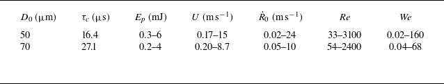


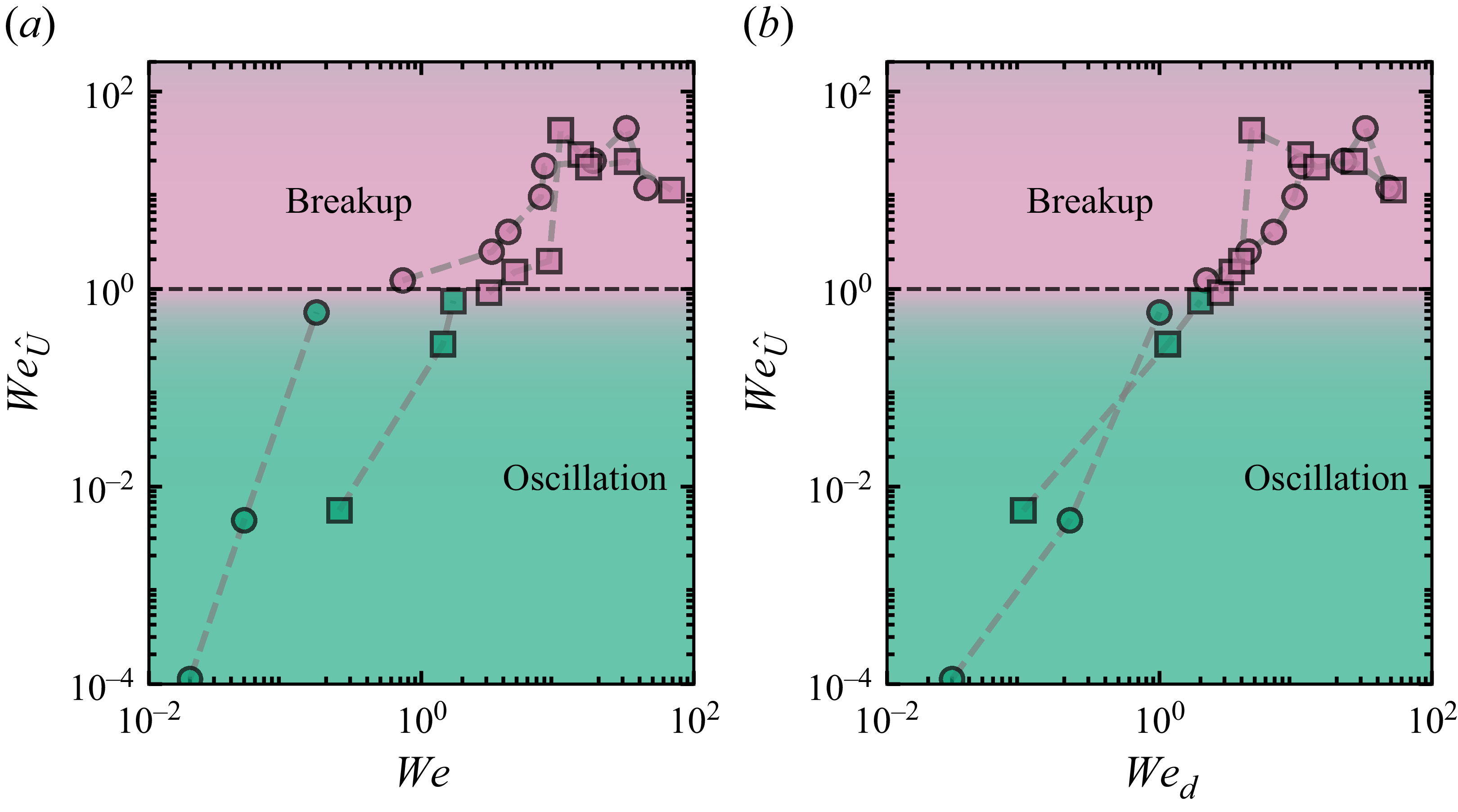


 Open access