


Introduction
Land-based ice is melting and raising global sea levels (Edwards et al., Reference Edwards, Nowicki, Marzeion, Hock, Goelzer, Seroussi and Jourdain2021), and the Greenland Ice Sheet is one of the leading contributors to global sea-level rise (IPCC, Reference Pörtner, Roberts, Masson-Delmotte, Zhai, Tignor, Poloczanska and Mintenbeck2019). The amount of sea-level rise from future retreat of the Greenland Ice Sheet is predicted from ice sheet models that consider different future warming scenarios (Goelzer et al., Reference Goelzer, Nowicki, Payne, Larour, Seroussi, Lipscomb and Gregory2020). To increase confidence in sea-level rise estimates, it is useful to compare ice sheet model output with geologic constraints of past ice sheet changes (Briner et al., Reference Briner, Cuzzone, Badgeley, Young, Steig, Morlighem and Schlegel2020). The Mid-Holocene (∼9–5 ka) is a geologically recent warm period often targeted to gauge ice sheet response to past warming because it is a partial analog for future warming (Axford et al., Reference Axford, de Vernal and Osterberg2021). Data-model comparisons during this time are difficult, because the ice sheet was smaller than at present in most areas between 6.5 ka and the Little Ice Age (1400–1850 CE) (Leger et al., Reference Leger, Clark, Huynh, Jones, Ely, Bradley, Diemont and Hughes2024). Reconstructions of relative sea level can track glacial isostatic adjustment through the entire Holocene, allowing for insights into glacial activity from 6.5 ka to the Little Ice Age (Antwerpen et al., Reference Antwerpen, Austermann, Young, Porter, Lewright and Latychev2024). These reconstructions can be directly compared with ice sheet model output to assess model fit or guide adjustments to learn about the ice-sheet history (Gowan, Reference Gowan2023). As there is spatial heterogeneity in glacial isostatic uplift patterns around Greenland, a dense network of sites is increasingly important to understand ice-sheet history (Long et al., Reference Long, Woodroffe, Roberts and Dawson2011).
Nares Strait is an area with spatial heterogeneity in the uplift pattern in part due to the convergence of the Greenland and Innuitian Ice Sheets. Here the marine limit varies along the axis of Nares Strait in a bullseye fashion (Long et al., Reference Long, Woodroffe, Roberts and Dawson2011), which is a pattern that is reproduced in glacial isostatic adjustment models (Lecavalier et al., Reference Lecavalier, Milne, Simpson, Wake, Huybrechts, Tarasov and Kjeldsen2014, Reference Lasher, Axford, McFarlin, Kelly, Osterberg and Berkelhammer2017). Despite the complicated pattern shown by the marine limit variability and glacial isostatic adjustment model output, the relative sea-level data are mostly limiting data: radiocarbon ages that require sea level to be at an unspecified height above the elevation of the sample (England, Reference England1985; Fredskild, Reference Fredskild1985; Funder, Reference Funder1990; Kelly and Bennike, Reference Kelly and Bennike1992; Bennike, Reference Bennike2002; Figs. 1 and 2). Elsewhere, data are considered sea level index points (SLIPs), which are typically radiocarbon ages that tie a specific elevation of a paleo–sea level height to a given time; SLIPs are typically derived from dated marine shells in marine deltas or terraces (Hall et al., Reference Hall, Baroni and Denton2010) or from isolation basin studies (e.g., Long et al., Reference Long, Woodroffe, Roberts and Dawson2011). Because this region has a gradient in sea-level history from SW to NE, and potentially an even more complicated sea level than the bullseye pattern, a SLIP-based study in the middle of Nares Strait helps the spatial distribution of sea-level data in the region and allows for a tighter window for models to target.
Northwest Greenland and Nares Strait. Individual sea level index points (SLIPs) are plotted as circles, and individual sea-level limits are plotted as triangles. Each study is assigned a different color. Large circles are groups of sea-level data that are plotted together in Figures 2, 5, and 6. The inset map shows the study area box in Greenland. The Greenland Ice Sheet, land elevation, and ocean bathymetry are from BedMachine v. 4 (Morlighem et al., Reference Morlighem, Williams, Rignot, An, Arndt, Bamber and Catania2017, Reference Morlighem, Williams, Rignot, An, Arndt, Bamber and Catania2021). Modern ice that is separate from the Greenland Ice Sheet is shown with the Randolph Glacier Inventory (RGI Consortium, 2023). Data are from Blake (Reference Blake1992), Funder (Reference Funder1990), Kelly et al. (Reference Kelly, Funder, Houmark-nielsen, Knudsen, Kronborg, Landvik and Sorby1999), Fredskild (Reference Fredskild1985), Weidick (Reference Weidick1977), Mason (Reference Mason2010), Nicholas (Reference Nichols1969), Bennike et al. (Reference Bennike2002), Glueder et al. (Reference Glueder, Mix, Milne, Reilly, Clark, Jakobsson, Mayer, Fallon, Southon and Padman2022), Kelly and Bennike (Reference Kelly and Bennike1992), and England (Reference England1985).

Regional sea-level data with estimated sea-level histories shown as solid and dashed lines. As in Figure 1, sea level index points (SLIPs) are circles, and sea-level limits are triangles. They are color coded by publication, as listed in the panels: Weidick (Reference Weidick1977); England (Reference England1985); Fredskild (Reference Fredskild1985); Funder (Reference Funder1990); Kelly and Bennike (Reference Kelly and Bennike1992); Bennike (Reference Bennike2002); and Glueder et al. (Reference Glueder, Mix, Milne, Reilly, Clark, Jakobsson, Mayer, Fallon, Southon and Padman2022). Our study site lies between Inglefield Fjord and Washington Land. The marine limit is plotted as a solid black line with the elevation labeled above it. Washington and Hall Land have two plots each. The plots labeled “Raw Elevations” have Glueder et al. (Reference Glueder, Mix, Milne, Reilly, Clark, Jakobsson, Mayer, Fallon, Southon and Padman2022) samples as minimum limits, and they are plotted as red triangles with their raw elevations (using collection elevation instead of adjusted elevation). The plots labeled “Habitat Correction” have Glueder et al. (Reference Glueder, Mix, Milne, Reilly, Clark, Jakobsson, Mayer, Fallon, Southon and Padman2022) samples as SLIPs as red circles and are plotted with their habitat-corrected depths. Glueder et al. (Reference Glueder, Mix, Milne, Reilly, Clark, Jakobsson, Mayer, Fallon, Southon and Padman2022) habitat-corrected model output shown with uncertainty.

Glueder et al. (Reference Glueder, Mix, Milne, Reilly, Clark, Jakobsson, Mayer, Fallon, Southon and Padman2022) recently produced a relative sea level reconstruction using marine bivalves from raised marine deposits with a novel δ18O-based habitat depth relationship in Hall Land and Washington Land (Figs. 1 and 2). Using their relative sea level reconstruction, Glueder et al. (Reference Glueder, Mix, Milne, Reilly, Clark, Jakobsson, Mayer, Fallon, Southon and Padman2022) tested ice-history scenarios and interpreted a Middle Holocene sea-level standstill being caused by hundreds of meters of ice-cap growth from 6 to 2 ka, followed by sea-level fall from 2 ka to the present due to subsequent ice-cap disappearance. This inferred ice-cap history challenges field data from the nearby Petermann and Humbolt Glaciers that were advancing through the Neoglacial and Little Ice Age, reaching near the present margin at least 2.8 ± 0.3 ka and followed by a regionally maximum Late Holocene extent ∼300 ± 200 years ago (Reusche et al., Reference Reusche, Marcott, Ceperley, Barth, Brook, Mix and Caffee2018). Additionally, the coolest part of the Holocene following the thermal maximum is recorded in the last millennium in lake records from Pituffik to Inglefield Land (Blake et al., Reference Blake, Boucherle, Fredskild, Janssens and Smol1992; Briner et al., Reference Briner, McKay, Axford, Bennike, Bradley, de Vernal and Fisher2016; Lasher et al., Reference Lasher, Axford, McFarlin, Kelly, Osterberg and Berkelhammer2017; Axford et al., Reference Axford, Lasher, Kelly, Osterberg, Landis, Schellinger, Pfeiffer, Thompson and Francis2019). This pattern of decreasing temperature through the Middle and Late Holocene and into the Little Ice Age is found in all sectors of Greenland (Kjær et al., Reference Kjær, Bjørk, Kjeldsen, Hansen, Andresen, Siggaard-Andersen and Khan2022). Additional SLIPs from this region could help clarify the Holocene sea level and ice-loading history in northwestern Greenland.
We present a new relative sea level curve based on SLIPs and limiting data from a flight of raised marine terraces on Inglefield Land, northwest Greenland, to fill a spatial data gap and help understand the history of ice loading. We find that the Inglefield Land coastline deglaciated before 9010–8650 cal yr BP, and the land emerged at a rate of 49 m/ka between 9010–8650 and 7970–7790 cal yr BP. After 7970–7790 cal yr BP, emergence slowed to 11 m/ka until ∼5000, whereupon sea level likely then fell continuously to the present.
Study area
In northwest Greenland, the Greenland and Innuitian Ice Sheets converged in Nares Strait during the last glacial maximum, flowing southward into Baffin Bay and northward into the Arctic Ocean (England, Reference England1999; Couette et al., Reference Couette, Lajeunesse, Ghienne, Dorschel, Gebhardt, Hebbeln and Brouard2022; Batchelor et al., Reference Batchelor, Krawczyk, O’Brien and Mulder2024). The oldest marine bivalves are 10,700–9720 and 10,370–9440 cal yr BP from Pituffik and Hall Land, respectively, and 7920–7450 cal yr BP from southwest Washington Land (England, Reference England1985; Kelly et al., Reference Kelly, Funder, Houmark-nielsen, Knudsen, Kronborg, Landvik and Sorby1999; Bennike, Reference Bennike2002; see Fig. 1 for locations). The marine limit increases from 40 m above sea level (m asl) near Pituffik to 124 m asl in Hall Land (Nichols, Reference Nichols1969; Kelly and Bennike, Reference Kelly and Bennike1992; Bennike, Reference Bennike2002; Fig. 2). In Hall Land and Washington Land, the land emergence was slow in the beginning, rapid in the Mid-Holocene, and slowed to the present (England, Reference England1985; Kelly and Bennike, Reference Kelly and Bennike1992; Bennike, Reference Bennike2002). In Inglefield Fjord and Pituffik, land emergence was rapid before slowing to the present, although there are fewer data to constrain this pattern (Fredskild, Reference Fredskild1985; Funder, Reference Funder1990; Kelly et al., Reference Kelly, Funder, Houmark-nielsen, Knudsen, Kronborg, Landvik and Sorby1999). These patterns together likely reflect the “unzipping” of the two coalesced ice sheets (England, Reference England1999).
The glacial history of Inglefield Land is well known from sediment cores, radiocarbon dating of reworked marine bivalves, and cosmogenic nuclide exposure dating. Sediment cores from Kane Basin, offshore of Inglefield Land, record deglaciation before 9000–8300 cal yr BP (Georgiadis et al., Reference Georgiadis, Giraudeau, Martinez, Lajeunesse, St-Onge, Schmidt and Massé2018). Nichols (Reference Nichols1969) described the geomorphology of Inglefield Land and investigated both the raised beach deposits adjacent to our study area in Rensselaer Bay and the raised marine deltas across the river from our study site; a radiocarbon date on peat constrains deglaciation of the coastline in Rensselaer Bay to before 9130–8180 cal yr BP. Søndergaard et al. (Reference Søndergaard, Larsen, Steinemann, Olsen, Funder, Egholm and Kjær2020) used cosmogenic nuclide exposure dating and radiocarbon dating of reworked marine bivalves to show the ice sheet reached its present margin by 6.7 ± 0.3 ka and was smaller than present from sometime before 5930–5750 to 600–500 cal yr BP. Mason (Reference Mason2010) investigated a suite of raised beaches at Cape Grinnell (∼20 km northeast of our study site) and inferred sea level fell rapidly at Cape Grinnell from the 72 m asl marine limit to approximately 20 m asl, when a short standstill occurred, followed by a fall to around 5 m, where he inferred a transgression occurred, before sea level fell to the present. Mason (Reference Mason2010) added age control to his work with radiocarbon ages from marine bivalves reworked in solifluction lobes and from within beach ridges (minimum ages) and ages on caribou and muskox bone from Thule settlement remains that constrain sea level to a lower elevation (maximum ages). Finally, a well-constrained relative sea level curve from Cape Hershel, Ellesmere Island, 90 km due west and across Nares Strait from our study site, shows rapid sea-level fall along the Ellesmere Island coast after deglaciation at 8300–9000 cal yr BP and a steady fall to the present (Blake, Reference Blake1992).
Methods
We investigated six raised marine terraces along the west side of the Rensselaer River. These terraces formed when delta deposition ended as glacial isostatic adjustment uplifted the delta above the ocean surface, and the river eroded through the paleo-delta deposit to the new base level (Fig. 3). We measured the elevation of terrace surfaces and targeted sediment exposures that contained material for radiocarbon dating (Fig. 4). Radiocarbon ages on plant and marine bivalve samples are used to determine the timing of delta progradation and define the timing of sea level at the elevation of the topset/foreset contact.
Polar Geospatial Center 0.5 m imagery of Rensselaer Bay. Raised terraces along the west side of the river are labeled, and blue circles indicate radiocarbon samples. Imagery © 2021 Maxar.

Field images of raised terraces and example radiocarbon samples. (A) Overview of Rensselaer Bay from above showing the modern river and delta (center) and Terraces 2–6 (left of river). (B) Terrace 5 at 39 ± 4 m asl. Person for scale at sampling location—foreset beds are shown in cross section, and topset gravel beds covered in colluvium. (C) Terrace 6 at 10 ± 4 m asl. This shows the dipping foreset beds and the modern river on the right. (D) Terraces 2 and 3 at 66 ± 4 and 52 ± 4 m asl, respectively. Some foreset beds can be seen behind the footprints. (E) Salix stem from Terrace 6 (sample 22GROm-08; 5320-5060 cal yr BP). (F) Articulated marine bivalve within the foreset beds of Terrace 2 (sample 22GROm-01; 8900–8160 cal yr BP). (G) Terrestrial Calligeron sp. mosses protruding from the foreset beds in Terrace 3 (sample 22GROm-04; 9010–8650 cal yr BP).

Table 1 reports the terrace surface elevation estimations and the relationship between the radiocarbon sample locations and past sea level. In the field, we determined the elevation of terraces surface using a handheld GPS. Similar to our handheld GPS, ArcticDEM reports elevation in meters above the WGS 84 ellipsoid with a ±4 m uncertainty across the entire product (Porter et al., Reference Porter, Howat, Noh, Husby, Khuvis, Danish and Tomko2023). We use the ArcticDEM to reduce uncertainties. We averaged five elevation points on each terrace spaced out along the northern end of the terrace, which was the seaward-facing end. On average, the reported present sea surface height above the ellipsoid in this area is 11 ± 0.1 m. We subtract this from the terrace and sample elevation to report terrace elevation in meters above sea level (m asl).
Terrace elevation data.

a SLIP, sea level index point.
In the University at Buffalo Glacial History Laboratory, we rinsed marine bivalve shells with deionized water to remove sediment, scraped away friable outer layers of the shells with forceps, and freeze-dried them. For radiocarbon dating, we targeted the shell umbo, because it is the thickest part of the shell and harder to contaminate than the thin edges (e.g., Hall et al., Reference Hall, Baroni and Denton2010). We rinsed terrestrial macrofossils with deionized water then freeze-dried single Calligeron sp. moss strands and a Salix sp. stem. We sent samples to the National Ocean Sciences Accelerated Mass Spectrometry (NOSAMS) Laboratory for radiocarbon dating. NOSAMS performed acid-base-acid (ABA) pretreatments before converting samples to graphite and running them on the accelerated mass spectrometer (Vogel et al., Reference Vogel, Southon, Nelson and Brown1984; Pearson et al., Reference Pearson, McNichol, Schneider, Von Reden and Zheng1997; Shah Walter et al., Reference Shah Walter, Gagnon, Roberts, McNichol, Gaylord and Klein2015; Elder et al., Reference Elder, Roberts, Walther and Xu2019). The δ13C was measured on an isotope-ratio mass spectrometer using the CO2 from each sample; uncertainties are <0.1‰, and we report δ13C values as ‰ VPDB.
Table 2 reports radiocarbon data and ages; in the text we report the maximum and minimum of the 2-sigma age range. We used Calib8.1 with the IntCal20 dataset to calibrate terrestrial samples (Stuiver and Reimer, Reference Stuiver and Reimer1993; Reimer et al., Reference Reimer, Austin, Bard, Bayliss, Blackwell, Bronk Ramsey and Butzin2020). We radiocarbon dated marine bivalves from five of the six terraces, and terrestrial and marine sample pairs from three of the six terraces. We used the online DeltaR application (http://calib.org/deltar) to calculate the ΔR for these sample pairs (Reimer and Reimer, Reference Reimer and Reimer2017). This technique uses the calibrated age of the terrestrial sample to predict a contemporaneous uncalibrated marine age—the difference between this prediction and the measured uncalibrated marine 14C age is the ΔR and includes the uncertainty from both terrestrial and marine samples (Reimer and Reimer, Reference Reimer and Reimer2017). Our two samples that are not paired with a terrestrial sample (22GROm-1 and 9) are similar in age to one of our paired samples (22GROm-4 and 6), and so we apply this ΔR with Marine20 in Calib8.1 to calibrate the marine bivalve ages (Reimer and Reimer, Reference Reimer and Reimer2017; Heaton et al., Reference Heaton, Köhler, Butzin, Bard, Reimer, Austin, Ramsey, Grootes, Hughen and Kromer2020; Table 2). We speculate that an embayment with local and variable freshwater input could lead to variable ΔR through time and differences with ΔR from elsewhere, so we assume our local ΔR constraints are more accurate than using the ΔR reported for the Canadian Arctic Archipelago (Pieńkowski et al., Reference Pieńkowski, Coulthard and Furze2023).

Supplementary Tables 1–3 supply the information to recalculate our radiocarbon ages as well as the compiled regional ages shown in Figures 1, 2, 5, and 6 and Table 2. Regional data are recalculated with IntCal20 and Marine 20 in Calib8.1 (Heaton et al., Reference Heaton, Köhler, Butzin, Bard, Reimer, Austin, Ramsey, Grootes, Hughen and Kromer2020; Reimer et al., Reference Reimer, Austin, Bard, Bayliss, Blackwell, Bronk Ramsey and Butzin2020) with the ΔR of 188 ± 91 14C yr BP, as suggested for northwestern Canadian Arctic Archipelago (Pieńkowski et al., Reference Pieńkowski, Coulthard and Furze2023). We calculate a local ΔR and apply this to the radiocarbon ages for the Mason (Reference Mason2010) Early Holocene marine bivalves, because they lived in similar space (<20 km away) and time (∼9000–8000 yr BP) as our ΔR reconstructions. Using the Pieńkowski et al. (Reference Pieńkowski, Coulthard and Furze2023) ΔR value instead would shift ages 400 years younger at most and does not change our results or interpretations (Supplementary Table 5). We depict the most likely relative sea-level history with a line from the marine limit, above the limiting data, through the SLIPs, and to the present. We compare our data with regional sea-level histories illustrated in similar fashion, except for sea-level histories from Glueder et al. (Reference Glueder, Mix, Milne, Reilly, Clark, Jakobsson, Mayer, Fallon, Southon and Padman2022), which include an error-in-variables modeling approach to predict the sea-level history (Cahill et al., Reference Cahill, Kemp, Horton and Parnell2015).
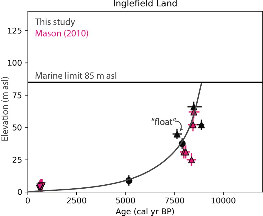
The radiocarbon ages from Inglefield Land plotted against elevation. The marine limit is the solid black line at 85 m. New minimum-limiting constraints are shown by upward-facing black triangles. New sea level index points (SLIPs) are shown by black circles. Relative sea-level history drawn through the SLIPs and estimated from 5000 cal yr BP to the present. Mason (Reference Mason2010) data are shown in pink, with minimum limits as upward triangles and maximum limits as downward triangles.

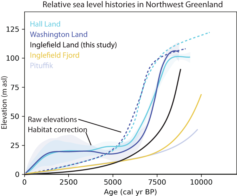
Combined relative sea level histories from Pituffik to Hall Land. Colors are the same as in Figures 1 and 2. The solid teal curve with uncertainty is the relative sea level history proposed from Glueder et al. (Reference Glueder, Mix, Milne, Reilly, Clark, Jakobsson, Mayer, Fallon, Southon and Padman2022) for Hall Land. The solid purple curve with uncertainty is the same as the teal curve but for Washington Land. The dashed teal and purple curves are sea-level histories drawn for Hall Land and Washington Land when data from Kelly and Bennike (Reference Kelly and Bennike1992), England (Reference England1985), Bennike (Reference Bennike2002), and Glueder et al. (Reference Glueder, Mix, Milne, Reilly, Clark, Jakobsson, Mayer, Fallon, Southon and Padman2022) are all drawn as minimum-limiting data (i.e., the raw elevation from Glueder et al. [Reference Glueder, Mix, Milne, Reilly, Clark, Jakobsson, Mayer, Fallon, Southon and Padman2022]). The dashed lines are the same as the raw elevation plots of Hall Land and Washington Land from Figure 2. The black curve is from this study. The yellow curve is estimated from Inglefield Fjord (Fredskild, Reference Fredskild1985). The light purple curve is estimated from Pituffik (Funder, Reference Funder1990).

Results
The terraces we sampled from are composed of silty and sandy foreset beds containing both articulated marine bivalves and terrestrial macrofossils, which are overlain by horizontal gravelly topset beds with occasional boulders on terrace surfaces (Fig. 4). In some places, terrace surfaces contain storm beach berms. The presence of steeply dipping foreset and subhorizontal topset beds are characteristic of Gilbert-style deltas where past sea-level elevation is interpreted to be at the foreset/topset contact (Gilbert, Reference Gilbert1890). We found this contact to be within 1 to 2 m of terrace surfaces.
Tables 1 and 2 and Figure 5 show the elevation–age relationship of the marine terraces we sampled. Terrace 1, the highest terrace, has a surface elevation of 85 ± 4 m asl. We were unable to expose sediments here and did not find material for radiocarbon dating. In Terrace 2 (surface at 66 ± 4 m asl), we collected an articulated Hiatella arctica shell from foreset beds that dates to 8900–8160 cal yr BP. We sampled an articulated Astarte borealis shell and Calligeron sp. moss from the foreset beds of Terrace 3 (52 ± 4 m asl); the Calligeron moss dates to 9010–8650 cal yr BP. From Terrace 4 (45 ± 4 m asl), we sampled an unidentifiable shell fragment from a shallow pit (<1 m) that we dug into the terrace surface that dates to 7880–7400 cal yr BP; there were no natural exposures in this terrace level. Terrace 5 is at 39 ± 4 m asl, where a 1.5-m-thick cobble-rich topset bed overlies foreset beds; the edge of this terrace has an ∼1-m-high beach ridge. We sampled an articulated Mya truncata bivalve and Calligeron sp. moss from the foreset beds ∼1 m beneath the topset beds; the Calligeron moss dates to 7970–7790 cal yr BP. Finally, Terrace 6 is at 10 ± 4 m asl, where a <1-m-thick topset bed caps the terrace. We sampled an articulated Mya truncata bivalve and Salix sp. stem from the foreset beds; the Salix stem dates to 5320–5060 cal yr BP. The ΔR from the 52 ± 4, 39 ± 4, and 10 ± 4 m asl terrace sample pair is −123 ± 135, 29 ± 104, and −35 ± 125 14C yr BP, respectively.
Interpretation
Because we found no marine bivalves associated with Terrace 1 at 85 ± 4 m asl and there was no natural exposure of this terrace, we do not know if this terrace is a remnant of a fluvial terrace that graded to a marine limit or if this terrace is a marine delta formed with the marine limit. We interpret the sea-level height associated with this terrace to have been 85 ± 4 m asl or lower. The oldest age from our analysis, from Terrace 3, is the closest constraint on the marine limit, so we assign 9010–8650 cal yr BP as our closest minimum-limiting constraint on both deglaciation and the marine limit.
Nichols (Reference Nichols1969) noted that some terraces in Rensselaer Valley have foreset beds that extend to the top of the terrace. They explained this observation as fluvial erosion of previously deposited (higher-elevation) marine deltas and removal of the topset bed and some amount of the foreset beds. If this were the case, samples from such foreset beds would be unrelated to the current (strath) terrace surface elevation and the age associated with a higher relative sea level. However, if the upper terrace sediments were indeed planed off from fluvial erosion, subhorizontal fluvial deposits associated with river deposition (which would appear as topset beds) might be expected, but these were not observed. In any case, we find it safest to interpret radiocarbon ages from terraces lacking topset beds as underestimating sea-level elevation at that time and use them as minimum constraints.
We found that Terrace 2 at 66 ± 4 m asl lacks topset beds and has foreset beds that extend to the surface; therefore, we use this sample as a minimum constraint. The terrestrial sample from Terrace 3 (52 ± 4 m asl; 9010–8650 cal yr BP) is the same age within uncertainty as the marine bivalve from Terrace 2 (8900–8160 cal yr BP). It is possible that the surface at 52 ± 4 m may be a strath terrace cut into older marine delta sediments. Because we are unsure, we consider this sample a minimum constraint on sea level as well and plot Terraces 2 and 3 in Figure 5 by their terrace elevation (Table 1). However, because it appears sea level was falling rapidly at this time, these ages are likely to be very close minimums on sea-level elevation.
The ages from Terraces 4 and 5 (45 ± 4 m asl; 7880–7400 cal yr BP; and 39 ± 4 m asl; 7970–7790 cal yr BP) overlap within uncertainty, but the Terrace 4 sample is likely out of stratigraphic order. The Terrace 4 sample is a single fragment found in a shallow pit and may not be in situ, so we believe it has a reasonable chance of upslope reworking from birds or wind. Therefore, we do not use the sample from Terrace 4 in our relative sea-level analysis and label the sample “float” in Figure 5.
We have confidence that the Terrace 5 radiocarbon sample (39 ± 4 m asl; 7970–7790 cal yr BP) is a SLIP, because there is an identifiable topset/foreset contact in the terrace and a beach berm preserved on the outer edge of the terrace surface. Finally, Terrace 6 has a topset/foreset contact, so we also interpret this radiocarbon age and elevation as a SLIP (10 ± 4 m asl; 5320–5060 cal yr BP). In Figure 5, these data points are plotted as SLIPs with the elevation of the topset/foreset contact.
Discussion
The pattern of Holocene sea-level change
The timing of deglaciation in Inglefield Land agrees with prior reconstructions of the unzipping of the two coalesced ice sheets. Our oldest terrestrial radiocarbon date of 9010–8650 cal yr BP lies between the oldest dates from Inglefield Fjord (9760–8910 cal yr BP) and southwest Washington Land (7920–7450 cal yr BP; Fredskild, Reference Fredskild1985; Bennike, Reference Bennike2002). The date also agrees with sediment cores from Kane Basin in southern Nares Strait, ∼100 km due north of our study site, that constrain deglaciation to ∼8900–8560 cal yr BP (Georgiadis et al., Reference Georgiadis, Giraudeau, Martinez, Lajeunesse, St-Onge, Schmidt and Massé2018) and peat from marine terraces in Rensselaer Valley of 9130–8180 cal yr BP (Nichols, Reference Nichols1969).
In Rensselaer Valley, sea level fell rapidly from the marine limit to our first SLIP from 9010–8650 to 7970–7790 cal yr BP at a rate of 49 m/ka. The rate of sea-level fall slowed to 11 m/ka between our two SLIPs at 7970–7790 and 5320–5060 cal yr BP. After 5320–5060 cal yr BP, our best estimate of steady sea-level fall to the present results in a decrease to 2 m/ka. Our data indicate thick last glacial maximum ice over our study area; sea level fell rapidly between the marine limit and the first SLIP ∼8000 cal yr BP, showing that the land was rebounding quickly upon deglaciation.
There is conflicting evidence from Mason (Reference Mason2010) and Nichols (Reference Nichols1969) about evidence of standstills in the geomorphology of the beach ridges at Rensselaer Bay. Mason (Reference Mason2010) described the beaches in Cape Grinnell (Fig. 1) and interpreted a sea-level standstill at 20 m asl and a short-lived transgression at 5 m asl. If we use our relative sea level reconstruction between 8000 and 5000 cal yr BP (from SLIPs), such a 20 m standstill would have occurred ∼6200 cal yr BP. Such a sea-level oscillation at 5 m asl would have occurred ∼3700 cal yr BP. Sea level had five more meters to fall between this standstill and present sea level between 3700 cal yr BP and the present. If this transgression did last multiple millennia, sea level had to fall five more meters to intersect modern sea level, and this would cause rapid sea-level fall during the coldest interval in north Greenland, and challenge the regional ice histories (e.g., of Ruesch et al., Reference Reusche, Marcott, Ceperley, Barth, Brook, Mix and Caffee2018). The possibility of a Late Holocene standstill is also challenged by the geomorphology reported by Nichols (Reference Nichols1969), who interpreted steady sea-level fall from the marine limit to present from beach ridges 4 km from our study site. Continuous sea-level fall shown by Nichols (Reference Nichols1969) does not rule out a J-shape sea-level curve, in which sea level falls below present and rises the equivalent to present sea level (Long et al., Reference Long, Woodroffe, Dawson, Roberts and Bryant2009). The beach ridges closest to the ocean could be, for example, ∼4000–3000 years old and sea level could have risen from a low point to the modern elevation after ∼2000–1000 years ago. Neither of these publications nor our own, however, have age control after 5000 cal yr BP. Thus, more attention to raised terraces between 10 m asl and present sea level would help reconcile the relative sea-level history in the Middle and Late Holocene.
Figure 6 shows that the sea-level history of Inglefield Land captures the transition between the style of emergence in southern and northern Nares Strait. Supplementary Table 4 supplies information to calculate regional rates of sea level change. Even though there are few data to constrain the curves drawn in Figure 6 from Inglefield Fjord and Pituffik, the general trend of the decreasing marine limits from Pituffik to Hall Land shows the influence of the increased ice load in the center of Nares Strait. While Washington and Hall Land have higher marine limits, constraints show a slow rate (5 m/ka and 3 m/ka, respectively) of emergence after deglaciation that leads to lower rates overall. This delay in the emergence rate may be from slower ice retreat when those sites were initially deglaciated. Washington and Hall Land have their highest rates of sea level fall between ∼7.6 and 5 cal ka BP (30 m/ka) and ∼8.4 and 5.8 cal ka BP (34 m/ka). Inglefield Fjord had the highest rate of emergence during the same time as Inglefield Land, with a rate of 30 m/ka between ∼9.4 and 7.6 cal ka BP. Finally, Pituffik has the lowest rate of emergence of 6 m/ka between ∼10.5 and 7 cal ka BP, also during the same time as Inglefield Fjord and Inglefield Land. This pattern is consistent with increasing ice loading and decreasing deglaciation age toward the middle of Nares Strait.
Figure 6 shows the difference between the sea-level histories for Hall Land and Washington Land with and without the habitat correction employed by Glueder et al. (Reference Glueder, Mix, Milne, Reilly, Clark, Jakobsson, Mayer, Fallon, Southon and Padman2022). The habitat-corrected sea-level data, which indicate a sea-level standstill from 6 to 2 ka, appear anomalous in the context of other records (solid teal and purple lines in Fig. 6). However, if the shell data are instead considered raw (using collection elevation instead of adjusted elevation) and hence are relative sea level minimums, the relative sea level histories are highly compatible (dashed teal and purple lines in Fig. 6). Additionally, because the habitat-corrected sea-level history is explained by an anomalous ice history compared with the rest of Greenland, we find this to be an added reason to favor the relative sea level curves based on the raw shell data.
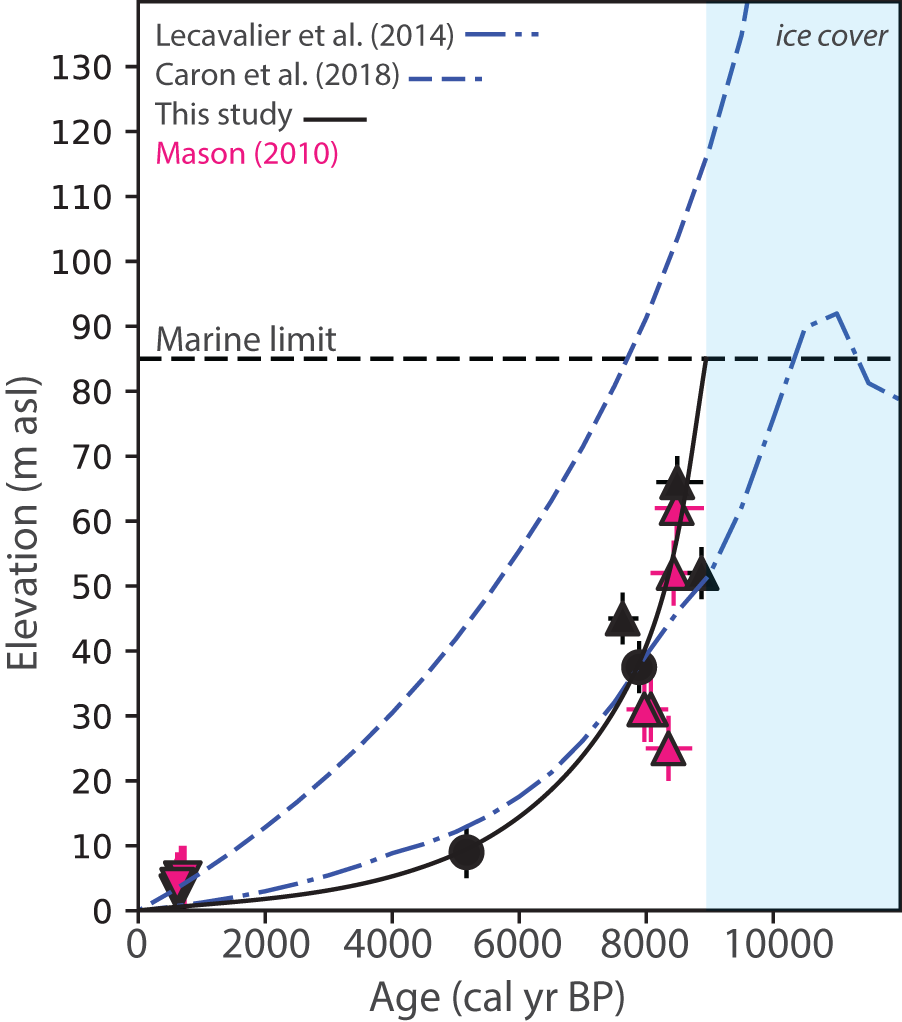
To investigate our reconstruction further, we compare our sea-level curve with model predictions from a regional glacial isostatic adjustment model (Huy3; Lecavalier et al., Reference Lecavalier, Milne, Simpson, Wake, Huybrechts, Tarasov and Kjeldsen2014) and a global glacial isostatic adjustment model (Caron et al., Reference Caron, Ivins, Larour, Adhikari, Nilsson and Blewitt2018) (Fig. 7). We find that Huy3 model output has an earlier deglaciation timing than our data support, leading to a 92 m asl marine limit at ∼11,000 cal yr BP. We measured an 85 ± 4 m asl marine limit that dates to ∼9000 cal yr BP—a difference of only 4 m, within the uncertainty of our measurement. The early simulated deglaciation leads to sea level lowering earlier than in our reconstruction. If simulated deglaciation occurred 2000 years, the model would likely match our sea-level reconstruction even more closely. The Lecavalier et al. (Reference Lecavalier, Milne, Simpson, Wake, Huybrechts, Tarasov and Kjeldsen2014) model matches our 8000 and 5000 cal yr BP SLIPs. This reasonably good data-model fit from deglaciation to 5000 cal yr BP supports our interpolation between 5000 and the present despite the lack of data constraints in this interval. The Caron et al. (Reference Caron, Ivins, Larour, Adhikari, Nilsson and Blewitt2018) model simulates deglaciation even earlier than Huy3 (12,500 years ago), which explains their 253 m asl marine limit. This model also predicts steady sea-level fall from deglaciation to the present without a standstill or a J-shape. Thus, both the available modeling and the trajectory of our data support a smoothly declining sea-level height between 5000 cal yr BP and the present.
Data-model comparison between relative sea level reconstruction in this study and glacial isostatic adjustment model predictions of relative sea level for our study site. The blue dash-dot curve is from Lecavalier et al. (Reference Lecavalier, Milne, Simpson, Wake, Huybrechts, Tarasov and Kjeldsen2014). The blue dashed curve is from Caron et al. (Reference Caron, Ivins, Larour, Adhikari, Nilsson and Blewitt2018). Our reconstruction is shown with black triangles for limiting data and black circles for sea level index points (SLIPs). Data from Mason (Reference Mason2010) are shown as upward and downward pink triangles for minimum- and maximum-limiting constraints, respectively. The blue shaded box indicates when Rensselaer Valley was covered with ice (until ∼9 ka).

These modeled glacial isostatic adjustment predictions of steady sea-level fall to the present likely arise from the fact that neither considers a change in the ice margin from 7 ka to the present (Lecavalier et al., Reference Lecavalier, Milne, Simpson, Wake, Huybrechts, Tarasov and Kjeldsen2014; Caron et al., Reference Caron, Ivins, Larour, Adhikari, Nilsson and Blewitt2018). We know from reworked bivalves in Humbolt Glacier Little Ice Age moraines that the ice sheet was somewhere behind its present margin during the Middle–Late Holocene (Søndergaard et al., Reference Søndergaard, Larsen, Steinemann, Olsen, Funder, Egholm and Kjær2020). The Middle–Late Holocene ice growth may have impacted the sea-level history if the scale of loading was large enough to influence the solid Earth. Glueder et al. (Reference Glueder, Mix, Milne, Reilly, Clark, Jakobsson, Mayer, Fallon, Southon and Padman2022) showed there needed to be a thinner lithosphere and less viscous mantle than that originally proposed for Greenland (Lecavalier et al., Reference Lecavalier, Milne, Simpson, Wake, Huybrechts, Tarasov and Kjeldsen2014) to obtain their derived standstill in sea-level history. This indicates the solid Earth in northwest Greenland, with the optimally fit Earth parameters, may not be sensitive to smaller-scale ice growth-and-retreat cycles.
Conclusions
This new relative sea level curve from Inglefield Land supplements the available sea-level histories along Nares Strait, northwest Greenland, with new limiting and SLIP data. Our results show that the coast of Inglefield Land deglaciated by 9010–8650 cal yr BP, and sea level fell rapidly at a rate of 49 m/ka until 7970–7790 cal yr BP. Emergence decreased first to 11 m/ka until 5320–5060 before likely decreasing to 2 m/ka through to the present. This new sea-level history captures the transition from the style of emergence at either end of the Nares Strait: from Pituffik to Hall Land, the rate of emergence generally increases, while the period of fastest emergence is younger. This reconstruction estimates steady sea-level fall from 5000 years ago to the present, which is supported by glacial isostatic adjustment model predictions. This history agrees with the pattern of sea-level fall after ∼5000 cal yr BP when using the raw (noncorrected) elevations from Glueder et al. (Reference Glueder, Mix, Milne, Reilly, Clark, Jakobsson, Mayer, Fallon, Southon and Padman2022). Future work should investigate the post–5000 year history to fully determine the evidence for standstill/J-shape and the implications for the ice history; additional SLIPs from the abundant marine deltas in other river valleys in Inglefield Land would be most useful. These data can be used to benchmark ice-sheet and glacial isostatic adjustment models in an area with a high degree of spatial heterogeneity in sea-level history.
Supplementary material
The supplementary material for this article can be found at https://doi.org/10.1017/qua.2025.10049.
Acknowledgments
We thank Caleb Walcott-George and Joerg Schaefer for help and good company in the field. Thanks to the staff at Battelle, U.S. National Science Foundation, and the U.S. Air Mobility Command for logistical and field support. Thanks to AirGreenland for helicopter support. Much gratitude to Ole Bennike for helping with macrofossil identification. Thanks to Glenn Milne and Lambert Caron for providing glacial isostatic adjustment model output. Geospatial support for this work was provided by the Polar Geospatial Center under U.S. National Science Foundation–Office of Polar Programs awards 1043681, 1559691, and 2129685. Digital elevation models (DEMs) provided by the Polar Geospatial Center under NSF-OPP awards 1043681, 1559691, 1542736, 1810976, and 2129685. This work was funded by the U.S. National Science Foundation grant no. 2106971. Finally, we thank two anonymous reviewers and associate editor T. Lowell for detailed reviews that improved this article.
Competing Interests
The authors declare no competing interests.


 Open access