


Impact Statement
Methane is a potent greenhouse gas, making accurate monitoring of its sources essential for effective climate action. This study presents a framework that integrates drone-based measurements with artificial intelligence to improve the detection and quantification of methane emissions. By combining Bayesian inference with atmospheric dispersion modeling and drone-based atmospheric data, the system estimates source locations and emission rates. Reinforcement learning enables the drone to plan adaptive flight paths that maximize information gain in unfamiliar environments. This framework supports the development of intelligent, efficient tools for environmental monitoring, with applications in climate science, emissions reporting, and regulatory compliance.
1. Introduction
Methane (CH $ {}_4 $
) is an important greenhouse gas emitted by a range of anthropogenic activities, including fossil fuel extraction, agriculture, and waste management, as well as natural sources such as inland waters, wild animals, and thawing permafrost (IPCC, Reference Lee and Romero2023). Accurate quantification of CH
$ {}_4 $
) is an important greenhouse gas emitted by a range of anthropogenic activities, including fossil fuel extraction, agriculture, and waste management, as well as natural sources such as inland waters, wild animals, and thawing permafrost (IPCC, Reference Lee and Romero2023). Accurate quantification of CH $ {}_4 $
emissions are essential for climate change mitigation; yet, current national and global inventories remain highly uncertain (Saunois et al., Reference Saunois, Stavert, Poulter, Bousquet, Canadell, Jackson, Raymond, Dlugokencky, Houweling, Patra, Ciais, Arora, Bastviken, Bergamaschi, Blake, Brailsford, Bruhwiler, Carlson, Carrol, Castaldi, Chandra, Crevoisier, Crill, Covey, Curry, Etiope, Frankenberg, Gedney, Hegglin, Höglund-Isaksson, Hugelius, Ishizawa, Ito, Janssens-Maenhout, Jensen, Joos, Kleinen, Krummel, Langenfelds, Laruelle, Liu, Machida, Maksyutov, McDonald, McNorton, Miller, Melton, Morino, Müller, Murguia-Flores, Naik, Niwa, Noce, O’Doherty, Parker, Peng, Peng, Peters, Prigent, Prinn, Ramonet, Regnier, Riley, Rosentreter, Segers, Simpson, Shi, Smith, Steele, Thornton, Tian, Tohjima, Tubiello, Tsuruta, Viovy, Voulgarakis, Weber, Van Weele, Van Der Werf, Weiss, Worthy, Wunch, Yin, Yoshida, Zhang, Zhang, Zhao, Zheng, Zhu, Zhu and Zhuang2020). As identified by Saunois et al. (Reference Saunois, Martinez, Poulter, Zhang, Raymond, Regnier, Canadell, Jackson, Patra, Bousquet, Ciais, Dlugokencky, Lan, Allen, Bastviken, Beerling, Belikov, Blake, Castaldi, Crippa, Deemer, Dennison, Etiope, Gedney, Höglund-Isaksson, Holgerson, Hopcroft, Hugelius, Ito, Jain, Janardanan, Johnson, Kleinen, Krummel, Lauerwald, Li, Liu, McDonald, Melton, Mühle, Müller, Murguia-Flores, Niwa, Noce, Pan, Parker, Peng, Ramonet, Riley, Rocher-Ros, Rosentreter, Sasakawa, Segers, Smith, Stanley, Thanwerdas, Tian, Tsuruta, Tubiello, Weber, Van Der Werf, Worthy, Xi, Yoshida, Zhang, Zheng, Zhu, Zhu and Zhuang2024), increasing the density of CH
$ {}_4 $
emissions are essential for climate change mitigation; yet, current national and global inventories remain highly uncertain (Saunois et al., Reference Saunois, Stavert, Poulter, Bousquet, Canadell, Jackson, Raymond, Dlugokencky, Houweling, Patra, Ciais, Arora, Bastviken, Bergamaschi, Blake, Brailsford, Bruhwiler, Carlson, Carrol, Castaldi, Chandra, Crevoisier, Crill, Covey, Curry, Etiope, Frankenberg, Gedney, Hegglin, Höglund-Isaksson, Hugelius, Ishizawa, Ito, Janssens-Maenhout, Jensen, Joos, Kleinen, Krummel, Langenfelds, Laruelle, Liu, Machida, Maksyutov, McDonald, McNorton, Miller, Melton, Morino, Müller, Murguia-Flores, Naik, Niwa, Noce, O’Doherty, Parker, Peng, Peng, Peters, Prigent, Prinn, Ramonet, Regnier, Riley, Rosentreter, Segers, Simpson, Shi, Smith, Steele, Thornton, Tian, Tohjima, Tubiello, Tsuruta, Viovy, Voulgarakis, Weber, Van Weele, Van Der Werf, Weiss, Worthy, Wunch, Yin, Yoshida, Zhang, Zhang, Zhao, Zheng, Zhu, Zhu and Zhuang2020). As identified by Saunois et al. (Reference Saunois, Martinez, Poulter, Zhang, Raymond, Regnier, Canadell, Jackson, Patra, Bousquet, Ciais, Dlugokencky, Lan, Allen, Bastviken, Beerling, Belikov, Blake, Castaldi, Crippa, Deemer, Dennison, Etiope, Gedney, Höglund-Isaksson, Holgerson, Hopcroft, Hugelius, Ito, Jain, Janardanan, Johnson, Kleinen, Krummel, Lauerwald, Li, Liu, McDonald, Melton, Mühle, Müller, Murguia-Flores, Niwa, Noce, Pan, Parker, Peng, Ramonet, Riley, Rocher-Ros, Rosentreter, Sasakawa, Segers, Smith, Stanley, Thanwerdas, Tian, Tsuruta, Tubiello, Weber, Van Der Werf, Worthy, Xi, Yoshida, Zhang, Zheng, Zhu, Zhu and Zhuang2024), increasing the density of CH $ {}_4 $
observations at local to regional scales are among the top five priorities for reducing uncertainty in the global CH
$ {}_4 $
observations at local to regional scales are among the top five priorities for reducing uncertainty in the global CH $ {}_4 $
budget.
$ {}_4 $
budget.
To address this challenge, we investigate the use of drones to collect local CH $ {}_4 $
measurements, enabling the estimation of point-source emissions. Several airborne techniques have been developed for quantifying CH
$ {}_4 $
measurements, enabling the estimation of point-source emissions. Several airborne techniques have been developed for quantifying CH $ {}_4 $
emission rates. The tracer flux ratio method involves co-releasing a tracer gas with a known flow rate and comparing its downwind dispersion to that of CH
$ {}_4 $
emission rates. The tracer flux ratio method involves co-releasing a tracer gas with a known flow rate and comparing its downwind dispersion to that of CH $ {}_4 $
. The mass balance method integrates CH
$ {}_4 $
. The mass balance method integrates CH $ {}_4 $
concentrations and wind data across a defined control volume to calculate the net flux. Both methods, which are compared in Lunt et al. (Reference Lunt, Harris, Hacker, Joynes, Robertson, Thompson and France2025) as well as Scheutz et al. (Reference Scheutz, Knudsen, Vechi and Knudsen2025), require prior knowledge of the source location. Inverse modeling techniques can infer multiple uncertain source parameters by fitting an atmospheric dispersion model to measured atmospheric data. We use a Bayesian inverse modeling approach, which offers a probabilistic framework for jointly estimating both the emission rate and the source location, while explicitly accounting for measurement uncertainty and model error (e.g., Hutchinson et al., Reference Hutchinson, Liu and Chen2019b; Park et al., Reference Park, An, Seo and Oh2021; van Hove et al., Reference van Hove, Aalstad, Lind, Arndt, Odongo, Ceriani, Fava, Hulth and Pirk2025).
$ {}_4 $
concentrations and wind data across a defined control volume to calculate the net flux. Both methods, which are compared in Lunt et al. (Reference Lunt, Harris, Hacker, Joynes, Robertson, Thompson and France2025) as well as Scheutz et al. (Reference Scheutz, Knudsen, Vechi and Knudsen2025), require prior knowledge of the source location. Inverse modeling techniques can infer multiple uncertain source parameters by fitting an atmospheric dispersion model to measured atmospheric data. We use a Bayesian inverse modeling approach, which offers a probabilistic framework for jointly estimating both the emission rate and the source location, while explicitly accounting for measurement uncertainty and model error (e.g., Hutchinson et al., Reference Hutchinson, Liu and Chen2019b; Park et al., Reference Park, An, Seo and Oh2021; van Hove et al., Reference van Hove, Aalstad, Lind, Arndt, Odongo, Ceriani, Fava, Hulth and Pirk2025).
Drone-based data collection offers spatial flexibility but is resource-intensive. Acquiring informative measurements is particularly difficult in environments with uncertain source locations and dynamic atmospheric conditions (Francis et al., Reference Francis, Li, Griffiths and Sienz2022). These constraints underscore the need for intelligent sampling strategies that maximize the informational value of each flight. In this study, we examine the optimization of drone flight paths in unfamiliar environments to improve the estimation of both emission rates and source locations from single-point CH $ {}_4 $
sources.
$ {}_4 $
sources.
We compare three path-planning strategies for drone-based CH $ {}_4 $
monitoring: (i) a preplanned lawnmower pattern, (ii) an adaptive short-sighted (myopic) policy that selects actions based on immediate information gain, and (iii) an adaptive long-term (non-myopic) policy trained using deep reinforcement learning. While similar strategies have been explored in previous work (e.g., Loisy and Eloy, Reference Loisy and Eloy2022; Park et al., Reference Park, Ladosz and Oh2022; Loisy and Heinonen, Reference Loisy and Heinonen2023; van Hove et al., Reference van Hove, Aalstad and Pirk2023; van Hove et al., Reference van Hove, Aalstad, Pirk, Lutchyn, Ramírez Rivera and Ricaud2024), prior studies often rely on synthetic data generated from simplified models, such as discretized observation spaces or additive white Gaussian noise assumptions, that may not adequately capture the complexity and variability of real-world atmospheric conditions.
$ {}_4 $
monitoring: (i) a preplanned lawnmower pattern, (ii) an adaptive short-sighted (myopic) policy that selects actions based on immediate information gain, and (iii) an adaptive long-term (non-myopic) policy trained using deep reinforcement learning. While similar strategies have been explored in previous work (e.g., Loisy and Eloy, Reference Loisy and Eloy2022; Park et al., Reference Park, Ladosz and Oh2022; Loisy and Heinonen, Reference Loisy and Heinonen2023; van Hove et al., Reference van Hove, Aalstad and Pirk2023; van Hove et al., Reference van Hove, Aalstad, Pirk, Lutchyn, Ramírez Rivera and Ricaud2024), prior studies often rely on synthetic data generated from simplified models, such as discretized observation spaces or additive white Gaussian noise assumptions, that may not adequately capture the complexity and variability of real-world atmospheric conditions.
In contrast, we generate synthetic observations using an observation model calibrated to replicate CH $ {}_4 $
dispersion from a point source under Arctic conditions. This calibrated model is referred to as the nature run, following the concept used in observing system simulation experiments (OSSEs) (Masutani et al., Reference Masutani, Schlatter, Errico, Stoffelen, Andersson, Lahoz, Woollen, Emmitt, Riishøjgaard, Lahoz, Khattatov and Menard2010). In OSSEs, a nature run represents a high-resolution atmospheric simulation that acts as a surrogate for the “true” atmospheric state, enabling the generation of realistic synthetic observations for testing hypothetical observing systems. Our approach adopts this principle but grounds it in field data. Specifically, we tune the observation model using measurements from a drone campaign in Svalbard. Physical parameters are derived directly from field observations, while observation error characteristics are estimated through statistical calibration methods, including maximum likelihood estimation (MLE) and Bayesian model comparison. The resulting nature run provides a controlled, data-driven environment from which synthetic observations are generated to evaluate the different path-planning strategies under varied conditions, such as source location, emission strength, and wind conditions.
$ {}_4 $
dispersion from a point source under Arctic conditions. This calibrated model is referred to as the nature run, following the concept used in observing system simulation experiments (OSSEs) (Masutani et al., Reference Masutani, Schlatter, Errico, Stoffelen, Andersson, Lahoz, Woollen, Emmitt, Riishøjgaard, Lahoz, Khattatov and Menard2010). In OSSEs, a nature run represents a high-resolution atmospheric simulation that acts as a surrogate for the “true” atmospheric state, enabling the generation of realistic synthetic observations for testing hypothetical observing systems. Our approach adopts this principle but grounds it in field data. Specifically, we tune the observation model using measurements from a drone campaign in Svalbard. Physical parameters are derived directly from field observations, while observation error characteristics are estimated through statistical calibration methods, including maximum likelihood estimation (MLE) and Bayesian model comparison. The resulting nature run provides a controlled, data-driven environment from which synthetic observations are generated to evaluate the different path-planning strategies under varied conditions, such as source location, emission strength, and wind conditions.
To our knowledge, this is the first study to use a data-driven nature run to train and assess adaptive drone sampling strategies for joint estimation of source location and emission rate. Deep reinforcement learning has rarely been applied to this problem (e.g., Park et al., Reference Park, Ladosz and Oh2022; Lee et al., Reference Lee, Jang, Park and Oh2025), and its use with information gain as a reward signal remains especially uncommon—making our approach both novel and technically challenging.
We further explore the role of drone collaboration by comparing single-agent systems (i.e., one drone) with multi-agent systems (i.e., multiple drones). Specifically, we assess whether centralized, coordinated exploration improves the accuracy of source term estimates compared to independent operation. Our objectives are threefold: (i) to generate more realistic synthetic data informed by real-world observations, (ii) to evaluate whether adaptive sampling improves estimation accuracy over preplanned baseline strategies, and (iii) to explore whether collaboration between two drones yields additional benefits over independent operation. Ultimately, our goal is to support the development of more reliable emission inventories and inform targeted mitigation strategies at local to regional scales by improving the accuracy and efficiency of CH $ {}_4 $
source term estimation methods.
$ {}_4 $
source term estimation methods.
2. Methods
We present a framework for estimating the location and emission rate of a single CH $ {}_4 $
source using drone-based observations. Our approach consists of two components: (i) source term estimation (STE) (Hutchinson et al., Reference Hutchinson, Oh and Chen2017), which applies Bayesian inverse modeling to infer the source parameters from CH
$ {}_4 $
source using drone-based observations. Our approach consists of two components: (i) source term estimation (STE) (Hutchinson et al., Reference Hutchinson, Oh and Chen2017), which applies Bayesian inverse modeling to infer the source parameters from CH $ {}_4 $
concentration and wind data; and (ii) adaptive informative path planning (AIPP) (Popović et al., Reference Popović, Ott, Rückin and Kochenderfer2024), which optimizes drone trajectories to collect the most informative observations in a limited flight time. A schematic overview of the framework and its methodologies is provided in Figure 1.
$ {}_4 $
concentration and wind data; and (ii) adaptive informative path planning (AIPP) (Popović et al., Reference Popović, Ott, Rückin and Kochenderfer2024), which optimizes drone trajectories to collect the most informative observations in a limited flight time. A schematic overview of the framework and its methodologies is provided in Figure 1.
Schematic overview of the developed framework, consisting of two main components: source term estimation (top box, Section 2.1) and drone path planning strategies (bottom box, Section 2.2). Source estimation uses Bayesian inverse modeling in the Box–Cox transformed observation space, where “B-C” denotes the Box–Cox transformation. Bayesian updating is sequential in the synthetic experiments, with each posterior becoming the prior for the next step. Path planning is guided by the agent (i.e., drone) policy: preplanned (deterministic), myopic (greedy one-step lookahead), or non-myopic (greedy via a trained state-value function). Dashed lines indicate components used only during reinforcement learning training, where a neural network approximates state-action values using epsilon-greedy exploration.

2.1. Source term estimation
Estimating the location and emission rate of a CH $ {}_4 $
source from drone observations is formulated as an inverse modeling problem. The source parameters of interest cannot be observed directly, but must be inferred from indirect observations of CH
$ {}_4 $
source from drone observations is formulated as an inverse modeling problem. The source parameters of interest cannot be observed directly, but must be inferred from indirect observations of CH $ {}_4 $
concentration and wind.
$ {}_4 $
concentration and wind.
This relationship is expressed by the observation model:
 $$ \boldsymbol{d}=\mathcal{F}\left(\boldsymbol{\theta}, \boldsymbol{\zeta} \right)+\boldsymbol{\epsilon}, $$
where $ \boldsymbol{d} $
denotes the observed data,
$ \boldsymbol{d} $
denotes the observed data, $ \boldsymbol{\theta} $
represents the uncertain source parameters to be estimated, and
$ \boldsymbol{\theta} $
represents the uncertain source parameters to be estimated, and $ \boldsymbol{\zeta} $
includes parameters assumed to be known. The forward model
$ \boldsymbol{\zeta} $
includes parameters assumed to be known. The forward model $ \mathcal{F}\left(\cdot \right) $
maps these inputs to predicted observations, while the residual term
$ \mathcal{F}\left(\cdot \right) $
maps these inputs to predicted observations, while the residual term $ \boldsymbol{\epsilon} $
accounts for measurement noise, including effects of flow disturbances caused by the drone (e.g., downwash), errors in the assumed known parameters, limitations of the forward model, and representation errors (van Leeuwen, Reference van Leeuwen2015).
$ \boldsymbol{\epsilon} $
accounts for measurement noise, including effects of flow disturbances caused by the drone (e.g., downwash), errors in the assumed known parameters, limitations of the forward model, and representation errors (van Leeuwen, Reference van Leeuwen2015).
This inverse problem is inherently nonlinear and ill-posed, and is further complicated by sparse, noisy, and intermittent data due to atmospheric turbulence and limited sampling. We adopt a probabilistic framework based on Bayesian inference (Jaynes, Reference Jaynes2003) to invert the observation model, Eq. (2.1), and obtain an uncertainty-aware estimate of the uncertain source parameters $ \boldsymbol{\theta} $
(Sanz-Alonso et al., Reference Sanz-Alonso, Stuart and Taeb2023).
$ \boldsymbol{\theta} $
(Sanz-Alonso et al., Reference Sanz-Alonso, Stuart and Taeb2023).
2.1.1. Observation model
The observational data vector $ {\boldsymbol{d}}_t=\left[c\left(\boldsymbol{x},t\right),v\left(\boldsymbol{x},t\right),\phi \left(\boldsymbol{x},t\right)\right] $
consists of instantaneous measurements of CH
$ {\boldsymbol{d}}_t=\left[c\left(\boldsymbol{x},t\right),v\left(\boldsymbol{x},t\right),\phi \left(\boldsymbol{x},t\right)\right] $
consists of instantaneous measurements of CH $ {}_4 $
concentration
$ {}_4 $
concentration $ c\left(\boldsymbol{x},t\right)\;\left[\mathrm{ppm}\right] $
, horizontal wind speed
$ c\left(\boldsymbol{x},t\right)\;\left[\mathrm{ppm}\right] $
, horizontal wind speed $ v\left(\boldsymbol{x},t\right)\;\left[\mathrm{m}\hskip0.1em {\mathrm{s}}^{-1}\right] $
, and wind direction
$ v\left(\boldsymbol{x},t\right)\;\left[\mathrm{m}\hskip0.1em {\mathrm{s}}^{-1}\right] $
, and wind direction $ \phi \left(\boldsymbol{x},t\right)\;\left[{}^{\circ}\right] $
, recorded at location
$ \phi \left(\boldsymbol{x},t\right)\;\left[{}^{\circ}\right] $
, recorded at location $ \boldsymbol{x}=\left[x,y,z\right]\;\left[\mathrm{m}\right] $
and time step
$ \boldsymbol{x}=\left[x,y,z\right]\;\left[\mathrm{m}\right] $
and time step $ t\hskip0.22em \left[-\right] $
. Our goal is to infer the mean emission rate
$ t\hskip0.22em \left[-\right] $
. Our goal is to infer the mean emission rate $ Q\hskip0.22em \left[\mathrm{kg}\hskip0.1em {\mathrm{h}}^{-1}\right] $
and the horizontal source location
$ Q\hskip0.22em \left[\mathrm{kg}\hskip0.1em {\mathrm{h}}^{-1}\right] $
and the horizontal source location $ {\boldsymbol{x}}_{\mathrm{s}}=\left[{x}_{\mathrm{s}},{y}_{\mathrm{s}}\right]\hskip0.24em \left[\mathrm{m}\right] $
. Additionally, we infer two nuisance parameters (Jaynes, Reference Jaynes2003): the mean horizontal wind speed
$ {\boldsymbol{x}}_{\mathrm{s}}=\left[{x}_{\mathrm{s}},{y}_{\mathrm{s}}\right]\hskip0.24em \left[\mathrm{m}\right] $
. Additionally, we infer two nuisance parameters (Jaynes, Reference Jaynes2003): the mean horizontal wind speed $ V\hskip0.22em \left[\mathrm{m}\hskip0.1em {\mathrm{s}}^{-1}\right] $
and the mean wind direction
$ V\hskip0.22em \left[\mathrm{m}\hskip0.1em {\mathrm{s}}^{-1}\right] $
and the mean wind direction $ \Phi \hskip0.22em \left[{}^{\circ}\right] $
, which are not of primary interest but improve the robustness of the inference. The full vector of uncertain parameters that we seek to infer is thus
$ \Phi \hskip0.22em \left[{}^{\circ}\right] $
, which are not of primary interest but improve the robustness of the inference. The full vector of uncertain parameters that we seek to infer is thus $ \boldsymbol{\theta} =\left[Q,{x}_{\mathrm{s}},{y}_{\mathrm{s}},V,\Phi \right] $
.
$ \boldsymbol{\theta} =\left[Q,{x}_{\mathrm{s}},{y}_{\mathrm{s}},V,\Phi \right] $
.
To facilitate probabilistic inference, we model the residuals between observations and model predictions as Gaussian noise. However, real-world CH $ {}_4 $
concentration and wind data often exhibit non-normal error distributions. To address this mismatch, we apply Box–Cox transformations (Box and Cox, Reference Box and Cox1964) within the observation model. These transformations, parameterized by
$ {}_4 $
concentration and wind data often exhibit non-normal error distributions. To address this mismatch, we apply Box–Cox transformations (Box and Cox, Reference Box and Cox1964) within the observation model. These transformations, parameterized by $ \lambda $
, map non-normal data from physical space into a transformed observation space where the residuals more closely approximate normality. Separate transformations are applied to CH
$ \lambda $
, map non-normal data from physical space into a transformed observation space where the residuals more closely approximate normality. Separate transformations are applied to CH $ {}_4 $
concentration, wind speed, and wind direction, each with its own optimal
$ {}_4 $
concentration, wind speed, and wind direction, each with its own optimal $ \lambda $
and transformed observation error standard deviation
$ \lambda $
and transformed observation error standard deviation $ {\sigma}^{\left(\lambda \right)} $
. To construct the nature run, these parameters are calibrated using real-world drone measurements to replicate realistic measurement noise (see Section 3.1 for their reported values).
$ {\sigma}^{\left(\lambda \right)} $
. To construct the nature run, these parameters are calibrated using real-world drone measurements to replicate realistic measurement noise (see Section 3.1 for their reported values).
We define the transformed observation model as a system of equations evaluated at each time step $ t $
:
$ t $
:
 $$ {\boldsymbol{d}}_t^{\left(\lambda \right)}=\left\{\begin{array}{l}c{\left(\boldsymbol{x},t\right)}^{\left(\lambda \right)}=C{\left(\boldsymbol{x}\right)}^{\left(\lambda \right)}+{\boldsymbol{\epsilon}}_C^{\left(\lambda \right)},\\ {}v{\left(\boldsymbol{x},t\right)}^{\left(\lambda \right)}={V}^{\left(\lambda \right)}+{\boldsymbol{\epsilon}}_V^{\left(\lambda \right)},\\ {}\phi {\left(\boldsymbol{x},t\right)}^{\left(\lambda \right)}={\Phi}^{\left(\lambda \right)}+{\boldsymbol{\epsilon}}_{\Phi}^{\left(\lambda \right)},\end{array}\right. $$
where $ C\left(\boldsymbol{x}\right)\hskip0.22em \left[\mathrm{ppm}\right] $
denotes the temporally averaged CH
$ C\left(\boldsymbol{x}\right)\hskip0.22em \left[\mathrm{ppm}\right] $
denotes the temporally averaged CH $ {}_4 $
concentration at the location
$ {}_4 $
concentration at the location $ \boldsymbol{x} $
, and
$ \boldsymbol{x} $
, and $ {\boldsymbol{\epsilon}}^{\left(\lambda \right)}=\left[{\unicode{x025B}}_C^{\left(\lambda \right)},{\unicode{x025B}}_V^{\left(\lambda \right)},{\unicode{x025B}}_{\Phi}^{\left(\lambda \right)}\right] $
represents additive observational and model errors in the transformed space. We assume that these transformed residuals follow a multivariate normal distribution:
$ {\boldsymbol{\epsilon}}^{\left(\lambda \right)}=\left[{\unicode{x025B}}_C^{\left(\lambda \right)},{\unicode{x025B}}_V^{\left(\lambda \right)},{\unicode{x025B}}_{\Phi}^{\left(\lambda \right)}\right] $
represents additive observational and model errors in the transformed space. We assume that these transformed residuals follow a multivariate normal distribution: $ {\boldsymbol{\epsilon}}^{\left(\lambda \right)}\sim \mathcal{N}\left(0,{\mathbf{R}}_{\lambda}\right) $
, where
$ {\boldsymbol{\epsilon}}^{\left(\lambda \right)}\sim \mathcal{N}\left(0,{\mathbf{R}}_{\lambda}\right) $
, where $ {\mathbf{R}}_{\lambda } $
is a diagonal covariance matrix encoding the standard deviations of the transformed observation errors.
$ {\mathbf{R}}_{\lambda } $
is a diagonal covariance matrix encoding the standard deviations of the transformed observation errors.
The mean concentration field $ C\left(\boldsymbol{x}\right) $
is modeled using an advection–dispersion formulation from Vergassola et al. (Reference Vergassola, Villermaux and Shraiman2007) that simulates particle transport under turbulent atmospheric conditions:
$ C\left(\boldsymbol{x}\right) $
is modeled using an advection–dispersion formulation from Vergassola et al. (Reference Vergassola, Villermaux and Shraiman2007) that simulates particle transport under turbulent atmospheric conditions:
 $$ {\displaystyle \begin{array}{l}C\left(\boldsymbol{x}\right)=\frac{\alpha Q}{4\pi K\mid \boldsymbol{x}-{\boldsymbol{x}}_{\mathrm{s}}\mid}\exp \left(\frac{-\left(x-{x}_{\mathrm{s}}\right)V\sin \left(\Phi \right)}{2K}\right)\\ {}\exp \left(\frac{-\left(y-{y}_{\mathrm{s}}\right)V\cos \left(\Phi \right)}{2K}\right)\exp \left(\frac{-\mid \boldsymbol{x}-{\boldsymbol{x}}_{\mathrm{s}}\mid }{\mathrm{\mathcal{L}}}\right)+{C}_0,\end{array}} $$
where $ {C}_0\hskip0.22em \left[\mathrm{ppm}\right] $
is the background CH
$ {C}_0\hskip0.22em \left[\mathrm{ppm}\right] $
is the background CH $ {}_4 $
concentration, and
$ {}_4 $
concentration, and $ K\hskip0.22em \left[{\mathrm{m}}^2\hskip0.1em {\mathrm{s}}^{-1}\right] $
represents the mean effective diffusivity, which comprises both turbulent diffusivity and the generally much smaller molecular diffusivity (Stull, Reference Stull1989). The conversion factor
$ K\hskip0.22em \left[{\mathrm{m}}^2\hskip0.1em {\mathrm{s}}^{-1}\right] $
represents the mean effective diffusivity, which comprises both turbulent diffusivity and the generally much smaller molecular diffusivity (Stull, Reference Stull1989). The conversion factor $ \alpha $
incorporates the ideal gas law using air temperature
$ \alpha $
incorporates the ideal gas law using air temperature $ T $
and atmospheric pressure
$ T $
and atmospheric pressure $ P $
to facilitate unit conversion between mass concentration
$ P $
to facilitate unit conversion between mass concentration $ \left[\mathrm{kg}\hskip0.22em {\mathrm{m}}^{-3}\right] $
and mixing ratio
$ \left[\mathrm{kg}\hskip0.22em {\mathrm{m}}^{-3}\right] $
and mixing ratio $ \left[\mathrm{ppm}\right] $
, as well as between temporal units. Additionally,
$ \left[\mathrm{ppm}\right] $
, as well as between temporal units. Additionally, $ \alpha $
includes a factor of
$ \alpha $
includes a factor of $ 2 $
to account for CH
$ 2 $
to account for CH $ {}_4 $
mass conservation, assuming a ground-level source with dispersion over flat terrain. The effective dispersion length scale
$ {}_4 $
mass conservation, assuming a ground-level source with dispersion over flat terrain. The effective dispersion length scale $ \mathrm{\mathcal{L}}\hskip0.22em \left[\mathrm{m}\right] $
is defined as:
$ \mathrm{\mathcal{L}}\hskip0.22em \left[\mathrm{m}\right] $
is defined as:
 $$ \mathrm{\mathcal{L}}=\sqrt{\frac{K\tau}{1+\frac{V^2\tau }{4K}}}, $$
where $ \tau \hskip0.22em \left[\mathrm{s}\right] $
is the atmospheric lifetime of CH
$ \tau \hskip0.22em \left[\mathrm{s}\right] $
is the atmospheric lifetime of CH $ {}_4 $
.
$ {}_4 $
.
The vector of assumed known input parameters to the forward model is $ \boldsymbol{\zeta} =\left[\boldsymbol{x},{z}_{\mathrm{s}},\tau, K,{C}_0,T,P\right] $
, where
$ \boldsymbol{\zeta} =\left[\boldsymbol{x},{z}_{\mathrm{s}},\tau, K,{C}_0,T,P\right] $
, where $ {z}_{\mathrm{s}}=0\;\mathrm{m} $
is the source height and
$ {z}_{\mathrm{s}}=0\;\mathrm{m} $
is the source height and $ \tau =9.1 $
years (Prather et al., Reference Prather, Holmes and Hsu2012) is the atmospheric lifetime of CH
$ \tau =9.1 $
years (Prather et al., Reference Prather, Holmes and Hsu2012) is the atmospheric lifetime of CH $ {}_4 $
. The remaining fixed parameters used to construct the nature run are derived from the real-world drone experimental data (see Section 3.1).
$ {}_4 $
. The remaining fixed parameters used to construct the nature run are derived from the real-world drone experimental data (see Section 3.1).
2.1.2. Bayesian inference
We adopt a sequential Bayesian inference (also known as filtering) approach (Murphy, Reference Murphy2023; Särkkä and Svensson, Reference Särkkä and Svensson2023) to estimate the uncertain parameters $ \boldsymbol{\theta} $
from indirect observations
$ \boldsymbol{\theta} $
from indirect observations $ \boldsymbol{d} $
, integrating prior knowledge with new observational data and quantifying uncertainty in the estimates.
$ \boldsymbol{d} $
, integrating prior knowledge with new observational data and quantifying uncertainty in the estimates.
In our setting, inference is performed sequentially: each new set of observations—comprising CH $ {}_4 $
concentration, wind speed, and wind direction—triggers a single Bayesian update, allowing the posterior distribution to evolve over time as more data are collected. At each new time step
$ {}_4 $
concentration, wind speed, and wind direction—triggers a single Bayesian update, allowing the posterior distribution to evolve over time as more data are collected. At each new time step $ t+1 $
, the prior distribution over the unknown parameters
$ t+1 $
, the prior distribution over the unknown parameters $ p\left(\boldsymbol{\theta} |{\boldsymbol{d}}_{0:t}\right) $
is updated to a posterior distribution
$ p\left(\boldsymbol{\theta} |{\boldsymbol{d}}_{0:t}\right) $
is updated to a posterior distribution $ p\left(\boldsymbol{\theta} |{\boldsymbol{d}}_{0:t+1}\right) $
conditioned on the new observation(s)
$ p\left(\boldsymbol{\theta} |{\boldsymbol{d}}_{0:t+1}\right) $
conditioned on the new observation(s) $ {\boldsymbol{d}}_{t+1} $
via Bayes’ rule:
$ {\boldsymbol{d}}_{t+1} $
via Bayes’ rule:
 $$ p\left(\boldsymbol{\theta} |{\boldsymbol{d}}_{0:t+1}\right)=\frac{p\left({\boldsymbol{d}}_{t+1}|\boldsymbol{\theta} \right)p\left(\boldsymbol{\theta} |{\boldsymbol{d}}_{0:t}\right)}{p\left({\boldsymbol{d}}_{t+1}|{\boldsymbol{d}}_{0:t}\right)}. $$
In our plume model, the uncertain parameters $ \boldsymbol{\theta} $
are treated as constants over time. Therefore, we apply particle filtering under the assumption of a static model (Chopin, Reference Chopin2002; van Hove et al., Reference van Hove, Aalstad, Lind, Arndt, Odongo, Ceriani, Fava, Hulth and Pirk2025). The denominator is the model evidence (also known as marginal likelihood) (MacKay, Reference MacKay2003), acting as a normalizing constant:
$ \boldsymbol{\theta} $
are treated as constants over time. Therefore, we apply particle filtering under the assumption of a static model (Chopin, Reference Chopin2002; van Hove et al., Reference van Hove, Aalstad, Lind, Arndt, Odongo, Ceriani, Fava, Hulth and Pirk2025). The denominator is the model evidence (also known as marginal likelihood) (MacKay, Reference MacKay2003), acting as a normalizing constant:
 $$ p\left({\boldsymbol{d}}_{t+1}|{\boldsymbol{d}}_{0:t}\right)=\int p\left({\boldsymbol{d}}_{t+1}|\boldsymbol{\theta} \right)p\left(\boldsymbol{\theta} |{\boldsymbol{d}}_{0:t}\right)\hskip0.1em \mathrm{d}\boldsymbol{\theta } . $$
In this sequential framework, the posterior at the time step $ t $
serves as the prior at the time step
$ t $
serves as the prior at the time step $ t+1 $
. For notational convenience, we define
$ t+1 $
. For notational convenience, we define $ {\boldsymbol{d}}_0 $
as an empty set, so that
$ {\boldsymbol{d}}_0 $
as an empty set, so that $ p\left(\boldsymbol{\theta} |{\boldsymbol{d}}_0\right) $
denotes the initial prior. We assume uniform priors over all elements of
$ p\left(\boldsymbol{\theta} |{\boldsymbol{d}}_0\right) $
denotes the initial prior. We assume uniform priors over all elements of $ \boldsymbol{\theta} $
. The prior bounds, specified in Table 1, are deliberately chosen to encompass the bounds of the training and testing domains to avoid biasing the inference process. Additionally, we assume some prior knowledge of the prevailing wind direction, which informs the design of the measurement domain. Specifically, we position the measurement domain slightly downwind of the region where the source is expected to be located, increasing the likelihood of plume detection.
$ \boldsymbol{\theta} $
. The prior bounds, specified in Table 1, are deliberately chosen to encompass the bounds of the training and testing domains to avoid biasing the inference process. Additionally, we assume some prior knowledge of the prevailing wind direction, which informs the design of the measurement domain. Specifically, we position the measurement domain slightly downwind of the region where the source is expected to be located, increasing the likelihood of plume detection.
Uniform prior bounds, training/test scenario bounds, and true values used in the illustrative run for the five uncertain parameters. These parameters define the search space for Bayesian inference and reinforcement learning-based path planning strategies

The likelihood term $ p\left({\boldsymbol{d}}_{t+1}|\boldsymbol{\theta} \right) $
quantifies the agreement between the observed data and model predictions. In our implementation, the likelihood is modeled as a multivariate Gaussian in Box–Cox transformed observation space (see Appendix B and Eq. [B.3]) following Smith et al., Reference Smith, Sharma, Marshall, Mehrotra and Sisson2010:
$ p\left({\boldsymbol{d}}_{t+1}|\boldsymbol{\theta} \right) $
quantifies the agreement between the observed data and model predictions. In our implementation, the likelihood is modeled as a multivariate Gaussian in Box–Cox transformed observation space (see Appendix B and Eq. [B.3]) following Smith et al., Reference Smith, Sharma, Marshall, Mehrotra and Sisson2010:
 $$ p\left({\boldsymbol{d}}_{t+1}^{\left(\lambda \right)}|\boldsymbol{\theta} \right)=\mathcal{N}\left({\boldsymbol{d}}_{t+1}^{\left(\lambda \right)}|\mathcal{F}{\left(\boldsymbol{\theta}, \boldsymbol{\zeta} \right)}^{\left(\lambda \right)},{\mathbf{R}}_{\lambda}\right), $$
where $ \mathcal{F}{\left(\boldsymbol{\theta}, \boldsymbol{\zeta} \right)}^{\left(\lambda \right)} $
is the Box–Cox-transformed forward model prediction, and the observation error covariance
$ \mathcal{F}{\left(\boldsymbol{\theta}, \boldsymbol{\zeta} \right)}^{\left(\lambda \right)} $
is the Box–Cox-transformed forward model prediction, and the observation error covariance $ {\mathbf{R}}_{\lambda } $
is a diagonal matrix containing the square of the error standard deviations
$ {\mathbf{R}}_{\lambda } $
is a diagonal matrix containing the square of the error standard deviations $ {\sigma}^{\left(\lambda \right)} $
estimated via calibration against field data (see Section 2.4). The transformed likelihood (Eq. [2.7] and Eq. [B.3]) and evidence can be directly substituted into Eq. (2.5), as the Jacobian of the transformation term cancels out owing to its independence from
$ {\sigma}^{\left(\lambda \right)} $
estimated via calibration against field data (see Section 2.4). The transformed likelihood (Eq. [2.7] and Eq. [B.3]) and evidence can be directly substituted into Eq. (2.5), as the Jacobian of the transformation term cancels out owing to its independence from $ \boldsymbol{\theta} $
(Jaynes, Reference Jaynes2003).
$ \boldsymbol{\theta} $
(Jaynes, Reference Jaynes2003).
2.1.3. Particle filter
In most real-world scenarios, exact Bayesian inference is computationally intractable due to the complexity and high dimensionality of the posterior distributions. We adopt a Sequential Monte Carlo approach (Chopin and Papaspiliopoulos, Reference Chopin and Papaspiliopoulos2020; Särkkä and Svensson, Reference Särkkä and Svensson2023) to approximate the posterior distribution of the uncertain parameters $ \boldsymbol{\theta} $
.
$ \boldsymbol{\theta} $
.
The prior is represented by a weighted ensemble of particles:
 $$ {\left\{\left({\boldsymbol{\theta}}^{(j)},{w}_t^{(j)}\right)\right\}}_{j=1}^{N_e}, $$
where $ \boldsymbol{\theta} $
denotes the state of a particle
$ \boldsymbol{\theta} $
denotes the state of a particle $ j $
,
$ j $
, $ {w}_t $
represents its corresponding weight at the time step
$ {w}_t $
represents its corresponding weight at the time step $ t $
(reflecting its probability given the data up to time step
$ t $
(reflecting its probability given the data up to time step $ t $
), and
$ t $
), and $ {N}_e $
is the total number of particles in the ensemble. The weights are self-normalized such that
$ {N}_e $
is the total number of particles in the ensemble. The weights are self-normalized such that $ {\sum}_{j=1}^{N_e}{w}_t^{(j)}=1 $
(Murphy, Reference Murphy2023).
$ {\sum}_{j=1}^{N_e}{w}_t^{(j)}=1 $
(Murphy, Reference Murphy2023).
At each iteration, the particle weights are updated using importance sampling based on the transformed likelihood, Eq. (2.7), of the new observation:
 $$ {\overline{w}}_{t+1}^{(j)}\hskip0.35em \propto \hskip0.35em p\left({\boldsymbol{d}}_{t+1}^{\left(\lambda \right)}|{\boldsymbol{\theta}}^{(j)}\right){w}_t^{(j)}. $$
The weights $ {\overline{w}}_{t+1}^{(j)} $
are subsequently self-normalized to approximate the posterior
$ {\overline{w}}_{t+1}^{(j)} $
are subsequently self-normalized to approximate the posterior $ p\left(\boldsymbol{\theta} |{\boldsymbol{d}}_{0:t+1}\right) $
.
$ p\left(\boldsymbol{\theta} |{\boldsymbol{d}}_{0:t+1}\right) $
.
A common issue in particle filtering is degeneracy, where a small number of particle paths dominate the weight distribution (Murphy, Reference Murphy2023), leading to poor representation of the posterior distribution. To mitigate this, we deploy the resample-move algorithm (Gilks and Berzuini, Reference Gilks and Berzuini2001; Doucet and Johansen, Reference Doucet and Johansen2009), which combines resampling with a Markov Chain Monte Carlo (MCMC) move step based on the Metropolis–Hastings algorithm.
To balance exploration and exploitation, we employ an adaptive step size for the MCMC proposals. The step size is set to the bandwidth of the dynamic prior particle distribution from time $ t $
, computed using Silverman’s rule, Eq. (D.2). This adaptive proposal distribution helps prevent premature convergence and supports robust posterior estimation. Reflective boundary conditions are applied to ensure that proposed particles remain within the prior bounds.
$ t $
, computed using Silverman’s rule, Eq. (D.2). This adaptive proposal distribution helps prevent premature convergence and supports robust posterior estimation. Reflective boundary conditions are applied to ensure that proposed particles remain within the prior bounds.
Online path planning requires data processing during collection, necessitating fast updates. As such, we use $ {N}_e=\mathrm{1,000} $
particles and a single MCMC move step per iteration, updating the posterior after each new observation
$ {N}_e=\mathrm{1,000} $
particles and a single MCMC move step per iteration, updating the posterior after each new observation $ {\boldsymbol{d}}_{t+1} $
.
$ {\boldsymbol{d}}_{t+1} $
.
2.2. Adaptive informative path planning
Optimizing the drone’s flight path for STE is formulated as a sequential decision-making problem under uncertainty. At each time step, the drone must decide where to move next in order to collect the most informative observations. We model this task as a Partially Observable Markov Decision Process (Kochenderfer et al., Reference Kochenderfer, Wheeler and Wray2022), where the agent, that is, the drone, interacts with the environment through a cycle of actions, observations, and belief updates.
In this framework, the agent does not have direct access to the true state of the environment $ \boldsymbol{\theta} $
, but instead maintains a belief over the uncertain parameters, updated via the particle filter described in Section 2.1.3. The belief state at time step
$ \boldsymbol{\theta} $
, but instead maintains a belief over the uncertain parameters, updated via the particle filter described in Section 2.1.3. The belief state at time step $ t $
, denoted
$ t $
, denoted $ {s}_t $
, includes a representation of the distribution over the source parameters
$ {s}_t $
, includes a representation of the distribution over the source parameters $ p\left(\boldsymbol{\theta} |{\boldsymbol{d}}_{0:t}\right) $
, as well as assumed known parameters such as the drone’s current position
$ p\left(\boldsymbol{\theta} |{\boldsymbol{d}}_{0:t}\right) $
, as well as assumed known parameters such as the drone’s current position $ {\boldsymbol{x}}_t $
.
$ {\boldsymbol{x}}_t $
.
At each time step, the agent selects an action $ {a}_t $
from a discrete set of movement options in a three-dimensional domain: one step in any cardinal direction (north, south, east, and west), vertical movement (up and down), or remaining stationary. After executing the action, the agent receives new observations
$ {a}_t $
from a discrete set of movement options in a three-dimensional domain: one step in any cardinal direction (north, south, east, and west), vertical movement (up and down), or remaining stationary. After executing the action, the agent receives new observations $ {\boldsymbol{d}}_{t+1} $
, a numerical reward
$ {\boldsymbol{d}}_{t+1} $
, a numerical reward $ {r}_{t+1} $
, and transitions to a new belief state
$ {r}_{t+1} $
, and transitions to a new belief state $ {s}_{t+1} $
. The episode terminates after a fixed number of steps, simulating battery life.
$ {s}_{t+1} $
. The episode terminates after a fixed number of steps, simulating battery life.
The agent’s objective is to maximize the expected cumulative reward, defined as the sum of discounted future rewards over a finite horizon:
 $$ {G}_t={r}_{t+1}+\gamma {r}_{t+2}+{\gamma}^2{r}_{t+3}+\dots =\sum \limits_{k=t+1}^{t_{\mathrm{final}}}{\gamma}^{k-t-1}{r}_k, $$
where $ \gamma \in \left[0,1\right] $
is the discount factor controlling the agent’s planning horizon, and
$ \gamma \in \left[0,1\right] $
is the discount factor controlling the agent’s planning horizon, and $ {t}_{\mathrm{final}} $
is the final time step of the episode. In our setting, the reward function is based on information gain—specifically, the reduction in entropy of the posterior relative to the dynamic prior (see Section 2.3). This encourages the agent to collect observations that most effectively reduce uncertainty.
$ {t}_{\mathrm{final}} $
is the final time step of the episode. In our setting, the reward function is based on information gain—specifically, the reduction in entropy of the posterior relative to the dynamic prior (see Section 2.3). This encourages the agent to collect observations that most effectively reduce uncertainty.
To explore different planning horizons, we evaluate both myopic (short-sighted) and non-myopic (long-term) policies, as described in the following section.
2.2.1. Myopic and non-myopic policies
The agent’s decision-making is governed by a policy $ \pi $
, which maps belief states to actions. We consider two classes of policies that differ in their planning horizon: myopic and non-myopic. In a myopic policy, the agent selects actions based solely on the expected immediate reward. This corresponds to setting the discount factor
$ \pi $
, which maps belief states to actions. We consider two classes of policies that differ in their planning horizon: myopic and non-myopic. In a myopic policy, the agent selects actions based solely on the expected immediate reward. This corresponds to setting the discount factor $ \gamma =0 $
in Eq. (2.10), reducing the return to
$ \gamma =0 $
in Eq. (2.10), reducing the return to $ {G}_t={r}_{t+1} $
. In contrast, a non-myopic policy considers the long-term consequences of actions by using a discount factor
$ {G}_t={r}_{t+1} $
. In contrast, a non-myopic policy considers the long-term consequences of actions by using a discount factor $ \gamma $
close to 1, thereby incorporating future rewards into the decision-making process.
$ \gamma $
close to 1, thereby incorporating future rewards into the decision-making process.
To guide action selection, we estimate the action-value function $ {q}_{\pi}\left(s,a\right)={\unicode{x1D53C}}_{\pi}\left[{G}_t|{s}_t=s,{a}_t=a\right] $
, which represents the expected return when taking action
$ {q}_{\pi}\left(s,a\right)={\unicode{x1D53C}}_{\pi}\left[{G}_t|{s}_t=s,{a}_t=a\right] $
, which represents the expected return when taking action $ a $
in belief state
$ a $
in belief state $ s $
and following the policy
$ s $
and following the policy $ \pi $
thereafter. A greedy agent selects the action that maximizes the function:
$ \pi $
thereafter. A greedy agent selects the action that maximizes the function: $ \pi (s)=\arg {\max}_aq\left(s,a\right) $
.
$ \pi (s)=\arg {\max}_aq\left(s,a\right) $
.
The optimal action-value function $ {q}_{\ast}\left(s,a\right) $
satisfies the Bellman optimality equation:
$ {q}_{\ast}\left(s,a\right) $
satisfies the Bellman optimality equation:
 $$ {q}_{\ast}\left(s,a\right)=\unicode{x1D53C}\left[{r}_{t+1}+\gamma \underset{a^{\prime }}{\max }{q}_{\ast}\left({s}_{t+1},{a}^{\prime}\right)|{s}_t=s,{a}_t=a\right]. $$
In practice, computing this expectation exactly is infeasible due to the high dimensionality of the belief space and the stochastic nature of observations. We therefore rely on sample-based approximations.
For the myopic policy with $ \gamma =0 $
, the Bellman optimality equation simplifies to:
$ \gamma =0 $
, the Bellman optimality equation simplifies to: $ {q}_{\ast}\left(s,a\right)=\unicode{x1D53C}\left[{r}_{t+1}|{s}_t=s,{a}_t=a\right] $
, which we estimate using Monte Carlo sampling. Specifically, we draw samples from the current belief state, simulate the outcome of each candidate action, and compute the expected immediate reward. To maintain computational efficiency during online decision-making, we limit the number of samples to one per candidate action, trading off accuracy for speed.
$ {q}_{\ast}\left(s,a\right)=\unicode{x1D53C}\left[{r}_{t+1}|{s}_t=s,{a}_t=a\right] $
, which we estimate using Monte Carlo sampling. Specifically, we draw samples from the current belief state, simulate the outcome of each candidate action, and compute the expected immediate reward. To maintain computational efficiency during online decision-making, we limit the number of samples to one per candidate action, trading off accuracy for speed.
In contrast, the non-myopic policy requires estimating the long-term value of actions. We approximate the action-value function using a parameterized function $ \hat{q}\left(s,a;\boldsymbol{\omega} \right) $
, implemented as a deep neural network with weights
$ \hat{q}\left(s,a;\boldsymbol{\omega} \right) $
, implemented as a deep neural network with weights $ \boldsymbol{\omega} $
. The training of this network through deep reinforcement learning is described in the following section.
$ \boldsymbol{\omega} $
. The training of this network through deep reinforcement learning is described in the following section.
2.2.2. Reinforcement learning
To implement the non-myopic policy, we use reinforcement learning (RL) (Sutton and Barto, Reference Sutton and Barto2018), specifically deep Q-learning (Mnih et al., Reference Mnih, Kavukcuoglu, Silver, Rusu, Veness, Bellemare, Graves, Riedmiller, Fidjeland, Ostrovski, Petersen, Beattie, Sadik, Antonoglou, King, Kumaran, Wierstra, Legg and Hassabis2015), for the approximation of the optimal action-value function $ {q}_{\ast}\left(s,a\right) $
. This is achieved using a feedforward neural network parameterized by weights
$ {q}_{\ast}\left(s,a\right) $
. This is achieved using a feedforward neural network parameterized by weights $ \boldsymbol{\omega} $
, denoted by
$ \boldsymbol{\omega} $
, denoted by $ \hat{q}\left(s,a;\boldsymbol{\omega} \right) $
. The network is implemented in Python using TensorFlow (Martín et al., Reference Martín, Agarwal, Barham, Brevdo, Chen, Citro, Corrado, Davis, Dean, Devin, Ghemawat, Goodfellow, Harp, Irving, Isard, Jia, Jozefowicz, Kaiser, Kudlur, Levenberg, Mané, Monga, Moore, Murray, Olah, Schuster, Shlens, Steiner, Sutskever, Talwar, Tucker, Vanhoucke, Vasudevan, Viégas, Vinyals, Warden, Wattenberg, Wicke, Yu and Zheng2015).
$ \hat{q}\left(s,a;\boldsymbol{\omega} \right) $
. The network is implemented in Python using TensorFlow (Martín et al., Reference Martín, Agarwal, Barham, Brevdo, Chen, Citro, Corrado, Davis, Dean, Devin, Ghemawat, Goodfellow, Harp, Irving, Isard, Jia, Jozefowicz, Kaiser, Kudlur, Levenberg, Mané, Monga, Moore, Murray, Olah, Schuster, Shlens, Steiner, Sutskever, Talwar, Tucker, Vanhoucke, Vasudevan, Viégas, Vinyals, Warden, Wattenberg, Wicke, Yu and Zheng2015).
The architecture consists of three fully connected hidden layers with 512, 256, and 128 units, respectively, each using rectified linear unit activation functions. The output layer is linear, with one node per action, that is, seven nodes for navigation in a three-dimensional (3D) domain, representing the estimated action values $ \hat{q}\left(s,a;\boldsymbol{\omega} \right) $
.
$ \hat{q}\left(s,a;\boldsymbol{\omega} \right) $
.
The input to the network includes a discretized belief map over the source location and wind direction, the drone’s current position, and a representation of previously visited observation locations within the domain (see Appendix E).
Training is conducted over 25,000 iterations, with 12 mini-batch updates per iteration. Each update uses 32 transitions sampled uniformly from a replay buffer of 10,000 transitions.
The Q-values are updated using the standard Q-learning rule:
 $$ \hat{q}\left({s}_t,{a}_t;\boldsymbol{\omega} \right)\leftarrow \hat{q}\left({s}_t,{a}_t;\boldsymbol{\omega} \right)+\eta \left[{r}_{t+1}+\gamma \underset{a}{\max }{\hat{q}}_{\mathrm{target}}\left({s}_{t+1},a;{\boldsymbol{\omega}}^{-}\right)-\hat{q}\Big({s}_t,{a}_t;\boldsymbol{\omega} \Big)\right], $$
where $ \eta =0.0001 $
is the learning rate, optimized using the Adam optimizer (Diederik and Jimmy, Reference Kingma and Ba2015). The target Q-value is computed using a separate target network
$ \eta =0.0001 $
is the learning rate, optimized using the Adam optimizer (Diederik and Jimmy, Reference Kingma and Ba2015). The target Q-value is computed using a separate target network $ {\hat{q}}_{\mathrm{target}} $
, which is synchronized with the main network every 500 iterations to improve training stability.
$ {\hat{q}}_{\mathrm{target}} $
, which is synchronized with the main network every 500 iterations to improve training stability.
Exploration is managed using an $ \unicode{x025B} $
-greedy policy. The exploration rate
$ \unicode{x025B} $
-greedy policy. The exploration rate $ \unicode{x025B} $
starts at
$ \unicode{x025B} $
starts at $ 1.0 $
and decays toward
$ 1.0 $
and decays toward $ 0.01 $
over the course of training, encouraging exploration early on and exploitation of learned strategies later. While training was conducted for 25,000 episodes, we observed that cumulative reward sometimes deteriorated during the final stages of training. To ensure robust evaluation, we then selected the policy from an earlier, better-performing iteration.
$ 0.01 $
over the course of training, encouraging exploration early on and exploitation of learned strategies later. While training was conducted for 25,000 episodes, we observed that cumulative reward sometimes deteriorated during the final stages of training. To ensure robust evaluation, we then selected the policy from an earlier, better-performing iteration.
2.2.3. Centralized multi-agent system
In a centralized multi-agent framework, multiple agents collaboratively maintain a joint belief over the environment. Since agents’ actions are interdependent, optimal decision-making requires selecting joint actions from the combined action space, which grows exponentially with the number of agents. To manage this complexity, we restrict our study to two agents operating in a two-dimensional domain. This simplification reduces the size of the joint action space and makes centralized coordination computationally feasible for our synthetic experiments.
In the collaborative setting, the joint belief is updated sequentially at each time step using the observational data from each agent, resulting in two inference steps, one for each agent. For comparison, we also evaluate a non-collaborative scenario in which each drone follows its own trajectory and maintains an independent belief.
In addition, we explore an alternative inference approach where the joint belief is updated in a single inference step using aggregated observational data. Specifically, at each time step, the observations from both agents are concatenated into a single vector and assimilated jointly, rather than sequentially.
Training of the centralized multi-agent RL (Albrecht et al., Reference Albrecht, Christianos and Schäfer2024) policy with joint assimilation is conducted over three training sessions, each comprising 25,000 iterations. In the first session, the exploration rate $ \unicode{x025B} $
decays from
$ \unicode{x025B} $
decays from $ 1.0 $
to
$ 1.0 $
to $ 0.01 $
. In the second and third sessions,
$ 0.01 $
. In the second and third sessions, $ \unicode{x025B} $
decays from
$ \unicode{x025B} $
decays from $ 0.5 $
to
$ 0.5 $
to $ 0.01 $
. Subsequently, the policy with sequential assimilation is initialized from the joint assimilation policy and retrained over an additional 25,000 iterations, with
$ 0.01 $
. Subsequently, the policy with sequential assimilation is initialized from the joint assimilation policy and retrained over an additional 25,000 iterations, with $ \unicode{x025B} $
decaying from
$ \unicode{x025B} $
decaying from $ 0.5 $
to
$ 0.5 $
to $ 0.01 $
.
$ 0.01 $
.
2.3. Information entropy
Our primary objective is to obtain accurate and precise estimates of the source term parameters. To this end, we define a reward function based on information entropy $ \mathcal{H}\left(\cdot \right) $
, which quantifies the uncertainty associated with these parameters. This approach incentivizes actions that reduce uncertainty in the agent’s belief state.
$ \mathcal{H}\left(\cdot \right) $
, which quantifies the uncertainty associated with these parameters. This approach incentivizes actions that reduce uncertainty in the agent’s belief state.
Entropy reflects how uncertain we are about a random variable; the higher the entropy, the less we know about its value (MacKay, Reference MacKay2003). We prioritize entropy over variance, as variance can be misleading, particularly in multimodal distributions where high variance may still correspond to informative beliefs. Entropy is maximal for uniform distributions, such as our priors, and decreases as the distribution becomes more constrained. We define the reward at each time step as the reduction in entropy between successive belief states, that is, information gain (Lindley, Reference Lindley1956):
 $$ {r}_{t+1}=\mathcal{H}\left({s}_t\right)-\mathcal{H}\left({s}_{t+1}\right). $$
For continuous distributions, entropy generalizes to differential entropy, defined as:
 $$ \mathcal{H}(s)=-\int p\left(\boldsymbol{\theta} \right)\log p\left(\boldsymbol{\theta} \right)\hskip0.2em \mathrm{d}\boldsymbol{\theta }, $$
where $ p\left(\boldsymbol{\theta} \right) $
denotes the probability density over the unknown parameters
$ p\left(\boldsymbol{\theta} \right) $
denotes the probability density over the unknown parameters $ \boldsymbol{\theta} $
. We use the natural logarithm base
$ \boldsymbol{\theta} $
. We use the natural logarithm base $ \mathrm{e} $
, yielding entropy in units of
$ \mathrm{e} $
, yielding entropy in units of $ \left[\mathrm{nats}\right] $
.
$ \left[\mathrm{nats}\right] $
.
In our framework, the posterior distribution $ p\left(\boldsymbol{\theta} \right) $
is approximated by a weighted particle set, Eq. (2.8). The integral in Eq. (2.14) is then approximated via Monte Carlo integration:
$ p\left(\boldsymbol{\theta} \right) $
is approximated by a weighted particle set, Eq. (2.8). The integral in Eq. (2.14) is then approximated via Monte Carlo integration:
 $$ \mathcal{H}(s)\approx -\sum \limits_{j=1}^{N_e}{w}^{(j)}\log p\left({\boldsymbol{\theta}}^{(j)}\right), $$
where $ {\boldsymbol{\theta}}^{(j)} $
are the particles and
$ {\boldsymbol{\theta}}^{(j)} $
are the particles and $ {w}^{(j)} $
their associated weights.
$ {w}^{(j)} $
their associated weights.
Following Fischer and Tas (Reference Fischer, Tas, Daumé and Aarti2020), we employ kernel density estimation (KDE) (Gisbert, Reference Gisbert2003) to calculate differential entropy from a weighted particle set. KDE provides a smooth approximation of the posterior density from the weighted particle ensemble. Further implementation details are provided in Appendix D.
Several previous STE studies (e.g., Hutchinson et al., Reference Hutchinson, Liu and Chen2019a; Hutchinson et al., Reference Hutchinson, Liu, Thomas and Chen2020; Park et al., Reference Park, An, Seo and Oh2021) approximate entropy using only the particle weights:
 $$ \mathcal{H}(s)\approx -\sum \limits_{j=1}^{N_e}{w}^{(j)}\log {w}^{(j)}. $$
This formulation neglects the spatial distribution and density of particles in the parameter space. As noted by Boers et al. (Reference Boers, Driessen, Bagchi and Mandal2010), such an approximation is sensitive to resampling: since resampling assigns uniform weights ( $ {w}^{(j)}=1/{N}_e $
), it can artificially reduce the entropy to a constant value, regardless of the actual distribution of particles. In contrast, the KDE-based approach incorporates both particle weights and their positions, yielding a more accurate and informative measure of uncertainty. While this method is computationally more demanding, it avoids misleading entropy estimates.
$ {w}^{(j)}=1/{N}_e $
), it can artificially reduce the entropy to a constant value, regardless of the actual distribution of particles. In contrast, the KDE-based approach incorporates both particle weights and their positions, yielding a more accurate and informative measure of uncertainty. While this method is computationally more demanding, it avoids misleading entropy estimates.
2.4. Nature run
In this study, we evaluate different path-planning strategies through synthetic experiments, where observations are generated by a nature run that serves as a proxy for “true” plume dispersion in an Arctic environment. The nature run is a calibrated observation model (see Section 2.1.1) constructed using real-world data from a field experiment. This experiment involved drone-based measurements at a legacy borehole in Adventdalen, Svalbard, which is normally sealed and inactive. The borehole—well 1967–1971—was originally drilled during coal exploration by Store Norske Spitsbergen Kulkompani, and reaches a depth of $ 106\;\mathrm{m} $
. The well intersects a shallow gas accumulation at the base of the permafrost within the Lower Cretaceous Helvetiafjellet Formation. Between 1967 and 1975, the well intermittently produced over 2.5 million cubic meters of
$ 106\;\mathrm{m} $
. The well intersects a shallow gas accumulation at the base of the permafrost within the Lower Cretaceous Helvetiafjellet Formation. Between 1967 and 1975, the well intermittently produced over 2.5 million cubic meters of $ {\mathrm{CH}}_4 $
. The borehole is situated in a valley where the permafrost is ice-saturated and acts as an effective cryogenic seal, trapping gas beneath it (Birchall et al., Reference Birchall, Jochmann, Betlem, Senger, Hodson and Olaussen2023).
$ {\mathrm{CH}}_4 $
. The borehole is situated in a valley where the permafrost is ice-saturated and acts as an effective cryogenic seal, trapping gas beneath it (Birchall et al., Reference Birchall, Jochmann, Betlem, Senger, Hodson and Olaussen2023).
Following a flood and subsequent freezing period, structural damage to the borehole was suspected to have initiated a leak. We drilled five shallow holes in the surface ice to release trapped $ {\mathrm{CH}}_4 $
and allowed ~
$ {\mathrm{CH}}_4 $
and allowed ~ $ 30\;\min $
for flow stabilization prior to measurement.
$ 30\;\min $
for flow stabilization prior to measurement.
The field experiment was performed on 1 February 2025, using a DJI M300 RTK quadcopter (DJI, China) equipped with an AERIES MIRA Strato LDS methane gas sensor (Aeries Technologies, USA) and a Trisonica Sphere 3D sonic anemometer (LI-COR, USA) (see Figure 2). Atmospheric observations were collected over a $ 150\;\mathrm{m}\times 200\;\mathrm{m} $
area surrounding the source. The drone followed a preplanned lawnmower flight pattern at altitudes of ~2, ~4, and ~
$ 150\;\mathrm{m}\times 200\;\mathrm{m} $
area surrounding the source. The drone followed a preplanned lawnmower flight pattern at altitudes of ~2, ~4, and ~ $ 6\;\mathrm{m} $
above ground level, moving at a speed of
$ 6\;\mathrm{m} $
above ground level, moving at a speed of $ 1.4\;\mathrm{m}\hskip0.22em {\mathrm{s}}^{-1} $
.
$ 1.4\;\mathrm{m}\hskip0.22em {\mathrm{s}}^{-1} $
.
(a) The drone used in the field experiment, equipped with a methane sensor mounted underneath, and a 3D sonic anemometer on top. The pole with reflectors marks the location of the leaking borehole. Methane was released by drilling five shallow holes through the ice to access the underlying water. Credit: Gina Schulz. (b) The drone is collecting atmospheric observations near the borehole.

The gas sensor measured CH $ {}_4 $
concentrations via mid-infrared laser spectroscopy at
$ {}_4 $
concentrations via mid-infrared laser spectroscopy at $ 1\;\mathrm{Hz} $
, while the sonic anemometer recorded wind speed and direction at
$ 1\;\mathrm{Hz} $
, while the sonic anemometer recorded wind speed and direction at $ 20\;\mathrm{Hz} $
. Wind measurements were corrected for drone motion (pitch, roll, yaw, and translation).
$ 20\;\mathrm{Hz} $
. Wind measurements were corrected for drone motion (pitch, roll, yaw, and translation).
The collected data were used to calibrate the following parameters in the nature run: (i) the effective diffusivity $ K $
using the Businger–Dyer relationship (Appendix A), (ii) the background concentration
$ K $
using the Businger–Dyer relationship (Appendix A), (ii) the background concentration $ {C}_0 $
, atmospheric temperature
$ {C}_0 $
, atmospheric temperature $ T $
, and pressure
$ T $
, and pressure $ P $
, (iii) the Box–Cox transformation parameters
$ P $
, (iii) the Box–Cox transformation parameters $ \lambda $
and the transformed observation error standard deviations
$ \lambda $
and the transformed observation error standard deviations $ {\unicode{x025B}}^{\left(\lambda \right)} $
for concentration, wind speed, and wind direction in Eq. (2.2). In addition, an estimate of the emission rate from the leak is provided.
$ {\unicode{x025B}}^{\left(\lambda \right)} $
for concentration, wind speed, and wind direction in Eq. (2.2). In addition, an estimate of the emission rate from the leak is provided.
For wind data, we calibrate the transformation parameters by applying MLE to wind speed and direction measurements from the field experiment (see Appendix B). Following the observation model, Eq. (2.2), we directly infer the mean wind speed $ V $
and direction
$ V $
and direction $ \Phi $
from the observed quantities
$ \Phi $
from the observed quantities $ v\left(\boldsymbol{x},t\right) $
and
$ v\left(\boldsymbol{x},t\right) $
and $ \phi \left(\boldsymbol{x},t\right) $
, allowing us to apply MLE directly to the observed data to estimate the Box–Cox parameters. In contrast, for concentration
$ \phi \left(\boldsymbol{x},t\right) $
, allowing us to apply MLE directly to the observed data to estimate the Box–Cox parameters. In contrast, for concentration $ c\left(\boldsymbol{x},t\right) $
, the inference involves hidden parameters in
$ c\left(\boldsymbol{x},t\right) $
, the inference involves hidden parameters in $ \boldsymbol{\theta} $
that are nonlinearly and indirectly related to the temporally averaged concentration
$ \boldsymbol{\theta} $
that are nonlinearly and indirectly related to the temporally averaged concentration $ C\left(\boldsymbol{x}\right) $
. Consequently, we adopt a more sophisticated particle-based Bayesian model comparison approach to calibrate the transformation parameters for the concentration error model (see Appendix C).
$ C\left(\boldsymbol{x}\right) $
. Consequently, we adopt a more sophisticated particle-based Bayesian model comparison approach to calibrate the transformation parameters for the concentration error model (see Appendix C).
2.5. Synthetic experiments
The synthetic experiments are designed to reflect the conditions of the field experiment. The simulation domain is $ 330\;\mathrm{m}\times 330\;\mathrm{m} $
, discretized into an
$ 330\;\mathrm{m}\times 330\;\mathrm{m} $
, discretized into an $ 11\times 11 $
grid. The resolution of
$ 11\times 11 $
grid. The resolution of $ 30\;\mathrm{m} $
was chosen as a compromise: a finer grid would offer greater spatial precision for drone navigation but increase the computational costs of RL policy training, while a coarser grid would reduce computational costs at the expense of navigation flexibility and possibly source localization accuracy. For single-agent test cases, observations are collected at altitudes of
$ 30\;\mathrm{m} $
was chosen as a compromise: a finer grid would offer greater spatial precision for drone navigation but increase the computational costs of RL policy training, while a coarser grid would reduce computational costs at the expense of navigation flexibility and possibly source localization accuracy. For single-agent test cases, observations are collected at altitudes of $ 2\;\mathrm{m} $
,
$ 2\;\mathrm{m} $
, $ 4\;\mathrm{m} $
, and
$ 4\;\mathrm{m} $
, and $ 6\;\mathrm{m} $
above ground level. We assume some prior knowledge of the prevailing wind direction, as is typically available in field deployments, and initialize the drone downwind of the source at position
$ 6\;\mathrm{m} $
above ground level. We assume some prior knowledge of the prevailing wind direction, as is typically available in field deployments, and initialize the drone downwind of the source at position $ \left[\mathrm{0,300,6}\right]\;\mathrm{m} $
. We evaluate flight durations of 108, 54, and 27 steps. To reduce computational costs in multi-agent test cases, data collection is restricted to a fixed altitude of
$ \left[\mathrm{0,300,6}\right]\;\mathrm{m} $
. We evaluate flight durations of 108, 54, and 27 steps. To reduce computational costs in multi-agent test cases, data collection is restricted to a fixed altitude of $ 2\;\mathrm{m} $
, with both drones starting at
$ 2\;\mathrm{m} $
, with both drones starting at $ \left[\mathrm{0,300,2}\right]\;\mathrm{m} $
. We consider flights of 27 steps.
$ \left[\mathrm{0,300,2}\right]\;\mathrm{m} $
. We consider flights of 27 steps.
The RL policy is trained offline using domain randomization. In each training episode, the true values for the uncertain parameters $ \boldsymbol{\theta} $
to be inferred are uniformly sampled from the ranges specified in Table 1. Policy performance is assessed across the same parameter ranges using a testbed of 25,000 simulated flights. During both training and testing, synthetic observations are generated from the nature run. Specifically, we sample from the transformed observation model defined in Eq. (2.2), and then apply an inverse Box–Cox transformation to recover observations in physical space. This model incorporates: (i) the forward model, which takes as input the sampled true values of
$ \boldsymbol{\theta} $
to be inferred are uniformly sampled from the ranges specified in Table 1. Policy performance is assessed across the same parameter ranges using a testbed of 25,000 simulated flights. During both training and testing, synthetic observations are generated from the nature run. Specifically, we sample from the transformed observation model defined in Eq. (2.2), and then apply an inverse Box–Cox transformation to recover observations in physical space. This model incorporates: (i) the forward model, which takes as input the sampled true values of $ \boldsymbol{\theta} $
and the assumed known input parameters
$ \boldsymbol{\theta} $
and the assumed known input parameters $ \boldsymbol{\zeta} $
(as specified in Sections 2.1.1 and 3.1); (ii) Box–Cox transformation parameters
$ \boldsymbol{\zeta} $
(as specified in Sections 2.1.1 and 3.1); (ii) Box–Cox transformation parameters $ \lambda $
; and (iii) a Gaussian error model in the transformed observation space, with calibrated noise parameters
$ \lambda $
; and (iii) a Gaussian error model in the transformed observation space, with calibrated noise parameters $ {\sigma}^{\left(\lambda \right)} $
detailed in Section 3.1.
$ {\sigma}^{\left(\lambda \right)} $
detailed in Section 3.1.
2.5.1. Performance metrics
Policy performance is assessed using entropy-based and probabilistic scoring metrics. Continuous Ranked Probability Score ( $ \mathrm{CRPS} $
) (Hersbach, Reference Hersbach2000) is a proper scoring rule (Gneiting and Raftery, Reference Gneiting and Raftery2007) that evaluates the quality of probabilistic forecasts by comparing the predicted distribution to the true value. Lower
$ \mathrm{CRPS} $
) (Hersbach, Reference Hersbach2000) is a proper scoring rule (Gneiting and Raftery, Reference Gneiting and Raftery2007) that evaluates the quality of probabilistic forecasts by comparing the predicted distribution to the true value. Lower $ \mathrm{CRPS} $
values indicate better performance, with a score of zero corresponding to a perfectly sharp and accurate prediction. While entropy measures the precision of the posterior distribution,
$ \mathrm{CRPS} $
values indicate better performance, with a score of zero corresponding to a perfectly sharp and accurate prediction. While entropy measures the precision of the posterior distribution, $ \mathrm{CRPS} $
captures both precision and accuracy but requires access to the true value.
$ \mathrm{CRPS} $
captures both precision and accuracy but requires access to the true value.
We evaluate policy performance using the following metrics: (i) Cumulative information gain, also referred to as entropy reduction, denoted by $ \varDelta \mathcal{H}\left[\mathrm{nats}\right] $
. This metric quantifies the total reduction in uncertainty over the course of the flight from the initial prior at
$ \varDelta \mathcal{H}\left[\mathrm{nats}\right] $
. This metric quantifies the total reduction in uncertainty over the course of the flight from the initial prior at $ t=0 $
to the final posterior. (ii)
$ t=0 $
to the final posterior. (ii) $ \mathrm{CRPS} $
for emission rate, denoted by
$ \mathrm{CRPS} $
for emission rate, denoted by $ {\mathrm{CRPS}}_Q\hskip0.22em \left[\mathrm{kg}\hskip0.1em {\mathrm{h}}^{-1}\right] $
. This metric evaluates the accuracy and precision of the posterior distribution for the emission rate
$ {\mathrm{CRPS}}_Q\hskip0.22em \left[\mathrm{kg}\hskip0.1em {\mathrm{h}}^{-1}\right] $
. This metric evaluates the accuracy and precision of the posterior distribution for the emission rate $ Q $
. (iii)
$ Q $
. (iii) $ \mathrm{CRPS} $
for source location, denoted by
$ \mathrm{CRPS} $
for source location, denoted by $ {\mathrm{CRPS}}_{{\boldsymbol{x}}_{\mathrm{s}}}\hskip0.1em \left[\mathrm{m}\right] $
. This is computed as the
$ {\mathrm{CRPS}}_{{\boldsymbol{x}}_{\mathrm{s}}}\hskip0.1em \left[\mathrm{m}\right] $
. This is computed as the $ \mathrm{CRPS} $
of the Euclidean distance between the estimated and true source location
$ \mathrm{CRPS} $
of the Euclidean distance between the estimated and true source location $ {\boldsymbol{x}}_{\mathrm{s}} $
. (iv) Normalized
$ {\boldsymbol{x}}_{\mathrm{s}} $
. (iv) Normalized $ \mathrm{CRPS} $
, denoted by
$ \mathrm{CRPS} $
, denoted by $ {\mathrm{CRPS}}_{\mathrm{norm}}\left[-\right] $
, which assesses the improvement of the posterior over the initial prior, averaged across both
$ {\mathrm{CRPS}}_{\mathrm{norm}}\left[-\right] $
, which assesses the improvement of the posterior over the initial prior, averaged across both $ Q $
and
$ Q $
and $ {\boldsymbol{x}}_{\mathrm{s}} $
. It is noteworthy that normalized metrics with a value >1 indicate degraded performance relative to the initial prior.
$ {\boldsymbol{x}}_{\mathrm{s}} $
. It is noteworthy that normalized metrics with a value >1 indicate degraded performance relative to the initial prior.
3. Results
3.1. Nature run
The field experiment provided observations of CH $ {}_4 $
concentration and wind conditions over an emission source (see Figure 3). Methane concentrations close to the source exhibited sharp peaks, suggesting high temporal variability in the emission rate. We also saw bubbles rising intermittently, further supporting the idea that emissions were not steady. Wind speed and direction also varied considerably throughout the experiment.
$ {}_4 $
concentration and wind conditions over an emission source (see Figure 3). Methane concentrations close to the source exhibited sharp peaks, suggesting high temporal variability in the emission rate. We also saw bubbles rising intermittently, further supporting the idea that emissions were not steady. Wind speed and direction also varied considerably throughout the experiment.
Methane (CH $ {}_4 $
) concentrations observed during the field experiment. The drone followed a preplanned lawnmower flight path at ~2, ~4, and ~6 m above ground level. Each sub-figure corresponds to a single flight leg at constant altitude. Wind vectors are shown as quivers, with lengths scaled to
$ {}_4 $
) concentrations observed during the field experiment. The drone followed a preplanned lawnmower flight path at ~2, ~4, and ~6 m above ground level. Each sub-figure corresponds to a single flight leg at constant altitude. Wind vectors are shown as quivers, with lengths scaled to $ 20\% $
of the axis length for visual clarity. All data are resampled to
$ 20\% $
of the axis length for visual clarity. All data are resampled to $ 0.1\;\mathrm{Hz} $
.
$ 0.1\;\mathrm{Hz} $
.

From the CH $ {}_4 $
concentration data, we estimated the background concentration as
$ {}_4 $
concentration data, we estimated the background concentration as $ {C}_0=2.09\;\mathrm{ppm} $
. The mean temperature and pressure during the flights were
$ {C}_0=2.09\;\mathrm{ppm} $
. The mean temperature and pressure during the flights were $ T=274\;\mathrm{K} $
and
$ T=274\;\mathrm{K} $
and $ P=1020\;\mathrm{hPa} $
, respectively. Wind measurements at three altitudes were used to estimate an effective diffusivity of
$ P=1020\;\mathrm{hPa} $
, respectively. Wind measurements at three altitudes were used to estimate an effective diffusivity of $ K=1\;{\mathrm{m}}^2\hskip0.1em {\mathrm{s}}^{-1} $
, based on the vertical diffusivity profile derived from the Businger–Dyer relationship (see Appendix A). We note that this is a rough estimate based on anemometer observations on a moving drone.
$ K=1\;{\mathrm{m}}^2\hskip0.1em {\mathrm{s}}^{-1} $
, based on the vertical diffusivity profile derived from the Businger–Dyer relationship (see Appendix A). We note that this is a rough estimate based on anemometer observations on a moving drone.
To calibrate the Box–Cox transformation parameters for the wind data error models, we applied MLE to wind speed and direction measurements from the field experiment (see Appendix B).
For wind speed, the optimal transformation parameter was $ \lambda =0.38 $
, resulting in a transformed error standard deviation of
$ \lambda =0.38 $
, resulting in a transformed error standard deviation of $ {\sigma}_v^{\left(\lambda \right)}=0.83 $
. This indicates moderate deviation from normality: the transformation compresses high values, while low values are slightly stretched, yielding a distribution that more closely approximates normality. Although derived from a single field experiment, the transformation parameters are assumed to generalize under similar turbulence conditions and are applied to the residuals in the observation model under all true parameter configurations. Figure F1 in Appendix F illustrates representative synthetic wind speed observations under the selected Box–Cox transformation parameters in physical space.
$ {\sigma}_v^{\left(\lambda \right)}=0.83 $
. This indicates moderate deviation from normality: the transformation compresses high values, while low values are slightly stretched, yielding a distribution that more closely approximates normality. Although derived from a single field experiment, the transformation parameters are assumed to generalize under similar turbulence conditions and are applied to the residuals in the observation model under all true parameter configurations. Figure F1 in Appendix F illustrates representative synthetic wind speed observations under the selected Box–Cox transformation parameters in physical space.
For wind direction, we assumed a symmetric error model in which deviations from the mean direction are treated equally probable in both clockwise and counterclockwise directions. Under this assumption, the optimal transformation was the identity ( $ \lambda =1.00 $
) corresponding to normality, and the error standard deviation of the measurements was
$ \lambda =1.00 $
) corresponding to normality, and the error standard deviation of the measurements was $ {\sigma}_{\phi}^{\left(\lambda \right)}=98.09{}^{\circ} $
, indicating substantial variability. To handle the circular nature of wind direction, the normal distribution is folded over the
$ {\sigma}_{\phi}^{\left(\lambda \right)}=98.09{}^{\circ} $
, indicating substantial variability. To handle the circular nature of wind direction, the normal distribution is folded over the $ 0-360{}^{\circ} $
range using a modulus operation. Figure F1 in Appendix F illustrates representative synthetic wind direction observations under the selected Box–Cox transformation parameters in physical space.
$ 0-360{}^{\circ} $
range using a modulus operation. Figure F1 in Appendix F illustrates representative synthetic wind direction observations under the selected Box–Cox transformation parameters in physical space.
For CH $ {}_4 $
concentration data, we performed Bayesian model comparison (see Appendix C) to identify suitable Box–Cox transformation parameters. As shown in Figure 4a, several combinations of the transformation parameter
$ {}_4 $
concentration data, we performed Bayesian model comparison (see Appendix C) to identify suitable Box–Cox transformation parameters. As shown in Figure 4a, several combinations of the transformation parameter $ \lambda $
and the transformed error standard deviation
$ \lambda $
and the transformed error standard deviation $ {\sigma}_c^{\left(\lambda \right)} $
yielded similarly high model evidence. Values of
$ {\sigma}_c^{\left(\lambda \right)} $
yielded similarly high model evidence. Values of $ \lambda $
near zero correspond to transformations that resemble a logarithmic scale, leading to a heteroscedastic error model. This transformation strongly compresses high CH
$ \lambda $
near zero correspond to transformations that resemble a logarithmic scale, leading to a heteroscedastic error model. This transformation strongly compresses high CH $ {}_4 $
concentration values, reducing the influence of extreme outliers and helping to normalize long-tailed distributions. While negative values for
$ {}_4 $
concentration values, reducing the influence of extreme outliers and helping to normalize long-tailed distributions. While negative values for $ \lambda $
can further flatten the scale for large values, they are extremely heteroscedastic, which may overemphasize low concentrations and complicate interpretability. Although our CH
$ \lambda $
can further flatten the scale for large values, they are extremely heteroscedastic, which may overemphasize low concentrations and complicate interpretability. Although our CH $ {}_4 $
concentration data do not include values near zero, we prioritized robustness. We therefore selected a log transformation (
$ {}_4 $
concentration data do not include values near zero, we prioritized robustness. We therefore selected a log transformation ( $ \lambda =0 $
), which offers stable behavior and intuitive scaling. This choice effectively compresses large spikes without distorting the lower tail. Given
$ \lambda =0 $
), which offers stable behavior and intuitive scaling. This choice effectively compresses large spikes without distorting the lower tail. Given $ \lambda =0 $
, we selected the log transformation with a transformed standard deviation of
$ \lambda =0 $
, we selected the log transformation with a transformed standard deviation of $ {\sigma}_c^{\left(\lambda \right)}=0.15 $
, which yielded the highest model evidence among the tested log-scale configurations. Figure 4b illustrates representative synthetic CH
$ {\sigma}_c^{\left(\lambda \right)}=0.15 $
, which yielded the highest model evidence among the tested log-scale configurations. Figure 4b illustrates representative synthetic CH $ {}_4 $
concentration observations generated under this setting in physical space. The variability in the synthetic observations increases with higher predicted concentrations from the forward model. Although this variability is not explicitly dependent on the drone’s proximity to the source, it is implicitly spatially correlated: turbulent observations near the plume core, where predicted mean concentrations
$ {}_4 $
concentration observations generated under this setting in physical space. The variability in the synthetic observations increases with higher predicted concentrations from the forward model. Although this variability is not explicitly dependent on the drone’s proximity to the source, it is implicitly spatially correlated: turbulent observations near the plume core, where predicted mean concentrations $ C\left(\boldsymbol{x}\right) $
are elevated, exhibit greater variability than those farther from the core, where
$ C\left(\boldsymbol{x}\right) $
are elevated, exhibit greater variability than those farther from the core, where $ C\left(\boldsymbol{x}\right) $
is lower.
$ C\left(\boldsymbol{x}\right) $
is lower.
(a) Logarithm of Bayesian model evidence for different settings of the Box–Cox transformation parameter $ \lambda $
and the corresponding transformed error standard deviation parameter
$ \lambda $
and the corresponding transformed error standard deviation parameter $ {\sigma}_C^{\left(\lambda \right)} $
for methane concentration data. Higher model evidence values indicate transformation settings that yield an observation model in the nature run that more closely matches the observed data from the field campaign. (b) Example turbulent synthetic methane concentration observations
$ {\sigma}_C^{\left(\lambda \right)} $
for methane concentration data. Higher model evidence values indicate transformation settings that yield an observation model in the nature run that more closely matches the observed data from the field campaign. (b) Example turbulent synthetic methane concentration observations $ c\left(\boldsymbol{x},t\right) $
obtained via the inverse Box–Cox transformation of
$ c\left(\boldsymbol{x},t\right) $
obtained via the inverse Box–Cox transformation of $ C{\left(\boldsymbol{x}\right)}^{\left(\lambda \right)}+{\unicode{x025B}}_C^{\left(\lambda \right)} $
, with
$ C{\left(\boldsymbol{x}\right)}^{\left(\lambda \right)}+{\unicode{x025B}}_C^{\left(\lambda \right)} $
, with $ \lambda =0 $
and
$ \lambda =0 $
and $ {\unicode{x025B}}_C^{\left(\lambda \right)}\sim \mathcal{N}\left(0,{\sigma}_C^{\left(\lambda \right)}\right) $
, where
$ {\unicode{x025B}}_C^{\left(\lambda \right)}\sim \mathcal{N}\left(0,{\sigma}_C^{\left(\lambda \right)}\right) $
, where $ {\sigma}_C^{\left(\lambda \right)}=0.15 $
. The predicted mean concentrations
$ {\sigma}_C^{\left(\lambda \right)}=0.15 $
. The predicted mean concentrations $ C\left(\boldsymbol{x}\right) $
are generated by the forward model, Eq. (2.3), assuming a background concentration of
$ C\left(\boldsymbol{x}\right) $
are generated by the forward model, Eq. (2.3), assuming a background concentration of $ {C}_0=2.09\;\mathrm{ppm} $
.
$ {C}_0=2.09\;\mathrm{ppm} $
.

Bayesian inference was applied to the field experiment data using the particle filter configuration described in Appendix C. To account for variability introduced by different mini-batch divisions, we aggregated results from 100 independent outer ensemble simulations with the particle filter, each with an inner ensemble of $ {N}_e=\mathrm{1,000} $
particles. The final posterior mean (
$ {N}_e=\mathrm{1,000} $
particles. The final posterior mean ( $ \pm $
1 standard deviation) estimate of the emission rate, with the source location fixed at the true position, was
$ \pm $
1 standard deviation) estimate of the emission rate, with the source location fixed at the true position, was $ Q=2.2\pm 0.6\;\mathrm{kg}\hskip0.22em {\mathrm{h}}^{-1} $
. This result suggests that the borehole is leaking, and consequently, repairs will be performed.
$ Q=2.2\pm 0.6\;\mathrm{kg}\hskip0.22em {\mathrm{h}}^{-1} $
. This result suggests that the borehole is leaking, and consequently, repairs will be performed.
3.2. Single-agent framework
3.2.1. Illustrative flights
To illustrate the behavior of different path planning strategies, we present illustrative flight paths consisting of 108 steps in Figure 5. These were generated using a specific set of true values for the uncertain parameters, as defined in Table 1. The selected examples correspond to runs in which both information gain and $ \mathrm{CRPS} $
values closely match the median performance across 25,000 simulations conducted with this parameter configuration (see Table 2). These examples are intended to be representative, providing qualitative insight into typical agent behavior.
$ \mathrm{CRPS} $
values closely match the median performance across 25,000 simulations conducted with this parameter configuration (see Table 2). These examples are intended to be representative, providing qualitative insight into typical agent behavior.
Illustrative flight paths for the lawnmower flight plan (top), myopic flight plan (middle), and non-myopic flight plan (bottom). The true parameters are $ \boldsymbol{\theta} =\left[Q=3.9\;\mathrm{kg}\hskip0.1em {\mathrm{h}}^{-1},{x}_{\mathrm{s}}=150\;\mathrm{m},{y}_{\mathrm{s}}=66\;\mathrm{m},V=2.7\hskip0.22em \mathrm{m}\hskip0.1em {\mathrm{s}}^{-1},\Phi =200{}^{\circ}\right] $
. The expected mean concentration field, following Eq. (2.3), is shown as a background heatmap, with the true source location marked by a cross. The flight paths are overlaid, along with the obtained noisy observations depicted by colored nodes: the first two observations are shown as a triangle, the final as a square, and intermediate observations as circles. The rewards and cumulative rewards for each flight path are plotted. The cumulative rewards of the other flight paths are shown by a thin line for comparison. Histograms display the initial uniform prior in light shading, the final posterior in dark shading, and the true value depicted by a dashed line.
$ \boldsymbol{\theta} =\left[Q=3.9\;\mathrm{kg}\hskip0.1em {\mathrm{h}}^{-1},{x}_{\mathrm{s}}=150\;\mathrm{m},{y}_{\mathrm{s}}=66\;\mathrm{m},V=2.7\hskip0.22em \mathrm{m}\hskip0.1em {\mathrm{s}}^{-1},\Phi =200{}^{\circ}\right] $
. The expected mean concentration field, following Eq. (2.3), is shown as a background heatmap, with the true source location marked by a cross. The flight paths are overlaid, along with the obtained noisy observations depicted by colored nodes: the first two observations are shown as a triangle, the final as a square, and intermediate observations as circles. The rewards and cumulative rewards for each flight path are plotted. The cumulative rewards of the other flight paths are shown by a thin line for comparison. Histograms display the initial uniform prior in light shading, the final posterior in dark shading, and the true value depicted by a dashed line.

Performance metrics for the lawnmower, myopic, and non-myopic flight strategies across 3D and 2D domains, and episode lengths of 108, 54, and 27 steps. Metrics include: (i) cumulative information gain or entropy reduction ( $ \varDelta \mathcal{H}=\mathcal{H}({s}_0)-\mathcal{H}({s}_{\mathrm{final}}) $
), (ii) Continuous Ranked Probability Score (
$ \varDelta \mathcal{H}=\mathcal{H}({s}_0)-\mathcal{H}({s}_{\mathrm{final}}) $
), (ii) Continuous Ranked Probability Score ( $ \mathrm{CRPS} $
) for the emission rate (
$ \mathrm{CRPS} $
) for the emission rate ( $ {\mathrm{CRPS}}_Q $
), (iii)
$ {\mathrm{CRPS}}_Q $
), (iii) $ \mathrm{CRPS} $
for the Euclidean distance from the true source location (
$ \mathrm{CRPS} $
for the Euclidean distance from the true source location ( $ {\mathrm{CRPS}}_{x_s} $
), and (iv)
$ \mathrm{CRPS} $
ratio of the posterior compared to the initial prior, averaged over both
$ {\mathrm{CRPS}}_{x_s} $
), and (iv)
$ \mathrm{CRPS} $
ratio of the posterior compared to the initial prior, averaged over both $ Q $
and
$ Q $
and $ {\boldsymbol{x}}_s $
(
$ {\boldsymbol{x}}_s $
( $ {\mathrm{CRPS}}_{\mathrm{norm}} $
). Results are aggregated over 25,000 synthetic test scenarios and reported as median values, followed by the 5th and 95th percentiles in between square brackets. Lower
$ {\mathrm{CRPS}}_{\mathrm{norm}} $
). Results are aggregated over 25,000 synthetic test scenarios and reported as median values, followed by the 5th and 95th percentiles in between square brackets. Lower $ \mathrm{CRPS} $
values indicate better performance
$ \mathrm{CRPS} $
values indicate better performance

Lawnmower
The lawnmower strategy follows a preplanned, systematic sweep of the domain without adaptive decision-making. In the illustrative run, the agent collects observations at 108 evenly spaced locations, resulting in broad posterior distributions for the emission rate and source location. In contrast, wind speed and direction are estimated more precisely, with posteriors concentrated around the true values.
Myopic policy
The myopic policy selects each action based on immediate expected information gain, using a single Monte Carlo sample per candidate action. In the illustrative run, the agent remains within regions of high concentration but avoids sampling directly at or upwind of the source. Compared to the lawnmower strategy, this approach yields a higher cumulative information gain ( $ 4.7\hskip0.2em \mathrm{nats} $
versus
$ 4.7\hskip0.2em \mathrm{nats} $
versus $ 1.6\hskip0.2em \mathrm{nats} $
), and the posterior estimates of emission rate and source location are more constrained, resulting in lower
$ 1.6\hskip0.2em \mathrm{nats} $
), and the posterior estimates of emission rate and source location are more constrained, resulting in lower $ \mathrm{CRPS} $
values.
$ \mathrm{CRPS} $
values.
Non-myopic policy
The non-myopic flight path is governed by an RL policy trained to maximize long-term information gain. In the illustrative run, the agent initially remains downwind at an altitude of $ 6\;\mathrm{m} $
, traveling approximately crosswind relative to the inferred prevailing wind. It then descends and approaches the source, including upwind sampling, which further reduces uncertainty in the source location. Compared to the myopic and lawnmower strategies, the non-myopic policy yields higher cumulative information gain (
$ 6\;\mathrm{m} $
, traveling approximately crosswind relative to the inferred prevailing wind. It then descends and approaches the source, including upwind sampling, which further reduces uncertainty in the source location. Compared to the myopic and lawnmower strategies, the non-myopic policy yields higher cumulative information gain ( $ 9.4\hskip0.2em \mathrm{nats} $
) and produces more precise posterior estimates of both the emission rate and source location, as reflected in lower
$ 9.4\hskip0.2em \mathrm{nats} $
) and produces more precise posterior estimates of both the emission rate and source location, as reflected in lower $ \mathrm{CRPS} $
values.
$ \mathrm{CRPS} $
values.
3.2.2. Performance statistics
Table 2 summarizes key performance metrics (defined in Section 2.5.1), including entropy reduction, $ \mathrm{CRPS} $
scores for emission rate and source location, and normalized
$ \mathrm{CRPS} $
scores for emission rate and source location, and normalized $ \mathrm{CRPS} $
. All results are reported as medians, accompanied by the 5th–95th percentile range to indicate variability across the testbed.
$ \mathrm{CRPS} $
. All results are reported as medians, accompanied by the 5th–95th percentile range to indicate variability across the testbed.
Although agents are trained to maximize information gain, our primary evaluation criterion is posterior predictive performance, quantified using the $ \mathrm{CRPS} $
. Unlike entropy-based metrics, which quantify belief constraint,
$ \mathrm{CRPS} $
. Unlike entropy-based metrics, which quantify belief constraint, $ \mathrm{CRPS} $
directly reflects the quality of posterior predictions in terms of accuracy and precision (Hersbach, Reference Hersbach2000). Figure 6 presents a pairwise comparison matrix showing the proportion of 25,000 testbed simulations in which each strategy achieves a lower
$ \mathrm{CRPS} $
directly reflects the quality of posterior predictions in terms of accuracy and precision (Hersbach, Reference Hersbach2000). Figure 6 presents a pairwise comparison matrix showing the proportion of 25,000 testbed simulations in which each strategy achieves a lower $ {\mathrm{CRPS}}_{\mathrm{norm}} $
, signifying superior predictive performance compared to its counterparts.
$ {\mathrm{CRPS}}_{\mathrm{norm}} $
, signifying superior predictive performance compared to its counterparts.
Annotated matrix illustrating pairwise outperformance fractions between flight strategies and durations. Each cell represents the proportion of simulation runs in which the strategy and duration indicated by the row achieve a lower $ {\mathrm{CRPS}}_{\mathrm{norm}} $
than the corresponding configuration in the column. Values are based on 25,000 synthetic testbed runs for each configuration and reflect comparative posterior accuracy and precision across configurations.
$ {\mathrm{CRPS}}_{\mathrm{norm}} $
than the corresponding configuration in the column. Values are based on 25,000 synthetic testbed runs for each configuration and reflect comparative posterior accuracy and precision across configurations.

Failure to learn
Across all flight strategies and durations, entropy reduction $ \varDelta \mathcal{H} $
across testbed simulations deviates from a Gaussian distribution, instead exhibiting a bimodal structure. One broad peak reflects substantial information gain, while a sharp peak near
$ \varDelta \mathcal{H} $
across testbed simulations deviates from a Gaussian distribution, instead exhibiting a bimodal structure. One broad peak reflects substantial information gain, while a sharp peak near $ 0 $
–
$ 0 $
– $ 1\;\mathrm{nats} $
corresponds to minimal learning. The height of this sharp peak varies by strategy and flight duration. For the lawnmower strategy with 108 steps, the flights fall within this low-information category defined by
$ 1\;\mathrm{nats} $
corresponds to minimal learning. The height of this sharp peak varies by strategy and flight duration. For the lawnmower strategy with 108 steps, the flights fall within this low-information category defined by $ \varDelta \mathcal{H}<1 $
. The myopic policy shows increasing rates of low-information flights with shorter durations:
$ \varDelta \mathcal{H}<1 $
. The myopic policy shows increasing rates of low-information flights with shorter durations: $ 22\% $
,
$ 22\% $
, $ 44\% $
, and
$ 44\% $
, and $ 70\% $
for 108, 54, and 27 steps, respectively. In contrast, non-myopic policies yield substantially lower rates:
$ 70\% $
for 108, 54, and 27 steps, respectively. In contrast, non-myopic policies yield substantially lower rates: $ 2\% $
,
$ 2\% $
, $ 6\% $
, and
$ 6\% $
, and $ 15\% $
.
$ 15\% $
.
Comparison of flight strategies
Across all flight durations, the non-myopic policy consistently outperforms both lawnmower and myopic strategies. With 108 steps, it achieves the highest information gain ( $ 8.9\;\mathrm{nats} $
) and the lowest median
$ 8.9\;\mathrm{nats} $
) and the lowest median $ \mathrm{CRPS} $
values for both emission rate (
$ \mathrm{CRPS} $
values for both emission rate ( $ 0.6\;\mathrm{kg}\hskip0.22em {\mathrm{h}}^{-1} $
) and source location (
$ 0.6\;\mathrm{kg}\hskip0.22em {\mathrm{h}}^{-1} $
) and source location ( $ 10\;\mathrm{m} $
). These results are further supported by the high outperformance fractions shown in Figure 6. The lawnmower strategy shows limited learning, with a low entropy reduction of
$ 10\;\mathrm{m} $
). These results are further supported by the high outperformance fractions shown in Figure 6. The lawnmower strategy shows limited learning, with a low entropy reduction of $ 2.2\;\mathrm{nats} $
over 108 steps and comparatively high
$ 2.2\;\mathrm{nats} $
over 108 steps and comparatively high $ \mathrm{CRPS} $
values. The myopic policy performs moderately well, improving over the lawnmower strategy but falling short of the non-myopic performance in all median performance metrics.
$ \mathrm{CRPS} $
values. The myopic policy performs moderately well, improving over the lawnmower strategy but falling short of the non-myopic performance in all median performance metrics.
Due to computational constraints in online adaptive path planning, the myopic policy was executed using a single Monte Carlo sample per candidate action. To assess the potential for improvement, we also evaluated the myopic strategy with five Monte Carlo samples per candidate action for the 108-step scenario. This increased $ \varDelta \mathcal{H} $
from
$ \varDelta \mathcal{H} $
from $ 5.5\hskip0.22em \mathrm{nats} $
to
$ 5.5\hskip0.22em \mathrm{nats} $
to $ 5.9\;\mathrm{nats} $
and reduced
$ {\mathrm{CRPS}}_{\mathrm{norm}} $
from
$ 5.9\;\mathrm{nats} $
and reduced
$ {\mathrm{CRPS}}_{\mathrm{norm}} $
from $ 0.62 $
to
$ 0.62 $
to $ 0.54 $
. While this demonstrates a modest improvement, it remains inferior to the performance of the non-myopic strategy. Although increasing the number of Monte Carlo samples improves policy performance, such an approach is computationally prohibitive in online deployment. In contrast, non-myopic policies require substantial resources for offline training, but evaluating the trained neural network during online execution is computationally efficient.
$ 0.54 $
. While this demonstrates a modest improvement, it remains inferior to the performance of the non-myopic strategy. Although increasing the number of Monte Carlo samples improves policy performance, such an approach is computationally prohibitive in online deployment. In contrast, non-myopic policies require substantial resources for offline training, but evaluating the trained neural network during online execution is computationally efficient.
Impact of flight duration
Shorter flight durations lead to degraded performance, particularly for the myopic policy. At 54 steps, entropy reduction $ \varDelta \mathcal{H} $
drops from
$ \varDelta \mathcal{H} $
drops from $ 5.5\;\mathrm{nats} $
to
$ 5.5\;\mathrm{nats} $
to $ 2.0\;\mathrm{nats} $
, and at 27 steps, it falls further to
$ 2.0\;\mathrm{nats} $
, and at 27 steps, it falls further to $ 0.3\;\mathrm{nats} $
. The corresponding
$ 0.3\;\mathrm{nats} $
. The corresponding $ \mathrm{CRPS} $
values also worsen. Despite reduced durations, the non-myopic agents maintain relatively strong performance. At 27 steps, the non-myopic agent achieves
$ \mathrm{CRPS} $
values also worsen. Despite reduced durations, the non-myopic agents maintain relatively strong performance. At 27 steps, the non-myopic agent achieves $ \varDelta \mathcal{H}=7.5\;\mathrm{nats} $
and
$ \varDelta \mathcal{H}=7.5\;\mathrm{nats} $
and $ \mathrm{CRPS} $ $ {}_{\mathrm{norm}}=0.64 $
, matching the predictive performance of the 108-step myopic agent. As shown in Figure 6, the 27-step non-myopic agent outperforms the 27-step myopic agent in
$ {}_{\mathrm{norm}}=0.64 $
, matching the predictive performance of the 108-step myopic agent. As shown in Figure 6, the 27-step non-myopic agent outperforms the 27-step myopic agent in $ 71\% $
of testbed cases, the 54-step myopic agent in
$ 71\% $
of testbed cases, the 54-step myopic agent in $ 61\% $
of testbed cases, and exceeds the performance of the 108-step myopic agent in
$ 61\% $
of testbed cases, and exceeds the performance of the 108-step myopic agent in $ 49\% $
of cases.
$ 49\% $
of cases.
Emission rate versus source location
Normalized $ \mathrm{CRPS} $
values for emission rate and source location (not shown in Table 2) vary substantially across strategies and flight durations. Across all conditions, normalized
$ \mathrm{CRPS} $
values for emission rate and source location (not shown in Table 2) vary substantially across strategies and flight durations. Across all conditions, normalized $ \mathrm{CRPS} $
values for emission rate are consistently higher (i.e., worse) than those for source location. Emission rate estimation proves challenging for all strategies. For lawnmower flights with 108 steps,
$ \mathrm{CRPS} $
values for emission rate are consistently higher (i.e., worse) than those for source location. Emission rate estimation proves challenging for all strategies. For lawnmower flights with 108 steps, $ 36\% $
exceeds the worst-than-prior threshold of a normalized
$ 36\% $
exceeds the worst-than-prior threshold of a normalized $ \mathrm{CRPS} $
of 1. Myopic agents show degradation rates of
$ \mathrm{CRPS} $
of 1. Myopic agents show degradation rates of $ 34\% $
,
$ 34\% $
, $ 43\% $
, and
$ 43\% $
, and $ 48\% $
for 108, 54, and 27 steps, respectively. Non-myopic agents perform comparatively better, with
$ 48\% $
for 108, 54, and 27 steps, respectively. Non-myopic agents perform comparatively better, with $ 24\% $
,
$ 24\% $
, $ 32\% $
, and
$ 32\% $
, and $ 38\% $
of flights exceeding the threshold. Despite this improvement, the rates remain high, indicating difficulty in emission rate estimation. In contrast, source location estimation is notably more robust. Only
$ 38\% $
of flights exceeding the threshold. Despite this improvement, the rates remain high, indicating difficulty in emission rate estimation. In contrast, source location estimation is notably more robust. Only $ 10\% $
of lawnmower flights with 108 steps exceed the threshold. Myopic agents show
$ 10\% $
of lawnmower flights with 108 steps exceed the threshold. Myopic agents show $ 9\% $
,
$ 9\% $
, $ 20\% $
, and
$ 20\% $
, and $ 33\% $
for 108, 54, and 27 steps, respectively. Non-myopic agents again perform best, with lower rates of
$ 33\% $
for 108, 54, and 27 steps, respectively. Non-myopic agents again perform best, with lower rates of $ 4\% $
,
$ 4\% $
, $ 6\% $
,
$ 6\% $
, $ 11\% $
. These results suggest that the source location is more reliably inferred than emission rate, particularly under shorter flight durations and with non-myopic planning.
$ 11\% $
. These results suggest that the source location is more reliably inferred than emission rate, particularly under shorter flight durations and with non-myopic planning.
3.3. Multi-agent framework
3.3.1. Performance statistics
Table 2 presents performance metrics for multi-agent strategies, showing that the non-myopic strategy outperforms the myopic strategy for the tested scenario. Moreover, within both strategy categories, multi-drone configurations outperform their single-drone counterparts, as illustrated in Figure 6. This suggests that parallel exploration and data collection can enhance inference quality, even without explicit coordination. Interestingly, collaborative strategies—where drones operate under a centralized policy—perform comparably to non-collaborative multi-drone setups. All reported statistics are based on sequential assimilation, where each drone’s observations are processed incrementally, one after the other, at each time step.
Sequential versus joint assimilation
To assess the impact of the assimilation method, we also evaluated performance under joint assimilation, where observations from both agents at a given time step are assimilated simultaneously. While this approach typically yields higher cumulative information gain—for example, $ 9.2\;\mathrm{nats} $
compared to
$ 9.2\;\mathrm{nats} $
compared to $ 7.4\;\mathrm{nats} $
for collaborative non-myopic agents—it results in poorer predictive performance.
$ 7.4\;\mathrm{nats} $
for collaborative non-myopic agents—it results in poorer predictive performance. $ \mathrm{CRPS} $ $ {}_{\mathrm{norm}} $
increased from
$ {}_{\mathrm{norm}} $
increased from $ 0.46 $
under sequential assimilation to
$ 0.46 $
under sequential assimilation to $ 0.55 $
under joint assimilation for the same test case. This trend of increased
$ 0.55 $
under joint assimilation for the same test case. This trend of increased $ \mathrm{CRPS} $ $ {}_{\mathrm{norm}} $
under joint assimilation was consistently observed across all multi-agent configurations.
$ {}_{\mathrm{norm}} $
under joint assimilation was consistently observed across all multi-agent configurations.
3.3.2. Illustrative flights
To qualitatively demonstrate the impact of observation noise on inference in individual runs, we present selected multi-agent flight trajectories in Figure 7. The figure shows two independent drones following single-agent policies and two drones executing a centralized collaborative policy.
Illustrative flight paths of two drones without collaboration (top), and with collaboration (bottom) using a non-myopic policy. These examples are not representative of typical behavior in either case; they were chosen to highlight the impact of observation noise. The true parameters are $ \boldsymbol{\theta} =\left[Q=3.9\;\mathrm{kg}\hskip0.1em {\mathrm{h}}^{-1},{x}_{\mathrm{s}}=150\;\mathrm{m},{y}_{\mathrm{s}}=66\;\mathrm{m},V=2.7\;\mathrm{m}\hskip0.22em {\mathrm{s}}^{-1},\Phi =200{}^{\circ}\right] $
. The expected mean concentration field, following Eq. (2.3), is shown as a background heatmap, including the true source location marked by a cross. The flight paths of the two agents, shown in black and blue, are overlaid, along with the obtained noisy observations depicted by colored nodes: the first two observations are shown as a triangle, the final as a square, and intermediate observations as circles. The cumulative rewards of each flight path are plotted. The cumulative rewards of the other flight paths are shown by a thin line for comparison. Histograms display the uniform prior in light shading, the final posterior in dark shading, and the true value depicted by a dashed line.
$ \boldsymbol{\theta} =\left[Q=3.9\;\mathrm{kg}\hskip0.1em {\mathrm{h}}^{-1},{x}_{\mathrm{s}}=150\;\mathrm{m},{y}_{\mathrm{s}}=66\;\mathrm{m},V=2.7\;\mathrm{m}\hskip0.22em {\mathrm{s}}^{-1},\Phi =200{}^{\circ}\right] $
. The expected mean concentration field, following Eq. (2.3), is shown as a background heatmap, including the true source location marked by a cross. The flight paths of the two agents, shown in black and blue, are overlaid, along with the obtained noisy observations depicted by colored nodes: the first two observations are shown as a triangle, the final as a square, and intermediate observations as circles. The cumulative rewards of each flight path are plotted. The cumulative rewards of the other flight paths are shown by a thin line for comparison. Histograms display the uniform prior in light shading, the final posterior in dark shading, and the true value depicted by a dashed line.

In both scenarios, the agents initially follow a crosswind trajectory relative to the prevailing wind before at least one agent navigates toward the inferred source location. In the non-collaborative case, apart from a noisy observation at $ \boldsymbol{x}=\left[\mathrm{30,210}\right]\;\mathrm{m} $
, concentration measurements align well with the true mean concentration field. Neither drone samples near the source, yet the emission rate is inferred correctly, albeit with uncertainty. The source location is estimated reasonably well, though the agents believe it may be farther upwind than its true position. In the collaborative case, one agent obtains observations close to the source, as well as slightly upwind, and the source location is accurately inferred with high precision. Several plume observations exceed the true mean concentration field, and the emission rate is overestimated. The collaborative case achieves considerably higher cumulative information gain (
$ \boldsymbol{x}=\left[\mathrm{30,210}\right]\;\mathrm{m} $
, concentration measurements align well with the true mean concentration field. Neither drone samples near the source, yet the emission rate is inferred correctly, albeit with uncertainty. The source location is estimated reasonably well, though the agents believe it may be farther upwind than its true position. In the collaborative case, one agent obtains observations close to the source, as well as slightly upwind, and the source location is accurately inferred with high precision. Several plume observations exceed the true mean concentration field, and the emission rate is overestimated. The collaborative case achieves considerably higher cumulative information gain ( $ 9.8\;\mathrm{nats} $
vs.
$ 9.8\;\mathrm{nats} $
vs. $ 3.6\;\mathrm{nats} $
), which is reflected in more constrained posteriors for both source location and emission rate. However, the accuracy of the inferred emission rate is worse (
$ 3.6\;\mathrm{nats} $
), which is reflected in more constrained posteriors for both source location and emission rate. However, the accuracy of the inferred emission rate is worse ( $ {\mathrm{CRPS}}_Q=0.9\;\mathrm{kg}\hskip0.22em {\mathrm{h}}^{-1} $
vs.
$ {\mathrm{CRPS}}_Q=0.9\;\mathrm{kg}\hskip0.22em {\mathrm{h}}^{-1} $
vs. $ 0.3\;\mathrm{kg}\hskip0.22em {\mathrm{h}}^{-1} $
).
$ 0.3\;\mathrm{kg}\hskip0.22em {\mathrm{h}}^{-1} $
).
Overall performance metrics across the testbed are comparable for both non-collaborative and collaborative strategies (see Table 2). This example highlights how observation noise can degrade inference quality in specific runs and underscores the importance of sampling elevated concentrations with low noise within the true static plume. Proximity to the source enables agents to more reliably infer its location. Visual inspection of flights across the testbed suggests that, in both collaborative and non-collaborative cases, agents consistently attempt to navigate toward the inferred source.
4. Discussion
4.1. Nature run
4.1.1. High noise level
The data-driven calibration of our observation model resulted in a challenging synthetic test case. The design reflects Arctic atmospheric conditions in a complex terrain with highly variable and turbulent wind conditions. Consequently, the simulated observations exhibit high noise levels, primarily due to turbulence, which can obscure signal patterns and introduce ambiguity into the inference process. These high-noise observations serve as a stress test for the robustness of our framework.
4.1.2. Limitations of a single test case
The nature run is based on a single scenario, with an estimated emission rate of $ Q=2.2\pm 0.6\;\mathrm{kg}\hskip0.22em {\mathrm{h}}^{-1} $
under specific meteorological conditions. Although we assume that the noise characteristics observed during this field experiment are broadly indicative of real-world variability, this assumption may not hold across different emission regimes or atmospheric conditions. For example, scenarios with lower emission rates or more stable wind conditions may exhibit different observational uncertainties. The selected scenario represents a specific case, characterized by highly variable wind conditions and a likely nonconstant emission rate, and may therefore not be fully representative of other field conditions.
$ Q=2.2\pm 0.6\;\mathrm{kg}\hskip0.22em {\mathrm{h}}^{-1} $
under specific meteorological conditions. Although we assume that the noise characteristics observed during this field experiment are broadly indicative of real-world variability, this assumption may not hold across different emission regimes or atmospheric conditions. For example, scenarios with lower emission rates or more stable wind conditions may exhibit different observational uncertainties. The selected scenario represents a specific case, characterized by highly variable wind conditions and a likely nonconstant emission rate, and may therefore not be fully representative of other field conditions.
4.1.3. Temporal correlations
The synthetic observations are generated by independently sampling from the nature run, which does not explicitly account for temporal correlations in the concentration or wind fields. However, turbulent flows are known to exhibit strong spatiotemporal correlations, meaning that the probability of encountering elevated concentrations depends on the agent’s recent observation history. Recent studies using direct numerical simulations of emission plumes (Heinonen et al., Reference Heinonen, Biferale, Celani and Vergassola2025; Piro et al., Reference Piro, Heinonen, Carbone, Biferale and Cencini2025a, Reference Piro, Heinonen, Cencini and Biferale2025b) have shown that when turbulent observations contain temporal correlations but the model likelihood assumes conditional independent noise, inference performance can degrade compared to scenarios where the observation model is well specified. Studies find that incorporating temporal correlations—either through correlation-aware Bayesian updates (Heinonen et al., Reference Heinonen, Biferale, Celani and Vergassola2025) or by leveraging an ensemble of likelihood models to mitigate misspecification (Piro et al., Reference Piro, Heinonen, Cencini and Biferale2025b)—can improve the robustness and accuracy of source localization.
4.2. Single-agent framework
4.2.1. Flight paths and performance
Flight path visualizations provide insight into the observed performance statistics by revealing how agent trajectories influence information gain. Minimal-learning cases often arise when agents fail to reach the plume region, either due to suboptimal exploration or limited flight duration. Shorter flights, in particular, reduce the opportunity to find the plume and collect informative samples, thereby weakening posterior updates. In some instances, even when the plume region is reached, high observational noise prevents the agent from detecting elevated concentrations, resulting in weak posterior updates.
As shown in Figure 5, non-myopic agents are generally more successful than myopic agents at navigating toward the plume and acquiring measurements near and upwind of the source. These strategic observation locations substantially reduce uncertainty in the inferred source location. A central challenge in source inference is the ambiguity that arises when a higher emission rate from a more distant source produces concentration patterns similar to those from a lower emission rate nearby. This ambiguity is more effectively resolved when the agent obtains background concentration measurements just upwind of the source, providing information on where the source is not. Such measurements help constrain both the source location and the emission rate by narrowing the plausible parameter space. Importantly, obtaining low-noise observations remains critical for reliable inference, as measurement noise can introduce bias in emission rate estimates, as illustrated in Figure 7. In contrast, myopic agents tend to remain within high-concentration regions, often failing to explore areas that would improve source localization. Lawnmower agents traverse the plume repeatedly but typically collect fewer informative samples, limiting their ability to constrain the posterior.
4.2.2. Inference challenges
The results indicate that estimating the emission rate is generally more challenging than localizing the source, particularly during shorter flight durations. This difference may partially stem from the structure of the forward model, Eq. (2.3), where concentration depends exponentially on the agent’s distance to the source but linearly on the emission rate. As a result, the source location has a stronger influence on the observed signal, potentially making the emission rate harder to infer from sparse or limited observations. We identify several factors that contribute to inference challenges. First, high measurement noise can produce misleading observations that obscure the true signal. Second, recalcitrant particle degeneracy, despite rejuvenation efforts, can limit the diversity of hypotheses maintained during inference, reducing robustness. Third, equifinality can complicate parameter estimation: distinct parameter combinations can produce nearly similar measurements, making it difficult to resolve the true configuration. Moreover, we observed that particle rejuvenation may inadvertently widen the posterior when agents encounter uninformative observations, effectively diluting prior learning. This is seen, for instance, under the preplanned (lawnmower) policy.
4.3. Multi-agent framework
4.3.1. Flight paths and performance
In the tested single-source configuration, both collaborating and non-collaborating drones exhibit similar flight behavior. Agents tend to scan along the crosswind direction relative to the prevailing wind, rather than disperse. Each drone independently navigates toward regions of elevated concentration near the plume and source. This indicates that collaboration does not significantly alter the search strategy, yielding comparable performance metrics.
The main challenge lies in high observational noise, which complicates source inference. While adding a second agent improves robustness, collaboration itself offers no clear advantage—independent operation performs equally well. Clearer performance differences may emerge in more complex scenarios, such as multi-source domains, where collaboration could allow agents to divide the task and focus on distinct sources.
4.3.2. Sequential versus joint assimilation
Joint assimilation—processing both agents’ observations simultaneously—yields higher cumulative information gain, yet consistently results in poorer predictive performance, as reflected by elevated $ \mathrm{CRPS} $
values. This suggests that the belief distribution becomes overconfident and overly constrained, potentially centered around incorrect values. The effect likely arises from high observational noise, equifinality, and reduced particle diversity due to degeneracy. In contrast, sequential assimilation—where each observation is processed in turn with an MCMC move step—achieves lower information gain but better predictive accuracy. Gradual updates help preserve the flexibility of the belief distribution and maintain particle diversity. These findings align with the broader effectiveness of data tempering techniques in particle-based inference (Chopin and Papaspiliopoulos, Reference Chopin and Papaspiliopoulos2020; Murphy, Reference Murphy2023).
$ \mathrm{CRPS} $
values. This suggests that the belief distribution becomes overconfident and overly constrained, potentially centered around incorrect values. The effect likely arises from high observational noise, equifinality, and reduced particle diversity due to degeneracy. In contrast, sequential assimilation—where each observation is processed in turn with an MCMC move step—achieves lower information gain but better predictive accuracy. Gradual updates help preserve the flexibility of the belief distribution and maintain particle diversity. These findings align with the broader effectiveness of data tempering techniques in particle-based inference (Chopin and Papaspiliopoulos, Reference Chopin and Papaspiliopoulos2020; Murphy, Reference Murphy2023).
4.3.3. Computational costs
Centralized multi-agent systems incur significantly higher computational costs compared to single-agent frameworks. Under a myopic policy, the cost scales exponentially with the number of agents, requiring $ {\left({n}_{\mathrm{actions}}\times {n}_{\mathrm{Monte}\ \mathrm{Carlo}\ \mathrm{steps}}\right)}^{n_{\mathrm{agents}}} $
look-ahead evaluations. This is quickly becoming infeasible in real-world applications. For non-myopic agents, policy execution remains efficient, but training time increases substantially due to the expansion of the neural network’s output layer to size
$ {\left({n}_{\mathrm{actions}}\times {n}_{\mathrm{Monte}\ \mathrm{Carlo}\ \mathrm{steps}}\right)}^{n_{\mathrm{agents}}} $
look-ahead evaluations. This is quickly becoming infeasible in real-world applications. For non-myopic agents, policy execution remains efficient, but training time increases substantially due to the expansion of the neural network’s output layer to size $ {n}_{\mathrm{actions}}^{n_{\mathrm{agents}}} $
. In our case, we increased the training time by a factor of 4 compared to the single-agent policy.
$ {n}_{\mathrm{actions}}^{n_{\mathrm{agents}}} $
. In our case, we increased the training time by a factor of 4 compared to the single-agent policy.
We note that additional training of the neural network, particularly of the multi-agent policies, may yield improved performance. Notably, the collaborative sequential assimilation policy was not trained from scratch, but retrained from the joint assimilation policy. This raises the possibility that training the sequential assimilation policy from scratch could yield different, and potentially superior, performance outcomes.
5. Lessons learned
5.1. Reality versus simulation
During the setup of the nature run, we found that the effective diffusivity $ K $
was particularly difficult to infer accurately. Consequently, we chose to fix its value. Furthermore, we acknowledge that wind measurements obtained from a moving drone are subject to considerable uncertainty and potential bias, particularly in the vertical component. To improve the accuracy of effective diffusivity estimates, it may be beneficial to install a stationary sonic anemometer near the study site (van Hove et al., Reference van Hove, Aalstad, Lind, Arndt, Odongo, Ceriani, Fava, Hulth and Pirk2025). Although limited to a single location, this would likely provide more stable and reliable wind measurements, thereby supporting more accurate modeling of atmospheric dispersion.
$ K $
was particularly difficult to infer accurately. Consequently, we chose to fix its value. Furthermore, we acknowledge that wind measurements obtained from a moving drone are subject to considerable uncertainty and potential bias, particularly in the vertical component. To improve the accuracy of effective diffusivity estimates, it may be beneficial to install a stationary sonic anemometer near the study site (van Hove et al., Reference van Hove, Aalstad, Lind, Arndt, Odongo, Ceriani, Fava, Hulth and Pirk2025). Although limited to a single location, this would likely provide more stable and reliable wind measurements, thereby supporting more accurate modeling of atmospheric dispersion.
5.2. Entropy computation
Accurate entropy computation, based on the particle distribution, proved essential for the success of our framework. Earlier attempts using Eq. (2.16) were unsuccessful, likely due to its inability to capture the true uncertainty represented by the particle ensemble. While the current method yields more reliable results, it is computationally expensive. A potential alternative is to compute entropy discretely by binning particles across the parameter space and estimating entropy from particle counts per bin. This approach could reduce computational costs, though it introduces a trade-off between precision and efficiency. The number of bins must be chosen carefully: more bins improve resolution but increase computational cost, while fewer bins risk oversimplifying the belief structure.
5.3. Balancing information gain and belief accuracy
Using information gain as a reward signal inherently encourages particle degeneracy, as it favors concentrated belief distributions. Rejuvenation methods help mitigate the risk of converging on incorrect values. Achieving a balance between belief constraining and avoiding overconfidence requires careful tuning of the computational implementation of the Bayesian inference process. Key factors include the number of particles, the number and step size of MCMC moves, and the choice between sequential and joint assimilation. These must be managed within the constrained computational budget required for both training and deployment, where fast decision-making is essential. Parameters that perform well in one setting may lead to poor generalization in another.
In our implementation, we adopted an adaptive MCMC step size based on the shape of the dynamic prior: larger steps for wide priors and smaller steps for narrow distributions. This allowed us to reduce the particle count to just 1,000 while maintaining reasonable inference quality. However, we observed belief widening in response to uninformative observations, highlighting the sensitivity of the system to observation quality.
5.4. Belief state representation
Representation of the belief state within the neural network was refined through trial and error. The final input configuration, detailed in Appendix E, includes the belief over source location and wind direction, the drone’s current position, and a visitation map that tracks how frequently each cell in the domain has been visited. We also experimented with including the drone’s battery level instead of the visitation map, but this proved less effective. While battery level provides a sense of remaining operational time, it does not convey spatial coverage. Without the inclusion of the visitation map, the agent tended to remain in grid cells with high concentration, neglecting areas at or upwind of the source, which are often helpful for accurate localization. We also tested including belief over emission rate and wind speed in the form of mean raw normalized values. However, these additions did not considerably improve cumulative information gain. As a result, they were excluded from the state representation.
6. Future work
6.1. More realism in synthetic simulations
We used a nature run to create more realistic simulations, but several opportunities remain to enhance realism. First, constructing additional nature runs across varied environments and emission regimes, such as different source strengths and atmospheric conditions, would help refine the likelihood model and assess its generalizability. Second, the forward model could be extended to include more physical processes (Pirk et al., Reference Pirk, Aalstad, Westermann, Vatne, van Hove, Tallaksen, Cassiani and Katul2022), such as vertical wind profiles, diffusivity anisotropy, and temporal correlations inferred via observations or large-eddy simulations, to more realistically simulate the spatiotemporal structure of plume dispersion. Surrogate or reduced-order models may offer a computationally efficient way to incorporate such complexity (e.g., Gunawardena et al., Reference Gunawardena, Pallotta, Simpson and Lucas2021; Lumet et al., Reference Lumet, Rochoux, Jaravel and Lacroix2025).
6.2. Navigational flexibility
In the current framework, the source location is modeled in a continuous spatial domain, while the drone operates on a discretized grid. This mismatch limits the flexibility of path planning. Transitioning to a continuous domain would allow agents to select both heading direction and step size, enabling larger exploratory movements early in the flight and more precise steps as the plume is detected. Such flexibility would better reflect real-world drone capabilities and support more adaptive and efficient trajectories. Standard Q-learning is not well suited for continuous action spaces. Park et al. (Reference Park, Ladosz and Oh2022) used a Deep Deterministic Policy Gradient algorithm to train an AIPP policy for the STE problem with a continuous state space and an action space defined by heading direction and fixed step size.
Future extensions could also introduce structured maneuvers into the action space, such as curtain flights. Instead of always directing the drone to a single point, the policy could optionally select a vertical curtain sweep at a chosen downwind distance from the estimated source location or a horizontal sweep at a selected altitude. This hybrid action space could make the problem more tractable, as it may reduce the number of individual action-selection steps that need to be trained. Notably, the trained non-myopic policy already demonstrates this behavior: the drone typically begins its trajectory with a horizontal crosswind sweep positioned downwind of the source.
6.3. Multi-agent systems
Although our test case did not demonstrate a clear performance advantage for collaborative over non-collaborative strategies, this outcome may be specific to the scenario studied and the methods used. Future work should explore configurations where the benefits of coordination may become more pronounced, such as domains with multiple emission sources, as well as different AIPP strategies, inference algorithms, and belief state representations used as input to the neural network. Notably, Heinonen et al. (Reference Heinonen, Biferale, Celani and Vergassola2025) suggests that multiple collaborating agents may be able to exploit temporal correlations in the flow. Future work can focus on extending the multi-agent framework to incorporate error correlation-aware Bayesian inference updates and memory-based RL policies. Decentralized systems—where drones collaborate and share information but make decisions independently—may offer better scalability and practical feasibility than centralized collaboration. Prior studies, including Park and Oh (Reference Park and Oh2020) and Ristic et al. (Reference Ristic, Gilliam, Moran and Palmer2020), investigated the performance of decentralized myopic multi-agent systems for the STE problem.
6.4. Real-world experiments
Conducting real-world experiments remains the ultimate goal for validating the proposed framework. Field deployments would enable assessment under true environmental variability, offering insights into robustness and operational feasibility. A central challenge in RL is developing agents that generalize across diverse environments. Atmospheric and terrain conditions can vary significantly between deployment sites, influencing plume behavior. Future work should, therefore, focus on developing a framework capable of adapting to a wide range of conditions, including different meteorological regimes, terrain types, source characteristics, and ideally, varying number of emission sources.
7. Conclusion
This study presents a framework for methane STE using drone-based observations and adaptive informative path planning strategies. By fusing Bayesian inference with reinforcement learning, we demonstrate that adaptive agents (i.e., drones) can efficiently maximize information gain and improve the accuracy of emission rate and source location estimates. Our approach is distinguished by its use of a nature run with a calibrated observation model derived from real-world data, providing a more representative basis for synthetic experiments that capture realistic atmospheric variability. The challenging conditions of the field experiment introduced substantial observational noise, serving as a stress test for the robustness of various flight strategies and durations.
Among the tested strategies, non-myopic policies trained via deep reinforcement learning consistently outperformed both myopic and preplanned (lawnmower) approaches across multiple metrics, including entropy reduction and proper scoring rules. These agents demonstrated superior navigation toward informative regions, often reaching the inferred source location and sampling upwind. The non-myopic agents maintained robust performance even for shorter flight durations.
We also investigated multi-agent collaboration, finding comparable performance between collaborative and non-collaborative strategies in the tested single-source scenario. Performance differences may become more pronounced in multi-source domains where collaboration could allow agents to divide the task and focus on distinct sources. Sequential assimilation interlaced with rejuvenation offered a more balanced trade-off between belief accuracy and diversity than joint assimilation, which tended to produce overconfident and less reliable estimates due to particle degeneracy.
Three components were critical to the success of this framework: (i) accurate entropy computation based on the full particle distribution, rather than particle weights alone, (ii) careful tuning of the computational implementation of the particle-based Bayesian inference process to balance belief constraint with rejuvenation, while maintaining computational efficiency, and (iii) refinement of the belief state representation in the reinforcement learning process to ensure that the agent receives informative and spatially relevant input features.
Overall, our findings support the development of probabilistic machine learning methods for intelligent, tractable, and data-driven active inference strategies for drone-based environmental monitoring. By improving the precision, accuracy, efficiency, and reliability of methane source term estimates, these methods can contribute to more accurate emission inventories and inform targeted climate mitigation efforts.
Open peer review
To view the open peer review materials for this article, please visit http://doi.org/10.1017/eds.2026.10029.
Acknowledgments
The authors would like to thank Store Norske, and in particular Malte Jochmann, for their contribution to the field experiment. Furthermore, the authors would like to thank Marius Jonassen for his suggestion to take measurements at the borehole. The authors would also like to thank Gina Schulz and Marcos Porcires for their assistance in the field.
AI tools were used in the writing process of this manuscript to enhance clarity and coherence of the written language. The tools were not used to generate original ideas or content. All AI-assisted output was evaluated, edited, and verified by the authors.
Author contribution
Conceptualization: A.v.H., K.A. and N.P. Methodology: A.v.H., K.A., and N.P. Investigation: A.v.H. Formal analysis: A.v.H., K.A., and N.P. Software: A.v.H. Data visualization: A.v.H. Writing original draft: A.v.H. Writing review and editing: A.v.H., K.A., and N.P. Funding acquisition: N.P. All authors approved the final submitted draft.
Competing interests
The authors declare none.
Data availability statement
Our code is publicly available on GitHub at: https://github.com/AlouetteUiO/active.
Ethics statement
The research meets all ethical guidelines, including adherence to the legal requirements of the study country.
Funding statement
This work was supported by the Research Council of Norway (projects #333232 (CircAgric-GHG) and #301552 (Spot-On)) and the European Research Council (project #101116083 (ACTIVATE)). This work is a contribution to the strategic research initiative LATICE (#UiO/GEO103920), the Center for Biogeochemistry in the Anthropocene, as well as the Center for Computational and Data Science at the University of Oslo.
A. Businger–Dyer relationship
To estimate the effective diffusivity $ K $
, we apply the Businger–Dyer relationship (Stull, Reference Stull1989), a widely used parameterization for turbulent transport in the atmospheric surface layer, to real-world data collected during the field experiment.
$ K $
, we apply the Businger–Dyer relationship (Stull, Reference Stull1989), a widely used parameterization for turbulent transport in the atmospheric surface layer, to real-world data collected during the field experiment.
We estimate the friction velocity $ {u}_{\ast } $
using sonic anemometer measurements at three flight altitudes: 2, 4, and 6 m. Although
$ {u}_{\ast } $
using sonic anemometer measurements at three flight altitudes: 2, 4, and 6 m. Although $ {u}_{\ast } $
is not altitude-specific, we compute separate estimates from each dataset to account for variability in the wind measurements across altitudes:
$ {u}_{\ast } $
is not altitude-specific, we compute separate estimates from each dataset to account for variability in the wind measurements across altitudes:
 $$ {u}_{\ast }={\left({\overline{u^{\prime }{w}^{\prime}}}^2+{\overline{v^{\prime }{w}^{\prime}}}^2\right)}^{1/4}, $$
where $ {u}^{\prime } $
,
$ {u}^{\prime } $
, $ {v}^{\prime } $
, and
$ {v}^{\prime } $
, and $ {w}^{\prime } $
are the turbulent fluctuations in the horizontal and vertical wind components, and the overbars denote time-averaged covariances.
$ {w}^{\prime } $
are the turbulent fluctuations in the horizontal and vertical wind components, and the overbars denote time-averaged covariances.
The Obukhov length $ L $
is then calculated as:
$ L $
is then calculated as:
 $$ L=-\frac{{\overline{\theta}}_v{u}_{\ast}^3}{\kappa g\overline{w^{\prime }{\theta}_v^{\prime }}}, $$
where $ {\overline{\theta}}_v $
is the virtual potential temperature,
$ {\overline{\theta}}_v $
is the virtual potential temperature, $ \kappa =0.4 $
is the von Kármán constant, and
$ \kappa =0.4 $
is the von Kármán constant, and $ g=9.81\hskip0.22em \mathrm{m}\hskip0.22em {\mathrm{s}}^{-2} $
is the gravitational acceleration. Due to limited humidity data, we approximate
$ g=9.81\hskip0.22em \mathrm{m}\hskip0.22em {\mathrm{s}}^{-2} $
is the gravitational acceleration. Due to limited humidity data, we approximate $ {\overline{\theta}}_v $
using potential temperature
$ {\overline{\theta}}_v $
using potential temperature $ {\overline{\theta}}_v\approx \overline{\theta} $
. A small to moderately positive Obukhov length indicates stable atmospheric stratification, which was observed for the field experiment.
$ {\overline{\theta}}_v\approx \overline{\theta} $
. A small to moderately positive Obukhov length indicates stable atmospheric stratification, which was observed for the field experiment.
Under stable conditions, the vertical diffusivity profile $ K(z) $
is given by:
$ K(z) $
is given by:
 $$ K(z)=\frac{\kappa {zu}_{\ast }}{\Psi_H}, $$
where $ {\Psi}_H $
is the stability correction function for heat, defined as:
$ {\Psi}_H $
is the stability correction function for heat, defined as:
 $$ {\Psi}_H=0.74+4.7\frac{z}{L}. $$
We evaluate $ K(z) $
at a reference height of
$ K(z) $
at a reference height of $ z=4\;\mathrm{m} $
using measurements from all three altitudes, yielding estimates of 0.7, 1.0, and 1.3 m
$ z=4\;\mathrm{m} $
using measurements from all three altitudes, yielding estimates of 0.7, 1.0, and 1.3 m $ {}^2 $
s
$ {}^2 $
s $ {}^{-1} $
, respectively. We adopt the average of these values as the effective diffusivity used in our synthetic experiments:
$ {}^{-1} $
, respectively. We adopt the average of these values as the effective diffusivity used in our synthetic experiments: $ K=1.0\;{\mathrm{m}}^2\hskip0.1em {\mathrm{s}}^{-1} $
.
$ K=1.0\;{\mathrm{m}}^2\hskip0.1em {\mathrm{s}}^{-1} $
.
We acknowledge that wind measurements from a moving drone are subject to considerable uncertainty and potential bias, particularly in the vertical component. As such, this method provides only a rough estimate. For the purposes of our synthetic experiments, the precise value of $ K $
is less critical than ensuring methodological consistency across all tested configurations.
$ K $
is less critical than ensuring methodological consistency across all tested configurations.
B. Box–Cox transformation and MLE
In our framework, wind speed and direction are modeled as static global parameters, independent of location. For example, wind speed is expressed as $ v\left(\boldsymbol{x},t\right)=V+{\unicode{x025B}}_V $
. This simplicity allows us to treat the multiple noisy measurements from the field experiment as repeated observations of the same latent variable. Under this assumption, we estimate the Box–Cox transformation parameters via MLE (Kochenderfer et al., Reference Kochenderfer, Wheeler and Wray2022; Murphy, Reference Murphy2022), assuming approximate normality in the transformed space.
$ v\left(\boldsymbol{x},t\right)=V+{\unicode{x025B}}_V $
. This simplicity allows us to treat the multiple noisy measurements from the field experiment as repeated observations of the same latent variable. Under this assumption, we estimate the Box–Cox transformation parameters via MLE (Kochenderfer et al., Reference Kochenderfer, Wheeler and Wray2022; Murphy, Reference Murphy2022), assuming approximate normality in the transformed space.
The Box–Cox transformation (Box and Cox, Reference Box and Cox1964) maps strictly positive, non-normal data to a distribution that more closely approximates normality. For a data point $ {d}_i $
(e.g., wind speed or direction), it is defined as:
$ {d}_i $
(e.g., wind speed or direction), it is defined as:
 $$ {d}_i^{\left(\lambda \right)}=\left\{\begin{array}{cc}\frac{d_i^{\lambda }-1}{\lambda }& \mathrm{if}\lambda \ne 0,\\ {}\ln \left({d}_i\right)& \mathrm{if}\lambda =0,\end{array}\right. $$
This family includes several commonly used cases: $ \lambda =1 $
(identity),
$ \lambda =1 $
(identity), $ \lambda =0 $
(logarithmic),
$ \lambda =0 $
(logarithmic), $ \lambda =0.5 $
(square root), and
$ \lambda =0.5 $
(square root), and $ \lambda =-1 $
(reciprocal).
$ \lambda =-1 $
(reciprocal).
We apply the transformation to wind speed measurements from the field experiment. The transformed variables are modeled as approximately Gaussian:
 $$ {\displaystyle \begin{array}{c}v{(\boldsymbol{x},t)}^{(\lambda )}\sim \mathcal{N}({\mu}_v^{(\lambda )},{\sigma}_v^{(\lambda )}),\\ {}\approx {\mu}_v^{(\lambda )}+{\unicode{x025B}}_v^{(\lambda )},\hskip0.2em \mathrm{where}\hskip0.2em {\unicode{x025B}}_v^{(\lambda )}\sim \mathcal{N}(0,{\sigma}_v^{(\lambda )}).\end{array}} $$
Since the true wind field and emission parameters of the field experiment are unknown, residuals cannot be computed directly. Instead, we estimate the transformation parameters directly using wind measurements, assuming approximate normality in the transformed space. These estimated parameters are then used to define the observation (including representation) error model—specifically, the assumed distribution of residuals in the transformed space. The transformed likelihood function, Eq. (2.7), used in the synthetic experiments is given by:
 $$ p\left({\boldsymbol{d}}^{\left(\lambda \right)}|\boldsymbol{\theta} \right)=\det {\left(2\pi {\mathbf{R}}_{\lambda}\right)}^{-1/2}\exp \left(-\frac{1}{2}\left[{\boldsymbol{d}}^{\left(\lambda \right)}-{\hat{\boldsymbol{d}}}^{\left(\lambda \right)}\right]{\mathbf{R}}_{\lambda}^{-1}\left[{\boldsymbol{d}}^{\left(\lambda \right)}-{\hat{\boldsymbol{d}}}^{\left(\lambda \right)}\right]\right), $$
where $ {\mathbf{R}}_{\lambda } $
is the observation error covariance matrix in the transformed space, with diagonal entries containing the squared values of
$ {\mathbf{R}}_{\lambda } $
is the observation error covariance matrix in the transformed space, with diagonal entries containing the squared values of $ {\sigma}^{\left(\lambda \right)} $
. The transformed model-predicted observations are defined as:
$ {\sigma}^{\left(\lambda \right)} $
. The transformed model-predicted observations are defined as:
 $$ {\hat{\boldsymbol{d}}}^{\left(\lambda \right)}=\mathcal{F}{\left(\boldsymbol{\theta}, \boldsymbol{\zeta} \right)}^{\left(\lambda \right)}. $$
The optimal transformation parameter $ {\lambda}_{\ast } $
for wind speed is estimated via MLE, assuming independent and identically distributed measurements. We maximize the likelihood of the transformed measurements under a Gaussian model:
$ {\lambda}_{\ast } $
for wind speed is estimated via MLE, assuming independent and identically distributed measurements. We maximize the likelihood of the transformed measurements under a Gaussian model:
 $$ {\lambda}_{\ast }=\arg \underset{\lambda }{\max}\sum \limits_i\log p\left({v}_i^{\left(\lambda \right)}|{\mu}_v^{\left(\lambda \right)},{\sigma}_v^{\left(\lambda \right)}\right), $$
where $ \lambda $
and
$ \lambda $
and $ {\sigma}_v^{\left(\lambda \right)} $
are estimated from the transformed data for each candidate
$ {\sigma}_v^{\left(\lambda \right)} $
are estimated from the transformed data for each candidate $ \lambda $
.
$ \lambda $
.
We assume homoscedasticity in the transformed space—that is, constant variance of the observation error as a function of wind speed. This allows us to treat the transformed wind speed observations as samples from a Gaussian distribution, enabling direct application of MLE. In the original (untransformed) space, however, the error model becomes heteroscedastic, especially for $ \lambda <1 $
.
$ \lambda <1 $
.
Methane concentration is modeled as a spatially varying field, that is, $ c\left(\boldsymbol{x},t\right)=C\left(\boldsymbol{x}\right)+{\unicode{x025B}}_C $
, where
$ c\left(\boldsymbol{x},t\right)=C\left(\boldsymbol{x}\right)+{\unicode{x025B}}_C $
, where $ C\left(\boldsymbol{x}\right) $
denotes the latent, temporally averaged concentration at each location. These latent variables are indirectly related to the uncertain parameters
$ C\left(\boldsymbol{x}\right) $
denotes the latent, temporally averaged concentration at each location. These latent variables are indirectly related to the uncertain parameters $ \boldsymbol{\theta} $
through a nonlinear forward model. Due to the lack of repeated observations per location and the nonlinearity of the mapping, direct MLE is not applicable. Instead, we use Bayesian model comparison to select appropriate transformation parameters, evaluating competing models based on their evidence (see Appendix C).
$ \boldsymbol{\theta} $
through a nonlinear forward model. Due to the lack of repeated observations per location and the nonlinearity of the mapping, direct MLE is not applicable. Instead, we use Bayesian model comparison to select appropriate transformation parameters, evaluating competing models based on their evidence (see Appendix C).
C. Bayesian model comparison
To calibrate the Box–Cox transformation applied to the concentration observation model in the nature run, we use Bayesian model comparison to select the transformation parameters $ \lambda $
and
$ \lambda $
and $ {\sigma}^{\left(\lambda \right)} $
that best explains the field experiment data.
$ {\sigma}^{\left(\lambda \right)} $
that best explains the field experiment data.
Bayes’ rule, written to emphasize the dependence on the observation model $ \mathcal{M} $
, is given by:
$ \mathcal{M} $
, is given by:
 $$ p\left(\boldsymbol{\theta} |\boldsymbol{d},\mathcal{M}\right)=\frac{p\left(\boldsymbol{d}|\boldsymbol{\theta}, \mathcal{M}\right)\hskip0.1em p\left(\boldsymbol{\theta} |\mathcal{M}\right)}{p\left(\boldsymbol{d}|\mathcal{M}\right)}, $$
where the denominator $ p\left(\boldsymbol{d}|\mathcal{M}\right) $
is the model evidence. This term quantifies how well the observation model
$ p\left(\boldsymbol{d}|\mathcal{M}\right) $
is the model evidence. This term quantifies how well the observation model $ \mathcal{M} $
, including the transformation parameters, explains the observed data.
$ \mathcal{M} $
, including the transformation parameters, explains the observed data.
To isolate the effect of the Box–Cox transformation, we fix all other structural components of the observation model and vary only the transformation parameters $ \lambda $
and
$ \lambda $
and $ {\sigma}^{\left(\lambda \right)} $
applied to the concentration data. For the model comparison, we assume known source coordinates
$ {\sigma}^{\left(\lambda \right)} $
applied to the concentration data. For the model comparison, we assume known source coordinates $ {\boldsymbol{x}}_{\mathrm{s}}=\left[{x}_{\mathrm{s}},{y}_{\mathrm{s}}\right] $
and infer only the emission rate
$ {\boldsymbol{x}}_{\mathrm{s}}=\left[{x}_{\mathrm{s}},{y}_{\mathrm{s}}\right] $
and infer only the emission rate $ Q $
and nuisance parameters: mean wind speed
$ Q $
and nuisance parameters: mean wind speed $ V $
and mean wind direction
$ V $
and mean wind direction $ \Phi $
.
$ \Phi $
.
Direct computation of the model evidence is challenging in our setting due to the use of particle filters with MCMC rejuvenation, which disrupts the tractable relationship between the prior and posterior distribution. To address this, we use importance sampling with a proposal distribution $ q\left(\boldsymbol{\theta} \right) $
. To approximate the posterior distribution
$ q\left(\boldsymbol{\theta} \right) $
. To approximate the posterior distribution $ p\left(\boldsymbol{\theta} |\boldsymbol{d},\mathcal{M}\right) $
, we draw samples from the proposal distribution
$ p\left(\boldsymbol{\theta} |\boldsymbol{d},\mathcal{M}\right) $
, we draw samples from the proposal distribution $ {\boldsymbol{\theta}}^{(j)}\sim q\left(\boldsymbol{\theta} \right) $
and assign each sample a normalized importance weight:
$ {\boldsymbol{\theta}}^{(j)}\sim q\left(\boldsymbol{\theta} \right) $
and assign each sample a normalized importance weight:
 $$ {W}^{(j)}=\frac{{\overline{W}}^{(j)}}{\sum_{k=1}^{N_e}{\overline{W}}^{(k)}},\hskip0.2em \mathrm{where}\hskip0.2em {\overline{W}}^{(j)}=\frac{p(\boldsymbol{d}|{\boldsymbol{\theta}}^{(j)},\mathcal{M})\hskip0.1em p({\boldsymbol{\theta}}^{(j)}|\mathcal{M})}{q({\boldsymbol{\theta}}^{(j)})}. $$
This yields a weighted set of particles $ {\left\{\left({\boldsymbol{\theta}}^{(j)},{W}^{(j)}\right)\right\}}_{j=1}^{N_e} $
that approximates the posterior.
$ {\left\{\left({\boldsymbol{\theta}}^{(j)},{W}^{(j)}\right)\right\}}_{j=1}^{N_e} $
that approximates the posterior.
This is the standard approach to self-normalized importance sampling (Chopin and Papaspiliopoulos, Reference Chopin and Papaspiliopoulos2020; Murphy, Reference Murphy2023), commonly used in particle filtering methods (Särkkä and Svensson, Reference Särkkä and Svensson2023). It is noteworthy that we use $ W $
for importance sampling weights to distinguish them from the weights
$ W $
for importance sampling weights to distinguish them from the weights $ w $
in Section 2.1.3 to reflect the use of a different proposal distribution.
$ w $
in Section 2.1.3 to reflect the use of a different proposal distribution.
Importantly, this importance sampling scheme also yields an estimate of the model evidence:
 $$ p\left(\boldsymbol{d}|\mathcal{M}\right)\simeq \frac{1}{N_e}\sum \limits_{j=1}^{N_e}{\overline{W}}^{(j)}, $$
which is used implicitly in the self-normalization of the weights.
We employ the particle-based approximation of model evidence, Eq. (C.3), for Bayesian model comparison of the Box–Cox parameters in the concentration observation model $ \mathcal{M} $
. Since we are interested in the model evidence for the untransformed observations
$ \mathcal{M} $
. Since we are interested in the model evidence for the untransformed observations $ p\left(\boldsymbol{d}|\mathcal{M}\right) $
, rather than for the Box–Cox transformed data
$ p\left(\boldsymbol{d}|\mathcal{M}\right) $
, rather than for the Box–Cox transformed data $ p\left({\boldsymbol{d}}^{\left(\lambda \right)}|\mathcal{M}\right) $
, we apply a correction involving the Jacobian of the Box–Cox transformation. This correction is introduced after evaluating the transformed evidence using the transformed likelihood, Eq. (B.3).
$ p\left({\boldsymbol{d}}^{\left(\lambda \right)}|\mathcal{M}\right) $
, we apply a correction involving the Jacobian of the Box–Cox transformation. This correction is introduced after evaluating the transformed evidence using the transformed likelihood, Eq. (B.3).
The proposal distribution $ q\left(\boldsymbol{\theta} \right) $
is constructed from the posterior obtained via Bayesian inference using a particle filter. For the nature run, data processing is conducted post-collection, allowing for inference with
$ q\left(\boldsymbol{\theta} \right) $
is constructed from the posterior obtained via Bayesian inference using a particle filter. For the nature run, data processing is conducted post-collection, allowing for inference with $ {N}_e=\mathrm{500,000} $
particles and five MCMC steps per update. Observations are assimilated in mini-batches of 30 sets of
$ {N}_e=\mathrm{500,000} $
particles and five MCMC steps per update. Observations are assimilated in mini-batches of 30 sets of $ \left[c\left(\boldsymbol{x},t\right),v\left(\boldsymbol{x},t\right),\phi \left(\boldsymbol{x},t\right)\right] $
. The resulting posterior is then approximated by a truncated Gaussian, serving as the proposal distribution for batch smoothing via importance sampling. In this context, batch smoothing refers to assimilating all available observations in a single step, rather than sequentially as in filtering. This approach omits the need for MCMC rejuvenation and yields a globally informed posterior over the parameters
$ \left[c\left(\boldsymbol{x},t\right),v\left(\boldsymbol{x},t\right),\phi \left(\boldsymbol{x},t\right)\right] $
. The resulting posterior is then approximated by a truncated Gaussian, serving as the proposal distribution for batch smoothing via importance sampling. In this context, batch smoothing refers to assimilating all available observations in a single step, rather than sequentially as in filtering. This approach omits the need for MCMC rejuvenation and yields a globally informed posterior over the parameters $ \boldsymbol{\theta} $
, which is critical for robust model evidence estimation.
$ \boldsymbol{\theta} $
, which is critical for robust model evidence estimation.
We evaluate the model evidence $ p\left(\boldsymbol{d}|\mathcal{M}\right) $
across a range of candidate values for the transformation parameters
$ p\left(\boldsymbol{d}|\mathcal{M}\right) $
across a range of candidate values for the transformation parameters $ \lambda $
and
$ \lambda $
and $ {\sigma}^{\left(\lambda \right)} $
, and identify the combination that maximizes this quantity. The selected parameters are then incorporated into the Box–Cox transformed likelihood function, Eq. (B.3), used in the transformed observation space for the synthetic experiments.
$ {\sigma}^{\left(\lambda \right)} $
, and identify the combination that maximizes this quantity. The selected parameters are then incorporated into the Box–Cox transformed likelihood function, Eq. (B.3), used in the transformed observation space for the synthetic experiments.
D. Kernel Density Estimation
To compute the entropy of the posterior distribution over the source term parameters, we employ Kernel Density Estimation (KDE) (Gisbert, Reference Gisbert2003) to approximate the probability density at each particle location. This enables a smooth, continuous estimate of the posterior, which we use to evaluate Eq. (2.15). Kernel density estimates were computed in Python using the KDEpy library (Odland, Reference Odland2018).
Given the ensemble of weighted particles $ {\left\{\left({\boldsymbol{\theta}}^{(j)},{w}^{(j)}\right)\right\}}_{j=1}^{N_e} $
, Eq. (2.8), the KDE at the location of the particle
$ {\left\{\left({\boldsymbol{\theta}}^{(j)},{w}^{(j)}\right)\right\}}_{j=1}^{N_e} $
, Eq. (2.8), the KDE at the location of the particle $ {\boldsymbol{\theta}}^{(j)} $
is defined as:
$ {\boldsymbol{\theta}}^{(j)} $
is defined as:
 $$ \hat{p}\left({\boldsymbol{\theta}}^{(j)}\right)=\frac{1}{h^D}\sum \limits_{i=1}^{N_e}{w}^{(i)}\mathcal{K}\left(\frac{\parallel {\boldsymbol{\theta}}^{(j)}-{\boldsymbol{\theta}}^{(i)}{\parallel}_2}{h}\right), $$
where $ D $
is the dimensionality of the parameter space,
$ D $
is the dimensionality of the parameter space, $ h $
is the bandwidth,
$ h $
is the bandwidth, $ \mathcal{K}\left(\cdot \right) $
is the kernel function (we use the Epanechnikov kernel), and
$ \mathcal{K}\left(\cdot \right) $
is the kernel function (we use the Epanechnikov kernel), and $ {w}^{(i)} $
is the normalized particle weights satisfying
$ {w}^{(i)} $
is the normalized particle weights satisfying $ {\sum}_{i=1}^{N_e}{w}^{(i)}=1 $
.
$ {\sum}_{i=1}^{N_e}{w}^{(i)}=1 $
.
The choice of bandwidth $ h $
is critical, as it governs the trade-off between bias and variance in the density estimate. We use Silverman’s rule of thumb to determine
$ h $
is critical, as it governs the trade-off between bias and variance in the density estimate. We use Silverman’s rule of thumb to determine $ h $
:
$ h $
:
 $$ h=0.9\cdot \min \left(\sigma, \frac{\mathrm{IQR}}{1.349}\right)\cdot {N}_e^{-1/5}, $$
where $ \sigma $
is the standard deviation, and IQR is the interquartile range of the particle ensemble.
$ \sigma $
is the standard deviation, and IQR is the interquartile range of the particle ensemble.
We leverage Fast Fourier Transform convolution for efficient computation of KDE on a regular grid, which is particularly advantageous given the high dimensionality of our parameter space and the need for rapid entropy evaluation during RL training and online path planning. Despite this efficiency, the computational cost remains significant. To mitigate this, we approximate entropy using only the three most important parameters—emission rate $ Q $
and source coordinates
$ Q $
and source coordinates $ \left[{x}_{\mathrm{s}},{y}_{\mathrm{s}}\right] $
—while retaining the original particle weights. This simplification strikes a balance between computational feasibility and the need for accurate and informative reward signals.
$ \left[{x}_{\mathrm{s}},{y}_{\mathrm{s}}\right] $
—while retaining the original particle weights. This simplification strikes a balance between computational feasibility and the need for accurate and informative reward signals.
E. Neural network input
The input to the neural network comprises several components that encode the agent’s belief state in a structured format.
Following the approach of Loisy and Eloy (Reference Loisy and Eloy2022), independently developed by Heinonen et al. (Reference Heinonen, Biferale, Celani and Vergassola2023), and subsequently applied in Loisy and Heinonen (Reference Loisy and Heinonen2023) and van Hove et al. (Reference van Hove, Aalstad, Pirk, Lutchyn, Ramírez Rivera and Ricaud2024), the belief over the source location is represented as a discretized probability distribution centered on the agent. Specifically, the particle ensemble is projected onto a two-dimensional grid of size $ \left(2{N}_x-1\right)\times \left(2{N}_y-1\right) $
, where each grid cell contains the normalized fraction of particles located within that cell. The grid is centered on the agent’s current horizontal position
$ \left(2{N}_x-1\right)\times \left(2{N}_y-1\right) $
, where each grid cell contains the normalized fraction of particles located within that cell. The grid is centered on the agent’s current horizontal position $ \left[x,y\right] $
, ensuring translational invariance and enabling the network to generalize across spatial contexts.
$ \left[x,y\right] $
, ensuring translational invariance and enabling the network to generalize across spatial contexts.
The agent’s own position and its grid cell visitation history are encoded in a 3D array of size $ \left(2{N}_x-1\right)\times \left(2{N}_y-1\right)\times \left(2{N}_z-1\right) $
, also centered on the agent’s current location
$ \left(2{N}_x-1\right)\times \left(2{N}_y-1\right)\times \left(2{N}_z-1\right) $
, also centered on the agent’s current location $ \left[x,y,z\right] $
. Each cell stores the normalized frequency of visits to that grid cell, providing the network with spatial memory of previously sampled regions.
$ \left[x,y,z\right] $
. Each cell stores the normalized frequency of visits to that grid cell, providing the network with spatial memory of previously sampled regions.
The belief over wind direction is encoded as a one-hot vector, where the mean wind direction is discretized into bins of $ 10{}^{\circ} $
.
$ 10{}^{\circ} $
.
All components are concatenated and flattened to form the final input vector to the neural network.
F. Synthetic wind observations
Figure F1 visualizes example synthetic wind observations used in this study.
(a) Example turbulent synthetic wind speed observations $ v\left(\boldsymbol{x},t\right) $
obtained via the inverse Box–Cox transformation of
$ v\left(\boldsymbol{x},t\right) $
obtained via the inverse Box–Cox transformation of $ {V}^{\left(\lambda \right)}+{\unicode{x025B}}_V^{\left(\lambda \right)} $
, with
$ {V}^{\left(\lambda \right)}+{\unicode{x025B}}_V^{\left(\lambda \right)} $
, with $ \lambda =0.38 $
and
$ \lambda =0.38 $
and $ {\unicode{x025B}}_V^{\left(\lambda \right)}\sim \mathcal{N}\left(0,{\sigma}_V^{\left(\lambda \right)}\right) $
, where
$ {\unicode{x025B}}_V^{\left(\lambda \right)}\sim \mathcal{N}\left(0,{\sigma}_V^{\left(\lambda \right)}\right) $
, where $ {\sigma}_V^{\left(\lambda \right)}=0.83 $
. All observations are positive because the Box–Cox transformation is defined exclusively for strictly positive input values, thereby ensuring that transformed wind speed measurements remain >0. (b) Example turbulent synthetic wind direction observations
$ {\sigma}_V^{\left(\lambda \right)}=0.83 $
. All observations are positive because the Box–Cox transformation is defined exclusively for strictly positive input values, thereby ensuring that transformed wind speed measurements remain >0. (b) Example turbulent synthetic wind direction observations $ \phi \left(\boldsymbol{x},t\right) $
obtained via the inverse Box–Cox transformation of
$ \phi \left(\boldsymbol{x},t\right) $
obtained via the inverse Box–Cox transformation of $ {\Phi}^{\left(\lambda \right)}+{\unicode{x025B}}_{\Phi}^{\left(\lambda \right)} $
, with
$ {\Phi}^{\left(\lambda \right)}+{\unicode{x025B}}_{\Phi}^{\left(\lambda \right)} $
, with $ \lambda =1 $
and
$ \lambda =1 $
and $ {\unicode{x025B}}_{\Phi}^{\left(\lambda \right)}\sim \mathcal{N}\left(0,{\sigma}_{\Phi}^{\left(\lambda \right)}\right) $
, where
$ {\unicode{x025B}}_{\Phi}^{\left(\lambda \right)}\sim \mathcal{N}\left(0,{\sigma}_{\Phi}^{\left(\lambda \right)}\right) $
, where $ {\sigma}_{\Phi}^{\left(\lambda \right)}=98.09 $
. Observations exceeding 360° (<
$ {\sigma}_{\Phi}^{\left(\lambda \right)}=98.09 $
. Observations exceeding 360° (< $ 4\% $
of plotted cases) are folded over the
$ 4\% $
of plotted cases) are folded over the $ 0-360{}^{\circ} $
range by a modulus operation.
$ 0-360{}^{\circ} $
range by a modulus operation.


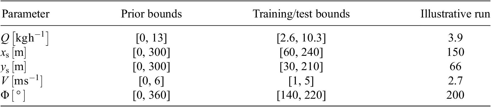

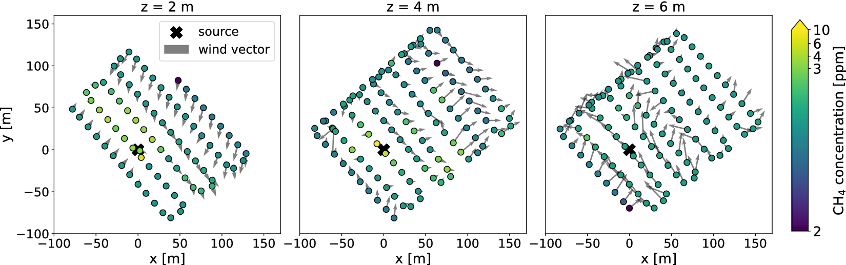


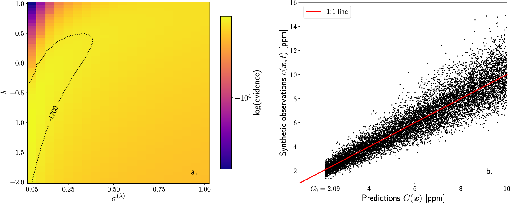


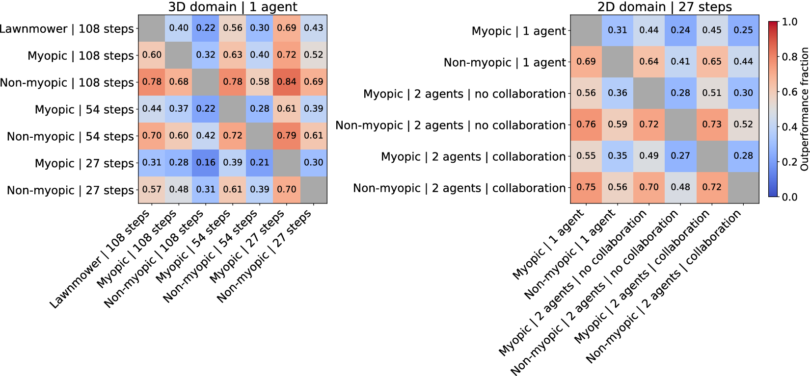


 Open access
Comments
Dear editors,
We are pleased to submit our manuscript ‘Actively inferring methane sources with drones’ for consideration in the special edition of Environmental Data Science on ‘Connecting Data-Driven and Physical Approaches: Application to Climate Modeling and Earth System Observation’.
In this study, we present a framework that integrates Bayesian inference with deep reinforcement learning (RL) to guide drone-based sampling for methane source estimation in unfamiliar environments. Using a calibrated observation model derived from real-world drone measurements, we demonstrate that non-myopic (far-sighted) navigation strategies trained via RL consistently outperform both myopic (short-sighted) and preplanned lawnmower strategies in terms of precision and accuracy of estimated source location and emission rate.
Our findings advance intelligent, data-driven sampling strategies for environmental monitoring, with potential applications in climate science, emissions reporting, and regulatory compliance.
We appreciate your consideration and look forward to your response.
Kind regards,
Alouette van Hove
Kristoffer Aalstad
Norbert Pirk