


1. Introduction
Many air vehicles operate in highly unsteady aerodynamic environments, such as gust encounters (Jones, Cetiner & Smith Reference Jones, Cetiner and Smith2022). Estimating transient flow fields and aerodynamic loads from sparse measurements in such scenarios is a complex inverse problem due to disturbed flow fields. Accurate flow and aerodynamic load prediction is critical for aerodynamic control, as it enables the design of robust control systems and adaptive mechanisms for dynamic flow conditions. By accurately reconstructing flow fields and quantifying uncertainties, these estimations enhance sensor-based predictions in gust-encounter scenarios, improving the overall reliability of aerodynamic performance. Traditional Bayesian approaches, such as the ensemble Kalman filter and its variants, have been widely used to incorporate uncertainty into predictions (Le Provost & Eldredge Reference Le Provost and Eldredge2021; Le Provost et al. Reference Le Provost, Baptista, Marzouk and Eldredge2022), but their performance can be limited in high-dimensional state spaces due to sampling errors and the need for large ensemble sizes. This highlights the need for more robust, data-driven techniques for modelling input–output relationships that can be utilised offline for efficient predictions. Deep learning (DL), known for its ability to learn complex and nonlinear mappings, offers a promising alternative. For instance, Dubois et al. (Reference Dubois, Gomez, Planckaert and Perret2022) utilised both linear and nonlinear neural networks (NNs) to reconstruct velocity fields, while Zhong et al. (Reference Zhong, Fukami, An and Taira2023) developed a model using long–short term memory and transfer learning for aerodynamic force and wake reconstruction. Chen et al. (Reference Chen, Kaiser, Hu, Rival, Fukami and Taira2024) applied a multi-layer perceptron (MLP) to estimate aerodynamic loads from surface pressure measurements. Despite these advances, challenges remain in managing numerous parameters and mitigating computational costs for high-dimensional data.
Modern DL constitutes an incredibly powerful tool for regression and classification tasks, as well as for reinforcement learning, where an agent interacts with the environment and learns to take actions that maximise rewards. Deep learning has garnered tremendous attention from researchers across various fields, including physics, biology, medicine and engineering (Ching et al. Reference Ching2018; Akay & Hess Reference Akay and Hess2019; Tanaka, Tomiya & Hashimoto Reference Tanaka, Tomiya and Hashimoto2021; Che et al. Reference Che, Liu, Li, Huang and Hu2023). Despite their broad applicability, DL models are prone to overfitting (Brunton & Kutz Reference Brunton and Kutz2022). Moreover, they tend to be overconfident in their predictions, which is particularly problematic in decision-making applications such as safety-critical systems (Le et al. Reference Le, Diehl, Brunner and Knoll2018), medical diagnosis (Laves et al. Reference Laves, Ihler, Ortmaier and Kahrs2019) and autonomous driving (Shafaei et al. Reference Shafaei, Kugele, Osman and Knoll2018). Overconfident predictions can lead to poor decision making and potentially catastrophic consequences if the model’s predictions are trusted without question. Therefore, it is crucial to train uncertainty-aware NNs to mitigate these risks and ensure reliable predictions.
There are generally two main sources of uncertainty in DL, i.e. aleatoric and epistemic uncertainties (Hüllermeier & Waegeman Reference Hüllermeier and Waegeman2021). Aleatoric uncertainty – also known as data uncertainty – refers to the irreducible uncertainty in data that gives rise to uncertainty in predictions. This type of uncertainty is due to the randomness and noise inherent in the measurements or observations. Aleatoric uncertainty is intrinsic to the process being studied and cannot be eliminated. In contrast, epistemic uncertainty – also known as model uncertainty – arises from the lack of knowledge about the best model to describe the underlying data-generating process. To better illustrate epistemic uncertainty, we consider two common cases of poorly fitted models in DL: underfitting and overfitting. In both scenarios, the model exhibits high epistemic uncertainty when making predictions on unseen data. Unlike aleatoric uncertainty, this type of uncertainty can be reduced by gathering more data or improving the model. Various approaches exist to propagate data uncertainty through artificial neural networks. One prevalent method is moment matching (Frey & Hinton Reference Frey and Hinton1999; Petersen et al. Reference Petersen, Mishra, Kuehne, Borgelt, Deussen and Yurochkin2024), which involves propagating the first two moments of a distribution through the network. However, this method increases the number of learned parameters in the network and adds computational cost, especially for large networks. Researchers have also utilised variational autoencoders to extract a stochastic latent space from noisy data (Gundersen et al. Reference Gundersen, Oleynik, Blaser and Alendal2021; Liu, Grana & de Reference Liu, Grana and de Figueiredo2022).
Bayesian probability theory offers a robust framework for addressing model uncertainty. In particular, Bayesian neural networks (BNNs), thoroughly reviewed in Jospin et al. (Reference Jospin, Laga, Boussaid, Buntine and Bennamoun2022), are stochastic NNs trained using Bayesian inference. The BNNs can model both aleatoric and epistemic uncertainties. Aleatoric uncertainty is addressed by learning the parameters of a probability distribution at the last layer that approximates the true distribution (Jospin et al. Reference Jospin, Laga, Boussaid, Buntine and Bennamoun2022). Epistemic uncertainty, on the other hand, is modelled by introducing stochastic weights or activations in the DL models. By specifying a prior distribution over these stochastic parameters and defining a likelihood function, the exact posterior distribution can be learned through Bayes’ rule using Markov chain Monte Carlo (MCMC) (Salakhutdinov & Mnih Reference Salakhutdinov and Mnih2008) or approximated with a family of distributions using variational inference (VI) (Swiatkowski et al. Reference Swiatkowski2020).
In spite of their clear advantages for modelling uncertainty, BNNs often come with prohibitive computational costs and are challenging to converge for large models. However, we can draw upon key aspects of BNN structure, e.g. learning parameters of a model distribution, to capture aleatoric uncertainty in an efficient manner. Moreover, Gal & Ghahramani (Reference Gal and Ghahramani2016a ,Reference Gal and Ghahramani b ) have proved that we can interpret dropout in a NN – which is traditionally used to prevent overfitting (Srivastava et al. Reference Srivastava, Hinton, Krizhevsky, Sutskever and Salakhutdinov2014) – as a Bayesian approximation of a Gaussian process (Williams & Rasmussen Reference Williams and Rasmussen2006), without modifying the models themselves. Monte Carlo dropout, known as MC dropout, can be used to estimate the uncertainty of the model (Gal & Ghahramani Reference Gal and Ghahramani2016b ). In another study, Kendall & Gal (Reference Kendall and Gal2017) successfully integrated both aleatoric and epistemic uncertainties into a single computer vision model.
This paper aims to estimate aerodynamic flow fields and load from sensor measurements while incorporating uncertainty quantification within DL models. In particular, we use machine learning tools to reconstruct the flow field and the lift coefficient under extreme aerodynamic conditions from sparse surface pressure measurements. Our approach leverages a nonlinear lift-augmented autoencoder, as proposed by Fukami & Taira (Reference Fukami and Taira2023), which captures low-dimensional representations of the complex flow dynamics, for improved sensor-based estimation. In this framework, we rigorously analyse the sensor response to gust–airfoil interactions, providing insight into optimal sensor placement. To further enhance prediction robustness, we introduce novel approaches for modelling uncertainties in DL predictions, distinguishing between epistemic (model) and aleatoric (data) uncertainties. Following the methodology of Gal & Ghahramani (Reference Gal and Ghahramani2016a ,Reference Gal and Ghahramani b ), we apply MC dropout to treat the network stochastically and capture model uncertainty. To capture data uncertainty, our network is trained to estimate the statistical parameters (moments) of a model distribution in a reduced-order latent space, accounting for the inherent noise in the surface pressure data. Our results demonstrate the efficacy of these methods in quantifying two types of uncertainty in a challenging aerodynamic environment.
The paper is structured as follows: § 2 outlines the problem and details the mathematical approach employed for data compression and uncertainty quantification. Section 3 presents the findings of the study. Finally, § 4 summarises the key outcomes and implications of the research.
2. Problem statement and methodology
The present study proposes a framework designed to model the intricate and uncertain relationship between input surface pressure measurements and the resulting aerodynamic forces and vortical structure. Our approach leverages advanced data compression techniques and uncertainty quantification to enhance prediction accuracy and reliability. Specifically, we employ DL models to map input surface measurements to a low-dimensional latent space, facilitating efficient reconstruction of flow fields. The framework leverages MC dropout to model epistemic uncertainty in the NN, while incorporating learned loss attenuation to address how measurement noise affects predictions. This combined approach enables robust quantification of confidence intervals, providing a comprehensive assessment of uncertainty in the predictions.
This section outlines the mathematical framework of our approach, covering the problem formulation, NN architecture and model training and validation using high-fidelity simulation data. Additionally, we discuss the construction of the latent space and the integration of uncertainty quantification techniques into the predictive model, ensuring accurate and reliable performance.
2.1. Problem statement
Given sparse pressure measurements from surface sensors, the goal of this work is to estimate the vorticity field and aerodynamic loads from a probabilistic perspective. For data generation in this study, we consider unsteady two-dimensional flow over a NACA 0012 airfoil positioned at a range of angles of attack $\alpha \in \{20^\circ , 30^\circ ,$ $40^\circ , 50^\circ , 60^\circ \}$
. The free-stream velocity is denoted by
$40^\circ , 50^\circ , 60^\circ \}$
. The free-stream velocity is denoted by $U_{\infty }$
with the chord-based Reynolds number
$U_{\infty }$
with the chord-based Reynolds number $Re=U_\infty c/\nu =100$
, where
$Re=U_\infty c/\nu =100$
, where $c$
is the chord length and
$c$
is the chord length and $\nu$
is the fluid kinematic viscosity. The case at
$\nu$
is the fluid kinematic viscosity. The case at $\alpha = 20^\circ$
corresponds to a nearly steady flow, while vortex shedding is observed at higher angles of attack. For gust-encounter aerodynamics, the disturbance vortex is modelled as a Taylor vortex (Taylor Reference Taylor1918)
$\alpha = 20^\circ$
corresponds to a nearly steady flow, while vortex shedding is observed at higher angles of attack. For gust-encounter aerodynamics, the disturbance vortex is modelled as a Taylor vortex (Taylor Reference Taylor1918)
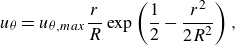 \begin{equation} u_\theta = u_{\theta ,max} \frac {r}{R} \exp \left ( \frac {1}{2} - \frac {r^2}{2R^2} \right ), \end{equation}
where $R$
is the radius and
$R$
is the radius and $u_{\theta ,max}$
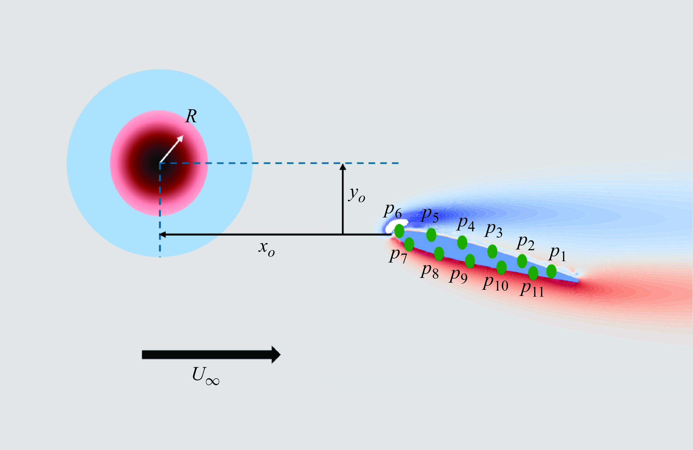
is the maximum rotational velocity of the vortex. The problem configuration, including the position of sensors and their indices, is illustrated in figure 1. The vortex is initially placed upstream of the airfoil at
$u_{\theta ,max}$
is the maximum rotational velocity of the vortex. The problem configuration, including the position of sensors and their indices, is illustrated in figure 1. The vortex is initially placed upstream of the airfoil at $(x_o,y_o)$
with
$(x_o,y_o)$
with $x_o/c=-2$
, with the origin
$x_o/c=-2$
, with the origin $(0,0)$
set at the tip of the airfoil. The vortex strength is characterised by
$(0,0)$
set at the tip of the airfoil. The vortex strength is characterised by $G \equiv u_{\theta ,max}/U_{\infty }$
. We consider cases with randomly sampled parameters:
$G \equiv u_{\theta ,max}/U_{\infty }$
. We consider cases with randomly sampled parameters: $G \in [-1,1]$
,
$G \in [-1,1]$
, $y_o/c \in [-0.5,0.5]$
and
$y_o/c \in [-0.5,0.5]$
and $2R/c \in [0.5,1]$
. The direct numerical simulation of the Navier–Stokes equations in vorticity–streamfunction form is carried out by using the lattice Green’s function/immersed layers method proposed by Eldredge (Reference Eldredge2022) over a domain size of
$2R/c \in [0.5,1]$
. The direct numerical simulation of the Navier–Stokes equations in vorticity–streamfunction form is carried out by using the lattice Green’s function/immersed layers method proposed by Eldredge (Reference Eldredge2022) over a domain size of $(-4c,4c) \times (-2c,2c)$
on a Cartesian grid with uniform spacing
$(-4c,4c) \times (-2c,2c)$
on a Cartesian grid with uniform spacing $\Delta x/c = 0.02$
. (The use of the lattice Green’s function enables a much tighter domain than other conventional flow techniques.) We numerically calculate the surface pressure
$\Delta x/c = 0.02$
. (The use of the lattice Green’s function enables a much tighter domain than other conventional flow techniques.) We numerically calculate the surface pressure $p_s$
relative to ambient pressure
$p_s$
relative to ambient pressure $p_\infty$
, and define the pressure coefficient for discussion purposes as follows:
$p_\infty$
, and define the pressure coefficient for discussion purposes as follows:
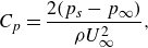 \begin{equation} C_p = \frac {2(p_s - p_\infty )}{\rho U_\infty ^2}, \end{equation}
where $\rho$
represents the fluid density.
$\rho$
represents the fluid density.
Configuration of the problem, illustrating the relative position of the gust centre with respect to the airfoil tip, the size of the disturbance and the indices of sensors mounted on the airfoil.
Data for the regression task are collected from a portion of the computational domain, specifically $(-0.9c,3.9c) \times (-1.2c,1.2c)$
. This region is chosen to balance computational efficiency with accuracy, ensuring that the gust is fully captured throughout its interaction with the airfoil and wake. For each angle of attack, one base (undisturbed) case and a total of 20 gust cases are considered, generating a dataset with 5 base cases and 100 gust cases. Each case is simulated over a non-dimensional duration of 15 convective time units, defined as
$(-0.9c,3.9c) \times (-1.2c,1.2c)$
. This region is chosen to balance computational efficiency with accuracy, ensuring that the gust is fully captured throughout its interaction with the airfoil and wake. For each angle of attack, one base (undisturbed) case and a total of 20 gust cases are considered, generating a dataset with 5 base cases and 100 gust cases. Each case is simulated over a non-dimensional duration of 15 convective time units, defined as $t \equiv t^{\prime } U_\infty /c$
with
$t \equiv t^{\prime } U_\infty /c$
with $t^{\prime }$
being the dimensional time, from the instant the disturbance is introduced to the flow. A total of 745 snapshots are uniformly sampled over time for each case, yielding 78 225 data points across the full dataset. This temporal resolution has been verified to be sufficient to capture the evolution of local flow dynamics during gust encounters.
$t^{\prime }$
being the dimensional time, from the instant the disturbance is introduced to the flow. A total of 745 snapshots are uniformly sampled over time for each case, yielding 78 225 data points across the full dataset. This temporal resolution has been verified to be sufficient to capture the evolution of local flow dynamics during gust encounters.
2.2. Low-order representation of flow
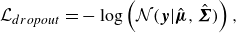
Training a model to map sparse, low-dimensional measurements to a high-dimensional flow field necessitates deep architectures with numerous layers and nodes, which can lead to computational intractability. This challenge is particularly pronounced in the context of uncertainty quantification, as the cross-correlations within the high-dimensional output significantly increase the data size, complicating training and computational efficiency. Building on the findings of Fukami & Taira (Reference Fukami and Taira2023), we utilise a nonlinear lift-augmented autoencoder to derive a low-dimensional representation of the high-dimensional gust-encounter flow field. Before tackling uncertainty quantification, we first focus on data-driven flow compression to identify this low-dimensional space, which effectively captures the key physics of vortex–gust–airfoil interactions. We adopt the network architecture described in Fukami & Taira (Reference Fukami and Taira2023), which integrates a MLP with a convolutional NN. As illustrated in figure 2, (a), our data compression framework comprises an encoder $\mathcal{F}_e$
that reduces the high-dimensional data into a low-dimensional latent vector
$\mathcal{F}_e$
that reduces the high-dimensional data into a low-dimensional latent vector $\boldsymbol{\xi } \in \mathbb{R}^l$
, where
$\boldsymbol{\xi } \in \mathbb{R}^l$
, where $l\ll n$
, with
$l\ll n$
, with $n$
the data dimension. In our applications in this paper,
$n$
the data dimension. In our applications in this paper, $l=3$
, as in Fukami & Taira (Reference Fukami and Taira2023); the appropriateness of this choice is further supported by empirical observations: increasing
$l=3$
, as in Fukami & Taira (Reference Fukami and Taira2023); the appropriateness of this choice is further supported by empirical observations: increasing $l$
beyond 3 does not yield a significant reduction in reconstruction loss. The encoder is followed by two decoders
$l$
beyond 3 does not yield a significant reduction in reconstruction loss. The encoder is followed by two decoders $\mathcal{F}_d$
: one for reconstructing the vorticity field
$\mathcal{F}_d$
: one for reconstructing the vorticity field $\boldsymbol{\omega }$
and another for estimating the lift coefficient
$\boldsymbol{\omega }$
and another for estimating the lift coefficient $C_L$
.
$C_L$
.
Overview of the network architecture in the present study. The flow field data are compressed into a three-dimensional latent vector, denoted as $\boldsymbol{\xi }$
, using the lift-augmented autoencoder. The architecture of this autoencoder is shown in (a). In the subsequent step, a pressure-based (MLP) network is trained to estimate the statistical parameters of a model distribution in the latent space, as illustrated on the left side of (b). This estimated latent vector sampled from the model distribution is then input into the decoder component of the autoencoder (a) to reconstruct both the vorticity field and the lift coefficient, as depicted on the right side of (b). The outputs of the pressure map are the mean
$\boldsymbol{\xi }$
, using the lift-augmented autoencoder. The architecture of this autoencoder is shown in (a). In the subsequent step, a pressure-based (MLP) network is trained to estimate the statistical parameters of a model distribution in the latent space, as illustrated on the left side of (b). This estimated latent vector sampled from the model distribution is then input into the decoder component of the autoencoder (a) to reconstruct both the vorticity field and the lift coefficient, as depicted on the right side of (b). The outputs of the pressure map are the mean $\pmb{\mu}$
and covariance matrix
$\pmb{\mu}$
and covariance matrix $\pmb{\Sigma}$
in the latent space.
$\pmb{\Sigma}$
in the latent space.
The weights are determined by solving an optimisation problem that involves minimising the loss function, defined as
 \begin{equation} \unicode{x1D652} = \text{argmin}_{\unicode{x1D652}} \left ( ||\boldsymbol{\omega } - \hat {\boldsymbol{\omega }}||_2 + \beta ||C_L - \hat {C}_L||_2 \right ), \end{equation}
where the hat over the parameters denotes the predicted field using the NN. Here, $\beta$
is a coefficient that balances the losses associated with vorticity and lift, with its value set to
$\beta$
is a coefficient that balances the losses associated with vorticity and lift, with its value set to $0.05$
, as specified in Fukami & Taira (Reference Fukami and Taira2023). The weights are optimised using the Adam optimiser. The nonlinear activation function employed is the hyperbolic tangent function.
$0.05$
, as specified in Fukami & Taira (Reference Fukami and Taira2023). The weights are optimised using the Adam optimiser. The nonlinear activation function employed is the hyperbolic tangent function.
Eighty per cent of the data are allocated for training, while the remaining 20 % are used for validation and testing. The training process utilises Early Stopping, as implemented in the TensorFlow library, to halt training if the validation loss does not improve for 200 consecutive epochs.
2.3. Flow reconstruction from sparse sensors
The reduced-order latent vector extracted in the previous section is critical for effectively capturing the vorticity field and lift. This latent vector serves as a compact, informative representation of the complex, high-dimensional flow dynamics, enabling efficient analysis and prediction while still preserving the essential features of the flow dynamics in the network weights. Thus, we wish to learn how observable data can be used to estimate the latent state of the flow. As illustrated in figure 2(b) on left side, we map surface pressure measurements to the latent space using a NN with MLP hidden layers, denoted by $\mathcal{F}_p$
. By leveraging the significant reduced dimensionality as the latent space representation, we can uniquely estimate the flow field and lift coefficient from available sensor data.
$\mathcal{F}_p$
. By leveraging the significant reduced dimensionality as the latent space representation, we can uniquely estimate the flow field and lift coefficient from available sensor data.
An overview of the network architecture for estimation purposes is shown in figure 2(b). The following sections will demonstrate that capturing heteroscedastic uncertainty – characterised by noise-dependent variability – requires the model to output the statistics of the low-order flow in the latent space, rather than simply providing a pointwise prediction of the latent states. In this study, we predict the mean and covariance matrix as the first two moments of a multivariate normal distribution in the latent space. To ensure that flow estimation is invariant to the absolute position of the airfoil within the computational domain, and to generalise the framework to potential different sensor configurations in future studies, we augment the readings with the $x$
and
$x$
and $y$
coordinates of each sensor, expressed in a reference frame fixed to the airfoil with its origin located at the mid-chord. These coordinates are stacked alongside the pressure measurements and the encoded angle of attack, collectively forming the input vector
$y$
coordinates of each sensor, expressed in a reference frame fixed to the airfoil with its origin located at the mid-chord. These coordinates are stacked alongside the pressure measurements and the encoded angle of attack, collectively forming the input vector $\boldsymbol{p}_{stacked}$
. Including the angle of attack provides the network with critical information about the flow incidence direction, enabling it to distinguish between flow regimes associated with different orientations. Although sensor locations are fixed in our current dataset, this input structure facilitates generalisation to configurations with different sensor placements or airfoil geometries. As a result, incorporating sensor positions improves the model’s capacity to generalise beyond the specific scenarios encountered during training. In this study, 11 pressure measurements are utilised, resulting in an input vector of size 38 for the pressure-based estimator (the
$\boldsymbol{p}_{stacked}$
. Including the angle of attack provides the network with critical information about the flow incidence direction, enabling it to distinguish between flow regimes associated with different orientations. Although sensor locations are fixed in our current dataset, this input structure facilitates generalisation to configurations with different sensor placements or airfoil geometries. As a result, incorporating sensor positions improves the model’s capacity to generalise beyond the specific scenarios encountered during training. In this study, 11 pressure measurements are utilised, resulting in an input vector of size 38 for the pressure-based estimator (the $x$
and
$x$
and $y$
sensor coordinates along with the readings themselves, as well as the encoded angles of attack in the form of one of 5 cases). Weight regularisation is employed to constrain the magnitude of the network’s weights, preventing them from becoming excessively large. This helps control the model’s uncertainty, ensuring more stable and reliable predictions.
$y$
sensor coordinates along with the readings themselves, as well as the encoded angles of attack in the form of one of 5 cases). Weight regularisation is employed to constrain the magnitude of the network’s weights, preventing them from becoming excessively large. This helps control the model’s uncertainty, ensuring more stable and reliable predictions.
Once the stacked pressure measurements and sensor positions are mapped to the latent space, the pre-trained decoder component of the NN, denoted by $\mathcal{F}_d$
, from the lift-augmented autoencoder as detailed in § 2.2, can be adopted to reconstruct the vorticity field and lift from this latent vector. This reconstruction process, depicted in figure 2(b) on the right side, leverages the network’s ability to translate the reduced-order representation back into the high-dimensional physical space with high fidelity. The advantage of this general approach is its capability to reconstruct the flow field and lift from limited measurements without sacrificing generality or requiring a large network. By focusing on the latent vector, we ensure that the essential characteristics of the flow are captured, enabling accurate predictions even with sparse data. Both the autoencoder and inference networks are trained on a dataset encompassing both undisturbed and strongly disturbed cases.
$\mathcal{F}_d$
, from the lift-augmented autoencoder as detailed in § 2.2, can be adopted to reconstruct the vorticity field and lift from this latent vector. This reconstruction process, depicted in figure 2(b) on the right side, leverages the network’s ability to translate the reduced-order representation back into the high-dimensional physical space with high fidelity. The advantage of this general approach is its capability to reconstruct the flow field and lift from limited measurements without sacrificing generality or requiring a large network. By focusing on the latent vector, we ensure that the essential characteristics of the flow are captured, enabling accurate predictions even with sparse data. Both the autoencoder and inference networks are trained on a dataset encompassing both undisturbed and strongly disturbed cases.
2.4. Informative directions of measurements
Not all measurements contribute equally to estimating the flow field at each time step. The most responsive measurement subspace contains the most informative directions for capturing the flow field’s dynamics. These directions reflect how the estimated flow field is most sensitive to particular weighted combinations of sensor measurements. This subspace evolves due to the transient nature of vortex shedding behind the airfoil and gust–airfoil interactions.
In this section, we outline the methodology for analysing the sensitivity of our NN model, which maps inputs $\boldsymbol{x}$
to outputs
$\boldsymbol{x}$
to outputs $\boldsymbol{y}$
through a nonlinear function
$\boldsymbol{y}$
through a nonlinear function $\boldsymbol{y}=\boldsymbol{f}(\boldsymbol{x};\unicode{x1D652}\kern2pt)$
, where
$\boldsymbol{y}=\boldsymbol{f}(\boldsymbol{x};\unicode{x1D652}\kern2pt)$
, where $\unicode{x1D652}$
represents the network parameters, including weights and biases in a typical deep network. In this study, inputs
$\unicode{x1D652}$
represents the network parameters, including weights and biases in a typical deep network. In this study, inputs $\boldsymbol{x} \in \mathbb{R}^d$
correspond to the measurements augmented with the sensor coordinates, denoted by
$\boldsymbol{x} \in \mathbb{R}^d$
correspond to the measurements augmented with the sensor coordinates, denoted by $\boldsymbol{p}_{stacked}$
, while the output
$\boldsymbol{p}_{stacked}$
, while the output $\boldsymbol{y} \in \mathbb{R}^l$
of the NN is the
$\boldsymbol{y} \in \mathbb{R}^l$
of the NN is the $l$
-dimensional latent vector
$l$
-dimensional latent vector $\boldsymbol{\xi }$
. The nonlinear mapping from inputs to outputs
$\boldsymbol{\xi }$
. The nonlinear mapping from inputs to outputs $\boldsymbol{f} : \mathbb{R}^d \rightarrow \mathbb{R}^l$
in this context refers to
$\boldsymbol{f} : \mathbb{R}^d \rightarrow \mathbb{R}^l$
in this context refers to $\mathcal{F}^d_p$
which is similar to
$\mathcal{F}^d_p$
which is similar to $\mathcal{F}_p$
in the previous section, but with the output restricted to the mean prediction, i.e. we assume a deterministic form of the NN for this discussion. Additionally, to neglect the effect of model uncertainty in this section, the dropout layers in the
$\mathcal{F}_p$
in the previous section, but with the output restricted to the mean prediction, i.e. we assume a deterministic form of the NN for this discussion. Additionally, to neglect the effect of model uncertainty in this section, the dropout layers in the $\mathcal{F}^d_p$
are active only during training. For clarity and consistency, we use
$\mathcal{F}^d_p$
are active only during training. For clarity and consistency, we use $\boldsymbol{x}$
,
$\boldsymbol{x}$
, $\boldsymbol{y}$
and
$\boldsymbol{y}$
and $\boldsymbol{f}$
in general form to refer to inputs, outputs and the mapping between them, respectively, in the derivations presented in this section.
$\boldsymbol{f}$
in general form to refer to inputs, outputs and the mapping between them, respectively, in the derivations presented in this section.
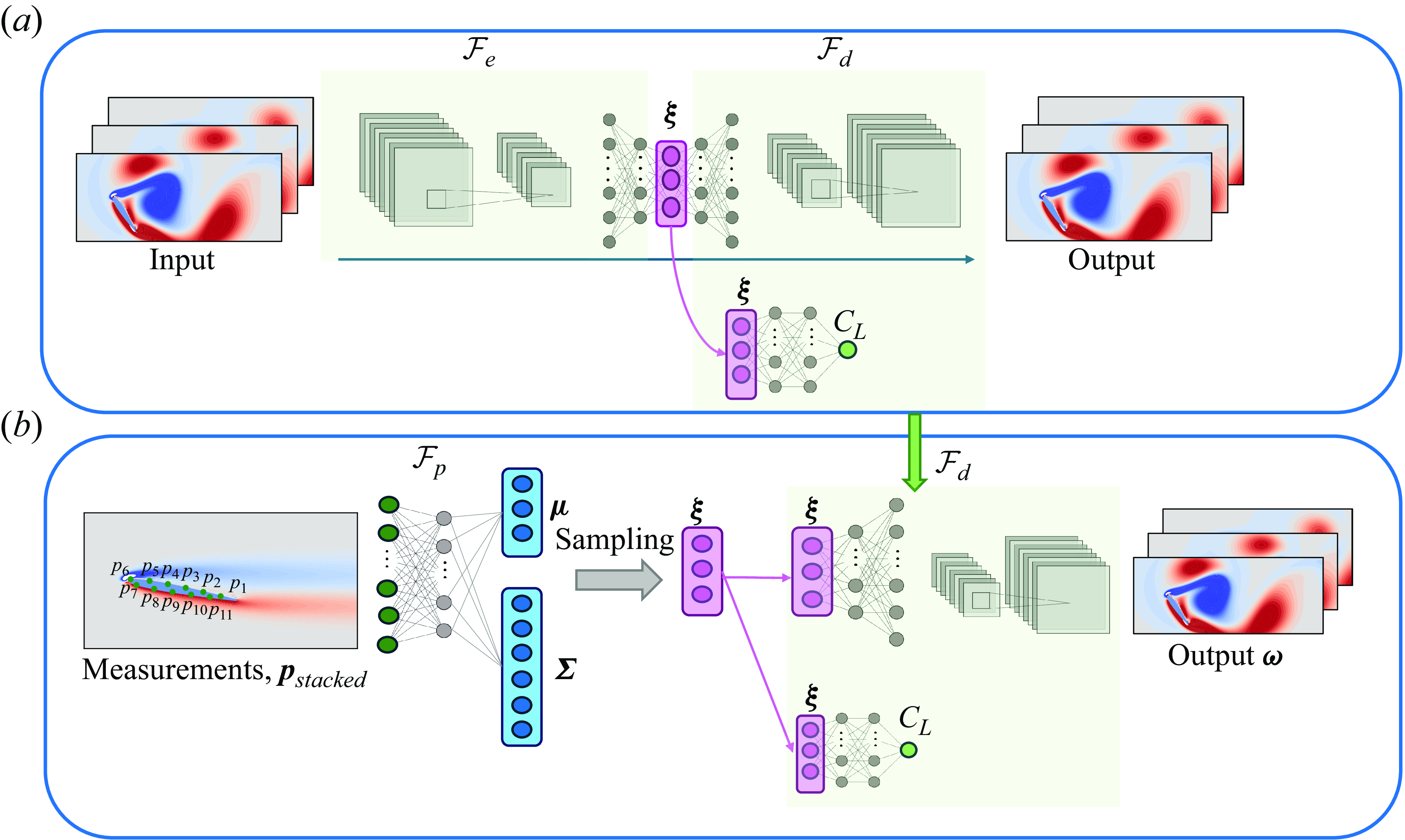
For stochastic inputs and outputs influenced by sensor noise, the primary directions in the measurement space in which measurements are most informative of variations in the flow field (via the latent space) can be identified using the Gramian matrix of the Jacobian in the input space, defined as follows (Quinton & Rey Reference Quinton and Rey2024):
 \begin{equation} \unicode{x1D63E}_{\unicode{x1D66D}} = \mathbb{E} [\nabla \boldsymbol{f}(\boldsymbol{x})^T \ \nabla \boldsymbol{f}(\boldsymbol{x})], \end{equation}
where $\mathbb{E}[\cdot ]$
denotes the expectation with respect to the noisy input
$\mathbb{E}[\cdot ]$
denotes the expectation with respect to the noisy input $\boldsymbol{x}$
, and
$\boldsymbol{x}$
, and $\nabla \boldsymbol{f}$
represents the Jacobian matrix that describes the derivatives of the output vector
$\nabla \boldsymbol{f}$
represents the Jacobian matrix that describes the derivatives of the output vector $\boldsymbol{y}$
with respect to the input vector
$\boldsymbol{y}$
with respect to the input vector $\boldsymbol{x}$
. We call
$\boldsymbol{x}$
. We call
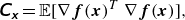
 $\unicode{x1D63E}_{\unicode{x1D66D}}$
the measurement space Gramian, and revisit (2.4) to obtain
$\unicode{x1D63E}_{\unicode{x1D66D}}$
the measurement space Gramian, and revisit (2.4) to obtain
 \begin{equation} \unicode{x1D63E}_{\unicode{x1D66D}} = \int \nabla \boldsymbol{f}(\boldsymbol{x})^T \ \nabla \boldsymbol{f}(\boldsymbol{x}) {\rm d}\pi (\boldsymbol{x}), \end{equation}
where $\pi (\boldsymbol{x})$
is the probability density function of the input
$\pi (\boldsymbol{x})$
is the probability density function of the input $\boldsymbol{x}$
. The matrix
$\boldsymbol{x}$
. The matrix $\unicode{x1D63E}_{\unicode{x1D66D}}$
is positive semi-definite, and its eigendecomposition can be written as
$\unicode{x1D63E}_{\unicode{x1D66D}}$
is positive semi-definite, and its eigendecomposition can be written as $\unicode{x1D63E}_{\unicode{x1D66D}} = \boldsymbol{U} \boldsymbol{\Lambda }_x^2 \boldsymbol{U}^T$
, where
$\unicode{x1D63E}_{\unicode{x1D66D}} = \boldsymbol{U} \boldsymbol{\Lambda }_x^2 \boldsymbol{U}^T$
, where $\boldsymbol{U} \in \mathbb{R}^{d \times d}$
contains the eigenvectors with
$\boldsymbol{U} \in \mathbb{R}^{d \times d}$
contains the eigenvectors with $\boldsymbol{\Lambda }_x^2$
the associated eigenvalues. The eigenvectors of the measurement space Gramian identify the subspace spanned by the dominant (i.e. most informative) directions of the measurements. For convenience, we assume that the eigenvalues
$\boldsymbol{\Lambda }_x^2$
the associated eigenvalues. The eigenvectors of the measurement space Gramian identify the subspace spanned by the dominant (i.e. most informative) directions of the measurements. For convenience, we assume that the eigenvalues $\boldsymbol{\Lambda }_x^2$
are in decreasing order. In practice, we approximate these integrals using the Monte Carlo method to compute
$\boldsymbol{\Lambda }_x^2$
are in decreasing order. In practice, we approximate these integrals using the Monte Carlo method to compute $\unicode{x1D63E}_{\unicode{x1D66D}}$
. The calculations of Jacobians
$\unicode{x1D63E}_{\unicode{x1D66D}}$
. The calculations of Jacobians $\nabla \boldsymbol{f} \in \mathbb{R}^{l \times d}$
for a deterministic NN denoted here by
$\nabla \boldsymbol{f} \in \mathbb{R}^{l \times d}$
for a deterministic NN denoted here by $\mathcal{F}^d_p$
can be performed using automatic differentiation.
$\mathcal{F}^d_p$
can be performed using automatic differentiation.
For the low-order representations, only the first $r_x \leqslant d$
eigenmodes of the measurement space are retained, which correspond to dominant modes
$r_x \leqslant d$
eigenmodes of the measurement space are retained, which correspond to dominant modes $\boldsymbol{U}_r$
. The rank
$\boldsymbol{U}_r$
. The rank $r_x$
is tuned based on the decay of
$r_x$
is tuned based on the decay of $\boldsymbol{\Lambda }_x^2$
. Typically these ranks are set to achieve a threshold
$\boldsymbol{\Lambda }_x^2$
. Typically these ranks are set to achieve a threshold $\gamma \in [0,1]$
for the cumulative normalised energy of the eigenvalue spectra. The first
$\gamma \in [0,1]$
for the cumulative normalised energy of the eigenvalue spectra. The first $r_x$
eigenmodes of
$r_x$
eigenmodes of $\unicode{x1D63E}_{\unicode{x1D66D}}$
correspond to the directions in the input space that most influence the prediction of the latent space. The components of an eigenmode represent the weights on the sensors’ contributions to this mode; a larger magnitude component indicates a greater relative role for that sensor in detecting a disturbance.
$\unicode{x1D63E}_{\unicode{x1D66D}}$
correspond to the directions in the input space that most influence the prediction of the latent space. The components of an eigenmode represent the weights on the sensors’ contributions to this mode; a larger magnitude component indicates a greater relative role for that sensor in detecting a disturbance.
2.5. Quantifying aleatoric and epistemic uncertainties
In real-world applications, measurement noise is a common occurrence, and the pressure measurements in this study are no exception. This introduces uncertainty into the predictions, which is particularly critical for risk management applications where accurate quantification of uncertainty is essential. To assess the uncertainty in the outputs due to measurement noise, we define the conditional output distribution given the input and the network parameters $\unicode{x1D652}$
as
$\unicode{x1D652}$
as $\pi _a(\boldsymbol{y}|\boldsymbol{x}, \unicode{x1D652}\kern2pt)$
, where the subscript
$\pi _a(\boldsymbol{y}|\boldsymbol{x}, \unicode{x1D652}\kern2pt)$
, where the subscript $a$
denotes aleatoric uncertainty. Here, the noisy inputs are represented as
$a$
denotes aleatoric uncertainty. Here, the noisy inputs are represented as $\boldsymbol{x}=\bar {\boldsymbol{x}}+\boldsymbol{\eta }$
, with
$\boldsymbol{x}=\bar {\boldsymbol{x}}+\boldsymbol{\eta }$
, with $\bar {\boldsymbol{x}}$
referring to clean data and
$\bar {\boldsymbol{x}}$
referring to clean data and $\boldsymbol{\eta }$
representing the white sensor noise in the dominant directions of measurement space. This noise will be defined later in § 2.
$\boldsymbol{\eta }$
representing the white sensor noise in the dominant directions of measurement space. This noise will be defined later in § 2.
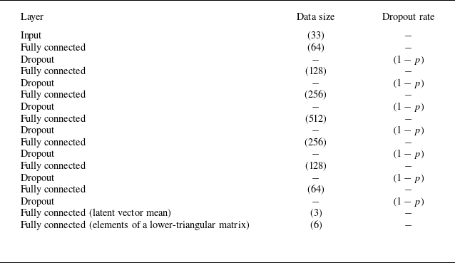
Aleatoric (or data) uncertainty, originating from inherent noise in data, must be explicitly captured to enhance the network’s resilience to noisy inputs. In real-world scenarios, the probability distribution of outputs typically varies as a function of inputs. This data-dependent nature of aleatoric uncertainty can be effectively addressed using heteroscedastic models, which incorporate learned loss attenuation to model input-dependent noise levels (Kendall & Gal Reference Kendall and Gal2017). Consequently, the network architecture depicted in figure 2 and listed in table 1 is designed specifically for uncertainty quantification. It learns the parameters of a multivariate normal distribution, i.e. the mean denoted as $\boldsymbol{\mu } \in \mathbb{R}^l$
, and the covariance matrix represented by
$\boldsymbol{\mu } \in \mathbb{R}^l$
, and the covariance matrix represented by $\boldsymbol{\Sigma } \in \mathbb{R}^{l \times l}$
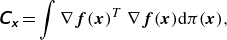
. During training, the network minimises a heteroscedastic loss function based on the negative log likelihood of a multivariate normal distribution
$\boldsymbol{\Sigma } \in \mathbb{R}^{l \times l}$
. During training, the network minimises a heteroscedastic loss function based on the negative log likelihood of a multivariate normal distribution
 \begin{equation} \mathcal{L}_{dropout} = -\log \left (\mathcal{N} (\boldsymbol{y} | \hat {\boldsymbol{\mu }} , \hat {\boldsymbol{\Sigma }}) \right ), \end{equation}
where $\boldsymbol{y}$
represents the true latent vector defined as the extracted latent vector from the autoencoder and
$\boldsymbol{y}$
represents the true latent vector defined as the extracted latent vector from the autoencoder and $\hat {\boldsymbol{\mu }}$
and
$\hat {\boldsymbol{\mu }}$
and $\hat {\boldsymbol{\Sigma }}$
are the predicted mean and covariance matrix, respectively. The multivariate normal distribution is defined as usual by
$\hat {\boldsymbol{\Sigma }}$
are the predicted mean and covariance matrix, respectively. The multivariate normal distribution is defined as usual by
Structure of the sensor-based network employed in the present study, which maps the pressure measurements to the latent variables.
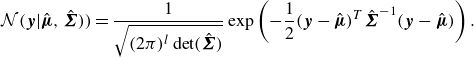 \begin{equation} \mathcal{N} (\boldsymbol{y} | \hat {\boldsymbol{\mu }} , \hat {\boldsymbol{\Sigma }})) = \frac {1}{\sqrt {(2\pi )^l \det (\hat {\boldsymbol{\Sigma }})}} \exp \left ( -\frac {1}{2} (\boldsymbol{y} - \hat {\boldsymbol{\mu }})^T \hat {\boldsymbol{\Sigma }}^{-1} (\boldsymbol{y} - \hat {\boldsymbol{\mu }}) \right ). \end{equation}
It should be noted that directly predicting a covariance matrix poses challenges since the network might not inherently ensure that the matrix is symmetric and positive definite. To address this, we reformulate the prediction: instead of predicting the full covariance matrix, the network learns $l \times (l+1)/2$
elements of a lower-triangular matrix,
$l \times (l+1)/2$
elements of a lower-triangular matrix, $\unicode{x1D647}$
, in the form of
$\unicode{x1D647}$
, in the form of
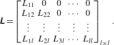 \begin{equation} \unicode{x1D647} = \begin{bmatrix} L_{11} & 0 & 0 & \cdots & 0 \\ L_{12} & L_{22} & 0 & \cdots & 0 \\ \vdots & \vdots & \vdots & \vdots & \vdots \\ L_{1l} & L_{2l} & L_{3l} & \cdots & L_{ll} \\ \end{bmatrix}_{l \times l}. \end{equation}
Considering that the dimension of the latent vector is denoted by $l$
, the predictions are in the space
$l$
, the predictions are in the space $[\hat {\boldsymbol{\mu }}, \hat {\unicode{x1D647}}] \in \mathbb{R}^{l+l(l+1)/2}$
. This guarantees uniqueness, symmetry and positive definiteness by constructing the covariance matrix as
$[\hat {\boldsymbol{\mu }}, \hat {\unicode{x1D647}}] \in \mathbb{R}^{l+l(l+1)/2}$
. This guarantees uniqueness, symmetry and positive definiteness by constructing the covariance matrix as $\boldsymbol{\Sigma } = \unicode{x1D647}\unicode{x1D647}^T$
. For numerical stability, the network predicts the logarithms of the squared diagonal elements, ensuring they remain positive, and directly outputs the off-diagonal elements. By constructing the covariance matrix this way, we ensure it remains positive definite and approximates the Cholesky decomposition. Additionally, to include uncertainty in the input measurements, we employ data augmentation during training, injecting Gaussian random noise into the inputs to simulate real-world conditions and help the model better capture aleatoric uncertainty in its predictions.
$\boldsymbol{\Sigma } = \unicode{x1D647}\unicode{x1D647}^T$
. For numerical stability, the network predicts the logarithms of the squared diagonal elements, ensuring they remain positive, and directly outputs the off-diagonal elements. By constructing the covariance matrix this way, we ensure it remains positive definite and approximates the Cholesky decomposition. Additionally, to include uncertainty in the input measurements, we employ data augmentation during training, injecting Gaussian random noise into the inputs to simulate real-world conditions and help the model better capture aleatoric uncertainty in its predictions.
Traditional DL models provide point-estimate predictions with overconfidence, and do not typically account for the uncertainty in the fitted model, called epistemic (or model) uncertainty. The main goal in model uncertainty is finding the conditional distribution over the parameters $\unicode{x1D652}$
of the NN for a given dataset of inputs
$\unicode{x1D652}$
of the NN for a given dataset of inputs $\unicode{x1D653}$
and outputs
$\unicode{x1D653}$
and outputs $\unicode{x1D654}$
, i.e.
$\unicode{x1D654}$
, i.e. $\pi (\unicode{x1D652}|\unicode{x1D653},\unicode{x1D654}\kern2pt)$
. Among the different ways to estimate uncertainty in the NN model, the Bayesian paradigm provides a powerful mathematical framework. Indeed, Bayes’ rule expresses the desired conditional distribution as a posterior distribution, starting from a prior
$\pi (\unicode{x1D652}|\unicode{x1D653},\unicode{x1D654}\kern2pt)$
. Among the different ways to estimate uncertainty in the NN model, the Bayesian paradigm provides a powerful mathematical framework. Indeed, Bayes’ rule expresses the desired conditional distribution as a posterior distribution, starting from a prior $\pi (\unicode{x1D652}\kern2pt)$
over the weights
$\pi (\unicode{x1D652}\kern2pt)$
over the weights
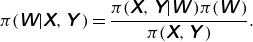 \begin{equation} \pi (\unicode{x1D652}|\unicode{x1D653},\unicode{x1D654}\kern2pt) = \frac {\pi (\unicode{x1D653},\unicode{x1D654}|\unicode{x1D652}\kern2pt) \pi (\unicode{x1D652}\kern2pt)}{\pi (\unicode{x1D653},\unicode{x1D654}\kern2pt)}. \end{equation}
Here, $\pi (\textbf{X},\textbf{Y}|\unicode{x1D652}\kern2pt)$
is the conditional probability of the data, given a particular set of weights. The denominator in this equation is the marginal distribution over the space of model parameters
$\pi (\textbf{X},\textbf{Y}|\unicode{x1D652}\kern2pt)$
is the conditional probability of the data, given a particular set of weights. The denominator in this equation is the marginal distribution over the space of model parameters $\unicode{x1D652}$
. Calculating this marginal distribution is challenging. Basically, there are two primary approaches to address this difficulty: MCMC, which samples from the true posterior and avoids the need for the denominator by only relying on comparison, and VI (Blei, Kucukelbir & McAuliffe Reference Blei, Kucukelbir and McAuliffe2017), which approximates the posterior with a known family of distributions denoted by
$\unicode{x1D652}$
. Calculating this marginal distribution is challenging. Basically, there are two primary approaches to address this difficulty: MCMC, which samples from the true posterior and avoids the need for the denominator by only relying on comparison, and VI (Blei, Kucukelbir & McAuliffe Reference Blei, Kucukelbir and McAuliffe2017), which approximates the posterior with a known family of distributions denoted by $q(\unicode{x1D652}\kern2pt)$
. The MCMC converges very slowly in large and complex networks and requires a large number of samples to achieve convergence. As an efficient alternative for obtaining the posterior distribution, deep NNs with dropout applied before every dense layer have been shown to be mathematically equivalent to approximate VI in a deep Gaussian process (Gal & Ghahramani Reference Gal and Ghahramani2016a
). This procedure, known as MC dropout, uses a variational distribution defined for each weight matrix as follows:
$q(\unicode{x1D652}\kern2pt)$
. The MCMC converges very slowly in large and complex networks and requires a large number of samples to achieve convergence. As an efficient alternative for obtaining the posterior distribution, deep NNs with dropout applied before every dense layer have been shown to be mathematically equivalent to approximate VI in a deep Gaussian process (Gal & Ghahramani Reference Gal and Ghahramani2016a
). This procedure, known as MC dropout, uses a variational distribution defined for each weight matrix as follows:
 \begin{align} z_{i,j} &\sim \text{Bernoulli} (p_i), \nonumber\\ \unicode{x1D652}_i &= \textbf{M}_i \cdot \text{diag} (\boldsymbol{z}_i), \end{align}
with $z_{i,j}$
referring to the random activation coefficient for the
$z_{i,j}$
referring to the random activation coefficient for the $j$
th neuron in the
$j$
th neuron in the $i$
th layer (1 with probability
$i$
th layer (1 with probability $p_i$
for layer
$p_i$
for layer $i$
and 0 with probability (
$i$
and 0 with probability ( $1-p_i$
)), and
$1-p_i$
)), and $\boldsymbol{z}_i$
being the random activation coefficient vector, containing all
$\boldsymbol{z}_i$
being the random activation coefficient vector, containing all $z_{i,j}$
for layer
$z_{i,j}$
for layer $i$
. The matrix
$i$
. The matrix $\textbf{M}_i$
is the matrix of weights before dropout is applied. This approximate distribution, as proven in Gal & Ghahramani (Reference Gal and Ghahramani2016a
), minimises the Kullback–Leibler divergence (
$\textbf{M}_i$
is the matrix of weights before dropout is applied. This approximate distribution, as proven in Gal & Ghahramani (Reference Gal and Ghahramani2016a
), minimises the Kullback–Leibler divergence ( $D_{KL}$
), which measures the similarity between two distributions
$D_{KL}$
), which measures the similarity between two distributions $D_{KL}(q(\unicode{x1D652}\kern2pt)||\pi (\unicode{x1D652}|\unicode{x1D653},\unicode{x1D654}\kern2pt))$
.
$D_{KL}(q(\unicode{x1D652}\kern2pt)||\pi (\unicode{x1D652}|\unicode{x1D653},\unicode{x1D654}\kern2pt))$
.
The architecture of the NN used to map surface measurements to the low-dimensional latent space $\mathcal{F}_p$
, accounting for both aleatoric and epistemic uncertainty, is detailed in table 1. In this network, to adopt MC dropout approach, dropout layers are strategically incorporated after each dense layer.
$\mathcal{F}_p$
, accounting for both aleatoric and epistemic uncertainty, is detailed in table 1. In this network, to adopt MC dropout approach, dropout layers are strategically incorporated after each dense layer.
In MC dropout, a subset of activations is randomly set to zero during training, and the same values are used in the backward pass to propagate the derivatives to the parameters. In typical NNs, dropout is usually turned off during evaluation. However, leaving it on during inference produces a distribution for the output predictions, allowing for the estimation of uncertainty in the predictions in the form of
 \begin{equation} \pi _e(\boldsymbol{y}|\boldsymbol{x},\unicode{x1D653},\unicode{x1D654}\kern2pt) = \int \pi (\boldsymbol{y}|\boldsymbol{x},\unicode{x1D652}\kern2pt) q(\unicode{x1D652}\kern2pt) {\rm d}\unicode{x1D652}. \end{equation}
The subscript $e$
in
$e$
in $\pi _e(\boldsymbol{y}|\boldsymbol{x},\unicode{x1D653},\unicode{x1D654}\kern2pt)$
denotes epistemic uncertainty. Using the Monte Carlo method, multiple stochastic forward passes are performed to approximate this integral, effectively sampling from the posterior distribution.
$\pi _e(\boldsymbol{y}|\boldsymbol{x},\unicode{x1D653},\unicode{x1D654}\kern2pt)$
denotes epistemic uncertainty. Using the Monte Carlo method, multiple stochastic forward passes are performed to approximate this integral, effectively sampling from the posterior distribution.
Although MC dropout is utilised to quantify model uncertainty, the dropout layers in the network $\mathcal{F}_p$
remain active during both training and inference, and thus affect both forms of uncertainty quantification. As described earlier, aleatoric uncertainty is quantified with a network that produces two outputs: the mean of the latent vector,
$\mathcal{F}_p$
remain active during both training and inference, and thus affect both forms of uncertainty quantification. As described earlier, aleatoric uncertainty is quantified with a network that produces two outputs: the mean of the latent vector, $\boldsymbol{\mu } \in \mathbb{R}^l$
, and the covariance matrix of the latent vector
$\boldsymbol{\mu } \in \mathbb{R}^l$
, and the covariance matrix of the latent vector $\boldsymbol{\Sigma } \in \mathbb{R}^{l\times l}$
. By applying different instances of MC dropout,
$\boldsymbol{\Sigma } \in \mathbb{R}^{l\times l}$
. By applying different instances of MC dropout, $\mathcal{F}_p$
produces a distribution of the output, and this can be assumed to be multivariate Gaussian with its statistics represented by the expected value and covariance of the output samples obtained from
$\mathcal{F}_p$
produces a distribution of the output, and this can be assumed to be multivariate Gaussian with its statistics represented by the expected value and covariance of the output samples obtained from $T$
stochastic forward passes. As such, during inference, the aleatoric predictive distribution, marginalised over the network weights, is measured by
$T$
stochastic forward passes. As such, during inference, the aleatoric predictive distribution, marginalised over the network weights, is measured by
 \begin{equation} \pi _a(\boldsymbol{y}|\boldsymbol{x},\unicode{x1D653},\unicode{x1D654}\kern2pt) = \mathcal{N} \left (\boldsymbol{y};\frac {1}{T} \sum _{k=1}^T \hat {\boldsymbol{\mu }}_k, \frac {1}{T} \sum _{k=1}^T \hat {\boldsymbol{\Sigma }}_k \right ). \end{equation}
Additionally, the epistemic predictive distribution is computed by
 \begin{equation} \pi _e(\boldsymbol{y}|\boldsymbol{x},\unicode{x1D653},\unicode{x1D654}\kern2pt) = \mathcal{N} \left (\boldsymbol{y};\frac {1}{T} \sum _{k=1}^T \hat {\boldsymbol{\mu }}_k, \text{Cov} \left ( \{\hat {\boldsymbol{\mu }}_k \}_{k=1}^T \right ) \right ), \end{equation}
with $\{ \hat {\boldsymbol{\mu }}_k, \hat {\boldsymbol{\Sigma }}_k \}_{k=1}^T$
a set of
$\{ \hat {\boldsymbol{\mu }}_k, \hat {\boldsymbol{\Sigma }}_k \}_{k=1}^T$
a set of $T$
sampled outputs. The convergence study was conducted to determine an appropriate value for
$T$
sampled outputs. The convergence study was conducted to determine an appropriate value for $T$
that ensures reliable and stable uncertainty estimates. We emphasise that the output covariance associated with the aleatoric uncertainty is predicted directly by the network and averaged over the dropout passes (the mean of the covariances), while the output covariance of the epistemic distribution follows from the spread in the pointwise predictions of the output over these passes (the covariance of the means).
$T$
that ensures reliable and stable uncertainty estimates. We emphasise that the output covariance associated with the aleatoric uncertainty is predicted directly by the network and averaged over the dropout passes (the mean of the covariances), while the output covariance of the epistemic distribution follows from the spread in the pointwise predictions of the output over these passes (the covariance of the means).
To quantify the uncertainty in the output most influenced by variations in the input during inference, we introduce noise $\boldsymbol{\eta }$
aligned with the principal directions of measurement variation. These directions are identified by the matrix
$\boldsymbol{\eta }$
aligned with the principal directions of measurement variation. These directions are identified by the matrix $\boldsymbol{U}_r$
, which contains the eigenvectors associated with the largest eigenvalues of the measurement space Gramian, as discussed in § 2.4. The rank
$\boldsymbol{U}_r$
, which contains the eigenvectors associated with the largest eigenvalues of the measurement space Gramian, as discussed in § 2.4. The rank $r_x$
is determined based on capturing
$r_x$
is determined based on capturing $99\,\%$
of the cumulative energy spectrum of the eigenvalues
$99\,\%$
of the cumulative energy spectrum of the eigenvalues $\boldsymbol{\Lambda }_x^2$
of the measurement space Gramian
$\boldsymbol{\Lambda }_x^2$
of the measurement space Gramian $\unicode{x1D63E}_{\unicode{x1D66D}}$
. Typically, the first two eigenvalues were observed to account for over
$\unicode{x1D63E}_{\unicode{x1D66D}}$
. Typically, the first two eigenvalues were observed to account for over $99\,\%$
of the energy, and often the first eigenvalue alone was sufficient. Thus, the input noise is modelled as
$99\,\%$
of the energy, and often the first eigenvalue alone was sufficient. Thus, the input noise is modelled as $\boldsymbol{\eta } \sim \zeta \boldsymbol{U}_r$
, where
$\boldsymbol{\eta } \sim \zeta \boldsymbol{U}_r$
, where $\boldsymbol{U}_r$
represents the dominant modes of the measurements, and
$\boldsymbol{U}_r$
represents the dominant modes of the measurements, and $\zeta \sim \mathcal{N}(0,\sigma _x^2)$
is a random coefficient with
$\zeta \sim \mathcal{N}(0,\sigma _x^2)$
is a random coefficient with $\sigma _x^2$
representing the variance in the sensor noise.
$\sigma _x^2$
representing the variance in the sensor noise.
After training the network with corrupted sensor data, as described earlier, the distributions of the latent vector are computed using (2.12) and (2.13). From these distributions, $M$
samples of latent vectors
$M$
samples of latent vectors $\hat {\boldsymbol{\xi }}_i$
are drawn and passed through the decoder
$\hat {\boldsymbol{\xi }}_i$
are drawn and passed through the decoder $\mathcal{F}_d$
(see figure 2) to reconstruct the corresponding vorticity and lift samples,
$\mathcal{F}_d$
(see figure 2) to reconstruct the corresponding vorticity and lift samples, $\{ \hat {\boldsymbol{q}}_i \}_{i=1}^M \equiv \{ \hat {\boldsymbol{\omega }}_i, \hat {C}_{L,i} \}_{i=1}^M$
. The reconstruction procedure is defined as
$\{ \hat {\boldsymbol{q}}_i \}_{i=1}^M \equiv \{ \hat {\boldsymbol{\omega }}_i, \hat {C}_{L,i} \}_{i=1}^M$
. The reconstruction procedure is defined as
 \begin{equation} \begin{aligned} \hat {\boldsymbol{\xi }}_i &\sim \pi _u(\boldsymbol{y}|\boldsymbol{x},\unicode{x1D653},\unicode{x1D654}\kern2pt) \qquad \text{for} \ i = 1, 2, \ldots , M \\ \hat {\boldsymbol{q}}_i &= \mathcal{F}_d(\hat {\boldsymbol{\xi }}_i), \end{aligned} \end{equation}
where the subscript $u$
can be either
$u$
can be either $a$
for aleatoric or
$a$
for aleatoric or $e$
for epistemic. Notably, due to the nonlinear nature of the decoder, the extreme uncertainty in the lift and vorticity fields does not necessarily coincide with the extreme uncertainty in the latent space. We will assume that the statistics of the reconstructed vorticity and lift follow a normal distribution, described by the mean and variance of the reconstructed samples. In the case of vorticity, this normal distribution is local to each grid point (pixel). To quantify the performance of this reconstruction in either type of uncertainty quantification scenario, we compute the log likelihood of the true vorticity value at each pixel as
$e$
for epistemic. Notably, due to the nonlinear nature of the decoder, the extreme uncertainty in the lift and vorticity fields does not necessarily coincide with the extreme uncertainty in the latent space. We will assume that the statistics of the reconstructed vorticity and lift follow a normal distribution, described by the mean and variance of the reconstructed samples. In the case of vorticity, this normal distribution is local to each grid point (pixel). To quantify the performance of this reconstruction in either type of uncertainty quantification scenario, we compute the log likelihood of the true vorticity value at each pixel as
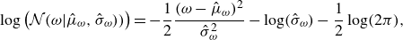 \begin{equation} \log \left ( \mathcal{N} (\omega | \hat {\mu }_{\omega } , \hat {\sigma }_{\omega })) \right ) = -\frac {1}{2} \frac {(\omega - \hat {\mu }_{\omega })^2}{\hat {\sigma }_{\omega }^2} - \log (\hat {\sigma }_{\omega }) - \frac {1}{2} \log (2 \pi ), \end{equation}
where $\omega$
denotes the true vorticity,
$\omega$
denotes the true vorticity, $\hat {\mu }_{\omega }$
is the predicted mean of the vorticity and
$\hat {\mu }_{\omega }$
is the predicted mean of the vorticity and $\hat {\sigma }_{\omega }^2$
represents the predicted variance at each pixel. This log likelihood is then averaged over all pixels to provide a global measure of the prediction quality; large values of this averaged log likelihood indicate two qualities: that the overall uncertainty is small and that the true vorticity falls within the uncertainty bounds. The log likelihood encapsulates both the reconstruction error from the learned operators and the uncertainty inherent in the predicted latent variables due to noisy measurements. To isolate and analyse these two sources of error, we perform a bias-variance decomposition of the prediction error. This decomposition – defined as the following equation – enables a more detailed assessment by separating the deterministic error (bias) from the stochastic variability (variance) in the predicted latent states:
$\hat {\sigma }_{\omega }^2$
represents the predicted variance at each pixel. This log likelihood is then averaged over all pixels to provide a global measure of the prediction quality; large values of this averaged log likelihood indicate two qualities: that the overall uncertainty is small and that the true vorticity falls within the uncertainty bounds. The log likelihood encapsulates both the reconstruction error from the learned operators and the uncertainty inherent in the predicted latent variables due to noisy measurements. To isolate and analyse these two sources of error, we perform a bias-variance decomposition of the prediction error. This decomposition – defined as the following equation – enables a more detailed assessment by separating the deterministic error (bias) from the stochastic variability (variance) in the predicted latent states:
 \begin{equation} \mathbb{E} \big[(\hat {\boldsymbol{q}} - \boldsymbol{q})^2 \big] = ( \mathbb{E} [\hat {\boldsymbol{q}} - \boldsymbol{q} ] )^2 + \mathbb{E} \big[(\mathbb{E}[\hat {\boldsymbol{q}}] - \hat {\boldsymbol{q}})^2 \big]. \end{equation}
Here, $\hat {\boldsymbol{q}}$
denotes the reconstructed samples obtained by decoding latent variables drawn from the learned predictive distribution
$\hat {\boldsymbol{q}}$
denotes the reconstructed samples obtained by decoding latent variables drawn from the learned predictive distribution $\pi _u(\boldsymbol{y}|\boldsymbol{x},\unicode{x1D653},\unicode{x1D654}\kern2pt)$
, and
$\pi _u(\boldsymbol{y}|\boldsymbol{x},\unicode{x1D653},\unicode{x1D654}\kern2pt)$
, and $\boldsymbol{q}$
refers to the corresponding ground truth data in a given state space (e.g. vorticity, or lift space). The expectation is taken over the latent distribution. The left-hand side of the equation corresponds to the mean squared error (MSE), which quantifies the total prediction error. The first term on the right-hand side captures the squared bias, representing the deterministic error between the mean prediction and the true value, while the second term reflects the statistical variance arising from uncertainty in the predictive distribution. The bias error reflects the cumulative contribution of all learned operators, namely the decoder and the pressure network, in the reconstruction pipeline. In this study, aleatoric and epistemic uncertainties can be quantified independently for any variable of interest, including the latent vector, lift force and vorticity field.
$\boldsymbol{q}$
refers to the corresponding ground truth data in a given state space (e.g. vorticity, or lift space). The expectation is taken over the latent distribution. The left-hand side of the equation corresponds to the mean squared error (MSE), which quantifies the total prediction error. The first term on the right-hand side captures the squared bias, representing the deterministic error between the mean prediction and the true value, while the second term reflects the statistical variance arising from uncertainty in the predictive distribution. The bias error reflects the cumulative contribution of all learned operators, namely the decoder and the pressure network, in the reconstruction pipeline. In this study, aleatoric and epistemic uncertainties can be quantified independently for any variable of interest, including the latent vector, lift force and vorticity field.
In the sensor-based prediction performed by the network $\mathcal{F}_p$
, the Rectified Linear Unit (ReLU) activation function is used for its ability to introduce nonlinearity while effectively avoiding the restricted uncertainty range often associated with TanH activation. Again, 80 % of the data are allocated for training, while the remaining 20 % are used for validation and testing. To optimise training and prevent overfitting, Early Stopping is incorporated to stop training if there is no improvement in validation loss for 500 consecutive epochs. After experimentation, a regularisation constant of
$\mathcal{F}_p$
, the Rectified Linear Unit (ReLU) activation function is used for its ability to introduce nonlinearity while effectively avoiding the restricted uncertainty range often associated with TanH activation. Again, 80 % of the data are allocated for training, while the remaining 20 % are used for validation and testing. To optimise training and prevent overfitting, Early Stopping is incorporated to stop training if there is no improvement in validation loss for 500 consecutive epochs. After experimentation, a regularisation constant of $10^{-7}$
and a dropout rate of
$10^{-7}$
and a dropout rate of $0.05$
were identified as optimal, yielding the highest average likelihood during training.
$0.05$
were identified as optimal, yielding the highest average likelihood during training.
3. Results
Viscous flow over a NACA 0012 airfoil is simulated using the immersed layers method proposed by Eldredge (Reference Eldredge2022), both in the presence and absence of disturbances. Detailed descriptions of the flow solver and data generation process are provided in § 2.1. The simulation covers 105 cases, resulting in a dataset of 78 225 snapshots (points), with 3 725 points corresponding to base cases and the remainder to random disturbed flow cases. For estimation using DL, we collect the vorticity field $\boldsymbol{\omega }$
, lift coefficient
$\boldsymbol{\omega }$
, lift coefficient $C_L$
, pressure coefficient
$C_L$
, pressure coefficient $C_p$
and the coordinates of surface pressure sensors
$C_p$
and the coordinates of surface pressure sensors $(x_{sens}, y_{sens})$
. We deploy 11 evenly spaced sensors on both sides of the airfoil, as shown in figure 1. Stacked with their locations and the encoded angle of attack, the input measurement vector
$(x_{sens}, y_{sens})$
. We deploy 11 evenly spaced sensors on both sides of the airfoil, as shown in figure 1. Stacked with their locations and the encoded angle of attack, the input measurement vector $\boldsymbol{p}_{stacked}$
has a dimension of
$\boldsymbol{p}_{stacked}$
has a dimension of $38$
.
$38$
.
To gain a deep understanding of sensor response and accurately identify the regions most affected by gust interactions, a more detailed analysis is necessary. This detailed assessment will be addressed in subsequent discussions within this section.
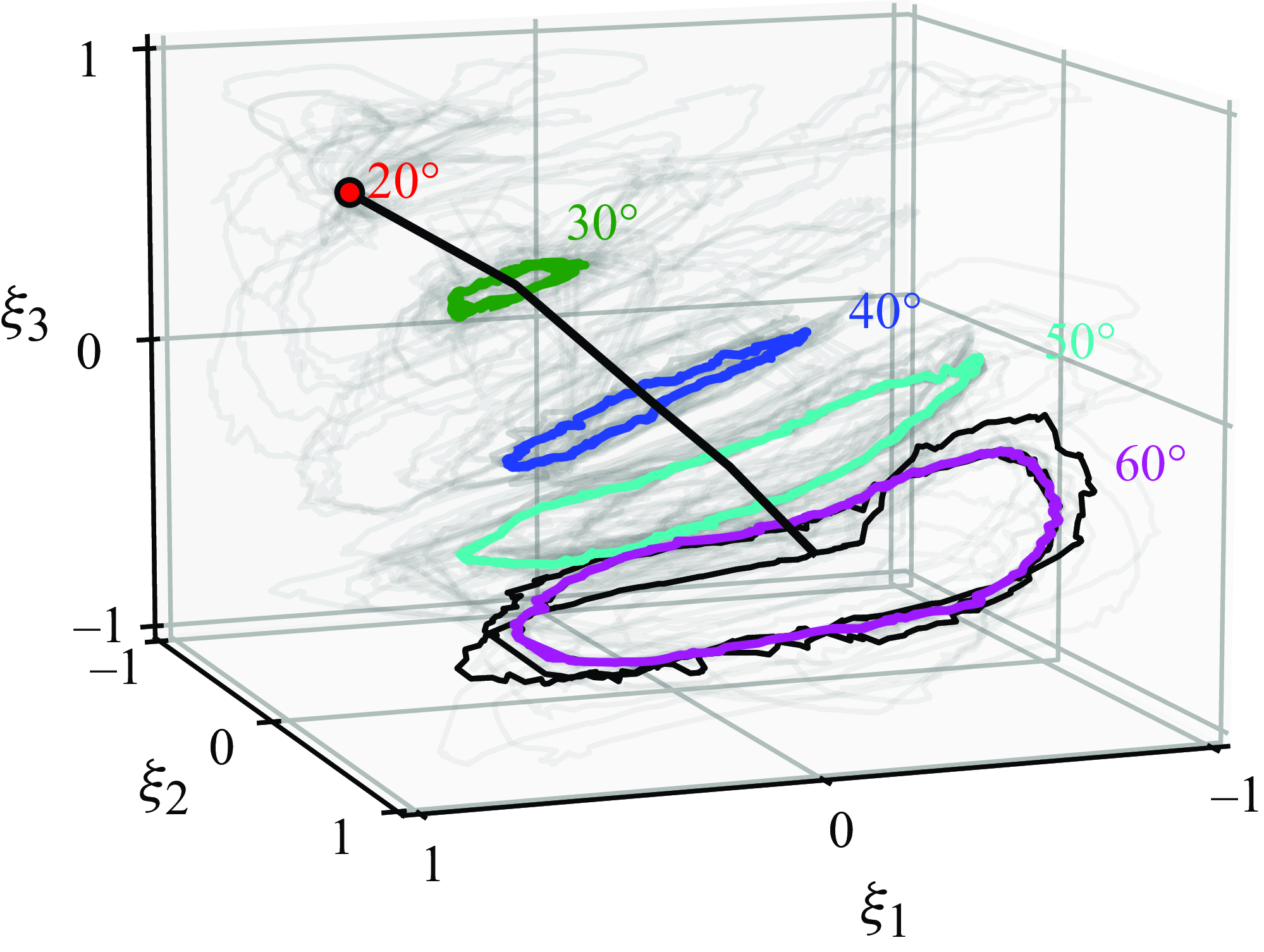
Low-order representation of flow data is presented with undisturbed cases highlighted in colour for five AoAs. The light grey paths indicate disturbed cases with the black path highlighting one of them. The black path illustrates the AoA axis.
3.1. Extracting low-order representation of flow
To manage computational expenses associated with uncertainty quantification, we initially reduce the dimensionality of the collected flow data via the lift-augmented autoencoder. The results are presented in figure 3. It displays the projected flow field in a three-dimensional latent space, illustrating the discrete pathlines for each case. This projection demonstrates the distinguishability of different cases in three-dimensional space. Notably, a curve connecting the centres of all undisturbed aerodynamic trajectories – called the angle of attack (AoA) axis – traces the airfoil’s AoA, while the spread of the trajectories captures the vortical variations in the flow. The limit-cycle behaviour is evident in the trajectories, particularly in the gust cases. In these cases, the pathline deviates from the undisturbed trajectory as the gust passes over the airfoil and eventually returns to the periodic undisturbed orbit once the gust leaves the domain. This dynamic is clearly illustrated for an airfoil encountering a gust at $\alpha =60^\circ$
, as shown by the black trajectory in figure 3. The reconstruction error of the learned autoencoder defined as
$\alpha =60^\circ$
, as shown by the black trajectory in figure 3. The reconstruction error of the learned autoencoder defined as $||\boldsymbol{\omega } - \hat {\boldsymbol{\omega }}||_2/||\boldsymbol{\omega }||_2$
will be reported in the following figures.
$||\boldsymbol{\omega } - \hat {\boldsymbol{\omega }}||_2/||\boldsymbol{\omega }||_2$
will be reported in the following figures.
3.2. Sensor-based flow reconstruction
Stacked with their coordinates $(x, y)$
and the encoded AoA, the sensor readings – denoted by
$(x, y)$
and the encoded AoA, the sensor readings – denoted by $\boldsymbol{p}_{stacked}$
– are mapped to the three-dimensional latent space
$\boldsymbol{p}_{stacked}$
– are mapped to the three-dimensional latent space $\boldsymbol{\xi }$
, as illustrated on the left side in figure 2(b). These latent variables, extracted in § 3.1, correspond to the compressed flow field and lift. Given that both the inputs and outputs are vectors, we employ a MLP network to model the mapping, denoted as
$\boldsymbol{\xi }$
, as illustrated on the left side in figure 2(b). These latent variables, extracted in § 3.1, correspond to the compressed flow field and lift. Given that both the inputs and outputs are vectors, we employ a MLP network to model the mapping, denoted as $\mathcal{F}_p$
. To quantify the network’s uncertainty in its predictions, we utilise MC dropout, incorporating a dropout layer after each dense layer in the MLP network. During both training and inference, dropout layers are active to model epistemic uncertainty. Furthermore, to account for uncertainty in the input measurements, the network is trained to predict the covariance matrix in the latent space as well. The details of the procedure are described in § 2.5, and the details of the network architecture itself are provided in table 1.
$\mathcal{F}_p$
. To quantify the network’s uncertainty in its predictions, we utilise MC dropout, incorporating a dropout layer after each dense layer in the MLP network. During both training and inference, dropout layers are active to model epistemic uncertainty. Furthermore, to account for uncertainty in the input measurements, the network is trained to predict the covariance matrix in the latent space as well. The details of the procedure are described in § 2.5, and the details of the network architecture itself are provided in table 1.
In the context of MC dropout, the dropout rate $(1-p)$
is a hyperparameter that is optimised to maximise the log likelihood (or equivalently, minimise the loss given in (2.6)). Interestingly, it was observed that the dropout rate has minimal impact on the log likelihood. Consequently, a fixed dropout rate of
$(1-p)$
is a hyperparameter that is optimised to maximise the log likelihood (or equivalently, minimise the loss given in (2.6)). Interestingly, it was observed that the dropout rate has minimal impact on the log likelihood. Consequently, a fixed dropout rate of $0.05$
was selected for training the MLP network
$0.05$
was selected for training the MLP network $\mathcal{F}_p$
.
$\mathcal{F}_p$
.
3.2.1. Sensitivity analysis to flow disturbances
To analyse how sensor variations respond to disturbances in the flow structures, we identify the most informative direction within the measurement space Gramian, $\unicode{x1D63E}_{\unicode{x1D66D}}$
, as defined in (2.5). In this subsection, we aim to identify the dominant eigenvectors within the measurement space. To achieve this, we utilise the same network architecture described in table 1, but we modify the final layer to directly output the latent variables deterministically (i.e. we omit the prediction of covariance). As mentioned earlier, this network is called
$\unicode{x1D63E}_{\unicode{x1D66D}}$
, as defined in (2.5). In this subsection, we aim to identify the dominant eigenvectors within the measurement space. To achieve this, we utilise the same network architecture described in table 1, but we modify the final layer to directly output the latent variables deterministically (i.e. we omit the prediction of covariance). As mentioned earlier, this network is called $\mathcal{F}_p^d$
. This network is trained on clean data using a MSE loss function to optimise the model weights effectively. During the evaluation phase, dropout is disabled to ensure consistent predictions with the same inputs. Additionally, we approximate the integral in (2.5) through Monte Carlo sampling, employing 100 samples of noisy measurements during inference to obtain a robust estimate of the dominant eigenvectors. The measurement noise is modelled as independent and identically distributed (i.i.d) white noise with a mean of zero and a variance of
$\mathcal{F}_p^d$
. This network is trained on clean data using a MSE loss function to optimise the model weights effectively. During the evaluation phase, dropout is disabled to ensure consistent predictions with the same inputs. Additionally, we approximate the integral in (2.5) through Monte Carlo sampling, employing 100 samples of noisy measurements during inference to obtain a robust estimate of the dominant eigenvectors. The measurement noise is modelled as independent and identically distributed (i.i.d) white noise with a mean of zero and a variance of $2.5 \times 10^{-5}$
, corresponding to a measurement accuracy of
$2.5 \times 10^{-5}$
, corresponding to a measurement accuracy of $0.15\,\%$
for the maximum pressure reading. The sensor coordinates on the airfoil are assumed to be accurately measured (i.e. they are assigned zero variance). Our analysis reveals that the first two eigenmodes of the Gramian account for more than
$0.15\,\%$
for the maximum pressure reading. The sensor coordinates on the airfoil are assumed to be accurately measured (i.e. they are assigned zero variance). Our analysis reveals that the first two eigenmodes of the Gramian account for more than $99 \,\%$
of the cumulative energy spectrum of the eigenvalues. The first eigenmode indicates the direction in the measurement space that is most informative for latent vector estimation.
$99 \,\%$
of the cumulative energy spectrum of the eigenvalues. The first eigenmode indicates the direction in the measurement space that is most informative for latent vector estimation.
Periodic variation of lift and the first mode of surface pressure measurements over time for undisturbed flow at an AoA of $\alpha =60^\circ$
. The bar plot corresponds to the first eigenmode of the measurement space Gramian; each bar represents a sensor, with their order corresponding to the numbering scheme depicted in figure 1, arranged sequentially from left to right. The informative sensors numbered in the bar chart are highlighted in the vorticity contour plots.
$\alpha =60^\circ$
. The bar plot corresponds to the first eigenmode of the measurement space Gramian; each bar represents a sensor, with their order corresponding to the numbering scheme depicted in figure 1, arranged sequentially from left to right. The informative sensors numbered in the bar chart are highlighted in the vorticity contour plots.
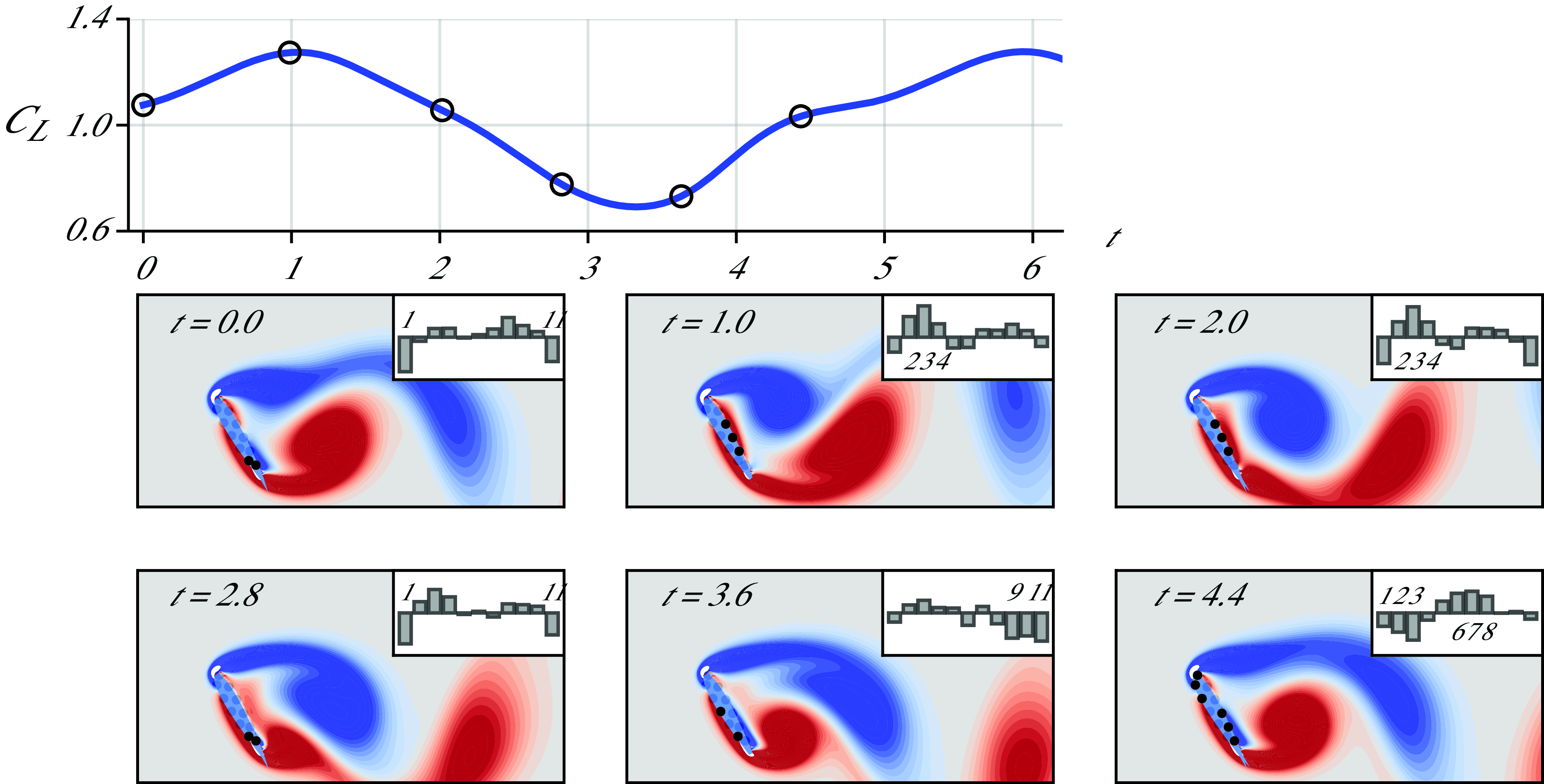
We first examine the undisturbed (base) cases for flow over an airfoil. The importance of pressure sensors in detecting flow structures around the airfoil, and the amount of information they convey, is illustrated in figure 4 for an AoA of $\alpha =60^\circ$
, exemplifying an unsteady vortex shedding case. The figure illustrates the placement of pressure sensors on the airfoil, marked by black circles. Accompanying each snapshot is a bar chart that highlights the relative importance of the pressure measurements in estimating the latent vector. This significance is derived from the first eigenmode of the Gramian matrix in the measurement space. Each bar represents a sensor, with their order corresponding to the numbering scheme depicted in figure 1: the first bar represents the sensor on the upper surface nearest the trailing edge, and the subsequent bars correspond to sensors that proceed counter-clockwise around the airfoil, culminating in the sensor closest to the trailing edge on the lower surface. The height of the bar, whether positive or negative, indicates its relative importance to estimating the latent state.
$\alpha =60^\circ$
, exemplifying an unsteady vortex shedding case. The figure illustrates the placement of pressure sensors on the airfoil, marked by black circles. Accompanying each snapshot is a bar chart that highlights the relative importance of the pressure measurements in estimating the latent vector. This significance is derived from the first eigenmode of the Gramian matrix in the measurement space. Each bar represents a sensor, with their order corresponding to the numbering scheme depicted in figure 1: the first bar represents the sensor on the upper surface nearest the trailing edge, and the subsequent bars correspond to sensors that proceed counter-clockwise around the airfoil, culminating in the sensor closest to the trailing edge on the lower surface. The height of the bar, whether positive or negative, indicates its relative importance to estimating the latent state.
According to figure 4, in the interval $t \in [0,2.8]$
a clockwise leading-edge vortex (LEV) grows, sustained by the shear layer from the leading edge. As the vortex grows to extend across the entire chord, the airfoil experiences its highest lift at
$t \in [0,2.8]$
a clockwise leading-edge vortex (LEV) grows, sustained by the shear layer from the leading edge. As the vortex grows to extend across the entire chord, the airfoil experiences its highest lift at $t = 1$
. From
$t = 1$
. From $t = 1$
through 2, the sensors 2–4 near the mid-chord of the suction side become the most impactful. This interval corresponds to the generation and extension of counter-clockwise secondary vorticity along the entire suction side. After
$t = 1$
through 2, the sensors 2–4 near the mid-chord of the suction side become the most impactful. This interval corresponds to the generation and extension of counter-clockwise secondary vorticity along the entire suction side. After $t = 2$
, the LEV begins to shed from the airfoil, and the importance of the suction-side sensors begins to diminish in favour of those on the pressure side. As the trailing-edge vortex (TEV) emerges and develops from
$t = 2$
, the LEV begins to shed from the airfoil, and the importance of the suction-side sensors begins to diminish in favour of those on the pressure side. As the trailing-edge vortex (TEV) emerges and develops from $t = 3.0$
through 3.6 and lift is at its lowest level, the sensors 9–11 on the pressure side become important. At
$t = 3.0$
through 3.6 and lift is at its lowest level, the sensors 9–11 on the pressure side become important. At $t = 4.4$
, new secondary vorticity develops under the TEV and a new vortex develops at the leading edge, and the sensors in the respective regions (1–3 and 6–8) are most informative. The cycle returns to the state at
$t = 4.4$
, new secondary vorticity develops under the TEV and a new vortex develops at the leading edge, and the sensors in the respective regions (1–3 and 6–8) are most informative. The cycle returns to the state at $t = 0$
, when the trailing-edge sensors (1 and 11) become most important.
$t = 0$
, when the trailing-edge sensors (1 and 11) become most important.
Primary mode of pressure measurements at six different snapshots as a positive gust interacts with the airfoil. Panel (a) depicts the temporal variation in lift. The spatio-temporal map of the pressure coefficient in (b), with the base flow subtracted, provides insight into how sensors respond to gust–airfoil interactions. The locations of the leading edge (LE) and trailing edge (TE) are indicated along the y-axis of the plot. Panels (c) present vorticity contours alongside sensor placements. Each bar represents a sensor indicating its value in the dominant eigenmode, with their order corresponding to the numbering scheme depicted in figure 1, arranged sequentially from left to right. The conditions are an AoA of $\alpha =60^\circ$
, and gust characteristics of (
$\alpha =60^\circ$
, and gust characteristics of ( $G=0.9$
,
$G=0.9$
, $2R/c=0.98$
,
$2R/c=0.98$
, $y_o/c=-0.06$
). The informative sensors numbered in the bar chart are highlighted in the vorticity contour plots.
$y_o/c=-0.06$
). The informative sensors numbered in the bar chart are highlighted in the vorticity contour plots.
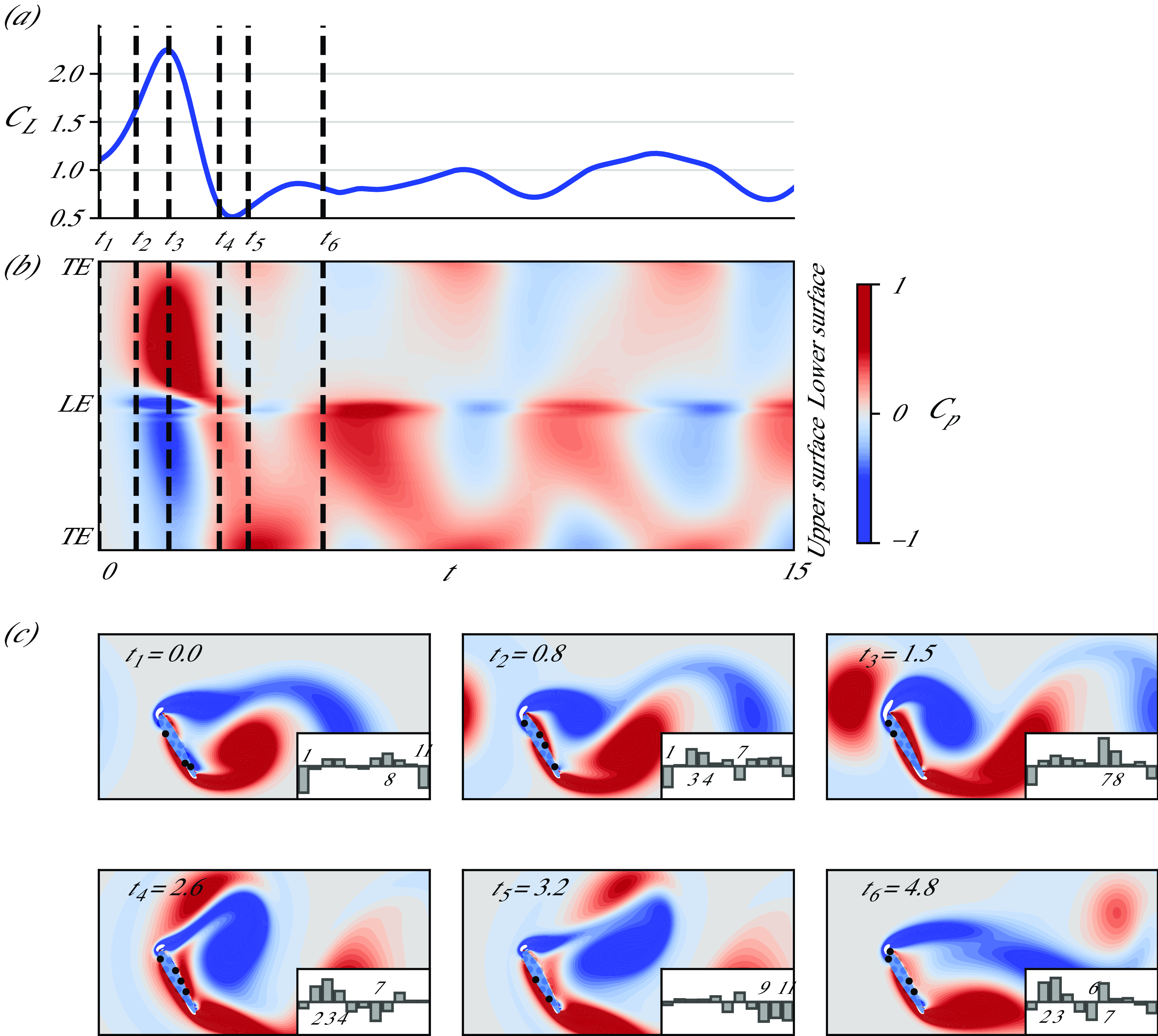
In contrast to cases at large AoAs, in which the first measurement mode varies periodically over time, at steady flow conditions – such as those for an airfoil at an AoA of $\alpha =20^\circ$
or less – we find (though omit the plots for brevity) that sensors closest to the trailing edge on either side (1 and 11) are most informative.
$\alpha =20^\circ$
or less – we find (though omit the plots for brevity) that sensors closest to the trailing edge on either side (1 and 11) are most informative.
The sensitivity of sensors to changes in the vortical structures becomes significantly more complex and transient during gust encounters over an airfoil. Figure 5(a) illustrates the evolution of lift over time for a counterclockwise (positive) disturbance. In this scenario, there is an initial increase in lift as the gust approaches the airfoil, occurring around $t_3=1.5$
. The lift force reaches its lowest point when the centre of the vortical structure aligns with the trailing edge of the airfoil, at an instant between
$t_3=1.5$
. The lift force reaches its lowest point when the centre of the vortical structure aligns with the trailing edge of the airfoil, at an instant between $t_4=2.6$
and
$t_4=2.6$
and $t_5=3.2$
. This is then followed by an increase in lift due to tail-induced effects. For a clockwise (negative) gust, the sequence of events and their impact on the lift is reversed, as shown in figure 6(a).
$t_5=3.2$
. This is then followed by an increase in lift due to tail-induced effects. For a clockwise (negative) gust, the sequence of events and their impact on the lift is reversed, as shown in figure 6(a).
Figure 5(b) illustrates a spatio-temporal distribution of the pressure coefficient for an airfoil subjected to a positive gust, with the baseline flow pressure subtracted for enhanced clarity. This visualisation highlights distinct high-pressure regions on the pressure side and low-pressure zones on the suction side of the airfoil. A striking observation emerges: the positive, counterclockwise gust disturbance distinctly imprints on the pressure field, elevating pressure on the lower surface while diminishing it on the upper surface. This effect creates a stronger upward pressure difference between the two surfaces, ultimately enhancing the lift. These findings reinforce the rationale behind our strategic placement of pressure sensors to effectively capture flow perturbations around the airfoil. The strong interaction between the gust and the LEV disrupts the typical vortex dynamics, delaying the shedding process. This disruption is evident in the periodic non-zero pressure regions observed on the map, which persist even after the gust has exited the domain. Such behaviour reflects a significant shift in the periodic vortex shedding pattern induced by the gust, underscoring the lasting impact of gust-driven disturbances on the flow field.
Primary mode of pressure measurements at six different time snapshots as a negative gust interacts with the airfoil. Panel (b) depicts the temporal variation in lift. The spatio-temporal map of the pressure coefficient in (b), with the base flow subtracted, provides insight into how sensors respond to gust–airfoil interactions. Panels (c) present vorticity contours alongside sensor placements. Each bar represents a sensor indicating its value in the dominant eigenmode, with their order corresponding to the numbering scheme depicted in figure 1, arranged sequentially from left to right. The conditions are an AoA of $\alpha =60^\circ$
, and gust characteristics of (
$\alpha =60^\circ$
, and gust characteristics of ( $G=-0.98$
,
$G=-0.98$
, $2R/c=0.77$
,
$2R/c=0.77$
, $y_o/c=-0.26$
). The informative sensors numbered in the bar chart are highlighted in the vorticity contour plots.
$y_o/c=-0.26$
). The informative sensors numbered in the bar chart are highlighted in the vorticity contour plots.
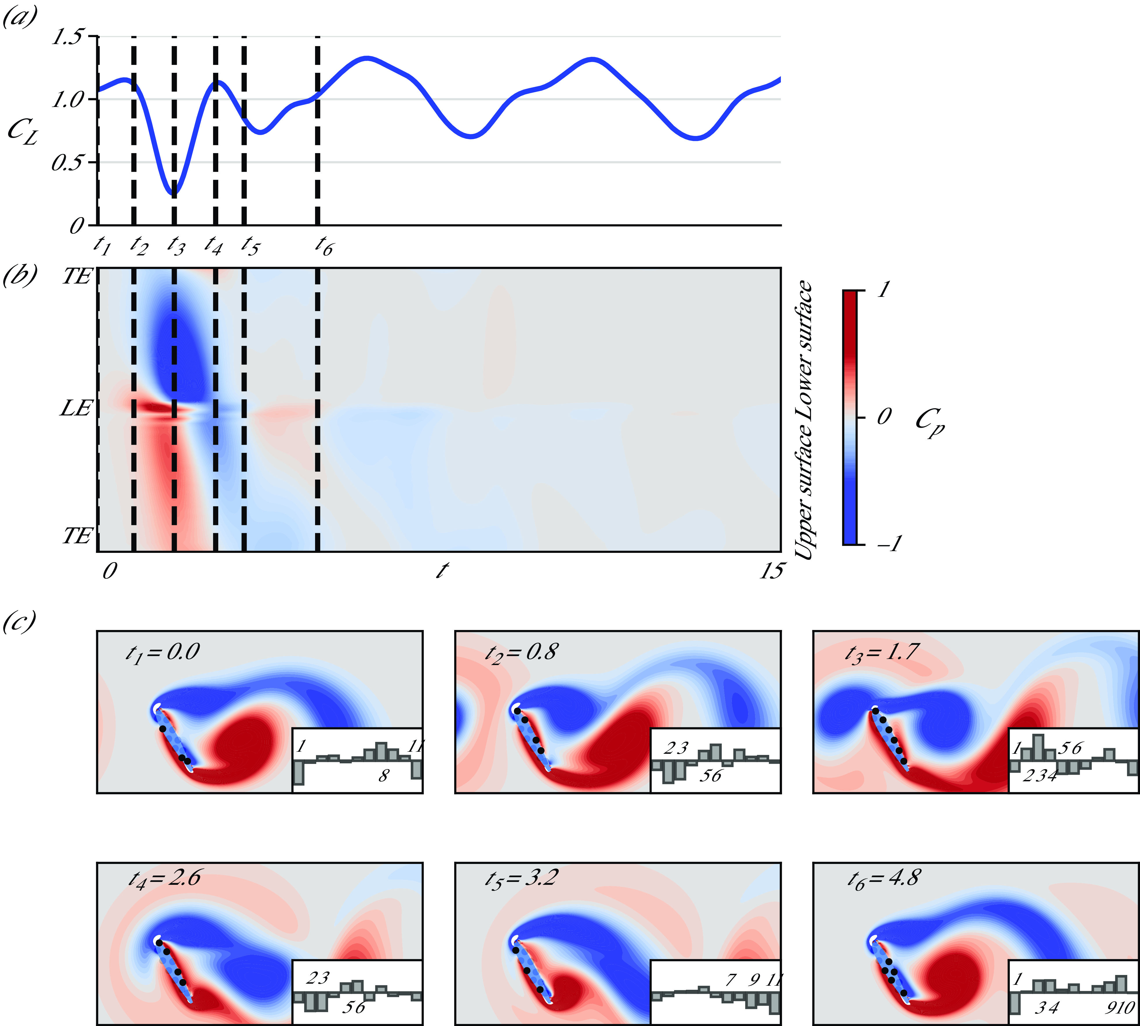
To explain some of the features we observe in the dominant eigenmodes, it is important to emphasise that the informativeness of pressure sensors as assessed by the Gramian is intrinsically tied to variations in their readings. These readings capture the evolving flow structure represented in the reduced-dimensional latent space. Consequently, the difference in the pressures across successive snapshots reflects the information conveyed in estimating flow states. Observing the vorticity fields alongside the sensor importance bars in figure 5(c), we can trace the impact of gust passage on pressure readings. When the gust tail reaches the leading edge at $t_2 = 0.8$
, nearly all sensors – particularly those near the trailing edge on the suction side and leading edge on the pressure side – register the flow changes. However, the tail’s influence is weaker compared with the dominant effects of the primary LEV and TEV. Therefore, the sensors with the highest eigenmode response remain predominantly influenced by the primary vortices, similar to the base flow case. As the gust core interacts with the airfoil and the LEV/TEV beyond
$t_2 = 0.8$
, nearly all sensors – particularly those near the trailing edge on the suction side and leading edge on the pressure side – register the flow changes. However, the tail’s influence is weaker compared with the dominant effects of the primary LEV and TEV. Therefore, the sensors with the highest eigenmode response remain predominantly influenced by the primary vortices, similar to the base flow case. As the gust core interacts with the airfoil and the LEV/TEV beyond $t_2$
, the dominant eigenmode of the pressure deviates significantly from the undisturbed scenario. At
$t_2$
, the dominant eigenmode of the pressure deviates significantly from the undisturbed scenario. At $t_3 = 1.5$
, the pressure distribution plot reveals the steepest change in time on the lower side near the leading edge, making sensors 6 and 7 the most responsive to local flow changes. The interaction between the positive gust and the LEV leads to the formation of a vortex pair with unequal strengths, which moves downstream with the flow. At this time until the gust core moves approximately one chord length away at approximately
$t_3 = 1.5$
, the pressure distribution plot reveals the steepest change in time on the lower side near the leading edge, making sensors 6 and 7 the most responsive to local flow changes. The interaction between the positive gust and the LEV leads to the formation of a vortex pair with unequal strengths, which moves downstream with the flow. At this time until the gust core moves approximately one chord length away at approximately $t_4=2.6$
, sensors on the suction side and the leading edge sensors become more informative due to substantial flow changes occurring there. When the gust core drifts further from the airfoil, sensors on the pressure side regain prominence, as seen at
$t_4=2.6$
, sensors on the suction side and the leading edge sensors become more informative due to substantial flow changes occurring there. When the gust core drifts further from the airfoil, sensors on the pressure side regain prominence, as seen at $t_5=3.2$
. Eventually, the sensor responses transition back to the periodic behaviour typical of the undisturbed flow once the gust exits the domain. During this recovery phase, the pressure distribution plot reveals a pronounced change in time on the suction surface. This is attributed to the substantial adjustments in the primary edge vortices and boundary layer on this side as the flow reverts to its baseline state.
$t_5=3.2$
. Eventually, the sensor responses transition back to the periodic behaviour typical of the undisturbed flow once the gust exits the domain. During this recovery phase, the pressure distribution plot reveals a pronounced change in time on the suction surface. This is attributed to the substantial adjustments in the primary edge vortices and boundary layer on this side as the flow reverts to its baseline state.
The evolution of the first dominant mode of the measurement space Gramian for a negative gust is in many ways similar to that of a positive gust discussed earlier. Figure 6 illustrates the variations in the pressure coefficient during the passage of the negative gust. The spatio-temporal map, which depicts the pressure coefficient with the baseline flow subtracted, reveals dynamics that is qualitatively the inverse of a positive gust. Notably, however, the gust–vortex interactions induced by the negative gust are less disruptive overall. As the negative gust approaches the airfoil, it decreases pressure on the lower surface while increasing pressure on the upper surface during the period between $t_2=0.8$
and
$t_2=0.8$
and $t_3=1.7$
. This reversal in pressure distribution creates a downward-directed pressure difference across the airfoil, ultimately reducing the lift generated by the airfoil during this interval. This distinct interaction underscores the impact of gust polarity on aerodynamic performance. When the negative gust interacts with the LEV, the vortices begin to rotate around a shared centre and eventually coalesce into a larger vortex. This merging process initiates around
$t_3=1.7$
. This reversal in pressure distribution creates a downward-directed pressure difference across the airfoil, ultimately reducing the lift generated by the airfoil during this interval. This distinct interaction underscores the impact of gust polarity on aerodynamic performance. When the negative gust interacts with the LEV, the vortices begin to rotate around a shared centre and eventually coalesce into a larger vortex. This merging process initiates around $t_3=1.7$
and concludes by
$t_3=1.7$
and concludes by $t_5=3.2$
. The resulting larger vortex intensifies the strength of the LEV, significantly affecting the pressure distribution on the suction side. Consequently, sensors 1–6, located on the upper surface of the airfoil, exhibit increased sensitivity to the localised flow changes up to
$t_5=3.2$
. The resulting larger vortex intensifies the strength of the LEV, significantly affecting the pressure distribution on the suction side. Consequently, sensors 1–6, located on the upper surface of the airfoil, exhibit increased sensitivity to the localised flow changes up to $t_5$
. As the gust core moves beyond one chord length from the airfoil, the influence on the suction side diminishes, and sensors on the pressure side regain prominence. This shift is particularly evident at
$t_5$
. As the gust core moves beyond one chord length from the airfoil, the influence on the suction side diminishes, and sensors on the pressure side regain prominence. This shift is particularly evident at $t_5$
, further marking the transition back to baseline conditions as the gust recedes from the domain. In contrast to the positive gust scenario, a negative gust does not cause a lasting delay in vortex shedding. This is apparent in the spatiotemporal map of the pressure coefficient, which reverts to baseline levels after the negative gust leaves the domain.
$t_5$
, further marking the transition back to baseline conditions as the gust recedes from the domain. In contrast to the positive gust scenario, a negative gust does not cause a lasting delay in vortex shedding. This is apparent in the spatiotemporal map of the pressure coefficient, which reverts to baseline levels after the negative gust leaves the domain.
This general trend has also been observed for the airfoil at the other four AoAs. Overall, throughout the gust–airfoil–wake interaction, nearly all sensors play a role in capturing the reduced-order flow dynamics, with their contributions varying over time based on the evolving flow structures and gust effects. This dynamic redistribution of sensor importance underscores the complexity and time-dependent nature of gust-induced disturbances. A uniform distribution of sensors across the airfoil surface is therefore recommended, as it provides robust coverage and effectively captures critical flow variations without the need for case-specific sensor tuning.
3.2.2. Aleatoric uncertainty
As described in § 2.5, to account for measurement noise in the reported predictions, we utilise the network trained with a heteroscedastic loss and active dropout, which maps surface pressure measurements to the mean and covariance matrix in the latent space representing the flow field and lift coefficient. During inference, the pressure coefficient, obtained from a high-fidelity numerical solver, is perturbed randomly along the most informative directions of the input measurements, denoted as $\boldsymbol{U}_r$
, as identified in § 2.4; at most, there are only
$\boldsymbol{U}_r$
, as identified in § 2.4; at most, there are only $r_x=2$
modes used. The noise coefficient
$r_x=2$
modes used. The noise coefficient $\zeta$
is modelled as an i.i.d white noise with zero mean and variance of
$\zeta$
is modelled as an i.i.d white noise with zero mean and variance of $2.5 \times 10^{-5}$
. We generate noisy inputs accordingly and perform
$2.5 \times 10^{-5}$
. We generate noisy inputs accordingly and perform $T=100$
forward passes through
$T=100$
forward passes through $\mathcal{F}_p$
to obtain a distribution of the mean and covariance of the latent variables. The expected value of the inferred mean over 100 samples is referred to as the predicted mean and represents the expected latent state, while the expected value of the covariance quantifies the aleatoric uncertainty of this state (see (2.12)).
$\mathcal{F}_p$
to obtain a distribution of the mean and covariance of the latent variables. The expected value of the inferred mean over 100 samples is referred to as the predicted mean and represents the expected latent state, while the expected value of the covariance quantifies the aleatoric uncertainty of this state (see (2.12)).
Predicted mean with $95 \,\%$
confidence ellipses of latent variables at a couple of instants for five undisturbed cases are shown. The solid-coloured curves represent the mean of
$95 \,\%$
confidence ellipses of latent variables at a couple of instants for five undisturbed cases are shown. The solid-coloured curves represent the mean of $\hat {\boldsymbol{\mu }}$
, while the dashed black curves indicate the true trajectories extracted from the lift-augmented autoencoder. Thicker ellipses correspond to periods of maximum uncertainty. This figure showcases aleatoric uncertainty due to inherent noise in the input measurements. The solid black path connecting the centre point of all trajectories corresponds to the AoA axis.
$\hat {\boldsymbol{\mu }}$
, while the dashed black curves indicate the true trajectories extracted from the lift-augmented autoencoder. Thicker ellipses correspond to periods of maximum uncertainty. This figure showcases aleatoric uncertainty due to inherent noise in the input measurements. The solid black path connecting the centre point of all trajectories corresponds to the AoA axis.
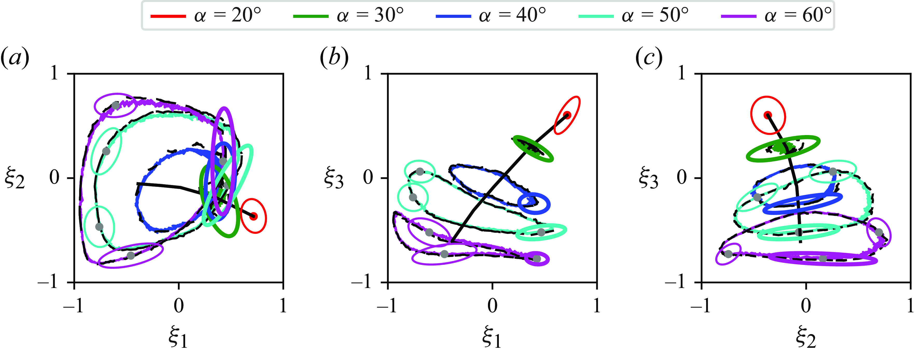
Figure 7 illustrates the trajectories of the predicted means of the latent variables alongside their $95 \,\%$
confidence ellipses at a small number of time instants, depicted in three plots representing the three coordinate planes of the latent space. These ellipses visualise the uncertainty distribution across five undisturbed cases. To compute these uncertainty bounds, we first perform a singular value decomposition (SVD) on the covariance matrix of the latent variables and then project the ellipsoid on the corresponding coordinate planes. The SVD extracts the principal axes of uncertainty, enabling us to align the ellipses along these dominant directions. The figure also includes the corresponding true trajectories extracted from the autoencoder, shown as black dashed lines for comparison. The figure clearly demonstrates that, despite the noise in the input measurements, the trained NN effectively maintains its robustness in predicting the low-dimensional representation of the flow from these measurements. The uncertainty ellipses further provide more information about the effect of measurement noise on the uncertainty in the predictions. The dominant direction of uncertainty across all AoAs primarily (during most of the time) lies perpendicular to the AoA axis, depicted as a solid black path in figure 7. This suggests that measurement noise has a significant impact on vorticity field predictions within the surrounding flow at a given AoA. Conversely, the reduced uncertainty along the AoA axis can be attributed to the encoding of the AoA alongside pressure measurements. The alignment of the major axis of the ellipses, primarily tangential to the trajectory, suggests that the estimator’s uncertainty about its predictions is most significant in the direction of preceding or subsequent snapshots. This behaviour indicates that vorticity variations between consecutive snapshots lead to sensor measurement changes that remain within the uncertainty bounds, implying reduced measurements’ sensitivity along this direction.
$95 \,\%$
confidence ellipses at a small number of time instants, depicted in three plots representing the three coordinate planes of the latent space. These ellipses visualise the uncertainty distribution across five undisturbed cases. To compute these uncertainty bounds, we first perform a singular value decomposition (SVD) on the covariance matrix of the latent variables and then project the ellipsoid on the corresponding coordinate planes. The SVD extracts the principal axes of uncertainty, enabling us to align the ellipses along these dominant directions. The figure also includes the corresponding true trajectories extracted from the autoencoder, shown as black dashed lines for comparison. The figure clearly demonstrates that, despite the noise in the input measurements, the trained NN effectively maintains its robustness in predicting the low-dimensional representation of the flow from these measurements. The uncertainty ellipses further provide more information about the effect of measurement noise on the uncertainty in the predictions. The dominant direction of uncertainty across all AoAs primarily (during most of the time) lies perpendicular to the AoA axis, depicted as a solid black path in figure 7. This suggests that measurement noise has a significant impact on vorticity field predictions within the surrounding flow at a given AoA. Conversely, the reduced uncertainty along the AoA axis can be attributed to the encoding of the AoA alongside pressure measurements. The alignment of the major axis of the ellipses, primarily tangential to the trajectory, suggests that the estimator’s uncertainty about its predictions is most significant in the direction of preceding or subsequent snapshots. This behaviour indicates that vorticity variations between consecutive snapshots lead to sensor measurement changes that remain within the uncertainty bounds, implying reduced measurements’ sensitivity along this direction.
Aleatoric (data) uncertainty of five undisturbed cases due to measurement noise, represented by the predicted mean and two standard deviations for the lift and the vorticity fields. The left column illustrates the evolution of the predicted lift coefficient alongside the ground truth for five different AoAs. The decoder’s reconstruction error in the reference vorticity field is computed to be $\approx 0.03$
for all AoAs. Symbols indicate the instants of maximum uncertainty in the predicted latent space, with the corresponding predicted vorticity field shown in the right panels. The far-right column presents the two standard deviations of the vorticity field. The term ‘ll’ refers to the average pixel-wise log likelihood of the predicted vorticity field computed by (2.15).
$\approx 0.03$
for all AoAs. Symbols indicate the instants of maximum uncertainty in the predicted latent space, with the corresponding predicted vorticity field shown in the right panels. The far-right column presents the two standard deviations of the vorticity field. The term ‘ll’ refers to the average pixel-wise log likelihood of the predicted vorticity field computed by (2.15).
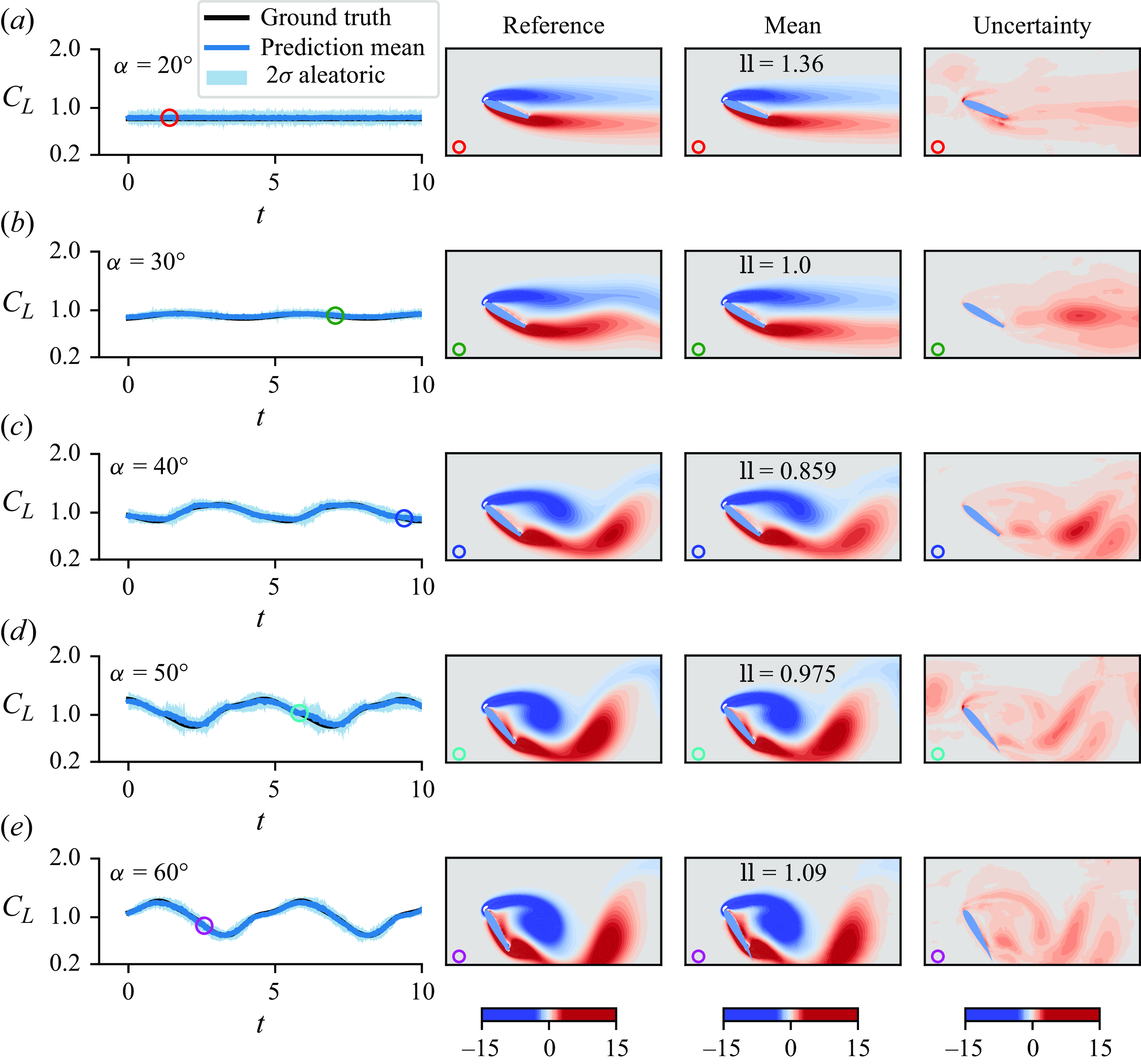
To compute the aleatoric uncertainty in the predicted flow field, we draw $M=100$
samples of the latent variables from the predicted probability distribution (2.12) computed during the evaluation phase, and used these sampled latent variables to reconstruct samples of the vorticity and lift via (2.14). The expected value and variance of the reconstructed samples indicate the characteristics of a Gaussian distribution. The left column of figure 8 presents the predicted lift history across five undisturbed cases, including the corresponding
$M=100$
samples of the latent variables from the predicted probability distribution (2.12) computed during the evaluation phase, and used these sampled latent variables to reconstruct samples of the vorticity and lift via (2.14). The expected value and variance of the reconstructed samples indicate the characteristics of a Gaussian distribution. The left column of figure 8 presents the predicted lift history across five undisturbed cases, including the corresponding $95 \,\%$
confidence interval. The predictions show high accuracy across all AoAs, with slightly wider uncertainty envelopes at
$95 \,\%$
confidence interval. The predictions show high accuracy across all AoAs, with slightly wider uncertainty envelopes at $\alpha =30^\circ , 50^\circ$
. At these specific angles, even minor perturbations in the measurements can cause the predicted latent space samples to deviate, aligning with adjacent trajectories and compromising the robustness of the results. Despite this, the actual lift measurements consistently fall within the predicted uncertainty intervals.
$\alpha =30^\circ , 50^\circ$
. At these specific angles, even minor perturbations in the measurements can cause the predicted latent space samples to deviate, aligning with adjacent trajectories and compromising the robustness of the results. Despite this, the actual lift measurements consistently fall within the predicted uncertainty intervals.
The variance of the predicted samples fluctuates over time; in the heteroscedastic model, this variance is data-dependent, changing based on the input conditions. The instants when the variance in the predicted latent variables is maximum are indicated in figure 7 with thicker ellipses. These specific times are also marked in figure 8 using coloured symbols. At these critical moments, when the predictions in the latent space exhibit considerable uncertainty, we further investigate the uncertainty in the predicted lift and vorticity fields as in figure 8. In general, the instants when the latent variables’ predictions show maximum deviation from true trajectories do not align with the highest uncertainty in the lift and vorticity predictions. This is not surprising, given the nonlinear nature of the decoder. The analysis shows that the greatest uncertainty in vorticity predictions at each snapshot occurs in the regions of the largest gradient of the vorticity field. This suggests two aspects of pressure-based estimation that deserve further study: first, the regions of large vorticity gradient also tend to coincide with dynamically important topological features, such as saddle points (Tu et al. Reference Tu, Marzanek, Green and Rival2022); also, these large-gradient regions are often associated with shear layers, where at higher Reynolds numbers, small-scale vortices and instabilities tend to form. While these smaller-scale structures introduce local turbulence, their impact on pressure readings is typically less significant than that of large-scale vortices in the wake and separation events near the airfoil itself.
To assess the estimator’s performance, we can evaluate the log likelihood at the reference vorticity by (2.15) and show it as ‘ll’ in the predicted mean panels. Interestingly, the predictions at all AoAs perform reasonably well. The high positive log-likelihood values indicate a dense concentration of predicted values around the ground truth, suggesting that the model provides accurate overall predictions for all angles under study.
Aleatoric uncertainty in gust–airfoil aerodynamics is illustrated with the predicted mean (solid-coloured curves) and a $95 \,\%$
confidence interval for lift coefficient and vorticity field. The conditions depicted are: (a)
$95 \,\%$
confidence interval for lift coefficient and vorticity field. The conditions depicted are: (a) $\alpha =30^\circ$
,
$\alpha =30^\circ$
, $G=0.93$
,
$G=0.93$
, $2R/c=0.98$
,
$2R/c=0.98$
, $y_o/c=0.04$
; (b)
$y_o/c=0.04$
; (b) $\alpha =50^\circ$
,
$\alpha =50^\circ$
, $G=0.93$
,
$G=0.93$
, $2R/c=0.68$
,
$2R/c=0.68$
, $y_o/c=0.09$
; and (c)
$y_o/c=0.09$
; and (c) $\alpha =60^\circ$
,
$\alpha =60^\circ$
, $G=-0.98$
,
$G=-0.98$
, $2R/c=0.77$
,
$2R/c=0.77$
, $y_o/c=-0.26$
(a). The light solid curves in the lift plots represent the corresponding undisturbed cases, providing a baseline for comparison. The black solid orbits in the latent space illustrate the true trajectories. Symbols indicate the instants when deviations from the mean are at their peak in the latent space, with ellipses showing the eigenmodes of these deviations. The vorticity plots show predictions at these specific times, highlighting the impact of the gust on the flow field. The decoder’s reconstruction error in the reference vorticity field is computed to be
$y_o/c=-0.26$
(a). The light solid curves in the lift plots represent the corresponding undisturbed cases, providing a baseline for comparison. The black solid orbits in the latent space illustrate the true trajectories. Symbols indicate the instants when deviations from the mean are at their peak in the latent space, with ellipses showing the eigenmodes of these deviations. The vorticity plots show predictions at these specific times, highlighting the impact of the gust on the flow field. The decoder’s reconstruction error in the reference vorticity field is computed to be $\approx 0.17$
for all AoAs.
$\approx 0.17$
for all AoAs.

We now shift our focus to gust-encounter scenarios. Figure 9 presents aerodynamic predictions for an airfoil experiencing random disturbances at three distinct AoAs: $\alpha \in \{30^\circ , 50^\circ , 60^\circ \}$
. The comparison between the predicted means (with a
$\alpha \in \{30^\circ , 50^\circ , 60^\circ \}$
. The comparison between the predicted means (with a $95 \,\%$
confidence interval) and reference data highlight several key aspects of the model’s performance during gust encounters. The presence of gusts disrupts the normally periodic behaviour of the latent space trajectories, pulling them away from their stable limit cycle. As the disturbance fades, however, the trajectories gradually return to their stable trajectory. This cyclical deviation and recovery showcase the model’s capability to capture the transient, complex nature of the gust–airfoil interaction. Despite the introduction of disturbances, the predicted means in the latent space maintain a strong alignment with the reference data at higher AoAs. However, at lower angles, particularly on the
$95 \,\%$
confidence interval) and reference data highlight several key aspects of the model’s performance during gust encounters. The presence of gusts disrupts the normally periodic behaviour of the latent space trajectories, pulling them away from their stable limit cycle. As the disturbance fades, however, the trajectories gradually return to their stable trajectory. This cyclical deviation and recovery showcase the model’s capability to capture the transient, complex nature of the gust–airfoil interaction. Despite the introduction of disturbances, the predicted means in the latent space maintain a strong alignment with the reference data at higher AoAs. However, at lower angles, particularly on the $\xi _1 - \xi _2$
plane for
$\xi _1 - \xi _2$
plane for $\alpha =30^\circ$
, the accuracy of the predictions diminishes, as evident in the larger covariance ellipse in that plane. Nevertheless, even with this degradation, the true trajectory remains within the uncertainty bounds, suggesting that the model still captures the underlying flow dynamics despite increased uncertainty. The predicted lift evolution closely tracks the reference values, with a minor deviation observed at the peak due to the passage of the gust. A key insight from the figure is the model’s capacity to effectively capture the heightened uncertainty during gust–airfoil interactions. As gusts induce more variability in the flow, the model appropriately widens the uncertainty bounds, reflecting a reduced confidence in the predictions. This expanded confidence interval is vital, as it ensures that, despite the added complexity of gust disturbances, the true values stay within the predicted uncertainty range.
$\alpha =30^\circ$
, the accuracy of the predictions diminishes, as evident in the larger covariance ellipse in that plane. Nevertheless, even with this degradation, the true trajectory remains within the uncertainty bounds, suggesting that the model still captures the underlying flow dynamics despite increased uncertainty. The predicted lift evolution closely tracks the reference values, with a minor deviation observed at the peak due to the passage of the gust. A key insight from the figure is the model’s capacity to effectively capture the heightened uncertainty during gust–airfoil interactions. As gusts induce more variability in the flow, the model appropriately widens the uncertainty bounds, reflecting a reduced confidence in the predictions. This expanded confidence interval is vital, as it ensures that, despite the added complexity of gust disturbances, the true values stay within the predicted uncertainty range.
A notable observation is the difference between disturbed and undisturbed cases: the uncertainty of the predicted latent variables during gust encounters is consistently larger than in the undisturbed flow at similar time instants. This reflects how the model captures the added complexity and instability introduced by the gusts. Additionally, comparing the uncertainty ellipses in the latent space for disturbed cases with undisturbed cases (figures 7 and 9) shows that the greatest uncertainty in the dominant directions during gusts is noticeably larger. The moment of peak uncertainty in the latent space aligns with either the gust’s approach to the airfoil or its direct interaction with it. As in undisturbed cases, the pressure measurements during disturbed aerodynamics are observed to display low sensitivity to changes in the flow structure across consecutive snapshots. At the point of maximum uncertainty in the latent space, the corresponding predicted vorticity field is shown for further analysis. The elevated uncertainty regions are predominantly located within the wake, particularly around the shear layers and high vorticity gradient regions, as well as in the vicinity of the gust. These areas are characterised by a more complex flow dynamics, driven by unsteady aerodynamic effects that introduce greater variability and challenge the model’s ability to provide accurate predictions. The reduced performance of the trained estimator in predicting the mean vorticity field at lower AoAs, specifically at $\alpha =30^\circ$
, is reflected in the deviations of the predicted latent vector from the true trajectory in the
$\alpha =30^\circ$
, is reflected in the deviations of the predicted latent vector from the true trajectory in the $\xi _1-\xi _2$
plane. These discrepancies occur in regions of the flow far from the airfoil, where the variations in vorticity have a negligible impact on the surface pressure measurements within the associated uncertainty bounds.
$\xi _1-\xi _2$
plane. These discrepancies occur in regions of the flow far from the airfoil, where the variations in vorticity have a negligible impact on the surface pressure measurements within the associated uncertainty bounds.
The decomposition of the prediction error into variance and squared bias for aleatoric samples in the vorticity space.
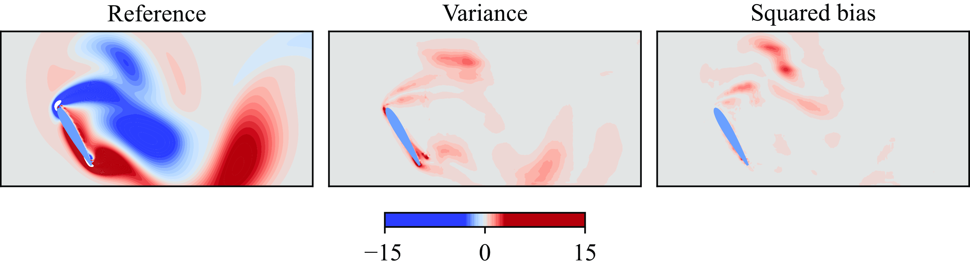
Before ending this section on statistical analysis of data uncertainty, it is important to examine the two sources of error decomposed in (2.16). Figure 10 illustrates this decomposition for the vorticity field at a representative time instant during gust–airfoil interaction. The squared bias and variance are computed after decoding each latent sample, enabling an assessment of how uncertainties in the latent space propagate to the physical field. The results show that the bias error introduced by the learned operators is concentrated primarily near the gust core and its immediate vicinity, indicating a systematic deviation between the mean reconstructed field and the ground truth. The relatively balanced magnitude of squared bias and variance across the field indicates that both deterministic and stochastic sources contribute meaningfully to the total reconstruction error. However, the presence of a localised and non-negligible bias component underscores the importance of exercising caution when interpreting the reconstructed states: predictions based solely on the mean states may systematically under- or overestimate critical flow features in regions affected by strong disturbances. On the other hand, the log likelihood defined earlier in (2.15) accounts for both sources of error in a systematic and interpretable manner, as it incorporates not only the deviation of the predicted mean from the reference field (i.e. bias) but also the uncertainty captured by the predicted covariance (i.e. variance).
3.2.3. Epistemic uncertainty
Epistemic uncertainty, stemming from incomplete knowledge about the trained DL model, is crucial in data-driven studies of gust-encounter aerodynamics. Unlike aleatoric uncertainty, epistemic uncertainty can be reduced through better models and additional data. To quantify this, in § 2.5 we described a probabilistic approach using MC dropout to sample from the model’s weights during inference. We use samples generated in the last section to estimate the model’s epistemic probability density function with (2.13), capturing both mean and covariance information through the statistics of the output samples $\{\hat {\boldsymbol{\mu }}_k\}_{k=1}^T$
. This method allows us to estimate the reliability of our predictions and refine our understanding of the transient flow fields and aerodynamic loads. In this section, we will detail our results, highlighting how MC dropout helps assess unreliability in the trained model.
$\{\hat {\boldsymbol{\mu }}_k\}_{k=1}^T$
. This method allows us to estimate the reliability of our predictions and refine our understanding of the transient flow fields and aerodynamic loads. In this section, we will detail our results, highlighting how MC dropout helps assess unreliability in the trained model.
Epistemic (model) uncertainty of estimation of five undisturbed cases. Predicted mean with $95 \,\%$
confidence ellipses of latent variables at a small number of instants for five undisturbed cases are shown. The solid-coloured curves represent the mean of
$95 \,\%$
confidence ellipses of latent variables at a small number of instants for five undisturbed cases are shown. The solid-coloured curves represent the mean of $\hat {\boldsymbol{\mu }}$
, while the dashed black curves indicate the true trajectories extracted from the lift-augmented autoencoder. Thicker ellipses correspond to periods of maximum uncertainty. The solid black path connecting the centre point of all trajectories corresponds to the AoA axis.
$\hat {\boldsymbol{\mu }}$
, while the dashed black curves indicate the true trajectories extracted from the lift-augmented autoencoder. Thicker ellipses correspond to periods of maximum uncertainty. The solid black path connecting the centre point of all trajectories corresponds to the AoA axis.

Figure 11 illustrates the estimated means of the latent variables alongside their $95 \,\%$
confidence ellipses across five undisturbed cases. This figure highlights the model’s ability to compress and predict the underlying flow dynamics accurately, despite variations in the fitted model. The ellipses, representing epistemic uncertainty, highlight the degree of imprecision arising from the model’s inherent knowledge gaps or limitations due to insufficient data. The major axes of these ellipses are predominantly perpendicular to the trajectories, reflecting the scarcity of training data away from the primary trajectory paths. These broader uncertainty regions reveal the model’s performance in terms of the epistemic uncertainty, especially when it encounters conditions that differ from what it has been trained on, reflecting the inherent limitations of the network or data.
$95 \,\%$
confidence ellipses across five undisturbed cases. This figure highlights the model’s ability to compress and predict the underlying flow dynamics accurately, despite variations in the fitted model. The ellipses, representing epistemic uncertainty, highlight the degree of imprecision arising from the model’s inherent knowledge gaps or limitations due to insufficient data. The major axes of these ellipses are predominantly perpendicular to the trajectories, reflecting the scarcity of training data away from the primary trajectory paths. These broader uncertainty regions reveal the model’s performance in terms of the epistemic uncertainty, especially when it encounters conditions that differ from what it has been trained on, reflecting the inherent limitations of the network or data.
Epistemic (model) uncertainty of five undisturbed cases, represented by the predicted mean and two standard deviations for the lift and vorticity fields. The left panels illustrate the evolution of the predicted lift coefficient alongside the ground truth for five different AoAs. Symbols indicate the instants of maximum uncertainty in the predicted latent space, with the corresponding predicted vorticity field shown in the right panels. The far-right column presents the two standard deviations of the vorticity field. The decoder’s reconstruction error in the reference vorticity field is computed to be $\approx 0.02$
for all AoAs.
$\approx 0.02$
for all AoAs.
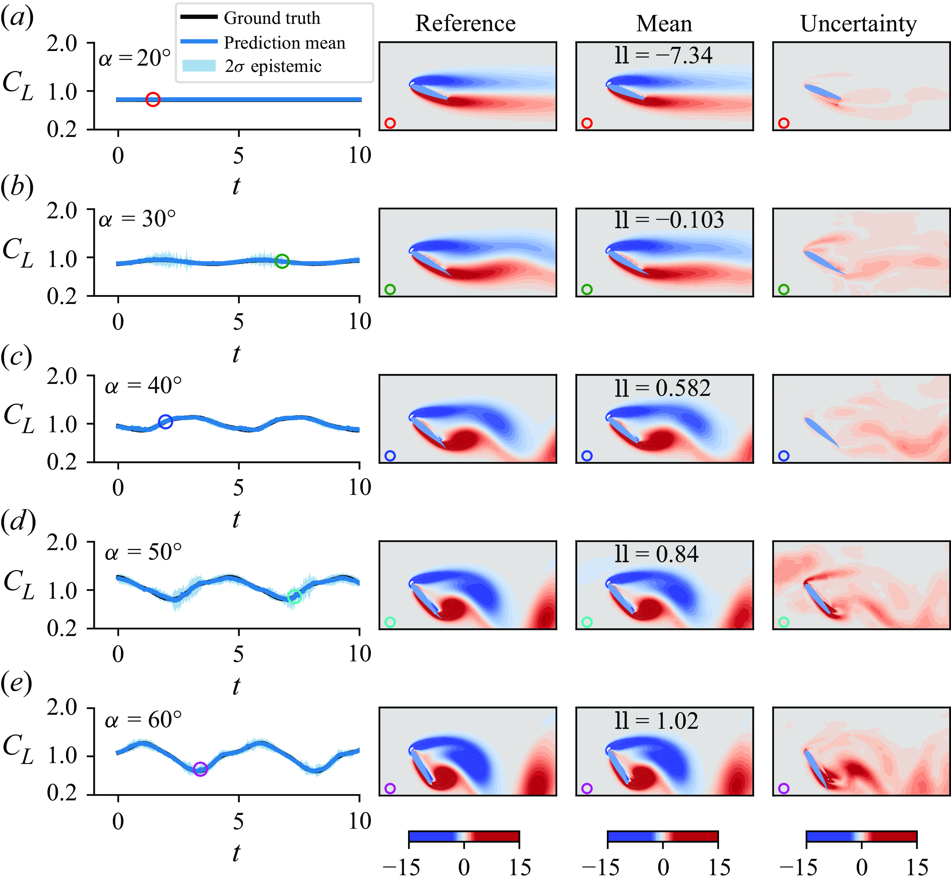
To assess the epistemic uncertainty in lift and vorticity, we draw $M=100$
samples of the latent variables from the predicted probability distribution (2.13) and reconstruct samples of vorticity via the procedure described by (2.14). The expected value and variance of the reconstructed samples indicate the characteristics of a Gaussian distribution. Figure 12 presents the mean predictions along with their
$M=100$
samples of the latent variables from the predicted probability distribution (2.13) and reconstruct samples of vorticity via the procedure described by (2.14). The expected value and variance of the reconstructed samples indicate the characteristics of a Gaussian distribution. Figure 12 presents the mean predictions along with their $95 \,\%$
confidence intervals, within which the true lift is contained. The symbols along the lift curves in figure 12 represent the snapshots when the predicted latent space samples exhibit the greatest spread around the mean (indicated by thicker ellipses in figure 11). The corresponding vorticity fields at these instants are displayed on the right, highlighting regions of maximum uncertainty in the wake. The model demonstrates significant epistemic uncertainty in regions of complex flow dynamics, particularly within regions of large vorticity gradient, such as shear layers and between vortices, which further suggests that the model would struggle most in regions of small-scale flow interactions at higher Reynolds numbers.
$95 \,\%$
confidence intervals, within which the true lift is contained. The symbols along the lift curves in figure 12 represent the snapshots when the predicted latent space samples exhibit the greatest spread around the mean (indicated by thicker ellipses in figure 11). The corresponding vorticity fields at these instants are displayed on the right, highlighting regions of maximum uncertainty in the wake. The model demonstrates significant epistemic uncertainty in regions of complex flow dynamics, particularly within regions of large vorticity gradient, such as shear layers and between vortices, which further suggests that the model would struggle most in regions of small-scale flow interactions at higher Reynolds numbers.
At lower angles such as $\alpha =20^\circ$
, the flow remains relatively steady and attached to the airfoil surface, making it easier for the model to predict the aerodynamic characteristics. At higher angles, the flow becomes fully unsteady, but the model has learned to handle these consistently unsteady patterns. The model exhibits lower confidence in its predictions in regions where the training data are sparse or underrepresented. This reduced certainty likely stems from the model’s limited exposure to the dynamics in these areas during training, making it more challenging to accurately capture and generalise the complex flow behaviour. As a result, the model’s predictive accuracy decreases, and uncertainty increases in these regions. The log likelihood per pixel is reported for the estimated vorticity field in each case, providing further insight into the model’s performance. The negative low log likelihood for
$\alpha =20^\circ$
, the flow remains relatively steady and attached to the airfoil surface, making it easier for the model to predict the aerodynamic characteristics. At higher angles, the flow becomes fully unsteady, but the model has learned to handle these consistently unsteady patterns. The model exhibits lower confidence in its predictions in regions where the training data are sparse or underrepresented. This reduced certainty likely stems from the model’s limited exposure to the dynamics in these areas during training, making it more challenging to accurately capture and generalise the complex flow behaviour. As a result, the model’s predictive accuracy decreases, and uncertainty increases in these regions. The log likelihood per pixel is reported for the estimated vorticity field in each case, providing further insight into the model’s performance. The negative low log likelihood for $\alpha =20^\circ$
is a result of the steep penalty this metric applies to deviations from the mean when the variance is small.
$\alpha =20^\circ$
is a result of the steep penalty this metric applies to deviations from the mean when the variance is small.
The analysis in figure 11 showed that the dominant uncertainty spans all three directions within the latent space across all cases. The uncertainty along the AoA axis reflects uncertainty in the AoA. This is particularly notable in the covariance ellipses for $\alpha \in \{40^\circ , 50^\circ , 60^\circ \}$
, which overlap with the mean trajectories of neighbouring angles in the latent space. This multidirectional uncertainty suggests that randomness in the model weights gives rise to large variations in the vorticity predictions not only far from the airfoil (where uncertainty perpendicular to the AoA axis plays a prominent role, as in the case of aleatoric uncertainty), but also adjacent to it (where AoA uncertainty is most influential). Indeed, the uncertainty plots of the predicted vorticity field presented in figure 12 illustrate the estimator’s confusion regarding the vorticity field adjacent to the airfoil at the specified AoAs, moreso than in the case of aleatoric uncertainty.
$\alpha \in \{40^\circ , 50^\circ , 60^\circ \}$
, which overlap with the mean trajectories of neighbouring angles in the latent space. This multidirectional uncertainty suggests that randomness in the model weights gives rise to large variations in the vorticity predictions not only far from the airfoil (where uncertainty perpendicular to the AoA axis plays a prominent role, as in the case of aleatoric uncertainty), but also adjacent to it (where AoA uncertainty is most influential). Indeed, the uncertainty plots of the predicted vorticity field presented in figure 12 illustrate the estimator’s confusion regarding the vorticity field adjacent to the airfoil at the specified AoAs, moreso than in the case of aleatoric uncertainty.
Epistemic uncertainty in gust–airfoil aerodynamics is illustrated with the predicted mean (solid-coloured curves) and a $95 \,\%$
confidence interval for lift coefficient and vorticity field. The conditions depicted are: (a)
$95 \,\%$
confidence interval for lift coefficient and vorticity field. The conditions depicted are: (a) $\alpha =30^\circ$
,
$\alpha =30^\circ$
, $G=0.93$
,
$G=0.93$
, $2R/c=0.98$
,
$2R/c=0.98$
, $y_o/c=0.04$
; (b)
$y_o/c=0.04$
; (b) $\alpha =50^\circ$
,
$\alpha =50^\circ$
, $G=0.93$
,
$G=0.93$
, $2R/c=0.68$
,
$2R/c=0.68$
, $y_o/c=0.09$
; and (c)
$y_o/c=0.09$
; and (c) $\alpha =60^\circ$
,
$\alpha =60^\circ$
, $G=-0.98$
,
$G=-0.98$
, $2R/c=0.77$
,
$2R/c=0.77$
, $y_o/c=-0.26$
. The light solid curves in the lift plots represent the corresponding undisturbed cases, providing a baseline for comparison. The black solid orbits in the latent space illustrate the true trajectories. Symbols indicate the instants of greatest deviation from the mean in the latent space, with ellipses showing the eigenmodes of these deviations. The vorticity plots show predictions at these specific times, highlighting the impact of the gust on the flow field. The decoder’s reconstruction error in the reference vorticity field is computed to be
$y_o/c=-0.26$
. The light solid curves in the lift plots represent the corresponding undisturbed cases, providing a baseline for comparison. The black solid orbits in the latent space illustrate the true trajectories. Symbols indicate the instants of greatest deviation from the mean in the latent space, with ellipses showing the eigenmodes of these deviations. The vorticity plots show predictions at these specific times, highlighting the impact of the gust on the flow field. The decoder’s reconstruction error in the reference vorticity field is computed to be $\approx 0.15$
for all AoAs.
$\approx 0.15$
for all AoAs.
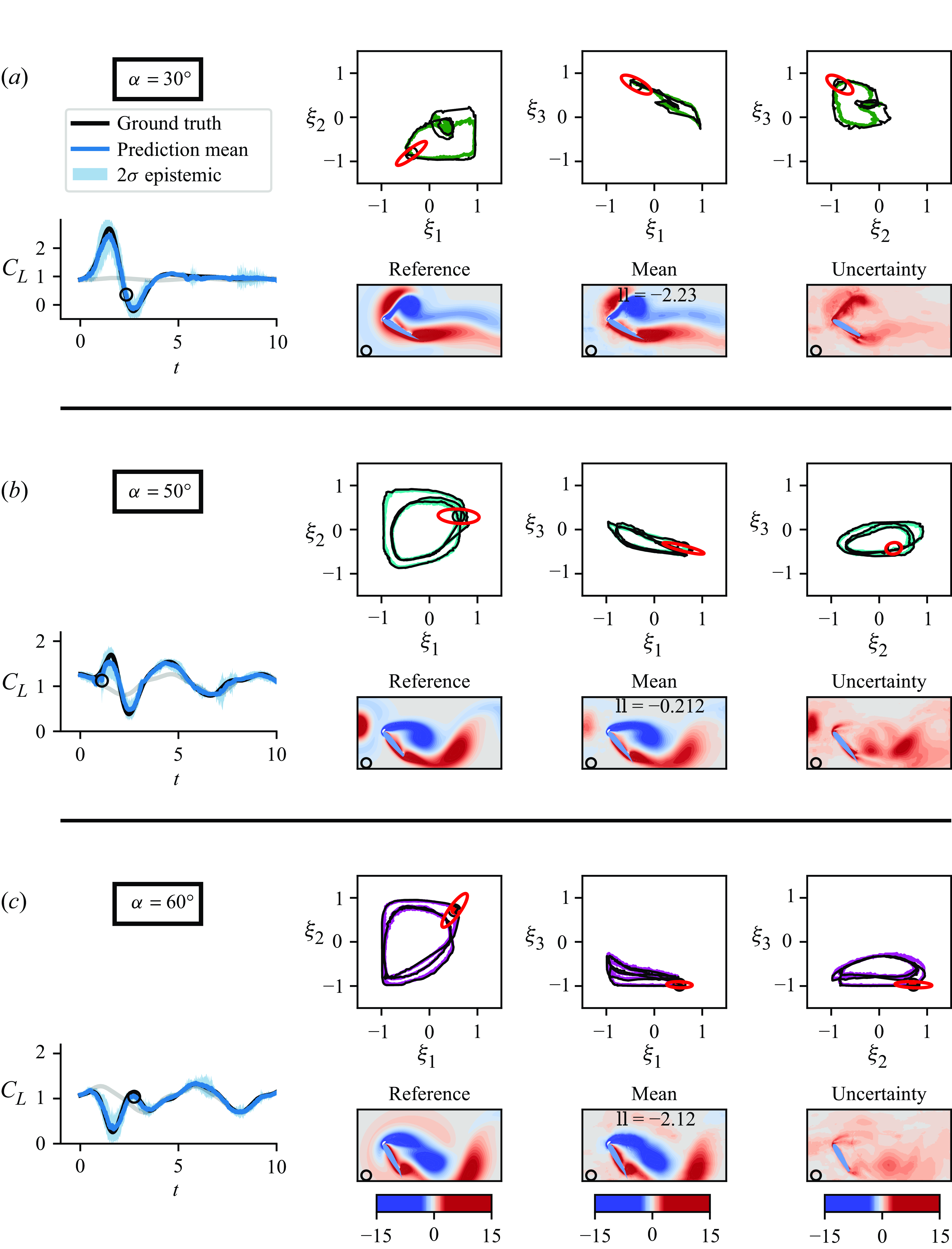
In figure 13 we investigate the epistemic uncertainty of the model’s performance in gusty aerodynamics under the same conditions as in figure 9. The predicted mean lift closely aligns with the ground truth in all cases. Similar to aleatoric uncertainty, the model exhibits greater epistemic uncertainty in its latent space predictions for disturbed cases compared with base cases. This behaviour can be attributed to the higher number of training samples corresponding to undisturbed flows, as each gust case contains intervals that revert to the underlying periodic orbit once the gust has exited the domain. As a result, the model gains more exposure to the base flow dynamics, leading to lower uncertainty in those regions. The instant when the norm of the uncertainty ellipse is maximum is depicted in the latent space. This instant is primarily linked to the gust’s approach or interaction with the airfoil. Notably, the point of maximum uncertainty in the latent variables does not always coincide with the peak variance in lift or vorticity due to the nonlinearity of the decoder. Similar to aleatoric uncertainty modelling, the model shows the highest uncertainty during gust–airfoil interactions, especially around the first lift peak, due to the highly complex aerodynamic behaviour. The mean of the estimated vorticity clearly indicates the disturbance, and the model also identifies it through a region of heightened uncertainty in its predictions. When a gust approaches and interacts with the wake, the model shows increased uncertainty not only at vortex boundaries but also at the disturbance location, highlighting its awareness of the complex flow interactions and the presence of a gust.
4. Conclusion
This study has developed a DL approach for reconstructing gust-encounter flow fields and lift coefficients and their respective uncertainties using sparse and noisy surface pressure measurements. We have demonstrated the approach on undisturbed and disturbed two-dimensional low Reynolds number flow about an airfoil at a variety of AoAs. By employing a nonlinear lift-augmented autoencoder, we effectively reduced the high-dimensional flow data to three latent components, greatly minimising the computational demands for sensor-based estimation. Our investigation has offered an in-depth analysis of how sensors dynamically respond to gust–airfoil interactions, revealing the transient importance of sensors in different positions on the airfoil surface during gust encounters.
It was observed that during the interaction of a gust, regardless of its polarity, with an edge vortex, sensors located on the upper surface of the airfoil as well as leading-edge sensors consistently captured critical information about the localised flow changes. This dominance persisted as the gust traversed up to a distance of approximately one chord length from the airfoil. Beyond this point, the influence of the gust shifted, with sensors on the lower side becoming the primary indicators of flow variations. Once the gust moved far away from the airfoil, the transient sensor responses gradually returned to their periodic behaviour, characteristic of the undisturbed flow conditions. The transient response of surface-mounted sensors indicates that a uniform distribution along the airfoil is effective for covering the most informative flow regions throughout gust interactions. Investigating the impact of sensor dropout or non-uniform sensor placement remains an important direction for future research. In the event of a sensor failure, its contribution can be effectively suppressed during inference by either omitting the corresponding input or artificially increasing its noise level to reflect its unreliability.
To effectively manage the uncertainties inherent in DL models, we employed strategies to model both aleatoric and epistemic uncertainties. Aleatoric uncertainty, arising from sensor measurement noise, was addressed using a heteroscedastic loss to predict the parameters of a multivariate normal distribution in the latent space. The directions of the greatest uncertainty in the covariance ellipsoid in the latent space were found to be nearly tangent to the latent variable trajectories, indicating that the estimator’s uncertainty is most pronounced in the direction of preceding or subsequent snapshots.
Epistemic uncertainty, stemming from the model’s dearth of training, was tackled using MC dropout to capture uncertainty in the model itself. Unlike aleatoric uncertainty, epistemic uncertainty is most significant in directions perpendicular to the latent variable trajectories, which correspond to regions with less training data. The stochasticity of both the model and the pressure readings results in high uncertainty when predicting compressed representation of the flow, lift and vorticity fields, particularly during gust–airfoil interactions. For both types of uncertainty, the highest levels of uncertainty in the predicted vorticity were observed at the vortex boundaries, where small-scale vortices and shear instabilities tend to develop at higher Reynolds numbers. We hypothesise that these small-scale structures would likely have a minimal impact on pressure sensor readings and the trained model compared with the larger-scale flow phenomena that emerge from flow separation and subsequent vortex shedding around the airfoil.
The results have demonstrated the effectiveness of our approach in accurately quantifying uncertainties within complex aerodynamic environments, all while maintaining computational efficiency. This highlights its potential to significantly enhance sensor-based flow field estimations. The uncertainty analysis presented highlights the vital importance of addressing both aleatoric and epistemic uncertainties to achieve robust and reliable predictions, particularly in complex aerodynamic environments. This uncertainty quantification can be leveraged to improve model performance. For example, by strategically employing active learning, data sampling can be concentrated in the dominant directions of uncertainty, thereby efficiently reducing model uncertainty and enhancing predictive accuracy. This approach not only strengthens the reliability of the model but also optimises resource utilisation in data acquisition.
There are a number of other aspects of this study to pursue further. We have observed the largest uncertainty in regions of high vorticity gradients. These regions often coincide with kinematically important features such as saddle points, and it would be useful to further explore this connection more deeply (Tu et al. Reference Tu, Marzanek, Green and Rival2022). Also, while the current study employed synthetic sensor data with added Gaussian noise, the model’s performance should be validated with real-time sensor measurements and experimental flow data. Moreover, the versatility of this approach allows for its application beyond aerodynamics, potentially broadening its impact across various domains. While our method requires an offline training phase that includes hyperparameter tuning and network optimisation, this cost is a one-time investment that enables real-time prediction capabilities. Once trained, the model infers flow fields and aerodynamic loads orders of magnitude faster than traditional full-order solvers, making it highly suitable for embedded, online and control-oriented applications. Furthermore, the trained model is lightweight and easily deployable on edge computing hardware, and the hyperparameter search process can be partially automated using standard tools. This trade-off between offline cost and online efficiency ensures that the framework remains practical and scalable for real-world implementations.
Given the sequential nature of both the state and observation spaces, an alternative approach would be to employ recurrent neural networks, such as long short-term memory networks (LSTMs) or gated recurrent units (GRUs), to perform flow estimation when the full temporal sequence of pressure measurements is available. Building on this idea, we are currently extending our framework to incorporate sequential filtering for real-time estimation of aerodynamic states as new pressure data become available.
Funding
This work was supported by the National Science Foundation under Award No. 2247005. The authors gratefully acknowledge this support.
Declaration of interests
The authors report no conflict of interest.
Code availability statement
The code supporting the findings of this study is openly available in the repository LowOrderFlowUQ on GitHub at https://github.com/haniehmsv/LowOrderFlowUQ/tree/main.


 Open access