


1. Introduction
1.1. The KP and FDKP equations
The full-dispersion Kadomtsev–Petviashvili (FDKP) equation
 \begin{equation}
u_t + m(\mathbf{D}) u_x + 2 u u_x = 0,
\end{equation}
\begin{equation}
u_t + m(\mathbf{D}) u_x + 2 u u_x = 0,
\end{equation}where the Fourier multiplier  $m$ is given by
 \begin{equation*}m(\mathbf{D}) = \left( 1 + \beta |\mathbf{D}|^2 \right)^{\frac{1}{2}} \left( \frac{\tanh |\mathbf{D}|}{|\mathbf{D}|} \right)^{\frac{1}{2}} \left( 1 + \frac{2\mathrm{D}_2^2}{\mathrm{D}_1^2} \right)^{\frac{1}{2}}\end{equation*}
with  $\mathbf{D} = -\mathrm{i}(\partial_x, \partial_y)$, was introduced by Lannes [Reference Lannes12] (see also Lannes and Saut [Reference Lannes and Saut13]) as an alternative to the classical Kadomtsev–Petviashvili (KP) equation
 \begin{equation}
(\zeta_t-2\zeta\zeta_x+\tfrac{1}{2}(\beta-\tfrac{1}{3})\zeta_{xxx})_x -\zeta_{yy}=0,
\end{equation}
\begin{equation}
(\zeta_t-2\zeta\zeta_x+\tfrac{1}{2}(\beta-\tfrac{1}{3})\zeta_{xxx})_x -\zeta_{yy}=0,
\end{equation}which arises as a weakly nonlinear approximation for three-dimensional gravity-capillary water waves. The parameter  $\beta \gt 0$ measures the relative strength of surface tension; the case $\beta \gt \frac{1}{3}$ for strong surface tension is termed KP-I, while the case $\beta \lt \frac{1}{3}$ for weak surface tension is KP-II. The analogous convention is used for the FDKP equation, giving us an FDKP-I equation for the strong surface tension case studied in this paper.
An FDKP solitary wave is a nontrivial, evanescent solution of (1.1) of the form  $u(x,y,t)=u(x-ct,y)$ with wave speed $c \gt 0$, that is, a localized solution of the equation
 \begin{equation}
-c u + m(\mathbf{D})u + u^2 = 0.
\end{equation}
\begin{equation}
-c u + m(\mathbf{D})u + u^2 = 0.
\end{equation} Similarly, a KP solitary wave is a nontrivial, evanescent solution of (1.2) of the form  $\zeta(x,y,t)=\zeta(x-\tilde{c}t,y)$ with wave speed $\tilde{c} \gt 0$, that is, a localized solution of the equation
 \begin{equation}
(\tilde{c} -1)\zeta + \tilde{m}(\mathbf{D})\zeta + \zeta^2 = 0,
\end{equation}
\begin{equation}
(\tilde{c} -1)\zeta + \tilde{m}(\mathbf{D})\zeta + \zeta^2 = 0,
\end{equation}where
 \begin{equation*}
\tilde{m}(\mathbf{D}) = 1+\frac{\mathrm{D}_2^2}{\mathrm{D}_1^2} + \tfrac{1}{2}(\beta- \tfrac{1}{3})\mathrm{D}_1^2.
\end{equation*}
\begin{equation*}
\tilde{m}(\mathbf{D}) = 1+\frac{\mathrm{D}_2^2}{\mathrm{D}_1^2} + \tfrac{1}{2}(\beta- \tfrac{1}{3})\mathrm{D}_1^2.
\end{equation*} Let us emphasize that these waves are fully localized, that is, decaying in all spatial directions. The KP equation allows a scaling, such that the wave speed  $\tilde{c}$ can be normalized to unity by the transformation $\zeta(x,y) \mapsto \tilde{c}\zeta(\tilde{c}^\frac{1}{2}x,\tilde{c}y)$, which converts (1.4) into the equation
 \begin{equation}
\tilde{m}(\mathbf{D})\zeta + \zeta^2 = 0.
\end{equation}
\begin{equation}
\tilde{m}(\mathbf{D})\zeta + \zeta^2 = 0.
\end{equation} While it is known that the KP-II equation does not admit any solitary waves (see de Bouard and Saut [Reference de Bouard and Saut5]), the situation is rather different for the KP-I equation. Letting  $\zeta(x,y)=\zeta(\tilde{x},\tilde{y})$ with $(\tilde{x},\tilde{y})=(\frac{1}{2}(\beta-\frac{1}{3}))^{\frac{1}{2}}(x,y)$, one can write the steady KP equation (1.5) in the alternative form
 \begin{equation}
\partial_x^2 (-\partial_x^2 \zeta + \zeta +\zeta^2)+\partial_y^2 \zeta =0,
\end{equation}
\begin{equation}
\partial_x^2 (-\partial_x^2 \zeta + \zeta +\zeta^2)+\partial_y^2 \zeta =0,
\end{equation}in which we have dropped the tildes for notational simplicity. This equation has a family of explicit symmetric ‘lump’ solutions of the form
 \begin{equation}
\zeta_k^\star(x,y)=-6\partial_x^2 \log \tau_k^\star(x,y),\qquad k=1,2,\ldots,
\end{equation}
\begin{equation}
\zeta_k^\star(x,y)=-6\partial_x^2 \log \tau_k^\star(x,y),\qquad k=1,2,\ldots,
\end{equation}where  $\tau_k^\star$ is a polynomial of degree $k(k+1)$ with $\tau_k^\star(x,y)=\tau_k^\star(-x,y)=\tau_k^\star(x,-y)$ for all $(x,y) \in {\mathbb R}^2$; the first two members of the family are
 \begin{align*}
\tau_1^\star(x,y) &=x^2+y^2+3, \\
\tau_2^\star(x,y) &=x^6+3x^4y^2+3x^2y^4+y^6+25x^4+90x^2y^2+17y^4-125x^2+475y^2+1875.
\end{align*}
\begin{align*}
\tau_1^\star(x,y) &=x^2+y^2+3, \\
\tau_2^\star(x,y) &=x^6+3x^4y^2+3x^2y^4+y^6+25x^4+90x^2y^2+17y^4-125x^2+475y^2+1875.
\end{align*} Note that the KP lump solutions  $\zeta_k^\star$ are smooth, decaying rational functions, so that the same is true of their derivatives of all orders. The functions $\zeta_1^\star$ and $\zeta_2^\star$ are sketched in Figure 1.
The KP lumps  $\zeta_1^\star$ (left) and $\zeta_2^\star$ (right).

The basic lump solution  $\zeta_1^\star$ was found by Manakov et al [Reference Manakov, Zakharov, Bordag, Its and Matveev18], while the higher-order lump solutions were discovered by Pelinovskii and Stepanyants [Reference Pelinovskii and Stepanyants21] and fully classified by Galkin, Pelinovskii and Stepanyants [Reference Galkin, Pelinovskii and Stepanyants8] (see also Pelinovskii [Reference Pelinovskii19, Reference Pelinovskii20], Clarkson [Reference Clarkson3] and Clarkson and Dowie [Reference Clarkson and Dowie4]). These results have recently been reappraised by Liu and Wei [Reference Liu and Wei15] and Liu, Wei and Yang [Reference Liu, Wei and Yang16, Reference Liu, Wei and Yang17], who in particular discussed the nongeneracy of the lump solutions. Their work is summarized in the following result; see also the comments below the lemma.
(i) Every smooth, algebraically decaying solution of the KP-I equation (1.6) has the form $\zeta(x,y)=-6\partial_x^2 \log \tau(x,y)$, for some polynomial
$\tau$ of degree
$k(k+1)$ with
$k \in {\mathbb N}$ and satisfies
$|\zeta(x,y)| \lesssim (1+x^2+y^2)^{-1}$ for all
$(x,y) \in {\mathbb R}^2$.
$\zeta(x,y)=-6\partial_x^2 \log \tau(x,y)$, for some polynomial
$\tau$ of degree
$k(k+1)$ with
$k \in {\mathbb N}$ and satisfies
$|\zeta(x,y)| \lesssim (1+x^2+y^2)^{-1}$ for all
$(x,y) \in {\mathbb R}^2$.(ii) There is a unique symmetric solution
$\zeta_k^\star$ of the form (1.7) for each
$k \in {\mathbb N}$ with
$k(k+1) \leq 600$.(iii) The solutions
$\zeta_1^\star$,
$\zeta_2^\star$ are nondegenerate: the only smooth evanescent solution of the linearized equation
for
\begin{equation*}
\partial_x^2(-\partial_x^2 w +w +2 \zeta_k^\star w)+\partial_y^2w=0
\end{equation*}
$k=1$,
$2$ that is also invariant under
$w(x,y) \mapsto w(-x,y)$ and
$w(x,y) \mapsto w(x,-y)$ is
$w(x,y)=0$.


It is conjectured that part (ii) actually holds for all  $k \in {\mathbb N}$ (see Liu, Wei and Yang [Reference Liu, Wei and Yang17]); furthermore, a sketch of the proof of the nondegeneracy of $\zeta_k^\star$ for $k \geq 3$ was given by Liu, Wei and Yang [Reference Liu, Wei and Yang16], and here we accept the validity of this result. The existence of a solitary-wave solution to the FDKP-I equation was proved by Ehrnström and Groves [Reference Ehrnström and Groves7] using a variational method, and in this paper, we considerably improve our previous result by using a perturbation argument in place of constrained minimization to prove the following theorem, which establishes the existence of FDKP solitary waves ‘close’ to $\zeta_k^\star$ for all $k$ for which (iii) holds.
Theorem 1.2. For each  $k \in {\mathbb N}$ and each sufficiently small value of $\varepsilon \gt 0$, the FDKP-I equation (1.3) possesses a smooth, fully localized solitary-wave solution $u_k^\star$ of wave speed $c=1-\varepsilon^2$, which satisfies
 \begin{equation*}u_k^\star(x,y)=u_k^\star(-x,y)=u_k^\star(x,-y)\end{equation*}
for all  $(x,y) \in {\mathbb R}^2$ and
 \begin{equation}
u_k^\star(x,y)=\varepsilon^2 \zeta_k^\star(\varepsilon x,\varepsilon^2 y)+ o(\varepsilon^2)
\end{equation}
\begin{equation}
u_k^\star(x,y)=\varepsilon^2 \zeta_k^\star(\varepsilon x,\varepsilon^2 y)+ o(\varepsilon^2)
\end{equation}uniformly over  $(x,y) \in {\mathbb R}^2$.
Theorem 1.2 is proved in Sections 2–4 below.
1.2. The method
To motivate our method, it is instructive to review the formal derivation of the steady KP equation (1.5) from the steady FDKP equation (1.3). We begin with the linear dispersion relation for the time-dependent FDKP equation (1.1) with  $\beta \gt \frac{1}{3}$: the speed $c$ and wave number $k_1$ of a two-dimensional sinusoidal travelling wave train satisfy
 \begin{equation*}
c= \left( 1 + \beta |k_1|^2 \right)^{\frac{1}{2}} \left( \frac{\tanh |k_1|}{|k_1|} \right)^{\frac{1}{2}}.
\end{equation*}
\begin{equation*}
c= \left( 1 + \beta |k_1|^2 \right)^{\frac{1}{2}} \left( \frac{\tanh |k_1|}{|k_1|} \right)^{\frac{1}{2}}.
\end{equation*} The function  $k_1 \mapsto c(k_1)$, $k_1 \geq 0$ has a unique global minimum at $k_1=0$ with $c(0)=1$ (see Figure 2). Bifurcations of nonlinear solitary waves are expected whenever the linear group and phase speeds are equal, so that $c^\prime(k_1)=0$ (see Dias and Kharif [Reference Dias and Kharif6, §3]), and one therefore expects bifurcation of small-amplitude solitary waves from uniform flow with unit speed. Furthermore, observing that $m$ is an analytic function of $k_1$ and $\frac{k_2}{k_1}$ (note that $|\mathbf{k}|^2 = k_1^2 + \frac{k_2^2}{k_1^2}k_1^2$ for $\mathbf{k} = (k_1,k_2)$), one finds that
 \begin{equation}
m(\mathbf{k})=\tilde{m}(\mathbf{k}) + O(|(k_1,\tfrac{k_2}{k_1})|^4)
\end{equation}
\begin{equation}
m(\mathbf{k})=\tilde{m}(\mathbf{k}) + O(|(k_1,\tfrac{k_2}{k_1})|^4)
\end{equation}as  $(k_1,\frac{k_2}{k_1}) \to 0$. The variables $(k_1, \frac{k_2}{k_1})$ are intrinsic to the steady KP equation (1.5), and corresponding to them is the scaling
 \begin{equation}
u(x,y) = \varepsilon^2\zeta(\varepsilon x, \varepsilon^2 y).
\end{equation}
\begin{equation}
u(x,y) = \varepsilon^2\zeta(\varepsilon x, \varepsilon^2 y).
\end{equation}FKDP-I dispersion relation for two-dimensional wave trains.

Substituting the Ansatz (1.10) with assumed wave speed
 \begin{equation*}c=1-\varepsilon^2\end{equation*}
into the steady FDKP equation (1.3), one finds that, to leading order,  $\zeta$ also satisfies the normalized KP equation (1.5). We henceforth assume that $c=1-\varepsilon^2$ for $0 \lt \varepsilon \lt \varepsilon_0$, where $\varepsilon_0$ is taken small enough for all our arguments to be valid.
In the rigorous theory, we seek solutions of (1.3) in a suitable function space  $X$ and identify a corresponding phase space $Z$ for this equation. These spaces, which are defined precisely in Section 2, satisfy $X \subseteq Z \subseteq L^2({\mathbb R}^2)$. The relationship (1.9) between the symbols $m$ and $\tilde m$ suggests that the spectrum of a solitary wave $u$ is concentrated in the region $|k_1|, |\frac{k_2}{k_1}| \ll 1$. We therefore choose a fixed value of $\delta \in (0,1)$ and decompose $L^2({\mathbb R}^2)$, and hence also $X$ and $Z$, into the direct sum of subspaces of functions whose spectra are supported in the region
 \begin{equation}
C=\left\{\mathbf{k} \in {\mathbb R}^2 \colon |k_1| \leq \delta, \left|\frac{k_2}{k_1}\right| \leq \delta\right\}
\end{equation}
\begin{equation}
C=\left\{\mathbf{k} \in {\mathbb R}^2 \colon |k_1| \leq \delta, \left|\frac{k_2}{k_1}\right| \leq \delta\right\}
\end{equation}and its complement (see Figure 3), so that
 \begin{equation*}
X=\underbrace{\chi(\mathbf{D})X}_{\displaystyle = X_1} \oplus \underbrace{(1-\chi(\mathbf{D}))X}_{\displaystyle = X_2}, \qquad
Z=\underbrace{\chi(\mathbf{D})Z}_{\displaystyle = Z_1} \oplus \underbrace{(1-\chi(\mathbf{D}))Z}_{\displaystyle = Z_2},
\end{equation*}
\begin{equation*}
X=\underbrace{\chi(\mathbf{D})X}_{\displaystyle = X_1} \oplus \underbrace{(1-\chi(\mathbf{D}))X}_{\displaystyle = X_2}, \qquad
Z=\underbrace{\chi(\mathbf{D})Z}_{\displaystyle = Z_1} \oplus \underbrace{(1-\chi(\mathbf{D}))Z}_{\displaystyle = Z_2},
\end{equation*}The cone  $C = \{\mathbf{k} \in {\mathbb R}^2 \colon |k_1| \leq \delta, |\tfrac{k_2}{k_1}| \leq \delta\}$.

in which  $\chi$ is the characteristic function of $C$. Observing that $X_1$, $Z_1$ both coincide with $\chi(\mathbf{D})L^2({\mathbb R}^2)$, we equip $Z_1$ with the $L^2({\mathbb R}^2)$ norm and $X_1$ with the equivalent scaled norm
 \begin{equation}
|u_1|_\varepsilon^2 = \int_{{\mathbb R}^2} \bigg(|u_1|^2 + \varepsilon^{-2} |\mathrm{D}_1 u_1|^2 +
\varepsilon^{-2}\left|\frac{\mathrm{D}_2}{\mathrm{D}_1}u_1\right|^2\bigg)\, \mathrm{d} x\, \mathrm{d} y,
\end{equation}
\begin{equation}
|u_1|_\varepsilon^2 = \int_{{\mathbb R}^2} \bigg(|u_1|^2 + \varepsilon^{-2} |\mathrm{D}_1 u_1|^2 +
\varepsilon^{-2}\left|\frac{\mathrm{D}_2}{\mathrm{D}_1}u_1\right|^2\bigg)\, \mathrm{d} x\, \mathrm{d} y,
\end{equation}and employ a method akin to the Lyapunov–Schmidt reduction to determine  $u_2\in X_2$ as a function of $u_1\in X_1$. With $n(\mathbf{D})=m(\mathbf{D})-1$, the result is the equation
 \begin{equation*}
\varepsilon^2 u_1 + n(\mathbf{D}) u_1 {+} \chi(\mathbf{D})(u_1 + u_2(u_1))^2 =0,
\end{equation*}
\begin{equation*}
\varepsilon^2 u_1 + n(\mathbf{D}) u_1 {+} \chi(\mathbf{D})(u_1 + u_2(u_1))^2 =0,
\end{equation*}for  $u_1$ in the unit ball
 \begin{equation*}
U=\{u_1 \in X_1 \colon |u_1|_\varepsilon \leq 1\},
\end{equation*}
\begin{equation*}
U=\{u_1 \in X_1 \colon |u_1|_\varepsilon \leq 1\},
\end{equation*}of  $X_1$.
Applying the KP scaling
 \begin{equation*}u_1(x,y) = \varepsilon^2\zeta(\varepsilon x, \varepsilon^2 y)\end{equation*}
so that the spectrum of  $\zeta$ lies in the set
 \begin{equation*}
C_\varepsilon=\left\{\mathbf{k} \in {\mathbb R}^2 \colon |k_1| \leq \frac{\delta}{\varepsilon}, \left|\frac{k_2}{k_1}\right|\leq \frac{\delta}{\varepsilon}\right\},
\end{equation*}
\begin{equation*}
C_\varepsilon=\left\{\mathbf{k} \in {\mathbb R}^2 \colon |k_1| \leq \frac{\delta}{\varepsilon}, \left|\frac{k_2}{k_1}\right|\leq \frac{\delta}{\varepsilon}\right\},
\end{equation*}one obtains the reduced equation
 \begin{equation}
\varepsilon^{-2}n_\varepsilon(\mathbf{D})\zeta+\zeta
+ \chi_\varepsilon(\mathbf{D})\zeta^2 + S_\varepsilon(\zeta)=0,
\end{equation}
\begin{equation}
\varepsilon^{-2}n_\varepsilon(\mathbf{D})\zeta+\zeta
+ \chi_\varepsilon(\mathbf{D})\zeta^2 + S_\varepsilon(\zeta)=0,
\end{equation}where
 \begin{equation*}
n_\varepsilon(\mathbf{k}) = n(\varepsilon k_1, \varepsilon^2 k_2), \qquad \chi_\varepsilon(\mathbf{k}) = \chi(\varepsilon k_1, \varepsilon^2 k_2).
\end{equation*}
\begin{equation*}
n_\varepsilon(\mathbf{k}) = n(\varepsilon k_1, \varepsilon^2 k_2), \qquad \chi_\varepsilon(\mathbf{k}) = \chi(\varepsilon k_1, \varepsilon^2 k_2).
\end{equation*} The remainder term  $S_\varepsilon \colon B_M(0) \subseteq \chi_\varepsilon(\mathbf{D}) Y^1 \rightarrow \chi_\varepsilon(\mathbf{D})L^2({\mathbb R}^2)$ satisfies the estimates
 \begin{equation*}
|S_\varepsilon(\zeta)|_{L^2} \lesssim \varepsilon^2| \zeta |_{Y^1}^3, \quad
|\mathrm{d} S_\varepsilon[\zeta]|_{\mathcal L(Y^1,L^2({\mathbb R}^2))}\lesssim \varepsilon^2| \zeta |_{Y^1}^2
\end{equation*}
\begin{equation*}
|S_\varepsilon(\zeta)|_{L^2} \lesssim \varepsilon^2| \zeta |_{Y^1}^3, \quad
|\mathrm{d} S_\varepsilon[\zeta]|_{\mathcal L(Y^1,L^2({\mathbb R}^2))}\lesssim \varepsilon^2| \zeta |_{Y^1}^2
\end{equation*}(see Section 3), where
 \begin{equation*}Y^1 = \{u \in L^2({\mathbb R}^2)\colon |u|_{Y^1} \lt \infty\}, \qquad
|u|_{Y^1}^2 = \int_{{\mathbb R}^2} \bigg(|u|^2 + |\mathrm{D}_1 u|^2 +
\left|\frac{\mathrm{D}_2}{\mathrm{D}_1}u\right|^2\bigg)\, \mathrm{d} x\, \mathrm{d} y\end{equation*}
\begin{equation*}Y^1 = \{u \in L^2({\mathbb R}^2)\colon |u|_{Y^1} \lt \infty\}, \qquad
|u|_{Y^1}^2 = \int_{{\mathbb R}^2} \bigg(|u|^2 + |\mathrm{D}_1 u|^2 +
\left|\frac{\mathrm{D}_2}{\mathrm{D}_1}u\right|^2\bigg)\, \mathrm{d} x\, \mathrm{d} y\end{equation*}is the natural energy space for the KP-I equation (see de Bouard and Saut [Reference de Bouard and Saut5]); the constant  $M \gt 1$ is chosen large enough so that $\zeta_k^\star \in B_M(0)$, while the requirement that $B_M(0)$ is contained in the range of the isomorphism $u_1 \mapsto \zeta$ requires $\varepsilon \leq M^{-2}$. In the formal limit $\varepsilon \to 0$, the subspace $\chi_\varepsilon(\mathbf{D})Y^1$ ‘fills out’ all of $Y^1$ and Equation (1.13) reduces to the KP equation (1.5).
We demonstrate in Theorem 4.2 that Equation (1.13) has solutions  $\zeta_k^\varepsilon$ which satisfy $\zeta_k^\varepsilon \rightarrow \zeta_k^\star$ as $\varepsilon \rightarrow 0$ in a suitable subspace of $Y^1$, and deduce our main Theorem 1.2 by tracing back the steps in the reduction procedure. One of the key arguments is based upon the nondegeneracy result given in Lemma 1.1(iii), which allows one to apply a variant of the implicit-function theorem. For this purpose we exploit the fact that the reduction procedure preserves the invariance of Equation (1.3) under $u(x,y) \mapsto u(-x,y)$ and $u(x,y) \mapsto u(x,-y)$, so that Equation (1.13) is invariant under $\zeta(x,y) \mapsto \zeta(-x,y)$ and $\zeta(x,y) \mapsto \zeta(x,-y)$. It is necessary to use a low regularity version of the implicit-function theorem since the reduction in Section 3 is performed using the $\varepsilon$-dependent norm $|\cdot|_\varepsilon$ and thus does not yield information concerning the smoothness of $u_1$ as a function of $\varepsilon$.
Ehrnström and Groves [Reference Ehrnström and Groves7] use a variational version of the reduction procedure outlined above to reduce a variational principle for Equation (1.3) to a variational principle for (1.13) and proceed by finding critical points of the reduced variational functional by the direct methods of the calculus of variations. Here, with some amendments, we use their functional-analytic setting and follow the steps in their reduction (see Sections 2 and 3 below), but study the reduced equation (1.13) in Section 4 in an entirely different manner, arriving at a much more comprehensive conclusion.
Perturbation arguments to construct localized solutions approximated by nondegenerate KP lump solutions have recently also been used for the Gross-Pitaevskii equation by Liu et al [Reference Liu, Wang, Wei and Yang14] (see also Chiron and Scheid [Reference Chiron and Scheid2] for a numerical approach) and for the steady water-wave problem with strong surface tension by Gui et al [Reference Gui, Lai, Liu, Wei and Yang11] and Groves and Wahlén [Reference Groves and Wahlén10], who included vorticity effects. The method has additionally been applied to physical problems approximated by other model equations, in particular to the Whitham equation by Stefanov and Wright [Reference Stefanov and Wright22] (perturbation of Korteweg–de Vries solitary waves), to the gravity-capillary steady water-wave problem by Groves [Reference Groves9] (perturbation of Korteweg–de Vries and nonlinear Schrödinger solitary waves) and Buffoni, Groves and Wahlén [Reference Buffoni, Groves and Wahlén1] (perturbation of two-dimensional Schrödinger solitary waves).
2. Function spaces
In this section, we introduce the Banach spaces used in our theory and state their main properties; the proofs of most of these results are given by Ehrnström and Groves [Reference Ehrnström and Groves7, §2]. We use the familiar scale  $\{H^r({\mathbb R}^2), |\cdot|_{H^r}\}_{r \geq 0}$ of Sobolev spaces together with the anisotropic spaces
 \begin{align*}
X&=\{u \in L^2({\mathbb R}^2)\colon |u|_X \lt \infty\}, \qquad
|u|_{X}^2 = \int_{{\mathbb R}^2} \bigg( 1 + \frac{k_2^2}{k_1^2} + \frac{k_2^4}{k_1^2} + |\mathbf{k}|^{2s}\bigg) |\hat u(\mathbf{k})|^2\, \mathrm{d} \mathbf{k}, \\
Z&=\{u \in L^2({\mathbb R}^2)\colon |u|_Z \lt \infty\}, \qquad
|u|_{Z}^2 = \int_{{\mathbb R}^2} \left( 1 + |\mathbf{k}| + k_1^2|\mathbf{k}|^{2s-3}\right) |\hat u(\mathbf{k})|^2\, \mathrm{d} \mathbf{k},
\end{align*}
\begin{align*}
X&=\{u \in L^2({\mathbb R}^2)\colon |u|_X \lt \infty\}, \qquad
|u|_{X}^2 = \int_{{\mathbb R}^2} \bigg( 1 + \frac{k_2^2}{k_1^2} + \frac{k_2^4}{k_1^2} + |\mathbf{k}|^{2s}\bigg) |\hat u(\mathbf{k})|^2\, \mathrm{d} \mathbf{k}, \\
Z&=\{u \in L^2({\mathbb R}^2)\colon |u|_Z \lt \infty\}, \qquad
|u|_{Z}^2 = \int_{{\mathbb R}^2} \left( 1 + |\mathbf{k}| + k_1^2|\mathbf{k}|^{2s-3}\right) |\hat u(\mathbf{k})|^2\, \mathrm{d} \mathbf{k},
\end{align*}in which the Sobolev index  $s \gt \frac{3}{2}$ is fixed and $u \mapsto \hat{u}$ denotes the unitary Fourier transform on $L^2({\mathbb R}^2)$. We also use the scale $\{Y^r,|\cdot|_{Y^r}\}_{r \geq 0}$, where
 \begin{equation}
Y^r = \{u \in L^2({\mathbb R}^2)\colon |u|_{Y^r} \lt \infty\}, \qquad
|u|_{Y^r}^2 = \int_{{\mathbb R}^2} \bigg(1+k_1^2+\frac{k_2^2}{k_1^2}\bigg)^{\!r} |\hat u(\mathbf{k})|^2\, \mathrm{d} \mathbf{k}.
\end{equation}
\begin{equation}
Y^r = \{u \in L^2({\mathbb R}^2)\colon |u|_{Y^r} \lt \infty\}, \qquad
|u|_{Y^r}^2 = \int_{{\mathbb R}^2} \bigg(1+k_1^2+\frac{k_2^2}{k_1^2}\bigg)^{\!r} |\hat u(\mathbf{k})|^2\, \mathrm{d} \mathbf{k}.
\end{equation} Note that  $Y^0=L^2({\mathbb R}^2)$ while $Y^1$ is the natural energy space for the KP-I equation (see de Bouard and Saut [Reference de Bouard and Saut5]). Ehrnström and Groves [Reference Ehrnström and Groves7] use only the space $Y^1$, there called $\tilde{Y}$, but the proof of the following proposition is a straightforward variant of the proof of Lemma 2.1(i) in that reference.
Proposition 2.1. One has the continuous embeddings
 \begin{equation*}
Y^r \hookrightarrow L^2({\mathbb R}^2), \quad H^{s-\frac{1}{2}}({\mathbb R}^2) \hookrightarrow Z \hookrightarrow L^2({\mathbb R}^2), \quad X \hookrightarrow H^s({\mathbb R}^2)
\end{equation*}
\begin{equation*}
Y^r \hookrightarrow L^2({\mathbb R}^2), \quad H^{s-\frac{1}{2}}({\mathbb R}^2) \hookrightarrow Z \hookrightarrow L^2({\mathbb R}^2), \quad X \hookrightarrow H^s({\mathbb R}^2)
\end{equation*} for all  $ r \geq 0$, and in particular $X \hookrightarrow C_\mathrm{b}({\mathbb R}^2)$, the space of bounded, continuous functions on ${\mathbb R}^2$.
Proposition 2.2. The space  $Y^1$ (and hence $Y^r$ for each $r \geq 1$) is
(i) continuously embedded in
$L^p({\mathbb R}^2)$ for
$2 \leq p \leq 6$,(ii) compactly embedded in
$L^p_\mathrm{loc}({\mathbb R}^2)$ for
$2 \leq p \lt 6$.


Proposition 2.3. The space  $Y^r$ is continuously embedded in $C_\mathrm{b}({\mathbb R}^2)$ for each $r \gt \frac{3}{2}$.
Proof. Note that
 \begin{equation*}
|u|_\infty \lesssim \int_{{\mathbb R}^2} |\hat{u}(\mathbf{k})|\, \mathrm{d} \mathbf{k} \\
= \int_{{\mathbb R}^2} \bigg(1+k_1^2+\frac{k_2^2}{k_1^2}\bigg)^{\!-\frac{1}{2}r} \bigg(1+k_1^2+\frac{k_2^2}{k_1^2}\bigg)^{\!\frac{1}{2}r} |\hat{u}(\mathbf{k})|\, \mathrm{d} \mathbf{k}
\leq |u|_{Y^r} I^\frac{1}{2},
\end{equation*}
\begin{equation*}
|u|_\infty \lesssim \int_{{\mathbb R}^2} |\hat{u}(\mathbf{k})|\, \mathrm{d} \mathbf{k} \\
= \int_{{\mathbb R}^2} \bigg(1+k_1^2+\frac{k_2^2}{k_1^2}\bigg)^{\!-\frac{1}{2}r} \bigg(1+k_1^2+\frac{k_2^2}{k_1^2}\bigg)^{\!\frac{1}{2}r} |\hat{u}(\mathbf{k})|\, \mathrm{d} \mathbf{k}
\leq |u|_{Y^r} I^\frac{1}{2},
\end{equation*}where, with a change of variables,
 \begin{equation*}
I=\int_{{\mathbb R}^2} \bigg(1+k_1^2+\frac{k_2^2}{k_1^2}\bigg)^{\!-r}\, \mathrm{d} \mathbf{k} = \int_{{\mathbb R}^2} (1+|\mathbf{k}|^2)^{-r} |k_1|\, \mathrm{d} \mathbf{k} \lt \infty.
\end{equation*}
\begin{equation*}
I=\int_{{\mathbb R}^2} \bigg(1+k_1^2+\frac{k_2^2}{k_1^2}\bigg)^{\!-r}\, \mathrm{d} \mathbf{k} = \int_{{\mathbb R}^2} (1+|\mathbf{k}|^2)^{-r} |k_1|\, \mathrm{d} \mathbf{k} \lt \infty.
\end{equation*} The continuity of  $u$ follows from a standard dominated convergence argument with $\hat{u}$ as dominating function.
(i) The Fourier multiplier
$m(\mathbf{D})$ maps
$X$ continuously onto
$Z$.(ii) The formula
$u \mapsto u^2$ maps
$X$ smoothly into
$Z$.


We decompose  $u \in L^2({\mathbb R}^2)$ into the sum of functions $u_1$ and $u_2$ whose spectra are supported in the region $C$ defined in (1.11) and its complement (see Figure 3) by writing
 \begin{equation*}
u_1 = \chi(\mathbf{D})u, \qquad u_2=(1-\chi(\mathbf{D}))u,
\end{equation*}
\begin{equation*}
u_1 = \chi(\mathbf{D})u, \qquad u_2=(1-\chi(\mathbf{D}))u,
\end{equation*}where  $\chi$ is the characteristic function of $C$. Since they are subspaces of $L^2({\mathbb R}^2)$, the Fourier multiplier $\chi(\mathbf{D})$ induces the orthogonal decomposition $X = X_1 \oplus X_2$ with $X_1{= } \chi(\mathbf{D}) X$, $X_2 {= } (1 - \chi(\mathbf{D})) X$ and analogous decompositions of the spaces $Y^r$ and $Z$. We write $Z=Z_1 \oplus Z_2$, but retain the explicit notation $\chi(\mathbf{D})Y^r$ and $\chi(\mathbf{D})L^2({\mathbb R}^2)$. The spaces $X_1$, $Z_1$ and $\chi(\mathbf{D})Y^r$ all coincide with $\chi(\mathbf{D})L^2({\mathbb R}^2)$, and $|\cdot|_{L^2}$, $|\cdot|_{X}$, $|\cdot|_{Y^r}$ and $|\cdot|_{Z}$ are all equivalent norms for these spaces. We do however make specific choices in the theory below; we equip $Z_1$ and $\chi(\mathbf{D})Y^r$ with $|\cdot|_{L^2}$ and $|\cdot|_{Y^r}$ respectively, and $X_1$ with the equivalent scaled norm
 \begin{equation*}
|u_1|_\varepsilon^2 = \int_{{\mathbb R}^2} \bigg( 1 + \varepsilon^{-2} k_1^2 + \varepsilon^{-2} \frac{k_2^2}{k_1^2} \bigg) |\hat u_1(\mathbf{k})|^2\, \mathrm{d} \mathbf{k}
\end{equation*}
\begin{equation*}
|u_1|_\varepsilon^2 = \int_{{\mathbb R}^2} \bigg( 1 + \varepsilon^{-2} k_1^2 + \varepsilon^{-2} \frac{k_2^2}{k_1^2} \bigg) |\hat u_1(\mathbf{k})|^2\, \mathrm{d} \mathbf{k}
\end{equation*} (see Equation (1.12)) in anticipation of the KP scaling  $(k_1, k_2) \mapsto (\varepsilon k_1, \varepsilon^2 k_2)$.
Proposition 2.5. The mapping  $n(\mathbf{D})=m(\mathbf{D})-1$ is an isomorphism $X_2 \to Z_2$.
Proposition 2.6. The estimates
 \begin{equation*}|\partial_x^{m_1}\partial_y^{m_2} u_1|_\infty \lesssim \varepsilon |u_1|_\varepsilon, \qquad m_1,m_2 \geq 0,\end{equation*}
and
 \begin{equation*}
| u_1 v |_Z \lesssim \varepsilon | u_1 |_\varepsilon |v|_{X}, \qquad |v w|_Z \lesssim |v|_X |w|_X
\end{equation*}
\begin{equation*}
| u_1 v |_Z \lesssim \varepsilon | u_1 |_\varepsilon |v|_{X}, \qquad |v w|_Z \lesssim |v|_X |w|_X
\end{equation*} hold for all  $u_1 \in X_1$ and $v,w \in X$.
Finally, we introduce the space  $Y_\varepsilon^r=\chi_\varepsilon(\mathbf{D})Y^r$, where $\chi_\varepsilon(k_1,k_2)=\chi(\varepsilon k_1, \varepsilon^2 k_2)$ (with norm $|\cdot|_{Y^r}$), noting the relationship
 \begin{equation*}|u|_\varepsilon^2=\varepsilon|\zeta|_{Y^1}^2,
\qquad u(x,y)=\varepsilon^2 \zeta(\varepsilon x, \varepsilon^2 y)
\end{equation*}
\begin{equation*}|u|_\varepsilon^2=\varepsilon|\zeta|_{Y^1}^2,
\qquad u(x,y)=\varepsilon^2 \zeta(\varepsilon x, \varepsilon^2 y)
\end{equation*}for  $\zeta \in Y_\varepsilon^1$. Observe that $Y_\varepsilon^r$ coincides with $\chi_\varepsilon(\mathbf{D})X$, $\chi_\varepsilon(\mathbf{D})Z$ and $\chi_\varepsilon(\mathbf{D})L^2({\mathbb R}^2)$ for $\varepsilon \gt 0$, and with $Y^r$ in the limit $\varepsilon \rightarrow 0$.
3. Reduction
We proceed by making the Ansatz  $c = 1 - \varepsilon^2$ and studying Equation (1.3) in its phase space $Z$. Note that $u = u_1 + u_2 \in X_1 \oplus X_2$ satisfies this equation if and only if
 \begin{equation}
\,\,\,\,\,\,\,\,\,\,\,\,\,\,\varepsilon^2 u_1 + n(\mathbf{D}) u_1 {+} \chi(\mathbf{D})(u_1 + u_2)^2 =0, \qquad \mbox{in } Z_1,
\end{equation}
\begin{equation}
\,\,\,\,\,\,\,\,\,\,\,\,\,\,\varepsilon^2 u_1 + n(\mathbf{D}) u_1 {+} \chi(\mathbf{D})(u_1 + u_2)^2 =0, \qquad \mbox{in } Z_1,
\end{equation} \begin{equation}
\varepsilon^2 u_2 + n(\mathbf{D}) u_2 {+} (1-\chi(\mathbf{D}))(u_1 + u_2)^2 =0, \qquad \mbox{in } Z_2.
\end{equation}
\begin{equation}
\varepsilon^2 u_2 + n(\mathbf{D}) u_2 {+} (1-\chi(\mathbf{D}))(u_1 + u_2)^2 =0, \qquad \mbox{in } Z_2.
\end{equation} The first step is to solve (3.2) for  $u_2$ as a function of $u_1$ using the following result, which is proved by a straightforward application of the contraction mapping principle.
Theorem 3.1. Let  $\mathcal W_1$, $\mathcal W_2$ be Banach spaces, $K$ be a continuous function $\overline{B}_1(0) \subseteq \mathcal W_1 \to [0,\infty)$ and $\mathcal F \colon \overline{B}_1(0) \times \mathcal W_2 \to \mathcal W_2$ be a smooth function satisfying
 \begin{equation*}
|\mathcal F(w_1,0)|_{\mathcal W_2} \leq \tfrac{1}{2} K(w_1), \qquad |\mathrm{d}_2 \mathcal F[w_1,w_2]|_{\mathcal L(\mathcal W_2,\mathcal W_2)} \leq \tfrac{1}{3}
\end{equation*}
\begin{equation*}
|\mathcal F(w_1,0)|_{\mathcal W_2} \leq \tfrac{1}{2} K(w_1), \qquad |\mathrm{d}_2 \mathcal F[w_1,w_2]|_{\mathcal L(\mathcal W_2,\mathcal W_2)} \leq \tfrac{1}{3}
\end{equation*}for all  $(w_1,w_2) \in \overline{B}_1(0) \times \overline{B}_{K(w_1)}(0)$. The fixed-point equation
 \begin{equation*}
w_2 = \mathcal F(w_1, w_2)
\end{equation*}
\begin{equation*}
w_2 = \mathcal F(w_1, w_2)
\end{equation*}has for each  $w_1 \in \overline{B}_1(0)$ a unique solution $w_2 = w_2(w_1) \in \overline{B}_{K(w_1)}(0)$. Moreover, $w_2$ is a smooth function of $w_1$ and satisfies
 \begin{equation*}
|\mathrm{d} w_2[w_1] |_{\mathcal L(\mathcal W_1,\mathcal W_2)} \lesssim | \mathrm{d}_1 \mathcal F[w_1,w_2(w_1)] |_{\mathcal L(\mathcal W_1,\mathcal W_2)}.
\end{equation*}
\begin{equation*}
|\mathrm{d} w_2[w_1] |_{\mathcal L(\mathcal W_1,\mathcal W_2)} \lesssim | \mathrm{d}_1 \mathcal F[w_1,w_2(w_1)] |_{\mathcal L(\mathcal W_1,\mathcal W_2)}.
\end{equation*}Write (3.2) as
 \begin{equation}
u_2=\mathcal F(u_1,u_2),
\end{equation}
\begin{equation}
u_2=\mathcal F(u_1,u_2),
\end{equation}where
 \begin{equation}
\mathcal F(u_1,u_2) = -n(\mathbf{D})^{-1} {(1-\chi(\mathbf{D}) ) \left( \varepsilon^2 u_2 + (u_1 + u_2)^2 \right)};
\end{equation}
\begin{equation}
\mathcal F(u_1,u_2) = -n(\mathbf{D})^{-1} {(1-\chi(\mathbf{D}) ) \left( \varepsilon^2 u_2 + (u_1 + u_2)^2 \right)};
\end{equation}the following mapping property of  $\mathcal F$ follows from Propositions 2.4(ii) and 2.5.
Proposition 3.2. Equation (3.4) defines a smooth mapping  $\mathcal F\colon X_1 \times X_2 \to X_2$.
Lemma 3.3. Define  $U = \{u_1 \in X_1\colon |u_1|_\varepsilon \leq 1\}$. Equation (3.3) defines a map
 \begin{equation*}U \ni u_1 \mapsto u_2(u_1) \in X_2\end{equation*}
which satisfies
 \begin{equation*}|u_2(u_1)|_{X_2} \lesssim \varepsilon |u_1|_\varepsilon^2, \qquad |\mathrm{d} u_2[u_1]|_{\mathcal L(X_1,X_2)} \lesssim \varepsilon |u_1|_\varepsilon.\end{equation*}
Proof. We apply Theorem 3.1 to Equation (3.3) with  $\mathcal W_1=(X_1,|\cdot|_\varepsilon)$, $\mathcal W_2=(X_2,|\cdot|_X)$. Note that
 \begin{align*}
\mathrm{d}_1 \mathcal F[u_1,u_2](v_1) = & -n(\mathbf{D})^{-1}{(1-\chi(\mathbf{D}) )(2(u_1+u_2)v_1)}, \nonumber \\
\mathrm{d}_2 \mathcal F[u_1,u_2](v_2) = &- n(\mathbf{D})^{-1}{(1-\chi(\mathbf{D}))(\varepsilon^2 v_2 + 2(u_1+u_2)v_2)}
\end{align*}
\begin{align*}
\mathrm{d}_1 \mathcal F[u_1,u_2](v_1) = & -n(\mathbf{D})^{-1}{(1-\chi(\mathbf{D}) )(2(u_1+u_2)v_1)}, \nonumber \\
\mathrm{d}_2 \mathcal F[u_1,u_2](v_2) = &- n(\mathbf{D})^{-1}{(1-\chi(\mathbf{D}))(\varepsilon^2 v_2 + 2(u_1+u_2)v_2)}
\end{align*}and
 \begin{equation*}
| (n(\mathbf{D}))^{-1} {(1-\chi(\mathbf{D}))} u|_X \lesssim |u|_Z,
\end{equation*}
\begin{equation*}
| (n(\mathbf{D}))^{-1} {(1-\chi(\mathbf{D}))} u|_X \lesssim |u|_Z,
\end{equation*}by Proposition 2.5. Using Proposition 2.6, we therefore find that
 \begin{equation*}
|\mathcal F(u_1,0)|_X \lesssim |u_1^2|_Z \lesssim \varepsilon |u_1|_\varepsilon |u_1|_X
\lesssim \varepsilon |u_1|_\varepsilon |u_1|_{L^2} \leq \varepsilon |u_1|_\varepsilon^2
\end{equation*}
\begin{equation*}
|\mathcal F(u_1,0)|_X \lesssim |u_1^2|_Z \lesssim \varepsilon |u_1|_\varepsilon |u_1|_X
\lesssim \varepsilon |u_1|_\varepsilon |u_1|_{L^2} \leq \varepsilon |u_1|_\varepsilon^2
\end{equation*}and
 \begin{align*}
|\mathrm{d}_2 \mathcal F[u_1,u_2](v_2)|_X
&\lesssim \varepsilon^2 |v_2|_Z + |u_1 v_2|_Z + |u_2 v_2|_Z\nonumber \\
&\lesssim (\varepsilon^2 + \varepsilon |u_1|_\varepsilon + |u_2|_X) |v_2|_{X}.
\end{align*}
\begin{align*}
|\mathrm{d}_2 \mathcal F[u_1,u_2](v_2)|_X
&\lesssim \varepsilon^2 |v_2|_Z + |u_1 v_2|_Z + |u_2 v_2|_Z\nonumber \\
&\lesssim (\varepsilon^2 + \varepsilon |u_1|_\varepsilon + |u_2|_X) |v_2|_{X}.
\end{align*} To satisfy the assumptions of Theorem 3.1, we choose  $K(u_1)=\sigma \varepsilon |u_1|_\varepsilon^2$ for a sufficiently large value of $\sigma \gt 0$, so that
 \begin{equation*}
|u_2|_X \lesssim \tfrac{1}{2}K(u_1), \qquad
|\mathrm{d}_2 \mathcal F[u_1,u_2]|_{\mathcal L(X_2,X_2)} \lesssim \varepsilon
\end{equation*}
\begin{equation*}
|u_2|_X \lesssim \tfrac{1}{2}K(u_1), \qquad
|\mathrm{d}_2 \mathcal F[u_1,u_2]|_{\mathcal L(X_2,X_2)} \lesssim \varepsilon
\end{equation*}for  $(u_1,u_2) \in U \times \overline{B}_{K(u_1)}(0)$. The theorem asserts the existence of a unique solution $u_2(u_1) \in \overline{B}_{K(u_1)}(0)$ of (3.3) for each $u_1 \in U$ which satisfies
 \begin{equation*}
|u_2(u_1)|_X \lesssim \varepsilon | u_1 |_\varepsilon^2
\end{equation*}
\begin{equation*}
|u_2(u_1)|_X \lesssim \varepsilon | u_1 |_\varepsilon^2
\end{equation*}and
 \begin{align*}
|\mathrm{d} u_2[u_1](v_1) |_X & \lesssim | \mathrm{d}_1 \mathcal F[u_1,u_2(u_1)] (v_1)|_X \\
&\lesssim |u_1 v_1|_Z + |u_2(u_1) v_1|_Z\nonumber \\
&\lesssim \varepsilon (|u_1|_X + |u_2(u_1)|_X) |v_1|_\varepsilon\nonumber \\
&\lesssim \varepsilon (|u_1|_\varepsilon + \varepsilon |u_1|_\varepsilon^2) |v_1|_\varepsilon,
\end{align*}
\begin{align*}
|\mathrm{d} u_2[u_1](v_1) |_X & \lesssim | \mathrm{d}_1 \mathcal F[u_1,u_2(u_1)] (v_1)|_X \\
&\lesssim |u_1 v_1|_Z + |u_2(u_1) v_1|_Z\nonumber \\
&\lesssim \varepsilon (|u_1|_X + |u_2(u_1)|_X) |v_1|_\varepsilon\nonumber \\
&\lesssim \varepsilon (|u_1|_\varepsilon + \varepsilon |u_1|_\varepsilon^2) |v_1|_\varepsilon,
\end{align*}where we have used Proposition 2.6.
Our next result shows in particular that  $u=u_1+u_2(u_1)$ belongs to $H^\infty({\mathbb R}^2)=\smash{\bigcap\limits_{j=1}^\infty} H^j({\mathbb R}^2)$ for each $u_1 \in U_1$.
Proposition 3.4. Any function  $u=u_1+u_2 \in X_1 \oplus X_2$ which satisfies (3.3) belongs to $H^\infty({\mathbb R}^2)$.
Proof. Obviously,  $u_1 \in H^\infty({\mathbb R}^2)$, and to show that $u_2$ is also smooth, we abandon the fixed regularity index in the spaces $X$ and $Z$ and state it explicitly as a variable parameter. Since $H^{s}({\mathbb R}^2)$ is an algebra for $s \gt \frac{3}{2}$ and
  $X^s \hookrightarrow
(1-\chi(D))H^s({\mathbb R}^2) \hookrightarrow Z_2^{s+\frac{1}{2}}$ (see Proposition 2.1), the mapping
$X^s \hookrightarrow
(1-\chi(D))H^s({\mathbb R}^2) \hookrightarrow Z_2^{s+\frac{1}{2}}$ (see Proposition 2.1), the mapping
 \begin{equation*}
X_1 \oplus X_2^{s} \ni (u_1, u_2) \mapsto -(1-\chi(\mathbf{D}) ) \left( \varepsilon^2 u_2 + (u_1 + u_2)^2 \right) \in Z_2^{s+\frac{1}{2}}
\end{equation*}
\begin{equation*}
X_1 \oplus X_2^{s} \ni (u_1, u_2) \mapsto -(1-\chi(\mathbf{D}) ) \left( \varepsilon^2 u_2 + (u_1 + u_2)^2 \right) \in Z_2^{s+\frac{1}{2}}
\end{equation*}is continuous. It follows that  $u_2 \in X_2^{s+\frac{1}{2}}$, because $n(\mathbf{D})$ is an isomorphism $X_2^{s+\frac{1}{2}} \to Z_2^{s+\frac{1}{2}}$ by Proposition 2.5. Bootstrapping this argument yields $u_2 \in X_2^s \subset H^s({\mathbb R}^2)$ for any $s \in {\mathbb R}$.
The next step is to substitute  $u_2=u_2(u_1)$ into Equation (3.1) to obtain the reduced equation
 \begin{equation*}
\varepsilon^2 u_1 + n(\mathbf{D}) u_1 {+} \chi(\mathbf{D})(u_1 + u_2(u_1))^2 =0
\end{equation*}
\begin{equation*}
\varepsilon^2 u_1 + n(\mathbf{D}) u_1 {+} \chi(\mathbf{D})(u_1 + u_2(u_1))^2 =0
\end{equation*}for  $u_1$. We can write this equation as
 \begin{equation*}
\varepsilon^2 u_1 + n(\mathbf{D}) u_1 {+} \chi(\mathbf{D})u_1^2 + R_\varepsilon(u_1)=0,
\end{equation*}
\begin{equation*}
\varepsilon^2 u_1 + n(\mathbf{D}) u_1 {+} \chi(\mathbf{D})u_1^2 + R_\varepsilon(u_1)=0,
\end{equation*}where
 \begin{equation}
R_\varepsilon(u_1)=\chi(\mathbf{D}) \big(2u_1u_2(u_1) + u_2(u_1)^2\big).
\end{equation}
\begin{equation}
R_\varepsilon(u_1)=\chi(\mathbf{D}) \big(2u_1u_2(u_1) + u_2(u_1)^2\big).
\end{equation}Proposition 3.5. The function  $R_\varepsilon\colon U \subseteq X_1 \rightarrow Z_1$ satisfies the estimates
 \begin{equation*}|R_\varepsilon(u_1)|_{L^2} \lesssim \varepsilon^2 |u_1|_\varepsilon^3, \qquad |\mathrm{d} R_\varepsilon[u_1]|_{\mathcal L(X_1,L^2({\mathbb R}^2))} \lesssim \varepsilon^2 |u_1|_\varepsilon^2.\end{equation*}
Proof. By using Proposition 2.6 and Lemma 3.3, it follows from (3.5) that
 \begin{align*}
|R_\varepsilon(u_1)|_{L^2} &\lesssim |u_1 u_2(u_1)|_Z + |u_2(u_1)^2|_Z \\
& \lesssim \varepsilon |u_1|_\varepsilon |u_2(u_1)|_X + |u_2(u_1)|_X^2 \\
& \lesssim \varepsilon^2 |u_1|_\varepsilon^3,
\end{align*}
\begin{align*}
|R_\varepsilon(u_1)|_{L^2} &\lesssim |u_1 u_2(u_1)|_Z + |u_2(u_1)^2|_Z \\
& \lesssim \varepsilon |u_1|_\varepsilon |u_2(u_1)|_X + |u_2(u_1)|_X^2 \\
& \lesssim \varepsilon^2 |u_1|_\varepsilon^3,
\end{align*}and from
 \begin{equation*}
\mathrm{d} R_\varepsilon[u_1](v_1) = \chi(\mathbf{D}) \big(2 v_1 u_2(u_1) +u_1 \mathrm{d} u_2[u_1](v_1) + 2 u_2(u_1)\mathrm{d} u_2[u_1](v_1)\big)
\end{equation*}
\begin{equation*}
\mathrm{d} R_\varepsilon[u_1](v_1) = \chi(\mathbf{D}) \big(2 v_1 u_2(u_1) +u_1 \mathrm{d} u_2[u_1](v_1) + 2 u_2(u_1)\mathrm{d} u_2[u_1](v_1)\big)
\end{equation*}that
 \begin{align*}
|\mathrm{d} R_\varepsilon[u_1](v_1) |_{L^2} &\lesssim |v_1 u_2(u_1)|_Z + |u_1 \mathrm{d} u_2[u_1](v_1) |_Z + |u_2(u_1)\mathrm{d} u_2[u_1](v_1)|_Z \\
& \lesssim \varepsilon |v_1|_\varepsilon |u_2(u_1)|_X + \varepsilon |u_1|_\varepsilon |\mathrm{d} u_2[u_1](v_1))|_X + |u_2(u_1)|_X|\mathrm{d} u_2[u_1](v_1)|_X\\
& \lesssim \varepsilon^2 |u_1|_\varepsilon^2 |v_1|_\varepsilon.
\end{align*}
\begin{align*}
|\mathrm{d} R_\varepsilon[u_1](v_1) |_{L^2} &\lesssim |v_1 u_2(u_1)|_Z + |u_1 \mathrm{d} u_2[u_1](v_1) |_Z + |u_2(u_1)\mathrm{d} u_2[u_1](v_1)|_Z \\
& \lesssim \varepsilon |v_1|_\varepsilon |u_2(u_1)|_X + \varepsilon |u_1|_\varepsilon |\mathrm{d} u_2[u_1](v_1))|_X + |u_2(u_1)|_X|\mathrm{d} u_2[u_1](v_1)|_X\\
& \lesssim \varepsilon^2 |u_1|_\varepsilon^2 |v_1|_\varepsilon.
\end{align*}The reduction is completed by introducing the KP scaling
 \begin{equation*}
u_1(x,y) = \varepsilon^2 \zeta(\varepsilon x,\varepsilon^2 y),
\end{equation*}
\begin{equation*}
u_1(x,y) = \varepsilon^2 \zeta(\varepsilon x,\varepsilon^2 y),
\end{equation*}noting that  $I\colon u_1 \mapsto \zeta$ is an isomorphism $X_1 \rightarrow Y_\varepsilon^1$ and $Z_1 \rightarrow Y_\varepsilon^0$ and choosing $M \gt 1$ large enough so that $\zeta_k^\star \in B_M(0)$ (and $\varepsilon \lt M^{-2}$, so that $B_M(0) \subseteq Y_\varepsilon^1$ is contained in $I[U]=B_{\varepsilon^{\smash{-\frac{1}{2}}}}(0)\subseteq Y_\varepsilon^1$). Here we have replaced $(Z_1,|\cdot|_{L^2})$ by the identical space $(Y_\varepsilon^0, |\cdot|_{Y^0})$ in order to work exclusively with the scales $\{Y^r,|\cdot|_{Y^r}\}_{r \geq 0}$ and $\{Y_\varepsilon^r,|\cdot|_{Y^r}\}_{r \geq 0}$ of function spaces. We find that $\zeta \in B_M(0) \subseteq Y_\varepsilon^1$ satisfies the equation
 \begin{equation}
\varepsilon^{-2}n_\varepsilon(\mathbf{D})\zeta+\zeta
+ \chi_\varepsilon(\mathbf{D})\zeta^2 + S_\varepsilon(\zeta)=0,
\end{equation}
\begin{equation}
\varepsilon^{-2}n_\varepsilon(\mathbf{D})\zeta+\zeta
+ \chi_\varepsilon(\mathbf{D})\zeta^2 + S_\varepsilon(\zeta)=0,
\end{equation}which now holds in  $Y_\varepsilon^0$, where
 \begin{equation*}n_\varepsilon(\mathbf{k}) = n(\varepsilon k_1, \varepsilon^2 k_2)\end{equation*}
and  $S_\varepsilon\colon B_M(0) \subseteq Y_\varepsilon^1 \rightarrow Y_\varepsilon^0$ satisfies the estimates
 \begin{equation}
|S_\varepsilon(\zeta)|_{Y^0} \lesssim \varepsilon | \zeta |_{Y^1}^3, \quad
|\mathrm{d} S_\varepsilon[\zeta]|_{\mathcal L(Y^1,Y^0)}\lesssim \varepsilon| \zeta |_{Y^1}^2.
\end{equation}
\begin{equation}
|S_\varepsilon(\zeta)|_{Y^0} \lesssim \varepsilon | \zeta |_{Y^1}^3, \quad
|\mathrm{d} S_\varepsilon[\zeta]|_{\mathcal L(Y^1,Y^0)}\lesssim \varepsilon| \zeta |_{Y^1}^2.
\end{equation} Note that  $|u_1|_\varepsilon^2=\varepsilon |\zeta|_{Y^1}^2$ and that the change of variables from $(x,y)$ to $(\varepsilon x, \varepsilon^2y)$ introduces a further factor of $\varepsilon^{\frac{3}{2}}$ in the remainder term.
Finally, observe that the FDKP equation
 \begin{equation*}
\varepsilon^2 u + n(\mathbf{D}) u +u^2 =0
\end{equation*}
\begin{equation*}
\varepsilon^2 u + n(\mathbf{D}) u +u^2 =0
\end{equation*}is invariant under  $u(x,y) \mapsto u(-x,y)$ and $u(x,y) \mapsto u(x,-y)$ and the reduction procedure preserves this invariance: Equation (3.6) is invariant under $\zeta(x,y) \mapsto \zeta(-x,y)$ and $\zeta(x,y) \mapsto \zeta(x,-y)$.
4. Solution of the reduced equation
In this section, we construct solitary-wave solutions of the reduced equation (3.6), noting that in the formal limit  $\varepsilon \rightarrow 0$ it reduces to the KP equation (1.5), which has explicit (symmetric) solitary-wave solutions $\zeta_k^\star$. For this purpose, we use a perturbation argument, rewriting (3.6) as a fixed-point equation and applying the following variant of the implicit-function theorem. It is necessary to use a low regularity version of the implicit-function theorem since the reduction in Section 3 is performed using the $\varepsilon$-dependent norm $|\cdot|_\varepsilon$ and thus does not yield information concerning the smoothness of $u_1$ as a function of $\varepsilon$.
Theorem 4.1. Let  $\mathcal W$ be a Banach space, $W_0$ and $\Lambda_0$ be open neighbourhoods of respectively $w^\star$ in $\mathcal W$ and the origin in ${\mathbb R}$, and $\mathcal G\colon W_0 \times \Lambda_0 \rightarrow \mathcal W$ be a function which is differentiable with respect to $w \in W_0$ for each $\lambda \in \Lambda_0$. Furthermore, suppose that $\mathcal G(w^\star,0)=0$, $\mathrm{d}_1\mathcal G[w^\star,0]\colon \mathcal W \rightarrow \mathcal W$ is an isomorphism,
 \begin{equation*}
\lim_{w \rightarrow w^\star}|\mathrm{d}_1\mathcal G[w, 0]-\mathrm{d}_1\mathcal G[w^\star,0]|_{\mathcal L(\mathcal W,\mathcal W)}=0
\end{equation*}
\begin{equation*}
\lim_{w \rightarrow w^\star}|\mathrm{d}_1\mathcal G[w, 0]-\mathrm{d}_1\mathcal G[w^\star,0]|_{\mathcal L(\mathcal W,\mathcal W)}=0
\end{equation*}and
 \begin{equation*}\lim_{\lambda \rightarrow 0} |\mathcal G(w,\lambda)-\mathcal G(w,0)|_{\mathcal W}=0, \quad \lim_{\lambda \rightarrow 0} \
|\mathrm{d}_1\mathcal G[w,\lambda]-\mathrm{d}_1\mathcal G[w,0]|_{\mathcal L(\mathcal W,\mathcal W)}=0\end{equation*}
\begin{equation*}\lim_{\lambda \rightarrow 0} |\mathcal G(w,\lambda)-\mathcal G(w,0)|_{\mathcal W}=0, \quad \lim_{\lambda \rightarrow 0} \
|\mathrm{d}_1\mathcal G[w,\lambda]-\mathrm{d}_1\mathcal G[w,0]|_{\mathcal L(\mathcal W,\mathcal W)}=0\end{equation*}uniformly over  $w \in W_0$.
There exist open neighbourhoods  $W \subseteq W_0$ of $w^\star$ in $\mathcal W$ and $\Lambda \subseteq \Lambda_0$ of the origin in ${\mathbb R}$, and a uniquely determined mapping $h\colon \Lambda \rightarrow W$ with the properties that
(i)
$h$ is continuous at the origin with
$h(0)=w^\star$,(ii)
$\mathcal G(h(\lambda),\lambda)=0$ for all
$\lambda \in \Lambda$,(iii)
$w=h(\lambda)$ whenever
$(w,\lambda) \in W \times \Lambda$ satisfies
$\mathcal G(w,\lambda)=0$.


Our main result is the following theorem, which is proved by reformulating Equation (3.6) in an appropriately chosen function space and verifying that it satisfies the assumptions of Theorem 4.1 through a series of auxiliary results.
Theorem 4.2. Fix  $\theta \in (\frac{1}{2},1)$. For each sufficiently small value of $\varepsilon \gt 0$, Equation (3.6) has a small-amplitude, symmetric solution $\zeta_k^\varepsilon$ in $Y_\varepsilon^{1+\theta}$ with $|\zeta_k^\varepsilon-\zeta_k^\star|_{Y^{1+\theta}} \rightarrow 0$ as $\varepsilon \rightarrow 0$.
The first step in the proof of Theorem 4.2 is to write (3.6) as the fixed-point equation
 \begin{equation}
\zeta+\varepsilon^2\big(n_\varepsilon(\mathbf{D})+\varepsilon^2\big)^{-1}
\big(\chi_\varepsilon(\mathbf{D})\zeta^2+S_\varepsilon(\zeta)\big)=0
\end{equation}
\begin{equation}
\zeta+\varepsilon^2\big(n_\varepsilon(\mathbf{D})+\varepsilon^2\big)^{-1}
\big(\chi_\varepsilon(\mathbf{D})\zeta^2+S_\varepsilon(\zeta)\big)=0
\end{equation}and use the following results to ‘replace’  $\varepsilon^2\left(n_\varepsilon(\mathbf{D})+\varepsilon^2\right)^{-1}$ with $\tilde{m}(\mathbf{D})^{-1}$.
Proposition 4.3. The inequality
 \begin{equation*}\left|\frac{\varepsilon^2}{\varepsilon^2 + n_\varepsilon(\mathbf{k})}- \frac{1}{\tilde{m}(\mathbf{k})}\right| \lesssim \frac{\varepsilon}{\big(1+|(k_1,\frac{k_2}{k_1})|^2\big)^{1/2}}\end{equation*}
holds uniformly over  $|k_1|, |\tfrac{k_2}{k_1}| \lt \frac{\delta}{\varepsilon}$.
Proof. Recall that  $\beta \gt \frac{1}{3}$. Clearly
 \begin{equation*}
\left|\frac{\varepsilon^2}{\varepsilon^2 + n_\varepsilon(\mathbf{k})}- \frac{1}{\tilde{m}(\mathbf{k})}\right|
=\frac{\left|n_\varepsilon(\mathbf{k})-(\beta-\tfrac{1}{3})\varepsilon^2 k_1^2-\varepsilon^2\tfrac{k_2^2}{k_1^2}\right|}{(\varepsilon^2 + n_\varepsilon(\mathbf{k}))
\left(1+(\beta-\tfrac{1}{3})k_1^2+\tfrac{k_2^2}{k_1^2}\right)}.
\end{equation*}
\begin{equation*}
\left|\frac{\varepsilon^2}{\varepsilon^2 + n_\varepsilon(\mathbf{k})}- \frac{1}{\tilde{m}(\mathbf{k})}\right|
=\frac{\left|n_\varepsilon(\mathbf{k})-(\beta-\tfrac{1}{3})\varepsilon^2 k_1^2-\varepsilon^2\tfrac{k_2^2}{k_1^2}\right|}{(\varepsilon^2 + n_\varepsilon(\mathbf{k}))
\left(1+(\beta-\tfrac{1}{3})k_1^2+\tfrac{k_2^2}{k_1^2}\right)}.
\end{equation*} Furthermore, since  $n(s)$ is an analytic function of $s_1$ and $\tfrac{s_2}{s_1}$, we have that
 \begin{equation*}
\left|n(s)-\left(\beta-\frac{1}{3}\right)s_1^2-\frac{s_2^2}{s_1^2}\right|\lesssim \left|\left(s_1,\frac{s_2}{s_1}\right)\right|^3\end{equation*}
\begin{equation*}
\left|n(s)-\left(\beta-\frac{1}{3}\right)s_1^2-\frac{s_2^2}{s_1^2}\right|\lesssim \left|\left(s_1,\frac{s_2}{s_1}\right)\right|^3\end{equation*}and by the definition of  $n$ that
 \begin{equation*}
n(s) \gt rsim \left|\left(s_1,\frac{s_2}{s_1}\right)\right|^2\end{equation*}
\begin{equation*}
n(s) \gt rsim \left|\left(s_1,\frac{s_2}{s_1}\right)\right|^2\end{equation*}for  $|(s_1,\tfrac{s_2}{s_1})| \leq \delta$. It follows that
 \begin{equation*}
\left|\frac{\varepsilon^2}{\varepsilon^2 + n_\varepsilon(\mathbf{k})}- \frac{1}{\tilde{m}(\mathbf{k})}\right|
\lesssim
\frac{\varepsilon |(k_1,\frac{k_2}{k_1})|^3}{(1+|(k_1,\frac{k_2}{k_1})|^2)^2}
\end{equation*}
\begin{equation*}
\left|\frac{\varepsilon^2}{\varepsilon^2 + n_\varepsilon(\mathbf{k})}- \frac{1}{\tilde{m}(\mathbf{k})}\right|
\lesssim
\frac{\varepsilon |(k_1,\frac{k_2}{k_1})|^3}{(1+|(k_1,\frac{k_2}{k_1})|^2)^2}
\end{equation*}uniformly over  $|k_1|, |\tfrac{k_2}{k_1}| \lt \frac{\delta}{\varepsilon}$.
Corollary 4.4. For each  $\theta \in [0,1]$, the inequality
 \begin{equation*}\left|\frac{\varepsilon^2}{\varepsilon^2 + n_\varepsilon(\mathbf{k})}- \frac{1}{\tilde{m}(\mathbf{k})}\right| \lesssim \frac{\varepsilon^{1-\theta}}{(1+|(k_1,\frac{k_2}{k_1})|^2)^{\frac{1}{2}(1+\theta)}}\end{equation*}
holds uniformly over  $|k_1|, |\tfrac{k_2}{k_|}| \lt \frac{\delta}{\varepsilon}$.
Proof. This result follows from Proposition 4.3 and the observation that  $\varepsilon \lesssim \delta(1+|(k_1,\frac{k_2}{k_2})|^2)^{-\frac{1}{2}}$ for $|k_1|, |\tfrac{k_2}{k_1}| \lt \frac{\delta}{\varepsilon}$.
Using Corollary 4.4, one can write Equation (4.1) as
 \begin{equation}
\zeta+F_\varepsilon(\zeta)=0,
\end{equation}
\begin{equation}
\zeta+F_\varepsilon(\zeta)=0,
\end{equation}in which
 \begin{equation*}
F_\varepsilon(\zeta)= \tilde{m}(\mathbf{D})^{-1}\chi_\varepsilon(\mathbf{D})\zeta^2
+\underbrace{T_{1,\varepsilon}(\zeta)+T_{2,\varepsilon}(\zeta)}_{\displaystyle = T_\varepsilon(\zeta)}
\end{equation*}
\begin{equation*}
F_\varepsilon(\zeta)= \tilde{m}(\mathbf{D})^{-1}\chi_\varepsilon(\mathbf{D})\zeta^2
+\underbrace{T_{1,\varepsilon}(\zeta)+T_{2,\varepsilon}(\zeta)}_{\displaystyle = T_\varepsilon(\zeta)}
\end{equation*}and
 \begin{equation*}
T_{1,\varepsilon}(\zeta) = \left(\varepsilon^2\big(n_\varepsilon(\mathbf{D})+\varepsilon^2\big)^{-1}-\tilde{m}(\mathbf{D})^{-1}\right)\chi_\varepsilon(\mathbf{D})\zeta^2,
\qquad
T_{2,\varepsilon}(\zeta) =
\varepsilon^2\big(n_\varepsilon(\mathbf{D})+\varepsilon^2\big)^{-1}S_\varepsilon(\zeta).
\end{equation*}
\begin{equation*}
T_{1,\varepsilon}(\zeta) = \left(\varepsilon^2\big(n_\varepsilon(\mathbf{D})+\varepsilon^2\big)^{-1}-\tilde{m}(\mathbf{D})^{-1}\right)\chi_\varepsilon(\mathbf{D})\zeta^2,
\qquad
T_{2,\varepsilon}(\zeta) =
\varepsilon^2\big(n_\varepsilon(\mathbf{D})+\varepsilon^2\big)^{-1}S_\varepsilon(\zeta).
\end{equation*}Proposition 4.5. Fix  $\theta \in [0,1]$. The mapping $T_\varepsilon\colon B_M(0) \subseteq Y_\varepsilon^1 \rightarrow Y_\varepsilon^{1+\theta}$ satisfies
 \begin{equation*}
|T_\varepsilon(\zeta)|_{Y^{1+\theta}} \lesssim \varepsilon^{1-\theta} | \zeta |_{Y^1}^2, \quad
|\mathrm{d} T_\varepsilon[\zeta]|_{\mathcal L(Y^1,Y^{1+\theta})}\lesssim \varepsilon^{1-\theta}| \zeta |_{Y^1}
\end{equation*}
\begin{equation*}
|T_\varepsilon(\zeta)|_{Y^{1+\theta}} \lesssim \varepsilon^{1-\theta} | \zeta |_{Y^1}^2, \quad
|\mathrm{d} T_\varepsilon[\zeta]|_{\mathcal L(Y^1,Y^{1+\theta})}\lesssim \varepsilon^{1-\theta}| \zeta |_{Y^1}
\end{equation*}for all  $\zeta \in Y_\varepsilon^{1+\theta}$.
Proof. The result for  $T_{1,\varepsilon}$ follows from the calculation
 \begin{equation*}\left|\left(\varepsilon^2\big(n_\varepsilon(\mathbf{D})+\varepsilon^2\big)^{-1}\!\!-\tilde{m}(\mathbf{D})^{-1}\right)\!\chi_\varepsilon(\mathbf{D})\zeta\rho\right|_{Y^{1+\theta}}
\!\!\lesssim\! \varepsilon^{1-\theta}|\zeta\rho|_0 \!\lesssim\! \varepsilon^{1-\theta}|\zeta|_{L^4} |\rho|_{L^4} \!\lesssim\! \varepsilon^{1-\theta}|\zeta|_{Y^{1+\theta}}|\rho|_{Y^{1+\theta}}\end{equation*}
\begin{equation*}\left|\left(\varepsilon^2\big(n_\varepsilon(\mathbf{D})+\varepsilon^2\big)^{-1}\!\!-\tilde{m}(\mathbf{D})^{-1}\right)\!\chi_\varepsilon(\mathbf{D})\zeta\rho\right|_{Y^{1+\theta}}
\!\!\lesssim\! \varepsilon^{1-\theta}|\zeta\rho|_0 \!\lesssim\! \varepsilon^{1-\theta}|\zeta|_{L^4} |\rho|_{L^4} \!\lesssim\! \varepsilon^{1-\theta}|\zeta|_{Y^{1+\theta}}|\rho|_{Y^{1+\theta}}\end{equation*}for all  $\zeta$, $\rho \in Y_\varepsilon^{1+\theta}$ (see Corollary 4.4 and Proposition 2.2(i)). Corollary 4.4 (with $\theta=1$) also yields
 \begin{equation*}
\frac{\varepsilon^2}{n_\varepsilon(\mathbf{k})+\varepsilon^2} \lesssim \left(1+k_1^2+\frac{k_2^2}{k_1^2}\right)^{-1},
\end{equation*}
\begin{equation*}
\frac{\varepsilon^2}{n_\varepsilon(\mathbf{k})+\varepsilon^2} \lesssim \left(1+k_1^2+\frac{k_2^2}{k_1^2}\right)^{-1},
\end{equation*}and the result for  $T_{2,\varepsilon}$ follows from this estimate and (3.7).
Remark 4.6. We can also consider  $T_\varepsilon$ as a mapping $T_\varepsilon\colon B_M(0) \subseteq Y_\varepsilon^{1+\theta} \rightarrow Y_\varepsilon^{1+\theta}$ with identical estimates since $\{Y_\varepsilon^r,|\cdot|_{Y^r}\}_{r \geq 0}$ is a scale of Banach spaces.
It is convenient to replace Equation (4.2) with
 \begin{equation*}
\zeta+G_\varepsilon(\zeta)=0,
\end{equation*}
\begin{equation*}
\zeta+G_\varepsilon(\zeta)=0,
\end{equation*}where  $G_\varepsilon(\zeta) = F_\varepsilon(\chi_\varepsilon(\mathbf{D})\zeta)$, and study it in the fixed space $Y^{1+\theta}$ for $\theta\in(\frac{1}{2},1)$ (the solution sets of the two equations evidently coincide); we choose $\theta \gt \frac{1}{2}$ so that $Y^{1+\theta}$ is embedded in $C_\mathrm{b}({\mathbb R}^2)$ and $\theta \lt 1$ so that $T_\varepsilon(\zeta)$ vanishes in the limit $\varepsilon \rightarrow 0$. Note that the regularity index $s$ for the space $X$ must be taken larger than $r = 1+\theta$ to preserve the embedding $X \hookrightarrow Y^r$ (see Lemma 2.1); in fact, all desired properties are satisfied for $\tfrac{3}{2} \lt 1 + \theta \lt s \lt 2$. We establish Theorem 4.2 by applying Theorem 4.1 with
 \begin{equation}
\mathcal W=Y^{1+\theta}_\mathrm{e}= \{\zeta \in Y^{1+\theta}\colon \zeta(x,y)=\zeta(-x,y)=\zeta(x,-y)\ \mbox{for all}\ (x,y) \in {\mathbb R}^2\},
\end{equation}
\begin{equation}
\mathcal W=Y^{1+\theta}_\mathrm{e}= \{\zeta \in Y^{1+\theta}\colon \zeta(x,y)=\zeta(-x,y)=\zeta(x,-y)\ \mbox{for all}\ (x,y) \in {\mathbb R}^2\},
\end{equation}  $W_0=B_M(0)\subseteq Y_\mathrm{e}^{1+\theta}$, $\Lambda_0=(-\varepsilon_0,\varepsilon_0)$ for a sufficiently small value of $\varepsilon_0$, and
 \begin{equation}
\mathcal G(\zeta,\varepsilon)=\zeta+G_{|\varepsilon|}(\zeta),
\end{equation}
\begin{equation}
\mathcal G(\zeta,\varepsilon)=\zeta+G_{|\varepsilon|}(\zeta),
\end{equation}where  $\varepsilon$ has been replaced by $|\varepsilon|$ to have $\mathcal G(\zeta,\varepsilon)$ defined for $\varepsilon$ in a full neighbourhood of the origin in ${\mathbb R}$.
We begin by verifying that the functions  $\zeta_k^\star$ belong to $Y_\mathrm{e}^{1+\theta}$.
Proposition 4.7. Each KP lump solution  $\zeta_k^\star$ belongs to $Y^2$.
Proof. First note that  $(\zeta_k^\star)^2$ belongs to $L^2({\mathbb R}^2)=Y^0$ because $|\zeta_k^\star(x,y)| \lesssim (1+x^2+y^2)^{-1}$ for all $(x,y) \in {\mathbb R}^2$ (see Proposition 1.1(i)). Since $\zeta_k^\star$ satisfies
 \begin{equation*}
\zeta_k^\star+\tilde{m}(\mathbf{D})^{-1}(\zeta_k^\star)^2=0
\end{equation*}
\begin{equation*}
\zeta_k^\star+\tilde{m}(\mathbf{D})^{-1}(\zeta_k^\star)^2=0
\end{equation*}and  $\tilde m(\mathbf{D})^{-1}$ is a lifting operator of order $2$ for the scale $\{Y^r,|\cdot|_{Y^r}\}_{r \geq 0}$, one finds that $\zeta_k^\star \in Y^2$.
Observe that  $\mathcal G(\cdot,\varepsilon)$ is a continuously differentiable function $B_M(0) \subseteq Y_\mathrm{e}^{1+\theta} \to Y_\mathrm{e}^{1+\theta}$ for each fixed $\varepsilon \geq 0$, so that
 \begin{equation*}
\lim_{\zeta \rightarrow \zeta_k^\star}|\mathrm{d}_1\mathcal G[\zeta, 0]-\mathrm{d}_1\mathcal G[\zeta_k^\star,0]|_{\mathcal L(Y^{1+\theta},Y^{1+\theta})}=0.
\end{equation*}
\begin{equation*}
\lim_{\zeta \rightarrow \zeta_k^\star}|\mathrm{d}_1\mathcal G[\zeta, 0]-\mathrm{d}_1\mathcal G[\zeta_k^\star,0]|_{\mathcal L(Y^{1+\theta},Y^{1+\theta})}=0.
\end{equation*}The facts that
 \begin{equation*}
\lim_{\varepsilon \rightarrow 0} |\mathcal G(\zeta,\varepsilon)-\mathcal G(\zeta,0)|_{Y^{1+\theta}}=0, \quad \lim_{\varepsilon \rightarrow 0} \
|\mathrm{d}_1\mathcal G[\zeta,\varepsilon]-\mathrm{d}_1\mathcal G[\zeta,0]|_{\mathcal L(Y^{1+\theta},Y^{1+\theta})}=0
\end{equation*}
\begin{equation*}
\lim_{\varepsilon \rightarrow 0} |\mathcal G(\zeta,\varepsilon)-\mathcal G(\zeta,0)|_{Y^{1+\theta}}=0, \quad \lim_{\varepsilon \rightarrow 0} \
|\mathrm{d}_1\mathcal G[\zeta,\varepsilon]-\mathrm{d}_1\mathcal G[\zeta,0]|_{\mathcal L(Y^{1+\theta},Y^{1+\theta})}=0
\end{equation*}uniformly over  $\zeta \in B_M(0)\subseteq Y_\mathrm{e}^{1+\theta}$ are obtained from the equation
 \begin{equation*}
\mathcal G(\zeta,\varepsilon)-\mathcal G(\zeta,0)
= \tilde{m}(\mathbf{D})^{-1}
\left(\chi_\varepsilon(\mathbf{D})
\left(\chi_\varepsilon(\mathbf{D})\zeta\right)^2-\zeta^2\right)
+ T_{|\varepsilon|}(\zeta)
\end{equation*}
\begin{equation*}
\mathcal G(\zeta,\varepsilon)-\mathcal G(\zeta,0)
= \tilde{m}(\mathbf{D})^{-1}
\left(\chi_\varepsilon(\mathbf{D})
\left(\chi_\varepsilon(\mathbf{D})\zeta\right)^2-\zeta^2\right)
+ T_{|\varepsilon|}(\zeta)
\end{equation*}using Proposition 4.5 and Corollary 4.10 below, which is a consequence of the next two lemmas.
Lemma 4.8. Fix  $\theta \gt \frac{1}{2}$. The estimate
 \begin{equation*}
| \tilde m(\mathbf{D})^{-1} \chi_\varepsilon(\mathbf{D}) \big( (( \chi_\varepsilon(\mathbf{D}) + I) \zeta) ((\chi_\varepsilon(\mathbf{D}) - I) \rho)\big) |_{Y^{1+\theta}} \lesssim \varepsilon | \zeta |_{Y^{1+\theta}} | \rho |_{Y^{1+\theta}}
\end{equation*}
\begin{equation*}
| \tilde m(\mathbf{D})^{-1} \chi_\varepsilon(\mathbf{D}) \big( (( \chi_\varepsilon(\mathbf{D}) + I) \zeta) ((\chi_\varepsilon(\mathbf{D}) - I) \rho)\big) |_{Y^{1+\theta}} \lesssim \varepsilon | \zeta |_{Y^{1+\theta}} | \rho |_{Y^{1+\theta}}
\end{equation*}holds for all  $\zeta, \rho \in Y^{1+\theta}$.
Proof. Recall that  $\tilde m(\mathbf{D})^{-1}$ is a lifting operator of order 2 for the scale $\{Y^r,|\cdot|_{Y^r}\}_{r \geq 0}$ and that $\chi_\varepsilon(\mathbf{D})$ is a bounded projection on $L^2({\mathbb R}^2)$. It follows that
 \begin{align*}
| \tilde m(\mathbf{D})^{-1} & \chi_\varepsilon(\mathbf{D}) \big( (( \chi_\varepsilon(\mathbf{D}) + I) \zeta) ((\chi_\varepsilon(\mathbf{D}) - I) \rho)\big) |_{Y^{1+\theta}}\\
&\quad\leq | \chi_\varepsilon(\mathbf{D}) \big( (( \chi_\varepsilon(\mathbf{D}) + I) \zeta) ((\chi_\varepsilon(\mathbf{D}) - I) \rho)\big)|_{L^2}\\
&\quad \leq |(( \chi_\varepsilon(\mathbf{D}) + I) \zeta) ((\chi_\varepsilon(\mathbf{D}) - I) \rho) |_{L^2}\\
&\quad \leq | ( \chi_\varepsilon(\mathbf{D}) + I) \zeta|_\infty | (\chi_\varepsilon(\mathbf{D}) - I) \rho |_{L^2} \\
&\quad \lesssim | ( \chi_\varepsilon(\mathbf{D}) + I) \zeta|_{Y^{1+\theta}}| (\chi_\varepsilon(\mathbf{D}) - I) \rho |_{L^2} \\
&\quad \leq 2| \zeta|_{Y^{1+\theta}} | (\chi_\varepsilon(\mathbf{D}) - I) \rho |_{L^2},
\end{align*}
\begin{align*}
| \tilde m(\mathbf{D})^{-1} & \chi_\varepsilon(\mathbf{D}) \big( (( \chi_\varepsilon(\mathbf{D}) + I) \zeta) ((\chi_\varepsilon(\mathbf{D}) - I) \rho)\big) |_{Y^{1+\theta}}\\
&\quad\leq | \chi_\varepsilon(\mathbf{D}) \big( (( \chi_\varepsilon(\mathbf{D}) + I) \zeta) ((\chi_\varepsilon(\mathbf{D}) - I) \rho)\big)|_{L^2}\\
&\quad \leq |(( \chi_\varepsilon(\mathbf{D}) + I) \zeta) ((\chi_\varepsilon(\mathbf{D}) - I) \rho) |_{L^2}\\
&\quad \leq | ( \chi_\varepsilon(\mathbf{D}) + I) \zeta|_\infty | (\chi_\varepsilon(\mathbf{D}) - I) \rho |_{L^2} \\
&\quad \lesssim | ( \chi_\varepsilon(\mathbf{D}) + I) \zeta|_{Y^{1+\theta}}| (\chi_\varepsilon(\mathbf{D}) - I) \rho |_{L^2} \\
&\quad \leq 2| \zeta|_{Y^{1+\theta}} | (\chi_\varepsilon(\mathbf{D}) - I) \rho |_{L^2},
\end{align*}where the last line is followed by the embedding  $Y^{1+\theta} \hookrightarrow C_\mathrm{b}({\mathbb R}^2)$. To estimate $| \chi_\varepsilon(\mathbf{D}) - I) \zeta|_{L^2}$, note that
 \begin{equation*}
\mathbb{R}^2 \setminus C_\varepsilon \subset \underbrace{\left\{(k_1,k_2) \colon |k_1| \gt \frac{\delta}{\varepsilon}\right\}}_{\displaystyle= C_\varepsilon^1} \cup \underbrace{\left\{(k_1,k_2) \colon \left|\frac{k_2}{k_1}\right| \gt \frac{\delta}{\varepsilon}\right\}}_{\displaystyle=C_\varepsilon^2},
\end{equation*}
\begin{equation*}
\mathbb{R}^2 \setminus C_\varepsilon \subset \underbrace{\left\{(k_1,k_2) \colon |k_1| \gt \frac{\delta}{\varepsilon}\right\}}_{\displaystyle= C_\varepsilon^1} \cup \underbrace{\left\{(k_1,k_2) \colon \left|\frac{k_2}{k_1}\right| \gt \frac{\delta}{\varepsilon}\right\}}_{\displaystyle=C_\varepsilon^2},
\end{equation*}so that
 \begin{align*}
| (\chi_\varepsilon(\mathbf{D}) - I) \zeta |_{L^2}^2 &= \int_{\mathbb{R}^2 \setminus C_\varepsilon} |\hat \zeta|^2 \, \mathrm{d} \mathbf{k} \\
& \leq \int_{C_\varepsilon^1} |\hat \zeta|^2 \, \mathrm{d} \mathbf{k} + \int_{C_\varepsilon^2} |\hat \zeta|^2 \, \mathrm{d} \mathbf{k}\\
&\leq \frac{\varepsilon^2}{\delta^2} \int_{C_\varepsilon^1} k_1^2 |\hat \zeta|^2 \, \mathrm{d} \mathbf{k} + \frac{\varepsilon^2}{\delta^2} \int_{C_\varepsilon^2} \frac{k_2^2}{k_1^2} |\hat \zeta|^2 \, \mathrm{d} \mathbf{k} \\
& \leq \frac{2\varepsilon^2}{\delta^2} | \zeta |_{Y^1}^2.
\end{align*}
\begin{align*}
| (\chi_\varepsilon(\mathbf{D}) - I) \zeta |_{L^2}^2 &= \int_{\mathbb{R}^2 \setminus C_\varepsilon} |\hat \zeta|^2 \, \mathrm{d} \mathbf{k} \\
& \leq \int_{C_\varepsilon^1} |\hat \zeta|^2 \, \mathrm{d} \mathbf{k} + \int_{C_\varepsilon^2} |\hat \zeta|^2 \, \mathrm{d} \mathbf{k}\\
&\leq \frac{\varepsilon^2}{\delta^2} \int_{C_\varepsilon^1} k_1^2 |\hat \zeta|^2 \, \mathrm{d} \mathbf{k} + \frac{\varepsilon^2}{\delta^2} \int_{C_\varepsilon^2} \frac{k_2^2}{k_1^2} |\hat \zeta|^2 \, \mathrm{d} \mathbf{k} \\
& \leq \frac{2\varepsilon^2}{\delta^2} | \zeta |_{Y^1}^2.
\end{align*}Lemma 4.9. Fix  $\theta \in (0,1)$. The estimate
 \begin{equation*}
| \tilde m(\mathbf{D})^{-1} ( \chi_\varepsilon(\mathbf{D}) - I) (\zeta \rho) |_{Y^{1 +\theta}} \lesssim \varepsilon^{\frac{1-\theta}{2}} |\zeta|_{Y^1} |\rho|_{Y^1} \leq \varepsilon^{\frac{1-\theta}{2}} |\zeta|_{Y^{1+\theta}} |\rho|_{Y^{1+\theta}},
\end{equation*}
\begin{equation*}
| \tilde m(\mathbf{D})^{-1} ( \chi_\varepsilon(\mathbf{D}) - I) (\zeta \rho) |_{Y^{1 +\theta}} \lesssim \varepsilon^{\frac{1-\theta}{2}} |\zeta|_{Y^1} |\rho|_{Y^1} \leq \varepsilon^{\frac{1-\theta}{2}} |\zeta|_{Y^{1+\theta}} |\rho|_{Y^{1+\theta}},
\end{equation*}holds for all  $\zeta, \rho \in Y^{1+\theta}$.
Proof. For  $\nu \in \{k_1, \frac{k_2}{k_1}\}$ we find that
 \begin{align*}
&\bigg( 1 + k_1^2 + \frac{k_2^2}{k_1^2} \bigg)^{1 + \theta} \bigg( 1 + k_1^2 + \frac{k_2^2}{k_1^2} \bigg)^{-2} \bigg( \frac{\varepsilon}{\delta} | \nu| \bigg)^{1-\theta} = \left( \frac{\varepsilon}{\delta} \right)^{1-\theta} \Bigg( \frac{\left| \nu \right|}{1 + k_1^2 +\frac{k_2^2}{k_1^2}} \Bigg)^{1-\theta} \leq \frac{1}{2} \left( \frac{\varepsilon}{\delta} \right)^{1-\theta},
\end{align*}
\begin{align*}
&\bigg( 1 + k_1^2 + \frac{k_2^2}{k_1^2} \bigg)^{1 + \theta} \bigg( 1 + k_1^2 + \frac{k_2^2}{k_1^2} \bigg)^{-2} \bigg( \frac{\varepsilon}{\delta} | \nu| \bigg)^{1-\theta} = \left( \frac{\varepsilon}{\delta} \right)^{1-\theta} \Bigg( \frac{\left| \nu \right|}{1 + k_1^2 +\frac{k_2^2}{k_1^2}} \Bigg)^{1-\theta} \leq \frac{1}{2} \left( \frac{\varepsilon}{\delta} \right)^{1-\theta},
\end{align*}so that
 \begin{align*}
| \tilde m(\mathbf{D})^{-1} &( \chi_\varepsilon(\mathbf{D}) - I) \zeta \rho|_{Y^{1+\theta}}^2\\
&\lesssim \int_{C_\varepsilon^1 \cup C_\varepsilon^2} \left( 1 + k_1^2 + \frac{k_2^2}{k_1^2}\right)^{1+\theta} \left( 1 + k_1^2 + \frac{k_2^2}{k_1^2}\right)^{-2} |\mathcal F[\zeta \rho]|^2 \, \mathrm{d} \mathbf{k}\\
&\lesssim \left( \frac{\varepsilon}{\delta} \right)^{1-\theta} \int_{C_\varepsilon^1} \left( 1 + k_1^2 + \frac{k_2^2}{k_1^2}\right)^{1+\theta} \left( 1 + k_1^2 + \frac{k_2^2}{k_1^2}\right)^{-2} |k_1|^{1-\theta} |\mathcal F[\zeta \rho]|^2 \, \mathrm{d} \mathbf{k}\\
& + \left( \frac{\varepsilon}{\delta} \right)^{1-\theta} \int_{C_\varepsilon^2} \left( 1 + k_1^2 + \frac{k_2^2}{k_1^2}\right)^{1+\theta} \left( 1 + k_1^2 \!+\! \frac{k_2^2}{k_1^2}\right)^{-2}\ \left|\ \frac{k_2}{k_1}\ \right|^{1-\theta}\ |\mathcal F[\zeta \rho]|^2 \, \mathrm{d}\ \mathbf{k}\\
& \leq \left( \frac{\varepsilon}{\delta} \right)^{1-\theta} |\zeta \rho|_{L^2}^2 \\
& \lesssim \left( \frac{\varepsilon}{\delta} \right)^{1-\theta} |\zeta |_{L^4}^2 |\rho |_{L^4}^2 \\
& \lesssim \left( \frac{\varepsilon}{\delta} \right)^{1-\theta} |\zeta |_{Y^1}^2 |\rho |_{Y^1}^2,
\end{align*}
\begin{align*}
| \tilde m(\mathbf{D})^{-1} &( \chi_\varepsilon(\mathbf{D}) - I) \zeta \rho|_{Y^{1+\theta}}^2\\
&\lesssim \int_{C_\varepsilon^1 \cup C_\varepsilon^2} \left( 1 + k_1^2 + \frac{k_2^2}{k_1^2}\right)^{1+\theta} \left( 1 + k_1^2 + \frac{k_2^2}{k_1^2}\right)^{-2} |\mathcal F[\zeta \rho]|^2 \, \mathrm{d} \mathbf{k}\\
&\lesssim \left( \frac{\varepsilon}{\delta} \right)^{1-\theta} \int_{C_\varepsilon^1} \left( 1 + k_1^2 + \frac{k_2^2}{k_1^2}\right)^{1+\theta} \left( 1 + k_1^2 + \frac{k_2^2}{k_1^2}\right)^{-2} |k_1|^{1-\theta} |\mathcal F[\zeta \rho]|^2 \, \mathrm{d} \mathbf{k}\\
& + \left( \frac{\varepsilon}{\delta} \right)^{1-\theta} \int_{C_\varepsilon^2} \left( 1 + k_1^2 + \frac{k_2^2}{k_1^2}\right)^{1+\theta} \left( 1 + k_1^2 \!+\! \frac{k_2^2}{k_1^2}\right)^{-2}\ \left|\ \frac{k_2}{k_1}\ \right|^{1-\theta}\ |\mathcal F[\zeta \rho]|^2 \, \mathrm{d}\ \mathbf{k}\\
& \leq \left( \frac{\varepsilon}{\delta} \right)^{1-\theta} |\zeta \rho|_{L^2}^2 \\
& \lesssim \left( \frac{\varepsilon}{\delta} \right)^{1-\theta} |\zeta |_{L^4}^2 |\rho |_{L^4}^2 \\
& \lesssim \left( \frac{\varepsilon}{\delta} \right)^{1-\theta} |\zeta |_{Y^1}^2 |\rho |_{Y^1}^2,
\end{align*}where we have used Parseval’s theorem, the Cauchy–Schwarz inequality and the embedding  $Y^1 \hookrightarrow L^4({\mathbb R}^2)$ (see Proposition 2.2).
Corollary 4.10. Fix  $\theta \in (\frac{1}{2},1)$. The estimate
 \begin{equation*}
\left| \tilde m(\mathbf{D})^{-1} \Big( \chi_\varepsilon(\mathbf{D}) \big( ( \chi_\varepsilon(\mathbf{D}) \zeta) (\chi_\varepsilon(\mathbf{D}) \rho) \big) - \zeta \rho\Big)\right |_{Y^{1+\theta}} \lesssim \varepsilon^{\frac{1-\theta}{2}} |\zeta|_{Y^{1+\theta}} |\rho|_{Y^{1+\theta}}
\end{equation*}
\begin{equation*}
\left| \tilde m(\mathbf{D})^{-1} \Big( \chi_\varepsilon(\mathbf{D}) \big( ( \chi_\varepsilon(\mathbf{D}) \zeta) (\chi_\varepsilon(\mathbf{D}) \rho) \big) - \zeta \rho\Big)\right |_{Y^{1+\theta}} \lesssim \varepsilon^{\frac{1-\theta}{2}} |\zeta|_{Y^{1+\theta}} |\rho|_{Y^{1+\theta}}
\end{equation*}holds for all  $\zeta$, $\rho \in Y^{1+\theta}$.
Proof. This result is obtained by writing
 \begin{align*}
\tilde m(\mathbf{D})^{-1} & \Big( \chi_\varepsilon(\mathbf{D}) \big( ( \chi_\varepsilon(\mathbf{D}) \zeta) (\chi_\varepsilon(\mathbf{D}) \rho) \big) - \zeta \rho\Big)\\
&= \tfrac{1}{2} \tilde m(\mathbf{D})^{-1} \chi_\varepsilon(\mathbf{D}) \big( ((\chi_\varepsilon(\mathbf{D}) +1) \zeta) ( (\chi_\varepsilon(\mathbf{D}) -1) \rho) \big)\\
& + \tfrac{1}{2} \tilde m(\mathbf{D})^{-1} \chi_\varepsilon(\mathbf{D}) \big( ((\chi_\varepsilon(\mathbf{D}) +1) \rho) ( (\chi_\varepsilon(\mathbf{D}) -1) \zeta) \big)\\
& + \tilde m(\mathbf{D})^{-1} (\chi_\varepsilon(\mathbf{D}) -1) (\zeta \rho),
\end{align*}
\begin{align*}
\tilde m(\mathbf{D})^{-1} & \Big( \chi_\varepsilon(\mathbf{D}) \big( ( \chi_\varepsilon(\mathbf{D}) \zeta) (\chi_\varepsilon(\mathbf{D}) \rho) \big) - \zeta \rho\Big)\\
&= \tfrac{1}{2} \tilde m(\mathbf{D})^{-1} \chi_\varepsilon(\mathbf{D}) \big( ((\chi_\varepsilon(\mathbf{D}) +1) \zeta) ( (\chi_\varepsilon(\mathbf{D}) -1) \rho) \big)\\
& + \tfrac{1}{2} \tilde m(\mathbf{D})^{-1} \chi_\varepsilon(\mathbf{D}) \big( ((\chi_\varepsilon(\mathbf{D}) +1) \rho) ( (\chi_\varepsilon(\mathbf{D}) -1) \zeta) \big)\\
& + \tilde m(\mathbf{D})^{-1} (\chi_\varepsilon(\mathbf{D}) -1) (\zeta \rho),
\end{align*}and applying Lemma 4.8 to the first two terms on the right-hand side and Lemma 4.9 to the third.
It thus remains to show that
 \begin{equation*}\mathrm{d}_1\mathcal G[\zeta_k^\star,0]=I+2\tilde{m}(\mathbf{D})^{-1}(\zeta_k^\star\cdot)\end{equation*}
is an isomorphism; this fact is a consequence of the following result.
Lemma 4.11. The operator  $\tilde{m}(\mathbf{D})^{-1}(\zeta_k^\star\cdot)\colon Y^{1+\theta} \rightarrow Y^{1+\theta}$ is compact.
Proof. Let  $\{\zeta_j\}$ be a sequence that is bounded in $Y^1$. We can find a subsequence of $\{\zeta_j\}$ (still denoted by $\{\zeta_j\}$) which converges weakly in $L^2({\mathbb R}^2)$ (because $\{\zeta_j\}$ is bounded in $L^2({\mathbb R}^2)$) and strongly in $L^2(|(x,y)| \lt n)$ for each $n \in {\mathbb N}$ (by Proposition 2.2(ii) and a ‘diagonal’ argument). Denote the limit by $\zeta_\infty$. Since
 \begin{equation*}
|\zeta_k^\star\zeta_j-\zeta_k^\star\zeta_\infty|_{L^2(|(x,y)| \lt n)}\leq |\zeta_k^\star|_\infty |\zeta_j-\zeta_\infty|_{L^2(|(x,y)| \lt n)} \rightarrow 0
\end{equation*}
\begin{equation*}
|\zeta_k^\star\zeta_j-\zeta_k^\star\zeta_\infty|_{L^2(|(x,y)| \lt n)}\leq |\zeta_k^\star|_\infty |\zeta_j-\zeta_\infty|_{L^2(|(x,y)| \lt n)} \rightarrow 0
\end{equation*}as  $j \rightarrow \infty$ for each $n \in {\mathbb N}$ and
 \begin{equation*}
\sup_j|\zeta_k^\star\zeta_j|_{L^2(|(x,y)| \gt n)}\leq \sup_{|(x,y)| \gt n}|\zeta_k^\star(x,y)|\sup_j|\zeta_j|_{L^2} \rightarrow 0
\end{equation*}
\begin{equation*}
\sup_j|\zeta_k^\star\zeta_j|_{L^2(|(x,y)| \gt n)}\leq \sup_{|(x,y)| \gt n}|\zeta_k^\star(x,y)|\sup_j|\zeta_j|_{L^2} \rightarrow 0
\end{equation*}as  $n \rightarrow \infty$ we conclude that $\{\zeta_k^\star\zeta_j\}$ converges to $\zeta_k^\star\zeta_\infty$ as $j \rightarrow \infty$ in $L^2({\mathbb R}^2)$. It follows that $\zeta \mapsto \zeta_k^\star \zeta$ is compact $Y^1 \rightarrow L^2({\mathbb R})$ and hence $Y^{1+\theta} \rightarrow L^2({\mathbb R})$; the result follows from this fact and the observation that $\tilde{m}(\mathbf{D})^{-1}$ is continuous $L^2({\mathbb R}^2) \rightarrow Y^2 \hookrightarrow Y^{1+\theta}$.
Corollary 4.12. The operator  $I+2\tilde{m}(\mathbf{D})^{-1}(\zeta_k^\star\cdot)$ is an isomorphism $Y_\mathrm{e}^{1+\theta} \rightarrow Y_\mathrm{e}^{1+\theta}$.
Proof. The previous result shows that  $I+2\tilde{m}(\mathbf{D})^{-1}(\zeta_k^\star\cdot)\colon Y_\mathrm{e}^{1+\theta} \rightarrow Y_\mathrm{e}^{1+\theta}$ is Fredholm with index $0$; it therefore remains to show that it is injective. Suppose that $\zeta \in Y_\mathrm{e}^{1+\theta}$ satisfies
 \begin{equation}
\zeta+2\tilde{m}(\mathbf{D})^{-1}(\zeta_k^\star\zeta)=0.
\end{equation}
\begin{equation}
\zeta+2\tilde{m}(\mathbf{D})^{-1}(\zeta_k^\star\zeta)=0.
\end{equation}It follows that
 \begin{equation*}
k_1\hat{\zeta}=\frac{-2 k_1^3}{k_1^2+\frac{1}{2}(\beta-\frac{1}{3})k_1^4+k_2^2}\mathcal F[\zeta_k^\star\zeta],
\qquad
k_2\hat{\zeta}=\frac{-2 k_1^2 k_2}{k_1^2+ \frac{1}{2}(\beta-\frac{1}{3})k_1^4+k_2^2}\mathcal F[\zeta_k^\star\zeta]
\end{equation*}
\begin{equation*}
k_1\hat{\zeta}=\frac{-2 k_1^3}{k_1^2+\frac{1}{2}(\beta-\frac{1}{3})k_1^4+k_2^2}\mathcal F[\zeta_k^\star\zeta],
\qquad
k_2\hat{\zeta}=\frac{-2 k_1^2 k_2}{k_1^2+ \frac{1}{2}(\beta-\frac{1}{3})k_1^4+k_2^2}\mathcal F[\zeta_k^\star\zeta]
\end{equation*}and hence  $\zeta \in H^{j+1}({\mathbb R}^2)$ whenever $\zeta_k^\star\zeta \in H^j({\mathbb R}^2)$. Since $\zeta \in L^2({\mathbb R}^2)$ and $\zeta \in H^j({\mathbb R}^2)$ implies $\zeta_k^\star\zeta \in H^j({\mathbb R}^2)$ because $\zeta_k^\star \in C_\mathrm{b}^j({\mathbb R}^2)$, the space of smooth functions on ${\mathbb R}^2$ with bounded derivatives up to order $j$, we find by bootstrapping that $\zeta \in H^\infty({\mathbb R}^2)$.
Since  $\zeta$ is smooth and satisfies (4.5), it satisfies the linear equation
 \begin{equation*}\big((\beta-\tfrac{1}{3})\zeta_{xx}+2\zeta+2(\zeta_k^\star\zeta)\big)_{xx}-\zeta_{zz}=0,\end{equation*}
and this equation has only the trivial smooth, decaying, symmetric solution (see Lemma 1.1(iii)).
Having completed the proof of Theorem 4.2, we now finalize the proof of Theorem 1.2 by tracing back the steps in the reduction procedure to construct solutions to (1.3) which are uniformly approximated by a suitable scaling of  $\zeta_k^\star$.
Lemma 4.13. The formula
 \begin{equation*}u = u_1 + u_2(u_1),
\quad u_1(x,y) = \varepsilon^2 \zeta_k^\varepsilon(\varepsilon x,\varepsilon^2 y)\end{equation*}
\begin{equation*}u = u_1 + u_2(u_1),
\quad u_1(x,y) = \varepsilon^2 \zeta_k^\varepsilon(\varepsilon x,\varepsilon^2 y)\end{equation*}defines a smooth solution to the steady FDKP equation (1.3), which satisfies the estimate
 \begin{equation*}u(x,y)=\varepsilon^2 \zeta_k^\star(\varepsilon x,\varepsilon^2 y) + o(\varepsilon^2)\end{equation*}
uniformly over  $(x,y) \in {\mathbb R}^2$.
Proof. Theorem 4.2 implies that
 \begin{equation*}
|\zeta_k^\varepsilon-\zeta_k^\star|_\infty =o(1)
\end{equation*}
\begin{equation*}
|\zeta_k^\varepsilon-\zeta_k^\star|_\infty =o(1)
\end{equation*}as  $\varepsilon \rightarrow 0$ because of the embedding $Y^{1+\theta} \hookrightarrow C_\mathrm{b}(\mathbb{R}^2)$ (see Proposition 2.3). It follows that
 \begin{align*}
u_1(x,y) & = \varepsilon^2 \zeta_k^\star(\varepsilon x,\varepsilon^2 y)
+\varepsilon^2 (\zeta_k^\varepsilon-\zeta_k^\star)(\varepsilon x,\varepsilon^2 y) \\
& = \varepsilon^2 \zeta_k^\star(\varepsilon x,\varepsilon^2 y) + o(\varepsilon^2)
\end{align*}
\begin{align*}
u_1(x,y) & = \varepsilon^2 \zeta_k^\star(\varepsilon x,\varepsilon^2 y)
+\varepsilon^2 (\zeta_k^\varepsilon-\zeta_k^\star)(\varepsilon x,\varepsilon^2 y) \\
& = \varepsilon^2 \zeta_k^\star(\varepsilon x,\varepsilon^2 y) + o(\varepsilon^2)
\end{align*}as  $\varepsilon \rightarrow 0$ uniformly over $(x,y) \in {\mathbb R}^2$, while
 \begin{equation*}|u_2(u_1)|_\infty \lesssim |u_2(u_1)|_{X_2} \lesssim \varepsilon | u_1 |_\varepsilon^2 \lesssim \varepsilon^3\end{equation*}
because  $|u_2(u_1)|_{X_2} \lesssim \varepsilon |u_1|_\varepsilon^2$ and $| u_1 |_\varepsilon = \varepsilon|\zeta|_{Y^1}$ with $\zeta \in B_M(0)\subseteq Y_\varepsilon^1$. The fact that $u=u_1+u_2(u_1)$ is smooth, follows from Proposition 3.4.
Competing interests
The authors report no conflict of interest.
Funding statements
ME acknowledges support from the Research Council of Norway (grant no. 325114).


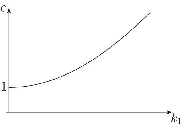
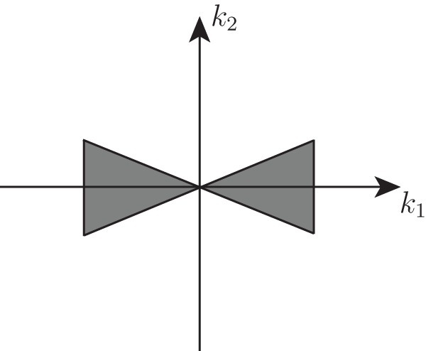


 Open access