


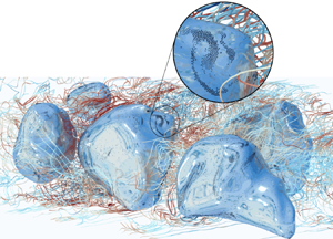



1. Introduction
The process of particle capture and subsequent trapping on the surface of deformable drops in turbulence may have important consequences on surface properties. At the microscale, particles are expected to act in a way similar to soluble surfactant molecules, affecting surface tension in particular (Binks Reference Binks2002; Soligo, Roccon & Soldati Reference Soligo, Roccon and Soldati2019b; Wang & Brito-Parada Reference Wang and Brito-Parada2021). This has important consequences at the macroscale, influencing drop deformability and hence coalescence and breakup processes. While the effect of soluble surfactants on local modifications of the surface tension has been widely investigated (Stone & Leal Reference Stone and Leal2006; Bzdek et al. Reference Bzdek, Reid, Malila and Prisle2020; Manikantan & Squires Reference Manikantan and Squires2020; Soligo, Roccon & Soldati Reference Soligo, Roccon and Soldati2020), the effect of particles has received comparatively little attention, in particular as far as particle loading and spatial distribution at the interface are concerned (Gu & Botto Reference Gu and Botto2016, Reference Gu and Botto2020).
Most of the available studies focus on heterogeneous mixtures of suspended colloidal particles, in which the flow conditions are dominated by viscous forces (Liu et al. Reference Liu, Bigazzi, Sharifi-Mood, Yao and Stebe2017; Davis & Zinchenko Reference Davis and Zinchenko2018; Liu et al. Reference Liu, Zhang, Ba, Wang and Wu2020; Roure & Davis Reference Roure and Davis2021). Examples include foam and emulsion stabilization problems, where particles are adsorbed at an air–water interface and are found to increase the surface dilational elasticity (Wang & Brito-Parada Reference Wang and Brito-Parada2021). Stabilization is achieved by assembling the particles into organized structures on the interface. The assembly is typically directed by external guiding fields that control the capillary interactions among the adsorbed particles (Liu et al. Reference Liu, Bigazzi, Sharifi-Mood, Yao and Stebe2017; Liu, Sharifi-Mood & Stebe Reference Liu, Sharifi-Mood and Stebe2018). One such field is the interface curvature: particles move along curvature gradients and form structures that are related to these gradients (Liu et al. Reference Liu, Bigazzi, Sharifi-Mood, Yao and Stebe2017).
In many industrial and environmental applications, however, a key factor is represented by turbulence. The interaction between small solid particles and fluid interfaces under the action of an underlying turbulent flow is crucial, for instance, in scavenging by raindrops or in scrubbing processes, where the overall abatement efficiency depends on the ability of a drop to trap particles for very long times (Wang, Song & Yao Reference Wang, Song and Yao2016). Other examples include three-phase gas–liquid–solid mixtures in which bubbles rise through slurries and particles may be inserted to enhance mass transfer, such as in the Fischer–Tropsch process where particles are metal catalysts (Chen et al. Reference Chen, Wei, Duyar, Ordomsky, Khodakov and Liu2021) or mineral processes where bubbles are used to capture hydrophobic particles and float them out of a slurry (Ojima, Hayashi & Tomiyama Reference Ojima, Hayashi and Tomiyama2014).
Up to now, a detailed physical understanding of particle–interface interactions under turbulent conditions is missing. A primary reason is the wide range of length scales involved, from the particle microscale to the drop mesoscale (Pozzetti & Peters Reference Pozzetti and Peters2018; Elghobashi Reference Elghobashi2019; De Vita et al. Reference De Vita, Rosti, Caserta and Brandt2019). This scale separation makes it hard to establish a clear link between particle attachment, surface tension and drop deformability, either experimentally or numerically (Soligo et al. Reference Soligo, Roccon and Soldati2019b). The present paper represents a first step towards the establishment of such a link by proposing a novel combination of computational models to examine the complex dynamics produced by a moving, deformable interface covered by very small particles in a turbulent system accounting for the multiscale nature of the process. We are only aware of one other study, by Zeng et al. (Reference Zeng, Velez, Lu and Tryggvason2021), in which a similar particle-laden, three-phase turbulent flow configuration is examined. The study uses a front tracking/finite volume method to perform direct numerical simulations of large swarms of bubbles and drops, while the particles are modelled as very viscous drops that are kept spherical by imposing a very high surface tension.
The presence of a compliant interface is crucial as it modulates the overall energy and momentum transfer between the carrier fluid and the drops (Soligo et al. Reference Soligo, Roccon and Soldati2020), but also controls the efficiency with which particles are removed from the fluid. We investigated recently the process of particle removal by deformable drops (Hajisharifi, Marchioli & Soldati Reference Hajisharifi, Marchioli and Soldati2021), showing that particles are transported towards the interface by jet-like turbulent motions and, once close enough, are captured by interfacial forces in regions of local flow expansion characterized by positive velocity divergence. On the other hand, fluid motions characterized by high strain and high dissipation are generally avoided by the particles. In the present paper, we build on this knowledge to examine particle dynamics during the trapping stage, when particles interact with the drop surface. In particular, we focus our attention on the preferential distribution of the particles and its correlation with the interface topology. To this aim, we rely on original simulations in which excluded-volume effects (EVE) are accounted for by enforcing interparticle collisions.
In the three-phase flow configuration that we examine, collisions occur almost exclusively between trapped particles, namely on a two-dimensional deformable surface. This implies that the excluded volume is associated with the surface itself, and provides a way to impose a no interpenetration constraint to the particles. While computationally expensive, EVE allow us to explore the evolution of patterns that stem from the interaction of sub-Kolmogorov, quasi-inertialess spherical particles with super-Kolmogorov drops. These patterns are more realistic than those resulting from non-colliding point particles that are allowed to overlap. We are able to show that particle spatial distribution correlates with specific interface topologies, which we characterize via the divergence of the velocity field on the surface. We also correlate particle clusters with the local interface curvature, in view of the potential modulation that trapped particles may produce on the surface tension and, hence, on the drop deformability.
2. Three-phase flow modelling
We consider a turbulent Poiseuille flow in a channel, performing direct numerical simulations of the Navier–Stokes equations, coupled with a phase-field method to describe the dynamics of the drop surface and a Lagrangian approach to compute particle trajectories.
2.1. Coupling of interface dynamics and hydrodynamics
The phase-field method describes the transport of the phase indicator  $\phi$, providing the instantaneous shape and position of the interface: $\phi$ is constant in the bulk of both the carrier phase ( $\phi = - 1 \equiv \phi _-$) and the drops ( $\phi = + 1 \equiv \phi _+$), while undergoing a smooth transition across an interface-centred layer of dimensional thickness $\xi$. The position of the interface is given by the $\phi = 0$ isolevel. The evolution of $\phi$ is given by the Cahn–Hilliard equation, which can be made dimensionless using the friction velocity $u_{\tau }=\sqrt {\tau _w/\rho _f}$, with $\tau _w$ the mean wall shear stress, and the maximum positive value of the order parameter, $\phi _+$. In this form, the equation reads as
 \begin{equation} \frac{\partial \phi}{\partial t}+{\boldsymbol{u}}\boldsymbol{\cdot}\boldsymbol{\nabla}\phi=\frac{1}{Pe_{\phi}}\nabla^2 \mu_{\phi} + f_p, \end{equation}
where  ${\boldsymbol {u}}=(u,v,w)$ is the fluid velocity vector, $Pe_{\phi }$ is the Péclet number, $\mu _{\phi }$ is the chemical potential and $f_p$ is a penalty flux introduced to force the interface towards its equilibrium by reducing the diffusive fluxes induced by $\mu _{\phi }$ (Soligo, Roccon & Soldati Reference Soligo, Roccon and Soldati2019a). The Péclet number is defined as
 \begin{equation} Pe_{\phi}=\frac{u_{\tau} h}{M}, \end{equation}
with  $M$ the fluid mobility inside the order parameter transition layer and $h$ the half-height of the channel. This number represents the ratio between the diffusive time scale $h^2/M$ and the convective time scale $h/u_{\tau}h$ in the transition layer, and is the parameter that controls the interface characteristic relaxation time. The chemical potential is defined as the variational derivative of the Ginzburg–Landau free energy functional, $\mathcal {F}[\phi, \boldsymbol {\nabla } \phi ]$. In dimensionless form:
 \begin{equation} \mu_{\phi}= \frac{ \delta \mathcal{F}[\phi, \boldsymbol{\nabla} \phi]}{\delta \phi}=\phi^3 - \phi - Ch ^2 \nabla ^2 \phi, \end{equation}
whereas the penalty flux is defined as
 \begin{equation} f_p=\frac{\lambda}{Pe_{\phi}} \left[\nabla^2\phi - \frac{1}{\sqrt{2} Ch} \boldsymbol{\nabla} \boldsymbol{\cdot} \left((1-\phi^2) \frac{\boldsymbol{\nabla} \phi}{|\boldsymbol{\nabla}\phi|} \right) \right], \end{equation}
where  $\lambda$ is a parameter set according to the scaling proposed by Soligo et al. (Reference Soligo, Roccon and Soldati2019a) and $Ch=\xi / h$ is the Cahn number. When the system is at equilibrium, $\mu _{\phi }$ is uniform over the entire domain. The equilibrium profile for a flat interface located at $s=0$, $s$ being the coordinate normal to the interface, can be obtained by solving $\boldsymbol {\nabla } \mu _{\phi } =0$, which yields $\phi _{eq} (s)= \tanh ( s / \sqrt {2} Ch )$. For additional details, we refer the reader to Soligo et al. (Reference Soligo, Roccon and Soldati2019a), Soligo et al. (Reference Soligo, Roccon and Soldati2019b) and Soligo, Roccon & Soldati (Reference Soligo, Roccon and Soldati2021) and references therein.
The flow hydrodynamics is described by the continuity and Navier–Stokes equations, which are coupled with the Cahn–Hilliard equation. Following Hajisharifi et al. (Reference Hajisharifi, Marchioli and Soldati2021), we assume that the carrier fluid and the drops have the same density and viscosity. The corresponding dimensionless equations for these two phases read as
 \begin{equation} \boldsymbol{\nabla} \boldsymbol{\cdot} {\boldsymbol u} = 0,\quad \frac{\partial {\boldsymbol u}}{\partial t}+{\boldsymbol u} \boldsymbol{\cdot} \boldsymbol{\nabla} {\boldsymbol u}={-}\boldsymbol{\nabla} p+\frac{1}{Re_\tau}\nabla^2 {\boldsymbol u}+\frac{Ch}{We}\frac{3}{\sqrt{8}}\boldsymbol{\nabla} \boldsymbol{\cdot}\tau_c, \end{equation}
where  $\boldsymbol {\nabla } p$ is the sum of the mean pressure gradient that drives the flow and its fluctuating part; $Re_{\tau }= u_{\tau } h / \nu _f$ is the friction Reynolds number, with $\nu _f$ the fluid kinematic viscosity; $We=\rho _f u_{\tau }^2 h / \sigma$ is the Weber number, based on the surface tension $\sigma$ of a clean interface; and $\tau _c=|\boldsymbol {\nabla } \phi |^2 I - \boldsymbol {\nabla } \phi \otimes \boldsymbol {\nabla } \phi$ is the Korteweg stress tensor, which accounts for the interfacial force induced on the flow by the occurrence of capillary phenomena.
2.2. Lagrangian tracking and particle–interface interaction model
Particles are assumed to be neutrally buoyant and smaller than the Kolmogorov length scale in size. They are subject to two force contributions: the drag force and the capillary force that acts only when the particles interact with the interface, thus allowing for particle adhesion. The capillary force represents the force exerted on a spherical particle embedded in a fluid interface and results from the surface tension acting at the three-phase contact line. When an adsorbed spherical particle is being displaced perpendicularly from a fluid interface, this force increases as the liquid bridge extending from the particle surface to the plane of the undisturbed fluid interface becomes curved (Gu & Botto Reference Gu and Botto2016, Reference Gu and Botto2020). The resulting equations of particle motion, in dimensionless vector form, read as
 \begin{equation} \frac{\partial {\boldsymbol{x}}_p}{\partial t}={\boldsymbol{u}}_p,\quad \frac{\partial {\boldsymbol{u}}_p}{\partial t}=\frac{{\boldsymbol{u}}_{@p}-{\boldsymbol{u}}_p}{St}+\frac{6{\mathcal{A}}}{\rho_p /\rho_f} \frac{Re_{\tau}}{We} \frac{{\mathcal{D}}}{{d_p}^{3}} {\boldsymbol{n}}, \end{equation}
where the last term on the right-hand side represents the capillary force. In (2.6),  ${\boldsymbol {x}}_p$ and ${\boldsymbol {u}}_p$ are the dimensionless particle position and velocity, respectively; ${\boldsymbol {u}}_{@p}$ is the dimensionless fluid velocity at particle position (obtained using a fourth-order Lagrange polynomials interpolation scheme); $St=\tau _p/\tau _f$ is the Stokes number, the ratio of the particle relaxation time $\tau _p=\rho _p d_p^2/18 \mu _f$ (with $d_p$ the particle diameter and $\mu _f$ the fluid dynamic viscosity) to the carrier fluid characteristic time $\tau _f=\nu _f /{u_{\tau }}^2$; ${\mathcal {A}}$ is a dimensionless parameter that incorporates the effect of the contact angle between the particle and the interface, as well as the effect of the particle-to-drop-size ratio; and ${\mathcal {D}}$ is the interaction distance between the centre of the particle and the nearest $\phi =0$ point, which defines the range of action of the capillary force: this force acts only when ${\mathcal {D}} \le d_p/2$ and is activated after a particle coming from either phase crosses the interface for the first time. Note that the value of ${\mathcal {D}}$ may change as the particle moves relative to the interface. Finally, ${\boldsymbol n}$ is the normal unit vector pointing from the particle centre to the $\phi =0$ isolevel. We remark here that particles are always in the Stokes regime, since their Reynolds number $Re_{p}=|{\boldsymbol {u}}_{@p}-{\boldsymbol {u}}_p|d_p / \nu _f$ was verified to be always significantly smaller than unity throughout the simulations. The expression of the capillary force is valid for small spherical particles adsorbed at a fluid interface (Ettelaie & Lishchuk Reference Ettelaie and Lishchuk2015; Gu & Botto Reference Gu and Botto2020), and corresponds to the case in which particle wettability leads to entrapment at the interface (no sinking, no rebound) (Chen et al. Reference Chen, Liu, Lu and Ding2018). The value of ${\mathcal {A}}$ satisfies the condition that the adsorption energy balances the desorption energy required for particle detachment from the interface (Ettelaie & Lishchuk Reference Ettelaie and Lishchuk2015): for a contact angle equal to $90^{\circ }$, as assumed in the present simulations, one gets ${\mathcal {A}}=2$. Additional runs were also performed to assess the effect of a change in the value of ${\mathcal {A}}$, and hence in the magnitude of the capillary force, on particle dynamics. As far as the statistical quantities discussed in § 3 are concerned, no major effect was observed (small quantitative modifications).
The spatial distribution of the capillary force across the transition layer centred at the drop interface is shown in figure 1, together with the spatial distribution of the order parameter. In general, the capillary force depends on the contact angle and on the filling angle (namely the angle formed between the unperturbed fluid interface and the line connecting the particle centre to the contact line). More details can be found in Gu & Botto (Reference Gu and Botto2020). In our simulations, information on the values of these two angles is not available because the boundary conditions at the particle surface are not enforced explicitly, and the fluid interface is resolved also inside the volume occupied by the particle, which is assumed to be pointwise. In spite of these limitations, it is still possible to model the capillary force in the limit of small distortion of the fluid interface, for which the capillary force is a linear function of the interface distortion itself. When the interface distortion becomes larger than a threshold value, which corresponds to the threshold value for  ${\mathcal {D}}$, it is assumed that the particle can be removed from the interface and, therefore, that the capillary force is no longer exerted on the particle. Note that, in principle, a particle can escape from the potential well associated with the capillary force (e.g. under the action of strong enough turbulent fluctuations in the proximity of the drop surface). In our simulations, we observed such an event only rarely.
Spatial distribution of the order parameter and capillary force. The order parameter  $\phi$ transitions from $-1$ (corresponding to the carrier fluid) to $+1$ (corresponding to the drop) across a layer of thickness $\mathcal {T} = 4.1 Ch$. The capillary force, labelled as $F_c$ in this figure, is zero everywhere except within a distance ${\mathcal {D}}$ from the interface, where its absolute value decreases linearly with the separation between the particle centre and the interface. In this work, ${\mathcal {D}}=d_p/2$ and ${\mathcal {D}} / \mathcal {T}\simeq {{O}}(10^{-1})$.

2.3. Modelling and importance of EVE
Excluded-volume effects are modelled through interparticle collisions. The proactive collision algorithm proposed by Sundaram & Collins (Reference Sundaram and Collins1996) is used. Collisions are detected at the beginning of each time step through the explicit calculation of the collision time  $t_{ij}$ for the $i$th and $j$th particles, and then enacting the collision whenever $0 \le t_{ij} \le \Delta t$ (Sundaram & Collins Reference Sundaram and Collins1996). Particles are advanced in time over the subinterval $t_{ij}$ and then the algorithm searches for new collisions, thus allowing for multiple collisions of the same particle. We considered hard-sphere elastic collisions that are momentum and energy conserving: this way, collisions play no role in the total particle kinetic energy since the total kinetic energy of the colliding pair is conserved. To reduce the computational cost of identifying the colliding pairs, we adopted the strategy of subdividing the computational domain into smaller ‘neighbourhoods’, within which potential partners for collision are selected. Minimizing the computational effort of collision detection is crucial, considering that collisions occur almost exclusively between trapped particles (as already mentioned, particles are almost inertialess and tend to follow the flow pathlines neatly as long as they remain in the carrier fluid domain) and that the number of trapped particles increases significantly in time. Because we consider pointwise particles, we can only model collisions since they must be treated at a subgrid level and we cannot resolve explicitly for the hydrodynamic interactions between colliding particles as can be done in particle-resolved simulations (Kempe & Fröhlich Reference Kempe and Fröhlich2012; Brandle de Motta et al. Reference Brandle de Motta, Breugem, Gazanion, Estivalezes, Vincent and Climent2013; Uhlmann & Chouippe Reference Uhlmann and Chouippe2017; Costa, Brandt & Picano Reference Costa, Brandt and Picano2020, Reference Costa, Brandt and Picano2021). However, we are not specifically interested in characterizing collisions (e.g. in terms of energy dissipation or collision rates). The reason is that, in the present three-phase flow, collisions occur almost exclusively between trapped particles and therefore involve small amounts of particle kinetic energy and momentum exchanged, as well as negligible energy dissipation. Rather, we exploit collisions to ensure a more physical representation of particle distribution of the drop surface. This feature is of great importance for the accurate modelling of the surface tension modifications induced by the particles: it prevents the occurrence of concentration peaks that are unphysically high, which would lead to overestimated surface tension changes in some regions of the interface, while producing underestimated changes in regions depleted of particles. Note that, for the present problem, particle collisions in the bulk of the carrier fluid are negligible and therefore the computational cost of the collision algorithm is ${{O}} (N_t \log N_t )$, with $N_t$ the number of particles trapped on the drop surface. In addition, the collision frequency scales with the local volumetric concentration of the particles, here inversely proportional to the surface area covered by the particles times the particle diameter. Such concentration is much higher than the concentration one would typically find in a dropless flow at the same volume fraction. As a result, the collision algorithm becomes increasingly expensive as the simulation time increases, amounting up to approximately $80\,\%$ of the computational cost of one time step.
The effect of lubrication forces was not included in the simulations. The reason for this choice is the following. A common approach would be to describe the interaction forces between particles in a suspension by the DLVO theory (Israelachvili Reference Israelachvili2011). The DLVO force is regarded as the sum of an attractive van der Waals force and a repulsive electric double layer force. Other non-DLVO forces exist when two particles are in close range such as the hydration force and the steric force (Liang et al. Reference Liang, Hilal, Langston and Starov2007). Modelling these forces, however, requires knowledge of the material properties of the particles and the surrounding liquid solutions, as well as other physical–chemical parameters. In addition, as suggested by Tsuji, Kawaguchi & Tanaka (Reference Tsuji, Kawaguchi and Tanaka1993) and by Mikami, Kamiya & Horio (Reference Mikami, Kamiya and Horio1998) for discrete particle simulations, details of the particle–particle interaction model should not significantly affect the collective behaviour of the particles as long as the collisions between particles are regular enough. This is the case for the (mono)layer formed by the trapped particles, since each particle is constantly interacting with neighbouring particles. For the current version of the particle tracking model, we thus decided to limit particle–particle interaction to collisions. An alternative option, which we are currently examining, would be to adopt a generic linear repulsive force law, as proposed by Gu & Botto (Reference Gu and Botto2020). This force, which is essentially a relaxed version of the hard-sphere contact force, could represent a computationally viable alternative to explore the effect of interparticle repulsion on the mechanical properties of a particle-laden interface, which is the main future development of the present work.
2.4. Numerical method and simulation set-up
The governing equations (2.1) and (2.5) are solved numerically using a pseudo-spectral method that transforms the field variables into wave space using Fourier series in the homogeneous directions (streamwise  $x$ and spanwise $y$), and Chebychev polynomials in the wall-normal direction, $z$. The Helmholtz-type equations so obtained are advanced in time using an implicit Crank–Nicolson scheme for the linear diffusive terms and an explicit two-step Adams–Bashforth scheme for the nonlinear terms. The Cahn–Hilliard equation is discretized using an implicit Euler scheme (Badalassi, Ceniceros & Banerjee Reference Badalassi, Ceniceros and Banerjee2003; Yue et al. Reference Yue, Feng, Liu and Shen2004). All unknowns (velocity and phase field) are Eulerian fields defined on the same Cartesian grid, which is uniformly spaced in $x$ and $y$ and suitably refined close to the wall along $z$ by means of Chebychev–Gauss–Lobatto points. Periodicity is imposed on all variables in $x$ and $y$, whereas a no-slip condition is enforced at the two walls. Interphase mass leakage is minimized (below $5\,\%$ of the initial drop volume) using a flux-corrected formulation (Soligo et al. Reference Soligo, Roccon and Soldati2019b), and occurs only prior to particle injection, namely before the surface area of the drops has reached a steady state. As far as the Lagrangian tracking is concerned, the particle motion equations given by (2.6) are advanced in time using an explicit Euler scheme and the same time step of the fluid, $\delta t = \tau _p / 10$. Particles are randomly injected within the volume occupied by the carrier fluid with initial velocity ${\boldsymbol u}_p (t_{tr}=0)={\boldsymbol u}_{@p} (t_{tr}=0)$, with $t_{tr}$ the particle tracking time. More details can be found in Hajisharifi et al. (Reference Hajisharifi, Marchioli and Soldati2021).
The simulation parameters are reported in table 1. The values of  $Re_{\tau }$, $We$ and $St$ match those considered by Hajisharifi et al. (Reference Hajisharifi, Marchioli and Soldati2021) and correspond to the case of low-viscosity silicone oil drops and very small colloidal particles in water. The effect of the Reynolds number was assessed by Soligo et al. (Reference Soligo, Roccon and Soldati2020), who showed negligible modifications of the statistical properties of the droplet-laden turbulence up to $Re_{\tau }=300$. The effect of the Weber number was assessed here up to $We=1.5$, and appears to also produce minor quantitative modifications of the statistics. The grid spacings and the range of variation of the Kolmogorov scales are expressed in wall units, identified by the superscript + hereinafter, and obtained using $u_{\tau }$ as reference velocity, $\nu _f/u_{\tau }$ as reference length and $\nu _f / u_{\tau }^2$ as reference time. The choice of the grid resolution (see table 1) was determined by a compromise between the best possible accuracy of the simulations and the computational cost. The effect of the grid resolution on the behaviour of the statistical observables examined in § 3 is discussed in Appendix A.
Summary of simulation parameters. Cases with and without EVE are reported in the last row of the table. Results discussed in § 3 refer to the simulations highlighted in grey. Superscript + indicates variables in wall units, obtained using  $u_{\tau }$ as reference velocity, $\nu _f/u_{\tau }$ as reference length and $\nu _f / u_{\tau }^2$ as reference time. Note that the grid spacings provide an extremely well-resolved turbulent flow field compared to the single-phase case. The entire simulation campaign required nearly 15M CPU-hours on a large-scale parallel Tier-0 infrastructure with a raw data production of approximately 20 TB.

For the phase field, the value  $Ch=0.02$ allowed us to accommodate at least five grid points across the order parameter transition layer (Soligo et al. Reference Soligo, Roccon and Soldati2019a, Reference Soligo, Roccon and Soldati2020). This corresponds to a thickness of approximately 14.8 wall units, which is four to nine times the Kolmogorov length scale in the flow simulated here. We remark here that the Cahn number (which is the dimensionless thickness of the transition layer) scales with the grid resolution in all three directions. Therefore halving the Cahn number, namely halving the thickness $\xi$ with respect to the channel half-height $h$, would make the computational cost of the simulation eight times larger, quickly making the simulations extremely expensive (especially those with EVE). However, it should also be considered that the Korteweg stresses scale with $\boldsymbol {\nabla } \phi$, and this quantity is significantly larger in the central nodes of the stencil used to sample the transition layer, while becoming nearly negligible at the end nodes. This implies that the Korteweg stresses, and hence the surface tension, are mostly affecting the fluid momentum equations within a limited portion of the transition layer (a sort of ‘effective’ thickness), typically confined within two or three grid points. In our simulations, this portion is approximately seven wall units, corresponding to roughly two grid cells. It should be also considered that the droplets tend to occupy the central region of the flow, where the local Kolmogorov length scale is larger, and avoid the near-wall region, where local Kolmogorov length scale is smaller. Therefore, while it is true that even the effective transition layer thickness is larger than the Kolmogorov scale, it is also true that the ratio of these two quantities is reasonably small.
We remark here that the extent of the transition layer does not represent the physical thickness of the interface, which is identified solely by the ensemble of points in the computational domain where  $\phi =0$. The minimum number of grid points required to describe the order parameter transition from one fluid to the other is determined by the need to provide an accurate description of the steep gradients at the interface, while ensuring that the so-called sharp-interface limit (i.e. the small-thickness asymptotic state where the system evolution becomes independent of the effective parameters) is met Magaletti et al. (Reference Magaletti, Picano, Chinappi, Marino and Casciola2013). To achieve this limit, it is necessary to provide the correct relationship between the transition layer thickness and the interface mobility $M$, namely the relationship that allows recovery of the correct physical properties of the interface. In our simulations, we adopted the relationship suggested by Magaletti et al. (Reference Magaletti, Picano, Chinappi, Marino and Casciola2013), who showed that a scaling of the form $M \propto Ch^2$ is the only correct procedure to approach the limit of vanishing Cahn number while retaining the known dynamics of a sharp interface between immiscible fluids. More specifically, Magaletti et al. (Reference Magaletti, Picano, Chinappi, Marino and Casciola2013) demonstrated that, through this scaling, it is possible to asymptotically guide the solution of the diffuse interface model towards the same sharp interface behaviour observed in the experiments in the limit of vanishing interface thickness. The physical interpretation of this result is that the mobility should suitably change as the interface thickness keeps on reducing, in order to maintain the effective interface force consistent with the required surface tension. In the present study, the scaling yields $Pe_{\phi }=1/Ch=50$. Note that, as shown by Soligo et al. (Reference Soligo, Roccon and Soldati2019b), a reduction of the transition layer thickness operated within the sharp-interface limit may have a quantitative effect on the final number of droplets, yet not on their size distribution and total steady-state surface area. The phase field was initialized to generate a regular array of $N_{d,0}=256$ spherical drops with normalized diameter $d/h=0.4$ (corresponding to $d^+=60$ in wall units) that are injected in a fully developed turbulent flow. Memory of the initial condition chosen for the drops is completely lost after a short transient and the analysis performed at statistically steady state is not affected by the imposed initial condition. Different initial conditions have been tested, for instance, the injection of a thin liquid sheet at the channel centre, and the same statistically steady-state results were obtained. In addition, the selected initial condition has a shorter transient before reaching statistically steady-state results with respect to the other configurations tested. Thus, to reduce the computational cost of the simulations and to better compare the obtained results with those of Hajisharifi et al. (Reference Hajisharifi, Marchioli and Soldati2021), the present initial condition for the dispersed phase has been used. After initialization, drops undergo both breakup and coalescence, and the drop size distribution varies with respect to the initial one. For the range of flow parameters considered in our study, coalescence events are predominant over breakup events and the net effect is to reduce significantly the number of drops in time, $N_d/N_{d,0}$, shown in figure 2, as well as the total drop surface area, $A_d/A_{d,0}$, shown in the inset of figure 2. Clearly, a corresponding increase of the mean drop size is observed. The inset in figure 2 shows that the total drop surface reaches a statistically steady state when the surface area of all the remaining drops has become roughly one-third of its initial value. Once this steady state is reached, particles are finally injected into the volume occupied by the carrier fluid. The injection time is indicated by the vertical lines in figure 2. At this time, we count 12 drops, which are visualized in figure 3 together with the particles (note that only one-third of the injected particles and only particles in the bottom half of the domain are shown for ease of visualization) and the streamwise fluid velocity distribution close to the channel wall.
Time evolution of the number of drops,  $N_d/N_{d,0}$ (main panel), and of the total surface area of the drops, $A_d/A_{d,0}$ (inset). The vertical dashed lines indicate the time at which particles are injected into the carrier fluid domain and Lagrangian tracking starts. The thin horizontal line in the inset indicates the steady-state value of the total surface area of the drops.

Snapshot of the drop distribution inside the computational domain at the time of particle injection (as indicated in figure 2). Particles are rendered as black dots, whereas the bottom boundary of the domain is coloured by the streamwise carrier fluid velocity. For visualization purposes, only one particle out of three and only those located in the bottom half of the domain are shown.

The drops shown in figure 3 have an average sphere-equivalent diameter of approximately  $150$ wall units, with a minimum value equal to approximately $50$ wall units and a maximum value of approximately $200$ wall units. These values are given here to provide an indication of how broad the size distribution becomes, but also to demonstrate that, because of the increased mean drop size, the drop-to-particle-size ratio is ${{O}} (10^2)$ or larger when particles are injected into the flow. Considering the significant modification that the drop distribution undergoes in time, the selection of the particle injection time was aimed at removing as much as possible the influence that variations of the mean drop size and total drop surface might have on the particle capture and trapping processes.
Two sets of  $N_p=5 \times 10^5$ particles were tracked, with an initial particle-to-drop-diameter ratio $d_p / d \simeq {{O}} (10^{-2})$ within the range of $St$ examined. Note that different sets of particles were considered to examine possible effects due to a slight change of particle inertia on the particle capture rates and on the subsequent formation of particle patterns on the surface of the drops. The particle diameter in wall units, $d_p^+= d_p / ( \nu _f / u_{\tau } )$, can be expressed directly as a function of the Stokes number: $d_p^+=\sqrt {18 \, St}$. This yields $d_p^+ \simeq 1.3$ for the $St=0.1$ particles and $d_p^+ \simeq 3.8$ for the $St=0.8$ particles. The diameter for the $St=0.1$ particles is smaller than the Kolmogorov length scale everywhere in the flow domain, whereas the diameter for the $St=0.8$ particles is comparable to the local value of the Kolmogorov length scale in the centre of the channel (while being approximately two times larger than this scale near the wall). However, in the present study, we are interested in the dynamics of particles that are trapped at the drop interface rather than those interacting with the carrier flow turbulence. Hence, we believe that the marginal effect of particle inertia that we observe is just weakly affected by particle interaction with the small-scale structures of the flow (but, rather, depends on the interaction of the particles with the interface flow topologies). In terms of the particle volume fraction, defined as $\phi _V = N_p V_p^+ / V_f^+$ with $V_p^+$ the particle volume in wall units and $V_f^+$ the volume occupied by the fluid and the drops, the diameters we considered yield $\phi _V \simeq 3.8 \times 10^{-4}$ for the $St=0.1$ particles and $\phi _V \simeq 8.6 \times 10^{-3}$ for the $St=0.8$ particles. The particle response time $\tau _p$ can also be related directly to the Stokes number as follows: $\tau _p = St \cdot \tau _f$. Since the time step size is $\delta t = \tau _p /10$, one obtains $\delta t = St \cdot \tau _f / 10$. Hence, for the $St=0.1$ particles ( $St=0.8$ particles) the ratio of the time step size to the frictional time scale is $\delta t / \tau _f = 10^{-2}$ ( $\delta t / \tau _f = 8 \times 10^{-2}$).
A final comment about the feedback of the particles on the carrier fluid and on the drops is in order. This feedback is associated with the force exerted by the particles per unit volume of fluid,  $\varOmega ^+$. In our problem, this force can be expressed in dimensionless form as
 \begin{equation} {\boldsymbol f}_{2W,K}^+{=} \sum_{p=1}^{n_p} \left[ - 3 {\rm \pi}({\boldsymbol u}^+_{@p} - {\boldsymbol u}^+_p ) d_p^+ N_K \left( {\boldsymbol x}^+_p \right) / \varOmega^+ \right], \end{equation}
where subscript  $K$ indicates the grid node onto which the force is redistributed, $n_p$ is the number of particles contributing to ${\boldsymbol f}_{2W,K}^+$ and $N_K$ is the shape function adopted for the redistribution onto the $K$th node of the force exerted by the fluid on the $p$th particle (the drag force, in our simulations). Note that the shape function depends on the position ${\boldsymbol x}_p^+$ of the particle. As long as the particles are transported by the carrier fluid, the feedback force ${\boldsymbol f}_{2W,K}^+$ can be safely neglected because of the low inertia of the particles, which tend to follow almost perfectly the fluid motions (and hence rarely collide). Clearly, collisions play a role once particles remain trapped at the interface, as is discussed in the next section. Another important factor to be considered is the rather low average particle volume fraction observed within the carrier fluid. Particles do not exhibit a strong tendency to preferentially concentrate into clusters before being captured at the interface (Hajisharifi et al. Reference Hajisharifi, Marchioli and Soldati2021): this behaviour keeps the particle volume fraction low also locally, limiting the value of $n_p$ in (2.7) and allowing us to neglect particle feedback on the flow field.
The two-way coupling effects by the trapped particles can also be neglected, in view of the particle-to-fluid density ratio (equal to unity) and the small particle inertia, determined by the combination of a rather low density ratio and a small particle diameter. Because of these two factors, the relative velocity between the particles and the surrounding fluid is always much smaller than unity, as we verified by looking at the particle Reynolds number,  $Re_p = | {\boldsymbol u}^+_{@p} - {\boldsymbol u}^+_p | d_p^+$ (Hajisharifi et al. Reference Hajisharifi, Marchioli and Soldati2021). Since ${\boldsymbol f}_{2W,K}^+ \propto Re_p$, the two-way coupling term turns out to be about two to three orders of magnitude smaller than the other terms in the Navier–Stokes equations, for the present simulations. The minor role attributed to two-way coupling effects is supported also by several literature studies in which one-way coupled simulations of small neutrally buoyant particles in isotropic homogeneous turbulence showed excellent agreement with measurements (Volk et al. Reference Volk, Calzavarini, Verhille, Lohse, Mordant, Pinton and Toschi2008), and non-negligible turbulence modulations are typically found only for finite-size, neutrally buoyant particles, as shown by Wang & Richter (Reference Wang and Richter2019) and Brandle de Motta et al. (Reference Brandle de Motta, Estivalezes, Climent and Vincent2016) among others.
3. Results and discussion
In this section, we examine first the impact of EVE on the overall particle trapping rate. A particle is counted as trapped if the following three criteria are met: (1) the particle must first cross or land on the  $\phi =0$ surface, which identifies the interface, coming from the carrier fluid; (2) the particle has to remain confined in a region of the flow where $\phi =0 \pm \delta \phi$, with $\delta \phi$ equal to the value of the phase indicator at a distance $d_p/2$ from the interface; and (3) the particle must sample this region for a minimum time window $\Delta t$, chosen to be a multiple of the volume-averaged value of the Kolmogorov time scale.
The first criterion is obvious, considering that particles are initially released inside the carrier fluid domain only. The second criterion allows us to isolate those particles that touch the interface, upon having crossed it or having landed on it. The effect of turbulence is such that particles may want to escape from the interface: as a result, particles may not sample the  $\phi =0$ iso-surface exactly, albeit being still trapped. In order to escape from the interface, particles must be able to overcome the effect of the capillary force, which acts up to a distance $d_p/2$ from the interface, where the phase indicator has the value $\delta \phi$. The third criterion is meant to exclude situations in which the particle is able to cross the interface without being trapped: this may happen if the particle is able to overcome the effect of the capillary force right after having crossed the interface. The time window $\Delta t$ is chosen to be sufficiently larger than the average time taken by a particle to cross the transition layer, which was shown to scale with the volume-averaged Kolmogorov time scale, $\langle \tau _K \rangle$ (Hajisharifi et al. Reference Hajisharifi, Marchioli and Soldati2021). Considering dimensionless quantities, we have thus defined $\Delta t^+ = N \cdot \langle \tau _K^+ \rangle$ and made several calculations at varying $N$, in order to assess the effect of the time window length on the statistics (trapping rate, in particular). The maximum time window we considered was $\Delta t^+ = 3 \langle \tau _K^+ \rangle \simeq 30$ in wall units. We found minimal dependence of the statistics on $\Delta t^+$, namely on $N$, since nearly all of the particles remain trapped after the first interface crossing/landing event and, therefore, the third criterion is very rarely applied. In the process of counting the trapped particles, we use the interaction distance ${\mathcal {D}}$ to determine the local value of the phase indicator at the particle position, $\phi _{@p}$, that enters criterion (2) and must satisfy the condition $| \phi _{@p} | < \delta \phi$.
We then proceed by discussing the correlation between particle distribution and specific topological regions of the drop surface. Unless otherwise stated, we focus on the statistics for the  $St=0.1$ particles only. This because particle inertia was found to have predictable effects on the dynamics of trapped particles (limited to quantitative deviations in the statistics) within the range of $St$ considered in this study.
3.1. Excluded-volume effects on particle trapping rate
Physical intuition suggests that EVE play a marginal role in determining the particle dynamics as long as the particles, which are quasi-inertialess, are confined within the carrier fluid. In addition, since particle adhesion to the drop surface is controlled by specific carrier fluid motions, described in detail in Hajisharifi et al. (Reference Hajisharifi, Marchioli and Soldati2021), one might expect EVE to be of secondary importance for determining the rate at which particles are captured by the surface. When trapped particles are not allowed to overlap, however, the overall coverage of the drop surface will be higher than that predicted in the case of non-interacting particles and the resulting particle engulfment might prevent the occurrence of some capture events (a particle reaching the drop surface at a location already occupied by another particle will either bounce back into the carrier fluid domain or detach one or more particles). To quantify the actual impact of particle–particle interactions on the particle trapping rate, in figure 4 we show the time evolution of the number  $N_t$ of trapped particles, normalized by the total number of tracked particles $N_p$, with and without EVE (blue and red curve with symbols, respectively). The inset shows the area $A_p$ that is covered by the particles when EVE are considered. The area $A_p$ is determined considering the projected surface of the trapped particles, $A_{proj} = {\rm \pi}d_p^2 / 4$. Therefore, at a given time instant, $A_p(t)= N_t \times A_{proj}$. In computing $A_p$, we did not take into account maximum packing effects so $A_p$ provides a conservative measure of the covered interfacial surface. When trapped particles are arranged such that the densest packing condition is achieved, a portion of the interfacial surface (approximately 20 %) is not covered by the particles but cannot be occupied by other particles either. This portion could thus be considered as covered, since it cannot accommodate more trapped particles. However, it is rather complicated and time consuming to compute the actual particle packing in our simulations, and visual inspection suggests that very dense packing is achieved only where the largest clusters are formed. This has led to the choice of neglecting this contribution. Indeed, if all trapped particles satisfied the densest packing condition, then we would have found $A_p / A_d \simeq 18\,\%$ instead of $A_p / A_d \simeq 15\,\%$ at the end of the simulation.
Time evolution of the number of  $St=0.1$ particles trapped at the interface, $N_t$, normalized by the total number of particles, $N_p$. Symbols: $- \blacktriangle -$ (red), without EVE; $- \bullet -$ (blue), with EVE. The inset shows the increase in time of the interface area covered by the trapped particles, $A_p$, normalized by the total interface area of the drops, $A_d$.

In figure 4,  $A_p$ is normalized by the instantaneous total area of the drops, $A_d$: the ratio $A_p/A_d$ is equal to unity when the drop surface is entirely covered by the particles at maximum packing density. Time $t^+=0$ is the time at which the particles are injected into the flow. At this time, the time average of $A_d$ has reached a statistically steady value. However, as shown in the inset of figure 2, the instantaneous value of $A_d$ (which we used to compute the ratio) still fluctuates around the steady-state value. It can be observed that the number of trapped particles increases in time at a rate that is unaffected by particle interactions up to time $t^+ \simeq 1400$ from injection. Within this time window, the interface area covered by the particles remains relatively low (below $10\,\%$ of the total drop surface) and particle deposition appears to be controlled primarily by the turbulent fluctuations in the vicinity of the surface. At later times, the area coverage becomes large enough for deposition and trapping to be influenced also by particle interactions in the simulations with EVE. This effect adds to that produced by turbulence and leads to a lower number of trapped particles compared to the simulations without EVE: by the end of the simulation, approximately $46\,\%$ of the particles released into the flow have been trapped, instead of $50\,\%$. This is also reflected in the slower increase of $A_p/A_d$ visible in the inset of figure 4. The reduction of the trapping rate can be ascribed to two types of events: some particles are prevented from being captured in regions of the drop surface where the particle coverage has already reached the maximum packing limit (or is very close to it); some other particles may be displaced in the direction normal to the surface upon interacting with the nearby particles and thus find a way to escape from the interface (we remark here that this type of event is rarely detected in our simulations).
The effect on the evolution of  $N_t / N_p$ produced by a change in particle size, which may be expected to matter, is found to yield just quantitative modifications and is therefore discussed in Appendix B. In Hajisharifi et al. (Reference Hajisharifi, Marchioli and Soldati2021), we have shown that, if deposition is purely controlled by turbulent fluctuations, the time increase of $N_t/N_p$ can be predicted with very good accuracy using a simple model based on a single turbulent transport equation. This model exploits the similarity between the particle capture process and the process of particle deposition at a solid wall (Friedlander & Johnstone Reference Friedlander and Johnstone1957; Cleaver & Yates Reference Cleaver and Yates1975; Soldati & Andreussi Reference Soldati and Andreussi1996), and its only parameter scales with the turbulent kinetic energy of the fluid measured in the vicinity of the drop interface. The EVE-induced decrease in the number of trapped particles suggests that additional physics must be incorporated into the model, in order to account for the reduction of the surface area available for particle deposition and, hence, to provide an accurate prediction of the overall trapping efficiency. One possibility, which we are currently investigating, is to correct the predicted value of $N_t/N_p$ via a term that depends linearly on $A_p/A_d$.
3.2. Qualitative rendering of particle patterns and pattern morphology characterization
In figure 5, we show the instantaneous spatial distribution of the trapped particles at the final simulation time step (corresponding to time  $t^+ \simeq 3000$ from particle injection), when the particles have been trapped covering approximately $15\,\%$ of the total surface of the drops. For visualization purposes, only a portion of the entire computational domain is rendered: drops are coloured by the $\phi =0$ iso-surface, the flow field is rendered by the fluid streaklines and particles are visualized as small black dots. Two different situations are compared: particle distribution without and with EVE, shown in figures 5(a) and 5(b), respectively. In accordance with physical intuition, filamentary clusters characterized by high concentration of particles are observed when particles do not interact with each other and are allowed to overlap. On the other hand, particle distribution over the drop surface becomes more even when EVE are accounted for, as can be well appreciated from the two insets of figure 5. It is also apparent that, long after capture, particle clusters tend to form in the same portions of the interface. This observation implies that the dynamics of trapped particles is driven by flow phenomena that are unaffected by the interparticle interactions occurring in the accumulation regions of the interface. It also suggests that particle distribution may correlate with specific topological features of the interface.
Snapshot of particle distribution on the drop surface. Trapped particles form highly concentrated filamentary clusters without EVE (a), but appear more evenly distributed when EVE are accounted for (b).

To elaborate on these aspects, we examine the changes in the morphology of the clusters and characterize their correlation with the interface topology. We do so by using the correlation dimension, which can be used to measure the fractal dimension of the clusters. In its most general formulation, the correlation dimension is computed by choosing one base particle and counting the fraction  $n_p(r)$ of particles located within a sphere of radius $r$ surrounding the base particle. Any length-scale dependence of the statistics was removed by counting $n_p(r)$ for all possible values of $r$ to obtain the probability distribution of the distance between the base particle and the neighbouring particles. The procedure was then repeated for many randomly chosen base particles, averaging the results to obtain converged statistics. The correlation dimension is then obtained as (Grassberger & Procaccia Reference Grassberger and Procaccia1983)
 \begin{equation} D_{2} = \lim_{r \rightarrow 0} \frac{\ln \langle n_p(r) \rangle}{\ln r} \rightarrow \langle n_p(r) \rangle \sim r^{D_{2}}, \end{equation}
where  $\langle n_p(r) \rangle$ is the averaged, or expectation, value of $n_p (r)$. Based on (3.1), when particles are uniformly distributed over a surface (a line) around the base particle, $n_p(r)$ scales with $r^2$ ( $r$), so $D_{2} = 2$ ( $D_{2} = 1$). Since we are interested in clusters that form on the drop surface, we computed $\langle n_p(r) \rangle$ considering only the trapped particles and we refer to the correlation dimension as $D_{2@p}$ hereinafter. We remark here that conditioning the calculation of $D_{2}$ on the subset of trapped particles modifies significantly the statistics compared with the case in which all particles are considered: trapped particles ‘see’ a different flow field, as they cannot respond freely to all turbulent fluctuations but only to those acting along the surface-tangent directions.
Equation (3.1) follows theoretical arguments (Chun et al. Reference Chun, Koch, Rani, Ahluwalia and Collins2005; Gustavsson, Mehlig & Wilkinson Reference Gustavsson, Mehlig and Wilkinson2015), which indicate that  $\langle n_p(r) \rangle$ should exhibit a power-law scaling for very small values of $r$, e.g. within the range of dissipative separations ( $r < \eta _K$) in the case of particle-laden turbulence (Gustavsson et al. Reference Gustavsson, Mehlig and Wilkinson2015). For such case, however, the scaling was found to persist over a finite range of values up to $r / \eta _K \sim {{O}} (10)$ (Saw et al. Reference Saw, Shaw, Ayyalasomayajula, Chuang and Gylfason2008; Petersen, Baker & Coletti Reference Petersen, Baker and Coletti2019), as discussed in more detail in Appendix C. In our study, we could also find a finite (albeit limited) range of values of $r$ within which $n_p(r)$ scales with $r^{D_{2@p}}$ such that smaller values of $D_{2@p}$ indicate stronger preferential concentration. Details of this range are given in Appendix C.
In figure 6, we show the time behaviour of the correlation dimension,  $D_{2@p}(t^+)$, and we compare the case in which EVE are accounted for (blue line with symbols) with the case in which these effects are neglected (red line with symbols). To visualize the effect of $We$ and $St$ on $D_{2@p}(t^+)$, we also plot the instantaneous standard deviation from $D_{2@p}(t^+)$, computed as $\zeta (t^+)=\sqrt {E[{\mathcal {X}}(t^+)^2] - (E[{\mathcal {X}}(t^+)])^2}$ with ${\mathcal {X}}(t^+)=D_{2@p}(We,St,t^+)-D_{2@p}(0.75,0.1,t^+)$, and rendered as shaded areas. It can be seen that both curves start from $D_{2,0}=D_{2@p}(t^+ = 0) \simeq 1.5$, where $t^+=0$ indicates the time of the simulation at which the first capture events are recorded. At this early stage of the capture process, not many particles are available for the computation of $D_{2@p}$ and, therefore, some variability is observed in the value of $D_{2,0}$ for the different cases simulated. As time progresses and clustering takes place, the value of $D_{2@p}$ can be computed over a much larger ensemble of particles and is found to decrease significantly in the absence of EVE. Eventually, a value well below unity is reached: particles tend to concentrate in filamentary clusters, like those shown in the bottom right inset of figure 6 and in figure 5(a), but are also non-uniformly distributed within the cluster, being allowed to overlap. When EVE are accounted for, the time evolution of $D_{2@p}$ changes drastically and the correlation dimension increases up to saturation values just below the upper boundary, $D_{2@p,max}=2$. This indicates that engulfment of interacting particles cannot continue indefinitely and that the clusters so generated tend to occupy a wider proportion of the drop interface, as highlighted in the top right inset of figure 6 and in figure 5(b). Such more homogeneous sampling of the interface has an impact on the correlation that can be established between the trapped particles and the interface topology. This correlation is discussed in the next section.
Evolution of the correlation dimension,  $D_{2@p}(t^+)$, sampled at the position of the trapped particles. Symbols: $- \blacktriangle -$ (red), without EVE; $- \bullet -$ (blue), with EVE. The insets show sample particle patterns at times $t^+=0$, representing the time at which the first capture events are detected, and $t^+=3000$. The shaded areas correspond to the standard deviation $\zeta (t^+)$, obtained considering all simulated cases.

3.3. Particle patterns and interface topology
To correlate the spatial distribution attained by the trapped particles and the interface topology, we use the two-dimensional fluid velocity divergence computed on the drop surface at the instantaneous position of the trapped particles. This observable is referred to as surface divergence hereinafter and is defined as  $\boldsymbol {\nabla }_{2D@p}={\boldsymbol {n}} \boldsymbol {\cdot } \boldsymbol {\nabla } \times ({\boldsymbol {n}} \times {\boldsymbol {u}}_{@p})$. According to this definition, particles moving on the drop interface probe a compressible system in which $\boldsymbol {\nabla }_{2D@p} > 0$ characterizes regions of local flow expansion and $\boldsymbol {\nabla }_{2D@p} < 0$ characterizes regions of local compression.
In figure 7, we show the time evolution of  $\boldsymbol {\nabla }_{2D@p}$. The curves refer to the case with (blue) and without (red) EVE. They were obtained by computing $\boldsymbol {\nabla }_{2D@p}$ for each trapped particle over the entire time spent on the drop surface (which we call ‘time from capture’, labelled as $t^+_{c}$ and expressed in wall units, and start counting from the moment a given particle is captured by the drop). The results are then ensemble-averaged over all available particles. The shaded areas render the effect of $We$ and $St$ on $\boldsymbol {\nabla }_{2D@p}(t_{c}^+)$, visualized again by means of the standard deviation, computed defining ${\mathcal {X}}(t_{c}^+)=\boldsymbol {\nabla }_{2D@p}(We,St,t_{c}^+)-\boldsymbol {\nabla }_{2D@p}(0.75,0.1,t_{c}^+)$. In Hajisharifi et al. (Reference Hajisharifi, Marchioli and Soldati2021), we have shown that particles are preferentially captured in regions of the interface where $\boldsymbol {\nabla }_{2D@p} > 0$, being driven there by jet-like turbulent motions directed towards the interface. Because of the negligible particle inertia, the physical process leading to particle approach and adhesion is expected to depend marginally on particle–particle interactions. Indeed, this is what we observe in figure 7, where the initial value of $\boldsymbol {\nabla }_{2D@p}$ is the same for the two cases compared. From a qualitative viewpoint, the evolution of $\boldsymbol {\nabla }_{2D@p}$ is characterized by an initial transient in which the surface divergence decreases, followed by a steady state in which $\boldsymbol {\nabla }_{2D@p}$ oscillates around a mean value. This behaviour indicates that trapped particles tend to move away from the capture regions, driven by both fluid and interfacial stresses. We remark here that the role played by the Korteweg stresses acting within the transition layer is minor as far as the dynamics of the trapped particles is concerned. This because the Korteweg stresses act in the direction normal to the interface, whereas the motion of the trapped particles is controlled by the tangential (turbulent) stresses. When particles do not interact with each other (red curve with symbols), the initial decrease is more accentuated and continues until $\boldsymbol {\nabla }_{2D@p}$ attains a negative steady-state value: particles reach and accumulate in the flow compression regions of the interface, where filamentary clusters are found (one example is provided infigure 7a). This dynamics is prevented when EVE are accounted for (blue curve with symbols): the decrease occurs over a shorter time transient and the steady-state value of $\boldsymbol {\nabla }_{2D@p}$ oscillates around zero, indicating that particles sample the surface topologies more homogeneously. Not all trapped particles can accumulate in the $\boldsymbol {\nabla }_{2D@p} < 0$ regions and, being unable to escape unless a rupture of the interface occurs, are forced to occupy the neighbouring portions of the surface, as shown in figure 7(b). This finding is relevant for the understanding of the potential effects that trapped particles may have on the interface deformability via local modification of the surface tension: EVE lead to lower peaks and smoother gradients of particle concentration, suggesting that surface tension modifications will occur over a wider proportion of the interface and will be smoother than those predicted in the case of non-interacting particles.
Time evolution of the surface divergence,  $\boldsymbol {\nabla }_{2D@p}(t_{c}^+)$, sampled at the position of the trapped particles. Symbols: $- \blacktriangle -$ (red), without EVE; $- \bullet -$, (blue), with EVE. The shaded areas correspond to the standard deviation ${\mathcal {\zeta }}(t_{c}^+)$, obtained considering all simulated cases. The insets show the $\boldsymbol {\nabla }_{2D@p}$ distribution over the surface of one drop sampled by the particles at time $t^+_c=1500$ with EVE (a) and without EVE (b).

To elaborate on the observations made in the discussion of figure 7, in figure 8 we show the probability distribution function (p.d.f.) of  $\boldsymbol {\nabla }_{2D@p}$ computed at times $t_{c}^+=0$ and $t_{c}^+=1500$. From figure 8(a), it is apparent that the two p.d.f.s overlap almost perfectly at the moment of particle adhesion on the surface, with a peak in the positive $\boldsymbol {\nabla }_{2D@p}$ semi-plane. This indicates that the inclusion of EVE has no impact on the capture process and on the specific regions of the drop surface where capture preferentially occurs. In Hajisharifi et al. (Reference Hajisharifi, Marchioli and Soldati2021), we have shown that these are regions of local flow expansion correlated with high-enstrophy flow topologies and that the resulting capture rate can be predicted using the model described in § 3.1. Present results provide further evidence of the validity and applicability of this simple model. Figure 8(b) shows that the p.d.f.s depart from each other at large trapping times. In the absence of EVE (red line with symbols), the p.d.f. shifts towards the negative $\boldsymbol {\nabla }_{2D@p}$ semi-plane and exhibits a peak at values that are close to the steady-state value observed for the red curve in figure 7. On the other hand, the p.d.f. obtained when considering EVE is much less positively skewed and exhibits a peak at $\boldsymbol {\nabla }_{2D@p}=0$, which is the steady-state value observed for the blue curve in figure 7: particles are more likely to sample regions of positive surface divergence while the probability of sampling the strongest flow compression regions (characterized by the lowest negative values of $\boldsymbol {\nabla }_{2D@p}$) remains unchanged. Note that the probability of sampling the strongest flow expansion regions (characterized by the largest positive values of $\boldsymbol {\nabla }_{2D@p}$) is reduced after long trapping times, especially for non-interacting particles: this is an obvious consequence of the tendency of particles to be driven away from the capture region while subject to the action of tangential shear stresses (Hajisharifi et al. Reference Hajisharifi, Marchioli and Soldati2021).
Instantaneous p.d.f. of the surface divergence,  $\boldsymbol {\nabla }_{2D@p}$, sampled at the position of the trapped particles (for the case $St=0.1$). (a) The p.d.f. computed at time $t_{c}^+=0$ from capture, corresponding to the the time instant at which a given particle gets captured at the interface; (b) p.d.f. computed at time $t_{c}^+=1500$ from capture.

3.4. Particle patterns and interface curvature
To complete our analysis, we correlate particle distribution with the interface curvature, defined as
 \begin{equation} \kappa={-}\boldsymbol{\nabla} \boldsymbol{\cdot} \left ( \dfrac{\boldsymbol{\nabla} \phi}{| \boldsymbol{\nabla} \phi |} \right ) ={-}\dfrac{\nabla^2 \phi}{| \boldsymbol{\nabla} \phi |}+\dfrac{1}{| \boldsymbol{\nabla} \phi |^2} \boldsymbol{\nabla} \phi \boldsymbol{\cdot} \boldsymbol{\nabla} (| \boldsymbol{\nabla} \phi | ). \end{equation}
 In figure 9 we show the p.d.f. of the curvature sampled at the position of the trapped particles,  $\kappa _{@p}$, computed at time $t_{c}^+=1500$ from capture and normalized by the instantaneous mean value of the curvature computed over the entire surface of the drops, $\kappa _m$. Note that the value of $\kappa _m$ tends to decrease in time due to the occurrence of breakup and coalescence events, which lead to a reduction of the number of drops until a steady state is reached, as discussed in § 2.4. We also remark here that the ability of the interface to deform upon interaction with the turbulence gives rise to a highly non-uniform curvature distribution: hence the need to examine a normalized statistical observable. The inset, taken at time $t_{c}^+=0$ from capture, shows that the p.d.f.s with and without EVE are almost perfectly overlapping at the moment a particle gets captured by the drop surface. In addition, the p.d.f.s exhibit a peak at values of $\kappa _{@p}/\kappa _m$ that are very close to unity, suggesting the absence of a correlation between the location of particle capture and the corresponding interface curvature. At later times, however, both p.d.f.s have shifted towards the positive $\kappa _{@p}/\kappa _m$ semi-plane, indicating that trapped particles sample preferentially high-curvature regions on the drop surface. When EVE are considered (blue curve with symbols), however, the shift is less evident and the p.d.f. is less negatively skewed compared with the case of non-interacting particles (red curve with symbols). Also, the p.d.f. becomes flatter and broader, with a peak at lower values of $\kappa _{@p}/\kappa _m$ (shifting from 2 to 1.5, roughly) and a non-zero probability of sampling the highest positive and lowest negative curvature values. Hence, interacting particles sample a wider range of curvatures, which is in line with the more even particle distribution observed in the previous figures. This finding is relevant for the modelling of surface tension modifications, hinted at when discussing figure 7. The engulfment of particles will affect mostly the portions of the drop surface where the curvature is higher than the instantaneous mean (namely the convex regions), especially above $\kappa _{@p}/\kappa _m \simeq 4$ where the cross-over point between the two p.d.f.s, labelled as C, is located. In addition, particles will change drop deformability in regions of lower-than-mean curvature as well as negative curvature (corresponding to the concave regions), which appear to be unaffected by non-interacting particles.
Instantaneous p.d.f. of the normalized interface curvature,  $\kappa _{@p}/\kappa _m$, with and without EVE, sampled at the position of the trapped particles at time $t_{c}^+=1500$ from capture. The inset shows the p.d.f.s computed at time $t_{c}^+=0$ from capture.

4. Conclusions
In this work, we examine the dynamics of small neutrally buoyant particles trapped at the interface of large deformable drops in turbulent channel flow. The objective of the study is to pave the way for accurate simulations of three-phase flows, in which local modifications of the interface surface tension produced by concentrated particle patterns can be accurately accounted for. Results discussed in the paper refer to simulations with shear Reynolds number  $Re_{\tau } = 150$, Stokes number $St=0.1$ and Weber number $We=0.75$, but are verified to apply up to $St \simeq {{O}} (1)$ and $We=1.5$. Using a novel combination of computational models, we are able to provide a detailed characterization of particle behaviour during the trapping stage, when particles are driven by both fluid and interfacial stresses. When excluded-volume interactions among particles are considered, a physically plausible distribution of non-overlapping particles on the drop surface can be obtained and a clear dynamics is observed: particles move from areas of the interface characterized by positive surface divergence (which are preferentially sampled at the time of capture and adhesion to the interface) to areas where the ensemble-averaged surface divergence tends to vanish. A closer look at the p.d.f. of the surface divergence sampled by the trapped particles reveals that the latter are forced by EVE to occupy the zero-divergence regions of the interface that surround the negative-divergence compression regions where particles are driven by the interfacial stresses.
Another effect that can be attributed to EVE is the tendency of trapped particles to sample preferentially portions of the surface that are characterized by high interface curvature. This finding is relevant for the understanding of the effect that particles may have on the drop surface properties, surface tension in particular. The convex portions of the interface will be those where changes of the surface tension and, hence, of drop deformability will be larger. Considering the similarity between particles and soluble surfactants, we argue that this effect can be modelled by incorporating a concentration-dependent term in the surface tension equation of state, as done recently for the case of surfactant-laden drops (Ahmed et al. Reference Ahmed, Izbassarov, Lu, Tryggvason, Muradoglu and Tammisola2020; Soligo et al. Reference Soligo, Roccon and Soldati2020). To do so, however, further investigation of the flow parameters effect is required to fully understand how particles affect the forces exerted on their neighbours and, in turn, the global surface tension of the drops.
Funding
This work has received funding from the European Union's Horizon 2020 research and innovation programme under Marie Skłodowska-Curie grant agreement no. 813948 (COMETE). The authors also acknowledge funding from PRIN project no. 2017RSH3JY and computational resources from CINECA and VSC. A.H. gratefully acknowledges the European Social Fund for his PhD scholarship.
Declaration of interests
The authors report no conflict of interest.
Appendix A. Effect of grid resolution
The grid resolution must be determined by the best compromise between accuracy and computational cost of simulations. The accuracy with which the interface dynamics is simulated can be increased by reducing the transition layer thickness, namely by reducing the Cahn number. However, this leads to a quick increase of the computational cost: halving the Cahn number, for instance, requires twice as many grid points in each spatial direction and a shorter time step (due to the Courant–Friedrichs–Lewy condition), thus making the computational cost approximately one order of magnitude larger.
In this appendix, we examine the effect of the grid resolution on the statistical observables examined in § 3 by comparing the simulation results obtained with the  $512 \times 256 \times 257$ grid with those obtained using a finer $1024 \times 512 \times 513$ grid, which is characterized by a thinner (two times smaller) transition layer thickness. To make the comparison, these simulations were started from the same flow field, namely from a steady-state condition for the total surface area of the drops, and were carried out for additional $400$ time units, equal to roughly three through-flow times based on the bulk velocity of the fluid. A first quantitative assessment of the grid resolution/refinement effects is provided by figure 10, where we show the p.d.f. of the surface divergence $\boldsymbol {\nabla }_{2D}$ computed at the final time step of the two extended simulations. The entire surface of the drops is considered for the calculation. Figure 10 shows that, even at a single time instant, the range of values of $\boldsymbol {\nabla }_{2D}$ is well captured and only minor quantitative differences can be observed between the two grids. These differences become noticeable especially for very high positive values of the surface divergence, which correspond to high positive values of the tangential velocity derivatives, and are attributed to a grid refinement effect rather than a different mechanical interaction between the transition layer and the small-scale turbulence.
Instantaneous p.d.f. of the surface divergence,  $\boldsymbol {\nabla }_{2D}$, at the final time step of the extended simulations. The range of values covered by $\boldsymbol {\nabla }_{2D}$ is very well captured by both grids. The main effect produced by the grid refinement appears to be a slight reduction of the p.d.f. for values around zero and a more marked increase of the p.d.f. for values that fall to the right of the cross-over point in the $\boldsymbol {\nabla }_{2D}>0$ semiplane.

In addition, in figure 11 we show the instantaneous p.d.f. of the normalized interface curvature,  $\kappa / \kappa _m$, computed over the entire surface of the drops at the final time step of the two extended simulations. The grid refinement effect on this observable appears to be almost negligible, with just minor modifications of the tails of the p.d.f., supporting the validity of the results discussed in figure 9, at least from a qualitative viewpoint.
Instantaneous p.d.f. of the normalized interface curvature,  $\kappa / \kappa _m$, at the final time step of the extended simulations. The curvature range is very well captured by both grids: no major effect appears to be produced by the grid refinement.

The comparisons shown in figures 10 and 11 suggest that the statistical behaviour of the surface divergence and of the interface curvature is well captured. Fully grid-independent results would be desirable but are currently out of reach for present-day computers.
Appendix B. Effect of particle size on area coverage rate
The increase over time of the interface area covered by the particles depends on the evolution of the number  $N_t$ of trapped particles. Both these observables exhibit a Stokes number dependency when EVE are accounted for, at least within the range of $St$ considered in the present study. This dependence is, however, mostly quantitative and does not change the qualitative trends observed in figure 4. This can be appreciated by looking at the time evolution of $N_t / N_p$ obtained for the $St=0.8$ particles as shown in figure 12. The blue circles represent the $N_t / N_p$ curve with EVE, whereas the red triangles represent the curve without EVE. Compared with the $St=0.1$ case, the number of trapped particles is always smaller and the $N_t / N_p$ curve reaches a maximum value of approximately $0.3$. In view of the larger particle diameter, however, this corresponds to a much higher coverage of the interface, as shown in the inset of figure 12. At the end of the simulation, the ratio $A_p / A_d$ is roughly equal to 0.6 (approximately four times higher than that of the $St=0.1$ particles).
Time evolution of the number of  $St=0.8$ particles trapped at the interface, $N_t$, normalized by the total number of particles, $N_p$. Symbols: $- \blacktriangle -$ (red), without EVE; $- \bullet -$ (blue), with EVE. The inset shows the increase in time of the interface area covered by the trapped particles, $A_p$, normalized by the total interface area of the drops, $A_d$.

Appendix C. Power-law scaling range of the correlation dimension
The power-law scaling  $\langle n_p(r) \rangle \sim r^{D_{2}}$ provided in (3.1) is typically observed only for small values of $r$ (Chun et al. Reference Chun, Koch, Rani, Ahluwalia and Collins2005; Gustavsson et al. Reference Gustavsson, Mehlig and Wilkinson2015). In turbulent flows laden with sub-Kolmogorov particles, such scaling should only be retrieved for dissipative separations based on the physical argument that the particle dynamics is controlled by the small-scale turbulent fluctuations in the carrier fluid and the relevant scales are the Kolmogorov scales (Gustavsson et al. Reference Gustavsson, Mehlig and Wilkinson2015; Petersen et al. Reference Petersen, Baker and Coletti2019). In the present flow configuration, however, the response of the trapped particles to the small-scale fluctuations is biased by the presence of the drop surface: the drop surface prevents particles from responding freely to the turbulent fluctuations in the direction normal to the surface while letting them free to respond to the fluctuations in the interface-tangent directions. Therefore, the range of validity of the power-law behaviour $\langle n_p(r) \rangle \sim r^{D_{2}}$ might not scale solely with the Kolmogorov length scale. In our simulations, we were able to compute $\langle n_p(r) \rangle$ for an interval of $r$ that spans approximately one order of magnitude: from $r^+=2$ to $r^+=15$, when expressed in wall units. Compared with the average Kolmogorov length scale, this range goes from $r^+ / \eta _K^+ \simeq 0.55$ to $r^+ / \eta _K^+ \simeq 4.2$ for the $St=0.1$ particles. The resulting values of $\langle n_p \rangle$ (normalized by the total number of particles) versus $r^+$ are shown in figure 13. This figure shows the log–log plot of $\langle n_p \rangle$ as a function of the dimensionless radius $r^+$, in wall units, at times $t^+=0$, corresponding to the the time at which the first capture events are detected in the simulation (figure 13a), and $t^+=3000$ (figure 13b). The inset in each panel shows the slope of the $\langle n_p(r^+) \rangle$ curve as a function of $r^+$. Only trapped particles were considered for the calculation. Note that the centre of mass of a trapped particle is not always located exactly at a point where $\phi =0$. In fact, trapped particles are not distributed on a perfectly two-dimensional surface: some of them (e.g. those trying to escape from the interface) may be found within a thin layer, of thickness equal to the particle diameter, across the interface. Because of this, the slope shown in the inset may attain values larger than 2, particularly for very small values of $r^+$ when EVE are accounted for: in this case, there cannot be too many particles surrounding the base particle and collisions may act to displace the particles from the $\phi =0$ locations that particles would tend to occupy in the absence of collisions. As $r^+$ is increased, however, the slope decreases until it becomes smaller than 2. Eventually the change in the slope becomes negligible and an asymptotic value is attained: this is the value that is shown in the main panels of figure 13 and the value that we considered to compute the correlation dimension shown in figure 6.
Log–log plot of the average number of particles (normalized by the total number of tracked particles) located within a sphere of radius  $r^+$ surrounding a base particle as a function of $r^+$. (a) Log–log plot computed at time $t^+=0$, representing the time at which the first capture events are detected; (b) log–log plot computed at time $t^+=3000$. The inset in each panel shows the slope of the $\langle n_p \rangle / n_{p,0}$ curve as a function of $r^+$. The slope considered to compute the correlation dimension reported in the text and the volume-averaged value of the Kolmogorov length scale (in wall units) are also shown in the main panels. Only trapped particles were considered for the calculation.

We remark here that, in the present problem, the power-law scaling is retrieved over a much narrower range of values for  $r^+$ compared with particle-laden flows in which drops are not present (Gustavsson et al. Reference Gustavsson, Mehlig and Wilkinson2015; Petersen et al. Reference Petersen, Baker and Coletti2019). Clearly, the presence of the drops imposes a limit in the upper value of $r^+$, which must scale with the actual size of the drop.


 Open access

