


1. Introduction
A drop of dye in a fluid will spread so that at long times it is uniformly distributed in the entire space. This is not necessarily true for a turbulent puff introduced locally in an otherwise still fluid. Turbulent energy will also spread either by viscous diffusion or by self-advection but at the same time will dissipate. At long times, if constantly injected, will the spreading of turbulence be able to overcome the dissipation so that turbulence spreads throughout the domain or will dissipation limit its presence to be only near its source? The answer to this question is not a priori obvious and is fundamental for understanding inhomogeneous turbulent flows.
Inhomogeneous flows have been the subject of various recent studies (Valente & Vassilicos Reference Valente and Vassilicos2011; Gomes-Fernandes, Ganapathisubramani & Vassilicos Reference Gomes-Fernandes, Ganapathisubramani and Vassilicos2015; Alves-Portela, Papadakis & Vassilicos Reference Alves-Portela, Papadakis and Vassilicos2020; Araki & Bos Reference Araki and Bos2022; Berti, Boffetta & Musacchio Reference Berti, Boffetta and Musacchio2023) that have all emphasized the effect of inhomogeneity in the cascade process which can make it deviate from the classical homogeneous case. In particular, it has been shown that inhomogeneity can alter the scale-by-scale balance of the cascade (Apostolidis, Laval & Vassilicos Reference Apostolidis, Laval and Vassilicos2022, Reference Apostolidis, Laval and Vassilicos2023) and change its scaling properties. Furthermore, inhomogeneity is an indispensable ingredient of many classical canonical flows, such as the spreading of a turbulent jet (List Reference List1982; Carazzo, Kaminski & Tait Reference Carazzo, Kaminski and Tait2006; Ball, Fellouah & Pollard Reference Ball, Fellouah and Pollard2012; Cafiero & Vassilicos Reference Cafiero and Vassilicos2019) and the spreading of turbulence from the boundaries in wall-bounded flows (Jiménez Reference Jiménez2012; Gomes-Fernandes et al. Reference Gomes-Fernandes, Ganapathisubramani and Vassilicos2015; Cimarelli et al. Reference Cimarelli, De Angelis, Jimenez and Casciola2016).
In these cases, however, along with the injection of energy, there is also a mean injection of momentum. Momentum, unlike energy, is not dissipated by viscosity and it can only be transferred in space (by viscosity or advection) or out of the domain through the boundaries by viscous forces. Thus, much like the example of the drop of dye, the injected momentum will spread throughout the space, carrying along energy. The same holds if the injected energy has a mean angular momentum that is also conserved by viscous forces. Therefore, in the case that there is mean momentum injection, the answer to the question posed in the first paragraph is that momentum and energy will occupy the entire domain. The present work investigates the spreading of turbulence in the absence of mean momentum and angular momentum injection, which is fundamentally different from the cases mentioned before.
To do that, we consider turbulence generated in a long triply periodic box. The flow is forced homogeneously in the two short directions of the box and locally in the long direction. The forcing is such that no mean momentum is injected. We study the behaviour of the flow inside and outside the forcing region at long times, measuring the energy distribution and energy fluxes in real and spectral space.
2. Formulation
2.1. Mathematical set-up
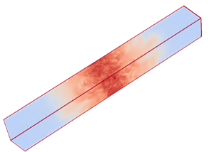
A triply periodic domain of size  $2{\rm \pi} L \times 2{\rm \pi} H \times 2 {\rm \pi}H$ is considered, as shown in figure 1, with $L\gg H$ being along the $x$ direction and $x=0$ taken to be the midplane of the box. The flow inside the domain satisfies the Navier–Stokes equation
 \begin{equation} \partial_t {\boldsymbol{u}} + {\boldsymbol{u}} \boldsymbol{\cdot} \boldsymbol{\nabla} {\boldsymbol{u}} ={-}\boldsymbol{\nabla} P +\nu \nabla^2 {\boldsymbol{u}} + {\boldsymbol{f}}, \end{equation}
where  ${\boldsymbol {u}}$ is the divergence-free velocity field $(\boldsymbol {\nabla }\boldsymbol{\cdot} {\boldsymbol {u}}=0)$, $P$ is the pressure, $\nu$ is the viscosity and ${\boldsymbol {f}}$ is the forcing, with $\boldsymbol {\nabla }\boldsymbol{\cdot} {\boldsymbol {f}}=0$. The functional form of the forcing is given by
 \begin{equation}
{\boldsymbol{f}}(t,{\boldsymbol{x}}) = \left[
\begin{array}{@{}c@{}} 0 \\ \partial_z
[\psi(t,{\boldsymbol{x}}/\ell)-\psi(t,-{\boldsymbol{x}}/\ell)]
\\ \partial_y
[\psi(t,-{\boldsymbol{x}}/\ell)-\psi(t,{\boldsymbol{x}}/\ell)]
\end{array} \right] \exp\left[
\frac{L^2}{\ell^2}\left(\cos\left(\frac{x}{L}\right)
-1\right) \right] ,
\end{equation}
\begin{equation}
{\boldsymbol{f}}(t,{\boldsymbol{x}}) = \left[
\begin{array}{@{}c@{}} 0 \\ \partial_z
[\psi(t,{\boldsymbol{x}}/\ell)-\psi(t,-{\boldsymbol{x}}/\ell)]
\\ \partial_y
[\psi(t,-{\boldsymbol{x}}/\ell)-\psi(t,{\boldsymbol{x}}/\ell)]
\end{array} \right] \exp\left[
\frac{L^2}{\ell^2}\left(\cos\left(\frac{x}{L}\right)
-1\right) \right] ,
\end{equation}
where  $\psi (t,{\boldsymbol {x}}/\ell )$ is a random function including only Fourier modes with wavevectors $\boldsymbol {k}$ satisfying $0<|{\boldsymbol {k}} \ell |\le 2$ and $k_x\ne 0$:
 \begin{equation} \psi(t,{\boldsymbol{x}}/\ell) = \sum_{0<|{\boldsymbol{k}\ell}|\le 2,\, k_x\ne0 } a_{\boldsymbol{k}} \exp({{\rm i}[{\boldsymbol{k}\boldsymbol{\cdot}\boldsymbol{x}} +\phi_{\boldsymbol{k}} (t)]}). \end{equation}
The computational domain considered. The length  $L$ was chosen to be eight times the height, ${L=8H}$, and $x=0$ is taken to be at the middle of the box. The colours indicate visualizations of the enstrophy $(\boldsymbol {\nabla }\times {\boldsymbol {u}})^2$, with red indicating high values while blue represents small values from the $Re_\epsilon =230$ run.

The phases  $\phi _{\boldsymbol {k}}$ of these modes are delta-correlated in time (change randomly every time step $\Delta t$ in the simulation) while the amplitudes $a_{\boldsymbol {k}} \propto 1/\sqrt {\Delta t}$ are fixed in time and independent of $k$. The randomness and the infinitesimal correlation time lead to a mean energy injection rate $\mathcal {I}_0$ independent of the flow. The forcing injects zero momentum at every instant of time. For $|x|\ll L$ the exponential factor to the right of (2.2) scales like $\exp (-x^2/\ell ^2)$ so that the forcing is limited to being only around the range $|x|\sim \ell$ and zero outside. In the numerical simulations that follow, we have picked $\ell =H$ and $L=8H$, which was proven (a posteriori) to be long enough so that the effect of the periodicity along the $x$ direction does not play a role. Periodicity here is used only as a means to reduce computational cost, and in principle other boundary conditions could also be considered.
2.2. Energy balance relations and fluxes in space
The primary quantity of interest in this work is the time- and volume-averaged energy density of the system, which is given by
 \begin{equation} \mathcal{E}_0 = \tfrac{1}{2} \langle \langle |{\boldsymbol{u}}|^2\rangle_{{V}} \rangle_{{T}} , \end{equation}
where the angular brackets  $\langle {\cdot } \rangle _{{T}}$ stand for time average and $\langle {\cdot } \rangle _{{V}}$ for volume average, which are defined as
 \begin{equation} \langle \,f \rangle_{{T}} = \lim_{T\to\infty} \frac{1}{T} \int_0^T f \,{\rm d}t \quad \mathrm{and} \quad \langle \,f \rangle_{{V}} = \frac{1}{V} \int_V f \,{{\rm d}\kern 0.06em x}\,{{\rm d}y}\,{\rm d}z, \end{equation}
with  $V=(2{\rm \pi} )^3H^2L$ being the system volume.
The averaged rate  $\mathcal {I}_0$ at which energy is injected is balanced by the averaged rate $\mathcal {D}_0$ at which energy is dissipated, leading to
 \begin{equation} \mathcal{I}_0 \equiv \langle \langle {\boldsymbol{u}} \boldsymbol{\cdot} {\boldsymbol{f}} \rangle_{{T}} \rangle_{{V}} = 2\nu \langle \langle |{\boldsymbol{S}}|^2 \rangle_{{T}} \rangle_{{V}} \equiv \mathcal{D}_0 , \end{equation}
where  $\boldsymbol {S}$ stands for the strain tensor $S_{i,j} = \frac {1}{2}[ \partial _i u_j + \partial _j u_i ]$.
However, neither the time-averaged energy nor its injection and its dissipation are uniform along the  $x$ direction. It is thus appropriate to consider the mean energy density in a subdomain of the periodic box,
 \begin{equation} \mathcal{E}(X) = \tfrac{1}{2}\langle \langle |{\boldsymbol{u}}|^2 \rangle_{T} \rangle_{X}, \end{equation}
where  $\langle {\cdot } \rangle _{X}$ stands for the average confined in the sub-box from $x=-X$ to $x=X$:
 \begin{equation} \langle \,f \rangle_{X} = \frac{1}{(2{\rm \pi} H)^2} \int_0^{2{\rm \pi} H} \int_0^{2{\rm \pi} H} \int_{{-}X}^X \, f({\boldsymbol{x}},t) \,{{\rm d}\kern 0.06em x}\,{{\rm d}y}\,{\rm d}z. \end{equation}
For  $X={\rm \pi} L$ the entire box is considered, so clearly $\mathcal {E}({\rm \pi} L)=2 {\rm \pi}L \mathcal {E}_0$. We also define the local energy density averaged over the planes $x=\pm X$:
 \begin{equation} E(t,X) = \frac{1}{2(2{\rm \pi} H)^2}\int_0^{2{\rm \pi} H} \int_0^{2{\rm \pi} H} |{\boldsymbol{u}}(t,X,y,z)|^2+|{\boldsymbol{u}}(t,-X,y,z)|^2 \,{\rm d}y\,{\rm d}z . \end{equation}
The two energy densities are related by  $\langle E(X) \rangle _{{T}}=\partial _X \mathcal {E}(X)$.
A generalization of (2.6) for  $\mathcal {E}(X)$ can then be obtained by taking the inner product of the Navier–Stokes equation with ${\boldsymbol {u}}$, time averaging and integrating over $y,z$ and from $x=-X$ to $x=X$ to obtain
 \begin{equation} \mathcal{I}(X) = \mathcal{D}(X) + \mathcal{F}(X), \end{equation}
where  $\mathcal {I}(X)$ and $\mathcal {D}(X)$ are the energy injection rate and the energy dissipation rate within the considered volume defined respectively as
 \begin{equation} \mathcal{I}(X) \equiv \langle \langle \, {\boldsymbol{f}}(t,{\boldsymbol{x}})\boldsymbol{\cdot} {\boldsymbol{u}}(t,{\boldsymbol{x}}) \rangle_X \rangle_T \quad \mathrm{and} \quad \mathcal{D}(X) \equiv 2\nu \langle \langle |{\boldsymbol{S}}(t,{\boldsymbol{x}})|^2 \,{{\rm d}\kern 0.06em x} \rangle_X \rangle_T. \end{equation}
 The third term  $\mathcal {F}(x)$ in (2.10) is a flux that expresses the rate at which energy is transferred outside the considered volume (Landau & Lifshitz Reference Landau and Lifshitz2013). It can be decomposed into three terms
 \begin{equation} \mathcal{F} = \mathcal{F}_U+\mathcal{F}_P+\mathcal{F}_\nu, \end{equation}
where  $\mathcal {F}_U$ is the energy flux due to advection, $\mathcal {F}_P$ is the flux due to pressure and $\mathcal {F}_\nu$ is the flux due to viscosity. They are defined explicitly as
 $$\begin{gather} \mathcal{F}_U(X) = \frac{1}{2(2{\rm \pi} H)^2} \left\langle \int_{x=X} u_x |{\boldsymbol{u}}|^2\, {{\rm d} y}\,{\rm d}z - \int_{x={-}X} u_x |{\boldsymbol{u}}|^2\,{{\rm d}y}\,{\rm d}z \right\rangle_T, \end{gather}$$
 $$\begin{gather}\mathcal{F}_P(X) = \frac{1}{(2{\rm \pi} H)^2} \left\langle \int_{x=X} u_x P\,{{\rm d}y} \,{\rm d}z- \int_{x={-}X}u_x P\, {{\rm d}y} \,{\rm d}z \right\rangle_T, \end{gather}$$
 $$\begin{gather}\mathcal{F}_\nu(X) = \frac{\nu}{(2{\rm \pi} H)^2}\left\langle \int_{{x={-}X}} u_i \partial_i u_x+ u_i \partial_x u_i\,{{\rm d}y}\,{\rm d}z - \int_{{x= X}} u_i \partial_i u_x+ u_i \partial_x u_i\, {{\rm d}y}\,{\rm d}z \right\rangle_T, \end{gather}$$
where the integrals are taken at the two planes  $x=\pm X$ and summation over the index $i$ is assumed in the last one.
2.3. Energy spectra and fluxes in scale space
The fluxes above describe how energy is transported in physical space. At the same time, energy is also transferred in scale space from large to small scales. To quantify the energy distribution and fluxes in scale space, we use the Fourier-transformed fields  $\tilde {\boldsymbol {u}}_{\boldsymbol {k}}(t)$ defined by
 \begin{equation} \tilde{\boldsymbol{u}}_{\boldsymbol{k}}(t) = \langle {\boldsymbol{u}}(t,{\boldsymbol{x}}) \, {\rm e}^{-{\rm i}{\boldsymbol{k}} \boldsymbol{\cdot} {\boldsymbol{x}}} \rangle_{V} \quad\mathrm{and}\quad {\boldsymbol{u}}(t,{\boldsymbol{x}}) = \sum_{{\boldsymbol{k}}} \tilde{\boldsymbol{u}}_{\boldsymbol{k}}(t) \,{\rm e}^{{\rm i} {\boldsymbol{k}} \boldsymbol{\cdot} {\boldsymbol{x}}}, \end{equation}
where the inverse wavenumber  $k^{-1}$ gives a natural definition of a scale. The energy spectrum, giving the distribution of energy among scales is defined as
 \begin{equation} \tilde{E}(k) = \tfrac{1}{2}\sum_{k<|{\boldsymbol{q}}|< k+1} \langle |\tilde{\boldsymbol{u}}_{\boldsymbol{q}}|^2 \rangle_{T}. \end{equation}
The energy flux gives the rate at which energy flows across  $k$ is defined as
 \begin{equation} \varPi(k) ={-}\langle \langle {\boldsymbol{u}}^<_k \boldsymbol{\cdot} {\boldsymbol{u}}\boldsymbol{\cdot}\boldsymbol{\nabla} {\boldsymbol{u}} \rangle_{V}\rangle_{T}, \end{equation}
where  ${\boldsymbol {u}}^<_k$ stands for the velocity field filtered so that only wavenumbers with norm $|{\boldsymbol {k}}|< k$ are retained (Alexakis & Biferale Reference Alexakis and Biferale2018). It is worth noting here the fact that the problem is not homogeneous, making the spectral analysis harder to interpret, and care needs to be taken.
2.4. Reynolds numbers
The Reynolds number in this system provides a measure of the strength of turbulence and it is typically defined as  $Re ={U\ell }/{\nu }$, where $U$ is the typical velocity of the system. In this work, we are interested in the long-box limit, $L \gg H$, and some care needs to be taken in order to be able to compare with homogeneous turbulence results. If we define $U$ based on the mean energy density $\mathcal {E}_0$ (given in (2.4)), then, if turbulence remains localized, $\mathcal {E}_0$ will approach zero in the limit $L\gg H$. Thus defining $U$ as the root mean square (r.m.s.) value over the entire domain, $U=(2\mathcal {E}_0)^{1/2}$, will greatly underestimate the value of $U$ close to the forcing region. The same holds for the mean dissipation rate density $\mathcal {D}_0$.
To compensate for these, we will define the typical velocity  $U$ and the typical dissipation rate $\epsilon$ as
 \begin{equation} U=\sqrt{\frac{2\mathcal{E}_0 L}{H}} \quad\mathrm{and}\quad \epsilon = \mathcal{D}_0 \frac{L}{H}. \end{equation}
The factor  $L/H$ introduced makes $U$ and $\epsilon$ remain finite in the $L/H\to \infty$ limit for localized turbulence. These definitions can be interpreted as the r.m.s. velocity and dissipation around the forcing region.
With these definitions of  $U$ and $\epsilon$, the following three Reynolds numbers typically encountered in the literature are defined:
 \begin{equation} Re_U \equiv \frac{UH}{\nu}, \quad Re_\epsilon \equiv \frac{\epsilon^{1/3} H^{4/3}}{\nu} \quad\mathrm{and}\quad Re_\lambda \equiv \frac{\sqrt{5} U^2}{(\nu\epsilon)^{1/2}}. \end{equation}
The first one is the classical definition of the Reynolds number based on the (rescaled) r.m.s. velocity. The second is a Reynolds number based on the energy injection or dissipation and is the one we control in these simulations (since it is the energy injection rate we impose). Finally, the third one is the Taylor-scale Reynolds number based on the Taylor microscale  $\lambda =U\sqrt {5\nu /\epsilon }$. The three definitions are related by
 \begin{equation} 5Re_U^4 = Re_\lambda^2 Re_\epsilon^{3}, \end{equation}
and for large  $Re_U$ it is expected that $Re_U\propto Re_\epsilon \propto Re_\lambda ^2$.
2.5. Numerical set-up
The Navier–Stokes equations are solved using the pseudospectral code ghost (Mininni et al. Reference Mininni, Rosenberg, Reddy and Pouquet2011), which uses a 2/3 dealiasing rule and a second-order Runge–Kutta method for time advancement. A uniform grid was used such that the grid spacings  $\Delta x = 2{\rm \pi} L/N_x$, $\Delta y = 2{\rm \pi} H/N_y$ and $\Delta z = 2{\rm \pi} H/N_z$ are equal, where $N_x$, $N_y$ and $N_z$ are the numbers of grid points in each direction, with $N_x=8N_y=8N_z$.
The simulations were started from the  ${\boldsymbol {u}}=0$ initial conditions and continued until a steady state is reached, for which a mean energy profile can be calculated. The only exception to this rule is the highest-resolution run $N_x=8192$, for which the results of the $N_x=4096$ run were extrapolated to a larger grid and used as initial conditions. This run was performed for eight turnover times, which was enough to converge sign-definite quantities (like energy) but not sign-indefinite quantities (like fluxes). A run was considered to be well resolved if a viscous exponential decrease in the energy spectrum is observed. We also verified that $k_{max}\eta >1$, where $k_{max}=N_y/3$ in the maximum wavenumber and $\eta =HRe_\epsilon ^{-3/4}$ is the Kolmogorov length scale. The properties of all runs performed are given in table 1.
Resolution and values of the Reynolds numbers  $Re_U$, $Re_\epsilon$ and $Re_\lambda$ achieved in the numerical simulations The last column gives $k_{max}\eta >1$.

3. Results
We begin with figure 2(a), which shows the energy density  $E(t,X)$ for $Re_\epsilon =500$ for different times. The black dashed line shows the forcing profile, which is limited to $|X|/(2{\rm \pi} H)\lesssim 1/2$. Energy spreads away from the forcing region but at late times it fluctuates around a mean profile shown by the red line. Thus already at this stage it can be testified that energy does not spread in the entire box and it remains close to the forcing region. This mean profile is shown in figure 2(b) for different values of $Re_{\epsilon }$. The different colours indicate the different values of the Reynolds number achieved as marked in the key. The same colours are used for all subsequent figures. The peak of the local energy density lies close to the forcing region, $x\simeq 0$, and decays fast away from it. The energy far away from the forcing at $|X|/(2{\rm \pi} H) \simeq 4$ remains very small such that $E(8{\rm \pi} H)/E(0)\lesssim 10^{-6}.$
(a) The energy density  $E(t,X)$ for different times for $Re_\epsilon =500$. Times are in units of $H^{2/3}/\epsilon ^{1/3}$. (b) The time-averaged energy density $\langle E(X) \rangle _{T}$ at steady state for different values of $Re_\epsilon$ in the entire domain. The dashed line indicates the forcing amplitude as a function of $X$. The inset shows the same data in log–log scale. The same colour key is used to mark $Re_\epsilon$ in all subsequent figures.

Before continuing with spatial properties of our flow, we perform some standard benchmark analysis often used in homogeneous turbulence. Figure 3 shows the scaling of global measures as a function of the Reynolds number. Figure 3(a) shows the relation between the different Reynolds numbers where the scaling  $Re_U\propto Re_\epsilon \propto Re_\lambda ^2$ that holds for large $Re$ is verified. In figure 3(b) we show the non-dimensional dissipation rate (or drag coefficient) $C_\epsilon$ defined here as
 \begin{equation} C_\epsilon = \frac{\epsilon H}{U^3}, \end{equation}
which expresses the rate at which energy is dissipated non-dimensionalized by the amplitude of the fluctuations.
(a) Relation between the different Reynolds numbers  $Re_U$, $Re_\epsilon$ and $Re_\lambda$. (b) The normalized dissipation rate $C_f$ as a function of $Re_\lambda$.

It is a cornerstone conjecture of homogeneous and isotropic turbulence theory that  $C_\epsilon$ attains a finite and $Re$-independent value at large $Re$. The present data indicate that, at large $Re_\lambda$, $C_\epsilon$ appears to converge to a $Re_\lambda$-independent value but quite slowly. Only the largest values of $Re_\lambda \gtrsim 270$ indicate the possibility that such a plateau is reached, with a value of $C_\epsilon \simeq 0.06$ that is rather small. In homogeneous and isotropic simulations, such a plateau is reached after $Re_\lambda \sim 100$ and at a much larger value $C_\epsilon \simeq 0.5$ (Kaneda et al. Reference Kaneda, Ishihara, Yokokawa, Itakura and Uno2003). This reflects that localized turbulence is affected by the additional freedom to expand in a larger region, possibly suppressing its efficiency to cascade energy to the smaller scales.
Figure 4 examines spectral properties of the flow. In figure 4(a) we plot the energy spectra for the different values of  $Re$. Despite the strong inhomogeneity, the spectra show similar behaviour to homogeneous turbulence flows. As the Reynolds number is increased, more scales are excited and a power-law spectrum starts to form, with exponent close to the Kolmogorov prediction ${\tilde {E}}(k)\propto k^{-5/3}$. In figure 4(b) the energy fluxes in Fourier space are plotted. The energy fluxes increase with $Re$ until, for the largest $Re$s attained, a constant-flux range has begun to form. It is worth noting that this constant-flux region is obtained at much larger $Re$ than is observed in homogeneous turbulence, reflecting a delay in obtaining a $Re$-independent scaling due to the effect of spreading.
(a) The energy spectra  $\tilde {E}(k)$ for the different $Re_\lambda$ examined. (b) The energy fluxes $\varPi (k)$ for the same runs.

Returning to the spatial properties of the flow and the energy density profile, we note that, as the Reynolds number is increased, the energy increases and also spreads at larger distances. At very large values of  $Re_\lambda$, the energy profile appears to converge to a $Re$-independent profile. This implies that at large $Re$ the energy profile is determined by the self-spreading of eddies due to turbulent advection and not by viscous processes. The fast drop of $E(X)$ can be either an exponential, $E(x)\propto \exp (-\alpha x)$, or a steep power law, $E(x)\propto |X|^{-6}$ (see inset). The present data cannot exclude either option. We point out that, since the energy density drops very fast, the local Reynolds number (defined using a local r.m.s. velocity) is also decreasing. So it is hard to obtain a large- $Re$ behaviour in the outer region $|X| \gg H$.
The fact that the energy density reaches a  $Re$-independent profile is not a trivial result. It reflects a balance between the rate at which energy is transported to larger values of $|x|$ and the rate at which energy cascades to the small scales. If the cascade process was weaker than the real-space transport, then in the $Re\to \infty$ limit energy would reach the entire domain. On the contrary, if the real-space transport was weaker, no energy would be found outside the forcing region in the same limit. In other words, turbulent diffusion and turbulent dissipation must be of the same order.
To quantify this assertion, we look at the fluxes in real space. In figure 5 we plot  $\mathcal {F}_i$ for three different values of $Re$, varying from the laminar to the turbulence case. In each panel, the black line shows the total flux, the blue line the flux due to velocity fluctuations, the green line the flux due to pressure and the red line the flux due to viscosity. The magenta line shows the difference between $\mathcal {I}(X)$ and $\mathcal {D}(X)$. A comparison between the black and magenta lines verifies the relation (2.10). The small differences that are observed are due to insufficient time averaging, which is more pronounced in the large resolution runs.
The different energy fluxes in real space as indicated in the legend for three different values of  $Re_\epsilon =4$ (a), 40 (b) and 500 (c).

A few observations need to follow. For small  $Re$, the energy flux is dominated by viscosity, with pressure also playing a significant part. The flux due to the velocity fluctuations has a negative sign. As the Reynolds number is increased, the role of the velocity fluctuations becomes more dominant, transferring energy outwards. The transfer due to viscosity diminishes while the transfer due to pressure also takes negative values. At the largest $Re$, almost the entire flux is dominated by the velocity fluctuations, with the pressure flux being weaker and positive in the forcing region and negative away from it. The behaviour and functional form of these fluxes remain puzzling, in particular the negative pressure flux, which implies that high pressure fluctuations are correlated with inner-directed velocities. A theoretical understanding of these fluxes needs to be pursued by future theoretical work.
Finally, to compare the two dominant processes away from the forcing region, i.e. turbulent dissipation and turbulent diffusion, we plot the dissipation rate  $\mathcal {D}(X)$ in figure 6(a) and the total flux $\mathcal {F}(X)$ in figure 6(b) for all $Re$. Figure 6(c) compares the two, for $Re_\epsilon =500$. The black dashed lines indicate $\mathcal {I}(X)$, which is the same for all $Re$. As the Reynolds number is increased, the dissipation is decreased while the flux is increased. For the largest $Re$ at the peak of the flux around $X\simeq 0.15 (2{\rm \pi} H)$, the two processes become approximately equal, marking that the two processes, turbulent dissipation and turbulent diffusion, are of the same order.
(a) The dissipation rate  $\mathcal {D}(X)$, and (b) the energy flux $\mathcal {F}(X)$ for different values of $Re$. (c) Comparison of the largest $Re_\epsilon =500$ for which the fluxes were measured. The black dashed lines indicate $\mathcal {I}(X)$.

4. Conclusions
The present work has demonstrated that locally forced turbulence will not spread throughout the domain provided that there is no mean injection of linear or angular momentum. It will remain localized, forming an energy density profile that is  $Re$-independent in the large- $Re$ limit. Away from the forcing region, the two dominant effects are turbulent dissipation and turbulent diffusion, which were found to be of the same order. Whether the resulting profile is universal or depends on the details of the forcing mechanisms remains to be seen.
To expand upon the understanding of the two processes involved, turbulent diffusion and turbulent dissipation, a simultaneous scale-space and real-space analysis would be required, either by introducing local smoothing (Germano Reference Germano1992; Aluie & Eyink Reference Aluie and Eyink2009; Eyink & Aluie Reference Eyink and Aluie2009; Alexakis & Chibbaro Reference Alexakis and Chibbaro2020) or by using two-point analysis and the Kármán–Howarth–Monin–Hill equation (Hill Reference Hill2001, Reference Hill2002). The latter has been used recently to study boundary-driven flows (Apostolidis et al. Reference Apostolidis, Laval and Vassilicos2022, Reference Apostolidis, Laval and Vassilicos2023) and wakes (Chen et al. Reference Chen, Cuvier, Foucaut, Ostovan and Vassilicos2021; Chen & Vassilicos Reference Chen and Vassilicos2022), where the role of inhomogeneous energy injection from the mean flow was emphasized. In the present flow, there is no mean flow and the primary terms in balance are the inter-scale transfer rate and turbulent transport in physical space, both of which are forcing- and viscosity-independent. Thus a new state of turbulence is present, where two inertial effects, the energy fluxes in scale space and in real space, compete.
Simplified models such as Reynolds-averaged Navier–Stokes and the  $K$–
$K$– $\epsilon$ model (Lele Reference Lele1985; Speziale Reference Speziale1998; Yusuf et al. Reference Yusuf, Asako, Sidik, Mohamed and Japar2020) could also help in predicting the resulting energy profile. Such models depend on parametrizing the energy cascade and the energy diffusion, the two effects whose balance leads to the energy profile. Care thus needs to be taken in this parametrization so that the correct energy profile is captured.
Finally, we would like to add that the present study was limited to a flow in an anisotropic box elongated along one direction. This restricts the spreading of turbulence only along this direction. Its extension to larger domains where turbulence can spread in two or in all three directions is far from trivial and would need to be examined separately. Here experimental investigations would become much more beneficial than numerical simulations.
Funding
This work was granted access to the HPC resources of GENCI-TGCC and GENCI-CINES (Project No. A0130506421). This work has also been supported by the Agence nationale de la recherche (ANR projects DYSTURB No. ANR-17-CE30-0004 and LASCATURB No. ANR-23-CE30).
Declaration of interest
The author reports no conflict of interest.


 Open access