





1. Introduction
Geophysical flows are characterized by rapid rotation of the frame of reference and by density stratification in the vertical direction. In the mid-latitudes, the dominant force balance is between the Coriolis force due to rotation and the pressure gradient forces. The leading-order concept, geostrophic balance, is exact in linearized dynamics; corrections beyond the leading order are more subtle, as nonlinear interactions begin to play a role. In practical terms, a well-balanced state is one that minimizes fast geostrophic adjustment by gravity wave activity in its subsequent time evolution.
The necessity to provide balanced initial conditions was recognized early in the development of numerical weather prediction (see, e.g. Lynch Reference Lynch2006 for a historical account). Machenhauer (Reference Machenhauer1977) and Baer & Tribbia (Reference Baer and Tribbia1977) pioneered the idea of nonlinear normal mode initialization, where Machenhauer obtained the first consistent nonlinear correction to a linear mode decomposition, which corresponds to the quasi-geostrophic balanced state (Leith Reference Leith1980). Baer and Tribbia, in the same year, proposed a multiple time-scale expansion which produces consistent higher-order balance relations and gave explicit second-order expressions. Warn et al. (Reference Warn, Bokhove, Shepherd and Vallis1995) revisit the problem from a more abstract perspective, see § 3.1 below. They reformulate the procedure without the need to introduce explicit fast-time and slow-time variables, and raise the issue that the resulting series is asymptotic, but not necessarily convergent.
Geometrically, a balance relation defines a slow manifold. A slow manifold is a submanifold of the phase space on which the solution trajectory evolves more slowly than anywhere else. For systems with a small asymptotic order parameter, ‘more slowly’ is usually defined as ‘increases at a lower asymptotic rate as the order parameter goes to zero’. In the well-studied case of so-called normally hyperbolic systems – the van der Pol oscillator being a classical example – slow manifolds are attracting, unique and exactly invariant. In this situation, it is possible to reduce the dynamics exactly to a dynamical system of lesser dimension on the slow manifold. Large-scale geophysical fluid flow, on the other hand, is essentially inviscid. The Kolmogorov scale at which molecular viscosity becomes relevant is so far removed from the scales of interest that, for the purpose of characterizing balance, we need to work in the conceptual framework of Hamiltonian dynamics.
For Hamiltonian systems, the existence of exactly invariant slow manifolds is too much to hope for. MacKay (Reference MacKay2004), for example, constructs an elementary example which shows that an exactly invariant slow manifold cannot survive small generic Hamiltonian perturbations. He argues that a useful notion of slow manifold should include any submanifold of phase space with the following properties:
(i) The vector field is approximately tangent to the manifold, i.e. the manifold is nearly invariant.
(ii) The component of the vector field normal to the manifold grows strongly away from the manifold, i.e. the typical dynamic time scale off the manifold is much faster than the time rate of change on the manifold.
In this framework, slow manifolds are not unique. One slow manifold may be better than another in the sense that the approximate invariance of the manifold under the flow is more accurate. Often, a hierarchy of slow manifolds is given by an asymptotic series. In this situation, non-existence of an exactly invariant slow manifold is seen through the divergence of the asymptotic series. Yet, applying optimal truncation, exponential smallness of remainders can often be proved – see, e.g. Vanneste & Yavneh (Reference Vanneste and Yavneh2004) for exponential asymptotics of a simple model equation, Vanneste (Reference Vanneste2013) for a review from the geophysical fluid dynamics perspective and MacKay (Reference MacKay2004) and references therein for a more mathematical perspective.
For a practical decomposition of the state variables into their balanced and unbalanced components, an optimal truncation of the divergent series is not directly available. Therefore, high-accuracy diagnostics will either need to use a fixed, but possibly higher-order balance, or rely on a purely numerical proxy for optimal truncation, known as optimal balance. Regarding the first practical method, fixed higher-order asymptotics, Chouksey, Eden & Brüggemann (Reference Chouksey, Eden and Brüggemann2018) have shown that, in order to diagnose the true gravity wave signal of waves emitted from an unstable jet, the residual of the first-order balance obtained from the nonlinear normal mode initialization procedure of Machenhauer (Reference Machenhauer1977) is still dominated by slaved (slow) modes, not by the true wave signal, which only becomes visible at third or fourth order (Eden, Chouksey & Olbers Reference Eden, Chouksey and Olbers2019a), if at all. This is of relevance since wave emission is proposed as a significant sink of meso-scale eddy energy globally in the ocean from laboratory experiments (Williams, Haine & Read Reference Williams, Haine and Read2008) and idealized numerical simulations (Brüggemann & Eden Reference Brüggemann and Eden2015; Sugimoto & Plougonven Reference Sugimoto and Plougonven2016), but it is possible that the signals discussed in those experiments are related to the so-called slaved modes and not to actual wave emission.
The second practical method for computing balance was pioneered by Viúdez & Dritschel (Reference Viúdez and Dritschel2004). Their optimal potential vorticity balance (OPV balance) was first conceived as a modification of a Lagrangian contour-advecting numerical code in which the perturbation potential vorticity is slowly ‘ramped’ from a trivial state to a fully nonlinear state ‘in which the amount of inertia–gravity waves is minimal’, but the original approach by Viúdez and Dritschel can be formulated for any model code as shown below. The approach is attractive because it produces high quality balance without any explicit asymptotics at non-trivial, but moderate computational expense, and is relatively easy to implement for a given numerical code.
Cotter (Reference Cotter2013) realized that Viúdez and Dritschel's procedure can be understood theoretically in terms of adiabatic invariance in the following sense: a trajectory that is initially close to a slow manifold, thus evolving approximately along this manifold, will continue to do so when the manifold is deformed slowly in time. Cotter provided proof, in the context of a finite-dimensional Hamiltonian system, that the resulting balance is exponentially accurate, just as balance itself can only be defined up to exponentially small remainders. His argument presumes that the required integration is performed over an unbounded interval of time. Gottwald, Mohamad & Oliver (Reference Gottwald, Mohamad and Oliver2017) studied optimal balance for the same finite-dimensional model restricted to a finite interval of time, which is necessary for any practical implementation. They realized that the required ramp function must satisfy consistency conditions at the temporal end points that preclude the use of analytic normal form theory for the mathematical analysis. Yet, they were able to prove exponential estimates, albeit with a smaller power of the time separation parameter in the exponent. Thus, the state produced by ‘optimal balance’ (here not ‘OPV balance’ because the principle goes beyond a potential vorticity formulation of the problem) is not optimal in the strict sense, but very good in the sense that the remainder is small beyond all orders, and arguably the best practically accessible algorithm for flow separation.
In this study, we compare the higher-order balancing method by Warn et al. (Reference Warn, Bokhove, Shepherd and Vallis1995) with the optimal balance method by Masur & Oliver (Reference Masur and Oliver2020) using two different discretizations of the single-layer shallow water equations, and for two qualitatively different initial states. In the following section, the model equations and their spectral representation are specified. Both methods are re-derived within the same framework in § 3. It turns out that they can both be understood as a correction to the linear geostrophic mode  $\boldsymbol {z}_0$ for the nonlinear model, using only $\boldsymbol {z}_0$ itself. In § 4, the numerical codes, our model diagnosis strategy and the initial conditions are detailed. Section 5 presents the results of the comparison. The paper concludes with a short discussion.
2. Model description
2.1. The single-layer model
As a simple test case, we take a reduced gravity model for a single layer of constant density with mean height  $H_0$. The dimensional equations of motion for velocity $\boldsymbol {u}$ and perturbation height $h$ are given by
 $$\begin{gather} \partial_t \boldsymbol{u} + \boldsymbol{u} \boldsymbol{\cdot} \boldsymbol{\nabla} \boldsymbol{u} + f \, \boldsymbol{u}^\bot + g \, \boldsymbol{\nabla} h = 0 , \end{gather}$$
 $$\begin{gather}\partial_t h + H_0 \boldsymbol{\nabla} \boldsymbol{\cdot} \boldsymbol{u} + \boldsymbol{\nabla} \boldsymbol{\cdot} (h\boldsymbol{u}) = 0 , \end{gather}$$
where  $\boldsymbol {u}^\bot$ denotes anticlockwise rotation of the vector $\boldsymbol {u}=(u,v)$ by ${\rm \pi} /2$, i.e. $\boldsymbol {u}^\bot =(-v, u)$, $f$ is the Coriolis parameter and $g$ the acceleration due to gravity. We non-dimensionalize (2.1) in terms of the usual Rossby ( ${\textit {Ro}}$), Burger ( ${\textit {Bu}}$) and Froude ( ${\textit {Fr}}$) numbers
 \begin{equation} {\textit{Ro}} = \frac{U}{f_0 L} , \quad {\textit{Bu}} = \frac{{\textit{Ro}}^2}{{\textit{Fr}}^2} , \quad \text{and} \quad {\textit{Fr}} = \frac{U}c, \end{equation}
where  $f_0$ denotes the constant background rate of rotation and $c^2 = gH_0$ is the phase speed of gravity waves in the high wavenumber limit. Also, $U$ and $L$ denote the horizontal velocity scale and length scale, respectively. Assuming that Coriolis and pressure gradient forces approximately balance and choosing the fast time scale associated with the propagation of gravity waves, we have
 $$\begin{gather} \partial_t \boldsymbol{u} + f \, \boldsymbol{u}^\bot + \boldsymbol{\nabla} h ={-} {\textit{Ro}}\, \boldsymbol{u} \boldsymbol{\cdot} \boldsymbol{\nabla} \boldsymbol{u} , \end{gather}$$
 $$\begin{gather}\partial_t h + {\textit{Bu}}\, \boldsymbol{\nabla} \boldsymbol{\cdot} \boldsymbol{u} ={-} {\textit{Ro}}\, \boldsymbol{\nabla} \boldsymbol{\cdot} (h\boldsymbol{u}) , \end{gather}$$
where all symbols refer to non-dimensional quantities. We now assume a constant rate of rotation, taking the scaled Coriolis parameter  $f=1$ and choose the quasi-geostrophic distinguished limit by setting ${\textit {Bu}}=1$.
2.2. Normal mode representation
We consider the model on a doubly periodic square domain of length  $2 {\rm \pi}$. Using the Fourier representation
 \begin{equation} \boldsymbol{u} (\boldsymbol{x}, t) = \sum_{{\boldsymbol{k}} \in \mathbb{Z}^2} \boldsymbol{u}_{\boldsymbol{k}} (t) \exp({\mathrm{i} {\boldsymbol{k}} \boldsymbol{\cdot} \boldsymbol{x}}), \end{equation}
where the complex coefficients satisfy  $\boldsymbol {u}_{-{\boldsymbol {k}}} = \boldsymbol {u}^*_{\boldsymbol {k}}$ so that $\boldsymbol {u}(\boldsymbol {x},t)$ is real, with a corresponding representation for $h$, writing $\boldsymbol {z}_{\boldsymbol {k}} = (u_{\boldsymbol {k}}, v_{\boldsymbol {k}}, h_{\boldsymbol {k}})$, and denoting the vector of all Fourier coefficients by $\boldsymbol {z} = (\boldsymbol {z}_{\boldsymbol {k}})_{{\boldsymbol {k}} \in \mathbb {Z}^2}$, we write (2.3) in the form
 \begin{equation} \frac{\mathrm{d}\boldsymbol{z}}{\mathrm{d} t} = \mathrm{i} \boldsymbol{A} \boldsymbol{z} + {\textit{Ro}} \boldsymbol{N}(\boldsymbol{z}, \boldsymbol{z}) . \end{equation}
The system matrix  $\boldsymbol{A}$ is given by
 \begin{equation} \boldsymbol{A}_{\boldsymbol{k}} = \begin{pmatrix} 0 & -\mathrm{i} & - k \\ \mathrm{i} & 0 & - \ell \\ -{\textit{Bu}} \, k & - {\textit{Bu}} \ell & 0 \end{pmatrix} , \quad \boldsymbol{A} = (\boldsymbol{A}_{\boldsymbol{k}} )_{{\boldsymbol{k}} \in \mathbb{Z}^2} , \quad {\boldsymbol{k}}=(k, \ell) \end{equation}
and the nonlinear interactions  $\boldsymbol {N}(\boldsymbol {z}, \boldsymbol {z}) = (\boldsymbol {N}_{\boldsymbol {k}})_{{\boldsymbol {k}} \in \mathbb {Z}^2}$ are given by the symmetric bilinear form
 \begin{equation} \boldsymbol{N}_{\boldsymbol{k}} (\boldsymbol{z}, \boldsymbol{z}') ={-} \frac{\mathrm{i}}2 \sum_{{\boldsymbol{\ell}} + {\boldsymbol{m}} = {\boldsymbol{k}}} \begin{pmatrix} \boldsymbol{u}_{\boldsymbol{m}} {\boldsymbol{m}} \boldsymbol{\cdot} \boldsymbol{u}_{\boldsymbol{\ell}}' + \boldsymbol{u}_{\boldsymbol{m}}' {\boldsymbol{m}} \boldsymbol{\cdot} \boldsymbol{u}_{\boldsymbol{\ell}} \\ h_{\boldsymbol{m}} {\boldsymbol{k}} \boldsymbol{\cdot} \boldsymbol{u}_{\boldsymbol{\ell}}' + h_{\boldsymbol{m}}' {\boldsymbol{k}} \boldsymbol{\cdot} \boldsymbol{u}_{\boldsymbol{\ell}}, \end{pmatrix} \end{equation}
where  $\boldsymbol {z}'$ is a second coefficient vector with components $\boldsymbol {u}_{\boldsymbol {k}}'$ and $h_{\boldsymbol {k}}'$ and $\boldsymbol{A}$ denotes the infinite block-diagonal matrix made of components $\boldsymbol{A}_{\boldsymbol {k}}$ with corresponding ordering to fit to $\boldsymbol {z} = (\boldsymbol {z}_{\boldsymbol {k}})_{{\boldsymbol {k}} \in \mathbb {Z}^2}$. The expression for $\boldsymbol {N}_{\boldsymbol {k}}$ has been symmetrized, which is not necessary at this point, but makes it easy to separate the interactions between different modes as in (2.12) below.
The matrix  $\boldsymbol{A}_{\boldsymbol {k}}$ has three eigenvalues $\omega ^0_{\boldsymbol {k}} = 0$ and $\omega ^\pm _{\boldsymbol {k}} = \pm \sqrt {1 + {\textit {Bu}} \lvert {\boldsymbol {k}} \rvert ^2}$. Two of them, $\omega ^{\pm }$, correspond to inertia–gravity waves, henceforth referred to as gravity waves for short. The other one, $\omega ^{0}$, corresponds to a vortical mode, sometimes also referred to as the Rossby mode or Rossby wave (here, it is a zero-frequency ‘wave’ since the $f$ is constant.) In the more general case when $f$ is slowly varying in space, the Rossby wave frequency is finite but remains much smaller than $\lvert \omega ^{\pm } \rvert$ (see, e.g. appendix B of Eden, Chouksey & Olbers (Reference Eden, Chouksey and Olbers2019b) for an expression using first-order perturbation theory).
The corresponding left and right eigenvectors, satisfying  $(\boldsymbol {p}^{\sigma }_{\boldsymbol {k}})^\boldsymbol{H} \boldsymbol{A}_{\boldsymbol {k}} = (\boldsymbol {p}^{\sigma }_{\boldsymbol {k}})^\boldsymbol{H} \omega ^\sigma _{\boldsymbol {k}}$ and $\boldsymbol{A}_{\boldsymbol {k}} \boldsymbol {q}^\sigma _{\boldsymbol {k}} = \omega ^\sigma _{\boldsymbol {k}} \boldsymbol {q}^\sigma _{\boldsymbol {k}}$ for $\sigma = 0, -, +$ are (see, e.g. Eden et al. Reference Eden, Chouksey and Olbers2019b)
 \begin{equation} \boldsymbol{q}^{\sigma}_{\boldsymbol{k}} = \begin{pmatrix} \dfrac{\sigma \lvert \omega \rvert {\boldsymbol{k}} + \mathrm{i} {\boldsymbol{k}}^\bot} {1 - \sigma^2 \, \omega^2} \\ 1 \vphantom{\dfrac11} \end{pmatrix} , \quad \boldsymbol{p}^\sigma_{\boldsymbol{k}} = n^\sigma_{\boldsymbol{k}} \begin{pmatrix} \dfrac{\sigma \lvert \omega \rvert {\boldsymbol{k}} + \mathrm{i} {\boldsymbol{k}}^\bot} {1 - \sigma^2 \omega^2} \\ {\textit{Bu}}^{{-}1} \vphantom{\dfrac11}, \end{pmatrix} \end{equation}
with normalization
 \begin{equation} n^\sigma_{\boldsymbol{k}} = \frac{{\textit{Bu}}}{1+\sigma^2} \frac{\lvert \sigma^2 \omega^2-1 \rvert} {1 + {\textit{Bu}} \lvert {\boldsymbol{k}} \rvert^2}, \end{equation}
so that orthonormality holds, i.e.  $(\boldsymbol {p}^\sigma _{\boldsymbol {k}})^\boldsymbol{H} \, \boldsymbol {q}^{\sigma '}_{\boldsymbol {k}} = \delta _{\sigma,\sigma '}$. The superscript $\boldsymbol{H}$ denotes the Hermitian conjugate. We write $\mathbb {P}^0$ to denote the orthogonal projector onto the vortical modes, and $\mathbb {P}^+$ and $\mathbb {P}^-$ to denote the orthogonal projector onto each of the gravity wave modes, given for every fixed wavenumber ${\boldsymbol {k}}$ by
 \begin{equation} \mathbb{P}^\sigma_{\boldsymbol{k}} = \boldsymbol{q}_{\boldsymbol{k}}^\sigma (\boldsymbol{p}_{\boldsymbol{k}}^\sigma)^\boldsymbol{H}, \quad \text{for } \sigma = 0, -, + , \end{equation}
set  $\boldsymbol {z}^\sigma = \mathbb {P}^\sigma \boldsymbol {z}$, $\boldsymbol {N}^\sigma = \mathbb {P}^\sigma \boldsymbol {N}$ and introduce the short-hand notation $\mathbb {P}^{gw} = \mathbb {P}^+ + \mathbb {P}^-$ and $\boldsymbol {z}^{gw} = \boldsymbol {z}^+ + \boldsymbol {z}^-$. In the basis of right eigenvectors, the linear part of the components of (2.5) is diagonal, so that
 \begin{equation} \frac{\mathrm{d} \boldsymbol{z}^\sigma_{\boldsymbol{k}}}{\mathrm{d} t} - \mathrm{i} \omega^{\sigma}_{\boldsymbol{k}} \boldsymbol{z}^\sigma_{\boldsymbol{k}} = {\textit{Ro}} \boldsymbol{N}^\sigma_{\boldsymbol{k}} (\boldsymbol{z}, \boldsymbol{z}) , \end{equation}
where the case  $\sigma =0$ corresponds to the slow (vortical) modes and $\sigma =\pm$ to the fast (gravity wave) modes. We note that
 $$\begin{gather} \boldsymbol{N}^\sigma(\boldsymbol{z}, \boldsymbol{z}) = \boldsymbol{N}^\sigma(\boldsymbol{z}^0, \boldsymbol{z}^0) + 2 \boldsymbol{N}^\sigma(\boldsymbol{z}^0, \boldsymbol{z}^{gw}) + \boldsymbol{N}^\sigma(\boldsymbol{z}^{gw}, \boldsymbol{z}^{gw}) , \end{gather}$$
so that we can sort the nonlinear interactions into vortical–vortical, vortical–gravity and gravity–gravity mode interactions. Due to this coupling, an accurate description of the slow manifold will involve not only the linear geostrophic modes  $\boldsymbol {z}^0$, but also some non-zero contributions in the linear gravity wave modes $\boldsymbol {z}^{gw} = \boldsymbol {z}^+ + \boldsymbol {z}^-$.
3. Nonlinear high-order balance
3.1. Higher-order balance procedure
We assume a state in which the gravity waves are initially small, namely  $\boldsymbol {z}^{\pm } = O({\textit {Ro}})$. Accordingly, we expand the gravity wave amplitudes as
 \begin{equation} \boldsymbol{z}^{{\pm}} = {\textit{Ro}} \boldsymbol{z}_1^{{\pm}} + {\textit{Ro}}^2 \boldsymbol{z}_2^{{\pm}} + {\textit{Ro}}^3 \, \boldsymbol{z}_3^{{\pm}}+ \cdots . \end{equation}
It can be shown that, under this assumption, the gravity wave amplitudes are growing only weakly in time, so that this ansatz remains consistent for an extended period of (slow) time.
The time derivative in (2.5) includes fast gravity waves with frequency  $\omega ^{\pm }$ and the slow growth and decay of the amplitudes of both slow and fast modes due to the nonlinear interactions. Therefore, we introduce a slow time variable $s = {\textit {Ro}} \, t$ so that $\mathrm {d}/\mathrm {d} t = \partial _t + {\textit {Ro}} \partial _s$.
Assume now that  $\boldsymbol {z}^0$ is a function of slow time only, whereas $\boldsymbol {z}^{\pm }$ is a function of slow and fast times. Thus, (2.11) for the vortical mode $\sigma =0$ reads
 \begin{equation} {\textit{Ro}} \partial_s \boldsymbol{z}^{0} = {\textit{Ro}} \boldsymbol{N}^0(\boldsymbol{z}, \boldsymbol{z}) . \end{equation}
Using (2.12) and inserting the expansion (3.1), we see that the leading order of (3.2) is given by
 \begin{equation} \partial_s \boldsymbol{z}^{0} = \boldsymbol{N}^{0} (\boldsymbol{z}^0, \boldsymbol{z}^0) . \end{equation}
This first-order balanced model is identical to the familiar (first-order) quasi-geostrophic approximation, as observed by Leith (Reference Leith1980). Only the vortical modes  $\boldsymbol {z}^0$ are involved, and this is why (3.3) – which is a spectral representation of the quasi-geostrophic potential vorticity equation – is closed.
To obtain a model which is second- or higher-order accurate, diagnostic relations for the ageostrophic balanced modes or slaved modes  $\boldsymbol {z}^{\pm }_n$ need to be derived. These modes are part of the balanced motion since they evolve only slowly (Warn et al. Reference Warn, Bokhove, Shepherd and Vallis1995; McIntyre & Norton Reference McIntyre and Norton2000; Kafiabad & Bartello Reference Kafiabad and Bartello2018). The lowest order of these, $\boldsymbol {z}^{\pm }_1$, corresponds to the first-order (ageostrophic) variables in the quasi-geostrophic approximation (Leith Reference Leith1980), which are not needed to predict the evolution of the geostrophic variables and generally unknown in the quasi-geostrophic model. However, they are required for all higher-order balance models.
To first order in  ${\textit {Ro}}$, (2.5) for the gravity wave modes reads
 \begin{equation} \partial_{t} \boldsymbol{z}_1^{{\pm}} - \mathrm{i} \, \omega^{{\pm}} \, \boldsymbol{z}_1^{{\pm}} = \boldsymbol{N}^{{\pm}} (\boldsymbol{z}^0, \boldsymbol{z}^0) , \end{equation}
where  $\omega ^\pm$ denotes the diagonal operator acting as multiplication by $\omega ^+_{\boldsymbol {k}}$ or $\omega ^-_{\boldsymbol {k}}$, respectively, on each of the eigenspaces.
A non-zero time derivative in (3.4) reflects the existence of fast waves with frequency  $\omega ^\pm$. Thus, to enforce a balanced state, it is necessary to have
 \begin{equation} \boldsymbol{z}_1^{{\pm}} = \mathrm{i} \boldsymbol{N}^{{\pm}} (\boldsymbol{z}^0, \boldsymbol{z}^0) / \omega^{{\pm}} . \end{equation}
Inserting this relation back into (2.5), we obtain a second-order balance model of the form
 \begin{equation} \partial_s \boldsymbol{z}^{0} = \boldsymbol{N}^{0} (\boldsymbol{z}^0, \boldsymbol{z}^0) + 2 {\textit{Ro}} \boldsymbol{N}^0(\boldsymbol{z}^0, \boldsymbol{z}^{gw}_1) . \end{equation}
Setting  $\partial _{t} \boldsymbol {z}^{\pm }_n=0$ to suppress generation of gravity waves in general, we write (2.11) as
 $$\begin{gather} \sum_{n=1}^\infty ({\textit{Ro}}^{n+1} \partial_s - \mathrm{i} \omega^{{\pm}} {\textit{Ro}}^n) \boldsymbol{z}_n^{{\pm}} = {\textit{Ro}} \boldsymbol{N}^\pm (\boldsymbol{z}^0, \boldsymbol{z}^0) \nonumber\\ + 2 \sum_{n=1}^\infty {\textit{Ro}}^{n+1} \boldsymbol{N}^\pm (\boldsymbol{z}^0, \boldsymbol{z}_n^{gw}) + \sum_{n=2}^\infty {\textit{Ro}}^{n+1} \sum_{i+j=n} \boldsymbol{N}^\pm (\boldsymbol{z}_i^{gw}, \boldsymbol{z}_j^{gw}), \end{gather}$$
with  $\boldsymbol {z}^{gw}_n= \boldsymbol {z}^+_n + \boldsymbol {z}^-_n$. In particular, the second, third and fourth orders are given by
 $$\begin{gather} \partial_s \boldsymbol{z}_1^{{\pm}} - \mathrm{i} \omega^{{\pm}} \, \boldsymbol{z}_2^{{\pm}} = 2 \boldsymbol{N}^{{\pm}}(\boldsymbol{z}^0, \boldsymbol{z}_1^{gw}) \end{gather}$$
 $$\begin{gather}\partial_s \boldsymbol{z}^{{\pm}}_2 - \mathrm{i} \omega^{{\pm}} \, \boldsymbol{z}_3^{{\pm}} = 2 \boldsymbol{N}^\pm(\boldsymbol{z}^0, \boldsymbol{z}_2^{gw}) + \boldsymbol{N}^{{\pm}}(\boldsymbol{z}_1^{gw}, \boldsymbol{z}_1^{gw}) \end{gather}$$
 $$\begin{gather}\partial_s \boldsymbol{z}^{{\pm}}_3 - \mathrm{i} \omega^{{\pm}} \boldsymbol{z}_4^{{\pm}} = 2 \boldsymbol{N}^\pm(\boldsymbol{z}^0, \boldsymbol{z}_3^{gw}) + 2 \boldsymbol{N}^{{\pm}}(\boldsymbol{z}_1^{gw}, \boldsymbol{z}_2^{gw}) . \end{gather}$$
Hence, we can calculate  $\boldsymbol {z}_2^{\pm }$ from (3.8a), $\boldsymbol {z}_3^{\pm }$ from (3.8b) and so on. The slow time derivative $\partial _s \boldsymbol {z}_1^{\pm }$ in (3.8a) is calculated analytically by taking the derivative of (3.5) and inserting (3.3) as outlined in Kafiabad & Bartello (Reference Kafiabad and Bartello2018) and Eden et al. (Reference Eden, Chouksey and Olbers2019a, § 2); $\partial _s \boldsymbol {z}_2^{\pm }$ and higher are calculated by integrating the model with (the inverse Fourier transform of) $\boldsymbol {z}_0 + {\textit {Ro}} \boldsymbol {z}^{gw}_1$ as initial condition for a few time steps and taking a finite difference. Since only slow time derivatives $\partial _s$ show up, the slaved modes (or ageostrophic balanced modes) $\boldsymbol {z}_n^{gw} = \boldsymbol {z}_n^+ + \boldsymbol {z}_n^-$ are only slowly evolving in time, just as the vortical mode. The combination of vortical mode amplitude $\boldsymbol {z}^{{0}}$ and $\boldsymbol {z}_n^{gw}$ defines the balanced mode in spectral space, and inverse Fourier transform yields the balanced flow in physical space. In the following, we will denote the slaved modes by
 \begin{equation} B_n(\boldsymbol{z}^0) = \sum_{i=1}^n {\textit{Ro}}^i \boldsymbol{z}_i^{gw} = \sum_{i=1}^n {\textit{Ro}}^i (\boldsymbol{z}_i^+ + \boldsymbol{z}_i^-) . \end{equation}
3.2. Optimal balance in primitive variables
Optimal balance in primitive variables, which are  $\boldsymbol {u}$ and $h$ for the single-layer model, was introduced by Masur & Oliver (Reference Masur and Oliver2020). The method works by integrating the model over an interval $[0,T]$ of artificial time $\tau$ while gradually switching on the nonlinear interactions. Initially, at $\tau =0$, the nonlinear interactions are switched off and an exact linear mode decomposition allows the complete removal of gravity waves. When the nonlinear interactions are fully switched on, at $\tau =T$, the system is in a state which is nearly optimally balanced with regard to an evolution of the shallow water model in physical time. The method is based on the principle that, so long as the change between linear and fully nonlinear time evolution is slow, i.e. comparable to the physical motion on the slow time scale, a state on a slow manifold will continue to evolve close to it as the system and hence the manifold undergoes a slow deformation. In particular, since the fast energy is identically zero at $\tau =0$, it will remain zero to a good approximation at $\tau =T$.
Usually, we would want to compute the balanced state which corresponds to a known physical field, the ‘base point variable’, such as  $\boldsymbol {z}^0$ in the set-up above. In that case, we obtain a boundary value problem in time, where the ‘linear end’ boundary condition at $\tau =0$ encodes that no gravity waves are present, and the ‘nonlinear end’ boundary condition at $\tau =T$ encodes that the prescribed value of the base point variable is met.
Optimal balance is implemented by multiplying all nonlinear terms with a smooth monotonic ‘ramp function’  $\rho (\tau /T)$, where $\rho \colon [0,1]\rightarrow [0,1]$ with $\rho (0)=0$ and $\rho (1)=1$. Further, a sufficient number of derivatives of $\rho$ need to vanish at the temporal endpoints; Gottwald et al. (Reference Gottwald, Mohamad and Oliver2017) give a rigorous analysis of why this is so. In this study, we use as ramp function
 \begin{equation} \rho(\theta) = \frac{f(\theta)}{f(\theta) + f(1-\theta)} , \quad f(\theta) = \exp ({-}1/\theta) , \end{equation}
which was shown to yield asymptotically the best performance in Masur & Oliver (Reference Masur and Oliver2020). For the shallow water equations in the form (2.3), this corresponds to the following set of equations:
 $$\begin{gather} \partial_\tau \boldsymbol{u} + f \boldsymbol{u}^\bot + \boldsymbol{\nabla} h={-} {\textit{Ro}} \rho(\tau/T) \boldsymbol{u} \boldsymbol{\cdot} \boldsymbol{\nabla} \boldsymbol{u} , \end{gather}$$
 $$\begin{gather}\partial_\tau h + {\textit{Bu}} \boldsymbol{\nabla} \boldsymbol{\cdot} \boldsymbol{u} ={-} {\textit{Ro}} \rho(\tau/T) \boldsymbol{\nabla} \boldsymbol{\cdot} (h\boldsymbol{u}) . \end{gather}$$
At the linear end, in the notation set up in § 2.2, the boundary condition
 \begin{equation} \mathbb{P}^{gw} \boldsymbol{z} (0) = 0 , \end{equation}
encodes that no linear gravity waves are present. At the nonlinear end, we use the condition
 \begin{equation} \mathbb{P}^0 \boldsymbol{z}(T) = \boldsymbol{z}^0_*, \end{equation}
where  $\boldsymbol {z}^0_*$ denotes the prescribed linear vortical mode component of the flow. This is equivalent to taking the linear potential vorticity of the nonlinear flow as the ‘base point’ coordinate. Other base point coordinates, such as nonlinear potential vorticity or height, have been explored in Masur & Oliver (Reference Masur and Oliver2020). The output balanced state is then given by
 \begin{equation} \boldsymbol{z}_{{\textit{bal}}}^{gw} = \mathbb{P}^{gw}\boldsymbol{z}(T) \equiv B_{{\textit{opt}}}(\boldsymbol{z}^0_*) . \end{equation}
As described in Masur & Oliver (Reference Masur and Oliver2020), we solve the boundary value problem approximately using a backward–forward nudging process. At the final time  $\tau =T$, we impose boundary condition (3.11d), leaving the complementary components $\mathbb {P}^{gw} \boldsymbol {z} (T)$ unchanged. We then integrate backward up until $\tau =0$. At this initial time, we impose boundary condition (3.11c), leaving the complementary components $\mathbb {P}^0 \boldsymbol {z}(0)$ unchanged. To close the cycle, we integrate forward again up to $\tau =T$. This cycle is iterated until, at $\tau = T$, the difference between consecutive updates falls below a certain tolerance threshold. It can be shown that, under a suitable smallness assumption for the vortical number, the iterates converge to a function that solves (3.11) up to possibly a small remainder which is comparable to the (exponentially small) balancing residual of optimal balance itself (Masur Reference Masur2022; Masur, Mohamad & Oliver Reference Masur, Mohamad and Oliver2023).
4. Experimental set-up
4.1. Numerical schemes
To solve the single-layer model (2.3), we discretize the spatially periodic domain of length  $L=2{\rm \pi}$ with $255$ grid points in each direction, and use the following two numerical schemes. The first is a pseudospectral scheme with rotationally symmetric truncation of $2/3$ of the largest wavenumber to compute the Fourier transforms of the convolutions of nonlinear terms in physical space, and is also used by and further detailed in Masur & Oliver (Reference Masur and Oliver2020). The spatial mesh is an A-grid. The other scheme uses finite differences on a standard C-grid and is identical, except for the time-stepping scheme, to the one used by Eden et al. (Reference Eden, Chouksey and Olbers2019b), where the discretization of the nonlinear terms in the momentum equation follows the energy-conserving scheme by Sadourny (Reference Sadourny1975). The time-stepping scheme for both cases is the third-order Adam–Bashforth method. In the spectral model, we use a time-step selection based on the code by Poulin (Reference Poulin2016), and in the finite difference model we use a fixed time step $\Delta t = 0.002$, unless noted otherwise. In both cases, there is no other damping in the model by frictional or mixing terms.
Note that for the balancing procedure and the diagnostics of the imbalance, we use the eigenvectors  $\boldsymbol {p}^{\sigma }_{\boldsymbol {k}}$ and $\boldsymbol {q}^\sigma _{\boldsymbol {k}}$ representative of the discrete equations of the C-grid as given in Eden et al. (Reference Eden, Chouksey and Olbers2019b) for the finite difference model, and the analytical version of $\boldsymbol {p}^{\sigma }_{\boldsymbol {k}}$ and $\boldsymbol {q}^\sigma _{\boldsymbol {k}}$ given by (2.8a,b) for the spectral model on the A-grid. We note that the use of eigenvectors that are compatible with the numerical scheme is crucial for the quality of balance.
4.2. Diagnosed imbalance
As we have no direct access to a well-balanced reference state, we evaluate the balancing schemes via the following notion of diagnosed imbalance. Any balance scheme can be seen a map from a ‘base point’, here the linear vortical mode contribution  $\boldsymbol {z}^0$, to the remaining phase space coordinates, here the linear gravity mode contribution $\boldsymbol {z}^{gw}$, which we express as
 \begin{equation} \boldsymbol{z}^{gw} = B(\boldsymbol{z}^0) . \end{equation}
This map may be  $B=B_n$, the higher-order balance to order $n$ described in § 3.1, or $B=B_{{\textit {opt}}}$, the result of the optimal balance procedure as described in § 3.2. We perform the following steps:
(i) Given a prescribed base point $\boldsymbol {z}^0_*$, initialize the full nonlinear model at (physical) time $t=0$ in a balanced state by setting $\boldsymbol {z}(0) = \boldsymbol {z}^0_* + B(\boldsymbol {z}^0_*)$.
(ii) Evolve this state by numerically solving the shallow water equations (2.5) starting from
$t=0$ up to some time $t=t^{\prime }$. Set $\boldsymbol {z}' \equiv \boldsymbol {z}(t')$(iii) ‘Rebalance’ the evolved flow, setting
${\boldsymbol {z}''} = \mathbb {P}^0 \boldsymbol {z}' + B(\mathbb {P}^0 \boldsymbol {z}')$.(iv) Compute the diagnosed imbalance as the relative difference between the evolved state and the rebalanced state, i.e.
(4.2)\begin{equation} I (\boldsymbol{u}) = \frac{\lVert \boldsymbol{u}'-\boldsymbol{u}'' \rVert} {\frac12 \left( \lVert \boldsymbol{u}' \rVert + \lVert \boldsymbol{u}'' \rVert \right) } . \end{equation}


And similarly for  $h$, where $\lVert \boldsymbol {\cdot } \rVert$ is the Euclidean norm (or root mean square) on the computational grid. We use separate norms for both $\boldsymbol {u}$ and $h$ since it is not obvious to define a single norm representative of the diagnosed imbalance that reflects the correct scaling behaviour as ${\textit {Ro}} \to 0$. In particular, the energy norm is not appropriate as our results, see § 5, show that $\boldsymbol {u}$ and $h$ behave differently.
The diagnosed imbalance is based on the idea that the phase angles of the fast degrees of freedom are essentially random when viewed on the slow time scale. Therefore, it is highly unlikely that fast degrees of freedom, if present, will be preserved in the rebalancing step (iii) so that any fast component of the motion will, with high probability, contribute to the diagnosed imbalance. Numerical tests, e.g. as reported in von Storch, Badin & Oliver (Reference von Storch, Badin and Oliver2019), have shown that even in low-dimensional systems, the diagnosed imbalance provides a robust measure for the fast energy. Here, since the number of fast degrees of freedom is large, if the fast degrees of freedom were truly random and independently distributed, a central limit argument would prove that the variance of the diagnosed imbalance goes to zero as the number of degrees of freedom increases. This argument is not rigorous, of course, as there is no proof of statistical independence in some limiting regime.
However, it is possible that the diagnosed imbalance underestimates the level of fast energy because there might be recurrence points at which the actual fast dynamics has a close approach to the slow manifold given by the balance relation (4.1). But the diagnosed imbalance may also pick up the ‘real’ fast wave signal due to spontaneous emission of gravity waves during the forward time evolution from  $t=0$ to $t=t'$. However, it appears that wave emission of balanced flow is in general very weak – only in case of instabilities of the flow significant wave generation can be detected (Chouksey, Eden & Olbers Reference Chouksey, Eden and Olbers2022). Consistent with this expectation, experiments with varying forward integration time $t'$ support the conclusion that spontaneous emission does not contribute significantly to the results shown below.
Thus, even though not perfect, the diagnosed imbalance  $I$ is the most accessible and unbiased diagnostic tool to quantify the quality of balance obtained from a balance relation of the form (4.1).
4.3. Initialization
At time  $t=0$, we choose the base point coordinate for our balance comparison from two different flow configurations. The first configuration is taken from Masur & Oliver (Reference Masur and Oliver2020) and constructed from a random height anomaly field $h$ where the amplitude of the Fourier coefficients $h_{\boldsymbol {k}}$ are adjusted so that the spectral energy density $S(k)$ is given by
 \begin{equation} h_{\boldsymbol{k}} \sim r \sqrt{S(k)/k} \quad \text{with} \ S(k) = \frac{k^7}{(k^2 + a k_0^2)^{2b}}, \end{equation}
where  $k = \lvert {\boldsymbol {k}} \rvert$ and $r$ is a random complex number with zero mean and unit variance. With $b=(7+d)/4$ and $a=(4/7) b - 1$, the spectral slope becomes $S(k) \sim k^{-d}$ as $k \to \infty$, with the maximum of $S(k)$ at $k=k_0$. We choose $d=6$ and $k_0=6$. The base point is then obtained by projecting $\boldsymbol {z} = (0,0,h_{\boldsymbol {k}})$ onto the geostrophic mode, i.e. setting $\boldsymbol {z}_*^0 = \mathbb {P}_{\boldsymbol {k}}^0 \boldsymbol {z}$, then rescaling the result such that $\max \lvert h \rvert = 0.2$, which finally yields $\boldsymbol {z}_{{\textit {rand}}}$. Figure 1 shows the resulting optimally balanced initial state $\boldsymbol {z}_{{\textit {rand}}} + B_{{\textit {opt}}}(\boldsymbol {z}_{{\textit {rand}}})$ for the spectral model with ${\textit {Ro}}=0.1$ (a–c), and the evolved state at $t'=0.5/{\textit {Ro}}$ (d–f) from which the diagnosed imbalance is then computed as laid out in § 4.2. The evolved state is moderately different from the state at $t=0$. The corresponding fields for the finite difference model and the different balancing methods are visually very similar, but the diagnosed imbalance differs as discussed below. Further, the fields for $\boldsymbol {z}_{{\textit {rand}}}$, which is balanced only to zero order, are visually very close to $\boldsymbol {z}_{{\textit {rand}}} + B_{{\textit {opt}}}(\boldsymbol {z}_{{\textit {rand}}})$, but do contain a substantial contribution of fast motion.
Random field initialization  $\boldsymbol {z}_{{\textit {rand}}} + B_{{\textit {opt}}}(\boldsymbol {z}_{{\textit {rand}}})$ in the spectral model for ${\textit {Ro}}=0.1$. We show $h$,
$h$,  $u$ and $v$ at $t=0$ in panels (a), (b) and (c), respectively, as well as the evolved state at $t'=0.5/{\textit {Ro}}$ (d–f). For the optimal balance method, the ramp time is $T=2$ and the convergence threshold is $10^{-4}$.

The second configuration is a developing instability from two counter-flowing jets in the double periodic domain, also used by Eden et al. (Reference Eden, Chouksey and Olbers2019b), initially of the form
 \begin{equation} u(y) \sim \exp({- (y-L/4)^2/(L/50)^2}) - \exp({- (y-3 L/4)^2/(L/50)^2}), \end{equation}
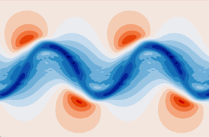
where, as before,  $L=2{\rm \pi}$ denotes the extent of the domain. We use the Fourier transform of (4.4), $u_{\boldsymbol {k}}$, plus a small sinusoidal perturbation in the corresponding $h_{\boldsymbol {k}}$ from $h \sim \sin (10 {\rm \pi}x/L$) to form the state vector $\boldsymbol {z}=(u_{\boldsymbol {k}},0,h_{\boldsymbol {k}})$. The corresponding sinusoidal perturbation in $v$ is chosen to be approximately $10^{-5}$ times smaller than the jet-like flow in $u$. As before, we obtain the base point by projecting $\boldsymbol {z}$ on the geostrophic mode, i.e. $\boldsymbol {z}_*^0 = \mathbb {P}_{\boldsymbol {k}}^0 \boldsymbol {z}$ (again, with the projector chosen to be compatible with the numerical scheme in use). The amplitude of $\boldsymbol {z}_*^0$ is then scaled to yield a maximum jet speed of $u=1.4$, which finally yields $\boldsymbol {z}_{{\textit {jet}}}$. Figure 2(a–c) shows the resulting jet-like balanced initial condition $\boldsymbol {z}_{{\textit {jet}}} + B_{4}(\boldsymbol {z}_{{\textit {jet}}})$ in the finite difference model for ${\textit {Ro}}=0.1$. Both models are integrated from $t=0$ to $t=t'=4/{\textit {Ro}}$ where the imbalance $I$ is diagnosed. Here, we choose a larger $t'$ compared with the random field configuration to allow the flow to fully develop its instability where it may emit waves. The fully developed instability can be seen in figure 2(d–f) for the finite difference model, the fields for the spectral model and using different balancing methods are again visually very similar.
As in figure 1, but for the jet flow initialization  $\boldsymbol {z}_{{\textit {jet}}} + B_4(\boldsymbol {z}_{{\textit {jet}}})$ in the finite difference model for ${\textit {Ro}}=0.1$. We show the fields at $t=0$ (a–c) and the evolved state at $t'=4/{\textit {Ro}}$ (d–f).

5. Results
In this section, we discuss the performance of the two balancing methods – higher order ( $B_1,\ldots, B_4$) and optimal balance ( $B_{{\textit {opt}}}$) – in the two different models – the spectral (SPEC) and finite difference (DIFF) discretizations – using the two different balanced initial conditions – random ( $\boldsymbol {z}_{{\textit {rand}}}$) and jet-like ( $\boldsymbol {z}_{{\textit {jet}}}$). In general, the diagnosed imbalance or residual wave signal is very small in both models, for both initial conditions. We therefore detect no significant wave emission in any of the experiments discussed here in agreement with the results of Chouksey et al. (Reference Chouksey, Eden and Olbers2022). However, we shall describe and discuss small differences in performance which are particularly visible in the jet-like test case.
5.1. Random initial conditions
Figure 3 shows the diagnosed imbalance in DIFF for  $\boldsymbol {z}_{{\textit {rand}}}$ using $B_n$ for different orders $n$. The residual wave signal scales as expected for $B_0$ to $B_2$, i.e. as ${\textit {Ro}}$ for $B_0$, as ${\textit {Ro}}^2$ for $B_1$ and as ${\textit {Ro}}^3$ for $B_2$. For $B_3$ and $B_4$, the expected scaling is only seen for small Rossby numbers. In fact, for ${\textit {Ro}}$ getting close to $1$, the residuals start growing when the order is increased. It is difficult to judge if this behaviour is due to actual gravity wave emission, imperfection of our implementation of the method, an already diverging power series or numerical truncation errors. We expect that for ${\textit {Ro}}$ approaching $1$, the optimal truncation is of rather low order so that the quality of balance decreases when including higher-order terms, as seen in figure 3. However, we noticed that small details in the numerical coding affect the residual drastically (not shown), as already noted by Eden et al. (Reference Eden, Chouksey and Olbers2019a), pointing towards a large role of numerical truncation errors.
Diagnosed imbalance  $I(\boldsymbol {u})$ (a) and $I(h)$ (b) in DIFF using the field $\boldsymbol {z}_{{\textit {rand}}}$ balanced with $B_4$ (black), $B_3$ (green), $B_2$ (magenta), $B_1$ (red) and $B_0$ (orange), as a function of Rossby number ${\textit {Ro}}$. The thin black lines denote different scaling laws, i.e. ${\textit {Ro}}^2$ (dotted), ${\textit {Ro}}^3$ (dashed) and ${\textit {Ro}}^4$ (dashed-dotted).

Figure 4 compares the performance of  $B_4$ and $B_{{\textit {opt}}}$ in SPEC and DIFF; $B_{{\textit {opt}}}$ scales in general similar to $B_4$ in all cases, but the overall level of the residuals can be different, although still very small in all cases. The residual wave signal is here slightly larger in SPEC than DIFF. However, using also $T=2$ for $B_{{\textit {opt}}}$ in DIFF, the residuals are getting very similar to $B_{{\textit {opt}}}$ in SPEC (not shown). The impact of ramp time $T$ on the diagnosed imbalanced is documented in Masur & Oliver (Reference Masur and Oliver2020) and not repeated here. For larger $T$, the residual gets smaller, but for even larger $T$, the residual increases again. The optimal $T$ for this configuration is between $T=2$ and $T=4$ for DIFF, but for SPEC the optimal $T$ is between $T=0.5$ and $T=2$. This points towards the importance of the numerics for the performance of the optimal balance method. Masur & Oliver (Reference Masur and Oliver2020) also discussed the impact of the threshold to terminate the iteration in $B_{{\textit {opt}}}$; they show that the impact is minor and the same is true here. The impact of the choice of the ramp function $\rho (\tau /T)$ is also documented in Masur & Oliver (Reference Masur and Oliver2020); here, we use the exponential ramp function given in (3.10), which is the optimal choice in Masur & Oliver (Reference Masur and Oliver2020).
Diagnosed imbalance  $I(\boldsymbol {u})$ (a) and $I(h)$ (b) using the field $\boldsymbol {z}_{{\textit {rand}}}$ balanced with $B_4$ in DIFF (black), $B_{{\textit {opt}}}$ in SPEC with $T=2$ (blue), $B_{{\textit {opt}}}$ in DIFF with $T=4$ (green) and $B_{{\textit {opt}}}$ in DIFF with $T=4$ but 10 times smaller time step (red). The thin black lines denote different scaling laws, i.e. ${\textit {Ro}}^2$ (dotted), ${\textit {Ro}}^3$ (dashed) and ${\textit {Ro}}^4$ (dashed-dotted). Dots denote individual experiments.

The diagnosed imbalance for DIFF using  $B_{{\textit {opt}}}$ with $T=4$ gets rather noisy at small ${\textit {Ro}}$ and fluctuates by orders of magnitude for small changes in ${\textit {Ro}}$. When decreasing the time step by a factor $10$, this behaviour disappears, the dependency of the diagnosed imbalance on ${\textit {Ro}}$ becomes smooth and the residuals get again smaller than with larger time step. An accurate time-stepping scheme appears therefore important for the performance of optimal balance, while this is not the case for $B_4$ (not shown). Reducing the time step further by an overall factor of $20$ reduces the residual only at very small ${\textit {Ro}}$ (not shown), so that for the parameter range shown, the results for $B_{{\textit {opt}}}$ are not affected by the accuracy of the time-stepping scheme and other errors appear to dominate.
Figure 5 shows the residual wave signal  $\boldsymbol {z}' - \boldsymbol {z}''$ after rebalancing at $t=0.5/{\textit {Ro}}$ for a fixed Rossby number ${\textit {Ro}}=0.1$ using $\boldsymbol {z}_{{\textit {rand}}}$, both models and balancing methods. For all cases, the residual shows in all variables a large-scale pattern, clearly deviating from geostrophic balance. We see no systematic difference for the different balancing methods in their spatial patterns, except for the different magnitude of the residual. However, the case using DIFF and $B_{{\textit {opt}}}$ with $T=4$ and smaller time step shows also noise on smaller scales which is not present for the other cases which have larger diagnosed imbalance. Using a time step $20$ times smaller, the noise remains the same, and also the diagnosed imbalance as mentioned before.
Residual wave signal  $\boldsymbol {z}' - \boldsymbol {z}''$ after rebalancing at $t=0.5/{\textit {Ro}}$ for ${\textit {Ro}}=0.1$ and $\boldsymbol {z}_{{\textit {rand}}}$ in DIFF and $B_4$ (a), in SPEC and $B_{{\textit {opt}}}$ with $T=2$ (b) and in DIFF and $B_{{\textit {opt}}}$ with $T=4$ and 10 times smaller time step (c). We show $h/{\textit {Ro}}^4$ in colour and $u$,
$u$,  $v$ as arrows, with magnitude of $O(10^{-6})$.

5.2. Jet-like initial conditions
Figure 6 shows the diagnosed imbalance of both methods in both models using the jet-like initial conditions instead of the random case. Here,  $B_4$ scales roughly as ${\textit {Ro}}^4$, similar to the case using $\boldsymbol {z}_{{\textit {rand}}}$, pointing again to numerical truncation errors for the highest orders; $B_{{\textit {opt}}}$ scales shallower, but shows smaller residuals for ${\textit {Ro}}>0.1$ than $B_4$ and $B_{{\textit {opt}}}$ in DIFF depends again on the quality of the time-stepping method, i.e. the fluctuations of the diagnosed imbalance for only small changes in ${\textit {Ro}}$ seen at small ${\textit {Ro}}<0.1$ for the normal time step disappear using a 20 times smaller time step. Also, $B_{{\textit {opt}}}$ in SPEC has smaller residuals than $B_{{\textit {opt}}}$ in DIFF for ${\textit {Ro}}<0.1$ in $I(h)$, but larger residuals than $B_{{\textit {opt}}}$ in DIFF for ${\textit {Ro}}<0.1$ in $I(\boldsymbol {u})$, while they are similar for ${\textit {Ro}}>0.1$. This shows that, at the level of the very small residuals, the different model codes can better reduce the residuals in different variables, and points again to the large role of numerical details and different errors for the quality of the balancing methods.
Diagnosed imbalance  $I(\boldsymbol {u})$ (a) and $I(h)$ (b) for $\boldsymbol {z}_{{\textit {jet}}}$ in DIFF balanced with $B_4$ (black), in SPEC using $B_{{\textit {opt}}}$ with $T=4$ (blue), in DIFF using $B_{{\textit {opt}}}$ with $T=4$ (green) and in DIFF using $B_{{\textit {opt}}}$ with $T=4$ but 20 times smaller time step (red). The thin black lines denote different scaling laws, i.e. ${\textit {Ro}}^2$ (dotted), ${\textit {Ro}}^3$ (dashed) and ${\textit {Ro}}^4$ (dashed-dotted). Dots denote individual experiments.

Figure 7 shows the residual wave signal for  ${\textit {Ro}}=0.1$ for the different balancing methods and numerical models using $\boldsymbol {z}_{{\textit {jet}}}$. While the residuals in DIFF are on the same scale as the jet, the very small residual in $h$ using $B_{{\textit {opt}}}$ in SPEC begins to show smaller scales similar to what has been reported before as gravity wave emission during frontogenesis (e.g. Plougonven & Snyder Reference Plougonven and Snyder2007). However, note the small magnitude of the signal, which is much different to the wave signal reported in the previous section for the random field case.
Residual wave signal  $\boldsymbol {z}'-\boldsymbol {z}''$ after rebalancing at $t=4/{\textit {Ro}}$ for ${\textit {Ro}}=0.1$ in DIFF for $\boldsymbol {z}_{{\textit {jet}}}$ using $B_4$ (a), in SPEC using $B_{{\textit {opt}}}$ with $T=4$ (b) and in DIFF using $B_{{\textit {opt}}}$ with $T=4$ and $20$ times smaller time step(c). We show $h/{\textit {Ro}}^4$ in colour and $u$,
$u$,  $v$ as arrows, with magnitude of $O(10^{-7})$.

5.3. Cross-balancing
In this section we discuss experiments where the imbalance  $I(\boldsymbol {u})$ and $I(h)$ of the balanced state from the one method is diagnosed with the other method, which we refer to as cross-balancing. Note that using any balanced state from SPEC in DIFF or vice versa introduces errors already at zero order in ${\textit {Ro}}$, because of the incompatible eigenvectors for the different numerical grids (A-grid vs C-grid). Figure 8 (green line) shows such a case, where the analytical eigenvectors $\boldsymbol {q}_k^\sigma$, $\boldsymbol {p}_k^\sigma$ appropriate for an A-grid instead of the corresponding ones for the C-grid are used for balancing with $B_4$. The error is large and does not change much for smaller ${\textit {Ro}}$. The spectral model behaves correspondingly. However, cross-balancing in the same numerical model with the same grid will provide additional information how the different (approximately) balanced states differ.
Diagnosed imbalance  $I(\boldsymbol {u})$ (a) and $I(h)$ (b) for $\boldsymbol {z}_{{\textit {rand}}}$ in DIFF using $B_4$ (black), $B_{{\textit {opt}}}$ with $T=4$ (blue) and the cross-balancing experiments using first $B_4$ then $B_{{\textit {opt}}}$ (green) and first $B_{{\textit {opt}}}$ then $B_4$ (red). The thin black lines denote different scaling laws, i.e. ${\textit {Ro}}^2$ (dotted), ${\textit {Ro}}^3$ (dashed) and ${\textit {Ro}}^4$ (dashed-dotted). Also shown is a case with $B_4$ in DIFF (orange), where the eigenvectors for the A-grid are used instead of the correct ones.

First, we balance DIFF using  $\boldsymbol {z}_{{\textit {rand}}}$ at $t=0$ with $B_4$, then we integrate to $t=0.5/{\textit {Ro}}$ and rebalance with $B_{{\textit {opt}}}$ (using $T=4$) and diagnose the imbalance from the difference to the state at $t=0.5/{\textit {Ro}}$ (shown as yellow line in figure 8). Second, we initially balance with $B_{{\textit {opt}}}$ (using $T=4$) and rebalance later with $B_4$ and diagnose the imbalance (shown as red line in figure 8). In both cases, the resulting diagnosed imbalance is only slightly larger than or almost equal to the maximum of $I(\boldsymbol {u})$ or $I(h)$ of the corresponding experiments using either $B_{{\textit {opt}}}$ or $B_4$ only. Thus, we conclude that both methods find a similar (approximately) balanced state.
6. Discussion and conclusions
In this study, we compare two different methods to approximately balance geophysical flows: the higher-order asymptotic implementation inspired by Warn et al. (Reference Warn, Bokhove, Shepherd and Vallis1995) and the optimal balance implementation of Masur & Oliver (Reference Masur and Oliver2020). We use here a single-layer shallow water model as example, but both methods can also readily be applied in three-dimensional models. We show that both methods can be understood as adding to the linear geostrophic mode  $\boldsymbol {z}_0$ contributions $B_n(\boldsymbol {z}_0)$ and $B_{{\textit {opt}}}(\boldsymbol {z}_0)$, respectively, taken from the linear wave modes, the so-called slaved modes, to generate a balanced state which evolves only slowly in time in the nonlinear model.
The main finding of this paper is that optimal balance and fourth-order in Rossby-number asymptotics can be considered equivalent for practical purposes. The residual wave signals of both balancing methods are comparable and show similar spatial patterns. There are, however, differences in the magnitude of the diagnosed imbalance for different model codes and initial conditions. It is difficult to decide if these differences are due to numerical issues such as truncation error or errors introduced by the time-stepping scheme, or systematic. Cross-balancing, i.e. balancing the model with one method and diagnosing the imbalance with the other one, suggests that both methods find approximately the same balanced states.
It has long been known that the quality of preservation of balance might depend on the numerical scheme (see, e.g. Mohebalhojeh & Dritschel Reference Mohebalhojeh and Dritschel2000). Here, we are able to show that adapting the notion of balance when changing between the finite difference and the spectral scheme yields comparably very good preservation of balance. It is only when mixing notions of balance across schemes that quality of preservation of balance drops. For more practical applications, such as defining balance for observational data, this implies that for a single-time snapshot of observational data the leading-order balance is as good (or bad) as higher-order balance. To increase the accuracy for the splitting of observational data into balanced and imbalanced motion, the only way is to use temporal-spatial data with a data assimilation scheme which includes a higher-order characterization of balance that matches the numerical model.
A practical difference between the balancing methods presented here is the computing resource demand. While the higher-order balance method only needs to run the model for a few time steps at maximum, followed by a few (fast) Fourier transforms, the optimal balance method needs to integrate the model over a sufficiently long ramping time, which needs significantly more computing resources. On the other hand, the optimal balance model appears easier to implement for a given numerical code.
Our results are presented in terms of the ‘diagnosed imbalance’ which picks up contributions that could be either due to imperfections of the balancing method or due to actual wave emission of the balanced flow. We find that the diagnosed imbalance, thus both contributing signals, decay rapidly with decreasing Rossby number. This implies, in particular that spontaneous emission of gravity waves is negligible in flows within typical geophysical parameters, in agreement with much earlier work such as Dritschel & Viúdez (Reference Dritschel and Viúdez2007) or Chouksey et al. (Reference Chouksey, Eden and Olbers2022) who found significant wave emission during balanced shear flow instabilities in a three-dimensional flow only if symmetric or convective instabilities occur and the Rossby number is close to unity. This conclusion is of practical relevance since several studies have previously reported significant spontaneous wave emission by balanced flow (e.g. Plougonven & Snyder Reference Plougonven and Snyder2007; Borchert, Achatz & Fruman Reference Borchert, Achatz and Fruman2014), which is also proposed as a significant sink of meso-scale eddy energy in the ocean based on global estimates from laboratory experiments (Williams et al. Reference Williams, Haine and Read2008) and idealized numerical simulations (Brüggemann & Eden Reference Brüggemann and Eden2015; Sugimoto & Plougonven Reference Sugimoto and Plougonven2016). It is possible that the signals in those experiments are dominated by slaved modes rather than actual wave emission, which calls for re-evaluation of the experiments with the high-order methods available now. It is, however, outside of the scope of the present study to answer this issue.
There are two more obvious questions that also lie outside of the scope of this paper. First, none of our results is directly applicable to the original OPV formulation of Viúdez & Dritschel (Reference Viúdez and Dritschel2004) and it would be interesting to benchmark their scheme in comparison with others. However, this raises a new dimension of issues because, for a given resolution of the Eulerian grid, the effective resolution of the contour-advective semi-Lagrangian (CASL) scheme used in OPV balance is much higher, and so is the computational cost. Thus, we choose to focus on balancing schemes that appear best suited for future application to operational implementations of full atmosphere and ocean models.
Second, our current model setting is highly idealized. Other studies have explored more complex settings for wave-vortex decomposition, such as McIntyre & Norton (Reference McIntyre and Norton2000) using potential vorticity inversion, Mohebalhojeh & Dritschel (Reference Mohebalhojeh and Dritschel2000) and Mirzaei, Mohebalhojeh & Ahmadi-Givi (Reference Mirzaei, Mohebalhojeh and Ahmadi-Givi2012) using the CASL and diabatic-CASL schemes, respectively, and Chouksey et al. (Reference Chouksey, Eden and Brüggemann2018), Eden et al. (Reference Eden, Chouksey and Olbers2019a) and Chouksey et al. (Reference Chouksey, Eden and Olbers2022) extending first-order (Machenhauer Reference Machenhauer1977) to higher-order balance of Warn et al. (Reference Warn, Bokhove, Shepherd and Vallis1995) for a range of flow regimes. We conjecture that both methods analysed here are good candidates for computing high-accuracy balance in these and other circumstances. However, one common obstacle is that a spectral transform is necessary to project on the linear geostrophic mode, which is difficult to implement in non-trivial cases. We are currently working to resolve this issue, with the goal to apply the optimal balance method to realistic ocean models which will offer a variety of interesting practical applications of the method.
Acknowledgements
We thank the referees for their extremely detailed and constructive reviews which helped to considerably improve the manuscript.
Funding
This paper is a contribution to subprojects W2, L2 and W6 of the Collaborative Research Centre TRR 181 ‘Energy Transfers in Atmosphere and Ocean’ funded by the Deutsche Forschungsgemeinschaft (DFG, German Research Foundation) under project number 274762653. G.T.M. is also supported through the Collaborative Research Center TRR 301 ‘The Tropopause Region in a Changing Atmosphere’ funded by DFG under project number 428312742.
Declaration of interests
The authors report no conflict of interest.


 Open access

