


1. Introduction
Particle-laden horizontal pipe flows are widely encountered in numerous applications and environmental contexts, leading to a renewed focus on the fundamental aspects of these flows over the recent past (e.g. Balachandar & Eaton Reference Balachandar and Eaton2010; Brandt & Coletti Reference Brandt and Coletti2022). Unladen canonical turbulent wall-bounded flow (such as pipes, say of diameter $D$
, channels and flat-plate boundary layers) can be characterised by Reynolds number alone, which for a pipe is either the bulk Reynolds number
$D$
, channels and flat-plate boundary layers) can be characterised by Reynolds number alone, which for a pipe is either the bulk Reynolds number $Re_b=u_b D/\nu$
or the friction Reynolds number
$Re_b=u_b D/\nu$
or the friction Reynolds number $Re_\tau =u_\tau R/\nu$
, where
$Re_\tau =u_\tau R/\nu$
, where $u_b$
is the bulk velocity,
$u_b$
is the bulk velocity, $u_{\tau }$
and
$u_{\tau }$
and $\nu$
are respectively the wall friction velocity and kinematic viscosity of the fluid, and the radius is
$\nu$
are respectively the wall friction velocity and kinematic viscosity of the fluid, and the radius is $R=D/2$
. Inclusion of particles, say spherical ones of diameter
$R=D/2$
. Inclusion of particles, say spherical ones of diameter $d_p$
and density
$d_p$
and density $\rho _p$
, into the flow leads to two additional non-dimensional groups: the viscous Stokes number
$\rho _p$
, into the flow leads to two additional non-dimensional groups: the viscous Stokes number $St^+=\tau _{p} / \tau _{f,\nu }$
, where
$St^+=\tau _{p} / \tau _{f,\nu }$
, where $\tau _{p} = d_{p}^{2}\rho _{p}/(18\nu \rho _{f})$
is the particle relaxation time (with
$\tau _{p} = d_{p}^{2}\rho _{p}/(18\nu \rho _{f})$
is the particle relaxation time (with $\rho _f$
the fluid density), and
$\rho _f$
the fluid density), and $\tau _{f,\nu } = \nu /u_{\tau }^{2}$
is the fluid viscous time scale, and the density ratio
$\tau _{f,\nu } = \nu /u_{\tau }^{2}$
is the fluid viscous time scale, and the density ratio $\rho _p/\rho _f$
. Since the amount of particle loading is also important, the volume fraction of the particles
$\rho _p/\rho _f$
. Since the amount of particle loading is also important, the volume fraction of the particles $\phi _v$
(or the mass fraction) is also a non-dimensional group. Consequently, particle-laden pipe flows could be described by four non-dimensional groups:
$\phi _v$
(or the mass fraction) is also a non-dimensional group. Consequently, particle-laden pipe flows could be described by four non-dimensional groups: $St^+$
,
$St^+$
, $\rho _p/\rho _f$
,
$\rho _p/\rho _f$
, $\phi _v$
and
$\phi _v$
and $Re_\tau = (R/u_\tau )/\tau _{f,\nu }$
, where
$Re_\tau = (R/u_\tau )/\tau _{f,\nu }$
, where $Re_\tau$
is written as a ratio of outer inertial and inner viscous time scales to complement the
$Re_\tau$
is written as a ratio of outer inertial and inner viscous time scales to complement the $St^+$
definition. Note that in applications where buoyancy forces owing to gravitational acceleration
$St^+$
definition. Note that in applications where buoyancy forces owing to gravitational acceleration $g$
on the particles are important,
$g$
on the particles are important, $g^{\prime}\equiv (\rho _p/\rho _f-1)g$
is a relevant quantity, hence the non-dimensional group
$g^{\prime}\equiv (\rho _p/\rho _f-1)g$
is a relevant quantity, hence the non-dimensional group $\rho _p/\rho _f$
(or
$\rho _p/\rho _f$
(or $St^+$
) is sometimes replaced by
$St^+$
) is sometimes replaced by $g^+ = g^{\prime}/(u_\tau ^3/\nu )$
or Shield number
$g^+ = g^{\prime}/(u_\tau ^3/\nu )$
or Shield number $Sh = (u_\tau ^2/{d}_p)/g^{\prime}$
in the context of wall-turbulence, or by Galileo number
$Sh = (u_\tau ^2/{d}_p)/g^{\prime}$
in the context of wall-turbulence, or by Galileo number $Ga = \sqrt {g^{\prime}/(\nu ^2/d_p^3)}$
in more general scenarios. In applications with solid or liquid particles in air,
$Ga = \sqrt {g^{\prime}/(\nu ^2/d_p^3)}$
in more general scenarios. In applications with solid or liquid particles in air, $\rho _p/\rho _f = O(1000)$
, whereas particles in water result in
$\rho _p/\rho _f = O(1000)$
, whereas particles in water result in $\rho _p/\rho _f = O(1)$
. Another factor (apart from the four non-dimensional groups) in wall flows is the relative directions of mean flow and gravity, whether they are aligned or perpendicular to each other, and results in vertical and horizontal flow set-ups. A consequence of this expansive parameter space is that a large body of work is required to obtain a comprehensive understanding of particle-laden flows.
$\rho _p/\rho _f = O(1)$
. Another factor (apart from the four non-dimensional groups) in wall flows is the relative directions of mean flow and gravity, whether they are aligned or perpendicular to each other, and results in vertical and horizontal flow set-ups. A consequence of this expansive parameter space is that a large body of work is required to obtain a comprehensive understanding of particle-laden flows.
The focus of the present experimental work is on particles in water (i.e. $\rho _p/\rho _f = O(1)$
) in a horizontal pipe, where
$\rho _p/\rho _f = O(1)$
) in a horizontal pipe, where $Re_\tau \approx 195$
is nominally constant, and
$Re_\tau \approx 195$
is nominally constant, and $St^+$
(
$St^+$
( $\approx 1$
–
$\approx 1$
– $4$
) and
$4$
) and $\phi _v$
(
$\phi _v$
( $0.25{-}1\,\%$
) are such that we are in the two-way coupling regime (i.e. particle–fluid interaction can change the mean and turbulence statistics of the background fluid). especially important in horizontal pipes where even a small increase in
$0.25{-}1\,\%$
) are such that we are in the two-way coupling regime (i.e. particle–fluid interaction can change the mean and turbulence statistics of the background fluid). especially important in horizontal pipes where even a small increase in $\rho _p/\rho _f$
variation on the mean and turbulence statistics of fluid and particles. This is especially important in horizontal pipes where even a small increase in
$\rho _p/\rho _f$
variation on the mean and turbulence statistics of fluid and particles. This is especially important in horizontal pipes where even a small increase in $\rho _p/\rho _f$
of approximately
$\rho _p/\rho _f$
of approximately $O(1)$
can lead to particle settling. It is quite common among experimental investigations of water flow to take
$O(1)$
can lead to particle settling. It is quite common among experimental investigations of water flow to take $\rho _p/\rho _f$
close to unity; however, rarely do we have
$\rho _p/\rho _f$
close to unity; however, rarely do we have $\rho _p/\rho _f=1$
, because of limitations in finding particles with densities similar to water in large quantities, or applications require
$\rho _p/\rho _f=1$
, because of limitations in finding particles with densities similar to water in large quantities, or applications require $\rho _p/\rho _f\approx 1$
but not unity. A sample of experimental investigations (in both vertical and horizontal pipes, channels and boundary layers) are listed in table 1, where in most investigations
$\rho _p/\rho _f\approx 1$
but not unity. A sample of experimental investigations (in both vertical and horizontal pipes, channels and boundary layers) are listed in table 1, where in most investigations $\rho _p/\rho _f$
is close to unity (within 1.6–5 %) but not close enough to 1 (except in the numerical simulations of Picano et al. (Reference Picano, Breugem and Brandt2015)). It would perhaps seem that the turbulence characteristics of particle-laden flows with such small variations in density ratios would be similar to the neutrally buoyant particle case. In fact, most experiments in horizontal flows (e.g. Ahmadi et al. Reference Ahmadi, Ebrahimian, Sanders and Ghaemi2019) show an increase in vertical or radial fluid turbulence intensity with an addition of particles, whereas some show an increase in axial turbulence intensity, but others (e.g. Kaftori et al. Reference Kaftori, Hetsroni and Banerjee1995; Kiger & Pan Reference Kiger and Pan2002; Nezu & Azuma Reference Nezu and Azuma2004; Righetti & Romano Reference Righetti and Romano2004) show no substantial change. Shear stress also appears to increase relative to the unladen flow case (e.g. Shokri et al. Reference Shokri, Ghaemi, Nobes and Sanders2017). Note that Baker & Coletti (Reference Baker and Coletti2021) observe particle settling even with 1.6 % density difference between particles and the fluid. Furthermore, there is little information on the effects on the mean flow, i.e. any drag increase or decrease. The notable exception is the direct numerical simulations (DNS) of Picano, Breugem & Brandt (Reference Picano, Breugem and Brandt2015), who (although with a larger
$\rho _p/\rho _f$
is close to unity (within 1.6–5 %) but not close enough to 1 (except in the numerical simulations of Picano et al. (Reference Picano, Breugem and Brandt2015)). It would perhaps seem that the turbulence characteristics of particle-laden flows with such small variations in density ratios would be similar to the neutrally buoyant particle case. In fact, most experiments in horizontal flows (e.g. Ahmadi et al. Reference Ahmadi, Ebrahimian, Sanders and Ghaemi2019) show an increase in vertical or radial fluid turbulence intensity with an addition of particles, whereas some show an increase in axial turbulence intensity, but others (e.g. Kaftori et al. Reference Kaftori, Hetsroni and Banerjee1995; Kiger & Pan Reference Kiger and Pan2002; Nezu & Azuma Reference Nezu and Azuma2004; Righetti & Romano Reference Righetti and Romano2004) show no substantial change. Shear stress also appears to increase relative to the unladen flow case (e.g. Shokri et al. Reference Shokri, Ghaemi, Nobes and Sanders2017). Note that Baker & Coletti (Reference Baker and Coletti2021) observe particle settling even with 1.6 % density difference between particles and the fluid. Furthermore, there is little information on the effects on the mean flow, i.e. any drag increase or decrease. The notable exception is the direct numerical simulations (DNS) of Picano, Breugem & Brandt (Reference Picano, Breugem and Brandt2015), who (although with a larger $\phi _v$
ranging from
$\phi _v$
ranging from $5\,\%$
to
$5\,\%$
to $20\,\%$
) fix
$20\,\%$
) fix $\rho _p/\rho _f = 1$
, and find an overall drag increase. Interestingly, they report a reduction in all turbulent stresses compared to an unladen flow, which seems opposite to the limited experimental observations. Note that as table 1 shows, even the smallest
$\rho _p/\rho _f = 1$
, and find an overall drag increase. Interestingly, they report a reduction in all turbulent stresses compared to an unladen flow, which seems opposite to the limited experimental observations. Note that as table 1 shows, even the smallest $\phi _v=5\,\%$
used in DNS is not an easy case for experiments using laser-based techniques because of the blocking effects caused by the particles.
$\phi _v=5\,\%$
used in DNS is not an easy case for experiments using laser-based techniques because of the blocking effects caused by the particles.
A list of numerical and experimental studies investigating wall-bounded particle-laden flows. The parameters are derived by utilising the data provided within references when they are not explicitly stated in the papers. Here, $Re_{\tau }$
and
$Re_{\tau }$
and $d_{p}^+$
are friction Reynolds number and mean particle diameter in wall units, respectively. In the second column, the abbreviations ‘Expt’, ‘Ch’, ‘pipe’, BL indicate the experiments in channel, pipe and boundary layer, whereas ‘H’ and ‘V’ mean horizontal and vertical, respectively. For example, ‘H-Pipe(Expt)’ indicates the experimental study in a horizontal pipe.
$d_{p}^+$
are friction Reynolds number and mean particle diameter in wall units, respectively. In the second column, the abbreviations ‘Expt’, ‘Ch’, ‘pipe’, BL indicate the experiments in channel, pipe and boundary layer, whereas ‘H’ and ‘V’ mean horizontal and vertical, respectively. For example, ‘H-Pipe(Expt)’ indicates the experimental study in a horizontal pipe.

The objective of the present experimental investigation is to carry out time-resolved two-phase flow experiments in a horizontal pipe with $\rho _p/\rho _f = 1.05$
and
$\rho _p/\rho _f = 1.05$
and $\rho _p/\rho _f = 1$
(or close to 1 by increasing the density of the fluid to match the particles), and study the effects on the mean and turbulent stresses of fluid and particle phase. We also present two-point spatial correlation and fluid spectra to explore the effect of density ratio on the size of turbulent structures. We see clear differences in turbulent statistics and the length scale of turbulence for the variation in density ratio, primarily because of a small but significant settling velocity for
$\rho _p/\rho _f = 1$
(or close to 1 by increasing the density of the fluid to match the particles), and study the effects on the mean and turbulent stresses of fluid and particle phase. We also present two-point spatial correlation and fluid spectra to explore the effect of density ratio on the size of turbulent structures. We see clear differences in turbulent statistics and the length scale of turbulence for the variation in density ratio, primarily because of a small but significant settling velocity for $\rho _p/\rho _f = 1.05$
. We also vary
$\rho _p/\rho _f = 1.05$
. We also vary $\phi _v$
and
$\phi _v$
and $St^+$
for the two density ratios. Planar laser-based imaging techniques of particle image and tracking velocimetry (PIV and PTV) are employed to document the dynamics of fluid and particle phases separately. The rest of the paper is organised as follows. The experimental facility and measurement methodology are introduced in § 2. Next, the comparisons of fluid and particle velocity statistics for
$St^+$
for the two density ratios. Planar laser-based imaging techniques of particle image and tracking velocimetry (PIV and PTV) are employed to document the dynamics of fluid and particle phases separately. The rest of the paper is organised as follows. The experimental facility and measurement methodology are introduced in § 2. Next, the comparisons of fluid and particle velocity statistics for $\rho _p/\rho _f=1$
and 1.05 are presented respectively in §§ 3 and 4. Since particles settle vertically, instantaneous vertical velocity fields and their probability density functions for the two density ratios are discussed in § 5. Effects on the turbulent length scales are explored in § 6 using two-point correlations and velocity spectra, and finally, the paper is summarised and concluded in § 7.
$\rho _p/\rho _f=1$
and 1.05 are presented respectively in §§ 3 and 4. Since particles settle vertically, instantaneous vertical velocity fields and their probability density functions for the two density ratios are discussed in § 5. Effects on the turbulent length scales are explored in § 6 using two-point correlations and velocity spectra, and finally, the paper is summarised and concluded in § 7.
2. Experimental set-up and validation
Experiments are conducted in a gravity-driven horizontal pipe of total length $L=4.3$
m and inner diameter
$L=4.3$
m and inner diameter $D=20.5$
mm, as depicted in figure 1. Measurements are carried out at a distance 3.91 m (
$D=20.5$
mm, as depicted in figure 1. Measurements are carried out at a distance 3.91 m ( $\approx 190D$
) from the pipe inlet. The set-up involves a recirculating water loop fed by gravity at a constant head. A pump recycles the outflow back to the header tank, and an overflow is applied to ensure a constant pressure head. The flow conditioning section consists of an expansion and a contraction with a honeycomb employed to straighten inflow at the pipe inlet. A fine-sand ring with uniform diameter
$\approx 190D$
) from the pipe inlet. The set-up involves a recirculating water loop fed by gravity at a constant head. A pump recycles the outflow back to the header tank, and an overflow is applied to ensure a constant pressure head. The flow conditioning section consists of an expansion and a contraction with a honeycomb employed to straighten inflow at the pipe inlet. A fine-sand ring with uniform diameter $60 \mathrm {\,\unicode{x03BC} m}$
is glued inside the pipe to trip the flow. A fully developed turbulent pipe flow is reasonably ensured with the measurement region located
$60 \mathrm {\,\unicode{x03BC} m}$
is glued inside the pipe to trip the flow. A fully developed turbulent pipe flow is reasonably ensured with the measurement region located $190D$
downstream of the entrance section. At the measurement location, a fully transparent water-filled rectangular acrylic section is placed around the pipe to minimise optical distortion in PIV imaging owing to pipe curvature. Additionally, acrylic self-adhesive black foils are used to reduce the background illumination and mitigate the laser-light reflection. The pressure measurement system includes an Omega Digital Panel DP32Pt and the Pressure Transducer PX 419-10DWU5V. The pressure transducer is calibrated to offset the impacts of thermal changes and sensitivity. Here, this pressure gradient
$190D$
downstream of the entrance section. At the measurement location, a fully transparent water-filled rectangular acrylic section is placed around the pipe to minimise optical distortion in PIV imaging owing to pipe curvature. Additionally, acrylic self-adhesive black foils are used to reduce the background illumination and mitigate the laser-light reflection. The pressure measurement system includes an Omega Digital Panel DP32Pt and the Pressure Transducer PX 419-10DWU5V. The pressure transducer is calibrated to offset the impacts of thermal changes and sensitivity. Here, this pressure gradient $\mathrm { d}P/\mathrm { d}x$
is used to estimate
$\mathrm { d}P/\mathrm { d}x$
is used to estimate $ u_\tau = \sqrt {(\mathrm { d}P/\mathrm { d}x) \, R / (2\rho _f) }$
. Discharge is measured by collecting the water on a digital weight scale, and temperature is monitored for each experiment. The quality of measurements (including those of density, dynamic viscosity, discharge and pressure) in a particle-free turbulent smooth pipe flow is ensured by comparing the results with the Moody diagram and existing DNS database (discussed in §§ 2.4 and 2.5).
$ u_\tau = \sqrt {(\mathrm { d}P/\mathrm { d}x) \, R / (2\rho _f) }$
. Discharge is measured by collecting the water on a digital weight scale, and temperature is monitored for each experiment. The quality of measurements (including those of density, dynamic viscosity, discharge and pressure) in a particle-free turbulent smooth pipe flow is ensured by comparing the results with the Moody diagram and existing DNS database (discussed in §§ 2.4 and 2.5).
Schematic of the experimental set-up.

2.1. Inertial particles and PIV fluorescent tracer
The inertial particles are injected into the pipe through a magnetic mixer and precision peristaltic pump (Lead Fluid YZ15), which is calibrated for the current experimental conditions. To distinguish the fluid and solid phases, in-house fluorescent tracer is produced, which consists of Rhodamine 6G and epoxy (Pedocchi, Martin & García Reference Pedocchi, Martin and García2008). Mastersizer 3000 manufactured by Malvern Panalytical is employed to analyse the density and size distribution of fluorescent tracer. The probability density function (PDF) and cumulative fraction of particles are as shown in figures 16(a) and 16(b), respectively, in Appendix A, and they show that the mean diameter and size distribution (D50) are respectively 30.3 $\mathrm {\,\unicode{x03BC} m}$
and 26.1
$\mathrm {\,\unicode{x03BC} m}$
and 26.1 $\mathrm {\,\unicode{x03BC} m}$
, corresponding to
$\mathrm {\,\unicode{x03BC} m}$
, corresponding to $St^+= 0.018$
(based on the mean diameter), which suggests that PIV particles follow the fluid reasonably well.
$St^+= 0.018$
(based on the mean diameter), which suggests that PIV particles follow the fluid reasonably well.
Polystyrene beads are chosen as the solid phase, and their density $\rho _p = 1050\,\mathrm {kg\,m^{-3}}$
is close to water but denser than water by approximately
$\rho _p = 1050\,\mathrm {kg\,m^{-3}}$
is close to water but denser than water by approximately $5\,\%$
. This means that in pure water, the beads will tend to gravitate towards the lower side of the wall. Two sets of polystyrene spherical beads from Maxi-Blast Inc. are utilised, with mean diameters
$5\,\%$
. This means that in pure water, the beads will tend to gravitate towards the lower side of the wall. Two sets of polystyrene spherical beads from Maxi-Blast Inc. are utilised, with mean diameters $d_{p} = 250\,\mathrm {\unicode{x03BC} m}$
and
$d_{p} = 250\,\mathrm {\unicode{x03BC} m}$
and $437\,\mathrm {\unicode{x03BC} m}$
, corresponding to ratios of the pipe diameter to the mean particle diameter
$437\,\mathrm {\unicode{x03BC} m}$
, corresponding to ratios of the pipe diameter to the mean particle diameter $D/d_{p}=82$
and 47, respectively. The size distributions of the small and large inertial particles are shown in figure 17 of Appendix B. Table 2 shows the relevant properties of fluorescent tracer and inertial particles at bulk velocity
$D/d_{p}=82$
and 47, respectively. The size distributions of the small and large inertial particles are shown in figure 17 of Appendix B. Table 2 shows the relevant properties of fluorescent tracer and inertial particles at bulk velocity $0.3\,\mathrm {m\,s^-}{^1}$
. Also, table 2 presents the approximate settling velocity
$0.3\,\mathrm {m\,s^-}{^1}$
. Also, table 2 presents the approximate settling velocity $u_{{ SV}}=(\rho _{p}-\rho _{f})g d_p^{2}/({18\mu })$
, which is obtained when the drag force equals the gravitational force in a stationary fluid. Notice that the large diameter particles result in larger
$u_{{ SV}}=(\rho _{p}-\rho _{f})g d_p^{2}/({18\mu })$
, which is obtained when the drag force equals the gravitational force in a stationary fluid. Notice that the large diameter particles result in larger $u_{{ SV}}$
.
$u_{{ SV}}$
.
Parameters of inertial particles and fluorescent tracers. The values of $St=\tau _p/(\nu /u_b^2)$
are at
$St=\tau _p/(\nu /u_b^2)$
are at $u_b=0.3\,{\rm m}\,{\rm s}^{-1}$
, which is the approximate value for most cases.
$u_b=0.3\,{\rm m}\,{\rm s}^{-1}$
, which is the approximate value for most cases.

Separate experiments are conducted to measure the velocities of the fluid and the inertial particles. For the fluid phase, we use the standard PIV technique seeded with the in-house fluorescent tracer. The fluorescent tracer illuminated by the green laser light and emitting red colour is captured by the PIV camera with a filter that allows only red colour (thus isolating the bright green light from the inertial particles). Separate experiments with only inertial particles (i.e. without fluorescent tracer) are also conducted with PTV to obtain velocity statistics of the inertial particles. In the following, we discuss first the PIV for fluid and then the PTV technique for the inertial particles.
2.2. Particle image velocimetry
For the continuous fluid phase, in-house fluorescent tracer is illuminated by an approximately 1 mm thick laser sheet by the Innolas Spitlight Compact Nd:YAG continuous laser with energy 10 mW and wavelength 532 nm. To record the instantaneous fluid and particle position separately, the experiment utilises a PCO Dimax HS high-speed camera (16-bit frame) with resolution $2000\times2000$
pixels, and 180 mm Tamron optical lenses in measurement area
$2000\times2000$
pixels, and 180 mm Tamron optical lenses in measurement area $25.2\times25.2$ $\mathrm {mm^2}$
. The high-speed camera is operated at 2000 Hz. In order to improve PIV accuracy and alleviate the effects of weak contrast between background and tracer, uneven tracer intensity, and high background intensity from some reflective objects, three pre-processing steps are carried out. First, the ensemble average of more than 1500 PIV images is extracted and subtracted from each image. Second, a low-pass filter is utilised to artificially enlarge the tracer size to alleviate the peak-locking bias. Finally, an upper-intensity histogram threshold approach is employed to mitigate the error from much stronger intensity. In total, each experiment recorded 76 140 raw PIV images that were processed by an in-house PIV package. This package has been tested for a variety of turbulent flow cases (e.g. Chauhan et al. Reference Chauhan, Philip, De Silva, Hutchins and Marusic2014; Kevin, Monty & Hutchins Reference Kevin, Monty and Hutchins2019; Setiawan, Philip & Monty Reference Setiawan, Philip and Monty2022). Its post-processing approach utilises deformation of the window and multi-grid to mitigate bias. Although the majority of inertial particles are filtered out by the band-pass filter, a few inertial particles illuminated by fluorescent light are still captured. To eliminate these particles, a Matlab program was applied to detect any stray inertial particles, which were removed before PIV analysis. Also, considering that the streamwise velocity is larger than the vertical one, we selected the interrogation window size
$\mathrm {mm^2}$
. The high-speed camera is operated at 2000 Hz. In order to improve PIV accuracy and alleviate the effects of weak contrast between background and tracer, uneven tracer intensity, and high background intensity from some reflective objects, three pre-processing steps are carried out. First, the ensemble average of more than 1500 PIV images is extracted and subtracted from each image. Second, a low-pass filter is utilised to artificially enlarge the tracer size to alleviate the peak-locking bias. Finally, an upper-intensity histogram threshold approach is employed to mitigate the error from much stronger intensity. In total, each experiment recorded 76 140 raw PIV images that were processed by an in-house PIV package. This package has been tested for a variety of turbulent flow cases (e.g. Chauhan et al. Reference Chauhan, Philip, De Silva, Hutchins and Marusic2014; Kevin, Monty & Hutchins Reference Kevin, Monty and Hutchins2019; Setiawan, Philip & Monty Reference Setiawan, Philip and Monty2022). Its post-processing approach utilises deformation of the window and multi-grid to mitigate bias. Although the majority of inertial particles are filtered out by the band-pass filter, a few inertial particles illuminated by fluorescent light are still captured. To eliminate these particles, a Matlab program was applied to detect any stray inertial particles, which were removed before PIV analysis. Also, considering that the streamwise velocity is larger than the vertical one, we selected the interrogation window size $64\times32$
pixels, with 50 % overlap.
$64\times32$
pixels, with 50 % overlap.
Particle detection: (a) particle image template (top left) and the detected particles; (b,c) examples of detected particles in the cases $\rho _p/\rho _f =1$
and
$\rho _p/\rho _f =1$
and $1.05$
, respectively.
$1.05$
, respectively.

2.3. Particle tracking technique
To acquire the velocities of inertial particles, experiments are performed with only inertial particles (i.e. no PIV tracers). An in-house Matlab code is developed to capture the particle positions, and subsequently obtain the velocity field by utilising two particle positions. To identify particles, the particle mask correlation algorithm introduced by Takehara & Etoh (Reference Takehara and Etoh1998) is employed by selecting a threshold value for binarisation, which assumes a particle image template, and searches in the observation area obtaining correlation of pixel intensity. To ensure accuracy, only correlation results larger than 0.8 are processed further. For example, figure 2(a) shows a raw image where the laser enters from the top, and we select a particle template with $45\times45$
pixels as shown in the top left. Then the three particles (shown by red circles) are detected after using a correlation algorithm. Figures 2(b) and 2(c) show an example each for
$45\times45$
pixels as shown in the top left. Then the three particles (shown by red circles) are detected after using a correlation algorithm. Figures 2(b) and 2(c) show an example each for $\rho _p/\rho _f =1$
and
$\rho _p/\rho _f =1$
and $1.05$
, respectively, where detected particles are shown by white filled circles.
$1.05$
, respectively, where detected particles are shown by white filled circles.
After identifying the spatial positions of particles, the cross-correlation method proposed by Hassan et al. (Reference Hassan, Blanchat, Seeley and Canaan1992) and Yamamoto et al. (Reference Yamamoto, Wada, Iguchi and Ishikawa1996) is employed on a processed image pair to calculate the velocity field. It is noted that the technique called binary cross-correlation is utilised since the particle images are recognised and binarised. In terms of the raw image pair, a circular area determined by centroid and radius in the first frame is applied to search in a potential moving area in the second frame. For example, assuming that the centre position is $(X,Y)$
in the first frame, and the radius of the particle was
$(X,Y)$
in the first frame, and the radius of the particle was $r$
pixels, the rectangle searching area was
$r$
pixels, the rectangle searching area was $(X-r,X+r+50)$
and
$(X-r,X+r+50)$
and $(Y-r-15,Y+r+15)$
. Here, 50 and 30 pixels are the potential maximum moving distances of the particle for a PIV image pair in streamwise and vertical directions. A pre-processing thresholding procedure is employed to remove out-of-focus inertial particles, and background subtraction from the ensemble average is performed to eliminate the fixed and strong reflections from the pipe wall.
$(Y-r-15,Y+r+15)$
. Here, 50 and 30 pixels are the potential maximum moving distances of the particle for a PIV image pair in streamwise and vertical directions. A pre-processing thresholding procedure is employed to remove out-of-focus inertial particles, and background subtraction from the ensemble average is performed to eliminate the fixed and strong reflections from the pipe wall.
Parameters of fluid and solid phases in the present experiments. For the buoyant cases of $\rho _p/\rho _f=1.05$
, the approximate volume fractions in the upper and lower halves of the pipe are shown in parentheses. For example, in case 3A,
$\rho _p/\rho _f=1.05$
, the approximate volume fractions in the upper and lower halves of the pipe are shown in parentheses. For example, in case 3A, $\phi _v=0.25\,\%$
is observed to be split up, respectively, as 0.18 % and 0.32 % in the upper and lower halves of the pipe. Here,
$\phi _v=0.25\,\%$
is observed to be split up, respectively, as 0.18 % and 0.32 % in the upper and lower halves of the pipe. Here, $u_{{ SV}}^+=u_{{ SV}}/u_\tau = (1/18)(Ga^2/d_p^+) = (1/18)(d_p^+/Sh) = (1/18)(d_p^{+2} g^+)$
,
$u_{{ SV}}^+=u_{{ SV}}/u_\tau = (1/18)(Ga^2/d_p^+) = (1/18)(d_p^+/Sh) = (1/18)(d_p^{+2} g^+)$
, $g^{\prime}\equiv (\rho _p/\rho _f-1)g$
,
$g^{\prime}\equiv (\rho _p/\rho _f-1)g$
, $Ga = \sqrt {g^{\prime}/(\nu ^2/d_p^3)}$
,
$Ga = \sqrt {g^{\prime}/(\nu ^2/d_p^3)}$
, $Sh = (u_\tau ^2/d_p)/g^{\prime}$
and
$Sh = (u_\tau ^2/d_p)/g^{\prime}$
and $g^+ = g^{\prime}/(u_\tau ^3/\nu )$
.
$g^+ = g^{\prime}/(u_\tau ^3/\nu )$
.

2.4. Experimental conditions
In this study, two particle volume fractions $\phi _v=0.25\,\%$
and
$\phi _v=0.25\,\%$
and $1 \pm 0.05\,\%$
are tested. The particles are fed into the pipe (before the inlet expansion) using a peristaltic pump at a metered flow rate from a known concentrated particle and water mixture placed on a digital scale. This allows us to estimate
$1 \pm 0.05\,\%$
are tested. The particles are fed into the pipe (before the inlet expansion) using a peristaltic pump at a metered flow rate from a known concentrated particle and water mixture placed on a digital scale. This allows us to estimate $\phi _v$
during the experiments. Furthermore, a sieve with aperture 63
$\phi _v$
during the experiments. Furthermore, a sieve with aperture 63 $\mathrm {\,\unicode{x03BC} m}$
(smaller than the particle diameter) is used to filter out the inertial particles, and a stopwatch is used to record the time duration. After measuring the weight of the dried particles,
$\mathrm {\,\unicode{x03BC} m}$
(smaller than the particle diameter) is used to filter out the inertial particles, and a stopwatch is used to record the time duration. After measuring the weight of the dried particles, $\phi _v$
is gain estimated, which is in reasonable agreement with the results from the PTV post-processing. As mentioned, for the solid phase velocity measurements, the experiments are performed with only inertial particles without any fluorescent tracer, whereas the fluid phase measurements include both inertial and PIV fluorescent particles. As such, separate experiments are run for measuring fluid and particle velocities.
$\phi _v$
is gain estimated, which is in reasonable agreement with the results from the PTV post-processing. As mentioned, for the solid phase velocity measurements, the experiments are performed with only inertial particles without any fluorescent tracer, whereas the fluid phase measurements include both inertial and PIV fluorescent particles. As such, separate experiments are run for measuring fluid and particle velocities.
Table 3 lists the parameters of all the particle-laden experiments. Case numbers 1 and 3 indicate the small inertial particle of diameter 250 $\mathrm {\,\unicode{x03BC} m}$
, respectively in neutrally buoyant (
$\mathrm {\,\unicode{x03BC} m}$
, respectively in neutrally buoyant ( $\rho _p/\rho _f=1.0$
) and buoyant (
$\rho _p/\rho _f=1.0$
) and buoyant ( $\rho _p/\rho _f=1.05$
) scenarios. Similarly, case numbers 2 and 4 indicate the large inertial particle of diameter 437
$\rho _p/\rho _f=1.05$
) scenarios. Similarly, case numbers 2 and 4 indicate the large inertial particle of diameter 437 $\mathrm {\,\unicode{x03BC} m}$
for the two different
$\mathrm {\,\unicode{x03BC} m}$
for the two different $\rho _p/\rho _f$
values. Also, a letter A or B indicates
$\rho _p/\rho _f$
values. Also, a letter A or B indicates $\phi _v$
at 0.25 % or 1 %. All the friction Reynolds numbers
$\phi _v$
at 0.25 % or 1 %. All the friction Reynolds numbers $Re_{\tau }$
are close to 195, and bulk Reynolds numbers (
$Re_{\tau }$
are close to 195, and bulk Reynolds numbers ( $Re_b = u_b D / \nu$
) are approximately 6000 corresponding to
$Re_b = u_b D / \nu$
) are approximately 6000 corresponding to $u_b\approx 0.30\,{\rm m}\,{\rm s}^{-1}$
. The current experiments span the range
$u_b\approx 0.30\,{\rm m}\,{\rm s}^{-1}$
. The current experiments span the range $St^+= 1.16{-}3.76$
. Table 3 also lists the ratio
$St^+= 1.16{-}3.76$
. Table 3 also lists the ratio $u_{b}/u_{\mathrm { SV}}$
, which shows that particles (in a still fluid) can settle vertically about a distance of
$u_{b}/u_{\mathrm { SV}}$
, which shows that particles (in a still fluid) can settle vertically about a distance of $D$
over pipe length
$D$
over pipe length $138D$
or
$138D$
or $50D$
, suggesting that settling of particles would be expected in our set-up. Also, we define a relevant non-dimensional viscous settling velocity
$50D$
, suggesting that settling of particles would be expected in our set-up. Also, we define a relevant non-dimensional viscous settling velocity $u_{{SV}}^+=u_{{SV}}/u_\tau$
that ranges from 0.12 to 0.32, and is not too small, indicating a different mechanism by which
$u_{{SV}}^+=u_{{SV}}/u_\tau$
that ranges from 0.12 to 0.32, and is not too small, indicating a different mechanism by which $\rho _p/\rho _f=1.05$
particles can interact with wall turbulence. For comparison with other works, table 3 presents parameters such as
$\rho _p/\rho _f=1.05$
particles can interact with wall turbulence. For comparison with other works, table 3 presents parameters such as $Ga$
,
$Ga$
, $Sh$
and
$Sh$
and $g^+$
. We note that in the channel experiments of Baker & Coletti (Reference Baker and Coletti2021),
$g^+$
. We note that in the channel experiments of Baker & Coletti (Reference Baker and Coletti2021), $Ga=11.3$
and
$Ga=11.3$
and $Sh=2$
for
$Sh=2$
for $\rho _p/\rho _f=1.016$
, whereas Lee & Lee (Reference Lee and Lee2019) in their numerical simulations take
$\rho _p/\rho _f=1.016$
, whereas Lee & Lee (Reference Lee and Lee2019) in their numerical simulations take $g^+=0.077$
at
$g^+=0.077$
at $\rho _p/\rho _f=833$
, and some of these parameters are within the range of our experiments with
$\rho _p/\rho _f=833$
, and some of these parameters are within the range of our experiments with $\rho _p/\rho _f=1.05$
. We will show that indeed some trends that we observe exhibit similarities to the results from the mentioned investigations.
$\rho _p/\rho _f=1.05$
. We will show that indeed some trends that we observe exhibit similarities to the results from the mentioned investigations.
Fresh water is the working fluid for $\rho _p/\rho _f=1.05$
, whereas water is made denser with salt to achieve the same fluid and particle density resulting in
$\rho _p/\rho _f=1.05$
, whereas water is made denser with salt to achieve the same fluid and particle density resulting in $\rho _p/\rho _f=1$
. The total acquisition time is
$\rho _p/\rho _f=1$
. The total acquisition time is $1114\,R/u_b$
, where
$1114\,R/u_b$
, where $R/u_b$
is the eddy turnover time. To achieve this total acquisition time, for each case, the images are captured in six separate batches (with each batch capturing 12 690 time-resolved images) owing to the maximum camera storage capacity. Appendix C shows the particle number densities for both
$R/u_b$
is the eddy turnover time. To achieve this total acquisition time, for each case, the images are captured in six separate batches (with each batch capturing 12 690 time-resolved images) owing to the maximum camera storage capacity. Appendix C shows the particle number densities for both $\rho _p/\rho _f=1$
and
$\rho _p/\rho _f=1$
and $1.05$
that are evaluated from the images. As expected,
$1.05$
that are evaluated from the images. As expected, $\rho _p/\rho _f=1.05$
shows a higher particle count at the bottom owing to settling, and although the
$\rho _p/\rho _f=1.05$
shows a higher particle count at the bottom owing to settling, and although the $\rho _p/\rho _f=1$
case shows a more uniform particle distribution for the upper and lower parts of the pipe, there is a slightly higher particle count for the lower half, and the likely reasons are suggested in Appendix C. To test the efficacy of achieving
$\rho _p/\rho _f=1$
case shows a more uniform particle distribution for the upper and lower parts of the pipe, there is a slightly higher particle count for the lower half, and the likely reasons are suggested in Appendix C. To test the efficacy of achieving $\rho _p/\rho _f=1$
in experiments, particles were suspended in a 10 cm high beaker of still salt water, and after approximately 10–20 min (for larger and smaller particles, respectively), some particles slowly started to float and some to settle. As such, we expect the particle and fluid density difference to be approximately
$\rho _p/\rho _f=1$
in experiments, particles were suspended in a 10 cm high beaker of still salt water, and after approximately 10–20 min (for larger and smaller particles, respectively), some particles slowly started to float and some to settle. As such, we expect the particle and fluid density difference to be approximately $\pm 0.1\,\%$
. Here, we use
$\pm 0.1\,\%$
. Here, we use $x$
and
$x$
and $r$
as the streamwise and radial directions, and subscripts
$r$
as the streamwise and radial directions, and subscripts $f$
and
$f$
and $p$
for fluid and particle velocities. For example,
$p$
for fluid and particle velocities. For example, $U_{xf}$
and
$U_{xf}$
and $U_{xp}$
are the mean streamwise velocities of fluid and particles, and
$U_{xp}$
are the mean streamwise velocities of fluid and particles, and $u^{\prime}_{xf}$
and
$u^{\prime}_{xf}$
and $u^{\prime}_{xp}$
the corresponding fluctuating velocities.
$u^{\prime}_{xp}$
the corresponding fluctuating velocities.
Data on the standard Moody chart for pipe flow. Here, $f \equiv (2D \, \mathrm { d}P/\mathrm { d}x)/(\rho _{f} u^2_b)$
and
$f \equiv (2D \, \mathrm { d}P/\mathrm { d}x)/(\rho _{f} u^2_b)$
and $Re_b=u_b D/\nu$
. Cases S(nb) and S(b) indicate the unladen experiments in neutrally buoyant (salt water) and buoyant (fresh water) scenarios, respectively. Note that the error bar symbol indicates the maximum, mean and minimum values for a repeated set of experiments.
$Re_b=u_b D/\nu$
. Cases S(nb) and S(b) indicate the unladen experiments in neutrally buoyant (salt water) and buoyant (fresh water) scenarios, respectively. Note that the error bar symbol indicates the maximum, mean and minimum values for a repeated set of experiments.

Apart from the PIV experiments listed in table 3, repeat experiments are conducted for nominally the same parameters where only pressure drop and flow rates are measured (i.e. no PIV images are acquired). The friction factors and Reynolds numbers from this collective set of experiments are plotted in figure 3. Here, the friction factor is defined as $f = (2D\, \mathrm { d}P/\mathrm { d}x)/(\rho _{f} u^2_b)$
, where
$f = (2D\, \mathrm { d}P/\mathrm { d}x)/(\rho _{f} u^2_b)$
, where $\mathrm { d}P/\mathrm { d}x$
is the pressure drop between the monitoring points as shown in figure 1. The ‘error bars’ are simply the ranges of
$\mathrm { d}P/\mathrm { d}x$
is the pressure drop between the monitoring points as shown in figure 1. The ‘error bars’ are simply the ranges of $f$
and
$f$
and $Re_b$
observed in the experiments. A smaller symbol is used to specifically indicate the PIV experiments in table 3. Overall, there is a slight increase in frictional drag for
$Re_b$
observed in the experiments. A smaller symbol is used to specifically indicate the PIV experiments in table 3. Overall, there is a slight increase in frictional drag for $\rho _p/\rho _f=1$
, whereas a small drag reduction is noticeable for
$\rho _p/\rho _f=1$
, whereas a small drag reduction is noticeable for $\rho _p/\rho _f=1.05$
. This difference will be further made apparent when we discuss velocity profiles later.
$\rho _p/\rho _f=1.05$
. This difference will be further made apparent when we discuss velocity profiles later.
2.5. Particle-free flow
The experiment free of any inertial particles is first performed as the baseline. Velocity statistics are presented in viscous or inner scaling, i.e. non-dimensionalised by the friction velocity $u_\tau$
(obtained from measured pressure drop) and kinematic viscosity
$u_\tau$
(obtained from measured pressure drop) and kinematic viscosity $\nu$
, and denoted by a superscript
$\nu$
, and denoted by a superscript $+$
. Figure 4 shows the time-averaged statistics of unladen flow, including mean streamwise fluid velocity (
$+$
. Figure 4 shows the time-averaged statistics of unladen flow, including mean streamwise fluid velocity ( $U^{+}_{xf}$
), streamwise and radial velocity fluctuation root mean square (r.m.s.) (
$U^{+}_{xf}$
), streamwise and radial velocity fluctuation root mean square (r.m.s.) ( $u^{\prime +}_{xf,\,rms}$
and
$u^{\prime +}_{xf,\,rms}$
and $u^{\prime +}_{rf,\,rms}$
, respectively) and Reynolds shear stress
$u^{\prime +}_{rf,\,rms}$
, respectively) and Reynolds shear stress $\langle {u^{\prime}_{xf}} {u^{\prime}_{rf}} \rangle ^{+}$
. There is reasonable agreement with DNS results at
$\langle {u^{\prime}_{xf}} {u^{\prime}_{rf}} \rangle ^{+}$
. There is reasonable agreement with DNS results at $Re_{\tau }=180$
(El Khoury et al. Reference El Khoury, Schlatter, Noorani, Fischer, Brethouwer and Johansson2013) presented in figure 4 as solid red lines and experimental data as symbols, which demonstrates that the turbulent pipe flow is fully developed. The attenuation in the turbulence statistics is due to the PIV window averaging, which is approximately 7.8 viscous length scales in the wall-normal direction.
$Re_{\tau }=180$
(El Khoury et al. Reference El Khoury, Schlatter, Noorani, Fischer, Brethouwer and Johansson2013) presented in figure 4 as solid red lines and experimental data as symbols, which demonstrates that the turbulent pipe flow is fully developed. The attenuation in the turbulence statistics is due to the PIV window averaging, which is approximately 7.8 viscous length scales in the wall-normal direction.
Velocity profiles of particle-free flow normalised by inner units at the considered Reynolds number: (a) streamwise mean velocity, (b) streamwise and vertical fluctuating r.m.s., (c) Reynolds shear stress. Lines and symbols denote DNS and the current experiment, respectively. The subscripts $x$
and
$x$
and $r$
mean the streamwise and vertical directions. The subscript
$r$
mean the streamwise and vertical directions. The subscript $f$
represents the fluid phase.
$f$
represents the fluid phase.

Fluid velocity statistics for $\rho _p/\rho _f=1$
: (a,c,e,g) normalised in inner units, and (b,d,f,h) normalised in outer units (
$\rho _p/\rho _f=1$
: (a,c,e,g) normalised in inner units, and (b,d,f,h) normalised in outer units ( $U_c$
and
$U_c$
and $R$
). Mean streamwise velocity (
$R$
). Mean streamwise velocity ( $U_{xf}$
), turbulence intensities (
$U_{xf}$
), turbulence intensities ( $u^{\prime}_{xf,rms}$
and
$u^{\prime}_{xf,rms}$
and $u^{\prime}_{rf,rms}$
) and Reynolds shear stress (
$u^{\prime}_{rf,rms}$
) and Reynolds shear stress ( $\langle {u^{\prime}_{xf}} {u^{\prime}_{rf}} \rangle$
) profiles at
$\langle {u^{\prime}_{xf}} {u^{\prime}_{rf}} \rangle$
) profiles at $St^+ \approx 1.2$
(
$St^+ \approx 1.2$
( $\phi _v= 0.25\,\%$
![]() ,
, $\phi_v= 1\,\%$
![]() ) of the small particles, and
) of the small particles, and $St^+ \approx 3.8$
(
$St^+ \approx 3.8$
( $\phi _v= 0.25\,\%$
![]() ,
, $\phi_v= 1\,\%$
![]() ) of the large particles. Unladen cases:
) of the large particles. Unladen cases:
![]() DNS at
DNS at $Re_\tau =180$
, and
$Re_\tau =180$
, and
![]() experiments. For clarity, only one-fifth of the data point symbols are shown.
experiments. For clarity, only one-fifth of the data point symbols are shown.

3. Fluid and particle velocity statistics: $\rho _p/\rho _f=1$

To explore the turbulent characteristics of particle inertia without gravitational effects, statistics of the neutrally buoyant inertial particles in the pipe flow are first presented.
3.1. Fluid statistics
As mentioned briefly before, we choose the same particles but increase the fluid density by using salt to ensure $\rho _p/\rho _f=1$
. Figures 5(a,c,e,g) show streamwise mean velocity, turbulent fluctuating intensities and Reynolds shear stress of fluid phase in inner units (coloured symbols) compared with the experiments and DNS of unladen flow (in black symbols and solid lines, respectively). With increasing
$\rho _p/\rho _f=1$
. Figures 5(a,c,e,g) show streamwise mean velocity, turbulent fluctuating intensities and Reynolds shear stress of fluid phase in inner units (coloured symbols) compared with the experiments and DNS of unladen flow (in black symbols and solid lines, respectively). With increasing $\phi _v$
and
$\phi _v$
and $St^+$
, the mean profiles in figure 5(a) decrease monotonically within the (small) log region and outer layer. Compared with
$St^+$
, the mean profiles in figure 5(a) decrease monotonically within the (small) log region and outer layer. Compared with $St^{+} \approx 1.2$
(cases 1A and 1B), the particles at
$St^{+} \approx 1.2$
(cases 1A and 1B), the particles at $St^{+} \approx 3.8$
(cases 2A and 2B) have a clearer effect on the reduction of mean velocity. Furthermore, figures 5(c) and 5(e) show that with an increase of volume fraction and viscous Stokes number, streamwise intensities monotonically reduce mostly close to the wall, especially around the peak, while vertical intensities also decrease substantially near the centreline. Reynolds stress in figure 5(g) shows attenuation closer to the wall that is more severe than the r.m.s. components; however, there is reduced attenuation close to the centreline. In particular, the large particles produce more turbulence attenuation than the small ones at
$St^{+} \approx 3.8$
(cases 2A and 2B) have a clearer effect on the reduction of mean velocity. Furthermore, figures 5(c) and 5(e) show that with an increase of volume fraction and viscous Stokes number, streamwise intensities monotonically reduce mostly close to the wall, especially around the peak, while vertical intensities also decrease substantially near the centreline. Reynolds stress in figure 5(g) shows attenuation closer to the wall that is more severe than the r.m.s. components; however, there is reduced attenuation close to the centreline. In particular, the large particles produce more turbulence attenuation than the small ones at $\phi _v=0.25\,\%$
. However, they show similar contributions to turbulence damping at
$\phi _v=0.25\,\%$
. However, they show similar contributions to turbulence damping at $\phi _v=1\,\%$
, suggesting a larger effect on turbulence as
$\phi _v=1\,\%$
, suggesting a larger effect on turbulence as $\phi _v$
changes from
$\phi _v$
changes from $0.25\,\%$
to
$0.25\,\%$
to $1\,\%$
. These results are consistent with Picano et al. (Reference Picano, Breugem and Brandt2015), although their lowest
$1\,\%$
. These results are consistent with Picano et al. (Reference Picano, Breugem and Brandt2015), although their lowest $\phi _v=5\,\%$
is larger than ours.
$\phi _v=5\,\%$
is larger than ours.
One of the physical reasons for turbulence attenuation in vertical particle-laden pipes and channels suggested by Vreman (Reference Vreman2007,
Reference Vreman2015) is the non-uniform drag force owing to the different mean fluid and particle velocities in the core and wall region. In the present scenario also (cf. Figure 6(a) – to be discussed later), there is indeed evidence of non-uniform drag, which could partially explain the turbulence attenuation that we observe in figure 5. Note that the numerical value of reduction in turbulence, when presented in viscous units, is the result of a slight increase in $u_\tau$
(owing to overall drag increase) as well as any actual attenuation of turbulence intensity by the particles. Distributions in outer units can clarify this.
$u_\tau$
(owing to overall drag increase) as well as any actual attenuation of turbulence intensity by the particles. Distributions in outer units can clarify this.
Figures 5(b,d,f,h) display the mean velocity, fluctuating intensities and Reynolds stress in outer units (normalised by centreline velocity $U_c$
and
$U_c$
and $R$
). The analogous mean profiles indicate that the presence of inertial particles is not enough to modify streamwise velocity substantially. This is consistent with the numerical simulation of Picano et al. (Reference Picano, Breugem and Brandt2015), where they show that the effect of the particles at
$R$
). The analogous mean profiles indicate that the presence of inertial particles is not enough to modify streamwise velocity substantially. This is consistent with the numerical simulation of Picano et al. (Reference Picano, Breugem and Brandt2015), where they show that the effect of the particles at $\phi _{v}=5\,\%$
on streamwise mean velocity in outer units is negligible. The mean profiles slightly reduce for
$\phi _{v}=5\,\%$
on streamwise mean velocity in outer units is negligible. The mean profiles slightly reduce for $y/R \lessapprox 0.5$
, and this changes the velocity profile closer to a laminar flow, which suggests a trend towards laminarisation of the turbulent flow. (Note that the overall drag can still increase owing to the particle-induced stress that we discuss later.) The streamwise intensities decrease monotonically at the peak with increasing
$y/R \lessapprox 0.5$
, and this changes the velocity profile closer to a laminar flow, which suggests a trend towards laminarisation of the turbulent flow. (Note that the overall drag can still increase owing to the particle-induced stress that we discuss later.) The streamwise intensities decrease monotonically at the peak with increasing $\phi _v$
. Interestingly, cases 1A and 2A display a similar magnitude of streamwise and vertical intensities at lower volume fraction (
$\phi _v$
. Interestingly, cases 1A and 2A display a similar magnitude of streamwise and vertical intensities at lower volume fraction ( $\phi _{v}=0.25\,\%$
), whereas the large particles (2B) contribute to increased suppression compared to small particles (2A) at high volume fraction (
$\phi _{v}=0.25\,\%$
), whereas the large particles (2B) contribute to increased suppression compared to small particles (2A) at high volume fraction ( $\phi _{v}=1\,\%$
). Figure 5(h) shows that case 2B with high
$\phi _{v}=1\,\%$
). Figure 5(h) shows that case 2B with high $\phi _{v}$
and
$\phi _{v}$
and $St^+$
experiences the largest turbulence attenuation only below
$St^+$
experiences the largest turbulence attenuation only below $y/R \lessapprox 0.5$
.
$y/R \lessapprox 0.5$
.
Particle velocity statistics (in symbols) for $\rho _p/\rho _f=1$
in outer units for different
$\rho _p/\rho _f=1$
in outer units for different $\phi _v$
and
$\phi _v$
and $St^+$
. For comparison, lines show the corresponding fluid statistics from figure 5. (a) Streamwise mean velocity; (b) streamwise and (c) vertical fluctuating r.m.s.; and (d) Reynolds shear stress. The subscript
$St^+$
. For comparison, lines show the corresponding fluid statistics from figure 5. (a) Streamwise mean velocity; (b) streamwise and (c) vertical fluctuating r.m.s.; and (d) Reynolds shear stress. The subscript $p$
represents the particle phase. Here,
$p$
represents the particle phase. Here, $St^+ \approx 1.2$
(
$St^+ \approx 1.2$
( $\phi _v= 0.25\,\%$
![]() ,
, $\phi_v= 1.2\,\%$
![]() ) for the smaller particles, and
) for the smaller particles, and $St^+ \approx 3.8$
(
$St^+ \approx 3.8$
( $\phi _v= 0.25\,\%$
![]() ,
, $\phi_v= 1\,\%$
![]() ) for the larger particles.
) for the larger particles.

3.2. Particle statistics
Figure 6 shows the mean streamwise velocity profiles, streamwise and vertical intensities, and Reynolds stress of solid phase in outer units, where fluid statistics with dotted lines are displayed for comparison. The mean streamwise velocity profiles have lower values than the fluid phase in the bulk of the flow, except in the near-wall region, where particles have a higher velocity. Costa, Brandt & Picano (Reference Costa, Brandt and Picano2021), Noguchi & Nezu (Reference Noguchi and Nezu2009) and Nezu & Azuma (Reference Nezu and Azuma2004) have also observed the same phenomenon that particle velocity is higher than the fluid velocity in the near-wall region. Particles maintain a relatively high tangential velocity owing to their inertia as they approach the wall, while the motion of the fluid is restricted by the no-slip boundary condition, and this causes higher streamwise velocities for inertial particles compared to their surrounding fluid. The opposite is true in the outer regions, where particles drag behind the fluid with a lower velocity. Figures 6(b) and 6(c) show that the streamwise and vertical intensities of the non-sedimenting ( $\rho _p/\rho _f=1$
) solid phase have a lower magnitude than the fluid phase, with the exception of the near-wall region. In the near-wall region, the particles have higher streamwise intensities than the fluid, which is likely a result of the no-slip fluid boundary condition and particles that are free to move, as well as owing to a larger mean particle velocity compared to the fluid in the near-wall region (cf. figure 6
a).
$\rho _p/\rho _f=1$
) solid phase have a lower magnitude than the fluid phase, with the exception of the near-wall region. In the near-wall region, the particles have higher streamwise intensities than the fluid, which is likely a result of the no-slip fluid boundary condition and particles that are free to move, as well as owing to a larger mean particle velocity compared to the fluid in the near-wall region (cf. figure 6
a).
Furthermore, figure 6(d) demonstrates that owing to the small inertia, the solid phase has a level of turbulent activity similar to that of the fluid phase around the peak, but slightly higher solid phase intensities closer to the walls compared to the fluid phase (see also Picano et al. Reference Picano, Breugem and Brandt2015). In § 4.2, we will discuss these results against the case $\rho _p/\rho _f=1.05$
.
$\rho _p/\rho _f=1.05$
.
3.3. Relative drag contributions
Over the past few years, it has become clearer that even though turbulent stresses are reduced in the particle-laden flow, the overall stress (or drag) can still increase owing to additional contributions from the particles (for channel flows, see e.g. Picano et al. (Reference Picano, Breugem and Brandt2015); Costa et al. (Reference Costa, Brandt and Picano2021); Gualtieri et al. (Reference Gualtieri, Battista, Salvadore and Casciola2023)). The starting point is usually the mean particle–fluid mixture equation, which is written here for the case of an axisymmetric pipe where the velocity is decomposed into into mean and fluctuations (e.g. Chin & Philip Reference Chin and Philip2021) in the axial direction:
 \begin{align} & \frac {1}{r}\,\frac {\mathrm {d}}{\mathrm {d r}}\left [ r \left ( (1-\phi _v)\left ( \mu\, \frac {\mathrm {d} U_x}{\mathrm {d} r} - \rho _f \big\langle u^{\prime}_{fx} u^{\prime}_{fr} \big\rangle \right ) - \phi _v \rho _p \big\langle u^{\prime}_{px} u^{\prime}_{pr} \big\rangle \right ) \right ]\nonumber\\& \quad - \frac {\mathrm {d} ((1-\phi _v) P)}{\mathrm {d} x} - F_m= 0, \end{align}
where $F_m$
is the resultant mixture drag force in the axial direction. Note that a rigorous derivation for the above equation is not completely clear, although suggestions have been made; for example, see the two perspectives in Jackson (Reference Jackson1997) and Marchioro, Tanksley & Prosperetti (Reference Marchioro, Tanksley and Prosperetti1999). Nevertheless, for ‘point particles’ (such as in many DNS simulations),
$F_m$
is the resultant mixture drag force in the axial direction. Note that a rigorous derivation for the above equation is not completely clear, although suggestions have been made; for example, see the two perspectives in Jackson (Reference Jackson1997) and Marchioro, Tanksley & Prosperetti (Reference Marchioro, Tanksley and Prosperetti1999). Nevertheless, for ‘point particles’ (such as in many DNS simulations), $\phi _v=0$
, and even in the present experiments,
$\phi _v=0$
, and even in the present experiments, $\phi _v\approx 0.01$
implies that the particle Reynolds stresses contribute negligibly to the overall momentum balance. Also, it is common (e.g. Picano et al. Reference Picano, Breugem and Brandt2015; Lee & Lee Reference Lee and Lee2019) to write
$\phi _v\approx 0.01$
implies that the particle Reynolds stresses contribute negligibly to the overall momentum balance. Also, it is common (e.g. Picano et al. Reference Picano, Breugem and Brandt2015; Lee & Lee Reference Lee and Lee2019) to write $F_m$
as a gradient of some ‘particle stress’, which can simplify the analysis slightly. We, however, retain a more generic form. Integrating (3.1) in the radial direction, and substituting
$F_m$
as a gradient of some ‘particle stress’, which can simplify the analysis slightly. We, however, retain a more generic form. Integrating (3.1) in the radial direction, and substituting $u_\tau ^2 \equiv -(R/2\rho _f) (\mathrm {d} ((1-\phi _v) P)/\mathrm {d} x)$
(obtained by integrating (3.1) twice) leads to
$u_\tau ^2 \equiv -(R/2\rho _f) (\mathrm {d} ((1-\phi _v) P)/\mathrm {d} x)$
(obtained by integrating (3.1) twice) leads to
 \begin{equation} \underbrace { (1-\phi _v) \nu \frac {\mathrm {d} U_x}{\mathrm {d} r}}_{-\tau _{\mathrm{V}} (r)} - \underbrace { \left ( (1-\phi _v)\big\langle u^{\prime}_{fx} u^{\prime}_{fr} \big\rangle + \phi _v \frac {\rho _p}{\rho _f } \big\langle u^{\prime}_{px} u^{\prime}_{pr} \big\rangle \right ) }_{\tau _T (r)} + \underbrace { \frac {r}{R} u_\tau ^2 }_{\tau } - \underbrace {\frac {1}{r \rho _f }\!\int _0^r\! F_m r_1\,\textrm {d} r_1}_{\tau _p (r)}= 0, \end{equation}
where $r_1$
is a dummy variable, and the total stress
$r_1$
is a dummy variable, and the total stress $\tau = \tau _{\mathrm{V}} + \tau _T + \tau _p$
is the sum of viscous, turbulent and particle-induced stress at a radial location
$\tau = \tau _{\mathrm{V}} + \tau _T + \tau _p$
is the sum of viscous, turbulent and particle-induced stress at a radial location $r$
. The various stress contributions in cases 2A and 2B (
$r$
. The various stress contributions in cases 2A and 2B ( $St^+\approx 3.8$
and
$St^+\approx 3.8$
and $\phi _v = 0.25\,\%, 1\,\%$
) are shown in figures 7(a) and 7(b), where
$\phi _v = 0.25\,\%, 1\,\%$
) are shown in figures 7(a) and 7(b), where $y=R-r$
. The lower
$y=R-r$
. The lower $St^+$
cases (1A and 1B) are similar and not shown here. Particle-induced stress (
$St^+$
cases (1A and 1B) are similar and not shown here. Particle-induced stress ( $\tau _p$
) is indirectly calculated based on the total stress balance. Compared with the unladen case, the presence of particles slightly decreases the viscous stress near the walls, but the main reduction is in the turbulent Reynolds stresses (
$\tau _p$
) is indirectly calculated based on the total stress balance. Compared with the unladen case, the presence of particles slightly decreases the viscous stress near the walls, but the main reduction is in the turbulent Reynolds stresses ( $\tau _T$
). The values of
$\tau _T$
). The values of $\tau _p$
in figure 7(a) are similar to those obtained by Picano et al. (Reference Picano, Breugem and Brandt2015) and Yu et al. (Reference Yu, Lin, Shao and Wang2017) for low volume fractions in channel flow DNS. Figure 7(b) for
$\tau _p$
in figure 7(a) are similar to those obtained by Picano et al. (Reference Picano, Breugem and Brandt2015) and Yu et al. (Reference Yu, Lin, Shao and Wang2017) for low volume fractions in channel flow DNS. Figure 7(b) for $\phi _v=1\,\%$
shows elevated reduction
$\phi _v=1\,\%$
shows elevated reduction $\tau _T$
compared to
$\tau _T$
compared to $\phi _v=0.25\,\%$
. In fact, for
$\phi _v=0.25\,\%$
. In fact, for $\phi _v=1\,\%$
, the particle-induced stress and turbulent Reynolds stress are approximately the same magnitude, each amounting to nearly 40 % of the total stress in the near-wall region, and this percentage of particle-induced stress reduces towards the outer wall. It is worth noting that (although not shown here) the particle-induced stress of the large particles (
$\phi _v=1\,\%$
, the particle-induced stress and turbulent Reynolds stress are approximately the same magnitude, each amounting to nearly 40 % of the total stress in the near-wall region, and this percentage of particle-induced stress reduces towards the outer wall. It is worth noting that (although not shown here) the particle-induced stress of the large particles ( $St^{+} \approx 3.8$
) is slightly larger than that of small particles (
$St^{+} \approx 3.8$
) is slightly larger than that of small particles ( $St^{+} \approx 1.2$
).
$St^{+} \approx 1.2$
).
Momentum budget for different Stokes numbers and volume fractions of neutrally buoyant scenarios $St^+\approx 3.5$
: (a) case 2A (
$St^+\approx 3.5$
: (a) case 2A ( $\phi _v=0.25\,\%$
), and (b) case 2B
$\phi _v=0.25\,\%$
), and (b) case 2B $\phi _v=1\,\%$
. Note that
$\phi _v=1\,\%$
. Note that $y/R=0$
represents the wall, and
$y/R=0$
represents the wall, and $y/R=1$
is the pipe centreline;
$y/R=1$
is the pipe centreline; $\tau ^{S}_V$
and
$\tau ^{S}_V$
and $\tau ^{S}_T$
are the unladen viscous and turbulent Reynolds shear stresses, respectively. The solid and empty triangle symbols represent raw (
$\tau ^{S}_T$
are the unladen viscous and turbulent Reynolds shear stresses, respectively. The solid and empty triangle symbols represent raw (![]() ,
,
![]() ) and modified (
) and modified (
![]() ,
,
![]() ) data. To ensure that the sum of the unladen stresses equals 1, using DNS data, the turbulent shear stress is multiplied by 1.1 to account for the PIV attenuation, and we obtain the modified data. Subsequently, this ratio is used to modify the turbulent shear stresses of particle-laden cases. (c) Contributions to the normalised friction factor with terms from (3.5).
) data. To ensure that the sum of the unladen stresses equals 1, using DNS data, the turbulent shear stress is multiplied by 1.1 to account for the PIV attenuation, and we obtain the modified data. Subsequently, this ratio is used to modify the turbulent shear stresses of particle-laden cases. (c) Contributions to the normalised friction factor with terms from (3.5).

Following Fukagata, Iwamoto & Kasagi (Reference Fukagata, Iwamoto and Kasagi2002), (3.2) is integrated twice, i.e. $(2/R^2)\int _0^{R} ( \int _R^{r}$
(3.2)
$(2/R^2)\int _0^{R} ( \int _R^{r}$
(3.2) $\textrm {d} r_1 ) r\,\textrm {d} r$
, and noting that for an arbitrary function
$\textrm {d} r_1 ) r\,\textrm {d} r$
, and noting that for an arbitrary function $f(r)$
,
$f(r)$
, $\int _0^{R} ( \int _R^{r} f(r_1) \,\textrm {d} r_1 ) r\,\textrm {d} r = - \int _0^R f(r)\, (r^2/2)\, \textrm {d} r$
, leads to
$\int _0^{R} ( \int _R^{r} f(r_1) \,\textrm {d} r_1 ) r\,\textrm {d} r = - \int _0^R f(r)\, (r^2/2)\, \textrm {d} r$
, leads to
 \begin{equation} \frac {16(1-\phi _v)}{Re_b} + 8\int _0^1\left ( (1-\phi _v)\frac {\big\langle u^{\prime}_{fx} u^{\prime}_{fr} \big\rangle }{u_b^2} + \phi _v \frac {\rho _p}{\rho _f}\frac {\big\langle u^{\prime}_{px} u^{\prime}_{pr} \big\rangle }{u_b^2} + \frac {\tau _p}{u_b^2} \right ) \left (\frac {r}{R}\right )^2 \textrm {d}\! \left (\frac {r}{R}\right ) = C_f, \end{equation}
where the bulk velocity is $u_b \equiv (2/R^2)\int _0^R U_x\,r\,\textrm {d} r$
, and
$u_b \equiv (2/R^2)\int _0^R U_x\,r\,\textrm {d} r$
, and $C_f \equiv 2 u_\tau ^2/u_b^2$
. We note that for the unladen case (i.e.
$C_f \equiv 2 u_\tau ^2/u_b^2$
. We note that for the unladen case (i.e. $\phi _v=0$
and
$\phi _v=0$
and $\tau _p=0$
), (3.3) reduces to
$\tau _p=0$
), (3.3) reduces to
 \begin{equation} \frac {16}{Re_b} + 8\int _0^1\left ( \frac {\big\langle u^{\prime}_{fx} u^{\prime}_{fr} \big\rangle }{u_b^2} \right ) \left (\frac {r}{R}\right )^2 \textrm {d}\! \left (\frac {r}{R}\right ) = C_f. \end{equation}
Under viscous normalisation, (3.3) takes the form
 \begin{align} \underbrace {4(1-\phi _v)\!\left (\frac {u_b^+}{Re_\tau }\right )}_{C_{fl}^+} + \underbrace { 4\int _0^1\!\left ( (1-\phi _v)\big\langle u^{\prime}_{fx} u^{\prime}_{fr} \big\rangle ^+\! + \phi _v \frac {\rho _p}{\rho _f}\big\langle u^{\prime}_{px} u^{\prime}_{pr} \big\rangle ^+ + \tau _p^+ \right )\! \left (\frac {r}{R}\right )^2 \!\textrm {d}\! \left (\frac {r}{R}\right )} _{C_{fR}^+ \,\,\,\,\,\,\,\, + \,\,\,\,\,\,\,\, C_{pR}^+ \,\,\,\,\,\,\,\, + \,\,\,\,\,\,\,\, C_{pi}^+} = 1. \end{align}
The different terms in (3.5) are plotted in figure 7(c) for different cases with $\rho _p/\rho _f=1$
, where fluid laminar contribution
$\rho _p/\rho _f=1$
, where fluid laminar contribution $C_{fl}^+$
denotes the first term in (3.5), and
$C_{fl}^+$
denotes the first term in (3.5), and $C_{fR}^+$
,
$C_{fR}^+$
, $C_{pR}^+$
and
$C_{pR}^+$
and $C_{pi}^+$
are respectively the contributions from fluid and particle Reynolds stress and particle-induced stress represented by the terms within the integral representation in (3.5). Figure 7(c) shows that
$C_{pi}^+$
are respectively the contributions from fluid and particle Reynolds stress and particle-induced stress represented by the terms within the integral representation in (3.5). Figure 7(c) shows that $C_{pR}^+$
is negligible owing to small
$C_{pR}^+$
is negligible owing to small $\phi _v$
values, hence (3.5) could be conveniently studied with
$\phi _v$
values, hence (3.5) could be conveniently studied with $\phi _v=0$
, leaving only three major contributors, and (3.5) reduces to
$\phi _v=0$
, leaving only three major contributors, and (3.5) reduces to
 \begin{equation} 4\left (\frac {u_b^+}{Re_\tau }\right ) + 4\int _0^1\left ( \big\langle u^{\prime}_{fx} u^{\prime}_{fr} \big\rangle ^+ + \tau _p^+ \right ) \left (\frac {r}{R}\right )^2 \textrm {d}\! \left (\frac {r}{R}\right ) = 1. \end{equation}
It is evident that the particle-induced stress ( $C_{pi}^+$
) increases with increasing
$C_{pi}^+$
) increases with increasing $St^+$
and
$St^+$
and $\phi _v$
, contributing increasingly towards the total drag. Therefore, as mentioned before, even though the turbulent stresses are reduced, it is more than compensated by the particle-induced stresses, and can result in an overall drag increase. In their channel flow DNS, Costa et al. (Reference Costa, Brandt and Picano2021) and Gualtieri et al. (Reference Gualtieri, Battista, Salvadore and Casciola2023) have also found similar significant contributions from particle-induced stress, although their focus is on
$\phi _v$
, contributing increasingly towards the total drag. Therefore, as mentioned before, even though the turbulent stresses are reduced, it is more than compensated by the particle-induced stresses, and can result in an overall drag increase. In their channel flow DNS, Costa et al. (Reference Costa, Brandt and Picano2021) and Gualtieri et al. (Reference Gualtieri, Battista, Salvadore and Casciola2023) have also found similar significant contributions from particle-induced stress, although their focus is on $\rho _p/\rho _f$
of
$\rho _p/\rho _f$
of $O(100){-}O(1000)$
, neglecting the effect of gravity.
$O(100){-}O(1000)$
, neglecting the effect of gravity.
A similar stress analysis is not readily possible for $\rho _p/\rho _f=1.05$
because of the non-axisymmetric nature of the flow. Nevertheless, as we discuss below, fluid and particle velocity statistics provide evidence that even relatively small density differences can lead to substantial differences in flow characteristics.
$\rho _p/\rho _f=1.05$
because of the non-axisymmetric nature of the flow. Nevertheless, as we discuss below, fluid and particle velocity statistics provide evidence that even relatively small density differences can lead to substantial differences in flow characteristics.
4. Fluid and particle velocity statistics:
$\rho _p/\rho _f=1.05$

The denser-than-fluid particles ( $\rho _p/\rho _f=1.05$
) tend to deposit towards the lower wall, which produces significantly different turbulent characteristics in the upper and lower parts of the horizontal pipe. Here, we present the basic fluid and particle statistics, and where possible, compare and contrast with the cases where
$\rho _p/\rho _f=1.05$
) tend to deposit towards the lower wall, which produces significantly different turbulent characteristics in the upper and lower parts of the horizontal pipe. Here, we present the basic fluid and particle statistics, and where possible, compare and contrast with the cases where $\rho _p/\rho _f=1$
. Note that unlike the neutrally buoyant particles with
$\rho _p/\rho _f=1$
. Note that unlike the neutrally buoyant particles with $u_{{ SV}}=0$
, the settling velocities of the small and large sedimentation particles are 0.12 and 0.32 times
$u_{{ SV}}=0$
, the settling velocities of the small and large sedimentation particles are 0.12 and 0.32 times $u_\tau$
.
$u_\tau$
.
Fluid velocity statistics for $\rho _p/\rho _f=1.05$
in the upper and lower parts of the pipe, normalised in (a,c,e,g) inner units, and (b,d,f,h) outer units. Mean and turbulence profiles at
$\rho _p/\rho _f=1.05$
in the upper and lower parts of the pipe, normalised in (a,c,e,g) inner units, and (b,d,f,h) outer units. Mean and turbulence profiles at $St^+ \approx 1.2$
(
$St^+ \approx 1.2$
( $\phi _v= 0.25\,\%$
![]() ,
, $\phi_v=1\,\%$
![]() ) of the smaller particles, and
) of the smaller particles, and $St^+ \approx 3.8$
(
$St^+ \approx 3.8$
( $\phi _v= 0.25\,\%$
![]() ,
, $\phi_v=1\,\%$
![]() ) of the larger particles. Unladen cases:
) of the larger particles. Unladen cases:
![]() DNS, and
DNS, and ![]() $\bullet$
experiments. For clarity, only one-fifth of the data point symbols are shown.
$\bullet$
experiments. For clarity, only one-fifth of the data point symbols are shown.

4.1. Fluid statistics
Figure 8 shows streamwise mean velocity, turbulent fluctuating intensities and Reynolds shear stress (in coloured symbols, cf. table 3) as well as the unladen case (in black symbols) in the upper and lower parts of the pipe. Data for the upper and lower parts are shifted along the ordinate for clarity. The left-hand and right-hand plots show the same data, but are respectively normalised by inner and outer units. Owing to particle deposition, the lower part has a higher particle volume fraction than the upper part as shown in table 3 and Appendix C. In particular, large-diameter particles show a higher concentration than the smaller ones in the lower part, although $\rho _p/\rho _f$
is the same, and this is due to the increased settling velocity of the larger particles (see table 2).
$\rho _p/\rho _f$
is the same, and this is due to the increased settling velocity of the larger particles (see table 2).
The mean fluid velocity distributions $U_{xf}$
are presented in figures 8(a,b) for
$U_{xf}$
are presented in figures 8(a,b) for $\rho _p/\rho _f=1.05$
. The inner normalised distributions in figure 8(a) are quite different to the case
$\rho _p/\rho _f=1.05$
. The inner normalised distributions in figure 8(a) are quite different to the case $\rho _p/\rho _f=1$
in figure 5(a). In the inner units (figure 8
a), it is clear that there is hardly any drag increase, i.e. no downward shift of profiles is observed in
$\rho _p/\rho _f=1$
in figure 5(a). In the inner units (figure 8
a), it is clear that there is hardly any drag increase, i.e. no downward shift of profiles is observed in $\rho _p/\rho _f=1.05$
, unlike the case
$\rho _p/\rho _f=1.05$
, unlike the case $\rho _p/\rho _f=1$
, where profiles are shifted down (observed, for example, by taking the DNS red line as a reference). In fact, the profiles are slightly shifted upwards for
$\rho _p/\rho _f=1$
, where profiles are shifted down (observed, for example, by taking the DNS red line as a reference). In fact, the profiles are slightly shifted upwards for $\rho _p/\rho _f=1.05$
, implying a slight drag reduction. Also, there are subtle differences between the upper and lower halves of the pipe. Owing to the non-zero settling velocity, the numbers of inertial particles are considerably reduced in the upper part of the pipe, and consequently the mean profiles are similar to the unladen case, although with a slight drag reduction. The drag reduction (upward shift of profiles) are more noticeable in the lower part. The effect becomes clearer in the outer normalised form (figure 8
b) where the fluid velocity drops below the unladen case close to the wall, and here the particle number density is the highest. This trend towards laminarisation seems slightly enhanced for
$\rho _p/\rho _f=1.05$
, implying a slight drag reduction. Also, there are subtle differences between the upper and lower halves of the pipe. Owing to the non-zero settling velocity, the numbers of inertial particles are considerably reduced in the upper part of the pipe, and consequently the mean profiles are similar to the unladen case, although with a slight drag reduction. The drag reduction (upward shift of profiles) are more noticeable in the lower part. The effect becomes clearer in the outer normalised form (figure 8
b) where the fluid velocity drops below the unladen case close to the wall, and here the particle number density is the highest. This trend towards laminarisation seems slightly enhanced for $\rho _p/\rho _f=1.05$
compared to
$\rho _p/\rho _f=1.05$
compared to $\rho _p/\rho _f=1$
. Furthermore, the noticed velocity reduction is consistent with previous studies (e.g. Nezu & Azuma Reference Nezu and Azuma2004; Lee & Lee Reference Lee and Lee2019) with the settling particles where
$\rho _p/\rho _f=1$
. Furthermore, the noticed velocity reduction is consistent with previous studies (e.g. Nezu & Azuma Reference Nezu and Azuma2004; Lee & Lee Reference Lee and Lee2019) with the settling particles where $\rho _p/\rho _f \gt 1$
.
$\rho _p/\rho _f \gt 1$
.
Streamwise turbulence intensities in figures 8(c,d) exhibit a general reduction compared to the unladen case, but the reduction in the lower half is similar to the case $\rho _p/\rho _f=1$
(cf. figures 5
c,d); however, the upper part shows a higher
$\rho _p/\rho _f=1$
(cf. figures 5
c,d); however, the upper part shows a higher $u^{\prime +}_{xf,\,rms}$
– a reduced particle density that is not able to suppress turbulence in the upper half is a possible cause. The radial fluctuations
$u^{\prime +}_{xf,\,rms}$
– a reduced particle density that is not able to suppress turbulence in the upper half is a possible cause. The radial fluctuations $u^{\prime +}_{rf,\,rms}$
(cf. figures 8
e,f), on the other hand, show quite a different scenario – the intensities are large in both the upper and lower halves, and they are substantially higher than the
$u^{\prime +}_{rf,\,rms}$
(cf. figures 8
e,f), on the other hand, show quite a different scenario – the intensities are large in both the upper and lower halves, and they are substantially higher than the $\rho _p/\rho _f=1$
cases. The upper half again shows increased radial fluctuations relative to
$\rho _p/\rho _f=1$
cases. The upper half again shows increased radial fluctuations relative to $u_\tau$
(and note that
$u_\tau$
(and note that $u_\tau$
is reduced in
$u_\tau$
is reduced in $\rho _p/\rho _f=1.05$
). In the upper half, the smaller particles (
$\rho _p/\rho _f=1.05$
). In the upper half, the smaller particles ( $St^+\approx 1.2$
) seem to be less effective in turbulence suppression compared to the larger particles (
$St^+\approx 1.2$
) seem to be less effective in turbulence suppression compared to the larger particles ( $St^+\approx 3.8$
), which is perhaps anticipated. The Reynolds shear stress in figures 8(g,h) follows a similar trend, with elevated values in the upper half, although in the lower half the shear stress is suppressed, which has similarities to
$St^+\approx 3.8$
), which is perhaps anticipated. The Reynolds shear stress in figures 8(g,h) follows a similar trend, with elevated values in the upper half, although in the lower half the shear stress is suppressed, which has similarities to $\rho _p/\rho _f=1$
cases. In all cases with
$\rho _p/\rho _f=1$
cases. In all cases with $\rho _p/\rho _f=1.05$
, the effects are more dramatic for higher
$\rho _p/\rho _f=1.05$
, the effects are more dramatic for higher $St^+$
and
$St^+$
and $\phi _v$
. The increased radial and shear stress (compared to
$\phi _v$
. The increased radial and shear stress (compared to $\rho _p/\rho _f=1$
) is perhaps not surprising given that the settling velocity is not insignificant (cf. table 2), and is approximately
$\rho _p/\rho _f=1$
) is perhaps not surprising given that the settling velocity is not insignificant (cf. table 2), and is approximately $(1/3)u_\tau$
for the highest volume fraction.
$(1/3)u_\tau$
for the highest volume fraction.
Particle velocity statistics (in symbols) for $\rho _p/\rho _f=1.05$
in outer units for different
$\rho _p/\rho _f=1.05$
in outer units for different $\phi _v$
and
$\phi _v$
and $St^+$
, and for upper and lower halves of the pipe. For comparison, lines show the corresponding fluid statistics from figure 8: (a) streamwise mean velocity, (b) streamwise intensities, (c) vertical fluctuating intensities, (d) Reynolds shear stress. Mean and turbulence profiles at
$St^+$
, and for upper and lower halves of the pipe. For comparison, lines show the corresponding fluid statistics from figure 8: (a) streamwise mean velocity, (b) streamwise intensities, (c) vertical fluctuating intensities, (d) Reynolds shear stress. Mean and turbulence profiles at $St^+ \approx 1.2$
(
$St^+ \approx 1.2$
( $\phi _v= 0.25\,\%$
![]() ,
, $\phi_v=1\,\%$
![]() ) for smaller particles, and
) for smaller particles, and $St^+ \approx 3.8$
(
$St^+ \approx 3.8$
( $\phi _v= 0.25\,\%$
![]() ,
, $\phi_v=1\,\%$
![]() ) for larger particles.
) for larger particles.

Interestingly, Lee & Lee (Reference Lee and Lee2019) observed augmented and suppressed stresses, respectively, on the upper and lower walls in their numerically simulated channel flow, which has similarities to our results. As mentioned, in their cases $g^+=0.077$
, which is similar to ours, but
$g^+=0.077$
, which is similar to ours, but $\rho _p/\rho _f=833$
. It is noteworthy that the Kussin & Sommerfeld (Reference Kussin and Sommerfeld2002) horizontal air channel flow experiments (with estimated
$\rho _p/\rho _f=833$
. It is noteworthy that the Kussin & Sommerfeld (Reference Kussin and Sommerfeld2002) horizontal air channel flow experiments (with estimated $g^+\approx 0.58$
,
$g^+\approx 0.58$
, $u_b/u_{{ SV}}\approx 23$
and
$u_b/u_{{ SV}}\approx 23$
and $u_{{ SV}}^+\approx 0.96$
for a nominal case) do not show such explicit differences in the upper and lower wall statistics. They observe consistent suppression of turbulence on both walls, possibly because of their large
$u_{{ SV}}^+\approx 0.96$
for a nominal case) do not show such explicit differences in the upper and lower wall statistics. They observe consistent suppression of turbulence on both walls, possibly because of their large $\rho _p/\rho _f=2500$
, and also because they found wall collisions to be important, reducing the particle settling effect. A density ratio closer to ours was utilised by Nezu & Azuma (Reference Nezu and Azuma2004) in their open channel water experiments with
$\rho _p/\rho _f=2500$
, and also because they found wall collisions to be important, reducing the particle settling effect. A density ratio closer to ours was utilised by Nezu & Azuma (Reference Nezu and Azuma2004) in their open channel water experiments with $\rho _p/\rho _f$
ranging from 1.02 to 1.5 (with
$\rho _p/\rho _f$
ranging from 1.02 to 1.5 (with $u_{{ SV}}^+ \approx0.0005{-}18$
and
$u_{{ SV}}^+ \approx0.0005{-}18$
and $g^+ \approx0.06{-}1.45$
), and they observe streamwise turbulent suppression similar to our bottom half of the pipe; however, they have no analogue of our top half owing to geometrical differences. One of their suggestions is that suppression happens when
$g^+ \approx0.06{-}1.45$
), and they observe streamwise turbulent suppression similar to our bottom half of the pipe; however, they have no analogue of our top half owing to geometrical differences. One of their suggestions is that suppression happens when $d_p/\eta \lt 1$
(where
$d_p/\eta \lt 1$
(where $\eta$
is the Kolmogorov length scale), i.e. small particles, whereas turbulence is enhanced for larger (
$\eta$
is the Kolmogorov length scale), i.e. small particles, whereas turbulence is enhanced for larger ( $d_p/\eta \gt 1$
) particles. To test this, an approximation of
$d_p/\eta \gt 1$
) particles. To test this, an approximation of $\eta =(\nu ^3/\epsilon )^{1/4}$
requires dissipation rate (
$\eta =(\nu ^3/\epsilon )^{1/4}$
requires dissipation rate ( $\epsilon$
) estimates, which with a log-law mean velocity profile can be approximated as
$\epsilon$
) estimates, which with a log-law mean velocity profile can be approximated as $\epsilon \approx u_\tau ^3/(\kappa y)$
, where
$\epsilon \approx u_\tau ^3/(\kappa y)$
, where $\kappa =0.39$
is the von Kármán constant (e.g. Marusic et al. Reference Marusic, Monty, Hultmark and Smits2013; Morrill-Winter, Philip & Klewicki Reference Morrill-Winter, Philip and Klewicki2017), and
$\kappa =0.39$
is the von Kármán constant (e.g. Marusic et al. Reference Marusic, Monty, Hultmark and Smits2013; Morrill-Winter, Philip & Klewicki Reference Morrill-Winter, Philip and Klewicki2017), and $y$
is the distance from the wall. An estimate at, say,
$y$
is the distance from the wall. An estimate at, say, $y=0.1 R$
provides
$y=0.1 R$
provides $\eta ^+ = \eta /(\nu /u_\tau ) \approx ( 0.1 \kappa (u_\tau R/\nu ) )^{1/4} = 0.4444\, Re_\tau ^{1/4}$
, which for
$\eta ^+ = \eta /(\nu /u_\tau ) \approx ( 0.1 \kappa (u_\tau R/\nu ) )^{1/4} = 0.4444\, Re_\tau ^{1/4}$
, which for $Re_\tau = 190$
leads to
$Re_\tau = 190$
leads to $d_p/\eta \approx 2.7$
and 4.8, which are greater than 1. Note that, strictly,
$d_p/\eta \approx 2.7$
and 4.8, which are greater than 1. Note that, strictly, $\eta$
increases with increasing
$\eta$
increases with increasing $y$
. Nevertheless, this approximate calculation shows that in our case
$y$
. Nevertheless, this approximate calculation shows that in our case $d_p/\eta \gt 1$
, and it does result in a slight turbulence enhancement mostly in the upper half, but in the lower half we largely observe turbulence suppression. This difference in statistics between upper and lower halves suggests that
$d_p/\eta \gt 1$
, and it does result in a slight turbulence enhancement mostly in the upper half, but in the lower half we largely observe turbulence suppression. This difference in statistics between upper and lower halves suggests that $d_p/\eta$
by itself cannot fully capture the turbulence attenuation/suppression; rather, a consideration of settling velocity is necessary.
$d_p/\eta$
by itself cannot fully capture the turbulence attenuation/suppression; rather, a consideration of settling velocity is necessary.
4.2. Particle statistics
Particle velocity statistics (in outer units) for $\rho _p/\rho _f=1.05$
are presented in figure 9 using symbols, and the corresponding fluid statistics (taken from figure 8) are shown by lines of the same colour. Similar to
$\rho _p/\rho _f=1.05$
are presented in figure 9 using symbols, and the corresponding fluid statistics (taken from figure 8) are shown by lines of the same colour. Similar to $\rho _p/\rho _f=1$
, the mean particle velocities (cf. figure 9
a) are smaller than the fluid velocities in the bulk, but become larger closer to the wall, with the exception of the near-wall region, which is consistent with other studies (e.g. Noguchi & Nezu Reference Noguchi and Nezu2009; Costa et al. Reference Costa, Brandt and Picano2021). This is again owing to the particles carrying their inertia into the wall regions, and thus retaining their increased velocity from the bulk region.
$\rho _p/\rho _f=1$
, the mean particle velocities (cf. figure 9
a) are smaller than the fluid velocities in the bulk, but become larger closer to the wall, with the exception of the near-wall region, which is consistent with other studies (e.g. Noguchi & Nezu Reference Noguchi and Nezu2009; Costa et al. Reference Costa, Brandt and Picano2021). This is again owing to the particles carrying their inertia into the wall regions, and thus retaining their increased velocity from the bulk region.
The turbulence intensities for $\rho _p/\rho _f=1.05$
(cf. figures 9
b–d), especially for the lower half, depict a substantially different scenario compared to
$\rho _p/\rho _f=1.05$
(cf. figures 9
b–d), especially for the lower half, depict a substantially different scenario compared to $\rho _p/\rho _f=1$
. Particle turbulent stresses are higher than their corresponding fluid counterparts in the lower half, and even in the upper half, the stresses are higher compared to the neutrally buoyant cases. Settling velocity of the particles owing to their larger-than-fluid density is the main reason for this heightened particle stress. Thus we can surmise that as the particles settle, they constantly interact with the incoming larger mean axial flow, and eventually lead to higher stresses.
$\rho _p/\rho _f=1$
. Particle turbulent stresses are higher than their corresponding fluid counterparts in the lower half, and even in the upper half, the stresses are higher compared to the neutrally buoyant cases. Settling velocity of the particles owing to their larger-than-fluid density is the main reason for this heightened particle stress. Thus we can surmise that as the particles settle, they constantly interact with the incoming larger mean axial flow, and eventually lead to higher stresses.
In the following, we turn our attention to the differences in local structure and statistics of the velocity fluctuations for $\rho _p/\rho _f=1$
and
$\rho _p/\rho _f=1$
and $1.05$
.
$1.05$
.
5. Instantaneous fluctuating vertical velocity of the fluid
The difference between $\rho _p/\rho _f=1$
and
$\rho _p/\rho _f=1$
and $\rho _p/\rho _f=1.05$
is driven primarily by the non-negligible settling velocities in the latter case. Consequently, we focus here on the fluctuating vertical velocity of the fluid
$\rho _p/\rho _f=1.05$
is driven primarily by the non-negligible settling velocities in the latter case. Consequently, we focus here on the fluctuating vertical velocity of the fluid $v^{\prime}$
(with a direction opposite to that of gravity, and the same magnitude as
$v^{\prime}$
(with a direction opposite to that of gravity, and the same magnitude as $u'_{rf}$
), which corresponds to the coordinate
$u'_{rf}$
), which corresponds to the coordinate $y$
that is defined as 0 on the lower side of the pipe wall, and
$y$
that is defined as 0 on the lower side of the pipe wall, and $y/D=1$
on the upper side.
$y/D=1$
on the upper side.
Three instantaneous fields of vertical velocity $v^{\prime +}$
arechosen randomly and plotted in figure 10, where the top, middle and bottom rows respectively represent cases S (unladen), 2B (density ratio 1,
$v^{\prime +}$
arechosen randomly and plotted in figure 10, where the top, middle and bottom rows respectively represent cases S (unladen), 2B (density ratio 1, $St^+\approx 3.8$
,
$St^+\approx 3.8$
, $\phi _v=1\,\%$
) and 4B (density ratio 1.05,
$\phi _v=1\,\%$
) and 4B (density ratio 1.05, $St^+\approx 3.8$
,
$St^+\approx 3.8$
, $\phi _v=1\,\%$
). Density ratio 1 (middle row) shows a uniform decrease in
$\phi _v=1\,\%$
). Density ratio 1 (middle row) shows a uniform decrease in $v^{\prime}$
compared to the top row, whereas for
$v^{\prime}$
compared to the top row, whereas for $\rho _p/\rho _f=1.05$
, although
$\rho _p/\rho _f=1.05$
, although $v^{\prime}$
is reduced around the periphery of the turbulent patches, there seem to be increases in
$v^{\prime}$
is reduced around the periphery of the turbulent patches, there seem to be increases in $v^{\prime}$
around the core of the patches. These variations are presented quantitatively in figure 11 using PDFs of
$v^{\prime}$
around the core of the patches. These variations are presented quantitatively in figure 11 using PDFs of $v^{\prime +}$
calculated from all PIV data. Figures 11(a) and 11(b) show the
$v^{\prime +}$
calculated from all PIV data. Figures 11(a) and 11(b) show the $\rho _p/\rho _f=1$
case (coloured lines) and compare with the unladen case (black solid line). It is evident that close to the value
$\rho _p/\rho _f=1$
case (coloured lines) and compare with the unladen case (black solid line). It is evident that close to the value $v^{\prime +}=0$
, the PDF increases for the particle laden cases, whereas the extreme values of
$v^{\prime +}=0$
, the PDF increases for the particle laden cases, whereas the extreme values of $v^{\prime +}$
are suppressed by the particles. The trend is almost opposite for the cases with
$v^{\prime +}$
are suppressed by the particles. The trend is almost opposite for the cases with $\rho _p/\rho _f=1.05$
, shown again in figures 11(a) and 11(b), where extreme
$\rho _p/\rho _f=1.05$
, shown again in figures 11(a) and 11(b), where extreme $v^{\prime +}$
seems to be promoted by the settling particles. Such large
$v^{\prime +}$
seems to be promoted by the settling particles. Such large $v^{\prime +}$
features of
$v^{\prime +}$
features of $\rho _p/\rho _f=1.05$
are observed in figures 10(g–i), especially within some of the turbulent patches. These are consistent with the increase in
$\rho _p/\rho _f=1.05$
are observed in figures 10(g–i), especially within some of the turbulent patches. These are consistent with the increase in $u^{\prime}_{fr,rms}$
reported in the previous section. We have also considered instantaneous images and PDFs of
$u^{\prime}_{fr,rms}$
reported in the previous section. We have also considered instantaneous images and PDFs of $u^{\prime +}_{fx}$
(not shown here for brevity), which suggest a similar trend as found for
$u^{\prime +}_{fx}$
(not shown here for brevity), which suggest a similar trend as found for $v^{\prime +}$
, i.e. a consistent decrease in fluctuations is also noticeable in
$v^{\prime +}$
, i.e. a consistent decrease in fluctuations is also noticeable in $u^{\prime +}_{fx}$
. Turbulent patches of
$u^{\prime +}_{fx}$
. Turbulent patches of $u^{\prime +}_{fx}$
are, however, much larger than the
$u^{\prime +}_{fx}$
are, however, much larger than the $v^{\prime +}$
patches, and sometimes extend beyond the field of view, whereas
$v^{\prime +}$
patches, and sometimes extend beyond the field of view, whereas $v^{\prime +}$
patches stay within the field of view and depict the particle effects better.
$v^{\prime +}$
patches stay within the field of view and depict the particle effects better.
Although particle attenuation by turbulence exists for both density ratios (as described in §§ 3 and 4), since turbulence is composed of multiple scales, it is not clear which scales are affected by the particles. In fact, the instantaneous images in this section suggest that the scale at which the turbulence attenuation happens might be a function of $\rho _p/\rho _f$
, and we explore these possibilities below.
$\rho _p/\rho _f$
, and we explore these possibilities below.
Instantaneous vertical fluctuating velocity with the unladen and laden cases: (a–c) case S, (d–f) case 2B, (g–i) case 4B. The white dotted and black dashed lines show the vertical positions of $y^+=15$
and
$y^+=15$
and $y^+=100$
, respectively, in the upper and lower halves. Note that
$y^+=100$
, respectively, in the upper and lower halves. Note that $y/D=0$
and
$y/D=0$
and $y/D=1$
represent the lower and upper wall locations, respectively.
$y/D=1$
represent the lower and upper wall locations, respectively.

The PDF of vertical fluctuation normalised by friction velocity: (a) cases S, 1A, 1B, 2A and 2B (i.e. $St^+\approx 1.2$
); (b) cases S, 2A, 2B, 4A and 4B (i.e.
$St^+\approx 1.2$
); (b) cases S, 2A, 2B, 4A and 4B (i.e. $St^+\approx 3.8$
).
$St^+\approx 3.8$
).

6. Effects on the spatial scales of turbulence
Two well-established methods are used to decipher the turbulent length-scales that are affected by the particles: streamwise velocity correlation and velocity spectra.
Correlation of streamwise velocity fluctuations versus the streamwise separation $\Delta {x}^+$
for two vertical positions: (a,d,g)
$\Delta {x}^+$
for two vertical positions: (a,d,g) $y^{+}=20$
, and (b,e,h)
$y^{+}=20$
, and (b,e,h) $y^{+}=100$
, for (a–c)
$y^{+}=100$
, for (a–c) $\rho _p/\rho _f = 1$
,
$\rho _p/\rho _f = 1$
, $St^+ \approx 1$
(
$St^+ \approx 1$
( $\phi _v= 0.25\,\%$
![]() ,
, $\phi_v= 1\,\%$
![]() ) and
) and $St^+ \approx 3.5$
(
$St^+ \approx 3.5$
( $\phi _v= 0.25\,\%$
![]() ,
, $\phi_v= 1\,\%$
![]() ); (d–f)
); (d–f) $\rho _p/\rho _f = 1.05$
, pipe’s upper half; and (g–i)
$\rho _p/\rho _f = 1.05$
, pipe’s upper half; and (g–i) $\rho _p/\rho _f = 1.05$
, pipe’s lower half; with
$\rho _p/\rho _f = 1.05$
, pipe’s lower half; with $St^+ \approx 1.2$
(
$St^+ \approx 1.2$
( $\phi _v= 0.25\,\%$
![]() ,
, $\phi_v=1\,\%$
![]() ), and
), and $St^+ \approx 3.8$
(
$St^+ \approx 3.8$
( $\phi _v= 0.25\,\%$
![]() ,
, $\phi_v=1\,\%$
![]() ). (c,f,i) Streamwise position
). (c,f,i) Streamwise position $\Delta {x^{+}}$
where
$\Delta {x^{+}}$
where $R_{uu}=0$
versus vertical positions.
$R_{uu}=0$
versus vertical positions.

6.1. Streamwise velocity correlation
Two-point spatial autocorrelation of streamwise velocity separated by a streamwise distance $\Delta x$
at a particular wall-normal location (
$\Delta x$
at a particular wall-normal location ( $y$
) is defined as
$y$
) is defined as
 \begin{equation} R_{uu}(\Delta {x},y)=\frac {\left \langle u^{\prime}_{xf}(x,y)\, u^{\prime}_{xf}(x+\Delta {x},y) \right \rangle }{ {u^{\prime 2}_{xf,rms}} }, \end{equation}
where the averaging $\langle \, \rangle$
is over
$\langle \, \rangle$
is over $x$
and different ensembles. It is well known that the autocorrelation reflects the typical turbulent structure, including near-wall streaks and quasi-streamwise vortices (e.g. Kim, Moin & Moser Reference Kim, Moin and Moser1987; Pope Reference Pope2000).
$x$
and different ensembles. It is well known that the autocorrelation reflects the typical turbulent structure, including near-wall streaks and quasi-streamwise vortices (e.g. Kim, Moin & Moser Reference Kim, Moin and Moser1987; Pope Reference Pope2000).
Figures 12(a,b,c) show the data for $\rho _p/\rho _f = 1$
, of which figures 12(a,b) respectively show
$\rho _p/\rho _f = 1$
, of which figures 12(a,b) respectively show $R_{uu}$
at two different vertical positions of
$R_{uu}$
at two different vertical positions of $y^{+}=20$
and
$y^{+}=20$
and $100$
. The coloured lines show different
$100$
. The coloured lines show different $St^+$
and
$St^+$
and $\phi _v$
, and the black solid line shows data for the unladen case that has a negative minimum value at
$\phi _v$
, and the black solid line shows data for the unladen case that has a negative minimum value at $\Delta {x}^+ \approx 160$
. For small
$\Delta {x}^+ \approx 160$
. For small $ \Delta x^+$
, the presence of the particles reduces
$ \Delta x^+$
, the presence of the particles reduces $R_{uu}$
, which is clearer in figure 12(b); however, at larger
$R_{uu}$
, which is clearer in figure 12(b); however, at larger $\Delta x^+$
(around the
$\Delta x^+$
(around the $R_{uu}$
minima), the correlations shift towards larger
$R_{uu}$
minima), the correlations shift towards larger $\Delta x^+$
, which implies that the particles lead to a less correlated but longer turbulent structure. These trends have similarities to the DNS results of Vreman (Reference Vreman2007) for
$\Delta x^+$
, which implies that the particles lead to a less correlated but longer turbulent structure. These trends have similarities to the DNS results of Vreman (Reference Vreman2007) for $\rho _p/\rho _f = 2058$
in vertical particle-laden pipe flows, and Picano et al. (Reference Picano, Breugem and Brandt2015) for
$\rho _p/\rho _f = 2058$
in vertical particle-laden pipe flows, and Picano et al. (Reference Picano, Breugem and Brandt2015) for $\rho _p/\rho _f = 1$
in channel flows.
$\rho _p/\rho _f = 1$
in channel flows.
A surrogate for the length of turbulent structures is the correlation length, which is usually the integral of $R_{uu}$
from
$R_{uu}$
from $0$
to
$0$
to $\infty$
. In our case, where
$\infty$
. In our case, where $R_{uu}$
can be negative, one has to use other options, such as the locations of the minima or the zero-crossing of
$R_{uu}$
can be negative, one has to use other options, such as the locations of the minima or the zero-crossing of $R_{uu}$
. Figure 12(c) shows that
$R_{uu}$
. Figure 12(c) shows that $\Delta x ^+$
at
$\Delta x ^+$
at $R_{uu}=0$
for changing
$R_{uu}=0$
for changing $y^+$
as well as for different
$y^+$
as well as for different $St^+$
and
$St^+$
and $\phi _{v}$
, which reinforces the point that the particles result in slightly longer dominant structures. Furthermore, larger
$\phi _{v}$
, which reinforces the point that the particles result in slightly longer dominant structures. Furthermore, larger $\phi _v$
(and
$\phi _v$
(and $St^+$
) seem to favour larger structures.
$St^+$
) seem to favour larger structures.
Cases with $\rho _p/\rho _f = 1.05$
are presented in figures 12(d,e,f) (upper pipe half) and figures 12(g,h,i) (lower pipe half). Both the top and bottom half
$\rho _p/\rho _f = 1.05$
are presented in figures 12(d,e,f) (upper pipe half) and figures 12(g,h,i) (lower pipe half). Both the top and bottom half $R_{uu}$
differs from
$R_{uu}$
differs from $\rho _p/\rho _f = 1$
cases in figures 12(a,b,c). With increasing
$\rho _p/\rho _f = 1$
cases in figures 12(a,b,c). With increasing $\Delta x^+$
, the correlation continues to drop and crosses zero before the unladen case, which is in contrast to
$\Delta x^+$
, the correlation continues to drop and crosses zero before the unladen case, which is in contrast to $\rho _p/\rho _f = 1$
. The extent of zero-crossing is evident in figures 12(f) and 12(i) for upper and lower halves, respectively. This suggests that although both
$\rho _p/\rho _f = 1$
. The extent of zero-crossing is evident in figures 12(f) and 12(i) for upper and lower halves, respectively. This suggests that although both $\rho _p/\rho _f = 1$
and
$\rho _p/\rho _f = 1$
and $\rho _p/\rho _f = 1.05$
result in a lower absolute correlation, the settling particles tend to promote smaller dominant turbulent structures, likely because the falling particles will generate length scales that are restricted in the vertical direction (unlike the streamwise elongated structures).
$\rho _p/\rho _f = 1.05$
result in a lower absolute correlation, the settling particles tend to promote smaller dominant turbulent structures, likely because the falling particles will generate length scales that are restricted in the vertical direction (unlike the streamwise elongated structures).
6.2. Energy spectra
Streamwise energy spectra of fluid velocity ( $\Phi _{uu}$
) provide a relatively well-established descriptor of energy-containing scales. The spectra at each
$\Phi _{uu}$
) provide a relatively well-established descriptor of energy-containing scales. The spectra at each $y$
location are constructed by taking the time-resolved PIV velocity field of a particular position and calculating
$y$
location are constructed by taking the time-resolved PIV velocity field of a particular position and calculating $\Phi _{uu}$
from the time series of
$\Phi _{uu}$
from the time series of $u^{\prime}_{xf}$
. The wavenumber is constructed by the usual Taylor’s frozen hypothesis of turbulence using
$u^{\prime}_{xf}$
. The wavenumber is constructed by the usual Taylor’s frozen hypothesis of turbulence using $U_{xf}(y)$
as the convection velocity. The spectra at various
$U_{xf}(y)$
as the convection velocity. The spectra at various $x$
-locations are then averaged, and normalised such that
$x$
-locations are then averaged, and normalised such that $\int _{0}^{\infty } \Phi _{uu} (k_x)\,\textrm {d} k_x = u^{2}_{xf,rms}$
. The pre-multiplied energy spectra
$\int _{0}^{\infty } \Phi _{uu} (k_x)\,\textrm {d} k_x = u^{2}_{xf,rms}$
. The pre-multiplied energy spectra $k_x\Phi _{uu}$
for the unladen case are compared with the DNS data of Ahn et al. (Reference Ahn, Lee, Jang and Sung2013) and Chan et al. (Reference Chan, Zahtila, Ooi and Philip2021) at similar
$k_x\Phi _{uu}$
for the unladen case are compared with the DNS data of Ahn et al. (Reference Ahn, Lee, Jang and Sung2013) and Chan et al. (Reference Chan, Zahtila, Ooi and Philip2021) at similar $Re_\tau$
in figure 19 of Appendix D, and we find that experiments and DNS are in reasonable agreement.
$Re_\tau$
in figure 19 of Appendix D, and we find that experiments and DNS are in reasonable agreement.
The premultiplied one-dimensional spectra of streamwise turbulence fluctuation $k_{x} \Phi _{uu}$
normalised by
$k_{x} \Phi _{uu}$
normalised by $u_{\tau }^2$
against wavelength (
$u_{\tau }^2$
against wavelength ( $\lambda _x = 2\pi /k_x$
) are presented on a linear-log scale in figure 13 for cases
$\lambda _x = 2\pi /k_x$
) are presented on a linear-log scale in figure 13 for cases $\rho _p/\rho _f=1$
in the top row and for 1.05 in the middle (upper pipe half) and bottom (lower pipe half) rows. The left and right columns have spectra at
$\rho _p/\rho _f=1$
in the top row and for 1.05 in the middle (upper pipe half) and bottom (lower pipe half) rows. The left and right columns have spectra at $y^+=20$
and 100, respectively. Note that since
$y^+=20$
and 100, respectively. Note that since $\int k_x \Phi _{uu} \,\textrm {d} (\mathrm { ln} \lambda _x) = u^{2}_{xf,rms}$
, premultiplied spectra on a log-linear scale allow a visual assessment of the energy contribution at different
$\int k_x \Phi _{uu} \,\textrm {d} (\mathrm { ln} \lambda _x) = u^{2}_{xf,rms}$
, premultiplied spectra on a log-linear scale allow a visual assessment of the energy contribution at different $\lambda _x$
. The unladen pipe flow spectra are shown in black solid lines, and at
$\lambda _x$
. The unladen pipe flow spectra are shown in black solid lines, and at $y^+=20$
, they peak at
$y^+=20$
, they peak at $\lambda _x \approx 1000$
, representing the usual near-wall streaks. For
$\lambda _x \approx 1000$
, representing the usual near-wall streaks. For $\rho _p/\rho _f=1$
, the turbulence energy is suppressed in the presence of the particles at almost all wavelengths. At
$\rho _p/\rho _f=1$
, the turbulence energy is suppressed in the presence of the particles at almost all wavelengths. At $y^{+}=20$
(cf. figure 13
a), the inertial particles cut off energy at peak
$y^{+}=20$
(cf. figure 13
a), the inertial particles cut off energy at peak $\lambda _x$
, producing a flatter plateau with increasing volume fraction, and particles damp energy up to large wavelengths. At
$\lambda _x$
, producing a flatter plateau with increasing volume fraction, and particles damp energy up to large wavelengths. At $y^+=100$
(cf. figure 13
b), there is substantially less damping, and the energy reduction is confined around peak
$y^+=100$
(cf. figure 13
b), there is substantially less damping, and the energy reduction is confined around peak $\lambda _x$
, with almost no attenuation at larger
$\lambda _x$
, with almost no attenuation at larger $\lambda _x$
. For
$\lambda _x$
. For $\rho _p/\rho _f=1.05$
, the upper half of the pipe has less energy attenuation than the lower half (owing mostly to the lower particles in the upper half) with similar characteristics as for the neutrally buoyant particles. The main difference between
$\rho _p/\rho _f=1.05$
, the upper half of the pipe has less energy attenuation than the lower half (owing mostly to the lower particles in the upper half) with similar characteristics as for the neutrally buoyant particles. The main difference between $\rho _p/\rho _f=1$
and
$\rho _p/\rho _f=1$
and $\rho _p/\rho _f=1.05$
(apart from higher attenuation in
$\rho _p/\rho _f=1.05$
(apart from higher attenuation in $\rho _p/\rho _f=1$
, consistent with figures 5 and 8) is that with the inertial particles, peak energy is at a lower wavelength for
$\rho _p/\rho _f=1$
, consistent with figures 5 and 8) is that with the inertial particles, peak energy is at a lower wavelength for $\rho _p/\rho _f=1.05$
compared to the unladen case as well as
$\rho _p/\rho _f=1.05$
compared to the unladen case as well as $\rho _p/\rho _f=1$
. This is consistent with the settling particles leading to energy concentration at lower length scales (as discussed in relation to figure 12). Furthermore, as perhaps should be expected, higher
$\rho _p/\rho _f=1$
. This is consistent with the settling particles leading to energy concentration at lower length scales (as discussed in relation to figure 12). Furthermore, as perhaps should be expected, higher $St^+$
and
$St^+$
and $\phi _v$
generally result in an increased reduction in energy across most wavelengths.
$\phi _v$
generally result in an increased reduction in energy across most wavelengths.
Pre-multiplied energy spectra of streamwise velocity fluctuation ( $k_x \Phi _{uu}$
) versus streamwise wavelength (
$k_x \Phi _{uu}$
) versus streamwise wavelength ( $\lambda _x$
): (a,b)
$\lambda _x$
): (a,b) $\rho _{p}/\rho _{f} = 1$
; (c,d) upper half for
$\rho _{p}/\rho _{f} = 1$
; (c,d) upper half for $\rho _{p}/\rho _{f} = 1.05$
; and (e,f) lower half for
$\rho _{p}/\rho _{f} = 1.05$
; and (e,f) lower half for $\rho _{p}/\rho _{f} = 1.05$
; at (a,c,e)
$\rho _{p}/\rho _{f} = 1.05$
; at (a,c,e) $y^{+}=20$
, and (b,d,f)
$y^{+}=20$
, and (b,d,f) $y^{+}=100$
. Line colours are the same as in figure 12 and table 3.
$y^{+}=100$
. Line colours are the same as in figure 12 and table 3.

The variation in $k_x\Phi _{uu}$
across all wall-normal locations (
$k_x\Phi _{uu}$
across all wall-normal locations ( $y^+$
) is better visualised as colour contours shown in figure 14 for
$y^+$
) is better visualised as colour contours shown in figure 14 for $\rho _{p}/\rho _{f} = 1$
, and in figure 15 for
$\rho _{p}/\rho _{f} = 1$
, and in figure 15 for $\rho _{p}/\rho _{f} = 1.05$
. In both these figures, the black dashed-line contours are for unladen pipe flow, where the energetic peak associate with near-wall streaks is located at
$\rho _{p}/\rho _{f} = 1.05$
. In both these figures, the black dashed-line contours are for unladen pipe flow, where the energetic peak associate with near-wall streaks is located at $y^+ \approx 18$
and
$y^+ \approx 18$
and $\lambda ^+_x \approx 1000$
. The five contour lines of the unladen case divide the map into different regions, with inner contour lines representing a region with values greater than 1.5.
$\lambda ^+_x \approx 1000$
. The five contour lines of the unladen case divide the map into different regions, with inner contour lines representing a region with values greater than 1.5.
In figure 14(a) for $\rho _{p}/\rho _{f} = 1$
(
$\rho _{p}/\rho _{f} = 1$
( $St^+\approx 1.2$
,
$St^+\approx 1.2$
, $\phi _v = 0.5\,\%$
), the presence of the particles causes the disappearance of the innermost region with energy higher than 1.5. This is also true for the higher
$\phi _v = 0.5\,\%$
), the presence of the particles causes the disappearance of the innermost region with energy higher than 1.5. This is also true for the higher $St^+$
case (figure 14
c) at the same
$St^+$
case (figure 14
c) at the same $\phi _v$
. Increasing
$\phi _v$
. Increasing $\phi _v$
(figures 14
b,c), however, seems to have a more dramatic effect on the energy distribution than
$\phi _v$
(figures 14
b,c), however, seems to have a more dramatic effect on the energy distribution than $St^+$
. In all cases, the modification to energy is more pronounced in the inner region (
$St^+$
. In all cases, the modification to energy is more pronounced in the inner region ( $y^+ \lessapprox 30$
) than in the outer region. Also, the presence of the particles causes the fluctuating energy to become more evenly distributed throughout the pipe. Nonetheless, the wavelength of peak energy location is more or less unaltered compared to the unladen pipe.
$y^+ \lessapprox 30$
) than in the outer region. Also, the presence of the particles causes the fluctuating energy to become more evenly distributed throughout the pipe. Nonetheless, the wavelength of peak energy location is more or less unaltered compared to the unladen pipe.
For $\rho _p/\rho _f=1$
, isocontours of pre-multiplied one-dimensional spectra as functions of wall-normal location (
$\rho _p/\rho _f=1$
, isocontours of pre-multiplied one-dimensional spectra as functions of wall-normal location ( $y^+$
) and streamwise wavelength (
$y^+$
) and streamwise wavelength ( $\lambda ^{+}_x$
). The range of contour lines covers 0.3–1.5 in increments of 0.3: (a) case 1A (
$\lambda ^{+}_x$
). The range of contour lines covers 0.3–1.5 in increments of 0.3: (a) case 1A ( $St^+ \approx 1$
,
$St^+ \approx 1$
, $\phi _v= 0.25\,\%$
), (b) case 1B (
$\phi _v= 0.25\,\%$
), (b) case 1B ( $St^+ \approx 1$
,
$St^+ \approx 1$
, $\phi _v= 1\,\%$
), (c) case 2A (
$\phi _v= 1\,\%$
), (c) case 2A ( $St^+ \approx 3.5$
,
$St^+ \approx 3.5$
, $\phi _v= 0.25\,\%$
), and (d) case 2B (
$\phi _v= 0.25\,\%$
), and (d) case 2B ( $St^+ \approx 3.5$
,
$St^+ \approx 3.5$
, $\phi _v= 1\,\%$
). The black dashed lines indicate the unladen case.
$\phi _v= 1\,\%$
). The black dashed lines indicate the unladen case.

For $\rho _p/\rho _f=1.05$
, isocontours of premultiplied one-dimensional spectra as functions of wall-normal location (
$\rho _p/\rho _f=1.05$
, isocontours of premultiplied one-dimensional spectra as functions of wall-normal location ( $y^+$
) and streamwise wavelength (
$y^+$
) and streamwise wavelength ( $\lambda ^{+}_x$
). The range of contour lines covers 0.3–1.5 in increments of 0.3: (a–d) upper pipe half, and (e–h) lower pipe half, for (a,e) case 3A (
$\lambda ^{+}_x$
). The range of contour lines covers 0.3–1.5 in increments of 0.3: (a–d) upper pipe half, and (e–h) lower pipe half, for (a,e) case 3A ( $St^+ \approx 1.2$
,
$St^+ \approx 1.2$
, $\phi _v= 0.25\,\%$
), (b,f) case 3B (
$\phi _v= 0.25\,\%$
), (b,f) case 3B ( $St^+ \approx 1.2$
,
$St^+ \approx 1.2$
, $\phi _v= 1\,\%$
), (c,g) case 4A (
$\phi _v= 1\,\%$
), (c,g) case 4A ( $St^+ \approx 3.8$
,
$St^+ \approx 3.8$
, $\phi _v= 0.25\,\%$
), and (d,
h) case 4B (
$\phi _v= 0.25\,\%$
), and (d,
h) case 4B ( $St^+ \approx 3.8$
,
$St^+ \approx 3.8$
, $\phi _v= 1\,\%$
). The black dashed lines indicate the unladen case.
$\phi _v= 1\,\%$
). The black dashed lines indicate the unladen case.

Premultiplied spectra for $\rho _p/\rho _f=1.05$
in the top half of the pipe are presented in figures 15(a–d), whereas the lower half spectra are in figures 15(e–h). The difference between the premultiplied spectra for
$\rho _p/\rho _f=1.05$
in the top half of the pipe are presented in figures 15(a–d), whereas the lower half spectra are in figures 15(e–h). The difference between the premultiplied spectra for $\rho _p/\rho _f=1.05$
and the unladen case in figure 15 is much greater when compared to the difference between the density ratio 1 and the unladen case in figure 14. Furthermore, compared to density ratio 1 in figure 14, the peak energy wavelength location is shifted to smaller wavelengths at
$\rho _p/\rho _f=1.05$
and the unladen case in figure 15 is much greater when compared to the difference between the density ratio 1 and the unladen case in figure 14. Furthermore, compared to density ratio 1 in figure 14, the peak energy wavelength location is shifted to smaller wavelengths at $\rho _p/\rho _f=1.05$
in figure 15. This is more evident with increasing
$\rho _p/\rho _f=1.05$
in figure 15. This is more evident with increasing $\phi _v$
(right-hand column of figure 15). As suggested before while considering the two-point correlations, the settling particles is the main cause for this, which results in shifting the flow features to smaller length scales, and for the highest
$\phi _v$
(right-hand column of figure 15). As suggested before while considering the two-point correlations, the settling particles is the main cause for this, which results in shifting the flow features to smaller length scales, and for the highest $St^+$
and
$St^+$
and $\phi _v$
, the peak wavelength could be reduced to approximately half.
$\phi _v$
, the peak wavelength could be reduced to approximately half.
The anisotropy particle distribution within the pipe for $\rho _p/\rho _f=1.05$
invariably leads to differences in the upper and lower halves of the pipe. The increased energy attenuation in the lower half of the pipe (figures 15
e–h) compared to the upper half (figures 15
a–d), owing to increased particle number density in the lower half, is evident from the reduction in colour levels. Furthermore, upper half energy seems to shift towards the wall more prominently compared to the lower half, which seems to shift energy to large
$\rho _p/\rho _f=1.05$
invariably leads to differences in the upper and lower halves of the pipe. The increased energy attenuation in the lower half of the pipe (figures 15
e–h) compared to the upper half (figures 15
a–d), owing to increased particle number density in the lower half, is evident from the reduction in colour levels. Furthermore, upper half energy seems to shift towards the wall more prominently compared to the lower half, which seems to shift energy to large $y^+$
, especially at higher
$y^+$
, especially at higher $St^+$
and
$St^+$
and $\phi _v$
(cf. figure 15
h). In fact, compared to the upper half, the lower half energy contours are also slightly elongated in the wall-normal direction, which is best seen in figure 15(h), where the peak location shifts to slightly larger
$\phi _v$
(cf. figure 15
h). In fact, compared to the upper half, the lower half energy contours are also slightly elongated in the wall-normal direction, which is best seen in figure 15(h), where the peak location shifts to slightly larger $y^+$
– in contrast to the upper half, where energy moves to smaller
$y^+$
– in contrast to the upper half, where energy moves to smaller $y^+$
. Note that the upper half at lower
$y^+$
. Note that the upper half at lower $St^+$
and
$St^+$
and $\phi _v$
shows more similarities to the neutrally buoyant particle. Nevertheless, overall there is a dominance of smaller wavelengths at
$\phi _v$
shows more similarities to the neutrally buoyant particle. Nevertheless, overall there is a dominance of smaller wavelengths at $\rho _p/\rho _f=1.05$
, which is felt across a larger number of wall-normal locations – and this is not incompatible with particles settling across the pipe towards the lower wall. Finally, similar to the density ratio 1, at
$\rho _p/\rho _f=1.05$
, which is felt across a larger number of wall-normal locations – and this is not incompatible with particles settling across the pipe towards the lower wall. Finally, similar to the density ratio 1, at $\rho _p/\rho _f=1.05$
, the particle volume fraction seems to have a dominant effect over
$\rho _p/\rho _f=1.05$
, the particle volume fraction seems to have a dominant effect over $St^+$
.
$St^+$
.
7. Summary and conclusions
We have reported a series of experiments in a horizontal particle-laden pipe flow at $Re_\tau \approx 195$
that is in the two-way coupling regime. The impacts of volume fraction (
$Re_\tau \approx 195$
that is in the two-way coupling regime. The impacts of volume fraction ( $\phi _v$
max 1 %) and viscous Stokes number (
$\phi _v$
max 1 %) and viscous Stokes number ( $St^+$
max
$St^+$
max $\approx 3.8$
) on turbulent characteristics are investigated systematically for the neutrally buoyant (
$\approx 3.8$
) on turbulent characteristics are investigated systematically for the neutrally buoyant ( $\rho _p/\rho _f = 1$
) and denser-than-fluid (
$\rho _p/\rho _f = 1$
) and denser-than-fluid ( $\rho _p/\rho _f=1.05$
) particles. This study provides new insights into the particle-laden wall-bounded flows, especially the dramatic effects that even a relatively small increase in particle density (approximately 5 % here) can have on the fluid and particle statistics, as well as on the turbulent-energy-containing structures. Overall, we find a small drag increase and decrease, respectively, for
$\rho _p/\rho _f=1.05$
) particles. This study provides new insights into the particle-laden wall-bounded flows, especially the dramatic effects that even a relatively small increase in particle density (approximately 5 % here) can have on the fluid and particle statistics, as well as on the turbulent-energy-containing structures. Overall, we find a small drag increase and decrease, respectively, for $\rho _p/\rho _f = 1$
and 1.05.
$\rho _p/\rho _f = 1$
and 1.05.
For $\rho _p/\rho _f = 1$
, particle concentration is more uniformly distributed compared with the non-neutrally buoyant particles. The neutrally buoyant particles decrease mean streamwise velocity profiles monotonically in inner units throughout the whole pipe (a consequence of drag increase), and it has an insignificant difference when plotted in outer units. For
$\rho _p/\rho _f = 1$
, particle concentration is more uniformly distributed compared with the non-neutrally buoyant particles. The neutrally buoyant particles decrease mean streamwise velocity profiles monotonically in inner units throughout the whole pipe (a consequence of drag increase), and it has an insignificant difference when plotted in outer units. For $\rho _p/\rho _f = 1.05$
, the particles (with a settling velocity that is approximately
$\rho _p/\rho _f = 1.05$
, the particles (with a settling velocity that is approximately $(1/3)u_\tau$
for the larger-diameter particles) result in a mean velocity profile that is similar to (or slightly higher) than the unladen case, whereas in the outer units, there is a slight increase in velocity close to the wall – these suggest a trend towards laminarisation and drag reduction. Mean particle velocities in both neutrally buoyant and denser particles show similarities; in both cases, closer to the wall, particles exceed the fluid speed, whereas in the outer region, particles exhibit lower velocities than fluid.
$(1/3)u_\tau$
for the larger-diameter particles) result in a mean velocity profile that is similar to (or slightly higher) than the unladen case, whereas in the outer units, there is a slight increase in velocity close to the wall – these suggest a trend towards laminarisation and drag reduction. Mean particle velocities in both neutrally buoyant and denser particles show similarities; in both cases, closer to the wall, particles exceed the fluid speed, whereas in the outer region, particles exhibit lower velocities than fluid.
The Reynolds stresses also show different trends for $\rho _p/\rho _f = 1$
and 1.05. The neutrally buoyant particles reduce the streamwise, radial and turbulent shear stresses. Despite a reduction in turbulent stresses, an analysis of the momentum equation shows that the overall drag increases due to particle–fluid interaction stress, which increases with increasing
$\rho _p/\rho _f = 1$
and 1.05. The neutrally buoyant particles reduce the streamwise, radial and turbulent shear stresses. Despite a reduction in turbulent stresses, an analysis of the momentum equation shows that the overall drag increases due to particle–fluid interaction stress, which increases with increasing $St^+$
and
$St^+$
and $\phi _v$
. On the other hand, the particles with
$\phi _v$
. On the other hand, the particles with $\rho _p/\rho _f = 1.05$
result in an increased radial stress (compared to unladen case) owing to the settling particles, especially on the upper part of the pipe. Even though there is reduction in streamwise stresses, the reduction is not as significant as in neutrally buoyant cases. Particle turbulent stresses show a more dramatic difference for the two different density particles: the neutrally buoyant particles have a reduced stress compared to the fluid, whereas we observe that the denser settling particles show substantially increased stress, especially in the lower wall, likely because of the larger accumulation of the descending particles. These features are corroborated in the PDFs of radial velocities that show that the
$\rho _p/\rho _f = 1.05$
result in an increased radial stress (compared to unladen case) owing to the settling particles, especially on the upper part of the pipe. Even though there is reduction in streamwise stresses, the reduction is not as significant as in neutrally buoyant cases. Particle turbulent stresses show a more dramatic difference for the two different density particles: the neutrally buoyant particles have a reduced stress compared to the fluid, whereas we observe that the denser settling particles show substantially increased stress, especially in the lower wall, likely because of the larger accumulation of the descending particles. These features are corroborated in the PDFs of radial velocities that show that the $\rho _p/\rho _f = 1$
particles result in an attenuation of extreme values, but an enhancement of extreme value for
$\rho _p/\rho _f = 1$
particles result in an attenuation of extreme values, but an enhancement of extreme value for $\rho _p/\rho _f = 1.05$
.
$\rho _p/\rho _f = 1.05$
.
Turbulent structures investigated using velocity autocorrelation and energy spectra again show substantial differences between the neutrally buoyant and denser particles. The cases with $\rho _p/\rho _f = 1$
suppress smaller turbulent scales, resulting in larger correlation lengths (compared to the unladen case). The denser particles, however, show a reduced correlation length, and consistently, the spectral peak shifts towards smaller wavelengths, indicating again that vertically settling particles contribute to smaller turbulent structures. These features are enhanced with increasing Stokes number and particle volume fraction.
$\rho _p/\rho _f = 1$
suppress smaller turbulent scales, resulting in larger correlation lengths (compared to the unladen case). The denser particles, however, show a reduced correlation length, and consistently, the spectral peak shifts towards smaller wavelengths, indicating again that vertically settling particles contribute to smaller turbulent structures. These features are enhanced with increasing Stokes number and particle volume fraction.
Funding.
The authors thank the Australian Research Council for the financial support.
Declaration of interests.
The authors report no conflict of interest.
Appendix A. Size analysis of fluorescent tracer
Figure 16 shows the PDF and cumulative fraction. The range of tracer size mainly covers 6–80 $\mathrm {\,\unicode{x03BC} m}$
with mean diameter
$\mathrm {\,\unicode{x03BC} m}$
with mean diameter $x=30.3$ $\mathrm {\,\unicode{x03BC} m}$
. Besides, the size distribution (D50) corresponds to
$\mathrm {\,\unicode{x03BC} m}$
. Besides, the size distribution (D50) corresponds to $x=26.1$ $\mathrm {\,\unicode{x03BC} m}$
. Compared with the selected inertial particles with
$\mathrm {\,\unicode{x03BC} m}$
. Compared with the selected inertial particles with ${d}_p = 250$
and 437
${d}_p = 250$
and 437 $\mathrm {\,\unicode{x03BC} m}$
, these fluorescent tracers are sufficiently small to behave as fluid tracers with a
$\mathrm {\,\unicode{x03BC} m}$
, these fluorescent tracers are sufficiently small to behave as fluid tracers with a $St$
value that is 3–4 orders of magnitudes smaller than the inertial particles.
$St$
value that is 3–4 orders of magnitudes smaller than the inertial particles.
The PDF and cumulative fraction of in-house fluorescent tracer as a function of diameter.

Appendix B. Size distribution of inertial particles
The PDFs of the small and large inertial particles are shown in figure 17. Based on the normal Gaussian distribution, the mean value and standard deviation of the small inertial particles are $250 \mathrm {\,\unicode{x03BC} m}$
and 6.8 %, respectively. In addition, the mean value and standard deviation of the large inertial particles are
$250 \mathrm {\,\unicode{x03BC} m}$
and 6.8 %, respectively. In addition, the mean value and standard deviation of the large inertial particles are $437 \mathrm {\,\unicode{x03BC} m}$
and 9.6 %, respectively.
$437 \mathrm {\,\unicode{x03BC} m}$
and 9.6 %, respectively.
The PDF (bars) and normal Gaussian distribution (solid lines) of the inertial particles as functions of diameter: (a) smaller and (b) larger inertial particles.

Appendix C. Particle number density
Figure 18 shows the particle number density of the $\rho _p/\rho _f=1$
and
$\rho _p/\rho _f=1$
and $1.05$
cases. The particle number density of the neutrally buoyant case slightly increases from the upper wall to the lower wall. Ideally, the particle number density of neutrally buoyant cases should be symmetric in the two halves. Two likely reasons are as follows. (i) During PIV experiments, laser reflection from the lower pipe wall and scattering from the particles takes place, which can increase the laser sheet thickness towards the lower wall. This could result in a slightly increased particle count in the lower half. (ii) A small mismatch in the particle and fluid densities could also result in a slow settling of particles in the pipe, as the particles move a relatively long distance (
$1.05$
cases. The particle number density of the neutrally buoyant case slightly increases from the upper wall to the lower wall. Ideally, the particle number density of neutrally buoyant cases should be symmetric in the two halves. Two likely reasons are as follows. (i) During PIV experiments, laser reflection from the lower pipe wall and scattering from the particles takes place, which can increase the laser sheet thickness towards the lower wall. This could result in a slightly increased particle count in the lower half. (ii) A small mismatch in the particle and fluid densities could also result in a slow settling of particles in the pipe, as the particles move a relatively long distance ( $190D$
) to reach the measurement section. For
$190D$
) to reach the measurement section. For $\rho _p/\rho _f=1.05$
cases, particle deposition shows a much clearer increasing particle number density from the upper to the lower wall owing to larger
$\rho _p/\rho _f=1.05$
cases, particle deposition shows a much clearer increasing particle number density from the upper to the lower wall owing to larger $\rho _p$
. The particle number density of
$\rho _p$
. The particle number density of $\rho _p/\rho _f=1.05$
cases is concentrated at the bottom wall and has broader distribution compared to the
$\rho _p/\rho _f=1.05$
cases is concentrated at the bottom wall and has broader distribution compared to the $\rho _p/\rho _f=1$
cases.
$\rho _p/\rho _f=1$
cases.
Particle number density ( $N_p/N_{total}$
) profiles of (a) neutrally buoyant
$N_p/N_{total}$
) profiles of (a) neutrally buoyant $\rho _p/\rho _f=1$
cases, and (b)
$\rho _p/\rho _f=1$
cases, and (b) $\rho _p/\rho _f=1.05$
cases, for various values of the mean particle volume fraction. Here,
$\rho _p/\rho _f=1.05$
cases, for various values of the mean particle volume fraction. Here, $y/R=0$
and
$y/R=0$
and $y/R=2$
represent the lower and upper walls, respectively.
$y/R=2$
represent the lower and upper walls, respectively.

Appendix D. Validation of fluid phase spectra for unladen pipe flow
The streamwise premultiplied spectra of the fluid phase are validated with DNS data of Ahn et al. (Reference Ahn, Lee, Jang and Sung2013) and Chan et al. (Reference Chan, Zahtila, Ooi and Philip2021) as shown in figure 19. Note that the two-dimensional spectra of Chan et al. (Reference Chan, Zahtila, Ooi and Philip2021) obtained from one simulation code (OpenFOAM) are also compared with a higher-order code (Nek5000) in Zahtila et al. (Reference Zahtila, Chan, Ooi and Philip2023). Figure 19(a) demonstrates that the present experiment shows a reasonable agreement with DNS of Ahn et al. (Reference Ahn, Lee, Jang and Sung2013) at $\lambda ^+_{x} \lt 1500$
in the near-wall region (
$\lambda ^+_{x} \lt 1500$
in the near-wall region ( $y^+=15$
), and displays a slightly higher value at long wavelength. Moving further from the walls, figure 19(b) indicates that the discrepancy between the present experiment and DNS (of Chan et al. Reference Chan, Zahtila, Ooi and Philip2021) decreases from outer contour lines to the inner core. Overall, the present experiment matches the trend of DNS spectra reasonably well.
$y^+=15$
), and displays a slightly higher value at long wavelength. Moving further from the walls, figure 19(b) indicates that the discrepancy between the present experiment and DNS (of Chan et al. Reference Chan, Zahtila, Ooi and Philip2021) decreases from outer contour lines to the inner core. Overall, the present experiment matches the trend of DNS spectra reasonably well.
Contours of the streamwise premultiplied energy spectra $k_{x} \Phi _{uu} / u_{\tau }^2$
: (a) as a function of the normalised wavelength
$k_{x} \Phi _{uu} / u_{\tau }^2$
: (a) as a function of the normalised wavelength $\lambda _{x}^{+}$
(
$\lambda _{x}^{+}$
( $=2 \pi /k_x^+$
) at
$=2 \pi /k_x^+$
) at $y^+=15$
, and (b) as a function of
$y^+=15$
, and (b) as a function of $\lambda _{x}^{+}$
and
$\lambda _{x}^{+}$
and $y^+$
. The contour levels for the smooth pipe begin at 0.25 with increments of 0.5.
$y^+$
. The contour levels for the smooth pipe begin at 0.25 with increments of 0.5.


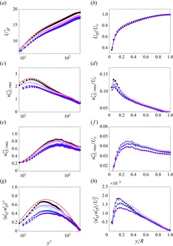


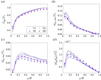


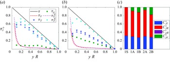


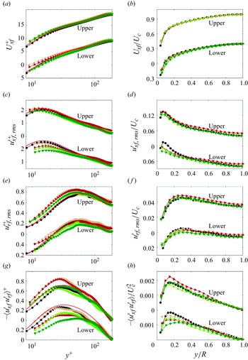


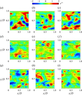


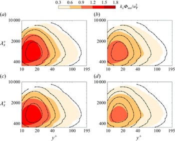


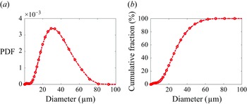


 Open access