

1. Introduction
Tip vortex cavitation is among the first forms of cavitation to appear on ship propellers and is an important design consideration for ships that require low noise and vibration levels. The vortex strength and thus the cavity thickness can be reduced by unloading the blade tip at the cost of reduced propeller efficiency. Vortex cavitation may cause broadband hull-pressure fluctuations that can lead to onboard noise and vibrations.
The broadband character can be explained by the variability of the hull pressure fluctuations between blade passages. The centre frequency of the broadband hump is expected to be due to a tip vortex cavity resonance (Ræstad Reference Ræstad1996; Bosschers Reference Bosschers2007), but this resonance behaviour is not understood. An example of a wing with a tip vortex cavity is shown in figure 6. As early as 1880, a theoretical dispersion relation was derived by Thomson (Reference Thomson1880) that describes the dynamics of waves travelling on an isolated tip vortex cavity. This was extended to include the effects of compressibility and surface tension by Morozov (Reference Morozov1974). A modification to the theory was proposed by Bosschers (Reference Bosschers2008, Reference Bosschers2009) to account for a free stream axial velocity and viscous effects. As the model for waves on a vortex cavity is neutrally stable there is no obvious criterion at which resonance can be expected.
Experiments involving sound measurements of cavitating tip vortices of wings have shown distinct tonal frequencies (Higuchi, Arndt & Rogers Reference Higuchi, Arndt and Rogers1989; Astolfi et al. Reference Astolfi, Billard, Dorange and Fruman1998). Briançon-Marjollet & Merle (Reference Briançon-Marjollet and Merle1997) measured the velocity distribution, the cavity diameter and sound of a tip vortex cavity trailing from a wing. A correlation of the sound measurements was made to the frequency of the centreline displacement mode and the elliptic deformation mode in the limit of small wavenumbers as given by Morozov (Reference Morozov1974). However, as no high-speed video recordings were available the sound could not directly be related to vortex cavity deformations.
The most detailed study to date is by Maines & Arndt (Reference Maines and Arndt1997) who used high-speed video recordings to investigate the relation between deformations of a tip vortex cavity and a distinct frequency component in the measured sound. The resonance frequencies obtained from sound measurements were related to a criterion with zero phase velocity but the high-speed video data for this study was also not sufficient to validate the analytic model used to explain the tip vortex cavity resonance frequency. An alternative explanation was provided by Bosschers (Reference Bosschers2009) who related the experimental data to the criterion of zero group velocity of the mode involving cavity volume variations. A group-speed criterion was used by Keller & Escudier (Reference Keller and Escudier1980) to explain the occurrence and wavelengths of standing waves on a cavitating vortex in a vortex tube.
This shows that there is a disagreement in the deformation mode which is thought to be responsible for the vortex cavity resonance. The underlying theoretical dispersion relation which is used to describe this criterion varies slightly between authors but has never been validated. The main goal of the present paper is to provide an understanding of the dynamics of waves on a tip vortex cavity by computing a frequency–wavenumber diagram for different cavity deformation modes using detailed high-speed video recordings. In this diagram, distinct features can be distinguished with varying phase velocity and group velocity. Most of these features can be related to the theoretical dispersion relation.
The high-speed video observations are made of a tip vortex cavity generated by a stationary wing of elliptical planform in the Delft cavitation tunnel. To also be able to study the criterion of cavity resonance, tests are performed on a wing similar in geometry to the one used by Maines & Arndt (Reference Maines and Arndt1997).
In the next section the analytical model for vortex cavity deformations is described. Then, the details of the experimental set-up are given. The results are discussed to gain an understanding of the dynamics of the vortex cavity. Based on the results the validity of the analytical model is assessed and used to define the criterion for a cavity resonance frequency. Finally, the differences in findings compared to the previous studies (Higuchi et al. Reference Higuchi, Arndt and Rogers1989; Maines & Arndt Reference Maines and Arndt1997; Astolfi et al. Reference Astolfi, Billard, Dorange and Fruman1998) are discussed.
2. Theoretical dispersion relation
The starting point for the derivation of the dispersion relation is the convected Helmholtz equation for a disturbance velocity potential $\tilde{{\it\varphi}}$
(Howe Reference Howe2003):
$\tilde{{\it\varphi}}$
(Howe Reference Howe2003):
 $$\begin{eqnarray}{\rm\nabla}^{2}\tilde{{\it\varphi}}-\frac{1}{c^{2}}\left(\frac{\partial }{\partial t}+\boldsymbol{U}\boldsymbol{\cdot }\boldsymbol{{\rm\nabla}}\right)^{2}\tilde{{\it\varphi}}=0,\end{eqnarray}$$
in which $c$
corresponds to the speed of sound and
$c$
corresponds to the speed of sound and $\boldsymbol{U}$
to the free stream velocity vector. The free stream flow needs to be irrotational with a velocity magnitude much smaller than the speed of sound. A cylindrical coordinate system
$\boldsymbol{U}$
to the free stream velocity vector. The free stream flow needs to be irrotational with a velocity magnitude much smaller than the speed of sound. A cylindrical coordinate system $(r,{\it\theta},x)$
will be adopted with a harmonic variation of the disturbance potential given by:
$(r,{\it\theta},x)$
will be adopted with a harmonic variation of the disturbance potential given by:
 $$\begin{eqnarray}\tilde{{\it\varphi}}={\it\phi}(r)\text{e}^{\text{i}(k_{x}x+n{\it\theta}-{\it\omega}t)},\end{eqnarray}$$
in which ${\it\phi}(r)$
corresponds to a potential that is only a function of radius,
${\it\phi}(r)$
corresponds to a potential that is only a function of radius, $k_{x}$
corresponds to the axial wavenumber,
$k_{x}$
corresponds to the axial wavenumber, $n$
is the azimuthal wavenumber (which must be an integer) and
$n$
is the azimuthal wavenumber (which must be an integer) and ${\it\omega}$
the angular frequency. Using only the axial free stream velocity component
${\it\omega}$
the angular frequency. Using only the axial free stream velocity component $W$
in
$W$
in $\boldsymbol{U}$
leads to the equation
$\boldsymbol{U}$
leads to the equation
 $$\begin{eqnarray}{\it\phi}^{\prime \prime }+\frac{{\it\phi}^{\prime }}{r}+\left[-k_{x}^{2}-\frac{n^{2}}{r^{2}}+\frac{1}{c^{2}}({\it\omega}-Wk_{x})^{2}\right]{\it\phi}=0,\end{eqnarray}$$
where a prime denotes a derivative with respect to the radius. When introducing the projected acoustic wavenumber in the radial direction $k_{r}$
defined as
$k_{r}$
defined as
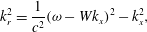 $$\begin{eqnarray}k_{r}^{2}=\frac{1}{c^{2}}({\it\omega}-Wk_{x})^{2}-k_{x}^{2},\end{eqnarray}$$
and considering that the vortex is radiating sound away from the core of the vortex, the solution for the disturbance potential is given by a Hankel function of the first kind:
 $$\begin{eqnarray}\tilde{{\it\varphi}}=\hat{{\it\phi}}\,H_{n}^{1}(k_{r}r)\text{e}^{\text{i}(k_{x}x+n{\it\theta}-{\it\omega}t)},\end{eqnarray}$$
in which $\hat{{\it\phi}}$
is the amplitude of the disturbance potential.
$\hat{{\it\phi}}$
is the amplitude of the disturbance potential.
The velocity components in $\boldsymbol{U}$
should include both the axial free stream velocity and the azimuthal velocity due to the vortex, but the addition of an azimuthal velocity leads to a Matthieu equation for which no analytical solution is available. For low frequencies and the typical vortex strengths used here, the additional terms are small for modes
$\boldsymbol{U}$
should include both the axial free stream velocity and the azimuthal velocity due to the vortex, but the addition of an azimuthal velocity leads to a Matthieu equation for which no analytical solution is available. For low frequencies and the typical vortex strengths used here, the additional terms are small for modes $n=1$
and
$n=1$
and $n=2$
as the velocity is divided by the speed of sound and are here neglected. For the mode
$n=2$
as the velocity is divided by the speed of sound and are here neglected. For the mode $n=0$
no additional terms arise. The introduction of the azimuthal velocity then gives an identical equation to (2.3).
$n=0$
no additional terms arise. The introduction of the azimuthal velocity then gives an identical equation to (2.3).
The distortion of the cavitating vortex with average radius $r_{c}$
is described by a number of modes characterised by
$r_{c}$
is described by a number of modes characterised by $k_{x}$
,
$k_{x}$
, $n$
,
$n$
, ${\it\omega}$
and amplitude
${\it\omega}$
and amplitude $\hat{r}$
. For small amplitudes, the local cavity radius
$\hat{r}$
. For small amplitudes, the local cavity radius ${\it\eta}$
is given by
${\it\eta}$
is given by
 $$\begin{eqnarray}{\it\eta}=r_{c}+\tilde{r}=r_{c}+\hat{r}\text{e}^{\text{i}(k_{x}x+n{\it\theta}-{\it\omega}t)}.\end{eqnarray}$$
The mode $n=0$
corresponds to a breathing mode and involves volume variations. Mode
$n=0$
corresponds to a breathing mode and involves volume variations. Mode $n=1$
corresponds to a serpentine mode, also called bending mode, helical mode or displacement mode, as it is the only mode that leads to a displacement of the vortex centreline. The mode
$n=1$
corresponds to a serpentine mode, also called bending mode, helical mode or displacement mode, as it is the only mode that leads to a displacement of the vortex centreline. The mode $n=2$
is the bell mode or double helix or fluted mode, and leads to an elliptical shape of the vortex core. A visualisation of the modes is presented in figure 1. The distortions are transversely propagating inertial waves and are often referred to as Kelvin waves (Saffman Reference Saffman1995).
$n=2$
is the bell mode or double helix or fluted mode, and leads to an elliptical shape of the vortex core. A visualisation of the modes is presented in figure 1. The distortions are transversely propagating inertial waves and are often referred to as Kelvin waves (Saffman Reference Saffman1995).
Main vortex cavity oscillation modes reproduced from Bosschers (Reference Bosschers2008). With (a) monopole breathing $n=0$
mode, (b) dipole serpentine
$n=0$
mode, (b) dipole serpentine $n=1$
centreline displacement mode and (c) quadrupole helical
$n=1$
centreline displacement mode and (c) quadrupole helical $n=2$
mode.
$n=2$
mode.

The equations to find the dispersion relation are obtained by using a small perturbation analysis for the kinematic and dynamic boundary conditions. The small perturbation in cavity radius with amplitude $\tilde{r}$
will result in a perturbation velocity given by the spatial derivative of the potential
$\tilde{r}$
will result in a perturbation velocity given by the spatial derivative of the potential $\tilde{{\it\varphi}}$
. The derivations by Thomson (Reference Thomson1880) and Morozov (Reference Morozov1974) use a formulation for the azimuthal velocity
$\tilde{{\it\varphi}}$
. The derivations by Thomson (Reference Thomson1880) and Morozov (Reference Morozov1974) use a formulation for the azimuthal velocity $V$
valid for potential flow, but we show here that, at least for
$V$
valid for potential flow, but we show here that, at least for $n=0$
, the dispersion relation can also be derived for a viscous vortex formulation. In both formulations a zero mean radial velocity
$n=0$
, the dispersion relation can also be derived for a viscous vortex formulation. In both formulations a zero mean radial velocity $U$
and a constant mean axial velocity component
$U$
and a constant mean axial velocity component $W$
are used. The mean velocities for potential flow in which a vortex with circulation
$W$
are used. The mean velocities for potential flow in which a vortex with circulation ${\it\Gamma}$
is present are then given by
${\it\Gamma}$
is present are then given by
 $$\begin{eqnarray}\boldsymbol{U}=(U,V,W)=\left(0,\,\frac{{\it\Gamma}}{2{\rm\pi}r},\,W\right).\end{eqnarray}$$
For viscous flow, the situation is more complicated. Neglecting the flow inside the cavity, the azimuthal velocity in a viscous fluid has to satisfy a zero shear stress boundary condition at the cavity interface, which leads to a different behaviour of the velocity near the cavity interface when compared to the non-cavitating vortex as shown in Bosschers (Reference Bosschers2015). However, this change in velocity leads to a small change in pressure at the cavity radius from which it is concluded that a formulation for the azimuthal velocity of a non-cavitating vortex can also be used to find the relation between cavity size and pressure. We will use here the Burnham–Hallock model (Burnham & Hallock Reference Burnham and Hallock1982) due its simple formulation for the pressure variation. The azimuthal velocity at radius $r$
for a vortex with viscous core radius
$r$
for a vortex with viscous core radius $r_{v}$
is given by
$r_{v}$
is given by
 $$\begin{eqnarray}V=\frac{{\it\Gamma}}{2{\rm\pi}}\frac{r}{r_{v}^{2}+r^{2}}.\end{eqnarray}$$
The kinematic boundary condition for $f=r-{\it\eta}$
is given by
$f=r-{\it\eta}$
is given by
 $$\begin{eqnarray}\frac{\text{D}f}{\text{D}t}=\frac{\partial f}{\partial t}+(\boldsymbol{U}+\boldsymbol{{\rm\nabla}}\tilde{{\it\varphi}})\boldsymbol{\cdot }\boldsymbol{{\rm\nabla}}f=0.\end{eqnarray}$$
Only the linear terms of the perturbations in potential and cavity radius will be retained, which implies that the equation contains only the perturbation velocity in the radial direction and the derivative of the ${\it\eta}$
perturbation in time, axial direction and azimuthal direction:
${\it\eta}$
perturbation in time, axial direction and azimuthal direction:
 $$\begin{eqnarray}\hat{{\it\phi}}\,k_{r}H_{n}^{1^{\prime }}(k_{r}r_{c})-\left(-\text{i}{\it\omega}+W\text{i}k_{x}+V_{c}\frac{\text{i}n}{r_{c}}\right)\hat{r}=0,\end{eqnarray}$$
where the prime again denotes the derivative to $r$
and
$r$
and $V_{c}$
is the mean azimuthal velocity at the cavity interface
$V_{c}$
is the mean azimuthal velocity at the cavity interface $r=r_{c}$
.
$r=r_{c}$
.
The dynamic boundary condition states that the pressure at the cavity interface has to be equal to the vapour pressure. For potential flow, the Bernoulli equation can be used as done in Thomson (Reference Thomson1880) and Morozov (Reference Morozov1974). Here, we will start from the radial momentum equation to investigate if a viscous vortex solution can be applied. The radial momentum equation is given by
 $$\begin{eqnarray}-\frac{1}{{\it\rho}}\frac{\partial p}{\partial r}=\frac{\partial }{\partial t}\frac{\partial \tilde{{\it\varphi}}}{\partial r}+(\boldsymbol{U}+\boldsymbol{{\rm\nabla}}\tilde{{\it\varphi}})\boldsymbol{\cdot }\boldsymbol{{\rm\nabla}}\frac{\partial \tilde{{\it\varphi}}}{\partial r}-\frac{\displaystyle \left(V+\frac{\partial \tilde{{\it\varphi}}}{r\partial {\it\theta}}\right)^{2}}{r}.\end{eqnarray}$$
If we take only the linear terms into account, the equation reads:
 $$\begin{eqnarray}-\frac{1}{{\it\rho}}\frac{\partial p}{\partial r}=\frac{\partial }{\partial t}\frac{\partial \tilde{{\it\varphi}}}{\partial r}+W\frac{\partial }{\partial x}\frac{\partial \tilde{{\it\varphi}}}{\partial r}+V\frac{\partial }{r\partial {\it\theta}}\frac{\partial \tilde{{\it\varphi}}}{\partial r}-\frac{V^{2}}{r}-\frac{2V}{r}\frac{\partial \tilde{{\it\varphi}}}{r\partial {\it\theta}}.\end{eqnarray}$$
The first two terms on the right-hand side can be directly integrated. The third and fifth terms on the right-hand side can only be integrated if a potential flow solution is assumed for $V$
, but these terms vanish for the mode
$V$
, but these terms vanish for the mode $n=0$
as the azimuthal disturbance velocity equals zero for this mode. The fourth term can be integrated using either (2.7) or (2.8) for the azimuthal velocity. The integration for this fourth term using (2.8) gives for the pressure in the liquid at the cavity interface
$n=0$
as the azimuthal disturbance velocity equals zero for this mode. The fourth term can be integrated using either (2.7) or (2.8) for the azimuthal velocity. The integration for this fourth term using (2.8) gives for the pressure in the liquid at the cavity interface $r={\it\eta}$
:
$r={\it\eta}$
:
 $$\begin{eqnarray}p_{v}-p_{T}+\frac{1}{2}{\it\rho}\left(\frac{{\it\Gamma}}{2{\rm\pi}}\right)^{2}\frac{1}{(r_{v}^{2}+{\it\eta}^{2})}=p_{\infty },\end{eqnarray}$$
where $p_{v}$
corresponds to the vapour pressure,
$p_{v}$
corresponds to the vapour pressure, $p_{T}$
to the contribution of surface tension and
$p_{T}$
to the contribution of surface tension and $p_{\infty }$
to the free stream pressure in absence of the vortex. Assuming a small amplitude
$p_{\infty }$
to the free stream pressure in absence of the vortex. Assuming a small amplitude $\tilde{r}$
with respect to
$\tilde{r}$
with respect to $r_{c}$
, the equation can be written as
$r_{c}$
, the equation can be written as
 $$\begin{eqnarray}p_{v}-p_{T}+\frac{1}{2}{\it\rho}\left(\frac{{\it\Gamma}}{2{\rm\pi}}\right)^{2}\frac{1}{(r_{v}^{2}+r_{c}^{2})}-{\it\rho}\left(\frac{{\it\Gamma}}{2{\rm\pi}}\right)^{2}\frac{\tilde{r}r_{c}}{(r_{v}^{2}+r_{c}^{2})^{2}}=p_{\infty }.\end{eqnarray}$$
The contribution due to surface tension $T$
at
$T$
at $r={\it\eta}$
is given by:
$r={\it\eta}$
is given by:
 $$\begin{eqnarray}\displaystyle p_{T} & = & \displaystyle T\left(\frac{\partial ^{2}}{\partial x^{2}}+\frac{\partial ^{2}}{\partial r^{2}}+\frac{1}{r}\frac{\partial }{\partial r}+\frac{1}{r^{2}}\frac{\partial ^{2}}{\partial {\it\theta}^{2}}\right)(r-[r_{c}+\tilde{r}])\nonumber\\ \displaystyle & = & \displaystyle T\left(k_{x}^{2}+\frac{1}{{\it\eta}^{2}}n^{2}\right)\tilde{r}+T\frac{1}{{\it\eta}}\nonumber\\ \displaystyle & = & \displaystyle \frac{T}{r_{c}}\left[1+(n^{2}+k_{x}^{2}r_{c}^{2}-1)\frac{\tilde{r}}{r_{c}}\right],\end{eqnarray}$$
where again a linearisation has been applied for the perturbation of the cavity radius. For the situation with zero perturbation, the difference in pressure between the free stream and at the mean cavity radius due to the mean azimuthal velocity is
 $$\begin{eqnarray}p_{\infty }-p_{c}=\frac{1}{2}{\it\rho}\left(\frac{{\it\Gamma}}{2{\rm\pi}}\right)^{2}\frac{1}{(r_{v}^{2}+r_{c}^{2})},\end{eqnarray}$$
with the pressure at the cavity interface given by
 $$\begin{eqnarray}p_{v}-\frac{T}{r_{c}}-p_{c}=0.\end{eqnarray}$$
The contribution of the term containing $\tilde{r}$
in (2.14), referred to as
$\tilde{r}$
in (2.14), referred to as $\tilde{p}_{c,4}$
, with subscript 4 referring to the fourth term in (2.14), can be written as:
$\tilde{p}_{c,4}$
, with subscript 4 referring to the fourth term in (2.14), can be written as:
 $$\begin{eqnarray}\tilde{p}_{c,4}={\it\rho}\left(\frac{{\it\Gamma}}{2{\rm\pi}}\right)^{2}\frac{\tilde{r}r_{c}}{(r_{v}^{2}+r_{c}^{2})^{2}}={\it\rho}V_{c}^{2}\frac{\tilde{r}}{r_{c}}.\end{eqnarray}$$
This relation between $\tilde{p}_{c,4}$
and
$\tilde{p}_{c,4}$
and $V_{c}$
derived for the Burnham–Hallock vortex model is identical to that for a vortex in potential flow given by (2.7), and it will be assumed in the following that this relation is generally valid and can also be used for viscous vortex formulations different from the Burnham–Hallock model.
$V_{c}$
derived for the Burnham–Hallock vortex model is identical to that for a vortex in potential flow given by (2.7), and it will be assumed in the following that this relation is generally valid and can also be used for viscous vortex formulations different from the Burnham–Hallock model.
The sum of all terms in (2.12) containing perturbations to the pressure should be equal to zero, which gives
 $$\begin{eqnarray}\frac{T}{r_{c}}(n^{2}+k_{x}^{2}r_{c}^{2}-1)\frac{\tilde{r}}{r_{c}}-{\it\rho}V_{c}^{2}\frac{\tilde{r}}{r_{c}}+\text{i}{\it\rho}\left(k_{x}W+\frac{V_{c}n}{r_{c}}-{\it\omega}\right)\tilde{{\it\varphi}}=0.\end{eqnarray}$$
Combining the kinematic boundary condition (2.10) and the dynamic boundary condition (2.19) leads to the dispersion relation:
 $$\begin{eqnarray}{\it\omega}_{1,2}=Wk_{x}+{\it\Omega}\left[n\pm \sqrt{\frac{-k_{r}r_{c}H_{n}^{1^{\prime }}(k_{r}r_{c})}{H_{n}^{1}(k_{r}r_{c})}\;T_{{\it\omega}}}\right],\end{eqnarray}$$
in which ${\it\Omega}=V_{c}/r_{c}$
and
${\it\Omega}=V_{c}/r_{c}$
and $T_{{\it\omega}}$
includes the contribution of the surface tension:
$T_{{\it\omega}}$
includes the contribution of the surface tension:
 $$\begin{eqnarray}T_{{\it\omega}}=\sqrt{1+\frac{T}{{\it\rho}r_{c}V_{c}^{2}}(n^{2}+k_{x}^{2}r_{c}^{2}-1)}.\end{eqnarray}$$
Each vibration mode contains two frequencies corresponding to the plus and minus sign on the right-hand side of (2.20). This sign is also used in the following for the identification of the mode. The contribution of the surface tension will not be discussed further as its influence is very small for the case considered. As both frequencies are real numbers the perturbations are neutrally stable. If the axial velocity $W$
is small with respect to the speed of sound, the criterion for a sound wave to occur is that the radial wavenumber squared, defined by (2.4), is larger than zero. This results in the condition
$W$
is small with respect to the speed of sound, the criterion for a sound wave to occur is that the radial wavenumber squared, defined by (2.4), is larger than zero. This results in the condition
 $$\begin{eqnarray}\left|\frac{c_{p,x}}{c}\right|=\left|\frac{k}{k_{x}}\right|>1,\end{eqnarray}$$
where $c_{p,x}={\it\omega}/k_{x}$
corresponds to the axial phase velocity and
$c_{p,x}={\it\omega}/k_{x}$
corresponds to the axial phase velocity and $k$
corresponds to the acoustic wavenumber in the fluid,
$k$
corresponds to the acoustic wavenumber in the fluid, $k={\it\omega}/c$
.
$k={\it\omega}/c$
.
For small axial phase velocities or low frequencies the radial wavenumber becomes imaginary and the Hankel function reduces to a modified Bessel function of the second kind $\text{K}$
. The wave in the radial direction now becomes an evanescent wave as
$\text{K}$
. The wave in the radial direction now becomes an evanescent wave as $k_{r}^{2}\cong -k_{x}^{2}$
. The dispersion relation for low frequencies is then given by
$k_{r}^{2}\cong -k_{x}^{2}$
. The dispersion relation for low frequencies is then given by
 $$\begin{eqnarray}{\it\omega}_{1,2}=Wk_{x}+{\it\Omega}\left[n\pm \sqrt{\frac{-k_{x}r_{c}{\text{K}_{n}^{1}}^{\prime }(k_{x}r_{c})}{\text{K}_{n}^{1}(k_{x}r_{c})}}\right],\end{eqnarray}$$
with the non-dimensional form given by
 $$\begin{eqnarray}\bar{{\it\omega}}_{1,2}=\frac{{\it\omega}_{1,2}r_{c}}{W}={\it\kappa}+\frac{V_{c}}{W}\left[n\pm \sqrt{\frac{-{\it\kappa}{\text{K}_{n}}^{\prime }({\it\kappa})}{\text{K}_{n}({\it\kappa})}}\right],\end{eqnarray}$$
in which a non-dimensional wavenumber ${\it\kappa}=k_{x}r_{c}\cong \text{i}\,k_{r}r_{c}$
has been introduced. For low frequencies and small axial velocities, the value of the radial wavenumber becomes approximately equal to the axial wavenumber. An example of the dispersion relation of (2.20) is given in figure 2.
${\it\kappa}=k_{x}r_{c}\cong \text{i}\,k_{r}r_{c}$
has been introduced. For low frequencies and small axial velocities, the value of the radial wavenumber becomes approximately equal to the axial wavenumber. An example of the dispersion relation of (2.20) is given in figure 2.
Dispersion relation for the two $\pm$
branches of the three modes described by (2.20). Condition;
$\pm$
branches of the three modes described by (2.20). Condition; ${\it\Omega}=2.0\times 10^{3}~\text{rad}~\text{s}^{-1}$
,
${\it\Omega}=2.0\times 10^{3}~\text{rad}~\text{s}^{-1}$
, $W=6.3~\text{m}~\text{s}^{-1}$
and
$W=6.3~\text{m}~\text{s}^{-1}$
and $r_{c}=2.3~\text{mm}$
.
$r_{c}=2.3~\text{mm}$
.

In the present formulation only outgoing waves are considered while reflections from, for instance, the wall of the test-section of the cavitation tunnel may also be present. The potential at the tunnel walls can be computed from (2.5) while assuming an evanescent wave. A typical value of the smallest relevant wavenumber on the tip vortex cavity from figure 2 and as found in the experiment is $k_{x}=\text{i}k_{r}=0.04~\text{rad}~\text{mm}^{-1}$
. The walls of the tunnel used for the experiment are at a distance
$k_{x}=\text{i}k_{r}=0.04~\text{rad}~\text{mm}^{-1}$
. The walls of the tunnel used for the experiment are at a distance $r=0.15~\text{m}$
from the tip vortex cavity. This results in a value of
$r=0.15~\text{m}$
from the tip vortex cavity. This results in a value of $k_{r}r=6$
which shows that the influence of the tunnel walls on the dispersion relation can be neglected.
$k_{r}r=6$
which shows that the influence of the tunnel walls on the dispersion relation can be neglected.
The azimuthal velocity at the cavity interface can be derived from the pressure difference. Neglecting surface tension, the formulation for the potential flow vortex gives:
 $$\begin{eqnarray}\frac{V_{c}}{W}=\sqrt{\frac{p_{\infty }-p_{v}}{\displaystyle {\textstyle \frac{1}{2}}{\it\rho}W^{2}}}=\sqrt{{\it\sigma}}.\end{eqnarray}$$
For a viscous flow vortex, the analytical formulation for the azimuthal velocity distribution of a 2-D cavitating vortex is given in Bosschers (Reference Bosschers2015). The formulation can be interpreted as a cavitating Lamb–Oseen vortex and reads:
 $$\begin{eqnarray}V=\frac{{\it\Gamma}}{2{\rm\pi}r}\left\{1-{\it\beta}\exp \left[-{\it\zeta}\frac{(r^{2}-r_{c}^{2})}{r_{v}^{2}}\right]\right\},\end{eqnarray}$$
with ${\it\beta}$
defined by
${\it\beta}$
defined by
 $$\begin{eqnarray}{\it\beta}=\frac{r_{v}^{2}}{r_{v}^{2}+{\it\zeta}r_{c}^{2}},\end{eqnarray}$$
and where ${\it\zeta}$
is a constant
${\it\zeta}$
is a constant $({\it\zeta}=1.2564)$
defined such that the maximum azimuthal velocity for a non-cavitating vortex occurs on the radius of the viscous core of the non-cavitating vortex,
$({\it\zeta}=1.2564)$
defined such that the maximum azimuthal velocity for a non-cavitating vortex occurs on the radius of the viscous core of the non-cavitating vortex, $r_{v}$
.
$r_{v}$
.
The formulation has been derived using the appropriate jump relations for the stresses at the cavity interface which gives a shear stress in the liquid at the cavity interface that is approximately zero. The condition of zero shear stress results in a small region of solid-body rotation near the cavity. The present formulation is different from the Gaussian vortex formulations proposed by Choi & Ceccio (Reference Choi and Ceccio2007) and Choi et al. (Reference Choi, Hsiao, Chahine and Ceccio2009) who introduce an additional parameter that describes the azimuthal velocity at the cavity interface. The formulation for the azimuthal velocity of the cavitating vortex still needs to be validated by detailed flow field measurements.
The equation can be used to derive an analytical expression for the pressure, which is a function of the same parameters. This formulation for the pressure at the cavity radius replaces (2.25) and reads
 $$\begin{eqnarray}{\it\sigma}=\frac{p_{\infty }-p_{v}}{\frac{1}{2}{\it\rho}W^{2}}=\frac{{\it\Gamma}^{2}}{2({\rm\pi}Wr_{c})^{2}}\left\{\begin{array}{@{}c@{}}\displaystyle \frac{1}{2}-{\it\beta}\text{e}^{-{\it\zeta}r_{c}^{2}/r_{v}^{2}}+\frac{{\it\beta}^{2}}{2}\text{e}^{-2{\it\zeta}r_{c}^{2}/r_{v}^{2}}\\ \displaystyle +\,\frac{{\it\beta}{\it\zeta}r_{c}^{2}}{r_{v}^{2}}E_{1}({\it\zeta}r_{c}^{2}/r_{v}^{2})\\ \displaystyle -\frac{{\it\beta}^{2}{\it\zeta}r_{c}^{2}}{r_{v}^{2}}E_{1}(2{\it\zeta}r_{c}^{2}/r_{v}^{2})\end{array}\right\}.\end{eqnarray}$$
with $E_{1}$
the exponential integral. The azimuthal velocity at the cavity radius now corresponds to
$E_{1}$
the exponential integral. The azimuthal velocity at the cavity radius now corresponds to
 $$\begin{eqnarray}V_{c}=\frac{{\it\Gamma}}{2{\rm\pi}r_{c}}\left\{\frac{{\it\zeta}r_{c}^{2}}{r_{v}^{2}+{\it\zeta}r_{c}^{2}}\right\}.\end{eqnarray}$$
This azimuthal velocity can be used in (2.20) and (2.23). It is recognised that the disturbance in the flow due to the cavity deformations is given by a potential flow solution, which is not consistent with the use of a viscous mean flow solution for the kinematic and dynamic boundary conditions. However, as discussed before, the contribution of the azimuthal velocity component to the free stream velocity $\boldsymbol{U}$
is expected to lead to small changes to the disturbance potential, which suggests that the use of a viscous vortex solution instead of a potential flow vortex solution will also lead to small changes to the disturbance potential. The use of a viscous flow solution for
$\boldsymbol{U}$
is expected to lead to small changes to the disturbance potential, which suggests that the use of a viscous vortex solution instead of a potential flow vortex solution will also lead to small changes to the disturbance potential. The use of a viscous flow solution for $V_{c}$
in the kinematic and dynamic boundary condition leading to (2.20) and (2.23) is only allowed for
$V_{c}$
in the kinematic and dynamic boundary condition leading to (2.20) and (2.23) is only allowed for $n=0$
and when the Burnham–Hallock vortex is used. Nevertheless, we here assume that a generic viscous flow solution can be used for all values of
$n=0$
and when the Burnham–Hallock vortex is used. Nevertheless, we here assume that a generic viscous flow solution can be used for all values of $n$
.
$n$
.
The azimuthal velocity of a non-cavitating and cavitating vortex is given in figure 3. The potential flow formulation corresponds to (2.7) and the viscous flow formulation corresponds to (2.26). The velocities are obtained using a single value of ${\it\Gamma}$
and
${\it\Gamma}$
and $r_{v}$
.
$r_{v}$
.
Velocity distribution of a potential flow vortex, Lamb–Oseen vortex and three cavitating Lamb–Oseen vortices for ${\it\Gamma}=0.1~\text{m}^{2}~\text{s}^{-1}$
and
${\it\Gamma}=0.1~\text{m}^{2}~\text{s}^{-1}$
and $r_{v}=2~\text{mm}$
.
$r_{v}=2~\text{mm}$
.

3. Experimental set-up
The experimental facility is the cavitation tunnel in the Laboratory for Ship Hydrodynamics at Delft University of Technology. A detailed description of the tunnel is given by Foeth (Reference Foeth2008), while the recent modifications are described by Zverkhovskyi (Reference Zverkhovskyi2014).
The maximum free stream tunnel velocity $U_{\infty }$
is
$U_{\infty }$
is $7~\text{m}~\text{s}^{-1}$
, which is approximately the velocity used in the results presented here. The cross section is
$7~\text{m}~\text{s}^{-1}$
, which is approximately the velocity used in the results presented here. The cross section is $0.30\times 0.30~\text{m}^{2}$
at the inlet, but changes downstream in vertical direction to
$0.30\times 0.30~\text{m}^{2}$
at the inlet, but changes downstream in vertical direction to $0.30\times 0.32~\text{m}^{2}$
at the outlet to compensate for boundary layer growth, so that there is no streamwise pressure gradient in the test section. A sketch of the set-up is given in figure 4. The coordinate system with the wing tip at the origin is defined with
$0.30\times 0.32~\text{m}^{2}$
at the outlet to compensate for boundary layer growth, so that there is no streamwise pressure gradient in the test section. A sketch of the set-up is given in figure 4. The coordinate system with the wing tip at the origin is defined with $x$
pointing in the streamwise direction. The top plane (
$x$
pointing in the streamwise direction. The top plane ( $xz$
) includes the elliptic wing planform with
$xz$
) includes the elliptic wing planform with $z$
in the spanwise direction, positive from root to tip. Illumination in the side plane (
$z$
in the spanwise direction, positive from root to tip. Illumination in the side plane ( $xy$
) is partly blocked by the wing mount in the tunnel. The lift direction
$xy$
) is partly blocked by the wing mount in the tunnel. The lift direction $y$
is vertically downward.
$y$
is vertically downward.
Experimental configuration (not to scale) in the cavitation tunnel with tip vortex cavity A, hydrophone B, disk C holding elliptic planform wing D and high-speed cameras E: (a) top view, (b) side view.

Tip vortex cavitation is generated by a half-model wing of elliptic planform with an aspect ratio of 3 and a $\mathit{NACA}~66_{2}{-}415$
cross section with
$\mathit{NACA}~66_{2}{-}415$
cross section with $a=0.8$
mean line. The trailing edge was truncated at a thickness of 0.3 mm due to manufacturing limitations. The chord length after truncation is 0.1256 m. The wing has a half span of 0.150 m, so that the tip is positioned in the centre of the test section. The wing is mounted with the spanwise direction horizontally, with the suction side pointed downward, on the side window of the test section on a disk containing a six-component force/torque sensor (ATI SI-330-30).
$a=0.8$
mean line. The trailing edge was truncated at a thickness of 0.3 mm due to manufacturing limitations. The chord length after truncation is 0.1256 m. The wing has a half span of 0.150 m, so that the tip is positioned in the centre of the test section. The wing is mounted with the spanwise direction horizontally, with the suction side pointed downward, on the side window of the test section on a disk containing a six-component force/torque sensor (ATI SI-330-30).
The water temperature is measured with a PT-100 sensor placed in a quiescent corner outside the main flow downstream of the test section. A digital pressure transmitter (Keller PAA 33X) mounted in the throat of the contraction upstream of the test section gives the absolute pressure near the wing at a data acquisition rate of 10 Hz. The free stream tunnel velocity is determined from the pressure drop over the contraction measured with a differential pressure sensor (Validyne DP 15) with a number 36 membrane. Both the values of the absolute pressure sensor and the velocity based on the pressure drop are corrected with a reference measurement using a pitot tube, in an empty test section at the location of the wing.
The dissolved oxygen concentration (DO) was used as a measure of the amount of dissolved gas in the water. A fluorescence-based optical sensor (RDO Pro) was placed in a sample of water taken from the tunnel at the start and end of each day. The typical accuracy of the sensor is $0.1~\text{mg}~\text{l}^{-1}$
, but due to fluctuations in concentration in the tunnel,
$0.1~\text{mg}~\text{l}^{-1}$
, but due to fluctuations in concentration in the tunnel, $0.5~\text{mg}~\text{l}^{-1}$
is the smallest practical division. As only dissolved oxygen is measured this is taken as a representative indicator for the total amount of dissolved gas.
$0.5~\text{mg}~\text{l}^{-1}$
is the smallest practical division. As only dissolved oxygen is measured this is taken as a representative indicator for the total amount of dissolved gas.
A hydrophone (Brüel & Kjær type 8103) and a measurement amplifier (Brüel & Kjær type 2606) were used to measure the radiated sound. The hydrophone was inside a water-filled cup mounted on the window opposite the wing at the vertical position of the tip and the streamwise position of the trailing edge. All sensors were sampled at a rate of 40 kHz which is well above the 1.5 kHz upper limit of the relevant frequency range.
Two high-speed cameras (LaVision Imager Pro HS) in combination with two backlight LED panels gave a shadowgraphy image of the tip vortex cavity at $5\times 10^{3}$
f.p.s. The total recording time, limited by the camera memory, was six seconds. The top view
$5\times 10^{3}$
f.p.s. The total recording time, limited by the camera memory, was six seconds. The top view $xz$
-plane camera is equipped with a Nikon AF Nikkor 35 mm objective at a
$xz$
-plane camera is equipped with a Nikon AF Nikkor 35 mm objective at a $f$
-stop value of 2 with an approximate object focal-plane distance of 0.50 m. The disk holding the wing blocks part of the field of view of the side view
$f$
-stop value of 2 with an approximate object focal-plane distance of 0.50 m. The disk holding the wing blocks part of the field of view of the side view $xy$
-plane camera. Consequently a 55 mm Micro-Nikkor set to
$xy$
-plane camera. Consequently a 55 mm Micro-Nikkor set to $f$
-stop of 2.8 is used at a object focal-plane distance of 0.57 m.
$f$
-stop of 2.8 is used at a object focal-plane distance of 0.57 m.
Edge detection of the tip vortex cavity is based on gradients in light intensity in the image. A Canny (Reference Canny1986) edge detection method was used with a relative gray value intensity threshold of 0.1 and a filter size of 1.0. Units and detailed description of these parameters can be found in Canny (Reference Canny1986). In the $xz$
-plane the tip of the wing is in the field of view and is used to define the origin. As contrast is needed to detect the cavity edge the detected range is between
$xz$
-plane the tip of the wing is in the field of view and is used to define the origin. As contrast is needed to detect the cavity edge the detected range is between $x/c_{0}=0.19$
to
$x/c_{0}=0.19$
to $x/c_{0}=2.48$
downstream of the tip resulting in an equivalent pixel size of 0.16 mm in the object domain. The edge of the disk holding the wing in the
$x/c_{0}=2.48$
downstream of the tip resulting in an equivalent pixel size of 0.16 mm in the object domain. The edge of the disk holding the wing in the $xy$
-plane is taken as
$xy$
-plane is taken as $y=0$
. The cavity extent is between
$y=0$
. The cavity extent is between $x/c_{0}=1.12$
and
$x/c_{0}=1.12$
and $x/c_{0}=2.60$
downstream of the tip with an equivalent pixel size of 0.10 mm in the object domain. The overlap area between both views where 3-D diameter and location information is available spans
$x/c_{0}=2.60$
downstream of the tip with an equivalent pixel size of 0.10 mm in the object domain. The overlap area between both views where 3-D diameter and location information is available spans $1.35\,c_{0}$
.
$1.35\,c_{0}$
.
The pixelization of the diameter and location data are removed by using a fourth order Chebyshev type II low-pass filter. The cut-off frequency was set to half the Nyquist frequency in both cases. The spatial Nyquist frequency is $20~\text{rad}~\text{mm}^{-1}$
in the
$20~\text{rad}~\text{mm}^{-1}$
in the $xz$
-plane and
$xz$
-plane and $32~\text{rad}~\text{mm}^{-1}$
in the
$32~\text{rad}~\text{mm}^{-1}$
in the $xy$
-plane. The low-pass filters were applied in forward and reverse direction to prevent phase shift and to double the effective filter order.
$xy$
-plane. The low-pass filters were applied in forward and reverse direction to prevent phase shift and to double the effective filter order.
4. Results
The results are presented as follows. First the sensitivity of the mean cavity diameter to dissolved gas and free stream velocity fluctuations is discussed. Second, an overview is given of diameter oscillations in the time domain combined with a description of the stationary cavity geometry. Third, a frequency–wavenumber diagram is generated to validate the analytical model for the dispersion relation. Fourth, a comparison is made between sound, wing forces and cavity oscillations. Finally, the frequency of the peak in the cavity diameter spectrum is compared to the frequency of the zero group velocity criterion that can be derived from the analytical dispersion relation and a comparison is made to the data of the ‘singing’ vortex as given in Maines & Arndt (Reference Maines and Arndt1997).
4.1. Dissolved oxygen concentration
In the dispersion relation for the vortex cavity the pressure inside the cavity is assumed to be equal to the vapour pressure. Preparations for the test conditions where a steady tip vortex cavity is present can take typically 5 min or more during which the tunnel is in operation. Therefore there is sufficient opportunity for dissolved non-condensable gas to diffuse into the cavity. Figure 5 is the result of a sensitivity study to show the importance of a low dissolved gas concentration to obtain reproducible results. For concentrations below $3.8~\text{mg}~\text{l}^{-1}$
, the results show acceptably similar values for cavitation numbers above 1.3.
$3.8~\text{mg}~\text{l}^{-1}$
, the results show acceptably similar values for cavitation numbers above 1.3.
Mean cavity diameter in the $xz$
-plane as a function of the cavitation number for a lift coefficient of
$xz$
-plane as a function of the cavitation number for a lift coefficient of $C_{L}=0.58$
and a Reynolds number based on the wing-root chord of
$C_{L}=0.58$
and a Reynolds number based on the wing-root chord of $\mathit{Re}=9\times 10^{5}$
. Data points are grouped according to dissolved oxygen concentration. The vertical error bars are the streamwise variation of the time-averaged cavity diameter, which is an indication of the size of the stationary wave amplitude as seen in figure 6. The horizontal error bars denote the variation in cavitation number. The model vortex lines represent the result of (2.25) for a potential flow vortex and (2.28) for a cavitating Lamb–Oseen vortex using
$\mathit{Re}=9\times 10^{5}$
. Data points are grouped according to dissolved oxygen concentration. The vertical error bars are the streamwise variation of the time-averaged cavity diameter, which is an indication of the size of the stationary wave amplitude as seen in figure 6. The horizontal error bars denote the variation in cavitation number. The model vortex lines represent the result of (2.25) for a potential flow vortex and (2.28) for a cavitating Lamb–Oseen vortex using ${\it\Gamma}=0.10~\text{m}^{2}~\text{s}^{-1}$
and
${\it\Gamma}=0.10~\text{m}^{2}~\text{s}^{-1}$
and $r_{v}=1.7~\text{mm}$
.
$r_{v}=1.7~\text{mm}$
.

For a cavitation number of 1.1 the standard deviation in core diameter for concentrations of $3.2{-}3.8~\text{mg}~\text{l}^{-1}$
is larger than for lower concentrations. The general increase in standard deviation is due to the change of the cavity from a cylindrical shape into a twisted ribbon-like cavity shape as shown in figure 6. At concentrations above
$3.2{-}3.8~\text{mg}~\text{l}^{-1}$
is larger than for lower concentrations. The general increase in standard deviation is due to the change of the cavity from a cylindrical shape into a twisted ribbon-like cavity shape as shown in figure 6. At concentrations above $4.0~\text{mg}~\text{l}^{-1}$
an increase in standard deviation is found for cavitation numbers below 2.2.
$4.0~\text{mg}~\text{l}^{-1}$
an increase in standard deviation is found for cavitation numbers below 2.2.
Combination of vortex cavity images in $xz$
-plane on top and
$xz$
-plane on top and $xy$
-plane on the bottom of each image. Flow is from left to right with the elliptical black object the pressure side of the wing. (a) Conditions;
$xy$
-plane on the bottom of each image. Flow is from left to right with the elliptical black object the pressure side of the wing. (a) Conditions; $C_{L}=0.58$
,
$C_{L}=0.58$
, ${\it\sigma}=0.87$
,
${\it\sigma}=0.87$
, $\mathit{Re}=9.1\times 10^{5}$
and
$\mathit{Re}=9.1\times 10^{5}$
and $\mathit{DO}=2.7~\text{mg}~\text{l}^{-1}$
. (b) Conditions;
$\mathit{DO}=2.7~\text{mg}~\text{l}^{-1}$
. (b) Conditions; $C_{L}=0.58$
,
$C_{L}=0.58$
, ${\it\sigma}=1.55$
,
${\it\sigma}=1.55$
, $\mathit{Re}=9.1\times 10^{5}$
and
$\mathit{Re}=9.1\times 10^{5}$
and $\mathit{DO}=4.4~\text{mg}~\text{l}^{-1}$
. (c) Conditions;
$\mathit{DO}=4.4~\text{mg}~\text{l}^{-1}$
. (c) Conditions; $C_{L}=0.46$
,
$C_{L}=0.46$
, ${\it\sigma}=1.07$
,
${\it\sigma}=1.07$
, $\mathit{Re}=8.9\times 10^{5}$
and
$\mathit{Re}=8.9\times 10^{5}$
and $\mathit{DO}=2.7~\text{mg}~\text{l}^{-1}$
.
$\mathit{DO}=2.7~\text{mg}~\text{l}^{-1}$
.

The results based on a potential flow vortex give an upper limit to the cavity size as this vortex provides an overestimation of the azimuthal velocity, resulting in a lower pressure and thus a larger cavity. The cavitating Lamb–Oseen model takes the viscous core into account, which reduces the azimuthal velocity and gives a smaller estimate for the diameter, which compares reasonably with the spread in the experimental data.
In the current experiment, the drive system of the cavitation tunnel was run at a constant rotation rate of 700 revolutions $\text{min}^{-1}$
. Because of an unidentified flow instability in the tunnel, there are large-scale non-periodic velocity excursions as high as 10 % of the mean. Within the six-second measurement time used, the standard deviation of the velocity in each measurement remained below 5 % with a typical value of 2.5 %. As the fluctuations are not periodic, the time for the flow to meet this condition can vary between measurements. A period with low standard deviation was selected by monitoring the tunnel velocity in real time. The consequence of this approach is a difference between measurements in the time for which the cavity is exposed to over-saturated water.
$\text{min}^{-1}$
. Because of an unidentified flow instability in the tunnel, there are large-scale non-periodic velocity excursions as high as 10 % of the mean. Within the six-second measurement time used, the standard deviation of the velocity in each measurement remained below 5 % with a typical value of 2.5 %. As the fluctuations are not periodic, the time for the flow to meet this condition can vary between measurements. A period with low standard deviation was selected by monitoring the tunnel velocity in real time. The consequence of this approach is a difference between measurements in the time for which the cavity is exposed to over-saturated water.
Long exposure times of the tip vortex cavity to over-saturated water and excursions to lower pressures due to higher free stream velocities promote diffusion of gas into the cavity. This increases the mean cavity diameter and promotes the appearance of a stationary wave for higher cavitation numbers. This is expected to be the cause for the decrease in cavity diameter between ${\it\sigma}=1.6$
and
${\it\sigma}=1.6$
and ${\it\sigma}=1.4$
for dissolved oxygen concentrations above
${\it\sigma}=1.4$
for dissolved oxygen concentrations above $4.0~\text{mg}~\text{l}^{-1}$
as seen in figure 5.
$4.0~\text{mg}~\text{l}^{-1}$
as seen in figure 5.
4.2. Cavity dynamics in time and frequency domain
For the detailed evaluation of the cavity dynamics a single condition is selected corresponding to figure 6(b). Out of seven cases with significant volume variations, this case shows the largest indication for a cavity eigenfrequency. In this case the dissolved gas in the water is highly over-saturated. For later comparison, the condition of figure 6(c) is used. This is at the minimum dissolved gas concentration possible in the cavitation tunnel.
The temporal cavity diameter oscillations are expected to be a combination of the $n=0^{\pm }$
and
$n=0^{\pm }$
and $n=2^{\pm }$
modes as presented in figure 1. As two separate views are available, the identification has to be made by combining both views. Figure 7 shows a colour coded tip vortex cavity diameter for the
$n=2^{\pm }$
modes as presented in figure 1. As two separate views are available, the identification has to be made by combining both views. Figure 7 shows a colour coded tip vortex cavity diameter for the $xz$
-plane in the top figure and
$xz$
-plane in the top figure and $xy$
-plane in the bottom figure over a time span of 0.2 s.
$xy$
-plane in the bottom figure over a time span of 0.2 s.
Variation of cavity diameter in time and space in the $xz$
-plane on (a) and
$xz$
-plane on (a) and $xy$
-plane on (c), black line indicates convection at
$xy$
-plane on (c), black line indicates convection at $1.19\,U_{\infty }$
. The graph in (b) is the time averaged diameter with the blue line corresponding to the
$1.19\,U_{\infty }$
. The graph in (b) is the time averaged diameter with the blue line corresponding to the $xz$
-plane and the red line to the
$xz$
-plane and the red line to the $xy$
-plane. The graphs on the right are the spatial averages. Conditions of figure 6(b).
$xy$
-plane. The graphs on the right are the spatial averages. Conditions of figure 6(b).

As is already evident from figure 6(b), both views in figure 7 show stationary wave patterns for the two cameras with 180° phase difference. This could be interpreted as a cavity with an elliptical shape with the axes rotating in the downstream direction. From a single view this shape is similar to a standing wave, but as the frequency of oscillation is zero it is actually a stationary wave. To guide the eye a black line is drawn with a slope corresponding to a velocity 19 % higher than the free stream velocity $U_{\infty }$
. This value results from the analysis of figure 10(a). The peak values of diameter seem to be convected with a velocity close to this value. The increase in axial velocity with respect to the free stream velocity near the core is due to the favorable pressure gradient generated by the roll-up of the wing vorticity increasing tip vortex circulation. High
$U_{\infty }$
. This value results from the analysis of figure 10(a). The peak values of diameter seem to be convected with a velocity close to this value. The increase in axial velocity with respect to the free stream velocity near the core is due to the favorable pressure gradient generated by the roll-up of the wing vorticity increasing tip vortex circulation. High $C_{L}$
and small
$C_{L}$
and small $r_{c}$
values give increased axial velocities.
$r_{c}$
values give increased axial velocities.
The graphs on the right of figure 7 are averages over the whole spatial domain and present the variation of the spatial mean diameter in time. The general trend over 0.2 s shows that there are low-frequency changes in mean diameter that might be due to changes in free stream velocity, which are of the same time scale. The phase angle between the two planes of the averaged cavity diameter in space is approximately zero.
The dominant stationary wave pattern present on the cavity has a direct relation with the diameter. The values for the maximum cavity diameter and the stationary wavelength are compared in figure 8 with data of Maines & Arndt (Reference Maines and Arndt1997). In this figure the filled symbols are the current results using the maximum of the time averaged cavity diameter. The general trend is the same for both studies.
Comparison of the wavelength of the stationary cavity shape with maximum cavity diameter, data from Maines & Arndt (Reference Maines and Arndt1997) at SAFL and Obernach is presented by open symbols and of the present study by filled symbols.

A frequency analysis of the diameter variations in time as seen in the $xz$
-plane was performed and the results are presented in figure 9 as a function of streamwise distance. As mentioned before this case was specifically selected due to the presence of a tonal frequency component at 170 Hz, which can clearly be detected in the graph.
$xz$
-plane was performed and the results are presented in figure 9 as a function of streamwise distance. As mentioned before this case was specifically selected due to the presence of a tonal frequency component at 170 Hz, which can clearly be detected in the graph.
Amplitude spectrum of cavity diameter variations. Conditions of figure 6(b). The horizontal line corresponds to a high amplitude narrow band frequency component at 170 Hz.

The variation of the diameter amplitude in streamwise direction is smallest close to the tip. Further downstream, the amplitude of the fluctuations increases over a broad frequency range between 0 and 200 Hz. At very low frequencies the contribution of the stationary cavity shape is very large as indicated by the red patches.
4.3. Cavity dynamics in wavenumber–frequency domain
Information about the three wave modes comes from the relation between the wavenumber and the frequency of the oscillation which can be obtained from a 2-D fast Fourier transform (FFT) of the high-speed video observations. The $n=0$
and
$n=0$
and $n=2$
modes are related to diameter variations while the
$n=2$
modes are related to diameter variations while the $n=1$
mode is based on motion of the centreline. The
$n=1$
mode is based on motion of the centreline. The $n=0$
and
$n=0$
and $n=2$
modes can be distinguished by the phase difference of the observations in the
$n=2$
modes can be distinguished by the phase difference of the observations in the $xz$
-plane and the observations in the
$xz$
-plane and the observations in the $xy$
-plane, corresponding to 0° and 180°, respectively. The diameter data from the
$xy$
-plane, corresponding to 0° and 180°, respectively. The diameter data from the $xz$
-plane is analysed as it captures the largest streamwise variation, hence it provides the highest resolution in wavenumber. The result is given in figure 10(a).
$xz$
-plane is analysed as it captures the largest streamwise variation, hence it provides the highest resolution in wavenumber. The result is given in figure 10(a).
Wavenumber–frequency amplitude (a) and phase spectrum (b) at the condition of figure 6(b). Included are the lines for the breathing $n=0^{\pm }$
and helical
$n=0^{\pm }$
and helical $n=2^{-}$
modes and a line for constant group velocity that is 19 % larger than the tunnel free stream velocity. Derived quantities;
$n=2^{-}$
modes and a line for constant group velocity that is 19 % larger than the tunnel free stream velocity. Derived quantities; ${\it\Omega}=2.0\times 10^{3}~\text{rad}~\text{s}^{-1}$
,
${\it\Omega}=2.0\times 10^{3}~\text{rad}~\text{s}^{-1}$
, $r_{c}=2.3~\text{mm}$
,
$r_{c}=2.3~\text{mm}$
, $r_{v}=1.9~\text{mm}$
and
$r_{v}=1.9~\text{mm}$
and ${\it\Gamma}=0.10~\text{m}^{2}~\text{s}^{-1}$
.
${\it\Gamma}=0.10~\text{m}^{2}~\text{s}^{-1}$
.

Features in the amplitude spectrum and phase spectrum of figure 10 can be understood using the observations of the previous figures. The amplitude of the background disturbance is around $10^{-5}~\text{mm}$
while the significant features have an amplitude of
$10^{-5}~\text{mm}$
while the significant features have an amplitude of $10^{-2}~\text{mm}$
. The main feature can be represented by a straight line indicated by the dashed line and cannot directly be related to the dispersion relation of (2.20). The slope of the line is the group velocity
$10^{-2}~\text{mm}$
. The main feature can be represented by a straight line indicated by the dashed line and cannot directly be related to the dispersion relation of (2.20). The slope of the line is the group velocity $\partial {\it\omega}/\partial k_{x}$
. In this case the group velocity is constant and is 19 % faster than the free stream velocity as also observed in figure 7. This can be interpreted as small perturbations present on the cavity which are directly related to disturbances in the free stream. These disturbances are not included in the theoretical model. The faint lines with equal slope are harmonics of this contribution and are the result of the FFT of a signal that is not perfectly sinusoidal. Another notable feature of the line is the location where it crosses the zero frequency axis, at approximately
$\partial {\it\omega}/\partial k_{x}$
. In this case the group velocity is constant and is 19 % faster than the free stream velocity as also observed in figure 7. This can be interpreted as small perturbations present on the cavity which are directly related to disturbances in the free stream. These disturbances are not included in the theoretical model. The faint lines with equal slope are harmonics of this contribution and are the result of the FFT of a signal that is not perfectly sinusoidal. Another notable feature of the line is the location where it crosses the zero frequency axis, at approximately $0.2~\text{rad}~\text{mm}^{-1}$
. This corresponds to the dominant stationary wave pattern seen in figure 7 and is used for figure 8.
$0.2~\text{rad}~\text{mm}^{-1}$
. This corresponds to the dominant stationary wave pattern seen in figure 7 and is used for figure 8.
Two other features that are high in amplitude do not correspond to free stream convection. To understand these contributions the lines of the $n=0^{-}$
and the
$n=0^{-}$
and the $n=2^{-}$
modes of the dispersion relation of (2.20) are matched to the features to obtain the core angular velocity
$n=2^{-}$
modes of the dispersion relation of (2.20) are matched to the features to obtain the core angular velocity ${\it\Omega}$
using the mean value for
${\it\Omega}$
using the mean value for $r_{c}$
. The positive counterparts of these modes, which can be seen in figure 2, are only shown when present inside the wavenumber–frequency range of the experimental results. The
$r_{c}$
. The positive counterparts of these modes, which can be seen in figure 2, are only shown when present inside the wavenumber–frequency range of the experimental results. The $n=2^{+}$
mode is therefore not considered at all. From the values of
$n=2^{+}$
mode is therefore not considered at all. From the values of ${\it\Omega}$
at different cavitation numbers, the local tip vortex circulation and viscous core size can be obtained using a least-squares fit using (2.29). The results are given in the captions and the validity of these numbers will be discussed later.
${\it\Omega}$
at different cavitation numbers, the local tip vortex circulation and viscous core size can be obtained using a least-squares fit using (2.29). The results are given in the captions and the validity of these numbers will be discussed later.
Wavenumber–frequency amplitude of centreline fluctuations at the condition of figure 6(b) on (a) and at the condition of figure 6(c) on (b). Included are the lines for the serpentine $n=1^{\pm }$
and a line for constant group velocity that is 14 % and 12 % larger than the tunnel free stream velocity.
$n=1^{\pm }$
and a line for constant group velocity that is 14 % and 12 % larger than the tunnel free stream velocity.

The $n=0^{-}$
mode follows the feature that crosses the zero-frequency line at the wavenumber of
$n=0^{-}$
mode follows the feature that crosses the zero-frequency line at the wavenumber of $0.4~\text{rad}~\text{mm}^{-1}$
. The dash-dotted line is the
$0.4~\text{rad}~\text{mm}^{-1}$
. The dash-dotted line is the $n=2^{-}$
mode, which is the second to top feature. These modes can be distinguished by the phase difference in diameter between the
$n=2^{-}$
mode, which is the second to top feature. These modes can be distinguished by the phase difference in diameter between the $xz$
-plane and the
$xz$
-plane and the $xy$
-plane. The data on the
$xy$
-plane. The data on the $xz$
-plane is interpolated onto the
$xz$
-plane is interpolated onto the $xy$
-plane in the area of overlap. The phase difference in the frequency domain between these planes is presented in figure 10(b).
$xy$
-plane in the area of overlap. The phase difference in the frequency domain between these planes is presented in figure 10(b).
Here the same features as in figure 10(a) can be identified. The convection contribution has a clear 180° phase difference that can be related to the stationary wave geometry of figure 7. Any other waves superimposed on this do not have high enough amplitude to offset this basis. The harmonics in figure 10(a) of this line are present at zero phase difference. These features, with a slope equal to the convection line, are thus clearly disturbances related to the free stream flow.
The feature below this line has a clear zero degree phase difference, which supports that this is the $n=0^{-}$
volume variation mode. The other feature, which has a 180° phase difference, was matched to the
$n=0^{-}$
volume variation mode. The other feature, which has a 180° phase difference, was matched to the $n=2^{-}$
mode confirming the effect of the rotation of an ellipsoidal cross section. The
$n=2^{-}$
mode confirming the effect of the rotation of an ellipsoidal cross section. The $n=0^{+}$
mode cannot be identified in either figure 10(a) or 10(b). This could be due to a group velocity that is higher than all other modes and little energy transfer takes place with other modes.
$n=0^{+}$
mode cannot be identified in either figure 10(a) or 10(b). This could be due to a group velocity that is higher than all other modes and little energy transfer takes place with other modes.
The displacement mode $n=1$
is evaluated by analysis of the cavity centreline fluctuations. The result is presented in figure 11(a). Here the contributions of convection and its harmonics are dominant. The dashed line has a 14 % larger velocity than the free stream velocity. The uncertainty of estimation of the slope of the convection line is typically
$n=1$
is evaluated by analysis of the cavity centreline fluctuations. The result is presented in figure 11(a). Here the contributions of convection and its harmonics are dominant. The dashed line has a 14 % larger velocity than the free stream velocity. The uncertainty of estimation of the slope of the convection line is typically $\pm 1\,\%$
. The high amplitudes near the origin are mainly due to the mean curved trajectory of the centreline in the streamwise direction. The line originating from here with a smaller slope than the convection line is matched to the
$\pm 1\,\%$
. The high amplitudes near the origin are mainly due to the mean curved trajectory of the centreline in the streamwise direction. The line originating from here with a smaller slope than the convection line is matched to the $n=1^{-}$
line with the same value for
$n=1^{-}$
line with the same value for ${\it\Omega}$
as figure 10(a). The
${\it\Omega}$
as figure 10(a). The $n=1^{+}$
mode is not observed in the fluctuations of the centreline.
$n=1^{+}$
mode is not observed in the fluctuations of the centreline.
To determine whether the theoretical dispersion relation is able to predict differences in experimental conditions a comparison to a case with values at the conditions of figure 6(c) is made. This results in a smaller cavity diameter and different cavity dynamics. The identification of the data and the plotted lines in figure 12 is similar to figure 10.
Wavenumber–frequency amplitude (a) and phase spectrum (b) at the condition of figure 6(c). Included are the lines for the breathing $n=0^{\pm }$
and helical
$n=0^{\pm }$
and helical $n=2^{-}$
modes and a line for constant group velocity that is 21 % larger than the tunnel free stream velocity. Derived quantities:
$n=2^{-}$
modes and a line for constant group velocity that is 21 % larger than the tunnel free stream velocity. Derived quantities: ${\it\Omega}=3.6\times 10^{3}~\text{rad}~\text{s}^{-1}$
,
${\it\Omega}=3.6\times 10^{3}~\text{rad}~\text{s}^{-1}$
, $r_{c}=1.1~\text{mm}$
.
$r_{c}=1.1~\text{mm}$
.

The difference in the value for the convection velocity is related to the local streamwise velocity near the vortex cavity. For a case without cavitation the axial flow in the centre of a vortex core is higher than the free stream (Arndt & Keller Reference Arndt and Keller1992). The axial velocity decreases away from the vortex core to the undisturbed free stream value. This results in a higher local axial velocity for a smaller diameter vortex cavity in comparison to a larger diameter vortex cavity and thus a higher convection velocity.
As the stationary wave pattern has a higher wavenumber due to a smaller cavity diameter and thus a higher azimuthal velocity, the zero frequency crossing of the dashed line is around $0.30~\text{rad}~\text{mm}^{-1}$
. The slope in this case is 12 % higher than the free stream velocity. The theoretical dispersion relation is well able to account for the differences in experimental conditions as seen from the match between the lines and features in the spectrum. The
$0.30~\text{rad}~\text{mm}^{-1}$
. The slope in this case is 12 % higher than the free stream velocity. The theoretical dispersion relation is well able to account for the differences in experimental conditions as seen from the match between the lines and features in the spectrum. The $n=0^{+}$
mode is only observed in the phase difference of figure 12(b).
$n=0^{+}$
mode is only observed in the phase difference of figure 12(b).
The convection of the centreline disturbances with the free stream velocity is faint in figure 11(b) and slower than the convection in figure 12(a). The amplitude around the origin is more pronounced than in figure 11(a). The amplitude of these centreline waves is small and thus difficult to analyse in the time domain. The fluctuations of the free stream tunnel velocity occurs typically with a 5 s period which is far beyond the time scale used in the present analysis.
The value for the cavity angular velocity that was obtained from the fit of the dispersion relation of (2.20) to the experimental data depends on the value for the axial velocity. The dispersion relations shown in figures 10(a) and 12(a) are obtained by using the undisturbed free stream velocity but the influence of other choices has also been investigated. Main conclusions from this sensitivity study are that the best fit for $n=2^{-}$
mode is obtained using the undisturbed free stream velocity while the best fit for
$n=2^{-}$
mode is obtained using the undisturbed free stream velocity while the best fit for $n=0^{-}$
mode is obtained using the fitted value for the convection velocity. This results in a lower and upper estimate for the cavity angular velocity shown in figure 13, which differ by approximately 10 %. Both fits give a better agreement than the fits shown in figures 10(a) and 12(a).
$n=0^{-}$
mode is obtained using the fitted value for the convection velocity. This results in a lower and upper estimate for the cavity angular velocity shown in figure 13, which differ by approximately 10 %. Both fits give a better agreement than the fits shown in figures 10(a) and 12(a).
Comparison between values of ${\it\Omega}$
obtained from matching the dispersion relation of (2.20) to the experimental data and the model value lines using (2.29). Bars represent the range between the lower and upper estimate of
${\it\Omega}$
obtained from matching the dispersion relation of (2.20) to the experimental data and the model value lines using (2.29). Bars represent the range between the lower and upper estimate of ${\it\Omega}$
. Conditions;
${\it\Omega}$
. Conditions; $C_{L}=0.67$
,
$C_{L}=0.67$
, $r_{v}=1.7{-}1.8~\text{mm}$
,
$r_{v}=1.7{-}1.8~\text{mm}$
, ${\it\Gamma}=0.12{-}0.13~\text{m}^{2}~\text{s}^{-1}$
and
${\it\Gamma}=0.12{-}0.13~\text{m}^{2}~\text{s}^{-1}$
and $C_{L}=0.58$
,
$C_{L}=0.58$
, $r_{v}=1.7~\text{mm}$
,
$r_{v}=1.7~\text{mm}$
, ${\it\Gamma}=0.10{-}0.11~\text{m}^{2}~\text{s}^{-1}$
.
${\it\Gamma}=0.10{-}0.11~\text{m}^{2}~\text{s}^{-1}$
.

This procedure was followed for 12 and 4 measurements at $C_{L}=$
0.58 and 0.67 respectively, while varying the cavitation number, resulting in a range of cavity radii. The cavitating Lamb–Oseen vortex model of (2.29) was then used to find the values for the vortex circulation and viscous core size. The local tip vortex circulation can be related to the wing root circulation
$C_{L}=$
0.58 and 0.67 respectively, while varying the cavitation number, resulting in a range of cavity radii. The cavitating Lamb–Oseen vortex model of (2.29) was then used to find the values for the vortex circulation and viscous core size. The local tip vortex circulation can be related to the wing root circulation ${\it\Gamma}_{0}=c_{0}C_{L}U_{\infty }/2$
that can be analytically obtained for a wing with elliptic loading distribution. The wing lift coefficient is defined as
${\it\Gamma}_{0}=c_{0}C_{L}U_{\infty }/2$
that can be analytically obtained for a wing with elliptic loading distribution. The wing lift coefficient is defined as $C_{L}=L/({\it\rho}U_{\infty }^{2}S)/2$
, where
$C_{L}=L/({\it\rho}U_{\infty }^{2}S)/2$
, where $L$
is the lift force, with wing surface area
$L$
is the lift force, with wing surface area $S=1.465\times 10^{-2}~\text{m}^{2}$
. The viscous core size can be related to an equivalent turbulent boundary layer thickness
$S=1.465\times 10^{-2}~\text{m}^{2}$
. The viscous core size can be related to an equivalent turbulent boundary layer thickness ${\it\delta}$
of a flat plate with a length equal to the chord of the wing root
${\it\delta}$
of a flat plate with a length equal to the chord of the wing root $c_{0}$
. Here,
$c_{0}$
. Here, ${\it\delta}=0.37c_{0}\mathit{Re}_{c_{0}}^{-0.2}$
is used, similar to Astolfi, Fruman & Billard (Reference Astolfi, Fruman and Billard1999). The Reynolds number
${\it\delta}=0.37c_{0}\mathit{Re}_{c_{0}}^{-0.2}$
is used, similar to Astolfi, Fruman & Billard (Reference Astolfi, Fruman and Billard1999). The Reynolds number $\mathit{Re}=U_{\infty }c_{0}/{\it\nu}$
is based on the wing root chord
$\mathit{Re}=U_{\infty }c_{0}/{\it\nu}$
is based on the wing root chord $c_{0}$
and kinematic viscosity
$c_{0}$
and kinematic viscosity ${\it\nu}$
. The values for
${\it\nu}$
. The values for ${\it\Gamma}/{\it\Gamma}_{0}$
and
${\it\Gamma}/{\it\Gamma}_{0}$
and $r_{v}/{\it\delta}$
for each
$r_{v}/{\it\delta}$
for each $C_{L}$
are given in table 1. The final comparison of the experimental data and the data of the model using the values of table 1 is shown in figure 13. For the determination of these two parameters only the azimuthal velocity of the Lamb–Oseen vortex has been considered. No assumption is made based on the pressure inside the cavity.
$C_{L}$
are given in table 1. The final comparison of the experimental data and the data of the model using the values of table 1 is shown in figure 13. For the determination of these two parameters only the azimuthal velocity of the Lamb–Oseen vortex has been considered. No assumption is made based on the pressure inside the cavity.

Astolfi et al. (Reference Astolfi, Fruman and Billard1999) found values of ${\it\Gamma}/{\it\Gamma}_{0}=0.5$
–0.6 and
${\it\Gamma}/{\it\Gamma}_{0}=0.5$
–0.6 and $r_{v}/{\it\delta}=0.8$
–1.0 at one chord length downstream of the tip on comparable elliptic planform wings with NACA 16020 and NACA 0020 airfoil sections. The values for
$r_{v}/{\it\delta}=0.8$
–1.0 at one chord length downstream of the tip on comparable elliptic planform wings with NACA 16020 and NACA 0020 airfoil sections. The values for ${\it\Gamma}/{\it\Gamma}_{0}$
are very close to the expected range and those for
${\it\Gamma}/{\it\Gamma}_{0}$
are very close to the expected range and those for $r_{v}/{\it\delta}$
are slightly lower. The latter could be due to the smaller airfoil thickness to chord ratio and the large laminar boundary layer extent for which the presently used NACA
$r_{v}/{\it\delta}$
are slightly lower. The latter could be due to the smaller airfoil thickness to chord ratio and the large laminar boundary layer extent for which the presently used NACA $66_{2}{-}415$
airfoil section was designed.
$66_{2}{-}415$
airfoil section was designed.
4.4. Sound measurements
Ten cases showed an indication of the presence of an eigenfrequency in the cavity diameter variations. During the experiments no ‘singing’ vortex could be heard, in contrast to experiments by others (Higuchi et al. Reference Higuchi, Arndt and Rogers1989; Briançon-Marjollet & Merle Reference Briançon-Marjollet and Merle1997; Maines & Arndt Reference Maines and Arndt1997; Astolfi et al. Reference Astolfi, Billard, Dorange and Fruman1998). The sound spectrum is presented in figure 14 where a comparison is made with the spectrum of forces tangential and normal to the chord line, the cavity diameter and centreline fluctuations.
Listed from top to bottom a comparison between power density spectra of the sound signal, the force tangential to the wing chord, the force normal to the wing chord, cavity diameter fluctuations and cavity centreline fluctuations. Reference value is $10^{-12}~\text{Pa}^{2}~\text{Hz}^{-1}$
,
$10^{-12}~\text{Pa}^{2}~\text{Hz}^{-1}$
, $10^{-12}~\text{N}^{2}~\text{Hz}^{-1}$
and
$10^{-12}~\text{N}^{2}~\text{Hz}^{-1}$
and $10^{-12}~\text{mm}^{2}~\text{Hz}^{-1}$
respectively. Condition of figure 6(b).
$10^{-12}~\text{mm}^{2}~\text{Hz}^{-1}$
respectively. Condition of figure 6(b).

The 170 Hz peak in the cavity-diameter spectrum does not correspond to any peaks in the spectrum of the sound or force signals. From the bottom graph in figure 14 it is clear that the 170 Hz frequency component is not present in the centreline fluctuations.
The peaks in the spectrum at 220 Hz for the tangential force and at 150 Hz for the normal force are the first two wing eigenfrequencies as determined by applying an impulse load to the wing (under water at rest). This was done approximately 25 times to obtain reliable estimates of the eigenfrequencies.
Several other peaks in the spectra are attributed to the experimental set-up. At 47 Hz the first blade rate harmonic of the four bladed tunnel drive impeller arises with a second harmonic at 94 Hz that are picked up in the sound spectrum, by the force sensor on the wing and by the cavity centreline. At 50 Hz electronic noise from the power supply is picked up. At 300 Hz a more broadband signal caused by cavitation of the tunnel drive impeller is observed. The sound measured in the tunnel without the hydrofoil increases by approximately 30 dB around 300 Hz when increasing the tunnel drive rotation rate from 400 to 700 revolutions $\text{min}^{-1}$
. The sound can be identified as cavitation noise by listening at a position close to the tunnel impeller.
$\text{min}^{-1}$
. The sound can be identified as cavitation noise by listening at a position close to the tunnel impeller.
The high-amplitude narrow-band frequency component of the cavity diameter fluctuations could not be related to any part of the experimental set-up. It also changes in frequency with cavity size and vortex strength. It is thus likely that it is the cavity resonance frequency for volume variations that is not sufficiently excited to be detected by the hydrophone with the present tunnel background noise.
4.5. Cavity resonance frequency
Maines & Arndt (Reference Maines and Arndt1997) described that the frequency of a ‘singing’ vortex correlated well with the fluctuations in length of a small cavity sheet but only when the vortex cavity was connected to the tip of the wing. In the current study, the tip vortex cavity was always connected to the wing but was very stable and showed no periodic oscillation to a casual observer. Although no tip instability and no ‘singing’ vortex sound was observed, figure 14 does show a strong narrow-band component in diameter variations.
The current hypothesis is that a tip vortex cavity has a certain resonance frequency. It can be excited by forcing of deformations with a matching frequency and wavelength resulting in audible sound emission. For the forcing to have a matching characteristic frequency some feedback mechanism should be present. The oscillations of the sheet cavity at the tip generates waves on the vortex cavity that in turn impose the frequency of oscillation on the sheet. This condition requires waves to travel upstream, thus having a negative phase velocity ${\it\omega}/k$
.
${\it\omega}/k$
.
For a strong cavity-wave amplification to occur, wave energy should be contained in space. In the dispersion relation of the $n=0^{-}$
mode there exists a criterion at which the velocity of wave energy is zero. This criterion can be identified best in figure 12(a) where the slope of this line becomes zero. At this criterion the frequency is negative, thus resulting in a negative phase velocity. The convection line intersects the
$n=0^{-}$
mode there exists a criterion at which the velocity of wave energy is zero. This criterion can be identified best in figure 12(a) where the slope of this line becomes zero. At this criterion the frequency is negative, thus resulting in a negative phase velocity. The convection line intersects the $n=0^{-}$
line at this criterion. The convection velocity is always positive and is thus a potential source for wave energy to be transferred to the
$n=0^{-}$
line at this criterion. The convection velocity is always positive and is thus a potential source for wave energy to be transferred to the $n=0^{-}$
mode.
$n=0^{-}$
mode.
The cavity-diameter spectrum of figure 14 shows that a narrow-band peak is present with a centre frequency of approximately 170 Hz that coincides precisely with the zero group velocity criterion in figure 10(a). The centre frequency of the peak in the diameter spectrum is determined for 10 conditions varying in cavitation number and lift coefficient. The result for $C_{L}=0.58$
is plotted in figure 15 together with ‘singing’ vortex data from Maines & Arndt (Reference Maines and Arndt1997), which were obtained using sound measurements. The lines are based on the dispersion relation model of (2.20) using a potential-flow vortex and the Lamb–Oseen vortex to relate the cavity radius to the cavitation number, similar to Bosschers (Reference Bosschers2009). The effect of these two models on the relation between the cavitation number and cavity radius was also shown in figure 5.
$C_{L}=0.58$
is plotted in figure 15 together with ‘singing’ vortex data from Maines & Arndt (Reference Maines and Arndt1997), which were obtained using sound measurements. The lines are based on the dispersion relation model of (2.20) using a potential-flow vortex and the Lamb–Oseen vortex to relate the cavity radius to the cavitation number, similar to Bosschers (Reference Bosschers2009). The effect of these two models on the relation between the cavitation number and cavity radius was also shown in figure 5.
Comparison of dimensionless frequency as a function of $\sqrt{{\it\sigma}}$
between the data from Maines & Arndt (Reference Maines and Arndt1997) at SAFL and Obernach in the open symbols and the current results in the filled symbols. The lines are based on the zero group velocity criterion of the
$\sqrt{{\it\sigma}}$
between the data from Maines & Arndt (Reference Maines and Arndt1997) at SAFL and Obernach in the open symbols and the current results in the filled symbols. The lines are based on the zero group velocity criterion of the $n=0^{-}$
mode of (2.20) using either the potential flow vortex or the cavitating Lamb–Oseen vortex. Model quantities Obernach data;
$n=0^{-}$
mode of (2.20) using either the potential flow vortex or the cavitating Lamb–Oseen vortex. Model quantities Obernach data; $r_{v}=1.2~\text{mm}$
and
$r_{v}=1.2~\text{mm}$
and ${\it\Gamma}=0.20~\text{m}^{2}~\text{s}^{-1}$
. Model quantities present study;
${\it\Gamma}=0.20~\text{m}^{2}~\text{s}^{-1}$
. Model quantities present study; $r_{v}=1.7~\text{mm}$
and
$r_{v}=1.7~\text{mm}$
and ${\it\Gamma}=0.10~\text{m}^{2}~\text{s}^{-1}$
. For consistency with the dimensionless frequency the results of the lower estimate of
${\it\Gamma}=0.10~\text{m}^{2}~\text{s}^{-1}$
. For consistency with the dimensionless frequency the results of the lower estimate of ${\it\Omega}$
in table 1 are used for the model lines.
${\it\Omega}$
in table 1 are used for the model lines.

The potential flow vortex model is acceptable for large cavities, but for small cavities it is essential to include the effect of viscosity for a correct description of the cavity eigenfrequency. This is the main reason why the filled data points do not overlap with the ‘singing’ vortex cases represented by the open symbols. The Reynolds number $\mathit{Re}$
is lower in the present study than the Obernach cases and for an equal
$\mathit{Re}$
is lower in the present study than the Obernach cases and for an equal $\mathit{Re}$
the wing root chord in the present study is larger than the SAFL cases. Both result in lower cavity rotational frequency
$\mathit{Re}$
the wing root chord in the present study is larger than the SAFL cases. Both result in lower cavity rotational frequency ${\it\Omega}$
giving a lower cavity eigenfrequency. The model lines for the present study cases are based on the values in table 1. For the Obernach cases an estimate of
${\it\Omega}$
giving a lower cavity eigenfrequency. The model lines for the present study cases are based on the values in table 1. For the Obernach cases an estimate of ${\it\Gamma}$
was made using the same ratio for
${\it\Gamma}$
was made using the same ratio for ${\it\Gamma}/{\it\Gamma}_{0}$
as found in the present study. The value for the viscous core size was estimated based on the best description of the ‘singing’ vortex frequencies.
${\it\Gamma}/{\it\Gamma}_{0}$
as found in the present study. The value for the viscous core size was estimated based on the best description of the ‘singing’ vortex frequencies.
Although the description of ${\it\Omega}$
by the cavitating Lamb–Oseen model is reasonable, as shown in figure 13, there is still an overestimation of the cavity radius with respect to cavitation number as seen in figure 5. The correct modelling of the velocity field around a tip vortex cavity and estimation of the cavity size require improvement which is outside the scope of this paper.
${\it\Omega}$
by the cavitating Lamb–Oseen model is reasonable, as shown in figure 13, there is still an overestimation of the cavity radius with respect to cavitation number as seen in figure 5. The correct modelling of the velocity field around a tip vortex cavity and estimation of the cavity size require improvement which is outside the scope of this paper.
5. Discussion
The wing geometry used in the study by Maines & Arndt (Reference Maines and Arndt1997) was used here to study tonal sound emission. As no ‘singing’ vortex was observed four possible causes were identified that differ between the experiments; dissolved gas, viscous effects on the vortex, wing trailing edge geometry and the boundary layer state.
As mentioned in § 4.1 the dissolved gas concentration can affect the mean cavity diameter, which in turn changes the parameters for the cavity deformation dynamics. Unfortunately for some of the experiments a sufficiently low dissolved gas concentration is not possible which implies that a single cavitation number may give different mean cavity diameters as seen in figure 5. The in-gassing only results in a altered pressure difference over the interface thus a bigger cavity and lower angular velocity. This effect is similar to decreasing the free stream pressure or cavitation number of which the influence has been investigated. Because the only relevant vortex parameters in the dispersion relation are the cavity diameter and the cavity angular velocity, the dissolved gas content is not considered to as a plausible cause for the absence of ‘singing’.
The experiments in the present study were comparable in size to the Obernach tunnel and in Reynolds number to the experiments in the SAFL tunnel (Maines & Arndt Reference Maines and Arndt1997). The consequence of a lower maximum free stream velocity in the Delft facility is that the tunnel free stream pressure needs to be lowered to obtain an equal cavitation number. Without a dedicated degassing system the gas saturation in the water is higher in the present study. A comparison at equal Reynolds number can only be made between cases with different wing size. The larger wing chord and lower velocity in the present study both contribute to a lower cavity angular velocity, thereby lowering the cavity resonance frequency.
Both the effect of a larger cavity due to gas diffusion into the cavity and the increase of the viscous vortex core can influence the characteristic frequency of the vortex cavity and the sheet cavity at the tip. A repeat test was performed in a different facility to investigate the potential discrepancies. The wing geometry is identical to the one used here but scaled-down to a 0.1125 m span. This was performed at China Ship Scientific Research Center in Wuxi. Only sound measurements and high-speed video observations were performed to be able to identify a ‘singing’ vortex. After a thorough tunnel degassing procedure without accurate measurement of the dissolved gases, for $C_{L}=0.4{-}0.6$
,
$C_{L}=0.4{-}0.6$
, $\mathit{Re}=0.6\times 10^{6}{-}1.5\times 10^{6}$
and
$\mathit{Re}=0.6\times 10^{6}{-}1.5\times 10^{6}$
and ${\it\sigma}=0.40{-}2.60$
no sound originating from a ‘singing’ vortex was observed. So both the dissolved gas concentration and Reynolds number are not considered as the cause for the absence of a ‘singing’ vortex.
${\it\sigma}=0.40{-}2.60$
no sound originating from a ‘singing’ vortex was observed. So both the dissolved gas concentration and Reynolds number are not considered as the cause for the absence of a ‘singing’ vortex.
In an early stage of the current experiment a choice was made for the truncation of the trailing edge based on all available information. Unfortunately, the original wing could not be retrieved from the facility in Obernach where part of the experiments of Arndt & Keller (Reference Arndt and Keller1992) and Maines & Arndt (Reference Maines and Arndt1997) were performed. The blunt trailing edge with square corners on the current wing is expected to completely eliminate any flow instability near the tip and is thus considered responsible for the absence of a ‘singing’ vortex in the present experiments. Another potential cause for elimination of the flow instability is the boundary layer state close to the tip. This could be due to the absence of a laminar separation bubble possibly eliminated by surface-roughness induced transition to turbulence.
6. Conclusions
Study of a tip vortex cavity generated by a wing of elliptic planform has provided a fundamental understanding of the cavity interface dynamics. High-speed video recordings from two directions have been used to compute wave number–frequency spectra that clearly show different modes of the cavity diameter and centreline deformations. An analytical model for the dispersion relation of disturbances on an infinite cavitating vortex (Thomson Reference Thomson1880; Bosschers Reference Bosschers2008) is matched to the experimental data using values for vortex parameters that are similar to the values found by Astolfi et al. (Reference Astolfi, Fruman and Billard1999). The model describes the relation between wavenumber and frequency over the entire range of experimental data very well. However, not all features in the experimental data are part of the theoretical model such as the stationary ellipsoidal shape of the cross section and the convection of propagations at constant group velocity just above the tunnel free stream velocity.
In all cases with sufficient cavity size, 10 cases were found with a dominant oscillation frequency of the cavity diameter. The value of these frequencies coincides with the location in the dispersion diagram at which the group velocity of the $n=0^{-}$
mode is zero. This group velocity criterion also gives a good estimate for the ‘singing’ vortex frequencies found by Maines & Arndt (Reference Maines and Arndt1997) for a wing of identical planform and cross section. Despite the presence of a dominant oscillation frequency in the diameter spectra, no cavity sound production was measured under any of the present experimental conditions. It is concluded that a ‘singing’ vortex does not occur when there is no strong excitation by a flow instability on the wing tip interacting with a vapour cavity.
$n=0^{-}$
mode is zero. This group velocity criterion also gives a good estimate for the ‘singing’ vortex frequencies found by Maines & Arndt (Reference Maines and Arndt1997) for a wing of identical planform and cross section. Despite the presence of a dominant oscillation frequency in the diameter spectra, no cavity sound production was measured under any of the present experimental conditions. It is concluded that a ‘singing’ vortex does not occur when there is no strong excitation by a flow instability on the wing tip interacting with a vapour cavity.
Acknowledgements
Professor Dr Arndt has been closely involved in the analysis of the potential discrepancies between the current and past experiment on the NACA $66_{2}{-}415$
wing. Thankfully we can still rely on his high-speed video recordings to experience a ‘singing’ vortex. The cooperation in sharing the mysteries of the flow on this wing in Wuxi with Dr H. Peng, Dr Kuiper and coworkers is greatly appreciated. The current experiments at Delft University of Technology are funded by the Lloyd’s Register Foundation as part of a cooperation in the International Institute for Cavitation Research. Contribution to the paper by the authors is shared as follows. P. Pennings is primarily responsible for the experimental measurements and the comparison to theory. J. Bosschers contributed by derivation of the theory and by providing assistance with the data analysis. J. Westerweel, as head of the Laboratory for Aero and Hydrodynamics, contributed with his expertise on optical measurement techniques. T. van Terwisga, as head of the Propulsion and Resistance group in the Laboratory for Ship Hydrodynamics, is the project supervisor.
$66_{2}{-}415$
wing. Thankfully we can still rely on his high-speed video recordings to experience a ‘singing’ vortex. The cooperation in sharing the mysteries of the flow on this wing in Wuxi with Dr H. Peng, Dr Kuiper and coworkers is greatly appreciated. The current experiments at Delft University of Technology are funded by the Lloyd’s Register Foundation as part of a cooperation in the International Institute for Cavitation Research. Contribution to the paper by the authors is shared as follows. P. Pennings is primarily responsible for the experimental measurements and the comparison to theory. J. Bosschers contributed by derivation of the theory and by providing assistance with the data analysis. J. Westerweel, as head of the Laboratory for Aero and Hydrodynamics, contributed with his expertise on optical measurement techniques. T. van Terwisga, as head of the Propulsion and Resistance group in the Laboratory for Ship Hydrodynamics, is the project supervisor.


 Open access