





1. Introduction
Thermal gradients in the oceans, atmosphere and stellar interiors, can produce either unstable density gradients which drive thermal convection, or stable density stratification which enables the propagation of internal gravity waves (Sutherland Reference Sutherland2010). Local heat sources drive emissions of turbulent thermal plumes that also induce turbulent transport of heat (Mittelstaedt et al. Reference Mittelstaedt, Escartín, Gracias, Olive, Barreyre, Davaille, Cannat and Garcia2012).
Turbulent thermal convection, in particular, is a major driving mechanism of natural flows: plumes and thermals play a dominant role in atmospheric motions (Batchelor Reference Batchelor1954a ; Lecoanet & Jeevanjee Reference Lecoanet and Jeevanjee2019), and together with gravity currents are ubiquitous in the atmosphere and the ocean (Simpson Reference Simpson1982; Marshall Reference Marshall1999), contributing to oceanic overturning (Vreugdenhil & Gayen Reference Vreugdenhil and Gayen2021; Gayen & Klocker Reference Gayen and Klocker2024). The full dynamics of the ocean is complex, and is not explained by thermal convection alone. Rotation, tidal forcing, shear from the wind and internal gravity waves, play important roles for the driving of the oceanic circulation (Munk & Wunsch Reference Munk and Wunsch1998).
In this work, we focus on thermal convection, discussed in terms of a combination of two idealised model systems: the Rayleigh–Bénard convection (RBC) model where a fluid layer is heated from below and cooled from above, and horizontal convection (HC), sometimes also called ‘sideways convection’ in the oceanography literature (Vallis Reference Vallis2017), where heating and cooling are both applied along the same horizontal boundary. This HC configuration is not to be confused with differentially heated cavities, also sometimes referred to as ‘side-heated convection’, where heating and cooling are applied on opposite vertical walls (Batchelor Reference Batchelor1954b ; Le Quéré Reference Le Quéré2022).
Environments supporting both internal gravity waves (IGWs) and thermal flows are of significant interest. Indeed, IGWs are a source of mixing, and allow the transport of energy on large scales (Plougonven & Zhang Reference Plougonven and Zhang2014; Kunze Reference Kunze2017). They have been shown to exist alongside the convection flow in the case of side-heated convection (Belmonte, Tilgner & Libchaber Reference Belmonte, Tilgner and Libchaber1995) and they can be triggered by thermal plumes shot into a stratified layer (Brandt & Shipley Reference Brandt and Shipley2019) or impinging upon the interface between a convective layer and a stratified layer (Ansong & Sutherland Reference Ansong and Sutherland2010; Couston et al. Reference Couston, Lecoanet, Favier and Le Bars2018; Léard et al. Reference Léard, Favier, Le Gal and Le Bars2020; Le Bars et al. Reference Le Bars, Couston, Favier, Léard, Lecoanet and Le Gal2020; Wang et al. Reference Wang, Calzavarini, Sun and Toschi2021). Similarly, Scolan & Read (Reference Scolan and Read2017) proposed a laboratory analogue for the atmosphere where baroclinic waves coexist with a thermal convection flow, see Harlander et al. (Reference Harlander, Kurgansky, Speer and Vincze2024) for a review of laboratory analogues of the atmosphere.
Rayleigh–Bénard convection is a canonical model system which has been extensively studied since the seminal work of Lord Rayleigh (Rayleigh Reference Rayleigh1916). In particular, a lot of efforts have been carried out to characterise Rayleigh–Bénard flow in the turbulent regime, which is relevant in natural settings. Readers can refer to the review of Chillà & Schumacher (Reference Chillà and Schumacher2012) for a general introduction and to Lohse & Shishkina (Reference Lohse and Shishkina2024) for state-of-the-art discussions of the ultimate regime. The flow in the fluid layer, of height $H$
, is characterised by the Rayleigh number
$H$
, is characterised by the Rayleigh number $ \textit{Ra}$
, and the Prandtl number,
$ \textit{Ra}$
, and the Prandtl number, $ \textit{Pr}$
,
$ \textit{Pr}$
,
 \begin{align} \textit{Ra} = \frac {g\alpha \Delta \textit{TH}^3}{\nu \kappa }, \\[-28pt] \nonumber \end{align}
 \begin{align} \textit{Pr} = \frac {\nu }{\kappa }, \\[0pt] \nonumber \end{align}
where $g$
is the acceleration due to gravity,
$g$
is the acceleration due to gravity, $\alpha$
is the thermal expansion coefficient,
$\alpha$
is the thermal expansion coefficient, $\Delta T$
is the temperature difference across the fluid layer,
$\Delta T$
is the temperature difference across the fluid layer, $\nu$
is the kinematic viscosity and
$\nu$
is the kinematic viscosity and $\kappa$
is the thermal diffusivity. The efficiency of the thermal transfer is measured by the Nusselt number
$\kappa$
is the thermal diffusivity. The efficiency of the thermal transfer is measured by the Nusselt number
 \begin{align} \textit{Nu} = \frac {H_{\textit{con}v}}{H_{\textit{cond}}}, \end{align}
where $H_{\textit{con}v}$
and
$H_{\textit{con}v}$
and $H_{\textit{cond}}$
are the amount of heat transported by the convective flow and conducted by the fluid in the absence of motion, respectively.
$H_{\textit{cond}}$
are the amount of heat transported by the convective flow and conducted by the fluid in the absence of motion, respectively.
In the case of RBC, the Nusselt number can be written
 \begin{align} \textit{Nu} = \frac {\textit{FH}}{k\Delta T}, \end{align}
where $F = H_{\textit{con}v}/S$
is the heat flux applied on the bottom boundary (which is equal to the heat flux at the top boundary, per energy conservation), with
$F = H_{\textit{con}v}/S$
is the heat flux applied on the bottom boundary (which is equal to the heat flux at the top boundary, per energy conservation), with $S$
the surface of the horizontal boundary, and
$S$
the surface of the horizontal boundary, and $H_{\textit{cond}} / S = k\Delta T/H$
is the heat flux in the case of conduction in quiescent conditions, with
$H_{\textit{cond}} / S = k\Delta T/H$
is the heat flux in the case of conduction in quiescent conditions, with $k$
the thermal conductivity of the fluid.
$k$
the thermal conductivity of the fluid.
The bulk of the fluid layer becomes turbulent beyond a Rayleigh number of order $10^{7}$
(Castaing et al. Reference Castaing, Gunaratne, Heslot, Kadanoff, Libchaber, Thomae, Wu, Zaleski and Zanetti1989), and the Nusselt number obeys scaling laws of the form
$10^{7}$
(Castaing et al. Reference Castaing, Gunaratne, Heslot, Kadanoff, Libchaber, Thomae, Wu, Zaleski and Zanetti1989), and the Nusselt number obeys scaling laws of the form
 \begin{align} \textit{Nu} \propto \textit{Ra}^a \textit{Pr}^b. \end{align}
Although arguments can be made that the Nusselt number never follows a pure scaling law (Grossmann & Lohse Reference Grossmann and Lohse2000), in most experiments, at moderate Prandtl numbers, it shows a $a=2/7$
scaling in the range
$a=2/7$
scaling in the range $ \textit{Ra} \sim [{10^{7}}; {10^{10}}]$
following the hard turbulence theory (Castaing et al. Reference Castaing, Gunaratne, Heslot, Kadanoff, Libchaber, Thomae, Wu, Zaleski and Zanetti1989; Shraiman & Siggia Reference Shraiman and Siggia1990), a
$ \textit{Ra} \sim [{10^{7}}; {10^{10}}]$
following the hard turbulence theory (Castaing et al. Reference Castaing, Gunaratne, Heslot, Kadanoff, Libchaber, Thomae, Wu, Zaleski and Zanetti1989; Shraiman & Siggia Reference Shraiman and Siggia1990), a $a=1/3$
scaling in the range
$a=1/3$
scaling in the range $ \textit{Ra} \sim [{10^{10}}; {10^{12}}]$
, close to the theory of Malkus (Malkus Reference Malkus1954) and possibly evidence a transition towards the ultimate regime in the high
$ \textit{Ra} \sim [{10^{10}}; {10^{12}}]$
, close to the theory of Malkus (Malkus Reference Malkus1954) and possibly evidence a transition towards the ultimate regime in the high $ \textit{Ra}$
limit (Chavanne et al. Reference Chavanne, Chillà, Castaing, Hébral, Chabaud and Chaussy1997; Niemela & Sreenivasan Reference Niemela and Sreenivasan2003; He et al. Reference He, Funfschilling, Bodenschatz and Ahlers2012; Roche Reference Roche2020), as predicted by Kraichnan (Reference Kraichnan1962) and Grossmann & Lohse (Reference Grossmann and Lohse2011) and Lohse & Shishkina (Reference Lohse and Shishkina2024).
$ \textit{Ra}$
limit (Chavanne et al. Reference Chavanne, Chillà, Castaing, Hébral, Chabaud and Chaussy1997; Niemela & Sreenivasan Reference Niemela and Sreenivasan2003; He et al. Reference He, Funfschilling, Bodenschatz and Ahlers2012; Roche Reference Roche2020), as predicted by Kraichnan (Reference Kraichnan1962) and Grossmann & Lohse (Reference Grossmann and Lohse2011) and Lohse & Shishkina (Reference Lohse and Shishkina2024).
In a container of finite width $L$
, one additional control parameter is the aspect ratio
$L$
, one additional control parameter is the aspect ratio $\varGamma = L/H$
. The mean flow structure in such a container is organised in a large-scale circulation (LSC), consisting of one or more ‘rolls’ (Qiu & Tong Reference Qiu and Tong2001; Xi, Lam & Xia Reference Xi, Lam and Xia2004; Pandey, Scheel & Schumacher Reference Pandey, Scheel and Schumacher2018; Wang et al. Reference Wang, Verzicco, Lohse and Shishkina2020). The number of rolls depend on the geometry, in particular the aspect ratio, and there can also be several possible flow configurations with spontaneous transitions of the mean flow field (Xi & Xia Reference Xi and Xia2008; Sergent & Le Quéré Reference Sergent and Le Quéré2011; Podvin & Sergent Reference Podvin and Sergent2012). Linear stability analysis near the threshold predicts that the flow would organise in pairs of counter-rotating rolls with a characteristic length scale approximately equal to twice the domain height (Chandrasekhar Reference Chandrasekhar1961).
$\varGamma = L/H$
. The mean flow structure in such a container is organised in a large-scale circulation (LSC), consisting of one or more ‘rolls’ (Qiu & Tong Reference Qiu and Tong2001; Xi, Lam & Xia Reference Xi, Lam and Xia2004; Pandey, Scheel & Schumacher Reference Pandey, Scheel and Schumacher2018; Wang et al. Reference Wang, Verzicco, Lohse and Shishkina2020). The number of rolls depend on the geometry, in particular the aspect ratio, and there can also be several possible flow configurations with spontaneous transitions of the mean flow field (Xi & Xia Reference Xi and Xia2008; Sergent & Le Quéré Reference Sergent and Le Quéré2011; Podvin & Sergent Reference Podvin and Sergent2012). Linear stability analysis near the threshold predicts that the flow would organise in pairs of counter-rotating rolls with a characteristic length scale approximately equal to twice the domain height (Chandrasekhar Reference Chandrasekhar1961).
Horizontal convection has also received a lot of attention as a driving force for the LSC in the ocean (Sandström Reference Sandström1908; Rossby Reference Rossby1965). The reader can refer to the review of Hughes & Griffiths (Reference Hughes and Griffiths2008) for more details. The flow in the fluid layer, of width $L$
, is characterised by the horizontal Rayleigh number,
$L$
, is characterised by the horizontal Rayleigh number, $ \textit{Ra}_L$
, given by
$ \textit{Ra}_L$
, given by
 \begin{align} \textit{Ra}_L = \frac {g\alpha \Delta T_L L^3}{\nu \kappa }, \end{align}
where $\Delta T_L$
is the temperature difference between the cold and warm parts of the horizontal plate, and the efficiency of the thermal transfer is measured by the Nusselt number,
$\Delta T_L$
is the temperature difference between the cold and warm parts of the horizontal plate, and the efficiency of the thermal transfer is measured by the Nusselt number, $ \textit{Nu}$
, defined similarly as above (1.3). However, in pure HC, the total heat flux from the plate has to be zero, so
$ \textit{Nu}$
, defined similarly as above (1.3). However, in pure HC, the total heat flux from the plate has to be zero, so $H_{\textit{con}v}$
is instead defined at the non-uniformly heated plate boundary (Rossby Reference Rossby1965) as
$H_{\textit{con}v}$
is instead defined at the non-uniformly heated plate boundary (Rossby Reference Rossby1965) as
 \begin{align} H_{\textit{con}v} = \int _{S}k\left |\frac {\partial T}{\partial z}\right |\mathrm{d}x\mathrm{d}y, \end{align}
where $S$
is the surface of the plate,
$S$
is the surface of the plate, $z$
is the vertical direction and
$z$
is the vertical direction and $k$
is the thermal conductivity of the fluid.
$k$
is the thermal conductivity of the fluid.
The analysis of Rossby (Reference Rossby1965), assuming two-dimensional steady-state motion in Boussinesq conditions, yields
 \begin{align} \textit{Nu} \sim \textit{Ra}_L^{1/5}, \end{align}
which is well verified experimentally, at moderate forcings (Rossby Reference Rossby1998; Wang & Huang Reference Wang and Huang2005). In practice, the Nusselt number does not depend significantly on the details of horizontal temperature profile in the plate, in particular, a linear profile or a step both yield similar heat fluxes (Ding, Chong & Xia Reference Ding, Chong and Xia2021).
An important result is that HC alone is sometimes thought to remain non-turbulent, and the final state is a stable stratified basin (Paparella & Young Reference Paparella and Young2002). However, beyond a critical horizontal Rayleigh number, numerical simulations have found that the flow becomes unsteady (Sheard & King Reference Sheard and King2011; Ilicak & Vallis Reference Ilicak and Vallis2012), and for $\textit{Ra}_L \gt {10^{12}}$
, the flow becomes three-dimensional and exhibits features of turbulence (Gayen, Griffiths & Hughes Reference Gayen, Griffiths and Hughes2014). Unlike the case of RBC where the LSC may consists in several rolls with possible transitions between several configurations, the mean flow structure in HC always consists in one large roll.
$\textit{Ra}_L \gt {10^{12}}$
, the flow becomes three-dimensional and exhibits features of turbulence (Gayen, Griffiths & Hughes Reference Gayen, Griffiths and Hughes2014). Unlike the case of RBC where the LSC may consists in several rolls with possible transitions between several configurations, the mean flow structure in HC always consists in one large roll.
In addition, when HC is coupled with either (i) wind forcing (Scotti & White Reference Scotti and White2011), (ii) a small additional heat flux at the bottom boundary (Mullarney, Griffiths & Hugues Reference Mullarney, Griffiths and Hugues2006) or (iii) the tidal force and topography (Ding, He & Xia Reference Ding, He and Xia2022), heat fluxes and turbulent mixing are enhanced. More recent models, such as that of Shishkina, Grossmann & Lohse (Reference Shishkina, Grossmann and Lohse2016), predict various regimes for HC at higher forcings, including transitions to turbulence, in accordance with experimental and numerical observations (Mullarney, Griffiths & Hughes Reference Mullarney, Griffiths and Hughes2004; Gayen et al. Reference Gayen, Griffiths and Hughes2014). Non-uniform cooling on the top plate has also been investigated experimentally with a free-floating plate, as a model experiment for continental drift (Zhang & Libchaber Reference Zhang and Libchaber2000).
In this work, we consider a fluid layer submitted to both HC on the top boundary and a homogeneous heat flux $F$
on the bottom boundary, similarly to the work of Mullarney et al. (Reference Mullarney, Griffiths and Hugues2006) and Wells & Wettlaufer (Reference Wells and Wettlaufer2008). Mullarney et al. (Reference Mullarney, Griffiths and Hugues2006) focused mainly on HC weakly modified by a small vertical flux
$F$
on the bottom boundary, similarly to the work of Mullarney et al. (Reference Mullarney, Griffiths and Hugues2006) and Wells & Wettlaufer (Reference Wells and Wettlaufer2008). Mullarney et al. (Reference Mullarney, Griffiths and Hugues2006) focused mainly on HC weakly modified by a small vertical flux $F$
, with the intent to apply the results to the oceanic circulation. Here, we focus on the case where the flow is mostly controlled by the vertical flux and weakly modified by HC, as we are interesting in applying the results to subglacial lakes (SLs) (Couston & Siegert Reference Couston and Siegert2021). The work of Wells & Wettlaufer (Reference Wells and Wettlaufer2008) investigated a laboratory analogue of the circulation in Lake Vostok assuming rotation plays an important role. In their experiments, the flow is better described by rotating RBC than rotating HC. However, Couston & Siegert (Reference Couston and Siegert2021) predicted non-rotating convection for most SLs, hence non-rotating mixed RBC/HC is the regime we target using laboratory experiments as a first step. In laboratory analogues for the atmosphere such as those of Scolan & Read (Reference Scolan and Read2017), Wright et al. (Reference Wright, Su, Scolan, Young and Read2017) and Sukhanovskii, Popova & Vasiliev (Reference Sukhanovskii, Popova and Vasiliev2023), the boundary conditions are also inhomogeneous and combine horizontal and vertical convection: the fluid is warmed by local heating at the bottom of the tank, and cooled at the centre of the upper boundary, which induces a horizontal temperature gradient, as well as buoyant plumes. In their case, the horizontal gradient, combined with rotation, is the support for waves, and the convective flow is mostly driven by the thermal plumes. Indeed, their intent is to apply the results to the atmosphere, which is heated near the ground in the tropics, and cooled in the upper layer in the polar region, in contrast with oceans and lakes where both heating and cooling occur at the surface.
$F$
, with the intent to apply the results to the oceanic circulation. Here, we focus on the case where the flow is mostly controlled by the vertical flux and weakly modified by HC, as we are interesting in applying the results to subglacial lakes (SLs) (Couston & Siegert Reference Couston and Siegert2021). The work of Wells & Wettlaufer (Reference Wells and Wettlaufer2008) investigated a laboratory analogue of the circulation in Lake Vostok assuming rotation plays an important role. In their experiments, the flow is better described by rotating RBC than rotating HC. However, Couston & Siegert (Reference Couston and Siegert2021) predicted non-rotating convection for most SLs, hence non-rotating mixed RBC/HC is the regime we target using laboratory experiments as a first step. In laboratory analogues for the atmosphere such as those of Scolan & Read (Reference Scolan and Read2017), Wright et al. (Reference Wright, Su, Scolan, Young and Read2017) and Sukhanovskii, Popova & Vasiliev (Reference Sukhanovskii, Popova and Vasiliev2023), the boundary conditions are also inhomogeneous and combine horizontal and vertical convection: the fluid is warmed by local heating at the bottom of the tank, and cooled at the centre of the upper boundary, which induces a horizontal temperature gradient, as well as buoyant plumes. In their case, the horizontal gradient, combined with rotation, is the support for waves, and the convective flow is mostly driven by the thermal plumes. Indeed, their intent is to apply the results to the atmosphere, which is heated near the ground in the tropics, and cooled in the upper layer in the polar region, in contrast with oceans and lakes where both heating and cooling occur at the surface.
When the fluid layer is forced both by the vertical flux $F$
, and the horizontal temperature gradient at the upper boundary, it is convenient to characterise the RBC with the flux Rayleigh number,
$F$
, and the horizontal temperature gradient at the upper boundary, it is convenient to characterise the RBC with the flux Rayleigh number, $ \textit{Ra}_F$
, rather than the Rayleigh number
$ \textit{Ra}_F$
, rather than the Rayleigh number
 \begin{align} \textit{Ra}_F = \frac {g\alpha \textit{FH}^4}{k\nu \kappa }, \end{align}
as the temperature difference $\Delta T$
is no longer defined unequivocally. In the case of pure RBC, the flux Rayleigh number can be expressed as
$\Delta T$
is no longer defined unequivocally. In the case of pure RBC, the flux Rayleigh number can be expressed as
 \begin{align} \textit{Ra}_F = \textit{Ra} \textit{Nu}. \end{align}
This model system bears some similarity with other mixed forcing convection systems which exhibit competition between vertical and horizontal forcings, such as the tilted heat channel (Salort et al. Reference Salort, Riedinger, Rusaouen, Tisserand, Seychelles, Castaing and Chillà2013; Rusaouen et al. Reference Rusaouen, Riedinger, Tisserand, Seychelles, Salort, Castaing and Chillà2014; Castaing et al. Reference Castaing, Rusaouën, Salort and Chillà2017; Zhou et al. Reference Zhou, Lefauve, Verzicco and Lohse2025), tilted Rayleigh–Bénard systems (Chillà et al. Reference Chillà, Rastello, Chaumat and Castaing2004; Zhang, Ding & Xia Reference Zhang, Ding and Xia2021), and convection cells with both heat flux at the bottom boundary and imposed side temperatures (Rein et al. Reference Rein, Carénini, Fichot, Favier and Le Bars2023).
Schematics of a typical SL. Here, $F \approx {60}{\,\textrm {mW}\,\textrm {m}^{-2}}$
is the geothermal heat flux and
$F \approx {60}{\,\textrm {mW}\,\textrm {m}^{-2}}$
is the geothermal heat flux and $\gamma$
is the slope of the water–ice interface (see table 1 for estimates of
$\gamma$
is the slope of the water–ice interface (see table 1 for estimates of $H$
,
$H$
, $L$
and
$L$
and $\gamma$
for actual lakes).
$\gamma$
for actual lakes).

Subglacial lakes are pockets of high-pressure cold-temperature water trapped between the polar ice sheets and continental bedrocks (Siegert et al. Reference Siegert, Ellis-Evans, Tranter, Mayer, Petit, Salamatin and Priscu2001). They are buried under several kilometres of ice (approximately 2 km on average) and can be as large as Lake Michigan in the United States (see figure 1). To date, almost 700 SLs have been detected in Antarctica and 64 have been found in Greenland (Livingstone et al. Reference Livingstone2022).
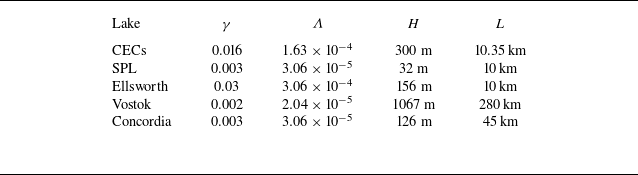
Table of the estimated slope $\gamma$
, and associated
$\gamma$
, and associated $\varLambda$
for five well-known SLs, CECs (named after the Chilean Centro de Estudios Científicos research centre), SPL (South Pole Lake), Ellsworth, Vostok and Concordia, discussed in Couston & Siegert (Reference Couston and Siegert2021) and Couston et al. (Reference Couston, Nandaha and Favier2022), using
$\varLambda$
for five well-known SLs, CECs (named after the Chilean Centro de Estudios Científicos research centre), SPL (South Pole Lake), Ellsworth, Vostok and Concordia, discussed in Couston & Siegert (Reference Couston and Siegert2021) and Couston et al. (Reference Couston, Nandaha and Favier2022), using $\lambda = {9.12\times 10^{-4}}\times \gamma$
as the estimate of the horizontal temperature gradient,
$\lambda = {9.12\times 10^{-4}}\times \gamma$
as the estimate of the horizontal temperature gradient, $k={0.56}\,{\,\textrm {W}\,\textrm {m}^{-1}\,\textrm {K}^{-1}}$
as the estimate for the thermal conductivity of water and
$k={0.56}\,{\,\textrm {W}\,\textrm {m}^{-1}\,\textrm {K}^{-1}}$
as the estimate for the thermal conductivity of water and $F={60}\,{\,\textrm {mW}\,\textrm {m}^{-2}}$
as the estimate of the average geothermal flux.
$F={60}\,{\,\textrm {mW}\,\textrm {m}^{-2}}$
as the estimate of the average geothermal flux.
The lake geometry controls the SL hydrodynamics at leading order. Subglacial lakes are subject to geothermal heat fluxes, of the order of 60 $\,\textrm {mW}\,\textrm {m}^{-2}$
across Antarctica (Martos et al. Reference Martos, Catalán, Jordan, Golynsky, Golynsky, Eagles and Vaughan2017) – with low heterogeneity at SL scales – which drive vertical flows whose intensity primarily depends on water depth (Couston & Siegert Reference Couston and Siegert2021). They are also subject to quasi-horizontal flows along the ice–water interface, when the interface is tilted and owing to the pressure dependence of the freezing point (Thoma et al. Reference Thoma, Grosfeld, Mayer, Smith, Woodward and Ross2011). These flows intensify as the interface length increases. The influence of geothermal heating (combined with depth) and interface tilt (combined with length) on the SL hydrodynamics can be quantified through two key dimensionless parameters, which are the flux Rayleigh number
$\,\textrm {mW}\,\textrm {m}^{-2}$
across Antarctica (Martos et al. Reference Martos, Catalán, Jordan, Golynsky, Golynsky, Eagles and Vaughan2017) – with low heterogeneity at SL scales – which drive vertical flows whose intensity primarily depends on water depth (Couston & Siegert Reference Couston and Siegert2021). They are also subject to quasi-horizontal flows along the ice–water interface, when the interface is tilted and owing to the pressure dependence of the freezing point (Thoma et al. Reference Thoma, Grosfeld, Mayer, Smith, Woodward and Ross2011). These flows intensify as the interface length increases. The influence of geothermal heating (combined with depth) and interface tilt (combined with length) on the SL hydrodynamics can be quantified through two key dimensionless parameters, which are the flux Rayleigh number $ \textit{Ra}_F$
and horizontal Rayleigh number
$ \textit{Ra}_F$
and horizontal Rayleigh number $ \textit{Ra}_L$
. In the case of SL, the horizontal Rayleigh number can be rewritten
$ \textit{Ra}_L$
. In the case of SL, the horizontal Rayleigh number can be rewritten
 \begin{align} \textit{Ra}_L = \frac {g\alpha \beta \gamma L^4}{\nu \kappa }, \end{align}
where $L$
is the lake length,
$L$
is the lake length, $\gamma$
is the interface slope,
$\gamma$
is the interface slope, $\beta \approx 10^{-3}$
K m–1 is the rate of change of the freezing temperature with depth (linked to the pressure increase with depth),
$\beta \approx 10^{-3}$
K m–1 is the rate of change of the freezing temperature with depth (linked to the pressure increase with depth), $k$
is thermal conductivity of the fluid and
$k$
is thermal conductivity of the fluid and $\nu$
and
$\nu$
and $\kappa$
are viscosity and thermal diffusivity. The fluid properties are described by the Prandtl number
$\kappa$
are viscosity and thermal diffusivity. The fluid properties are described by the Prandtl number $ \textit{Pr}= {\nu }/{\kappa }$
, approximately
$ \textit{Pr}= {\nu }/{\kappa }$
, approximately $O(10)$
in SLs (Couston Reference Couston2021). The shape of the lake is described by the aspect ratio
$O(10)$
in SLs (Couston Reference Couston2021). The shape of the lake is described by the aspect ratio $\varGamma = {L}/{H}$
. We note that most lakes can be considered fresh (Couston & Siegert Reference Couston and Siegert2021). The water depth, the length and the ice–water interface tilt of SLs vary greatly across cases. Subglacial lakes can be only 10 m deep and few hundreds of metres long, but also 1 km deep and hundreds of kilometres long, while the ice–water interface tilt can be close to 0 or up to few per cent (Couston, Nandaha & Favier Reference Couston, Nandaha and Favier2022). As a result, the range of dimensionless control parameters of interest to SL hydrodynamics research is broad, i.e. with
$\varGamma = {L}/{H}$
. We note that most lakes can be considered fresh (Couston & Siegert Reference Couston and Siegert2021). The water depth, the length and the ice–water interface tilt of SLs vary greatly across cases. Subglacial lakes can be only 10 m deep and few hundreds of metres long, but also 1 km deep and hundreds of kilometres long, while the ice–water interface tilt can be close to 0 or up to few per cent (Couston, Nandaha & Favier Reference Couston, Nandaha and Favier2022). As a result, the range of dimensionless control parameters of interest to SL hydrodynamics research is broad, i.e. with $ \textit{Ra}_F\in [10^{10},\; 10^{20}]$
and
$ \textit{Ra}_F\in [10^{10},\; 10^{20}]$
and $ \textit{Ra}_L\in [0,\; 10^{25}]$
and
$ \textit{Ra}_L\in [0,\; 10^{25}]$
and $\varGamma \geq 1$
(Couston & Siegert Reference Couston and Siegert2021).
$\varGamma \geq 1$
(Couston & Siegert Reference Couston and Siegert2021).
The ratio $\varLambda$
weighs the relative strength of HC and RBC
$\varLambda$
weighs the relative strength of HC and RBC
 \begin{align} \varLambda = \frac {\lambda k}{F}, \end{align}
where $\lambda = \beta \gamma$
is the temperature gradient on the top boundary. It can be interpreted as the ratio of the conductive horizontal flux and the conductive vertical flux at the top boundary
$\lambda = \beta \gamma$
is the temperature gradient on the top boundary. It can be interpreted as the ratio of the conductive horizontal flux and the conductive vertical flux at the top boundary
 \begin{align} \varLambda = \frac {{\left ( \partial T / \partial x\right )}}{{\left ( \partial T / \partial z\right )}}, \end{align}
where the partial derivatives are computed at the boundary where the fluid is quiescent (no slip). The vertical heat flux, $k\partial T/\partial z$
, must be equal to
$k\partial T/\partial z$
, must be equal to $F$
on average in the stationary state.
$F$
on average in the stationary state.
One major challenge is to determine the flow structure in the system for a given value of $\varLambda$
. The numerical simulations of Couston et al. (Reference Couston, Nandaha and Favier2022) demonstrated a hysteretic behaviour of this model system near
$\varLambda$
. The numerical simulations of Couston et al. (Reference Couston, Nandaha and Favier2022) demonstrated a hysteretic behaviour of this model system near $\varLambda \approx {10^{-2}}$
at relatively low Rayleigh numbers (
$\varLambda \approx {10^{-2}}$
at relatively low Rayleigh numbers ( $ \textit{Ra}_F \in [ {10^6}; {10^8} ]$
) and
$ \textit{Ra}_F \in [ {10^6}; {10^8} ]$
) and $ \textit{Pr}=1$
, and several aspect ratios (4, 8, 12 and 16). The range of
$ \textit{Pr}=1$
, and several aspect ratios (4, 8, 12 and 16). The range of $\varLambda$
in nature is expected to be much smaller than
$\varLambda$
in nature is expected to be much smaller than $10^{-2}$
, see table 1. Therefore, the numerical results suggest that the dynamics of SLs should be dominated by vertical, Rayleigh–Bénard-like, convective motions.
$10^{-2}$
, see table 1. Therefore, the numerical results suggest that the dynamics of SLs should be dominated by vertical, Rayleigh–Bénard-like, convective motions.
The objective of the work presented in this paper is to operate a simple experimental model of SLs, with $ \textit{Ra}_F={10^9}$
and
$ \textit{Ra}_F={10^9}$
and $ \textit{Pr}=7$
, i.e. close to the values of Couston et al. (Reference Couston, Nandaha and Favier2022), but paving the way for more realistic values in future experimental works, including notably higher
$ \textit{Pr}=7$
, i.e. close to the values of Couston et al. (Reference Couston, Nandaha and Favier2022), but paving the way for more realistic values in future experimental works, including notably higher $ \textit{Pr}$
and a three-dimensional dynamics. This flux Rayleigh number is obtained with an heating power of 100 W, corresponding to a heat-flux 2.28
$ \textit{Pr}$
and a three-dimensional dynamics. This flux Rayleigh number is obtained with an heating power of 100 W, corresponding to a heat-flux 2.28 $\,\textrm {kW}\,\textrm {m}^{-2}$
. The Rayleigh number at
$\,\textrm {kW}\,\textrm {m}^{-2}$
. The Rayleigh number at $\varLambda = 0$
in this configuration is
$\varLambda = 0$
in this configuration is $5.4\times 10^7$
. The flow is characterised for various values of
$5.4\times 10^7$
. The flow is characterised for various values of $\varLambda$
, a threshold value is inferred from the change in the mean flow pattern and a hysteretic behaviour is demonstrated.
$\varLambda$
, a threshold value is inferred from the change in the mean flow pattern and a hysteretic behaviour is demonstrated.
2. Experimental set-up
Schematic of the experimental cell. Here, $T_1, \ldots , T_6$
are PT-100 sensors inserted into the top plate,
$T_1, \ldots , T_6$
are PT-100 sensors inserted into the top plate, $B_1, B_2, B_3$
are PT-100 sensors inserted into the bottom plate and
$B_1, B_2, B_3$
are PT-100 sensors inserted into the bottom plate and $p_1, p_2, p_3$
are sensors that can be inserted into the cell to obtain temperature profiles in the bulk of the flow. The blue to red shading indicates the direction of the temperature gradient (warmer on the right).
$p_1, p_2, p_3$
are sensors that can be inserted into the cell to obtain temperature profiles in the bulk of the flow. The blue to red shading indicates the direction of the temperature gradient (warmer on the right).
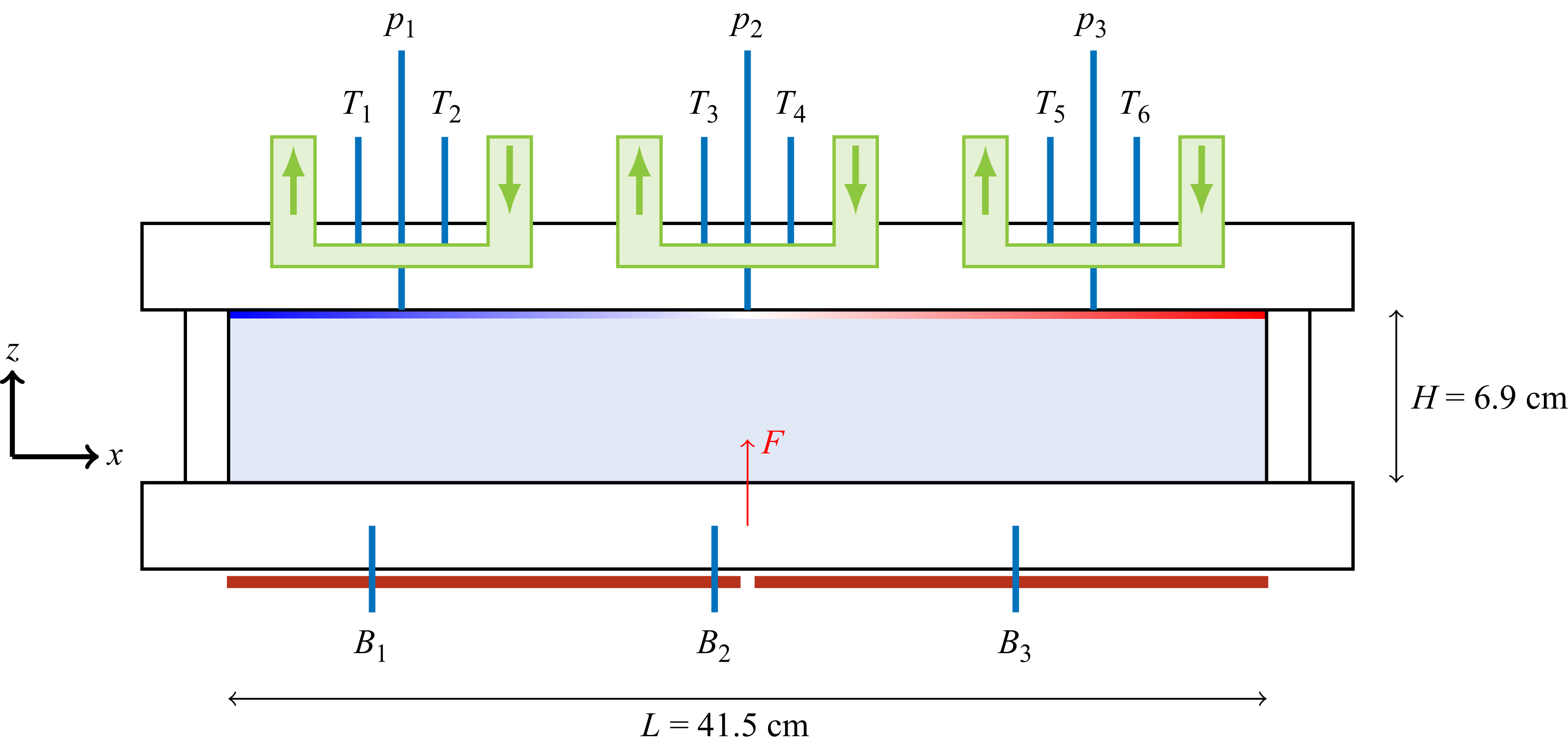
Our experimental set-up consists in a modified RBC cell where a horizontal temperature gradient is imposed on the top boundary. The cell dimensions are $L\times H\times D = {41.5{\,\textrm {cm}}\times 6.9{\,\textrm {cm}}\times 10.5{\,\textrm {cm}}}$
, where
$L\times H\times D = {41.5{\,\textrm {cm}}\times 6.9{\,\textrm {cm}}\times 10.5{\,\textrm {cm}}}$
, where $L$
is the width,
$L$
is the width, $H$
is the height and
$H$
is the height and $D$
is the depth of the cell. The aspect ratio,
$D$
is the depth of the cell. The aspect ratio, $\varGamma = L/H$
is 6. We consider only one aspect ratio in this work, as exploring values of
$\varGamma = L/H$
is 6. We consider only one aspect ratio in this work, as exploring values of $\varGamma$
experimentally requires building several cells. In the numerical simulations of Couston et al. (Reference Couston, Nandaha and Favier2022), the transition threshold does not depend on
$\varGamma$
experimentally requires building several cells. In the numerical simulations of Couston et al. (Reference Couston, Nandaha and Favier2022), the transition threshold does not depend on $\varGamma$
. The value
$\varGamma$
. The value $\varGamma =6$
was chosen to be large enough to have several rolls in the RBC regime, while keeping
$\varGamma =6$
was chosen to be large enough to have several rolls in the RBC regime, while keeping $H$
large enough to reach high
$H$
large enough to reach high $ \textit{Ra}_F$
with our existing plate of length
$ \textit{Ra}_F$
with our existing plate of length $L={41.5}\,\textrm {cm}$
.
$L={41.5}\,\textrm {cm}$
.
The working fluid is deionised water at an average temperature of ${20}{\,^\circ\textrm {C}}$
(
${20}{\,^\circ\textrm {C}}$
( $ \textit{Pr} = 7$
). The temperature in the cell is always larger than 4
$ \textit{Pr} = 7$
). The temperature in the cell is always larger than 4 $\,^\circ\textrm {C}$
, so we do not have the density anomaly of water. This would correspond to SLs under thick ice, for which the pressure is high enough that water no longer has a density anomaly (Couston & Siegert Reference Couston and Siegert2021). The top and bottom plates are made of aluminium alloy (5083) and anodised in black. The sidewalls are made of glass. Glass is chosen for the walls for their good optical quality, in particular they do not induce gradients of optical index when submitted to a temperature difference. However, they are not very good insulators. To avoid spurious heat losses through the lateral walls, the working temperature of the cell is chosen to match the temperature of the room. The correction of the Nusselt number due to conduction across the glass walls can be evaluated in the Rayleigh–Bénard case with well-established models of the literature (Ahlers Reference Ahlers2000; Roche et al. Reference Roche, Castaing, Chabaud, Hébral and Sommeria2001), and it yields a correction of order 10 %, which we will not consider in the following.
$\,^\circ\textrm {C}$
, so we do not have the density anomaly of water. This would correspond to SLs under thick ice, for which the pressure is high enough that water no longer has a density anomaly (Couston & Siegert Reference Couston and Siegert2021). The top and bottom plates are made of aluminium alloy (5083) and anodised in black. The sidewalls are made of glass. Glass is chosen for the walls for their good optical quality, in particular they do not induce gradients of optical index when submitted to a temperature difference. However, they are not very good insulators. To avoid spurious heat losses through the lateral walls, the working temperature of the cell is chosen to match the temperature of the room. The correction of the Nusselt number due to conduction across the glass walls can be evaluated in the Rayleigh–Bénard case with well-established models of the literature (Ahlers Reference Ahlers2000; Roche et al. Reference Roche, Castaing, Chabaud, Hébral and Sommeria2001), and it yields a correction of order 10 %, which we will not consider in the following.
The temperature of the plates are measured with class 1/10 PT-100 sensors inserted into the aluminium plate: the bottom plate is fitted with three probes, $B_1$
,
$B_1$
, $B_2$
,
$B_2$
, $B_3$
, and the top plate with six probes,
$B_3$
, and the top plate with six probes, $T_1$
,
$T_1$
, $T_2$
,
$T_2$
, $T_3$
,
$T_3$
, $T_4$
,
$T_4$
, $T_5$
,
$T_5$
, $T_6$
, allowing us to estimate the horizontal temperature gradient at the top boundary. These probes are inserted inside the plate, at mid-height of the plate. A sketch of the cell is provided in figure 2.
$T_6$
, allowing us to estimate the horizontal temperature gradient at the top boundary. These probes are inserted inside the plate, at mid-height of the plate. A sketch of the cell is provided in figure 2.
Example of temperature readings from the sensors in the apparatus (a) with a small horizontal temperature gradient on the top plate and (b) with a large horizontal temperature gradient on the top plate.

Temperature inside the fluid is investigated by inserting temperature sensors inside the cell, at $x_1={4.55}\,\textrm {}$
,
$x_1={4.55}\,\textrm {}$
, $x_2={20.7}\,\textrm {}$
and
$x_2={20.7}\,\textrm {}$
and $x_3={36.95}\,\textrm {cm}$
, passing through three small tubes, shown as
$x_3={36.95}\,\textrm {cm}$
, passing through three small tubes, shown as $p_1$
,
$p_1$
, $p_2$
and
$p_2$
and $p_3$
in figure 2. The probes are 2 mm-wide class 1/3 PT-100 sensors, which can be moved along the vertical axis. The vertical positions of the probes are pinpointed optically with the camera. When they are no longer used, they are then removed from the field of view. In particular, they can be moved as close as possible to the plate, in order to measure the horizontal gradient close to the top boundary. However, they are always well outside the thermal boundary layer. In the condition where a gradient is imposed at the plate, these sensors evidence the horizontal temperature gradient in the fluid, see figure 3.
$p_3$
in figure 2. The probes are 2 mm-wide class 1/3 PT-100 sensors, which can be moved along the vertical axis. The vertical positions of the probes are pinpointed optically with the camera. When they are no longer used, they are then removed from the field of view. In particular, they can be moved as close as possible to the plate, in order to measure the horizontal gradient close to the top boundary. However, they are always well outside the thermal boundary layer. In the condition where a gradient is imposed at the plate, these sensors evidence the horizontal temperature gradient in the fluid, see figure 3.
The control parameters are: the imposed heat flux on the bottom plate, $F$
, the average temperature of the top plate,
$F$
, the average temperature of the top plate, $ \langle T_{\textit{top}} \rangle$
, and the horizontal temperature gradient on the top plate,
$ \langle T_{\textit{top}} \rangle$
, and the horizontal temperature gradient on the top plate, $\lambda$
, which is imposed at constant
$\lambda$
, which is imposed at constant $ \langle T_{\textit{top}} \rangle$
. Or, in non-dimensional terms,
$ \langle T_{\textit{top}} \rangle$
. Or, in non-dimensional terms, $ \textit{Ra}_F$
,
$ \textit{Ra}_F$
, $ \textit{Ra}_L$
and
$ \textit{Ra}_L$
and $\varLambda$
. Since the aspect ratio
$\varLambda$
. Since the aspect ratio $\varGamma$
is fixed in our experiment, there are only two independent non-dimensional control parameters,
$\varGamma$
is fixed in our experiment, there are only two independent non-dimensional control parameters, $ \textit{Ra}_F$
and
$ \textit{Ra}_F$
and $ \textit{Ra}_L$
or
$ \textit{Ra}_L$
or $\varLambda$
. The temperature of the bottom plate is not imposed, and its value depends on the heat transfer efficiency. In the following, the efficiency of the heat transport from the bottom to the top plate is estimated with the Nusselt number, which simply writes, in the experimental case, as
$\varLambda$
. The temperature of the bottom plate is not imposed, and its value depends on the heat transfer efficiency. In the following, the efficiency of the heat transport from the bottom to the top plate is estimated with the Nusselt number, which simply writes, in the experimental case, as
 \begin{align} \textit{Nu} = \frac {\textit{FH}}{k \left ( \langle T_{{bottom}} \rangle - \langle T_{\textit{top}} \rangle \right )}, \end{align}
where $ \langle T_{\textit{top}} \rangle$
and
$ \langle T_{\textit{top}} \rangle$
and $ \langle T_{{bottom}} \rangle$
are both temporal and spatial averages. The heat flux on the bottom boundary is imposed by heating with two 4 in. × 8 in. silicone heater mats with a maximum power of 160 W each. The top plate is cooled with three independent circulations of a mixture of water and ethylene-glycol, flowing into tight meanders machined at the top of the plate, and regulated by three independent chillers.
$ \langle T_{{bottom}} \rangle$
are both temporal and spatial averages. The heat flux on the bottom boundary is imposed by heating with two 4 in. × 8 in. silicone heater mats with a maximum power of 160 W each. The top plate is cooled with three independent circulations of a mixture of water and ethylene-glycol, flowing into tight meanders machined at the top of the plate, and regulated by three independent chillers.
Two examples of temperature readings are shown in figure 3. An example with a small temperature gradient is shown in figure 3(a). The temperature of the bottom plate that is not controlled is larger than that of the top plate due to the bottom heat flux $F$
. The horizontal temperature gradient from the
$F$
. The horizontal temperature gradient from the $p_1$
,
$p_1$
, $p_2$
,
$p_2$
, $p_3$
probes at
$p_3$
probes at $z={6.4}\,\textrm {cm}$
is close to the gradient from the
$z={6.4}\,\textrm {cm}$
is close to the gradient from the $T_1, \ldots , T_6$
probes inside the top plate. For our largest horizontal temperature gradient (figure 3
b), the warmest part of the top plate has roughly the same temperature as the bottom plate. Each pair of thermometers in the top plate (
$T_1, \ldots , T_6$
probes inside the top plate. For our largest horizontal temperature gradient (figure 3
b), the warmest part of the top plate has roughly the same temperature as the bottom plate. Each pair of thermometers in the top plate ( $T_1$
and
$T_1$
and $T_2$
,
$T_2$
, $T_3$
and
$T_3$
and $T_4$
,
$T_4$
, $T_5$
and
$T_5$
and $T_6$
) is located right below the cooling meander and reveal steps, which would be partly smoothed out at the boundary with the fluid because of thermal diffusion inside the plate. However, the precise horizontal profile at the boundary cannot be measured. Our set-up does not guarantee a purely linear gradient, but this should not be an issue, since Ding et al. (Reference Ding, Chong and Xia2021) showed that the details of the horizontal profile seldom impact the heat fluxes.
$T_6$
) is located right below the cooling meander and reveal steps, which would be partly smoothed out at the boundary with the fluid because of thermal diffusion inside the plate. However, the precise horizontal profile at the boundary cannot be measured. Our set-up does not guarantee a purely linear gradient, but this should not be an issue, since Ding et al. (Reference Ding, Chong and Xia2021) showed that the details of the horizontal profile seldom impact the heat fluxes.
In practice, we chose one value of $F = {0.23}{\,\textrm {W}\,\textrm {cm}^{-2}}$
for all the experiments discussed in this paper, corresponding to a flux Rayleigh number,
$F = {0.23}{\,\textrm {W}\,\textrm {cm}^{-2}}$
for all the experiments discussed in this paper, corresponding to a flux Rayleigh number, $ \textit{Ra}_F = {1.3\times 10^9}$
, and we fixed
$ \textit{Ra}_F = {1.3\times 10^9}$
, and we fixed $ \langle T_{\textit{top}} \rangle = {15}{\,^\circ\textrm {C}}$
. We varied
$ \langle T_{\textit{top}} \rangle = {15}{\,^\circ\textrm {C}}$
. We varied $\lambda$
, starting from a vanishingly small value (homogeneous temperature on the top plate, within the experimental accuracy), and increasing the gradient until a maximum value of 484 mK cm–1. Then we decreased the gradient gradually, back to the smallest possible value. The setpoints are summarised in table 2. Several measurements are run with mostly similar conditions, over several days, before changing the setpoint, but are omitted from the table for clarity. Increasing or decreasing
$\lambda$
, starting from a vanishingly small value (homogeneous temperature on the top plate, within the experimental accuracy), and increasing the gradient until a maximum value of 484 mK cm–1. Then we decreased the gradient gradually, back to the smallest possible value. The setpoints are summarised in table 2. Several measurements are run with mostly similar conditions, over several days, before changing the setpoint, but are omitted from the table for clarity. Increasing or decreasing $\lambda$
is done by changing the setpoint on the chillers that control the temperature of the cooling fluid in the meanders of the top plate, then waiting several hours, typically overnight, to allow for the development of the statistically stationary state in the cell. Then, series of video recordings are acquired, as well as vertical temperature profiles by moving the sensors
$\lambda$
is done by changing the setpoint on the chillers that control the temperature of the cooling fluid in the meanders of the top plate, then waiting several hours, typically overnight, to allow for the development of the statistically stationary state in the cell. Then, series of video recordings are acquired, as well as vertical temperature profiles by moving the sensors $p_1$
,
$p_1$
, $p_2$
and
$p_2$
and $p_3$
on the vertical axis. The Rayleigh number
$p_3$
on the vertical axis. The Rayleigh number $ \textit{Ra}$
, and Nusselt number
$ \textit{Ra}$
, and Nusselt number $ \textit{Nu}$
, in the table refer to the vertical heat transport. They are estimated with (1.1) and (1.4), using the average temperature of the plates. The full Nusselt number in horizontal or mixed conditions, defined from (1.3), is not accessible experimentally. It is interesting to note that the (vertical) Nusselt number is not modified by the horizontal temperature gradient,
$ \textit{Nu}$
, in the table refer to the vertical heat transport. They are estimated with (1.1) and (1.4), using the average temperature of the plates. The full Nusselt number in horizontal or mixed conditions, defined from (1.3), is not accessible experimentally. It is interesting to note that the (vertical) Nusselt number is not modified by the horizontal temperature gradient, $\lambda$
, even at our highest gradient. Even in the regime with the strongest HC influence, the efficiency of the vertical heat transport is still that of pure RBC. It may not be a surprise as the horizontal heat transport remains much smaller than the vertical heat transport (
$\lambda$
, even at our highest gradient. Even in the regime with the strongest HC influence, the efficiency of the vertical heat transport is still that of pure RBC. It may not be a surprise as the horizontal heat transport remains much smaller than the vertical heat transport ( $\varLambda \ll 1$
), even though
$\varLambda \ll 1$
), even though $ \textit{Ra}_L \gt Ra$
, which might derive from the fact that pure HC is non-turbulent (Paparella & Young Reference Paparella and Young2002), and the HC Nusselt number scales like
$ \textit{Ra}_L \gt Ra$
, which might derive from the fact that pure HC is non-turbulent (Paparella & Young Reference Paparella and Young2002), and the HC Nusselt number scales like $ \textit{Ra}_L^{1/5}$
(Rossby Reference Rossby1965). Therefore, HC driving would need to have a much higher
$ \textit{Ra}_L^{1/5}$
(Rossby Reference Rossby1965). Therefore, HC driving would need to have a much higher $ \textit{Ra}_L$
to overcome the heat efficiency of vertical convection for which the Nusselt number scales typically as
$ \textit{Ra}_L$
to overcome the heat efficiency of vertical convection for which the Nusselt number scales typically as $ \textit{Ra}^{1/3}$
.
$ \textit{Ra}^{1/3}$
.
Operating conditions in the experiment. The control parameters are the heat flux on the bottom plate, $F$
(and therefore
$F$
(and therefore $ \textit{Ra}_F$
), and the temperatures of the top plate: the mean temperature
$ \textit{Ra}_F$
), and the temperatures of the top plate: the mean temperature $\langle T_{\textit{top}}\rangle$
and the horizontal temperature gradient
$\langle T_{\textit{top}}\rangle$
and the horizontal temperature gradient $\lambda$
(and therefore the horizontal Rayleigh number
$\lambda$
(and therefore the horizontal Rayleigh number $ \textit{Ra}_L$
), as well as
$ \textit{Ra}_L$
), as well as $\varLambda = k\lambda /F$
. The system response determines the bottom temperature
$\varLambda = k\lambda /F$
. The system response determines the bottom temperature $\langle T_{{bot}}\rangle$
(and therefore the vertical temperature difference,
$\langle T_{{bot}}\rangle$
(and therefore the vertical temperature difference, $\Delta T$
), and the flow structure (number of rolls
$\Delta T$
), and the flow structure (number of rolls $N$
and mean flow velocity expressed as the Reynolds number
$N$
and mean flow velocity expressed as the Reynolds number $Re$
). Formally, both
$Re$
). Formally, both $ \textit{Ra}$
and
$ \textit{Ra}$
and $ \textit{Nu}$
are responses, in the sense that they depend on
$ \textit{Nu}$
are responses, in the sense that they depend on $\Delta T$
, which is not controlled.
$\Delta T$
, which is not controlled.
The flow is visualised with shadowgraph with a simple diverging light optical set up (Settles Reference Settles2001), similar to that of Belkadi et al. (Reference Belkadi, Guislain, Sergent, Podvin, Chillà and Salort2020). The light source is a monochromatic light emitting diode at 450 nm with output power 1850 mW with an iris diaphragm to further reduce the spatial extent of the light source. Images are recorded for one hour with a PCO-1600 monochrome camera with an exposure time 15 ms and a frame rate of 15 fps. Examples of shadowgraph images are shown in figure 4. Because we use a simple direct shadowgraphy set up, the raw images from the camera are inhomogeneous: there is more light at the centre (which is in the direct line of sight of the light source). This does not cause an issue because the PCO-1600 camera has a dynamic range of 14 bits, so it remains sensitive enough both at the centre and on the edge of the image. The instantaneous shadowgraph images are recovered by normalising the raw images $I(x, z, t)$
by the average illumination
$I(x, z, t)$
by the average illumination $I_0(x, z)$
. As discussed by Belkadi et al. (Reference Belkadi, Guislain, Sergent, Podvin, Chillà and Salort2020), one practical means to obtain
$I_0(x, z)$
. As discussed by Belkadi et al. (Reference Belkadi, Guislain, Sergent, Podvin, Chillà and Salort2020), one practical means to obtain $I_0(x, z)$
is to simply average the raw images in time. Indeed, thermal plumes produce a pattern with both brighter than average and darker then average parts at their boundary, the plume patterns cancel out on average, and the remaining image is an estimate for the mean illumination. The colour bar in the figure indicates pixels brighter than average (
$I_0(x, z)$
is to simply average the raw images in time. Indeed, thermal plumes produce a pattern with both brighter than average and darker then average parts at their boundary, the plume patterns cancel out on average, and the remaining image is an estimate for the mean illumination. The colour bar in the figure indicates pixels brighter than average ( $I(x, z, t) / I_0 \gt 1$
) or darker than average (
$I(x, z, t) / I_0 \gt 1$
) or darker than average ( $I(x, z, t) / I_0 \lt 1$
).
$I(x, z, t) / I_0 \lt 1$
).
The shadowgraph pattern is the result of the path of light in the refractive index field. The image projected on the screen is determined, at leading order, by the second derivative of the refractive index (Settles Reference Settles2001)
 \begin{align} \frac {I(x, z, t)}{I_0(x, z)} = \frac {\gamma (\eta -\gamma )}{\eta }\int _{0}^{D}\left ( \frac {\partial ^2}{\partial x^2} + \frac {\partial ^2}{\partial z^2}\right )\left ( \ln {n} \right )\mathrm{d}y , \end{align}
where $\gamma$
is the distance between the cell and the projection screen, and
$\gamma$
is the distance between the cell and the projection screen, and $\eta$
is the distance between the light source and the projection screen. In Boussinesq conditions, the variations of the refractive index,
$\eta$
is the distance between the light source and the projection screen. In Boussinesq conditions, the variations of the refractive index, $\mathrm{d}n$
, are proportional to the variations of density,
$\mathrm{d}n$
, are proportional to the variations of density, $\mathrm{d}\rho$
, themselves proportional to the variations of temperature
$\mathrm{d}\rho$
, themselves proportional to the variations of temperature $\mathrm{d}T$
(Jenkins Reference Jenkins1988).
$\mathrm{d}T$
(Jenkins Reference Jenkins1988).
3. Flow structure and velocity estimates
Instantaneous shadowgraph images for $ \textit{Ra}_F = {10^9}$
and
$ \textit{Ra}_F = {10^9}$
and $ \textit{Pr} = {6.8}$
. The vertical temperature difference is 10 K. (a) No horizontal temperature gradient (pure RBC), three convection rolls; (b) intermediate regime with a moderate horizontal temperature difference (0.6 K) showing two convection rolls; (c) large horizontal temperature difference (20 K across the plate width), one large roll (HC-influenced regime).
$ \textit{Pr} = {6.8}$
. The vertical temperature difference is 10 K. (a) No horizontal temperature gradient (pure RBC), three convection rolls; (b) intermediate regime with a moderate horizontal temperature difference (0.6 K) showing two convection rolls; (c) large horizontal temperature difference (20 K across the plate width), one large roll (HC-influenced regime).
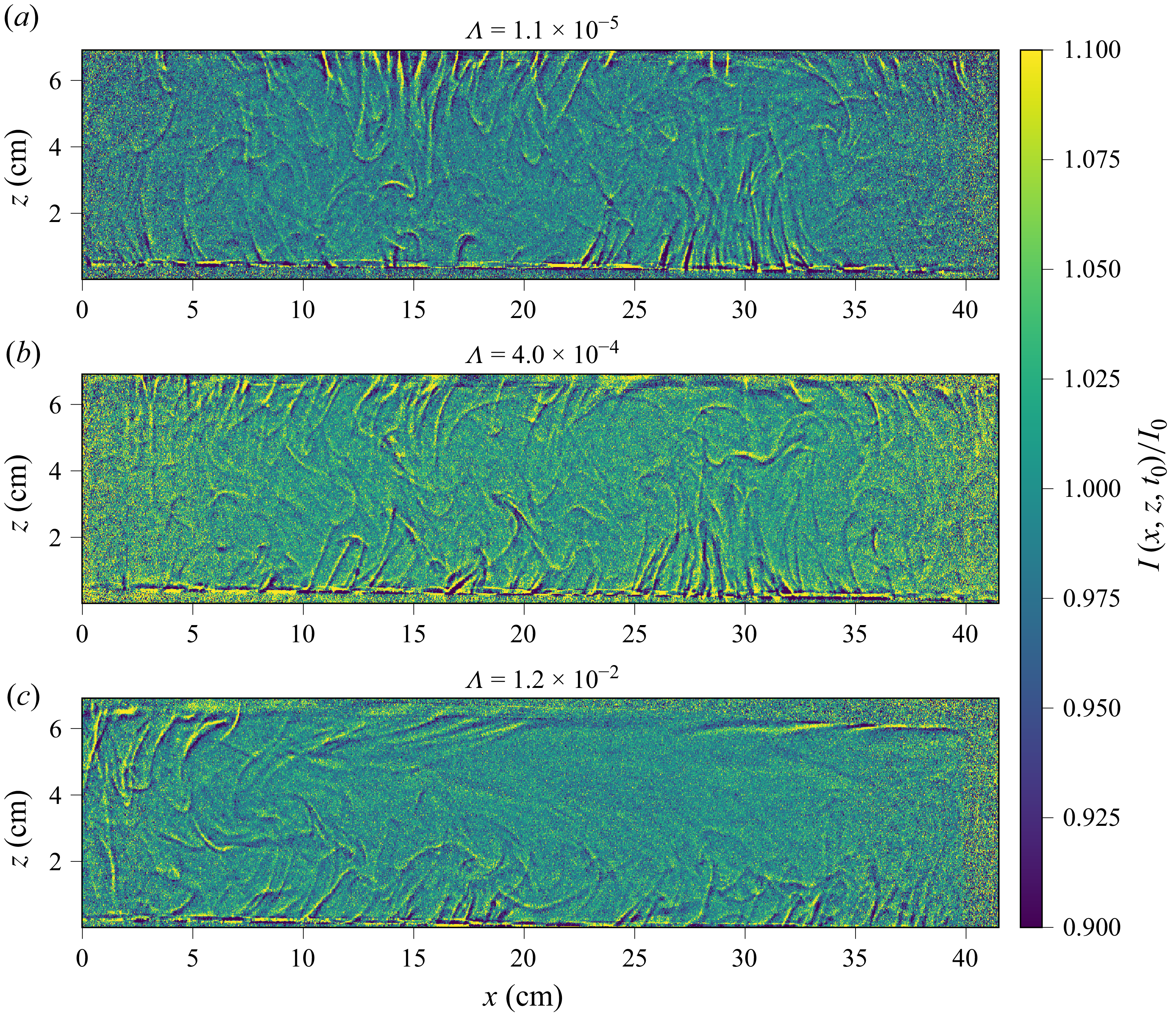
We follow the analysis of Couston et al. (Reference Couston, Nandaha and Favier2022), and aim to use the number of convection rolls as a proxy of the main convective mechanism: when RBC is dominant, the LSC organises in the form of several convection cells of identical size; when HC is dominant, the LSC is one large asymmetrical roll with its orientation fixed by the direction of the horizontal temperature gradient. In the latter case, there is a layer of fluid, below the warm side of the top plate, where temperature remains stably stratified. The flow organisation is visible in the shadowgraph pattern, shown in figure 4. Note that the upwelling plumes at $x=0$
and the downwelling plumes at
$x=0$
and the downwelling plumes at $x={41.5}\,\textrm {cm}$
are not very well resolved due to light reflection very close to the walls. The expected flow structure in RBC, for moderate aspect ratios close to that used in this study (
$x={41.5}\,\textrm {cm}$
are not very well resolved due to light reflection very close to the walls. The expected flow structure in RBC, for moderate aspect ratios close to that used in this study ( $\varGamma =6$
), always consists of more than one roll. In particular, Sergent & Le Quéré (Reference Sergent and Le Quéré2011) find that the LSC structure in their
$\varGamma =6$
), always consists of more than one roll. In particular, Sergent & Le Quéré (Reference Sergent and Le Quéré2011) find that the LSC structure in their $\varGamma =5$
cell may have 2, 3 or 4 rolls, with spontaneous transitions between the flow states on long time scales. They do not observe a flow structure with only 1 roll.
$\varGamma =5$
cell may have 2, 3 or 4 rolls, with spontaneous transitions between the flow states on long time scales. They do not observe a flow structure with only 1 roll.
In the pure RBC case ( $\varLambda = 0$
, figure 4
a), upwelling plumes are visible above the bottom plate near
$\varLambda = 0$
, figure 4
a), upwelling plumes are visible above the bottom plate near $x={30}\,\textrm {cm}$
, and downwelling plumes are visible below the top plate near
$x={30}\,\textrm {cm}$
, and downwelling plumes are visible below the top plate near $x={15}\,\textrm {cm}$
. This corresponds to a flow structure with three convection rolls, similar to the flow structure observed by Sergent & Le Quéré (Reference Sergent and Le Quéré2011) in turbulent RBC with a similar geometry. They are not visible in the case of
$x={15}\,\textrm {cm}$
. This corresponds to a flow structure with three convection rolls, similar to the flow structure observed by Sergent & Le Quéré (Reference Sergent and Le Quéré2011) in turbulent RBC with a similar geometry. They are not visible in the case of $\varLambda = {1.25\times 10^{-2}}$
(figure 4
c) where HC is dominant. Plumes near the bottom plate travel from left to right along the full width of the cell. Downwelling plumes are visible at
$\varLambda = {1.25\times 10^{-2}}$
(figure 4
c) where HC is dominant. Plumes near the bottom plate travel from left to right along the full width of the cell. Downwelling plumes are visible at $x=0$
. The asymmetry between top and bottom is clearly visible. The intermediate case (
$x=0$
. The asymmetry between top and bottom is clearly visible. The intermediate case ( $\varLambda = {4\times 10^{-4}}$
, figure 4
b) is closer to the RBC case, with plumes observed on both plates. The upwelling plumes at
$\varLambda = {4\times 10^{-4}}$
, figure 4
b) is closer to the RBC case, with plumes observed on both plates. The upwelling plumes at $x={27.5}\,\textrm {cm}$
highlights the two convection rolls: one large roll on the left, and a smaller roll on the right. Note that the configuration with the large roll on the right and the smaller roll on the left has also been observed in our system. In both cases, the larger roll is the one turning counter-clockwise, i.e. in the same direction as the single large roll observed in the HC-dominant case.
$x={27.5}\,\textrm {cm}$
highlights the two convection rolls: one large roll on the left, and a smaller roll on the right. Note that the configuration with the large roll on the right and the smaller roll on the left has also been observed in our system. In both cases, the larger roll is the one turning counter-clockwise, i.e. in the same direction as the single large roll observed in the HC-dominant case.
Space–time diagram obtained from the sequence of shadowgraph images for $\varLambda = 0$
at
$\varLambda = 0$
at $z_0 = {5.9}\,\textrm {cm}$
(close to the top plate). Only one minute is plotted for readability.
$z_0 = {5.9}\,\textrm {cm}$
(close to the top plate). Only one minute is plotted for readability.
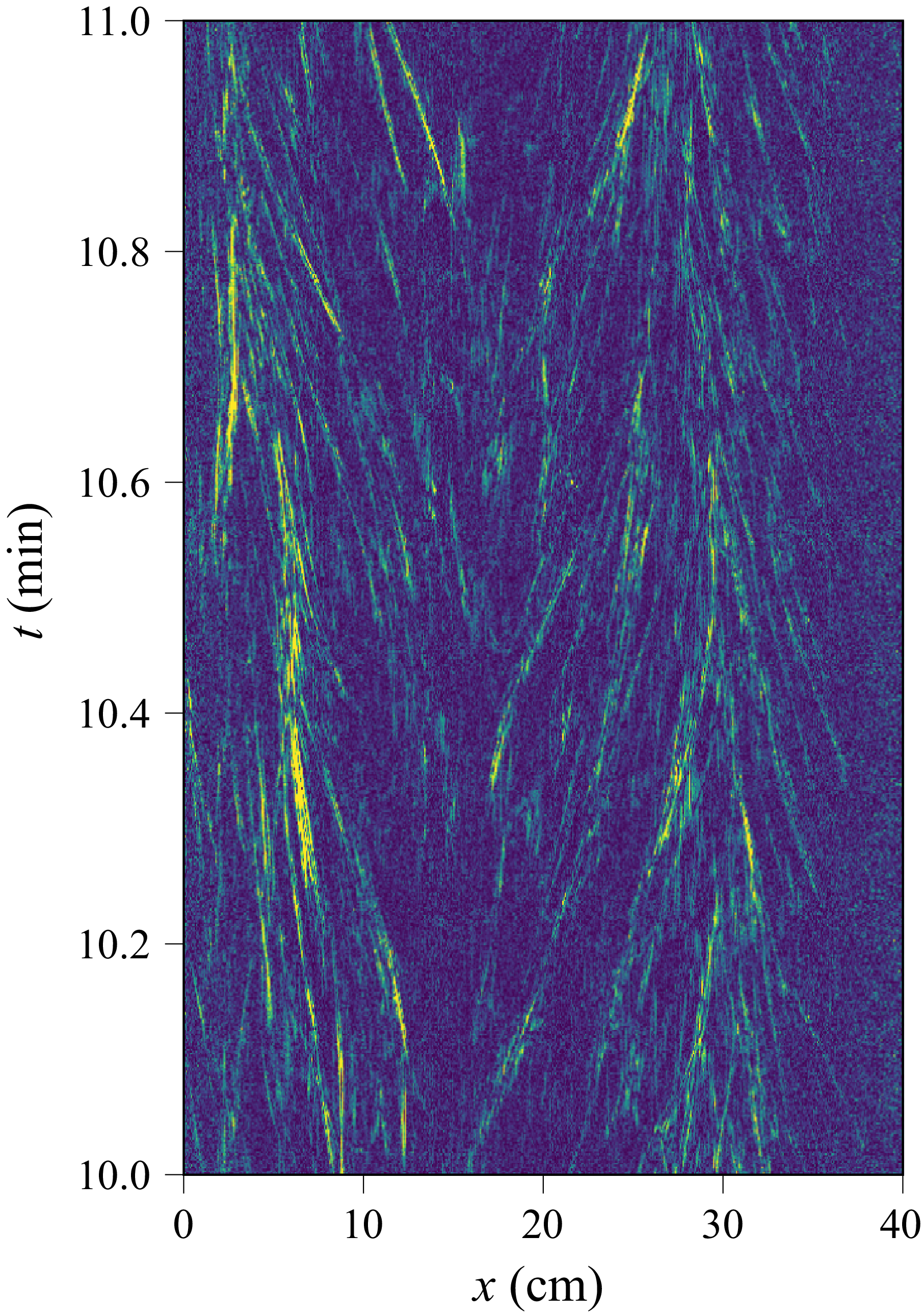
There are several methods to infer velocity components from the sequence of shadowgraph images, $I(x, z, t)$
: using optical flow (Crone, McDuff & Wilcock Reference Crone, McDuff and Wilcock2008), correlation image velocimetry (McConnochie & Kerr Reference McConnochie and Kerr2016; Brichet et al. Reference Brichet, Carbonneau, Bernard, Braun, Méthivier, Fraigneau, Lucor, Chillà, Sergent and Salort2025) or spatio-temporal diagrams (Belkadi et al. Reference Belkadi, Guislain, Sergent, Podvin, Chillà and Salort2020; Méthivier et al. Reference Méthivier, Braun, Chillà and Salort2021). In this work, we use spatio-temporal diagrams, similarly to Belkadi et al. (Reference Belkadi, Guislain, Sergent, Podvin, Chillà and Salort2020). A space–time diagram is obtained by selecting an horizontal line at a given
$I(x, z, t)$
: using optical flow (Crone, McDuff & Wilcock Reference Crone, McDuff and Wilcock2008), correlation image velocimetry (McConnochie & Kerr Reference McConnochie and Kerr2016; Brichet et al. Reference Brichet, Carbonneau, Bernard, Braun, Méthivier, Fraigneau, Lucor, Chillà, Sergent and Salort2025) or spatio-temporal diagrams (Belkadi et al. Reference Belkadi, Guislain, Sergent, Podvin, Chillà and Salort2020; Méthivier et al. Reference Méthivier, Braun, Chillà and Salort2021). In this work, we use spatio-temporal diagrams, similarly to Belkadi et al. (Reference Belkadi, Guislain, Sergent, Podvin, Chillà and Salort2020). A space–time diagram is obtained by selecting an horizontal line at a given $z_0$
, and showing
$z_0$
, and showing $I(x, z_0, t)$
as a two-dimensional image (see figure 5). In this image, thermal plumes moving horizontally produce lines. The slope of the line gives the plume velocity. The vertical velocity could also be inferred from a vertical line at a given
$I(x, z_0, t)$
as a two-dimensional image (see figure 5). In this image, thermal plumes moving horizontally produce lines. The slope of the line gives the plume velocity. The vertical velocity could also be inferred from a vertical line at a given $x_0$
. The lines are detected in this image with the line segment detector algorithm in the free OpenCV library (Bradski Reference Bradski2000), based on the algorithm of Grompone von Gioi et al. (Reference Grompone von Gioi, Jakubowicz, Morel and Randall2012).
$x_0$
. The lines are detected in this image with the line segment detector algorithm in the free OpenCV library (Bradski Reference Bradski2000), based on the algorithm of Grompone von Gioi et al. (Reference Grompone von Gioi, Jakubowicz, Morel and Randall2012).
Here, we choose two horizontal lines, at $z_0={0.4}\,\textrm {cm}$
(near the bottom boundary), and
$z_0={0.4}\,\textrm {cm}$
(near the bottom boundary), and $z_0={5.9}\,\textrm {cm}$
(near the top boundary), where the plume pattern is most visible (see figure 4), and plume advection yields a set of small lines at positions
$z_0={5.9}\,\textrm {cm}$
(near the top boundary), where the plume pattern is most visible (see figure 4), and plume advection yields a set of small lines at positions $x_i$
and times
$x_i$
and times $t_i$
in the spatio-temporal diagram. The slope of each line yields an estimate of the horizontal velocity
$t_i$
in the spatio-temporal diagram. The slope of each line yields an estimate of the horizontal velocity $u(x_i, z_0, t_i)$
. The set of velocities can then be averaged to obtain mean profiles
$u(x_i, z_0, t_i)$
. The set of velocities can then be averaged to obtain mean profiles $\bar {u}(x, z_0)$
.
$\bar {u}(x, z_0)$
.
Profiles of horizontal velocity $\bar {u}(x, z_0)$
, at fixed height
$\bar {u}(x, z_0)$
, at fixed height $z_0 = {5.9}\,\textrm {cm}$
(close to the top plate), and
$z_0 = {5.9}\,\textrm {cm}$
(close to the top plate), and $z_0={0.4}\,\textrm {cm}$
(close to the bottom plate), for
$z_0={0.4}\,\textrm {cm}$
(close to the bottom plate), for $\varLambda =0$
(a–c),
$\varLambda =0$
(a–c), $\varLambda ={7\times 10^{-4}}$
following the upward branch of the hysteresis, see figure 7 (d–f) and
$\varLambda ={7\times 10^{-4}}$
following the upward branch of the hysteresis, see figure 7 (d–f) and $\varLambda ={1.2\times 10^{-2}}$
(g–i). The sign of the horizontal velocity is rendered as a background colour on the plot. On the right column, a sketch of the mean flow structure is shown, based on the horizontal velocity profile.
$\varLambda ={1.2\times 10^{-2}}$
(g–i). The sign of the horizontal velocity is rendered as a background colour on the plot. On the right column, a sketch of the mean flow structure is shown, based on the horizontal velocity profile.

Figure 6 shows the horizontal velocity profiles in the three flow regimes: they are consistent with the previously identified flow structures: RBC-dominated 3-roll large-scale flow, intermediate RBC-HC 2-roll regime and HC-influenced 1-roll regime. In the latter regime, the velocity estimates are poorly converged and vanish in the top-right part. This is because there are far fewer plumes, and detection is not possible. This is consistent with a region near the warmer side of the top boundary being stably stratified. Because we do not have direct velocity measurements besides shadowgraph in this set-up, we cannot be sure of the flow structure in the top-right part of the cell in the HC-influenced 1-roll regime. However, we assume that the mean velocity field would remain similar to what is found numerically in the case of pure HC (Sheard & King Reference Sheard and King2011; Ilicak & Vallis Reference Ilicak and Vallis2012), or in the case for large $\varLambda$
in the Direct Numerical Simulations of Couston et al. (Reference Couston, Nandaha and Favier2022), all of which find one large roll. The experiment is symmetric in the
$\varLambda$
in the Direct Numerical Simulations of Couston et al. (Reference Couston, Nandaha and Favier2022), all of which find one large roll. The experiment is symmetric in the $\varLambda \rightarrow 0$
limit. The LSC in the RBC case can therefore settle with its centre roll either clockwise or counter-clockwise. In the series reported in table 2, the central roll is rotating counter-clockwise. However, in our shorter and preliminary experiments, we did obtain both clockwise and counter-clockwise central rolls. So the particular direction in the sketch in figure 6(c) should not be considered statistically significant.
$\varLambda \rightarrow 0$
limit. The LSC in the RBC case can therefore settle with its centre roll either clockwise or counter-clockwise. In the series reported in table 2, the central roll is rotating counter-clockwise. However, in our shorter and preliminary experiments, we did obtain both clockwise and counter-clockwise central rolls. So the particular direction in the sketch in figure 6(c) should not be considered statistically significant.
(a) Observed number of rolls, (b) Reynolds number based on the maximum of the velocity profile and (c) width of the centre roll structure, at $ \textit{Ra}_F={10^9}$
and
$ \textit{Ra}_F={10^9}$
and $ \textit{Pr} = {6.8}$
, for increasing (red up pointing triangles) or decreasing (blue down pointing triangles) horizontal temperature gradient,
$ \textit{Pr} = {6.8}$
, for increasing (red up pointing triangles) or decreasing (blue down pointing triangles) horizontal temperature gradient, $\lambda = \Delta T_h / L$
.
$\lambda = \Delta T_h / L$
.
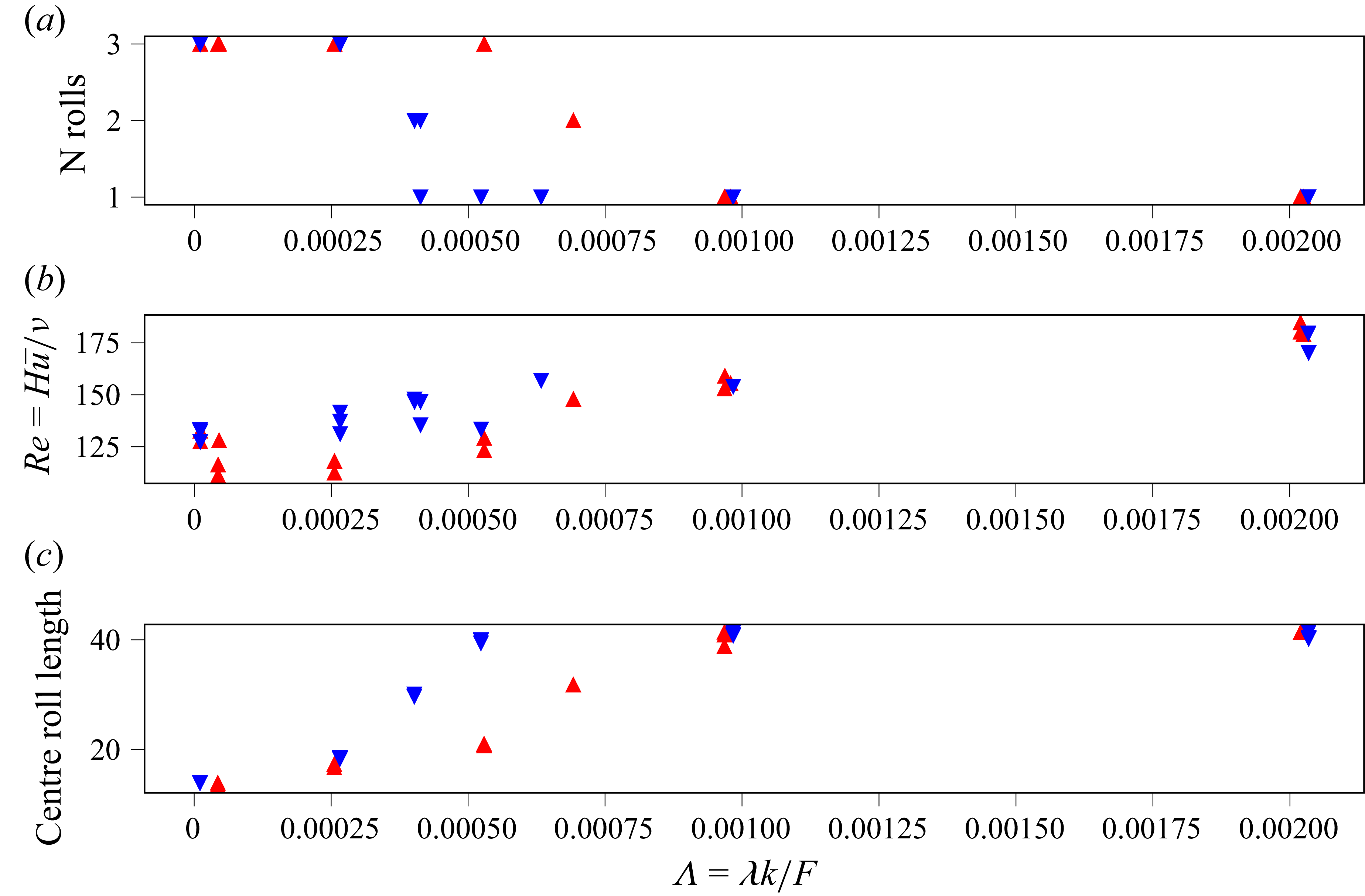
The analysis of the shadowgraph sequence can be carried out for several values of horizontal temperature gradient, at a given $ \textit{Ra}_F$
and
$ \textit{Ra}_F$
and $ \textit{Pr}$
, to determine the number of rolls as a function of
$ \textit{Pr}$
, to determine the number of rolls as a function of $\varLambda$
. The result is shown in figure 7(a). We observe an hysteretic transition at
$\varLambda$
. The result is shown in figure 7(a). We observe an hysteretic transition at $\varLambda _{{decr}} = {4\times 10^{-4}}$
when
$\varLambda _{{decr}} = {4\times 10^{-4}}$
when $\varLambda$
is decreasing, and at
$\varLambda$
is decreasing, and at $\varLambda _{\textit{incr}}={7\times 10^{-4}}$
when
$\varLambda _{\textit{incr}}={7\times 10^{-4}}$
when $\varLambda$
is increasing. These values are much smaller than those found in the two-dimensional DNS of Couston et al. (Reference Couston, Nandaha and Favier2022). Possible reasons for the difference might be the effects of three-dimensional dynamics, or the value of the Prandtl and Rayleigh numbers.
$\varLambda$
is increasing. These values are much smaller than those found in the two-dimensional DNS of Couston et al. (Reference Couston, Nandaha and Favier2022). Possible reasons for the difference might be the effects of three-dimensional dynamics, or the value of the Prandtl and Rayleigh numbers.
The maximum of the mean profile $\bar {u}(x, z_0)$
allows us to derive an estimate for the Reynolds number
$\bar {u}(x, z_0)$
allows us to derive an estimate for the Reynolds number
 \begin{align} Re = \frac {H\bar {u}}{\nu }, \end{align}
which is shown in figure 7-(b). In this set of experiments, we observe that the horizontal temperature gradient always yields an increase in velocity: in this case, we did not see a regime where the HC would oppose the vertical convection flow, which may have happened if the centre roll had been rotating clockwise. This could possibly be a mechanism for yet another hysteresis, but hence is not the cause of the currently observed one. The observed velocity is also hysteretic, with the velocity on the $\varLambda$
-decreasing branch higher than on the
$\varLambda$
-decreasing branch higher than on the $\varLambda$
-increasing branch, although the difference is not big (of order 10 %), and may be close to the experimental error.
$\varLambda$
-increasing branch, although the difference is not big (of order 10 %), and may be close to the experimental error.
The size of the centre roll can be estimated from the velocity profiles by finding the value of $x$
where the mean horizontal velocity is zero, i.e. where
$x$
where the mean horizontal velocity is zero, i.e. where $\bar {u}(x, z_0) = 0$
. The length of the roll goes from 14 cm (approximately a third of the cell width) at
$\bar {u}(x, z_0) = 0$
. The length of the roll goes from 14 cm (approximately a third of the cell width) at $\varLambda =0$
, to 41.5 cm (cell width) for
$\varLambda =0$
, to 41.5 cm (cell width) for $\varLambda \gg {4\times 10^{-4}}$
. As is shown in figure 7(c), and sketched in figure 6, the centre roll continuously grows when
$\varLambda \gg {4\times 10^{-4}}$
. As is shown in figure 7(c), and sketched in figure 6, the centre roll continuously grows when $\varLambda$
increases. At
$\varLambda$
increases. At $\varLambda ={5.3\times 10^{-4}}$
, its width is 20 cm but the third roll has not coalesced, so there are still 3 rolls. On the other hand, when
$\varLambda ={5.3\times 10^{-4}}$
, its width is 20 cm but the third roll has not coalesced, so there are still 3 rolls. On the other hand, when $\varLambda$
decreases from a large value, the roll size cannot decrease as long as a new roll has not appeared. We only observe a sharp decrease when a second roll has appeared. This suggests that there is a cost to change the number of rolls, and that this is the source of the hysteresis in this set of experiments. When
$\varLambda$
decreases from a large value, the roll size cannot decrease as long as a new roll has not appeared. We only observe a sharp decrease when a second roll has appeared. This suggests that there is a cost to change the number of rolls, and that this is the source of the hysteresis in this set of experiments. When $\varLambda$
is increasing, the number of rolls will remain equal to 3 but with decreasing size of the centre roll, and increasing size of the third roll. When
$\varLambda$
is increasing, the number of rolls will remain equal to 3 but with decreasing size of the centre roll, and increasing size of the third roll. When $\varLambda$
is decreasing,
$\varLambda$
is decreasing, $\varLambda$
has to decrease further, to
$\varLambda$
has to decrease further, to $4\times 10^{-4}$
, to break the unique roll into two asymmetric rolls (1/3 of the cell width for the roll on the left, 2/3 of the cell width for the roll on the right), and even further, to
$4\times 10^{-4}$
, to break the unique roll into two asymmetric rolls (1/3 of the cell width for the roll on the left, 2/3 of the cell width for the roll on the right), and even further, to $2.6\times 10^{-4}$
to break the rightmost roll and recover the three rolls structure.
$2.6\times 10^{-4}$
to break the rightmost roll and recover the three rolls structure.
The expected value of $\varLambda$
in SLs lies between
$\varLambda$
in SLs lies between $3\times 10^{-5}$
and
$3\times 10^{-5}$
and $3\times 10^{-4}$
(see table 1). The result of the DNS analysis was that
$3\times 10^{-4}$
(see table 1). The result of the DNS analysis was that $\varLambda \ll \varLambda _c \approx {10^-2}$
, therefore the lakes were expected to clearly be in the RBC regime. In this work, we find a threshold that is much closer to the
$\varLambda \ll \varLambda _c \approx {10^-2}$
, therefore the lakes were expected to clearly be in the RBC regime. In this work, we find a threshold that is much closer to the $\varLambda$
values in SLs. From our estimate of the critical value, we still expect that vertical RBC-type regime will be the main driving force, but some of these lakes, particularly those with larger
$\varLambda$
values in SLs. From our estimate of the critical value, we still expect that vertical RBC-type regime will be the main driving force, but some of these lakes, particularly those with larger $\varLambda$
may be in HC-type regime. Indeed, the values of
$\varLambda$
may be in HC-type regime. Indeed, the values of $\varLambda$
for the SLs are only estimates, and the critical value of
$\varLambda$
for the SLs are only estimates, and the critical value of $\varLambda$
may also differ at these higher
$\varLambda$
may also differ at these higher $ \textit{Pr}$
and
$ \textit{Pr}$
and $ \textit{Ra}_F$
values. We note that the nonlinearity of the equation of state for freshwater close to freezing may be a source of discrepancy between theoretical predictions such as drawn in this work, and flow structures in the field (Couston Reference Couston2021).
$ \textit{Ra}_F$
values. We note that the nonlinearity of the equation of state for freshwater close to freezing may be a source of discrepancy between theoretical predictions such as drawn in this work, and flow structures in the field (Couston Reference Couston2021).
4. Temperature stratification and internal gravity waves
Vertical temperature profiles, from sensors $p_1$
,
$p_1$
, $p_2$
,
$p_2$
, $p_3$
, respectively at
$p_3$
, respectively at $x_1={4.55}\,\textrm {cm}$
(blue circles),
$x_1={4.55}\,\textrm {cm}$
(blue circles), $x_2={20.7}\,\textrm {cm}$
(orange squares) and
$x_2={20.7}\,\textrm {cm}$
(orange squares) and $x_3={36.95}\,\textrm {cm}$
(green triangles), moving along the
$x_3={36.95}\,\textrm {cm}$
(green triangles), moving along the $z$
axis. (a) Rayleigh–Bénard-dominated regime (
$z$
axis. (a) Rayleigh–Bénard-dominated regime ( $\varLambda = {1.1\times 10^{-5}}$
), (b) at the threshold (
$\varLambda = {1.1\times 10^{-5}}$
), (b) at the threshold ( $\varLambda ={4.0\times 10^{-4}}$
), (c) HC-influenced regime with moderate horizontal gradient (
$\varLambda ={4.0\times 10^{-4}}$
), (c) HC-influenced regime with moderate horizontal gradient ( $\varLambda ={4.1\times 10^{-4}}$
) and (d) HC-influenced regime with large horizontal gradient (
$\varLambda ={4.1\times 10^{-4}}$
) and (d) HC-influenced regime with large horizontal gradient ( $\varLambda ={1.2\times 10^{-2}}$
).
$\varLambda ={1.2\times 10^{-2}}$
).
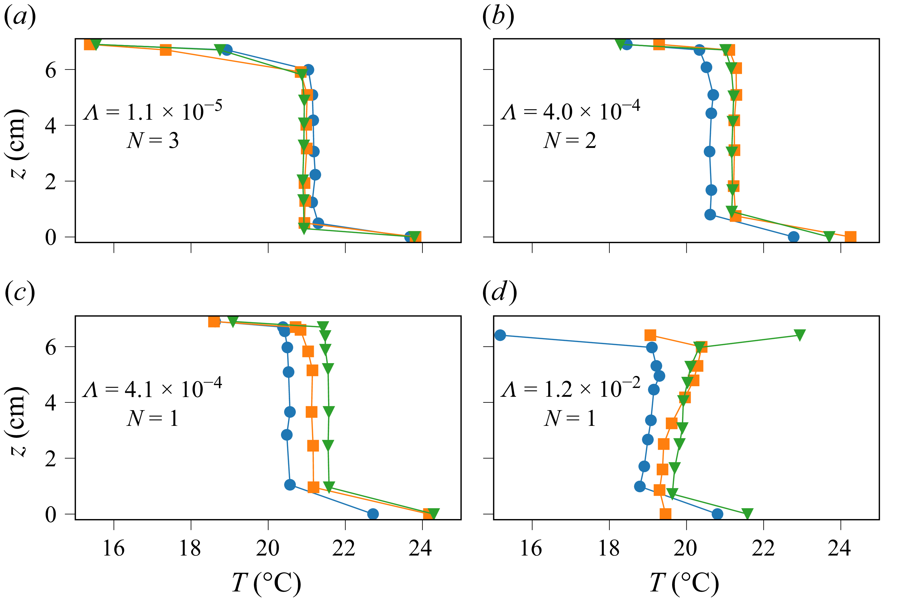
As shown in figure 8, each regime has a distinct signature in the temperature profiles.
At low $\varLambda$
, in the Rayleigh–Bénard-dominated regime, the mean temperature is homogeneous inside the bulk: the profiles from the three probes collapse, there is no dependency with either
$\varLambda$
, in the Rayleigh–Bénard-dominated regime, the mean temperature is homogeneous inside the bulk: the profiles from the three probes collapse, there is no dependency with either $x$
or
$x$
or $z$
. Note that the apparent asymmetry between the top and bottom parts of the profile stems from the fact that the probe can be moved inside the top plate, but cannot fully enter the boundary layer of the bottom plate. The closest it can be from the bottom plate is given by the size of the probe (4 mm).
$z$
. Note that the apparent asymmetry between the top and bottom parts of the profile stems from the fact that the probe can be moved inside the top plate, but cannot fully enter the boundary layer of the bottom plate. The closest it can be from the bottom plate is given by the size of the probe (4 mm).
At the threshold ( $N=2$
rolls), the temperature profiles obtained from probes 2 and 3, which are located inside the same roll, still collapse, but they differ from the profile obtained from probe 1. The temperature is still homogeneous within each roll, but the small roll on the left-hand side is colder than the large roll on the right-hand side.
$N=2$
rolls), the temperature profiles obtained from probes 2 and 3, which are located inside the same roll, still collapse, but they differ from the profile obtained from probe 1. The temperature is still homogeneous within each roll, but the small roll on the left-hand side is colder than the large roll on the right-hand side.
At larger $\varLambda$
, in the HC-influenced regime, the profiles no longer collapse, and a horizontal temperature gradient is visible inside the volume. For
$\varLambda$
, in the HC-influenced regime, the profiles no longer collapse, and a horizontal temperature gradient is visible inside the volume. For $\varLambda ={4.1\times 10^{-4}}$
, the vertical temperature gradient remains very small: even though the flow structure is heavily influenced by the horizontal temperature gradient, the mixing is still mostly similar to that of the Rayleigh–Bénard case. When
$\varLambda ={4.1\times 10^{-4}}$
, the vertical temperature gradient remains very small: even though the flow structure is heavily influenced by the horizontal temperature gradient, the mixing is still mostly similar to that of the Rayleigh–Bénard case. When $\varLambda$
is further increased, the temperature of the warmest side of the top plate gets close to that of the bottom plate, which results in an area within the cell where the fluid is stably stratified. In this regime, thermal plumes are no longer visible on the top right part of the cell. From the temperature profile at
$\varLambda$
is further increased, the temperature of the warmest side of the top plate gets close to that of the bottom plate, which results in an area within the cell where the fluid is stably stratified. In this regime, thermal plumes are no longer visible on the top right part of the cell. From the temperature profile at $\varLambda = {1.2\times 10^{-2}}$
, one can derive an estimate for the stable vertical temperature gradient,
$\varLambda = {1.2\times 10^{-2}}$
, one can derive an estimate for the stable vertical temperature gradient, $\delta T/\delta z \approx {0.29}\,\textrm {K}\,\textrm {cm}^{-1}$
, and therefore estimate the buoyancy frequency as (Belmonte et al. Reference Belmonte, Tilgner and Libchaber1995)
$\delta T/\delta z \approx {0.29}\,\textrm {K}\,\textrm {cm}^{-1}$
, and therefore estimate the buoyancy frequency as (Belmonte et al. Reference Belmonte, Tilgner and Libchaber1995)
 \begin{align} N = \sqrt {-\frac {g}{\rho }\frac {\mathrm{d}\rho }{\mathrm{d}z}} = \sqrt {g\alpha \frac {\delta T}{\delta z}}, \end{align}
of order 0.3 rad s−1 (or $N/(2\pi )$
of order 0.048 Hz).
$N/(2\pi )$
of order 0.048 Hz).
The possibility for the top plate to have one side warmer than the bottom plate is expected for large enough horizontal gradient $\lambda$
. Indeed, let us consider a simplified case where the top temperatures have three steps,
$\lambda$
. Indeed, let us consider a simplified case where the top temperatures have three steps, $T_1 \lt T_2 \lt T_3$
, with a linear relationship,
$T_1 \lt T_2 \lt T_3$
, with a linear relationship, $\lambda = (T_3 - T_1)/L$
and
$\lambda = (T_3 - T_1)/L$
and $T_2 = (T_1 + T_3)/2$
. The mean temperature drop between the top and bottom plate,
$T_2 = (T_1 + T_3)/2$
. The mean temperature drop between the top and bottom plate, $\Delta T$
, is linked to the RBC Nusselt number
$\Delta T$
, is linked to the RBC Nusselt number
 \begin{align} \textit{Nu} = \frac {FH}{k\Delta T}. \end{align}
For example, if the cell follows a $ \textit{Nu} = 0.06 Ra^{1/3}$
law, which is close to the experimental values of the literature in this range of Rayleigh numbers, as well as the local exponent in the Grossmann-Lohse model, then
$ \textit{Nu} = 0.06 Ra^{1/3}$
law, which is close to the experimental values of the literature in this range of Rayleigh numbers, as well as the local exponent in the Grossmann-Lohse model, then
 \begin{align} \Delta T = {\left ( \frac {\nu \kappa }{g\alpha }\right )}^{1/4}{\left ( \frac {F}{0.06 k} \right )}^{3/4}, \end{align}
and the condition for a temperature inversion is (with $T_2$
the mean temperature of the top plate)
$T_2$
the mean temperature of the top plate)
 \begin{align} T_3 \gt T_2 + \Delta T. \end{align}
With a linear gradient, $T_3 - T_2 = \lambda L/2$
, (4.4) becomes
$T_3 - T_2 = \lambda L/2$
, (4.4) becomes
 \begin{align} \lambda \gt \lambda _c = \frac {2}{L} {\left ( \frac {\nu \kappa }{g\alpha }\right )}^{1/4}{\left ( \frac {F}{0.06 k} \right )}^{3/4}. \end{align}
For a large enough horizontal temperature gradient, $\lambda$
, or small enough vertical heat flux,
$\lambda$
, or small enough vertical heat flux, $F$
, this condition can be met and there will be a temperature inversion. For the heat flux used in the present work (
$F$
, this condition can be met and there will be a temperature inversion. For the heat flux used in the present work ( $F = {0.232}\,{\,\textrm {W}\,\textrm {cm}^{-2}}$
) in deionised water at 20
$F = {0.232}\,{\,\textrm {W}\,\textrm {cm}^{-2}}$
) in deionised water at 20 $\,^\circ\textrm {C}$
, (4.5) yields
$\,^\circ\textrm {C}$
, (4.5) yields $\lambda _c = {570}\,{\,\textrm {mK}\,\textrm {cm}^{-1}}$
, which is a bit higher than our largest horizontal gradient (484 mK cm−1, see table 2), but close in order of magnitude. This very simple model is therefore consistent with the observed temperature profile, which is close to the temperature inversion threshold.
$\lambda _c = {570}\,{\,\textrm {mK}\,\textrm {cm}^{-1}}$
, which is a bit higher than our largest horizontal gradient (484 mK cm−1, see table 2), but close in order of magnitude. This very simple model is therefore consistent with the observed temperature profile, which is close to the temperature inversion threshold.
This configuration bears some similarity with systems where a stratified layer is located on top of a turbulent thermal convective layer, for example using water around its density maximum at 4 $\,^\circ\textrm {C}$
. In these systems, IGWs in the upper layer can be generated by the eddies of the turbulent convection in the bottom layer that impinge the upper stably stratified layer (Couston et al. Reference Couston, Lecoanet, Favier and Le Bars2018; Léard et al. Reference Léard, Favier, Le Gal and Le Bars2020). However, in these systems, the stratification is large, and the buoyancy frequency is much larger than the convective frequencies. The present case lies in the opposite regime, where the stratification is weak, and the buoyancy frequency smaller than the convective frequencies. In addition, the stratified medium is strongly sheared by the LSC. However, the top right region of the cell, which is devoid of thermal plumes at large values of
$\,^\circ\textrm {C}$
. In these systems, IGWs in the upper layer can be generated by the eddies of the turbulent convection in the bottom layer that impinge the upper stably stratified layer (Couston et al. Reference Couston, Lecoanet, Favier and Le Bars2018; Léard et al. Reference Léard, Favier, Le Gal and Le Bars2020). However, in these systems, the stratification is large, and the buoyancy frequency is much larger than the convective frequencies. The present case lies in the opposite regime, where the stratification is weak, and the buoyancy frequency smaller than the convective frequencies. In addition, the stratified medium is strongly sheared by the LSC. However, the top right region of the cell, which is devoid of thermal plumes at large values of $\varLambda$
, show some low-frequency signal. In the following, we investigate this signal, and show evidence supporting the presence of IGWs. Note that the existence of IGWs, and their interplay with the thermal flow, is well known in the case of differentially heated cavities, where an area of stably stratified fluid settles (Patterson & Imberger Reference Patterson and Imberger1980; Chorin, Moreau & Saury Reference Chorin, Moreau and Saury2021; Le Quéré Reference Le Quéré2022).
$\varLambda$
, show some low-frequency signal. In the following, we investigate this signal, and show evidence supporting the presence of IGWs. Note that the existence of IGWs, and their interplay with the thermal flow, is well known in the case of differentially heated cavities, where an area of stably stratified fluid settles (Patterson & Imberger Reference Patterson and Imberger1980; Chorin, Moreau & Saury Reference Chorin, Moreau and Saury2021; Le Quéré Reference Le Quéré2022).
The most common method for the visualisation of IGWs is synthetic schlieren (Dalziel, Hugues & Sutherland Reference Dalziel, Hugues and Sutherland2000), which grants access to the density gradients. This has been used extensively in salt water experiments, for example to evidence the destabilisation of internal waves into secondary lower-frequency waves via a triadic resonant instability (Bourget et al. Reference Bourget, Dauxois, Joubaud and Odier2013), and the destruction of background stratification in attractors through enhanced wave-induced mixing at hotspots (Scolan, Ermanyuk & Dauxois Reference Scolan, Ermanyuk and Dauxois2013). In this work, we use shadowgraph instead of synthetic schlieren, because it is better suited to the visualisation of thermal plumes. Indeed, thermal plumes produce strong and localised density gradients at their boundaries, while the background density in the bulk of turbulent thermal convection show much smaller fluctuations. While synthetic schlieren can be used also in this situation, and has been shown to provide useful insights (Salort et al. Reference Salort, Liot, Rusaouen, Seychelles, Tisserand, Creyssels, Castaing and Chillà2014), it requires a dense dot pattern and high camera resolution, or zooming on a smaller area of the convection cell.
The shadowgraph images, $I(x, z, t)$
, are determined by the second derivative of the refractive index (Settles Reference Settles2001), given by (2.2). As discussed in Belkadi et al. (Reference Belkadi, Guislain, Sergent, Podvin, Chillà and Salort2020), in the limit of the small temperature fluctuations within the Boussinesq conditions, the refractive index variations are proportional to the density variations, the density variations are proportional to the temperature variations and the shadowgraph image can be written, at leading order,
$I(x, z, t)$
, are determined by the second derivative of the refractive index (Settles Reference Settles2001), given by (2.2). As discussed in Belkadi et al. (Reference Belkadi, Guislain, Sergent, Podvin, Chillà and Salort2020), in the limit of the small temperature fluctuations within the Boussinesq conditions, the refractive index variations are proportional to the density variations, the density variations are proportional to the temperature variations and the shadowgraph image can be written, at leading order,
 \begin{align} \frac {I(x, z, t)}{I_0} \propto \int _0^D\left (\frac {\partial ^2T}{\partial x^2} + \frac {\partial ^2T}{\partial z^2}\right )\mathrm{d}y. \end{align}
A monochromatic IGW, characterised by a wave vector $\boldsymbol{k}$
and a pulsation
$\boldsymbol{k}$
and a pulsation $\omega$
, produces a density perturbation
$\omega$
, produces a density perturbation $\delta \rho \sim \rho _0e^{i(\boldsymbol{k}\boldsymbol{\cdot }\boldsymbol{r} - \omega t)}$
. The second derivative of (4.6) will conserve this spatial structure, and therefore the perturbation
$\delta \rho \sim \rho _0e^{i(\boldsymbol{k}\boldsymbol{\cdot }\boldsymbol{r} - \omega t)}$
. The second derivative of (4.6) will conserve this spatial structure, and therefore the perturbation $\delta \rho$
should be directly visible in the shadowgraph image.
$\delta \rho$
should be directly visible in the shadowgraph image.
Temporal energy spectra from the shadowgraph signal, spatially averaged in the top right corner (blue lines), or in the bottom left corner (red lines). (a) Spectra obtained in the case of a smaller horizontal temperature gradient ( $\varLambda = {9.7\times 10^{-4}}$
, still large enough to be in HC-influenced regime, but top right corner has thermal plumes); (b) spectra obtained in the case of a large horizontal temperature gradient (
$\varLambda = {9.7\times 10^{-4}}$
, still large enough to be in HC-influenced regime, but top right corner has thermal plumes); (b) spectra obtained in the case of a large horizontal temperature gradient ( $\varLambda = {1.2\times 10^{-2}}$
, top right corner devoid of thermal plumes). The black lines are visual indicator of a
$\varLambda = {1.2\times 10^{-2}}$
, top right corner devoid of thermal plumes). The black lines are visual indicator of a $f^{-0.7}$
scaling law.
$f^{-0.7}$
scaling law.

The temporal dynamics is determined experimentally by computing the Fourier transform of the shadowgraph image, $I(x, z, t)$
, along the time axis,
$I(x, z, t)$
, along the time axis, $\hat {I}(x, z, \omega )$
, and then spatially averaging its modulus squared, i.e.
$\hat {I}(x, z, \omega )$
, and then spatially averaging its modulus squared, i.e.
 \begin{align} E(\omega ) = \big \langle | \hat {I}(x, z, \omega ) |^2 \big \rangle _{x, z}. \end{align}
The energy spectrum, $E(\omega )$
, obtained by performing the spatial average in the top right region (plume free at large
$E(\omega )$
, obtained by performing the spatial average in the top right region (plume free at large $\varLambda$
) is compared with the energy spectrum obtained by performing the spatial average in the symmetric bottom left region (figure 9).
$\varLambda$
) is compared with the energy spectrum obtained by performing the spatial average in the symmetric bottom left region (figure 9).
At moderate values of $\varLambda$
(figure 9
a), the spectra are quite similar in the top-right and bottom-left regions, which shows that the temperature fluctuations have similar statistics near the top and near the bottom plate. While the horizontal temperature gradient is strong enough to change the flow structure and introduce a horizontal temperature gradient in the bulk (breaking the left–right symmetry), it is not strong enough to break the bottom–top symmetry. The spectrum is also nearly white, or slowly decreasing, in a wide range of frequencies below
$\varLambda$
(figure 9
a), the spectra are quite similar in the top-right and bottom-left regions, which shows that the temperature fluctuations have similar statistics near the top and near the bottom plate. While the horizontal temperature gradient is strong enough to change the flow structure and introduce a horizontal temperature gradient in the bulk (breaking the left–right symmetry), it is not strong enough to break the bottom–top symmetry. The spectrum is also nearly white, or slowly decreasing, in a wide range of frequencies below $f_c \approx {0.2}\,\textrm {Hz}$
. The length scale associated with this frequency is
$f_c \approx {0.2}\,\textrm {Hz}$
. The length scale associated with this frequency is $\bar {u} / f_c \approx {1}\,\textrm {cm}$
, which is close to the typical distance between thermal plumes (see figure 4). For
$\bar {u} / f_c \approx {1}\,\textrm {cm}$
, which is close to the typical distance between thermal plumes (see figure 4). For $f \gt f_c$
, there is a short range, where the fluctuations decrease like
$f \gt f_c$
, there is a short range, where the fluctuations decrease like $f^{-\alpha }$
, with
$f^{-\alpha }$
, with $\alpha \approx 0.7$
.
$\alpha \approx 0.7$
.
The value of this exponent is phenomenological, and cannot be directly compared with the literature. Indeed, spatial derivatives of the temperature have a smaller scaling exponent than the temperature fluctuations. In particular Sreenivasan, Bershadskii & Niemela (Reference Sreenivasan, Bershadskii and Niemela2005) found $f^{-1}$
scaling for the fluctuations of the temperature gradients. In the case of fluctuations of shadowgraph (second derivative of temperature, integrated over the depth of the cell), away from the centre, there is no prediction for
$f^{-1}$
scaling for the fluctuations of the temperature gradients. In the case of fluctuations of shadowgraph (second derivative of temperature, integrated over the depth of the cell), away from the centre, there is no prediction for $\alpha$
, and the phenomenological value
$\alpha$
, and the phenomenological value $\alpha =0.7$
would surely depend on where it is computed inside the cell.
$\alpha =0.7$
would surely depend on where it is computed inside the cell.
At large values of $\varLambda$
(figure 9
b), the spectrum significantly differs in the top-right region compared with the bottom-left region where the dynamics is still dominated by plumes. There is much less energy in the range
$\varLambda$
(figure 9
b), the spectrum significantly differs in the top-right region compared with the bottom-left region where the dynamics is still dominated by plumes. There is much less energy in the range $f \gt f_c = {0.2}\,\textrm {Hz}$
, and no inertial range, which shows that there is no turbulent convection, and no thermal plumes, in this region. In the bottom-left region, a spectrum close to that of turbulent convection is recovered. Additionally, the top-right region show a number of peaks at lower frequencies: one peak at
$f \gt f_c = {0.2}\,\textrm {Hz}$
, and no inertial range, which shows that there is no turbulent convection, and no thermal plumes, in this region. In the bottom-left region, a spectrum close to that of turbulent convection is recovered. Additionally, the top-right region show a number of peaks at lower frequencies: one peak at $f_0 \approx {0.014}\,\textrm {Hz}$
, as well as its harmonic
$f_0 \approx {0.014}\,\textrm {Hz}$
, as well as its harmonic $2f_0 \approx {0.028}\,\textrm {Hz}$
. These may be waves, excited by the slower oscillations of the LSC, similar to those observed by Belmonte et al. (Reference Belmonte, Tilgner and Libchaber1995) in the case of side-heated convection. Indeed, the LSC in RBC exhibits slow motions on time scales much larger than that of the plumes: torsional oscillations (Funfschilling, Brown & Ahlers Reference Funfschilling, Brown and Ahlers2008), oscillation of the direction of the mean flow (Resagk et al. Reference Resagk, du Puits, Thess, Dolzhansky, Grossmann, Araujo and Lohse2006) or sloshing motion of the convection roll (Liot et al. Reference Liot, Gay, Salort, Bourgoin and Chillà2016). These slow motions of the LSC may play a similar roll in our model system as the tidal forcing in natural settings. The actual frequencies that are selected in the system will be those that match the dispersion relation for the internal waves with admissible wavenumbers.
$2f_0 \approx {0.028}\,\textrm {Hz}$
. These may be waves, excited by the slower oscillations of the LSC, similar to those observed by Belmonte et al. (Reference Belmonte, Tilgner and Libchaber1995) in the case of side-heated convection. Indeed, the LSC in RBC exhibits slow motions on time scales much larger than that of the plumes: torsional oscillations (Funfschilling, Brown & Ahlers Reference Funfschilling, Brown and Ahlers2008), oscillation of the direction of the mean flow (Resagk et al. Reference Resagk, du Puits, Thess, Dolzhansky, Grossmann, Araujo and Lohse2006) or sloshing motion of the convection roll (Liot et al. Reference Liot, Gay, Salort, Bourgoin and Chillà2016). These slow motions of the LSC may play a similar roll in our model system as the tidal forcing in natural settings. The actual frequencies that are selected in the system will be those that match the dispersion relation for the internal waves with admissible wavenumbers.
The spectrum also shows secondary peaks, which may stem from the destabilisation of these internal waves forced by the large-scale convective flow. The mechanism may be triadic resonance instability (Boury et al. Reference Boury, Maurer, Joubaud, Peacock and Odier2023), where a wave of pulsation $\omega _0$
gives birth to two secondary waves with lower pulsations
$\omega _0$
gives birth to two secondary waves with lower pulsations $\omega _1$
and
$\omega _1$
and $\omega _2$
, such that
$\omega _2$
, such that
 \begin{align} \omega _0 = \omega _1 + \omega _2. \end{align}
In such a case, the two peaks at $f_{s1} = {6.2\times 10^{-3}}\,\textrm {Hz}$
and
$f_{s1} = {6.2\times 10^{-3}}\,\textrm {Hz}$
and $f_{s2} = {7.8\times 10^{-3}}\,\textrm {Hz}$
are signatures of secondary waves generated by the main wave at
$f_{s2} = {7.8\times 10^{-3}}\,\textrm {Hz}$
are signatures of secondary waves generated by the main wave at $f_0$
, and the two peaks at
$f_0$
, and the two peaks at $f_{s3} = {1.2\times 10^{-2}}\,\textrm {Hz}$
and
$f_{s3} = {1.2\times 10^{-2}}\,\textrm {Hz}$
and $f_{s4} = {1.6\times 10^{-2}}\,\textrm {Hz}$
are signatures of secondary waves generated by the main wave at
$f_{s4} = {1.6\times 10^{-2}}\,\textrm {Hz}$
are signatures of secondary waves generated by the main wave at $2f_0$
. Interestingly, the peaks are also visible on the bottom left corner, although they are much weaker, which suggests that the density perturbations are advected by the mean flow, and have not yet dissipated when they reach the opposite side of the cell.
$2f_0$
. Interestingly, the peaks are also visible on the bottom left corner, although they are much weaker, which suggests that the density perturbations are advected by the mean flow, and have not yet dissipated when they reach the opposite side of the cell.
(a) Example of bandpass filtered shadowgraph field, around the frequency $f_{s,3}$
. The wavelength and angle of the wave near
$f_{s,3}$
. The wavelength and angle of the wave near $x = {29.5}\,\textrm {cm}$
is annotated as
$x = {29.5}\,\textrm {cm}$
is annotated as $\lambda _w$
and
$\lambda _w$
and $\theta$
. (b) Dispersion relation for several frequencies, at the same location (
$\theta$
. (b) Dispersion relation for several frequencies, at the same location ( $x = {29.5}\,\textrm {cm}$
). The slope of the solid line is
$x = {29.5}\,\textrm {cm}$
). The slope of the solid line is $2\pi \bar {u}(z_0 = {6}\,\textrm {cm})$
and the ordinate at the origin is
$2\pi \bar {u}(z_0 = {6}\,\textrm {cm})$
and the ordinate at the origin is $-N$
(see (4.12)).
$-N$
(see (4.12)).

To characterise the spatial structure of these waves, we apply a fourth-order Butterworth bandpass filter along the time axis of the shadowgraph images $I(x, y, t)$
. As shown in figure 10, the angle
$I(x, y, t)$
. As shown in figure 10, the angle $\theta$
of the wave is quite small (less than 3
$\theta$
of the wave is quite small (less than 3 $^\circ$
), much smaller than what would be expected by the usual dispersion relation in a quiescent fluid
$^\circ$
), much smaller than what would be expected by the usual dispersion relation in a quiescent fluid
 \begin{align} \omega = N\sin \theta , \end{align}
which gives $\theta = {14}{^\circ }$
for
$\theta = {14}{^\circ }$
for $N/(2\pi ) = {0.048}\,\textrm {Hz}$
and
$N/(2\pi ) = {0.048}\,\textrm {Hz}$
and $f_{s3} = {1.2\times 10^{-2}}\,\textrm {Hz}$
. This is due to the strong horizontal velocity, which stretches the internal waves in the
$f_{s3} = {1.2\times 10^{-2}}\,\textrm {Hz}$
. This is due to the strong horizontal velocity, which stretches the internal waves in the $x$
direction. Indeed, the importance of the mean horizontal velocity can be assessed by the Richardson number,
$x$
direction. Indeed, the importance of the mean horizontal velocity can be assessed by the Richardson number, $Ri$
,
$Ri$
,
 \begin{align} Ri = \frac {N^2}{{(\delta U/\delta z)}^2}, \end{align}
which is of order $Ri \sim 20 \gt {1}/{4}$
in our system. In this regime, the dispersion relation of IGWs is the Doppler-shifted dispersion relation, given by (Booker & Bretherton Reference Booker and Bretherton1967; Howland, Taylor & Caulfield Reference Howland, Taylor and Caulfield2021)
$Ri \sim 20 \gt {1}/{4}$
in our system. In this regime, the dispersion relation of IGWs is the Doppler-shifted dispersion relation, given by (Booker & Bretherton Reference Booker and Bretherton1967; Howland, Taylor & Caulfield Reference Howland, Taylor and Caulfield2021)
 \begin{align} \omega (k_x, k_z, z) = \bar {u}(z)k_x + \frac {{k_x}N}{\sqrt {k_x^2 + k_z^2}}, \end{align}
which we can write as
 \begin{align} \omega = \left ( \frac {2\pi \bar {u}}{\lambda _w} \pm N\right )\sin \theta , \end{align}
where $\lambda _w$
is the wavelength of the wave,
$\lambda _w$
is the wavelength of the wave, $\bar {u}$
is the outer horizontal flow velocity,
$\bar {u}$
is the outer horizontal flow velocity, $N$
is the buoyancy pulsation,
$N$
is the buoyancy pulsation, $\omega$
is the pulsation of the wave and
$\omega$
is the pulsation of the wave and $\sin \theta$
is the angle between the wavevector of the wave and the vertical.
$\sin \theta$
is the angle between the wavevector of the wave and the vertical.
To verify the dispersion relation, we plot $\omega /\sin \theta$
versus
$\omega /\sin \theta$
versus $1/\lambda _w$
in figure 10(b), for the main modes detected in the spectrum (figure 9
b), and we find that the data are fairly compatible with (4.12). These values of (
$1/\lambda _w$
in figure 10(b), for the main modes detected in the spectrum (figure 9
b), and we find that the data are fairly compatible with (4.12). These values of ( $\lambda _w$
,
$\lambda _w$
, $\omega$
) have been obtained from the same shadowgraph sequence, at
$\omega$
) have been obtained from the same shadowgraph sequence, at $\varLambda ={1.2\times 10^{-2}}$
, bandpass filtered at several frequencies
$\varLambda ={1.2\times 10^{-2}}$
, bandpass filtered at several frequencies $\omega /(2\pi )$
. The fitting parameters yield
$\omega /(2\pi )$
. The fitting parameters yield $\bar {u} = {0.13}\,\textrm {cm}\,\textrm {s}^{-1}$
and
$\bar {u} = {0.13}\,\textrm {cm}\,\textrm {s}^{-1}$
and $N = {0.37}\,\textrm {rad}\,\textrm {s}^{-1}$
(corresponding to a vertical temperature gradient 0.68 K cm−1, using (4.1)). Although we do not have the resolution in either velocity or temperature profiles in this region to directly compare with these values, they are not unreasonable, and are fairly compatible with the temperature profile shown in figure 8. While the maximum horizontal velocity from figure 6 near the bottom plate is of order 0.2 cm s−1, the velocity closer to the plate might be lower. Therefore, the peaks observed in the spectrum are waves, and are compatible, within experimental accuracy, with IGWs with a background horizontal velocity.
$N = {0.37}\,\textrm {rad}\,\textrm {s}^{-1}$
(corresponding to a vertical temperature gradient 0.68 K cm−1, using (4.1)). Although we do not have the resolution in either velocity or temperature profiles in this region to directly compare with these values, they are not unreasonable, and are fairly compatible with the temperature profile shown in figure 8. While the maximum horizontal velocity from figure 6 near the bottom plate is of order 0.2 cm s−1, the velocity closer to the plate might be lower. Therefore, the peaks observed in the spectrum are waves, and are compatible, within experimental accuracy, with IGWs with a background horizontal velocity.
(a) Zoom on the bandpass filtered shadowgraph field, around the frequency $f_{s,3}$
. The green dashed lines show where the space–time diagrams are obtained from. (b) Space–time diagram along the horizontal line at
$f_{s,3}$
. The green dashed lines show where the space–time diagrams are obtained from. (b) Space–time diagram along the horizontal line at $z={6.0}\,\textrm {cm}$
. (c) Space–time diagram along the vertical line at
$z={6.0}\,\textrm {cm}$
. (c) Space–time diagram along the vertical line at $x={30.5\,\textrm {cm}}$
. The green dashed line has a slope
$x={30.5\,\textrm {cm}}$
. The green dashed line has a slope ${6.7\times 10^{-3}}\,\textrm {cm}\,\textrm {s}^{-1}$
.
${6.7\times 10^{-3}}\,\textrm {cm}\,\textrm {s}^{-1}$
.

The phase speed of the internal waves can be measured from a space–time diagram of the bandpass-filtered shadowgraph, as shown in figure 11 for $f_{s,3}$
. The expected phase speed can be derived from the dispersion relation (4.12)
$f_{s,3}$
. The expected phase speed can be derived from the dispersion relation (4.12)
 \begin{align} \boldsymbol{v}_{\phi } = \left ( \bar {u} \pm \frac {N\lambda _w}{2\pi }\right )\sin {\theta }\left ( \sin {\theta }\boldsymbol{e}_x + \cos {\theta }\boldsymbol{e}_z\right ), \end{align}
where $\boldsymbol{e}_x, \boldsymbol{e}_z$
are the horizontal and vertical base vectors. Because
$\boldsymbol{e}_x, \boldsymbol{e}_z$
are the horizontal and vertical base vectors. Because $\theta$
is small (
$\theta$
is small ( $\sin {\theta } \approx {4.3\times 10^{-2}}$
), the horizontal velocity is vanishingly small (
$\sin {\theta } \approx {4.3\times 10^{-2}}$
), the horizontal velocity is vanishingly small ( ${3.2\times 10^{-4}}\,\textrm {cm}\,\textrm {s}^{-1}$
from (4.13)), but the vertical velocity, although small (
${3.2\times 10^{-4}}\,\textrm {cm}\,\textrm {s}^{-1}$
from (4.13)), but the vertical velocity, although small ( ${7.5\times 10^{-3}}\,\textrm {cm}\,\textrm {s}^{-1}$
from (4.13)), can be compared with the shadowgraph recording. The green dashed slope in figure 11(c) is
${7.5\times 10^{-3}}\,\textrm {cm}\,\textrm {s}^{-1}$
from (4.13)), can be compared with the shadowgraph recording. The green dashed slope in figure 11(c) is ${6.7\times 10^{-3}}\,\textrm {cm}\,\textrm {s}^{-1}$
, which is fairly compatible with the expected value.
${6.7\times 10^{-3}}\,\textrm {cm}\,\textrm {s}^{-1}$
, which is fairly compatible with the expected value.
The group speed of the waves
 \begin{align} \boldsymbol{v}_g = \bar {u}\boldsymbol{e}_x \pm \frac {N\lambda _w\cos {\theta }}{2\pi }\left ( \cos {\theta }\boldsymbol{e}_x + \sin {\theta }\boldsymbol{e}_z \right ), \end{align}
is expected to be mostly horizontal, but cannot be directly measured in this case.
5. Conclusion
In this paper, we presented an experimental realisation of a simple model of SLs. We find that the dynamics is varied and identify different regimes: pure RBC convection, mixed RBC/HC convection where the convective rolls eventually merge into a unique large roll and the HC regime, where thermal convection impinges on a stratified layer and triggers IGWs, which are then advected by the LSC.
While the experimental investigation of this model system improves our understanding of the physics of natural systems such as SLs on Earth, or icy moons in the solar system (Gastine & Favier Reference Gastine and Favier2025), it can also be seen as another way to introduce perturbations in turbulent thermal convection, and therefore ascertain the robustness of theoretical predictions to changes in flow conditions, such as the change of LSC structure in the mixed RBC/HC regime.
Acknowledgements
The authors warmly thank M. Moulin for the design and construction of the apparatus on particularly short notice, which helped maintain the schedule for the Valentine internship. This work benefited from computing resources provided by the CBPsmn (PSMN, Pôle Scientifique de Modélisation Numérique) of ENS de Lyon. The platform operates the SIDUS solution developed by E. Quemener and Corvellec (2013).
The authors also thank several colleagues from the Laboratoire de Physique, including J. Deleuze, C. Jacob, S. Joubaud, and P. Odier, as well as H. Scolan from LMFA laboratory, for valuable discussions, particularly regarding IGWs. Additional thanks are extended to A. Sergent and N. Carbonneau from LISN laboratory for their inputs. The authors are also grateful to the students working on the next iteration of the experiment, V. Chanut and C. Bret.
Funding
This work received financial support from the LABEX Lyon Institute of Origins (ANR-10-LABX-0066) under the Plan France 2030 program of the French government, operated by the National Research Agency (ANR). Y.-Z. Bu acknowledges support from the China Scholarship Council (CSC) through a PhD scholarship. Additional funding for Y.-Z. Bu was provided by the Graduate Initiative PACE (SFRI Graduate+).
Declaration of interests
The authors report no conflicts of interest.




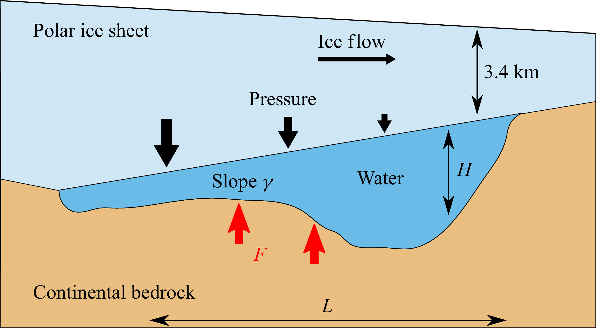


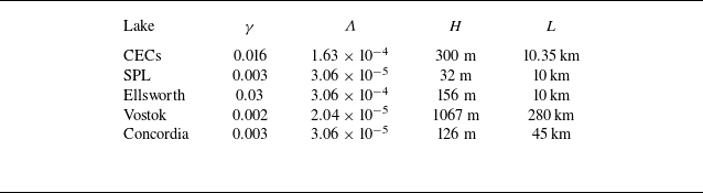


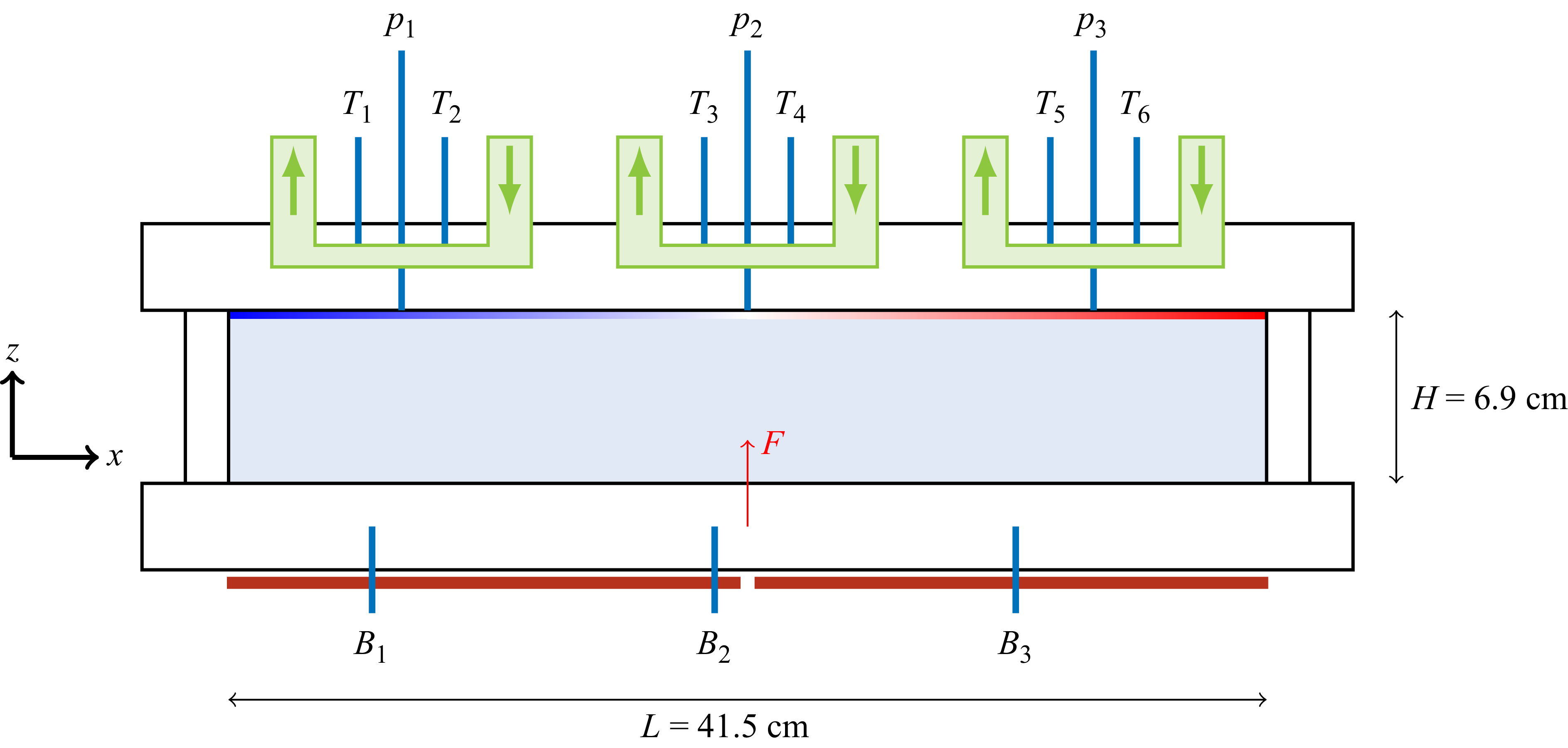


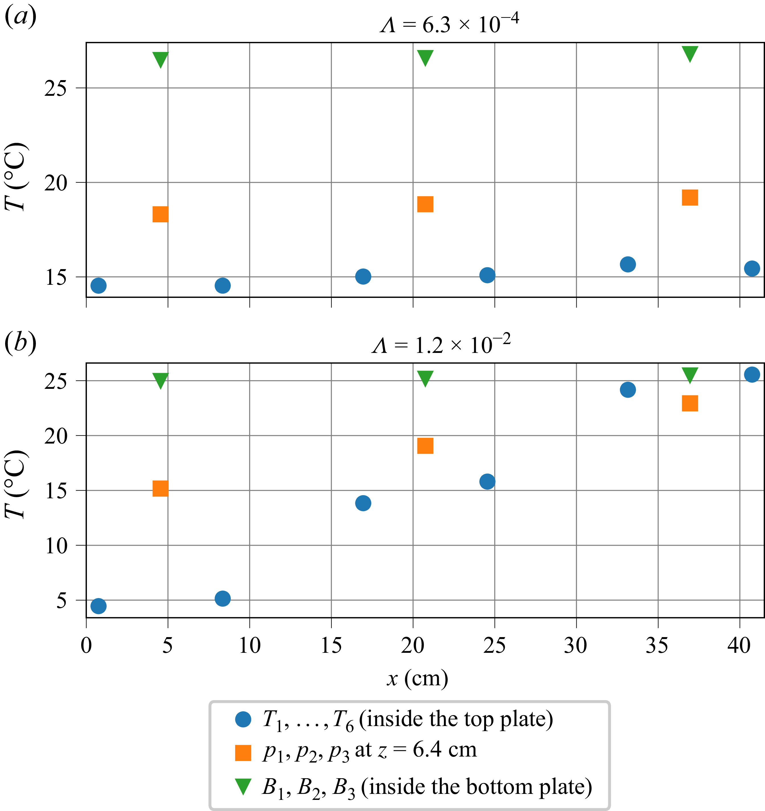
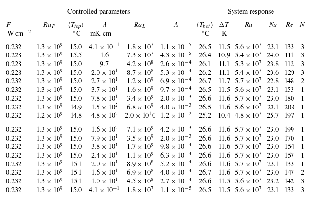


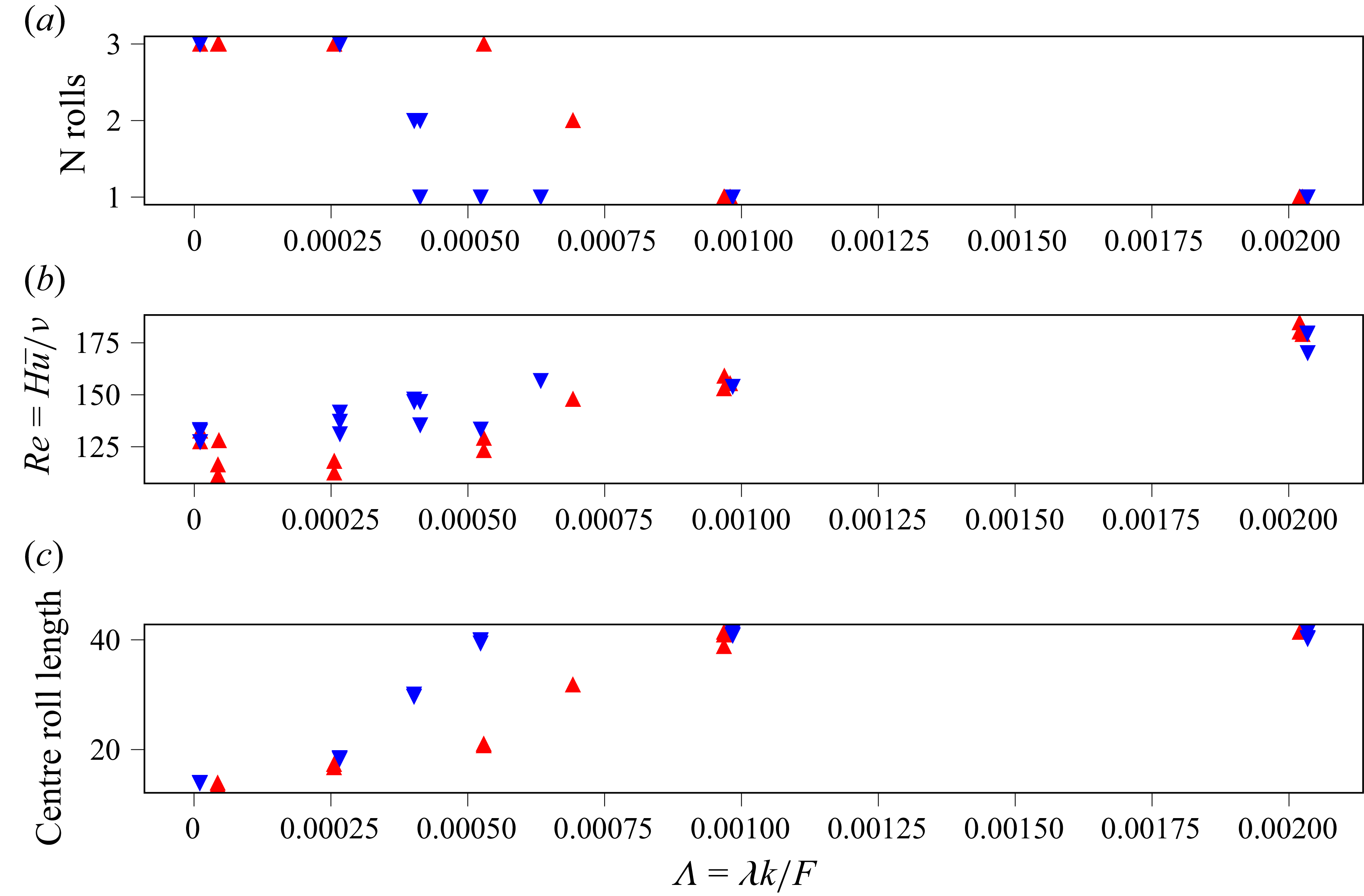


 Open access

