


1. Introduction
Let $K_d \subset \mathbb{R}^d$
be a d-dimensional convex body and let
$K_d \subset \mathbb{R}^d$
be a d-dimensional convex body and let $\mathbf{X},\mathbf{Y},\mathbf{Z}\sim\mathsf{Unif}(K_d)$
be three random points selected from the interior of
$\mathbf{X},\mathbf{Y},\mathbf{Z}\sim\mathsf{Unif}(K_d)$
be three random points selected from the interior of $K_d$
uniformly and independently. The objective of this paper is to study the obtusity probability in
$K_d$
uniformly and independently. The objective of this paper is to study the obtusity probability in $K_d$
. That is, the probability
$K_d$
. That is, the probability $\eta(K_d)$
that the random triangle
$\eta(K_d)$
that the random triangle $\mathbf{X}\mathbf{Y}\mathbf{Z}$
is obtuse.
$\mathbf{X}\mathbf{Y}\mathbf{Z}$
is obtuse.
In two dimensions, there are several known results. The obtusity probability was first solved in a disk $\mathbb{B}_2$
in [Reference Woolhouse18] as a corollary to the Silvester problem. It reads
$\mathbb{B}_2$
in [Reference Woolhouse18] as a corollary to the Silvester problem. It reads
 \begin{equation*}\eta(\mathbb{B}_2) = \frac{9}{8} - \frac{4}{\pi^2}\approx 0.7197.\end{equation*}
Later, Langford [Reference Langford11] found $\eta(K_2)$
for
$\eta(K_2)$
for $K_2$
being a general rectangle. The special case of
$K_2$
being a general rectangle. The special case of $\eta(C_2)$
, where
$\eta(C_2)$
, where $C_2$
is the unit square, yields
$C_2$
is the unit square, yields
 \begin{equation*} \eta(C_2) = \frac{97}{150}+\frac{\pi}{40} \approx 0.7252.\end{equation*}
It is a simple exercise to deduce $\eta(T_2)$
, where
$\eta(T_2)$
, where $T_2$
is a general triangle. This is, however, not the content of this paper. The general result is not very illuminating either. For example, we have
$T_2$
is a general triangle. This is, however, not the content of this paper. The general result is not very illuminating either. For example, we have
 \begin{equation*} \eta(T_2^*) = \frac{25}{4}+\frac{\pi }{12 \sqrt{3}}+\frac{393}{10} \ln\frac{\sqrt{3}}{2} \approx 0.7482,\end{equation*}
where $T_2^*$
denotes the equilateral triangle (minimum value among all triangles).
$T_2^*$
denotes the equilateral triangle (minimum value among all triangles).
In higher dimensions, there is a famous result by Hall [Reference Hall10] and Buchta and Müller [Reference Buchta and Müller5]. They were able to deduce $\eta(\mathbb{B}_d)$
explicitly, where
$\eta(\mathbb{B}_d)$
explicitly, where $\mathbb{B}_d$
is the d-ball, for any value of
$\mathbb{B}_d$
is the d-ball, for any value of $d\geq 2$
. For example, they obtained
$d\geq 2$
. For example, they obtained
 \begin{equation*} \eta(\mathbb{B}_3) = \frac{37}{70} \approx 0.5286.\end{equation*}
Apart from the d-ball, $\eta(K_d)$
is not known for any
$\eta(K_d)$
is not known for any $K_d$
with
$K_d$
with $d \geq 3$
. The only exception, as shown in this paper, is the obtusity probability in the unit cube
$d \geq 3$
. The only exception, as shown in this paper, is the obtusity probability in the unit cube $C_3$
. The problem was suggested by Finch in his monographs Mathematical Constants Volume I [Reference Finch8, p. 480] and Volume II [Reference Finch9, p. 693]. Weisstein [Reference Weisstein17] obtained a numerical estimate
$C_3$
. The problem was suggested by Finch in his monographs Mathematical Constants Volume I [Reference Finch8, p. 480] and Volume II [Reference Finch9, p. 693]. Weisstein [Reference Weisstein17] obtained a numerical estimate $\eta(C_3)\approx 0.5425$
. We obtained
$\eta(C_3)\approx 0.5425$
. We obtained
 \begin{align*}\eta(C_3) &= \frac{323\,338}{385\,875}-\frac{13G}{35}+\frac{4859 \pi }{62\,720}-\frac{73 \pi }{1680 \sqrt{2}}-\frac{\pi ^2}{105}+\frac{3\pi \ln 2}{224}-\frac{3\pi \ln(1+\sqrt{2})}{224}\\ &\approx 0.542\,659\,281\,4,\end{align*}
where $G= \sum_{n=0}^\infty\frac{(-1)^n}{(2n+1)^2}\approx 0.915\,965\,594\,1$
is Catalan’s constant. This result is new as far as we know. Note that one can easily recreate Weisstein’s numerical estimate of
$G= \sum_{n=0}^\infty\frac{(-1)^n}{(2n+1)^2}\approx 0.915\,965\,594\,1$
is Catalan’s constant. This result is new as far as we know. Note that one can easily recreate Weisstein’s numerical estimate of $\eta(C_3)$
(see Appendix A for a Monte Carlo implementation in Mathematica).
$\eta(C_3)$
(see Appendix A for a Monte Carlo implementation in Mathematica).
A related question is finding the random triangle’s largest internal angle distribution, from which the obtusity probability can also be deduced. Eisenberg and Sullivan [Reference Eisenberg and Sullivan6] found this distribution in the unit disk.
2. Preliminaries
2.1. Langford and related distributions
Let $U,U',U''\sim \mathsf{Unif}(0,1)$
(independent). We define four random variables
$U,U',U''\sim \mathsf{Unif}(0,1)$
(independent). We define four random variables
 \begin{equation*} \Lambda = (U'-U)(U''-U),\quad \Sigma = (U-U')U,\quad \Xi = UU',\quad \Omega = U(1-U).\end{equation*}
The equalities between $\Lambda,\Sigma,\Xi,\Omega$
with U,U’,U” have to be interpreted only in terms of distributions. We say that
$\Lambda,\Sigma,\Xi,\Omega$
with U,U’,U” have to be interpreted only in terms of distributions. We say that $\Lambda$
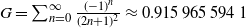
follows the Langford distribution [Reference Langford11]. We refer to those four variables as our paper’s auxiliary random variables. Their probability density functions (PDFs) and the cumulative density functions (CDFs) are given in Table 1. Trivially, the PDF of U is
$\Lambda$
follows the Langford distribution [Reference Langford11]. We refer to those four variables as our paper’s auxiliary random variables. Their probability density functions (PDFs) and the cumulative density functions (CDFs) are given in Table 1. Trivially, the PDF of U is $f_U(u)=1$
when
$f_U(u)=1$
when $0<u<1$
and zero otherwise.
$0<u<1$
and zero otherwise.
PDFs and CDFs of auxiliary variables

2.2. Reformulation of the problem in terms of random variables
Consider a trivariate functional $\eta = \eta(\mathbf{X},\mathbf{Y},\mathbf{Z})$
, equal to 1 when the random triangle
$\eta = \eta(\mathbf{X},\mathbf{Y},\mathbf{Z})$
, equal to 1 when the random triangle $\mathbf{X}\mathbf{Y}\mathbf{Z}$
is obtuse and 0 otherwise. We shall call this functional the obtusity indicator. Taking expectation, we can write
$\mathbf{X}\mathbf{Y}\mathbf{Z}$
is obtuse and 0 otherwise. We shall call this functional the obtusity indicator. Taking expectation, we can write
 \begin{equation*}\eta(K_d) = \mathrm{P}\left[\mathbf{X}\mathbf{Y}\mathbf{Z}\text{ is obtuse}\right]= \mathrm{E}\left[\eta(\mathbf{X},\mathbf{Y},\mathbf{Z})\right].\end{equation*}
Note that a triangle is obtuse when exactly one internal angle is obtuse. Hence, we can decompose the obtusity indicator almost surely as follows:
 \begin{equation*}\eta(\mathbf{X},\mathbf{Y},\mathbf{Z}) = \eta^*(\mathbf{X},\mathbf{Y},\mathbf{Z}) + \eta^*(\mathbf{Y},\mathbf{Z},\mathbf{X}) + \eta^*(\mathbf{Z},\mathbf{X},\mathbf{Y}),\end{equation*}
where $\eta^*(\mathbf{X},\mathbf{Y},\mathbf{Z})$
denotes the obtusity indicator, which is equal to 1 when the obtuse angle is located at the first vertex
$\eta^*(\mathbf{X},\mathbf{Y},\mathbf{Z})$
denotes the obtusity indicator, which is equal to 1 when the obtuse angle is located at the first vertex $\mathbf{X}$
. Furthermore, we can write out this indicator in terms of the characteristic function of a dot product as
$\mathbf{X}$
. Furthermore, we can write out this indicator in terms of the characteristic function of a dot product as
 \begin{equation*}\eta^*(\mathbf{X},\mathbf{Y},\mathbf{Z}) = \mathbb{1}_{(\mathbf{Y}-\mathbf{X})^\top (\mathbf{Z}-\mathbf{X})<0}\end{equation*}
since $(\mathbf{Y}-\mathbf{X})^\top (\mathbf{Z}-\mathbf{X}) = \|\mathbf{Y}-\mathbf{X}\|\|\mathbf{Z}-\mathbf{X}\|\cos\alpha$
, where
$(\mathbf{Y}-\mathbf{X})^\top (\mathbf{Z}-\mathbf{X}) = \|\mathbf{Y}-\mathbf{X}\|\|\mathbf{Z}-\mathbf{X}\|\cos\alpha$
, where $\alpha$
is the angle at vertex
$\alpha$
is the angle at vertex $\mathbf{X}$
of the triangle
$\mathbf{X}$
of the triangle $\mathbf{X}\mathbf{Y}\mathbf{Z}$
. Therefore,
$\mathbf{X}\mathbf{Y}\mathbf{Z}$
. Therefore,
 \begin{equation}\eta(\mathbf{X},\mathbf{Y},\mathbf{Z}) = \mathbb{1}_{(\mathbf{Y}-\mathbf{X})^\top (\mathbf{Z}-\mathbf{X})<0}+\mathbb{1}_{(\mathbf{Z}-\mathbf{Y})^\top (\mathbf{X}-\mathbf{Y})<0}+\mathbb{1}_{(\mathbf{X}-\mathbf{Z})^\top (\mathbf{Y}-\mathbf{Z})<0}.\end{equation}
Taking expectation and by symmetry, we obtain for the obtusity probability
 \begin{equation*} \eta(K_d) = 3\, \mathrm{P}\big[(\mathbf{Y}-\mathbf{X})^\top (\mathbf{Z}-\mathbf{X}) < 0\big].\end{equation*}
When $K_d = C_3$
(a cube), we can rewrite
$K_d = C_3$
(a cube), we can rewrite $\eta(C_3)$
in terms auxiliary variables. This is the method used by Langford [Reference Langford11] to deduce
$\eta(C_3)$
in terms auxiliary variables. This is the method used by Langford [Reference Langford11] to deduce $\eta(C_2)$
. In fact, for a d-cube
$\eta(C_2)$
. In fact, for a d-cube $C_d$
in any dimension d, we may parametrize the random points
$C_d$
in any dimension d, we may parametrize the random points $\mathbf{X},\mathbf{Y},\mathbf{Z}$
as
$\mathbf{X},\mathbf{Y},\mathbf{Z}$
as
 \begin{equation*} \mathbf{X}=\sum_{i=1}^d X_i \mathbf{e}_i, \quad \mathbf{Y}=\sum_{i=1}^d Y_i \mathbf{e}_i, \quad \mathbf{Z}=\sum_{i=1}^d Z_i \mathbf{e}_i,\end{equation*}
where $X_i,Y_i,Z_i\sim\mathsf{Unif}(0,1),\ i=1,\ldots,d$
. Hence,
$X_i,Y_i,Z_i\sim\mathsf{Unif}(0,1),\ i=1,\ldots,d$
. Hence,
 \begin{equation*}(\mathbf{Y}-\mathbf{X})^\top (\mathbf{Z}-\mathbf{X}) = \sum_{i=1}^d (Y_i-X_i)(Z_i-X_i)\end{equation*}
and, thus, using our auxiliary random variables introduced in the previous section,
 \begin{equation}\eta(C_d) = 3\mathrm{P}\left[\sum_{i=1}^d \Lambda_i < 0\right] = 3\int_{\lambda_1+\cdots+\lambda_d<0} f_\Lambda(\lambda_1)\ldots f_\Lambda(\lambda_d) \,\,\mathrm{d}\lambda_1 \cdots \mathrm{d}\lambda_d,\end{equation}
where $\Lambda_i,i=1,\ldots, d$
are independent random variables following the Langford distribution. In fact, this is exactly the integral that enabled Langford to derive the
$\Lambda_i,i=1,\ldots, d$
are independent random variables following the Langford distribution. In fact, this is exactly the integral that enabled Langford to derive the $d=2$
case.
$d=2$
case.
2.3. Crofton reduction technique
Unfortunately, we were not able to find the closed-form expression of the integral in (2) with $d=3$
straightaway. The intermediate result involves dilogarithms with intricate arguments. However, there is a workaround: the Crofton reduction technique (CRT). Instead of finding the obtusity probability with vertices of the random triangle being selected from the interior of
$d=3$
straightaway. The intermediate result involves dilogarithms with intricate arguments. However, there is a workaround: the Crofton reduction technique (CRT). Instead of finding the obtusity probability with vertices of the random triangle being selected from the interior of $C_3$
, we can instead select those vertices from special combinations of faces, edges, and vertices. Naturally, these problems are simpler to deduce. It is rather miraculous, though, that by combining those results, we can obtain the solution of the original problem. The original well-known Crofton differential formula enables one to relate the mean value of a functional of some points uniformly selected from some domain with the mean value of the same functional with one point being located on the boundary of this domain (while all remaining points are still selected from the interior). In its most general form introduced by Ruben and Reed [Reference Ruben and Reed14], the points can be taken from different domains: the original mean value is then a linear combination of mean values of problems (configurations) in which point are located on the boundaries of their respective domains. We say the problem has been reduced. Baddeley treated this reduction as arising from a certain Stokes-type integral formulas (from the framework of moving manifolds which are assumed smooth) and his paper [Reference Baddeley1] also mentions the paper by Ruben and Reed. The core idea of the CRT is to use the reduction repeatedly until we reach irreducible configurations (problems which cannot be reduced). The CRT has been used several times in prior works. For example, Hall [Reference Hall10] used Crofton’s reduction twice in order to deduce the obtusity probability in d-balls. However, the first time (according to [Reference Baddeley2]) the reduction exhausted all reducible configurations was in [Reference Reed13], in which Reed expresses the mean volume of a random tetrahedron whose vertices are selected randomly uniformly from another given tetrahedron as a linear combinations of mean volumes of random tetrahedrons whose vertices are selected on the boundaries of the given tetrahedron (however, the exact evaluation of those reduced configurations was only finished later in [Reference Mannion12]).
$C_3$
, we can instead select those vertices from special combinations of faces, edges, and vertices. Naturally, these problems are simpler to deduce. It is rather miraculous, though, that by combining those results, we can obtain the solution of the original problem. The original well-known Crofton differential formula enables one to relate the mean value of a functional of some points uniformly selected from some domain with the mean value of the same functional with one point being located on the boundary of this domain (while all remaining points are still selected from the interior). In its most general form introduced by Ruben and Reed [Reference Ruben and Reed14], the points can be taken from different domains: the original mean value is then a linear combination of mean values of problems (configurations) in which point are located on the boundaries of their respective domains. We say the problem has been reduced. Baddeley treated this reduction as arising from a certain Stokes-type integral formulas (from the framework of moving manifolds which are assumed smooth) and his paper [Reference Baddeley1] also mentions the paper by Ruben and Reed. The core idea of the CRT is to use the reduction repeatedly until we reach irreducible configurations (problems which cannot be reduced). The CRT has been used several times in prior works. For example, Hall [Reference Hall10] used Crofton’s reduction twice in order to deduce the obtusity probability in d-balls. However, the first time (according to [Reference Baddeley2]) the reduction exhausted all reducible configurations was in [Reference Reed13], in which Reed expresses the mean volume of a random tetrahedron whose vertices are selected randomly uniformly from another given tetrahedron as a linear combinations of mean volumes of random tetrahedrons whose vertices are selected on the boundaries of the given tetrahedron (however, the exact evaluation of those reduced configurations was only finished later in [Reference Mannion12]).
See [Reference Sullivan16] for a detailed introduction to the CRT and for more examples. See also [Reference Beck4]. The use of the CRT for obtaining the moments of random distance is shown also in [Reference Beck3].
2.3.1. Definitions.
Although the CRT holds for a larger class of polytopes (flat polytopes), we will assume in what follows that any polytope $A \subset \mathbb{R}^d$
is in fact a convex body. A standard characterization of a convex polytope is then that of being a convex hull of finitely many points in
$A \subset \mathbb{R}^d$
is in fact a convex body. A standard characterization of a convex polytope is then that of being a convex hull of finitely many points in $\mathbb{R}^d$
, or equivalently a polytope may be defined as a compact intersection of finitely many half-spaces in
$\mathbb{R}^d$
, or equivalently a polytope may be defined as a compact intersection of finitely many half-spaces in $\mathbb{R}^d$
. We write
$\mathbb{R}^d$
. We write $a = \dim A$
for the dimension of this polytope (which is unique and well defined for convex bodies) and denote by
$a = \dim A$
for the dimension of this polytope (which is unique and well defined for convex bodies) and denote by $\partial A$
the boundary of the polytope A. The boundary itself is not convex, but we can decompose it into a finite union
$\partial A$
the boundary of the polytope A. The boundary itself is not convex, but we can decompose it into a finite union $\partial A = \bigcup_i \partial_i A$
of its facets
$\partial A = \bigcup_i \partial_i A$
of its facets $\partial_i A$
, which are convex polytopes of dimension
$\partial_i A$
, which are convex polytopes of dimension $a-1$
with pairwise intersection having
$a-1$
with pairwise intersection having $(a-1)$
-volume equal to zero. Three-dimensional polytopes are usually called polyhedra and their facets are simply called faces.
$(a-1)$
-volume equal to zero. Three-dimensional polytopes are usually called polyhedra and their facets are simply called faces.
Definition 1. Let A, B be convex polytopes and $P\;:\; \mathbb{R}^d \times \mathbb{R}^d \to \mathbb{R}$
. We denote the mean value
$P\;:\; \mathbb{R}^d \times \mathbb{R}^d \to \mathbb{R}$
. We denote the mean value $P_{AB} = \mathrm{E} \left[ P(\mathbf{X},\mathbf{Y}) \mid \mathbf{X}\in A,\mathbf{Y}\in B\right]$
, where the points
$P_{AB} = \mathrm{E} \left[ P(\mathbf{X},\mathbf{Y}) \mid \mathbf{X}\in A,\mathbf{Y}\in B\right]$
, where the points $\mathbf{X},\mathbf{Y}$
are always assumed to be selected from domains A,B uniformly and independently. Whenever it is unambiguous, we write
$\mathbf{X},\mathbf{Y}$
are always assumed to be selected from domains A,B uniformly and independently. Whenever it is unambiguous, we write $P_{ab}$
where
$P_{ab}$
where $a=\dim A$
and
$a=\dim A$
and $b = \dim B$
instead of
$b = \dim B$
instead of $P_{AB}$
. If there is still ambiguity, we can add additional letters as subscripts to distinguish between various mean values
$P_{AB}$
. If there is still ambiguity, we can add additional letters as subscripts to distinguish between various mean values $P_{ab}$
.
$P_{ab}$
.
Definition 2. Let A be a convex polytope and let $\hat{\mathbf{n}}_i$
be the outer normal unit vector of
$\hat{\mathbf{n}}_i$
be the outer normal unit vector of $\partial_i A$
in the affine hull
$\partial_i A$
in the affine hull $\mathcal{A}(A)$
. Then we define a signed distance
$\mathcal{A}(A)$
. Then we define a signed distance $h_{\mathbf{C}}(\partial_i A)$
from a given point
$h_{\mathbf{C}}(\partial_i A)$
from a given point $\mathbf{C} \in \mathcal{A}(A)$
to
$\mathbf{C} \in \mathcal{A}(A)$
to $\partial_i A$
as the dot product
$\partial_i A$
as the dot product $\mathbf{v}_i^\top \hat{\mathbf{n}}_i $
, where
$\mathbf{v}_i^\top \hat{\mathbf{n}}_i $
, where $\mathbf{v}_i = \mathbf{x}_i - \mathbf{C}$
and the
$\mathbf{v}_i = \mathbf{x}_i - \mathbf{C}$
and the $\mathbf{x}_i \in \partial_i A$
are arbitrary. Note that if A is convex, the signed distance coincides with the support function
$\mathbf{x}_i \in \partial_i A$
are arbitrary. Note that if A is convex, the signed distance coincides with the support function $h(A - \mathbf{C},\hat{\mathbf{n}}_i)$
defined for any convex domain B as
$h(A - \mathbf{C},\hat{\mathbf{n}}_i)$
defined for any convex domain B as $h(B,\hat{\mathbf{n}}_i) = \sup_{\mathbf{b} \in B} \mathbf{b}^\top \hat{\mathbf{n}}_i $
.
$h(B,\hat{\mathbf{n}}_i) = \sup_{\mathbf{b} \in B} \mathbf{b}^\top \hat{\mathbf{n}}_i $
.
Definition 3. Let A be a convex polytope with $a = \dim A$
. Even though the boundary
$a = \dim A$
. Even though the boundary $\partial A$
is not a convex polytope, we still define
$\partial A$
is not a convex polytope, we still define $P_{\partial A \, B}$
for a given point (called the scaling point)
$P_{\partial A \, B}$
for a given point (called the scaling point) $\mathbf{C} \in \mathcal{A}(A)$
as a weighted mean via the relation
$\mathbf{C} \in \mathcal{A}(A)$
as a weighted mean via the relation
 \begin{equation*} P_{\partial A\, B} = \sum_i w_i P_{\partial_i A\, B}\end{equation*}
with weights $w_i$
(which may also be negative) being equal to
$w_i$
(which may also be negative) being equal to
 \begin{equation*} w_i = \frac{\operatorname{vol}{\partial_i A}}{a \operatorname{vol}A} h_{\mathbf{C}}(\partial_i A).\end{equation*}
Definition 4. We say that a function $P\;:\; (\mathbb{R}^d)^n \to \mathbb{R}$
is a homogeneous functional of order
$P\;:\; (\mathbb{R}^d)^n \to \mathbb{R}$
is a homogeneous functional of order $p \in \mathbb{R}$
(or a so-called p-homogeneous functional) if there exists
$p \in \mathbb{R}$
(or a so-called p-homogeneous functional) if there exists $\tilde{P}\;:\; (\mathbb{R}^d)^{n-1} \to \mathbb{R}$
such that
$\tilde{P}\;:\; (\mathbb{R}^d)^{n-1} \to \mathbb{R}$
such that $P(\mathbf{x}_1,\mathbf{x}_2,\mathbf{x}_3,\ldots,\mathbf{x}_n) = \tilde{P}(\mathbf{x}_2-\mathbf{x}_1,\mathbf{x}_3-\mathbf{x}_1,\ldots,\mathbf{x}_n-\mathbf{x}_1)$
for all
$P(\mathbf{x}_1,\mathbf{x}_2,\mathbf{x}_3,\ldots,\mathbf{x}_n) = \tilde{P}(\mathbf{x}_2-\mathbf{x}_1,\mathbf{x}_3-\mathbf{x}_1,\ldots,\mathbf{x}_n-\mathbf{x}_1)$
for all $\mathbf{x}_1,\ldots,\mathbf{x}_n \in \mathbb{R}^d$
and we have
$\mathbf{x}_1,\ldots,\mathbf{x}_n \in \mathbb{R}^d$
and we have $\tilde{P}(r \mathbf{u}_2,\ldots, r \mathbf{u}_n) = r^p \tilde{P}(\mathbf{u}_2,\ldots,\mathbf{u}_n)$
for all
$\tilde{P}(r \mathbf{u}_2,\ldots, r \mathbf{u}_n) = r^p \tilde{P}(\mathbf{u}_2,\ldots,\mathbf{u}_n)$
for all $\mathbf{u}_2,\ldots,\mathbf{u}_n \in \mathbb{R}^d$
and all
$\mathbf{u}_2,\ldots,\mathbf{u}_n \in \mathbb{R}^d$
and all $r > 0$
. We say P is symmetric if it is invariant with respect to permutations of its arguments. Finally, if P is a functional of two points, we say it is bivariate. If it depends of more points, we say it is multivariate.
$r > 0$
. We say P is symmetric if it is invariant with respect to permutations of its arguments. Finally, if P is a functional of two points, we say it is bivariate. If it depends of more points, we say it is multivariate.
Remark 1. The definition allows the weights to be both positive and negative. However, one always has $\sum_i w_i = 1$
.
$\sum_i w_i = 1$
.
2.3.2. Bivariate Crofton reduction technique.
Lemma 1. (Bivariate Crofton reduction technique). Let $P\;:\; \mathbb{R}^d\times \mathbb{R}^d \to \mathbb{R}$
be homogeneous of order p and A, B be convex polytopes of dimensions
$P\;:\; \mathbb{R}^d\times \mathbb{R}^d \to \mathbb{R}$
be homogeneous of order p and A, B be convex polytopes of dimensions $a=\dim A$
and
$a=\dim A$
and $b= \dim B$
. Then for any point
$b= \dim B$
. Then for any point $\mathbf{C} \in \mathcal{A}(A)\cap \mathcal{A}(B)$
(if it exists) we have
$\mathbf{C} \in \mathcal{A}(A)\cap \mathcal{A}(B)$
(if it exists) we have
 \begin{equation*}p P_{AB} = a (P_{\partial A\, B} - P_{AB}) + b (P_{A\,\partial B} - P_{AB}).\end{equation*}
Proof. The formula is a special case of the extension of the Crofton theorem in [Reference Ruben and Reed14]. It follows from a more general case of multivariate CRT stated and proven in the following (the special case of $n=2$
).
$n=2$
).
To find the expectation of P, in the first step, we choose $A=K$
and
$A=K$
and $B=K$
. Since the affine hulls of both A and B fill the whole space
$B=K$
. Since the affine hulls of both A and B fill the whole space $\mathbb{R}^d$
, any point in
$\mathbb{R}^d$
, any point in $\mathbb{R}^d$
can be selected for
$\mathbb{R}^d$
can be selected for $\mathbf{C}$
. We then employ the reduction technique to express
$\mathbf{C}$
. We then employ the reduction technique to express $P_{AB}$
in
$P_{AB}$
in $P_{A'B'}$
where A’ and B’ have smaller dimensions then A and B. The pairs of various A’ and B’ we encounter we call configurations. The process is repeated until the affine hull intersection of A’ and B’ is empty. In that case, we have reached an irreducible configuration. Configurations are irreducible when the affine hull intersection of domains where the random points lie is empty (for example, if there exists a pair of parallel domains).
$P_{A'B'}$
where A’ and B’ have smaller dimensions then A and B. The pairs of various A’ and B’ we encounter we call configurations. The process is repeated until the affine hull intersection of A’ and B’ is empty. In that case, we have reached an irreducible configuration. Configurations are irreducible when the affine hull intersection of domains where the random points lie is empty (for example, if there exists a pair of parallel domains).
An example of a reducible configuration, in which the first point is selected from a triangle and the second from a line segment, is shown in Figure 1. The figure also shows the position of the scaling point $\mathbf{C}$
and how the scaling affects the triangle and the line segment (pushing the points to the boundaries).
$\mathbf{C}$
and how the scaling affects the triangle and the line segment (pushing the points to the boundaries).
Bivariate Crofton reduction technique.

2.3.3. Multivariate Crofton reduction technique.
Let us instead consider multivariate functionals P (dependent on more that only two points). Examples are area, volume, and obtusity. The CRT naturally generalizes. What follows is the general proof of the multivariate CRT.
Definition 5. Let $P\;:\;(\mathbb{R}^d)^n\to \mathbb{R}$
be a homogeneous functional of n points. We define
$P\;:\;(\mathbb{R}^d)^n\to \mathbb{R}$
be a homogeneous functional of n points. We define $P_{A_1 A_2\ldots A_n} = \mathrm{E} \left[ P(\mathbf{X}_1, \ldots ,\mathbf{X}_n) \mid \mathbf{X}_1\in A_1,\ldots, \mathbf{X}_n\in A_n\right]$
, where
$P_{A_1 A_2\ldots A_n} = \mathrm{E} \left[ P(\mathbf{X}_1, \ldots ,\mathbf{X}_n) \mid \mathbf{X}_1\in A_1,\ldots, \mathbf{X}_n\in A_n\right]$
, where $A_j,\ j=1,\ldots,n$
, are compact convex domains from which the points
$A_j,\ j=1,\ldots,n$
, are compact convex domains from which the points $\mathbf{X}_j$
are selected randomly uniformly (according to the
$\mathbf{X}_j$
are selected randomly uniformly (according to the $\mathsf{Unif}(A_j)$
distribution).
$\mathsf{Unif}(A_j)$
distribution).
Lemma 2. Let $A \subset \mathbb{R}^d$
be a convex compact body with
$A \subset \mathbb{R}^d$
be a convex compact body with $\dim A = a$
, let
$\dim A = a$
, let $f\;:\; \mathbb{R}^d \to \mathbb{R}$
be a p-homogeneous functional and let
$f\;:\; \mathbb{R}^d \to \mathbb{R}$
be a p-homogeneous functional and let $\mathbf{0} \in \mathcal{A}(A)$
. Then
$\mathbf{0} \in \mathcal{A}(A)$
. Then
 \begin{equation}(p+a) \int_A f(\mathbf{x}) \, \lambda^a(\mathrm{d}\mathbf{x})= \int_{\partial A} f(\mathbf{y}) h(A,\hat{\mathbf{n}}_{\mathbf{y}}) \mathcal{H}^{a-1}(\mathrm{d}\mathbf{y}),\end{equation}
where $\hat{\mathbf{n}}_{\mathbf{y}}$
is the unit outer normal vector to A at
$\hat{\mathbf{n}}_{\mathbf{y}}$
is the unit outer normal vector to A at $\mathbf{y} \in \partial A$
and
$\mathbf{y} \in \partial A$
and $h(A ,\hat{\mathbf{n}}_{\mathbf{y}}) = \mathbf{y}^\top \hat{\mathbf{n}}_{\mathbf{y}}$
is the support function of A in the direction of
$h(A ,\hat{\mathbf{n}}_{\mathbf{y}}) = \mathbf{y}^\top \hat{\mathbf{n}}_{\mathbf{y}}$
is the support function of A in the direction of $\hat{\mathbf{n}}_{\mathbf{y}}$
.
$\hat{\mathbf{n}}_{\mathbf{y}}$
.
Remark 2. $\hat{\mathbf{n}}_{\mathbf{y}}$
is uniquely defined for
$\hat{\mathbf{n}}_{\mathbf{y}}$
is uniquely defined for $\mathcal{H}^{a-1}$
-almost everywhere on
$\mathcal{H}^{a-1}$
-almost everywhere on $\partial A$
.
$\partial A$
.
Proof. We can assume that $a = d$
, otherwise we restrict the proof to
$a = d$
, otherwise we restrict the proof to $\mathcal{A}(A)$
, which is an a-dimensional linear subspace of
$\mathcal{A}(A)$
, which is an a-dimensional linear subspace of $\mathbb{R}^d$
. We can further assume
$\mathbb{R}^d$
. We can further assume $\mathbf{0} \in \mathrm{int}\, A$
since both sides of equation (3) are shift-invariant in A (see Section 8.15 in [Reference Schneider and Weil15]). Consider the mapping
$\mathbf{0} \in \mathrm{int}\, A$
since both sides of equation (3) are shift-invariant in A (see Section 8.15 in [Reference Schneider and Weil15]). Consider the mapping $g \;:\; [0,1] \times A \to A$
, given by
$g \;:\; [0,1] \times A \to A$
, given by
 \begin{equation*}g(t, \mathbf{y}) = t \mathbf{y}, \quad t \in [0,1],\ \mathbf{y} \in \partial A.\end{equation*}
The d-dimensional Jacobian of g is
 \begin{equation*}J_d g(t, \mathbf{y}) = t^{d-1} h(A ,\hat{\mathbf{n}}_{\mathbf{y}})\end{equation*}
at $\mathcal{H}^{d}$
-almost every
$\mathcal{H}^{d}$
-almost every $(t,\mathbf{y}) \in [0,1] \times \partial A$
. Hence, using the coarea formula (see, for example, [Reference Fedorchuk7, Th.3.2.12]),
$(t,\mathbf{y}) \in [0,1] \times \partial A$
. Hence, using the coarea formula (see, for example, [Reference Fedorchuk7, Th.3.2.12]),
 \begin{equation*}\int_A f(\mathbf{x}) \mathrm{d}\mathbf{x}= \int_0^1 \int_{\partial A} f(t \mathbf{y}) t^{d-1} h(A ,\hat{\mathbf{n}}_{\mathbf{y}}) \mathcal{H}^{d-1}(\mathrm{d}\mathbf{y})\, \mathrm{d}t.\end{equation*}
Since f is p-homogeneous, this becomes
 \begin{equation*}\int_0^1 t^{p+d-1} \mathrm{d}t \int_{\partial A}f(\mathbf{y}) h(A ,\hat{\mathbf{n}}_{\mathbf{y}}) \mathcal{H}^{d-1}(\mathrm{d}\mathbf{y})= \frac{1}{p+d} \int_{\partial A} f(\mathbf{y}) h(A ,\hat{\mathbf{n}}_{\mathbf{y}}) \mathcal{H}^{d-1}(\mathrm{d}\mathbf{y}).\end{equation*}
Proposition 1. (Multivariate Crofton reduction technique). Let $A_1, \ldots, A_n \subset \mathbb{R}^d$
be convex and compact, with
$A_1, \ldots, A_n \subset \mathbb{R}^d$
be convex and compact, with $\dim A_j = a_j$
. Let the affine hulls
$\dim A_j = a_j$
. Let the affine hulls $\mathcal{A}(A_j)$
have non-empty intersection and assume that
$\mathcal{A}(A_j)$
have non-empty intersection and assume that $\bigcap_{j=1}^n \mathcal{A}(A_j) \neq \varnothing$
. Let
$\bigcap_{j=1}^n \mathcal{A}(A_j) \neq \varnothing$
. Let $P \;:\; (\mathbb{R}^d)^n \to \mathbb{R}$
be p-homogeneous. Then
$P \;:\; (\mathbb{R}^d)^n \to \mathbb{R}$
be p-homogeneous. Then
 \begin{align*}&(p + a_1 + \cdots + a_n)\int_{A_1} \!\!\cdots \!\! \int_{A_n}P(\mathbf{x}_1, \ldots, \mathbf{x}_n)\,\lambda^{a_1}(\mathrm{d}\mathbf{x}_1)\cdots \lambda^{a_n}(\mathrm{d}\mathbf{x}_n) \\& =\sum_{j=1}^n\!\int_{A_1}\!\!\!\!\!\cdots\!\!\int_{\partial A_j}\!\!\!\!\!\!\!\cdots\!\!\int_{A_n}\!\!\!\!P(\mathbf{x}_1,\ldots, \mathbf{y}_j, \ldots, \mathbf{x}_n) h(A_j,\hat{\mathbf{n}}_{\mathbf{y}_j})\lambda^{a_1}(\mathrm{d}\mathbf{x}_1)\cdots\mathcal{H}^{a_j-1}(\mathrm{d}\mathbf{y}_j)\cdots \lambda^{a_n}(\mathrm{d}\mathbf{x}_n),\end{align*}
where $\hat{\mathbf{n}}_{\mathbf{y}_j}$
is the unit outer normal vector to
$\hat{\mathbf{n}}_{\mathbf{y}_j}$
is the unit outer normal vector to $A_j$
at
$A_j$
at $\mathbf{y}_j \in \partial A_j$
.
$\mathbf{y}_j \in \partial A_j$
.
Proof. For any $\mathbf{C}$
in the intersection of affine hulls, apply Lemma 2 with
$\mathbf{C}$
in the intersection of affine hulls, apply Lemma 2 with $A = (A_1-\mathbf{C}) \times \cdots \times (A_n-\mathbf{C})$
, so that
$A = (A_1-\mathbf{C}) \times \cdots \times (A_n-\mathbf{C})$
, so that $\dim A = a_1 + \cdots + a_n$
, and with p-homogeneous function
$\dim A = a_1 + \cdots + a_n$
, and with p-homogeneous function $f =P(\mathbf{x}_1, \ldots, \mathbf{x}_n)$
. We use that
$f =P(\mathbf{x}_1, \ldots, \mathbf{x}_n)$
. We use that $\partial A = \bigcup_{j=1}^n(A_1 \times \cdots \times \partial A_j \times \cdots \times A_n)$
and the union is
$\partial A = \bigcup_{j=1}^n(A_1 \times \cdots \times \partial A_j \times \cdots \times A_n)$
and the union is $\mathcal{H}^{a_1+\cdots+a_n-1}$
-almost disjoint. Also, if
$\mathcal{H}^{a_1+\cdots+a_n-1}$
-almost disjoint. Also, if $\mathbf{z} = (\mathbf{x}_1, \ldots, \mathbf{y}_j, \ldots, \mathbf{x}_n) \in \partial A$
, with
$\mathbf{z} = (\mathbf{x}_1, \ldots, \mathbf{y}_j, \ldots, \mathbf{x}_n) \in \partial A$
, with $\mathbf{y}_j \in \partial A_j$
, then
$\mathbf{y}_j \in \partial A_j$
, then $\hat{\mathbf{n}}_{\mathbf{z}} = (\mathbf{0},\ldots,\mathbf{0},\hat{\mathbf{n}}_{\mathbf{y}_j},\mathbf{0},\ldots,\mathbf{0})$
and, thus,
$\hat{\mathbf{n}}_{\mathbf{z}} = (\mathbf{0},\ldots,\mathbf{0},\hat{\mathbf{n}}_{\mathbf{y}_j},\mathbf{0},\ldots,\mathbf{0})$
and, thus, $h(A,\hat{\mathbf{n}}_{\mathbf{z}}) = h(A_j,\hat{\mathbf{n}}_{\mathbf{y}_j})$
.
$h(A,\hat{\mathbf{n}}_{\mathbf{z}}) = h(A_j,\hat{\mathbf{n}}_{\mathbf{y}_j})$
.
Corollary 1. (Multivariate CRT for polytopes). Let $P\;:\; (\mathbb{R}^d)^n \to \mathbb{R}$
be homogeneous of order p and
$P\;:\; (\mathbb{R}^d)^n \to \mathbb{R}$
be homogeneous of order p and $A_1,\ldots,A_n$
be convex polytopes,
$A_1,\ldots,A_n$
be convex polytopes, $a_j = \dim A_j$
. Then for any (scaling point)
$a_j = \dim A_j$
. Then for any (scaling point) $\mathbf{C} \in \bigcap_{1\leq i \leq n} \mathcal{A}(A_j)$
(non-empty), we have
$\mathbf{C} \in \bigcap_{1\leq i \leq n} \mathcal{A}(A_j)$
(non-empty), we have
 \begin{equation}\begin{split}p P_{A_1 A_2 \ldots A_n} &= a_1 (P_{\partial A_1\, A_2 \ldots A_n} - P_{A_1 \ldots A_n}) + a_2 (P_{A_1\partial A_2\ldots A_n} - P_{A_1\ldots A_n})\\&\quad + \cdots + a_n (P_{A_1 A_2 \ldots \partial A_n} - P_{A_1 \ldots A_n})\end{split}\end{equation}
with $P_{A_1\ldots \partial A_j \ldots A_n} = \sum_i w_{ij} P_{A_1 \ldots \partial_i A_j\ldots A_n}$
(sum over facets
$P_{A_1\ldots \partial A_j \ldots A_n} = \sum_i w_{ij} P_{A_1 \ldots \partial_i A_j\ldots A_n}$
(sum over facets $\partial A_j = \bigcup_i \partial_i A_j$
) and weights
$\partial A_j = \bigcup_i \partial_i A_j$
) and weights $w_{ij} = \frac{\operatorname{vol}{\partial_i A_j}}{a_j \operatorname{vol}A_j} h_{\mathbf{C}}(\partial_i A_j)$
as in Definition 3.
$w_{ij} = \frac{\operatorname{vol}{\partial_i A_j}}{a_j \operatorname{vol}A_j} h_{\mathbf{C}}(\partial_i A_j)$
as in Definition 3.
Remark 3. Symmetry of P in points $\mathbf{X}_1,\ldots,\mathbf{X}_n$
is not required for the CRT to hold. However, we often assume so. As a result,
$\mathbf{X}_1,\ldots,\mathbf{X}_n$
is not required for the CRT to hold. However, we often assume so. As a result, $P_{A_1,\ldots,A_n}$
will be invariant with respect to permutations of
$P_{A_1,\ldots,A_n}$
will be invariant with respect to permutations of $A_1,\ldots,A_n$
. In that case, we often just write
$A_1,\ldots,A_n$
. In that case, we often just write $P_{a_1 \ldots a_n}$
instead of
$P_{a_1 \ldots a_n}$
instead of $P_{A_1 \ldots A_n}$
. The precise definition is deduced from the context and/or diagrams.
$P_{A_1 \ldots A_n}$
. The precise definition is deduced from the context and/or diagrams.
Remark 4. Note that our multivariate CRT can be written in our simple form only because we assume simple scaling and p-homogeneous functionals. Both of those conditions, however, can be relaxed to give the most general form of the CRT as given in [Reference Ruben and Reed14]; for example, using affine transformations, one can even reduce the case of two parallel domains with no affine hull intersection (see, for example, [Reference Mannion12]). However, distributions of the points on the boundaries will no longer be uniform.
2.4. Reduction of a cube
2.4.1. Configurations
Consider a trivariate symmetric homogeneous functional P of order p dependent on three random points picked uniformly from the unit cube $C_3$
with volume
$C_3$
with volume $\operatorname{vol}_3 C_3 = 1$
and let
$\operatorname{vol}_3 C_3 = 1$
and let $P_{abc} = \mathrm{E}\left[P(\mathbf{X},\mathbf{Y},\mathbf{Z})\mid \mathbf{X}\in A,\mathbf{Y}\in B, \mathbf{Z}\in C\right]$
, where
$P_{abc} = \mathrm{E}\left[P(\mathbf{X},\mathbf{Y},\mathbf{Z})\mid \mathbf{X}\in A,\mathbf{Y}\in B, \mathbf{Z}\in C\right]$
, where $a = \dim A$
,
$a = \dim A$
, $b = \dim B$
,
$b = \dim B$
, $c = \dim C$
and the concrete selection of A, B, C is deduced from the reduction diagram in Figure 2.
$c = \dim C$
and the concrete selection of A, B, C is deduced from the reduction diagram in Figure 2.
All different $P_{abc}$
sub-configurations in
$P_{abc}$
sub-configurations in $C_3$
.
$C_3$
.

2.4.2. Reduction system
The full system obtained by the CRT is
 \begin{align*} \mathbf{I} & \,:\, p P_{333} \,\,= 3\cdot 3 (P_{332} - P_{333}),\\ \mathbf{II} & \,:\, p P_{332} \,\,= 2(P_{331}-P_{332})+2\cdot3(P_{322}-P_{332}),\\ \mathbf{III} & \,:\, p P_{331} \,\,= 1(P_{330}-P_{331}) + 2\cdot3 (P_{321} - P_{331}),\\ \mathbf{IV} & \,:\, p P_{322v} = 2\cdot2 (P_{321}' - P_{322v}) + 3(P_{222}-P_{322v}),\\ \mathbf{V} & \,:\, p P_{330} \,\,= 2\cdot 3(P_{320}-P_{330}),\\ \mathbf{VI} & \,:\, p P_{321v} = 1(P_{320}-P_{321v})+2(P_{311}-P_{321v})+3(P_{221}-P_{321v}),\\ \mathbf{VII} & \,:\, p P_{222v} = 3\cdot2(P_{221e}-P_{222v}),\\\end{align*}
with
 \begin{align*} P_{322} & = \tfrac13 P_{322r}+\tfrac23 P_{322v},\\ P_{321} & = \tfrac23 P_{321r}+\tfrac13 P_{321v},\\ P_{321}' & = \tfrac12 P_{321r}+\tfrac12 P_{321v},\\ P_{222} & = \tfrac23 P_{222r}+\tfrac13 P_{222v},\\ P_{221} & = \tfrac13 P_{221r}+\tfrac23 P_{221e}. \end{align*}
The solution of our system is
 \begin{equation} P_{333} = \frac{108 (4 P_{221e}+P_{221r}+2 P_{311}+2 P_{320})}{(6+p) (7+p) (8+p) (9+p)}+\frac{72 (P_{222r}+2 P_{321r})}{(7+p) (8+p) (9+p)}+\frac{18 P_{322r}}{(8+p) (9+p)}.\end{equation}
In particular, for functionals of order $p=0$
, we obtain
$p=0$
, we obtain
 \begin{equation*}P_{333} = \frac{1}{28} (4 P_{221e}+P_{221r}+4 P_{222r}+2 P_{311}+2 P_{320}+8 P_{321r}+7 P_{322r}).\end{equation*}
Example 1. To further clarify how the reduction system was obtained, we show a detailed decomposition (and the corresponding formula $\mathbf{IV}$
in the reduction system above) of the configuration (322v) into configurations (321r), (321v), (222r), and (222v). Reductions of other reducible configurations are analogous. In configuration (322v), the first two random points
$\mathbf{IV}$
in the reduction system above) of the configuration (322v) into configurations (321r), (321v), (222r), and (222v). Reductions of other reducible configurations are analogous. In configuration (322v), the first two random points $\mathbf{X}_1, \mathbf{X}_2$
are selected from two adjacent faces while the remaining point
$\mathbf{X}_1, \mathbf{X}_2$
are selected from two adjacent faces while the remaining point $\mathbf{X}_3$
is selected from the interior of the cube. Let
$\mathbf{X}_3$
is selected from the interior of the cube. Let
 \begin{equation*}A_1 = (0,1)^3 = \operatorname{hull}([0,0,0],[1,0,0],[0,1,0],[0,0,1],[0,1,1],[1,0,1],[1,1,0],[1,1,1])\end{equation*}
be the interior of the cube and let
 \begin{equation*}A_2 = \operatorname{hull}([0,0,0],[1,0,0],[1,1,0],[0,1,0])\end{equation*}
and
 \begin{equation*}A_3 = \operatorname{hull}([0,0,0],[0,1,0],[0,1,1],[0,0,1])\end{equation*}
be a concrete parametrization of those adjacent faces given by convex hulls of their corresponding vertices. We have $\operatorname{vol} A_1 =\operatorname{vol} A_2 = \operatorname{vol} A_3 = 1$
and
$\operatorname{vol} A_1 =\operatorname{vol} A_2 = \operatorname{vol} A_3 = 1$
and $a_1=3,\ a_2=2,\ a_3=2$
(this is the reason why we call this configuration (322v); the extra label v is there to distinguish between different configurations with the same
$a_1=3,\ a_2=2,\ a_3=2$
(this is the reason why we call this configuration (322v); the extra label v is there to distinguish between different configurations with the same $a_j$
). To use the multivariate CRT (Corollary (1)), note that
$a_j$
). To use the multivariate CRT (Corollary (1)), note that $\mathcal{A}(A_1) \cap \mathcal{A}(A_2) \cap \mathcal{A}(A_3) = \mathcal{A}(\operatorname{hull}([0,0,0],[0,1,0])) \neq \varnothing$
. We may choose the scaling point
$\mathcal{A}(A_1) \cap \mathcal{A}(A_2) \cap \mathcal{A}(A_3) = \mathcal{A}(\operatorname{hull}([0,0,0],[0,1,0])) \neq \varnothing$
. We may choose the scaling point $\mathbf{C}$
as the origin
$\mathbf{C}$
as the origin $\mathbf{0}=[0,0,0]$
. Equation (4) yields for any p-homogeneous functional P,
$\mathbf{0}=[0,0,0]$
. Equation (4) yields for any p-homogeneous functional P,
 \begin{equation*}p P_{A_1 A_2 A_3} = a_1 (P_{\partial A_1 A_2 A_3}-P_{A_1 A_2 A_3})+a_2 (P_{A_1 \partial A_2 A_3}-P_{A_1 A_2 A_3})+a_3 (P_{A_1 A_2 \partial A_3}-P_{A_1 A_2 A_3}).\end{equation*}
In formula $\mathbf{IV}$
,
$\mathbf{IV}$
, $P_{A_1 A_2 A_3}$
is written as
$P_{A_1 A_2 A_3}$
is written as $P_{322v}$
. By symmetry,
$P_{322v}$
. By symmetry, $P_{A_1 \partial A_2 A_3} = P_{A_1 A_2 \partial A_3}$
(written as
$P_{A_1 \partial A_2 A_3} = P_{A_1 A_2 \partial A_3}$
(written as $P'_{321}$
). The remaining value
$P'_{321}$
). The remaining value $P_{\partial A_1 A_2 A_3}$
is written as
$P_{\partial A_1 A_2 A_3}$
is written as $P_{222}$
. Hence,
$P_{222}$
. Hence,
 \begin{equation*} p P_{322v} = 4(P'_{321}-P_{322v}) + 2(P_{222}-P_{322v}).\end{equation*}
However, none of those new auxiliary P-values on the right-hand side represent a mean value of P in some configuration, but rather a linear combination over configurations. In order to express this linear combination, we use Definition 3 (and Corollary 1). First, note that we have $\partial A_2 = \partial_1 A_2 \cup \partial_2 A_2 \cup \partial_3 A_2 \cup \partial_4 A_3$
pairwise disjoint, where
$\partial A_2 = \partial_1 A_2 \cup \partial_2 A_2 \cup \partial_3 A_2 \cup \partial_4 A_3$
pairwise disjoint, where
 \begin{align*} \partial_1 A_2 &= \operatorname{hull}([0,0,0],[1,0,0]),\\ \partial_2 A_2 &= \operatorname{hull}([1,0,0],[1,1,0]),\\ \partial_3 A_2 &= \operatorname{hull}([1,1,0],[0,1,0]),\\ \partial_4 A_2 &= \operatorname{hull}([0,0,0],[1,0,0])\end{align*}
with $\operatorname{vol} \partial_1 A_2 = \operatorname{vol} \partial_2 A_2 = \operatorname{vol} \partial_3 A_2 = \operatorname{vol} \partial_4 A_2 = 1$
and, thus,
$\operatorname{vol} \partial_1 A_2 = \operatorname{vol} \partial_2 A_2 = \operatorname{vol} \partial_3 A_2 = \operatorname{vol} \partial_4 A_2 = 1$
and, thus,
 \begin{equation*} P_{321}'=P_{A_1 \partial A_2 A_3} = \sum_{i=1}^4 w_{i2} P_{A_1 \partial_i A_2 A_3} = \sum_{i=1}^4 \tfrac12 h_{\mathbf{C}}(\partial_i A_2) P_{A_1 \partial_i A_2 A_3}.\end{equation*}
Since $h_{\mathbf{C}}(\partial_1 A_2)=h_{\mathbf{C}}(\partial_4 A_2) = 0$
and
$h_{\mathbf{C}}(\partial_1 A_2)=h_{\mathbf{C}}(\partial_4 A_2) = 0$
and $h_{\mathbf{C}}(\partial_2 A_2) = h_{\mathbf{C}}(\partial_3 A_2) = 1$
, we obtain
$h_{\mathbf{C}}(\partial_2 A_2) = h_{\mathbf{C}}(\partial_3 A_2) = 1$
, we obtain
 \begin{equation*} P_{321}'= \tfrac12 P_{A_1 \partial_2 A_2 A_3} + \tfrac12 P_{A_1 \partial_3 A_2 A_3}.\end{equation*}
By Figure 2, we see that $A_1 \partial_2 A_2 A_3$
is actually the irreducible configuration (321r) and
$A_1 \partial_2 A_2 A_3$
is actually the irreducible configuration (321r) and $A_1 \partial_3 A_2 A_3$
is the reducible configuration (321v), so
$A_1 \partial_3 A_2 A_3$
is the reducible configuration (321v), so $P_{321}'= \tfrac12 P_{321r} + \tfrac12 P_{321v}$
. Similarly,
$P_{321}'= \tfrac12 P_{321r} + \tfrac12 P_{321v}$
. Similarly, $\partial A_1 = \bigcup_{j=1}^6 \partial_i A_1$
, where
$\partial A_1 = \bigcup_{j=1}^6 \partial_i A_1$
, where $\partial_1 A_1 = A_2, \partial_2 A_1 = A_3$
and
$\partial_1 A_1 = A_2, \partial_2 A_1 = A_3$
and
 \begin{align*} \partial_3 A_1 &= \operatorname{hull}([0,0,0],[1,0,0],[1,0,1],[0,0,1]),\\ \partial_4 A_1 &= \operatorname{hull}([1,0,0],[1,1,0],[1,1,1],[1,0,1]),\\ \partial_5 A_1 &= \operatorname{hull}([0,0,1],[1,0,1],[1,1,1],[0,1,1]),\\ \partial_6 A_1 &= \operatorname{hull}([1,1,0],[1,1,1],[0,1,1],[0,1,0]).\end{align*}
Since $\operatorname{vol} \partial_i A_1 = 1$
for any i and
$\operatorname{vol} \partial_i A_1 = 1$
for any i and $h_{\mathbf{C}}(\partial_1 A_1) = h_{\mathbf{C}}(\partial_2 A_1) = h_{\mathbf{C}}(\partial_3 A_1) = 0$
and
$h_{\mathbf{C}}(\partial_1 A_1) = h_{\mathbf{C}}(\partial_2 A_1) = h_{\mathbf{C}}(\partial_3 A_1) = 0$
and $h_{\mathbf{C}}(\partial_4 A_1) = h_{\mathbf{C}}(\partial_5 A_1) = h_{\mathbf{C}}(\partial_6 A_1) = 1$
, we have
$h_{\mathbf{C}}(\partial_4 A_1) = h_{\mathbf{C}}(\partial_5 A_1) = h_{\mathbf{C}}(\partial_6 A_1) = 1$
, we have
 \begin{equation*}P_{222} = P_{\partial A_1 A_2 A_3} = \tfrac13 P_{\partial_4 A_1 A_2 A_3} + \tfrac13 P_{\partial_5 A_1 A_2 A_3} + \tfrac13 P_{\partial_6 A_1 A_2 A_3}.\end{equation*}
From Figure 2, we see that both configurations $\partial_4 A_1 A_2 A_3$
and
$\partial_4 A_1 A_2 A_3$
and $\partial_5 A_1 A_2 A_3$
are (by symmetry) equivalent to the irreducible configuration (222r), while the remaining configuration
$\partial_5 A_1 A_2 A_3$
are (by symmetry) equivalent to the irreducible configuration (222r), while the remaining configuration $\partial_6 A_1 A_2 A_3$
is equivalent to the reducible configuration (222v). Thus
$\partial_6 A_1 A_2 A_3$
is equivalent to the reducible configuration (222v). Thus
 \begin{equation*}P_{222} = \tfrac23 P_{222r} + \tfrac13 P_{222v}.\end{equation*}
3. Obtusity probability as a reducible functional
We can use the CRT to reduce the obtusity probability $\eta(K_d)$
. Note that
$\eta(K_d)$
. Note that $\eta = \eta(\mathbf{X},\mathbf{Y},\mathbf{Z})$
is symmetric, trivariate, and homogeneous of order 0. In our convention, when
$\eta = \eta(\mathbf{X},\mathbf{Y},\mathbf{Z})$
is symmetric, trivariate, and homogeneous of order 0. In our convention, when $\mathbf{X},\mathbf{Y},\mathbf{Z} \sim \mathsf{Unif}(K_d)$
and independent,
$\mathbf{X},\mathbf{Y},\mathbf{Z} \sim \mathsf{Unif}(K_d)$
and independent,
 \begin{equation*}\eta(K_d)=\eta_{K_d K_d K_d} = \eta_{ddd} = \mathrm{E}\left[\eta(\mathbf{X},\mathbf{Y},\mathbf{Z})\right]\!.\end{equation*}
In a given configuration $\mathbf{X}\sim\mathsf{Unif}(A),\mathbf{Y}\sim\mathsf{Unif}(B), \mathbf{Z}\sim\mathsf{Unif}(C)$
, we write
$\mathbf{X}\sim\mathsf{Unif}(A),\mathbf{Y}\sim\mathsf{Unif}(B), \mathbf{Z}\sim\mathsf{Unif}(C)$
, we write
 \begin{equation*} \eta_{ABC} = \mathrm{E}\left[\eta(\mathbf{X},\mathbf{Y},\mathbf{Z})\mid \mathbf{X}\in A,\mathbf{Y}\in B, \mathbf{Z}\in C\right]\!.\end{equation*}
Additionally, we indicate by ${}^*$
the position of the obtuse vertex, so
${}^*$
the position of the obtuse vertex, so
 \begin{equation*}\eta_{A^*BC} = \mathrm{E}\left[\eta^*(\mathbf{X},\mathbf{Y},\mathbf{Z}) \!\mid\! \mathbf{X}\!\in \! A,\mathbf{Y}\!\in\! B, \mathbf{Z}\!\in\! C\right] = \mathrm{P}\left[ (\mathbf{Y}-\mathbf{X})^\top (\mathbf{Z}-\mathbf{X})\!<\!0\!\mid\! \mathbf{X}\!\in\! A,\mathbf{Y}\!\in\! B, \mathbf{Z}\!\in\! C\right]\!,\end{equation*}
and similarly for $\eta_{AB^*C}$
and
$\eta_{AB^*C}$
and $ \eta_{ABC^*}$
. Hence, we may write the expected value of the obtusity indicator in any configuration as
$ \eta_{ABC^*}$
. Hence, we may write the expected value of the obtusity indicator in any configuration as
 \begin{equation*} \eta_{ABC} = \eta_{A^*BC} + \eta_{AB^*C} + \eta_{ABC^*}.\end{equation*}
These expectations are expressible as probabilities of the random variables introduces earlier ( $\Lambda,\Sigma,\Xi,\Omega$
). In what follows, we assume they are independent and use primes (’) to denote independent copies of those random variables.
$\Lambda,\Sigma,\Xi,\Omega$
). In what follows, we assume they are independent and use primes (’) to denote independent copies of those random variables.
In the (332r) configuration, the first vertex $\mathbf{X}$
of the inscribed random triangle
$\mathbf{X}$
of the inscribed random triangle $\mathbf{X}\mathbf{Y}\mathbf{Z}$
is selected from the interior of
$\mathbf{X}\mathbf{Y}\mathbf{Z}$
is selected from the interior of $C_3$
, while the other two
$C_3$
, while the other two $\mathbf{Y}$
and
$\mathbf{Y}$
and $\mathbf{Z}$
are picked from (any fixed) opposite faces. We may parameterize the points as
$\mathbf{Z}$
are picked from (any fixed) opposite faces. We may parameterize the points as
 \begin{equation*} \mathbf{X}=X_1\mathbf{e}_1+X_2\mathbf{e}_2+X_3\mathbf{e}_3, \quad \mathbf{Y}=Y_1\mathbf{e}_1+Y_2\mathbf{e}_2, \quad \mathbf{Z}=Z_1\mathbf{e}_1+Z_2\mathbf{e}_2+\mathbf{e}_3,\end{equation*}
where $X_1,X_2,X_3,Y_1,Y_2,Z_1,Z_2\sim\mathsf{Unif}(0,1)$
. Based on the exact location of the obtuse angle, we recognize three sub-configurations
$X_1,X_2,X_3,Y_1,Y_2,Z_1,Z_2\sim\mathsf{Unif}(0,1)$
. Based on the exact location of the obtuse angle, we recognize three sub-configurations $(3^*22r)$
,
$(3^*22r)$
, $(32^*2r)$
, and
$(32^*2r)$
, and $(322^*r)$
, of which the last two give the same contribution by symmetry. Expressing the dot products in the decomposition of the obtusity indicator (equation (1)), we obtain
$(322^*r)$
, of which the last two give the same contribution by symmetry. Expressing the dot products in the decomposition of the obtusity indicator (equation (1)), we obtain
 \begin{equation*}\begin{split}(3^*22r)& \;:\; (\mathbf{Y}-\mathbf{X})^\top (\mathbf{Z}-\mathbf{X}) = (Y_1-X_1)(Z_1-X_1)+(Y_2-X_2)(Z_2-X_2)-X_3(1-X_3),\\(32^*2r)& \;:\; (\mathbf{Z}-\mathbf{Y})^\top (\mathbf{X}-\mathbf{Y}) = (X_1-Y_1)(Z_1-Y_1)+(X_2-Y_2)(Z_2-Y_2) + X_3.\end{split}\end{equation*}
The obtusity probability in the $(3^*22r)$
sub-configuration in terms of auxiliary random variables is given (assuming
$(3^*22r)$
sub-configuration in terms of auxiliary random variables is given (assuming $\Lambda,\Lambda',\Omega$
independent) by
$\Lambda,\Lambda',\Omega$
independent) by
 \begin{equation*}\begin{split}\eta_{3^*22r} & =\mathrm{P}\big[(\mathbf{Y}-\mathbf{X})^\top (\mathbf{Z}-\mathbf{X})<0\big]=\mathrm{P}\left[\Lambda+\Lambda'-\Omega<0\right] \\& = \int_0^{1/4}\int_{-1/4}^{\omega+1/4} \int_{-1/4}^{\omega-\lambda} f_\Lambda(\lambda) f_\Lambda(\lambda') f_\Omega(\omega) \,\,\mathrm{d}\lambda'\mathrm{d}\lambda\mathrm{d} \omega \\& = \int_0^{1/4}\int_{-1/4}^{\omega+1/4} f_\Lambda(\lambda) F_\Lambda(\omega-\lambda) f_\Omega(\omega) \,\,\mathrm{d} \lambda\mathrm{d} \omega.\end{split}\end{equation*}
Unfortunately, the leftover integral is far from trivial and even Mathematica is unable to find its closed-form solution straightaway. However, after some manipulations, it does actually find it. The procedure is straightforward but rather technical and with a lot of intermediate steps. We can visualize the procedure as follows.
-
• Step 1. The domain of integration is split into disjoint sub-domains based on the sign of $\lambda$
and
$\omega-\lambda$
.
$\lambda$
and
$\omega-\lambda$
. -
• Step 2. In each sub-domain, we integrate out one variable (either
$\lambda$
or
$\omega$
) and we are left with a single-variable integral. This is always doable. -
• Step 3. Each remaining single-variable integral can have many terms. We let Mathematica calculate them one by one. Sometimes it finishes, but sometimes there are integrals Mathematica cannot compute.
-
• Step 4. If there are any leftover single-variable integrals, they are often of the form
$\int_0^{1/4} \lambda ^k \arctan (2 \sqrt{\lambda }) \operatorname{argtanh} \sqrt{1-4 \lambda} \,\,\mathrm{d} \lambda$
. We can, however, try to transform them. First, integration by parts is performed, by which
$\arctan\!(2\sqrt{\lambda})$
gets differentiated and
$\lambda^k \operatorname{argtanh} \sqrt{1-4\lambda}$
has a surprisingly trivial anti-derivative which again involves
$\operatorname{argtanh} \sqrt{1-4\lambda}$
. Next, we just use the substitution
$\lambda \to \tfrac{t^2}{\left(t^2+1\right)^2},\, t \in (0,1)$
, which transforms
$\operatorname{argtanh} \sqrt{1-4 \lambda}$
into
$-\ln t$
. -
• Step 5. The final integrals are of the form
$\int_0^1 R(t) \ln t \,\,\mathrm{d} t$
for some R(t) rational which Mathematica can handle (dilogarithm function integrals).


By using the steps above, we obtain
 \begin{equation*} \eta_{3^*22r} =\frac{6739}{6750}-\frac{8 G}{15}+\frac{211 \pi }{1440}-\frac{17 \pi }{252 \sqrt{2}}-\frac{\pi ^2}{45}-\frac{\pi \ln(1+\sqrt2)}{24}+\frac{\pi \ln 2}{24} \approx 0.576\,363\,509,\end{equation*}
where $G= \sum_{n=0}^\infty\frac{(-1)^n}{(2n+1)^2}\approx 0.915\,965\,594\,1$
is Catalan’s constant. Somehow, the situation is much more elementary in the
$G= \sum_{n=0}^\infty\frac{(-1)^n}{(2n+1)^2}\approx 0.915\,965\,594\,1$
is Catalan’s constant. Somehow, the situation is much more elementary in the $(32^*2r)$
configuration. With the PDF of U being
$(32^*2r)$
configuration. With the PDF of U being $f_{U}(u) = \mathbb{1}_{u\in(0,1)}$
, we have
$f_{U}(u) = \mathbb{1}_{u\in(0,1)}$
, we have
 \begin{equation*}\begin{split}\eta_{32^*2r} & =\mathrm{P}\big[(\mathbf{X}-\mathbf{Y})^\top (\mathbf{Z}-\mathbf{Y})<0\big] =\mathrm{P}\left[\Lambda+\Lambda'+U<0\right] \\[3pt]& = \int_{-1/4}^{1/4}\int_{-1/4}^{-\lambda}\int_0^{-\lambda-\lambda'} f_\Lambda(\lambda) f_\Lambda(\lambda') f_U(u) \,\,\mathrm{d} u \mathrm{d} \lambda' \mathrm{d} \lambda \\[3pt]& = \int_{-1/4}^{1/4} F_\Lambda(\!-\lambda) F_\Lambda(\lambda) \,\,\mathrm{d} \lambda = \frac{121}{7350}+\frac{\pi }{2688} \approx 0.017\,631\,332\,3.\end{split}\end{equation*}
Lastly, by symmetry, $\eta_{322^*r}=\eta_{32^*2r}$
. Summing the three obtusity probabilities,
$\eta_{322^*r}=\eta_{32^*2r}$
. Summing the three obtusity probabilities,
 \begin{align*} \eta_{322r} &= \eta_{3^*22r} + \eta_{32^*2r} + \eta_{322^*r}\\[3pt] &= \eta_{3^*22r} + 2\eta_{32^*2r}\\[3pt] &= \frac{341\,101}{330\,750}-\frac{8 G}{15}+\frac{2969 \pi }{20\,160} -\frac{17 \pi }{252 \sqrt{2}}-\frac{\pi^2}{45}+\frac{\pi\ln 2}{24}-\frac{\pi \ln(1+\sqrt{2})}{24}\\[3pt] &\approx 0.611\,626\,173\,665\,235\,356\,686.\end{align*}
In the (321r) configuration, vertex $\mathbf{X}$
is selected from the interior of
$\mathbf{X}$
is selected from the interior of $C_3$
and
$C_3$
and $\mathbf{Y}$
and
$\mathbf{Y}$
and $\mathbf{Z}$
are picked from one face and its opposite edge, respectively. We may parametrize the points as
$\mathbf{Z}$
are picked from one face and its opposite edge, respectively. We may parametrize the points as
 \begin{equation*} \mathbf{X}=X_1\mathbf{e}_1+X_2\mathbf{e}_2+X_3\mathbf{e}_3, \quad \mathbf{Y}=Y_1\mathbf{e}_1+Y_2\mathbf{e}_2, \quad \mathbf{Z}=Z_1\mathbf{e}_1+\mathbf{e}_3,\end{equation*}
where $X_1,X_2,X_3,Y_1,Y_2,Z_1\sim\mathsf{Unif}(0,1)$
. Based on the exact location of the obtuse angle, we recognize three sub-configurations
$X_1,X_2,X_3,Y_1,Y_2,Z_1\sim\mathsf{Unif}(0,1)$
. Based on the exact location of the obtuse angle, we recognize three sub-configurations $(3^*21r)$
,
$(3^*21r)$
, $(32^*1r)$
, and
$(32^*1r)$
, and $(321^*r)$
. Expressing the dot products in the decomposition of the obtusity indicator (equation (1)), we obtain
$(321^*r)$
. Expressing the dot products in the decomposition of the obtusity indicator (equation (1)), we obtain
 \begin{equation*}\begin{split}(3^*21r)& \;:\; (\mathbf{Y}-\mathbf{X})^\top (\mathbf{Z}-\mathbf{X}) = (Y_1-X_1)(Z_1-X_1)+(X_2-Y_2)X_2-\!X_3(1-X_3),\\[3pt](32^*1r)& \;:\; (\mathbf{Z}-\mathbf{Y})^\top (\mathbf{X}-\mathbf{Y}) = (X_1-Y_1)(Z_1-Y_1)+(Y_2-X_2)Y_2 + X_3,\\[3pt](321^*r)& \;:\; (\mathbf{X}-\mathbf{Z})^\top (\mathbf{Y}-\mathbf{Z}) = (X_1-Z_1)(Y_1-Z_1)+X_2Y_2+1- X_3.\end{split}\end{equation*}
Using the auxiliary random variables, we can write the obtusity probability in the $(3^*21r)$
sub-configuration as
$(3^*21r)$
sub-configuration as
 \begin{equation*}\begin{split}\eta_{3^*21r} & =\mathrm{P}\left[(\mathbf{Y}-\mathbf{X})^\top (\mathbf{Z}-\mathbf{X})<0\right]=\mathrm{P}\left[\Lambda+\Sigma-\Omega<0\right] \\[3pt]& = \int_0^{1/4}\int_{-1/4}^{\omega+1/4} \int_{-1/4}^{\omega-\lambda} f_\Lambda(\lambda) f_\Sigma(\sigma) f_\Omega(\omega) \,\,\mathrm{d}\sigma\mathrm{d}\lambda\mathrm{d} \omega \\[3pt]& = \int_0^{1/4}\int_{-1/4}^{\omega+1/4} f_\Lambda(\lambda) F_\Sigma(\omega-\lambda) f_\Omega(\omega) \,\,\mathrm{d} \lambda\mathrm{d} \omega.\end{split}\end{equation*}
By using the five steps on page 11 with a rationalizing substitution $\lambda = \frac{t-t^3}{\left(t^2+1\right)^2}$
, we obtain
$\lambda = \frac{t-t^3}{\left(t^2+1\right)^2}$
, we obtain
 \begin{align*} \eta_{3^*21r} &=\frac{49\,043}{54\,000}-\frac{8 G}{15}+\frac{1567 \pi }{11\,520}-\frac{67 \pi }{720 \sqrt{2}}-\frac{\pi ^2}{240}\\[3pt]&\quad +\frac{\pi \ln 2}{192}-\frac{\pi\ln (1+\sqrt2)}{96} \approx 0.581\,679\,568\,5,\end{align*}
Next, in the $(32^*1r)$
configuration, we have
$(32^*1r)$
configuration, we have
 \begin{equation*}\begin{split}\eta_{32^*1r} & =\mathrm{P}\big[(\mathbf{X}-\mathbf{Y})^\top (\mathbf{Z}-\mathbf{Y})<0\big] =\mathrm{P}\left[\Lambda+\Sigma+U<0\right] \\& = \int_{-1/4}^{1/4}\int_{-1/4}^{-\lambda}\int_0^{-\lambda-\sigma} f_\Lambda(\lambda) f_\Sigma(\sigma) f_U(u) \,\,\mathrm{d} u \mathrm{d} \sigma \mathrm{d} \lambda \\& = \int_{-1/4}^{1/4} F_\Lambda(-\lambda) F_\Sigma(\lambda) \,\,\mathrm{d} \lambda = \frac{37}{1176}+\frac{\pi }{1344} \approx 0.033\,800\,08.\end{split}\end{equation*}
Lastly, in the $(321^*r)$
, configuration, since
$(321^*r)$
, configuration, since $1-X_3\sim\mathsf{Unif}(0,1)$
, we obtain
$1-X_3\sim\mathsf{Unif}(0,1)$
, we obtain
 \begin{equation*}\begin{split}\eta_{321^*r} & =\mathrm{P}\big[(\mathbf{X}-\mathbf{Z})^\top (\mathbf{Y}-\mathbf{Z})<0\big] =\mathrm{P}\left[\Lambda+\Xi+U<0\right] \\& = \int_{-1/4}^{0}\int_0^{-\lambda}\int_0^{-\lambda-\xi} f_\Lambda(\lambda) f_\Xi(\xi) f_U(u) \,\,\mathrm{d} u \mathrm{d} \xi \mathrm{d} \lambda \\& = \int_0^{1/4} F_\Lambda(-\lambda) F_\Xi(\lambda) \,\,\mathrm{d} \lambda = \frac{43}{14\,700} \approx 0.002\,925\,17.\end{split}\end{equation*}
Summing the three obtusity probabilities, we obtain in all sub-configurations,
 \begin{equation*}\begin{split} \eta_{321r} & = \eta_{3^*21r} + \eta_{32^*1r} + \eta_{321^*r} = \frac{2\,494\,097}{2\,646\,000}-\frac{8 G}{15}+\frac{11\,029 \pi }{80\,640}-\frac{67 \pi }{720 \sqrt{2}}\\ &-\frac{\pi ^2}{240}+\frac{\pi \ln 2}{192} -\frac{\pi \ln(1+\sqrt{2})}{96} \approx 0.618\,404\,818\,143\,274\,290\,18.\end{split}\end{equation*}
In the (222r) configuration, vertices $\mathbf{Y}$
and
$\mathbf{Y}$
and $\mathbf{Z}$
are selected from opposite faces of
$\mathbf{Z}$
are selected from opposite faces of $C_3$
and
$C_3$
and $\mathbf{X}$
is selected from another face in between the two. We may parametrize the points as
$\mathbf{X}$
is selected from another face in between the two. We may parametrize the points as
 \begin{equation*} \mathbf{X}=X_2\mathbf{e}_2+X_3\mathbf{e}_3, \quad \mathbf{Y}=Y_1\mathbf{e}_1+Y_2\mathbf{e}_2, \quad \mathbf{Z}=Z_1\mathbf{e}_1+Z_2\mathbf{e}_2+\mathbf{e}_3,\end{equation*}
where $X_2,X_3,Y_1,Y_2,Z_1,Z_2\sim\mathsf{Unif}(0,1)$
. Based on the exact location of the obtuse angle, we recognize three sub-configurations
$X_2,X_3,Y_1,Y_2,Z_1,Z_2\sim\mathsf{Unif}(0,1)$
. Based on the exact location of the obtuse angle, we recognize three sub-configurations $(2^*22r)$
,
$(2^*22r)$
, $(22^*2r)$
, and
$(22^*2r)$
, and $(222^*r)$
, the last two of which give the same contribution by symmetry. Expressing the dot products in the decomposition of the obtusity indicator, we obtain
$(222^*r)$
, the last two of which give the same contribution by symmetry. Expressing the dot products in the decomposition of the obtusity indicator, we obtain
 \begin{equation*}\begin{split}(2^*22r)& \;:\; (\mathbf{Y}-\mathbf{X})^\top (\mathbf{Z}-\mathbf{X}) =Y_1Z_1+ (Y_2-X_2)(Z_2-X_2)-X_3(1-X_3),\\(22^*2r)& \;:\; (\mathbf{Z}-\mathbf{Y})^\top (\mathbf{X}-\mathbf{Y}) = (Y_1-Z_1)Y_1+(X_2-Y_2)(Z_2-Y_2) + X_3.\end{split}\end{equation*}
Using auxiliary random variables, we can write the obtusity probability in the $(2^*22r)$
sub-configuration as
$(2^*22r)$
sub-configuration as
 \begin{equation*}\begin{split}\eta_{2^*22r} & =\mathrm{P}\big[(\mathbf{Y}-\mathbf{X})^\top (\mathbf{Z}-\mathbf{X})<0\big]=\mathrm{P}\left[\Xi+\Lambda-\Omega<0\right] \\& = \int_0^{1/4}\int_{-1/4}^{\omega} \int_0^{\omega-\lambda} f_\Xi(\xi) f_\Lambda(\lambda) f_\Omega(\omega) \,\,\mathrm{d}\xi\mathrm{d}\lambda\mathrm{d} \omega \\& = \int_0^{1/4}\int_{-1/4}^{\omega} F_\Xi(\omega-\lambda) f_\Lambda(\lambda) f_\Omega(\omega) \,\,\mathrm{d} \lambda\mathrm{d} \omega.\end{split}\end{equation*}
By using the five steps on page 11, we obtain
 \begin{equation*} \eta_{2^*22r} =\frac{14\,393}{27\,000}-\frac{2 G}{15}+\frac{11 \pi }{1152}-\frac{\pi ^2}{72}+\frac{\pi\ln 2}{96}\approx 0.326\,548\,524.\end{equation*}
Next, in the $(22^*2r)$
configuration,
$(22^*2r)$
configuration,
 \begin{equation*}\begin{split}\eta_{22^*2r} & =\mathrm{P}\big[(\mathbf{X}-\mathbf{Y})^\top (\mathbf{Z}-\mathbf{Y})<0\big] =\mathrm{P}\left[\Sigma+\Lambda+U<0\right] = \eta_{32^*1r} \\& = \frac{37}{1176}+\frac{\pi }{1344} \approx 0.033\,800\,08.\end{split}\end{equation*}
Lastly, $\eta_{222^*r}=\eta_{22^*2r}$
by symmetry. Summing the three obtusity probabilities,
$\eta_{222^*r}=\eta_{22^*2r}$
by symmetry. Summing the three obtusity probabilities,
 \begin{equation*}\begin{split} & \eta_{222r} = \eta_{2^*22r} + \eta_{22^*2r} + \eta_{222^*r} = \eta_{2^*22r} + 2\eta_{22^*2r} \\ & = \frac{788\,507}{1\,323\,000}-\frac{2 G}{15}+\frac{89 \pi }{8064}-\frac{\pi ^2}{72}+\frac{\pi \ln 2}{96} \approx 0.394\,148\,683\,374\,94.\end{split}\end{equation*}
In the (320) configuration, $\mathbf{X}$
is selected from the interior of
$\mathbf{X}$
is selected from the interior of $C_3$
,
$C_3$
, $\mathbf{Y}$
is selected from a face and
$\mathbf{Y}$
is selected from a face and $\mathbf{Z}$
is one of the vertices opposite to the selected face. We may parametrize the points as
$\mathbf{Z}$
is one of the vertices opposite to the selected face. We may parametrize the points as
 \begin{equation*} \mathbf{X}=X_1\mathbf{e}_1+X_2\mathbf{e}_2+X_3\mathbf{e}_3, \quad \mathbf{Y}=Y_1\mathbf{e}_1+Y_2\mathbf{e}_2, \quad \mathbf{Z}=\mathbf{e}_3,\end{equation*}
where $X_1,X_2,X_3,Y_1,Y_2\sim\mathsf{Unif}(0,1)$
. Based on the exact location of the obtuse angle, we recognize three sub-configurations
$X_1,X_2,X_3,Y_1,Y_2\sim\mathsf{Unif}(0,1)$
. Based on the exact location of the obtuse angle, we recognize three sub-configurations $(3^*20)$
,
$(3^*20)$
, $(32^*0)$
, and
$(32^*0)$
, and $(320^*)$
. Expressing the dot products in the decomposition of the obtusity indicator, we obtain
$(320^*)$
. Expressing the dot products in the decomposition of the obtusity indicator, we obtain
 \begin{equation*}\begin{split}(3^*20)& \;:\; (\mathbf{Y}-\mathbf{X})^\top (\mathbf{Z}-\mathbf{X}) =(X_1-Y_1)X_1+(X_2-Y_2)X_2-X_3(1-X_3),\\(32^*0)& \;:\; (\mathbf{Z}-\mathbf{Y})^\top (\mathbf{X}-\mathbf{Y}) = (Y_1-X_1)Y_1+(Y_2-X_2)Y_2 + X_3,\\(320^*)& \;:\; (\mathbf{X}-\mathbf{Z})^\top (\mathbf{Y}-\mathbf{Z}) = X_1Y_1+X_2Y_2+1-X_3,\\\end{split}\end{equation*}
Using auxiliary random variables, we can write the obtusity probability in the $(3^*20)$
sub-configuration as
$(3^*20)$
sub-configuration as
 \begin{equation*}\begin{split}\eta_{3^*20} & =\mathrm{P}\big[(\mathbf{Y}-\mathbf{X})^\top (\mathbf{Z}-\mathbf{X})<0\big]=\mathrm{P}\left[\Sigma+\Sigma'-\Omega<0\right] \\& = \int_0^{1/4}\int_{-1/4}^{\omega+1/4} \int_{-1/4}^{\omega-\sigma} f_\Sigma(\sigma) f_\Sigma(\sigma') f_\Omega(\omega) \,\,\mathrm{d}\sigma'\mathrm{d}\sigma\mathrm{d} \omega \\& = \int_0^{1/4}\int_{-1/4}^{\omega+1/4} f_\Sigma(\sigma) F_\Sigma(\omega-\sigma) f_\Omega(\omega) \,\,\mathrm{d} \sigma\mathrm{d} \omega.\end{split}\end{equation*}
By using the five steps on page 11, we obtain
 \begin{equation*} \eta_{3^*20} =\frac{42\,977}{54\,000}-\frac{7G}{30}-\frac{\pi ^2}{1440}\approx 0.575\,291\,173\,117.\end{equation*}
Next, in the $(32^*0)$
configuration,
$(32^*0)$
configuration,
 \begin{equation*}\begin{split}\eta_{32^*0} & =\mathrm{P}\big[(\mathbf{X}-\mathbf{Y})^\top (\mathbf{Z}-\mathbf{Y})<0\big] =\mathrm{P}\left[\Sigma+\Sigma'+U<0\right] \\& = \int_{-1/4}^{1/4}\int_{-1/4}^{-\sigma}\int_0^{-\sigma-\sigma'} f_\Sigma(\sigma) f_\Sigma(\sigma') f_U(u) \,\,\mathrm{d} u \mathrm{d} \sigma' \mathrm{d} \sigma \\& = \int_{-1/4}^{1/4} F_\Sigma(\!-\sigma) F_\Sigma(\sigma) \,\,\mathrm{d} \sigma = \frac{23}{450} \approx 0.051\,111\,1.\end{split}\end{equation*}
Lastly, in the $(320^*)$
configuration, since
$(320^*)$
configuration, since $1-X_3\sim\mathsf{Unif}(0,1)$
, we trivially obtain
$1-X_3\sim\mathsf{Unif}(0,1)$
, we trivially obtain
 \begin{equation*}\eta_{320^*} =\mathrm{P}\big[(\mathbf{X}-\mathbf{Z})^\top (\mathbf{Y}-\mathbf{Z})<0\big] =\mathrm{P}\left[\Xi+\Xi'+U<0\right] =0.\end{equation*}
Summing the three obtusity probabilities, we obtain
 \begin{equation*}\begin{split} \eta_{320} & = \eta_{3^*20} + \eta_{32^*0} + \eta_{320^*} = \frac{45\,737}{54\,000}-\frac{7G}{30}-\frac{\pi ^2}{1440} \approx 0.626\,402\,284\,2.\end{split}\end{equation*}
In the (311) configuration, $\mathbf{X}$
is selected from the interior of
$\mathbf{X}$
is selected from the interior of $C_3$
and
$C_3$
and $\mathbf{Y}$
and
$\mathbf{Y}$
and $\mathbf{Z}$
are selected from perpendicular edges which do not share a common vertex. We may parametrize the points as
$\mathbf{Z}$
are selected from perpendicular edges which do not share a common vertex. We may parametrize the points as
 \begin{equation*} \mathbf{X}=X_1\mathbf{e}_1+X_2\mathbf{e}_2+X_3\mathbf{e}_3, \quad \mathbf{Y}=Y_3\mathbf{e}_3, \quad \mathbf{Z}=\mathbf{e}_1+Z_2\mathbf{e}_2,\end{equation*}
where $X_1,X_2,X_3,Y_3,Z_2\sim\mathsf{Unif}(0,1)$
. Based on the exact location of the obtuse angle, we recognize three sub-configurations
$X_1,X_2,X_3,Y_3,Z_2\sim\mathsf{Unif}(0,1)$
. Based on the exact location of the obtuse angle, we recognize three sub-configurations $(3^*11)$
,
$(3^*11)$
, $(31^*1)$
, and
$(31^*1)$
, and $(311^*)$
, of which the last two give the same contribution. Expressing the dot products in the decomposition of the obtusity indicator, we obtain
$(311^*)$
, of which the last two give the same contribution. Expressing the dot products in the decomposition of the obtusity indicator, we obtain
 \begin{equation*}\begin{split}(3^*11)& \;:\; (\mathbf{Y}-\mathbf{X})^\top (\mathbf{Z}-\mathbf{X}) =-(1-X_1)X_1+(X_2-Z_2)X_2+(X_3-Y_3)X_3,\\(31^*1)& \;:\; (\mathbf{Z}-\mathbf{Y})^\top (\mathbf{X}-\mathbf{Y}) = X_1+X_2Z_2+(Y_3-X_3)Y_3,\\\end{split}\end{equation*}
Using auxiliary random variables, we can write the obtusity probability in the $(3^*11)$
sub-configuration as
$(3^*11)$
sub-configuration as
 \begin{equation*}\begin{split}\eta_{3^*11} & =\mathrm{P}\big[(\mathbf{Y}-\mathbf{X})^\top (\mathbf{Z}-\mathbf{X})<0\big]=\mathrm{P}\left[\!-\Omega+\Sigma+\Sigma'<0\right] = \eta_{3^*20} \\& = \frac{42\,977}{54\,000}-\frac{7G}{30}-\frac{\pi ^2}{1440}\approx 0.575\,291\,173\,117.\end{split}\end{equation*}
Next, in the $(31^*1)$
configuration, with the PDF of U being
$(31^*1)$
configuration, with the PDF of U being $f_{U}(u) = \mathbb{1}_{u\in(0,1)}$
, we have
$f_{U}(u) = \mathbb{1}_{u\in(0,1)}$
, we have
 \begin{equation*}\begin{split}\eta_{31^*1} & =\mathrm{P}\big[(\mathbf{X}-\mathbf{Y})^\top (\mathbf{Z}-\mathbf{Y})<0\big] =\mathrm{P}\left[U+\Xi+\Sigma<0\right] \\& = \int_{-1/4}^{0}\int_0^{-\sigma}\int_0^{-\sigma-\xi} f_U(u) f_\Xi(\xi) f_\Sigma(\sigma) \,\,\mathrm{d} u \mathrm{d} \xi \mathrm{d} \sigma \\& = \int_0^{1/4} F_\Sigma(-\sigma) F_\Xi(\sigma) \,\,\mathrm{d} \sigma = \frac{17}{1800} \approx 0.009\,444\,44.\end{split}\end{equation*}
Lastly, by symmetry, $\eta_{311^*}=\eta_{31^*1}$
. Summing the three obtusity probabilities,
$\eta_{311^*}=\eta_{31^*1}$
. Summing the three obtusity probabilities,
 \begin{equation*}\begin{split} \eta_{311} & = \eta_{3^*11} + \eta_{31^*1} + \eta_{311^*} = \frac{43\,997}{54\,000}-\frac{7 G}{30}-\frac{\pi ^2}{1440} \approx 0.594\,180\,062\,0.\end{split}\end{equation*}
In the (221r) configuration, $\mathbf{X}$
and
$\mathbf{X}$
and $\mathbf{Y}$
are selected from opposite faces of
$\mathbf{Y}$
are selected from opposite faces of $C_3$
while
$C_3$
while $\mathbf{Z}$
is selected from one of the edges connecting them. We may parametrize the points as
$\mathbf{Z}$
is selected from one of the edges connecting them. We may parametrize the points as
 \begin{equation*} \mathbf{X}=X_1\mathbf{e}_1+X_2\mathbf{e}_2, \quad \mathbf{Y}=Y_1\mathbf{e}_1+Y_2\mathbf{e}_2+\mathbf{e}_3, \quad \mathbf{Z}=Z_3\mathbf{e}_3,\end{equation*}
where $X_1,X_2,Y_1,Y_2,Z_3\sim\mathsf{Unif}(0,1)$
. Based on the exact location of the obtuse angle, we recognize three sub-configurations
$X_1,X_2,Y_1,Y_2,Z_3\sim\mathsf{Unif}(0,1)$
. Based on the exact location of the obtuse angle, we recognize three sub-configurations $(2^*21r)$
,
$(2^*21r)$
, $(22^*1r)$
, and
$(22^*1r)$
, and $(221^*r)$
, of which the first two give the same contribution by symmetry. Expressing the dot products in the decomposition of the obtusity indicator, we obtain
$(221^*r)$
, of which the first two give the same contribution by symmetry. Expressing the dot products in the decomposition of the obtusity indicator, we obtain
 \begin{equation*}\begin{split}(2^*21r)& \;:\; (\mathbf{Y}-\mathbf{X})^\top (\mathbf{Z}-\mathbf{X}) =(X_1-Y_1)X_1+(X_2-Y_2)X_2+Z_3,\\(221^*r)& \;:\; (\mathbf{X}-\mathbf{Z})^\top (\mathbf{Y}-\mathbf{Z}) = X_1Y_1+X_2Y_2-Z_3(1-Z_3),\\\end{split}\end{equation*}
Using auxiliary random variables, we can write the obtusity probability in the $(2^*21r)$
sub-configuration as
$(2^*21r)$
sub-configuration as
 \begin{equation*}\eta_{2^*21r} =\mathrm{P}\big[(\mathbf{Y}-\mathbf{X})^\top (\mathbf{Z}-\mathbf{X})<0\big]=\mathrm{P}\left[\Sigma+\Sigma'-U<0\right] = \eta_{32^*0} = \frac{23}{450}.\end{equation*}
By symmetry, $\eta_{22^*1r} = \eta_{2^*21r}$
. Lastly, in the
$\eta_{22^*1r} = \eta_{2^*21r}$
. Lastly, in the $(221^*r)$
configuration,
$(221^*r)$
configuration,
 \begin{equation*}\begin{split}& \eta_{221^*r} =\mathrm{P}\left[(\mathbf{X}-\mathbf{Z})^\top (\mathbf{Y}-\mathbf{Z})<0\right] =\mathrm{P}\left[\Xi+\Xi'-\Omega<0\right] \\& = \int_0^{1/4}\!\int_0^{1/4-\xi}\!\!\int_{\xi+\xi'}^{1/4} f_\Xi(\xi) f_\Xi(\xi') f_\Sigma(\sigma) \mathrm{d} \sigma\mathrm{d} \xi' \mathrm{d} \xi =\! \int_0^{1/4}\!\!\int_0^{1/4-\xi} \!\ln\xi\ln\xi' \sqrt{1-4(\xi+\xi')} \,\,\mathrm{d}\xi'\mathrm{d}\xi \\& = \!\int_0^{1/4} \frac{(1-4 \xi )^{3/2}}{18} (3 \ln (1-4 \xi )-8) \ln \xi \,\,\mathrm{d}\xi = \frac{788}{3375}-\frac{\pi ^2}{120} \approx 0.151\,234\,778.\end{split}\end{equation*}
Summing up the three obtusity probabilities,
 \begin{equation*}\begin{split} \eta_{221r} & = \eta_{2^*21r} + \eta_{22^*1r} + \eta_{221^*r} = \frac{1133}{3375}-\frac{\pi ^2}{120} \approx 0.253\,457\,000\,4.\end{split}\end{equation*}
In the last irreducible configuration (221e), $\mathbf{X}$
and
$\mathbf{X}$
and $\mathbf{Y}$
are selected from adjacent faces of
$\mathbf{Y}$
are selected from adjacent faces of $C_3$
while
$C_3$
while $\mathbf{Z}$
is selected from an edge opposite to the face on which
$\mathbf{Z}$
is selected from an edge opposite to the face on which $\mathbf{Y}$
reside. We may parametrize the points as
$\mathbf{Y}$
reside. We may parametrize the points as
 \begin{equation*} \mathbf{X}=X_1\mathbf{e}_1+X_2\mathbf{e}_2, \quad \mathbf{Y}=\mathbf{e}_1+Y_2\mathbf{e}_2+Y_3\mathbf{e}_3, \quad \mathbf{Z}=Z_3\mathbf{e}_3,\end{equation*}
where $X_1,X_2,Y_2,Y_3,Z_3\sim\mathsf{Unif}(0,1)$
. Based on the exact location of the obtuse angle, we recognize three sub-configurations
$X_1,X_2,Y_2,Y_3,Z_3\sim\mathsf{Unif}(0,1)$
. Based on the exact location of the obtuse angle, we recognize three sub-configurations $(2^*21e)$
,
$(2^*21e)$
, $(22^*1e)$
, and
$(22^*1e)$
, and $(221^*e)$
. Expressing the dot products in the decomposition of the obtusity indicator, we obtain
$(221^*e)$
. Expressing the dot products in the decomposition of the obtusity indicator, we obtain
 \begin{equation*}\begin{split}(2^*21e)& \;:\; (\mathbf{Y}-\mathbf{X})^\top (\mathbf{Z}-\mathbf{X}) =-X_1(1-X_1)+(X_2-Y_2)X_2+Y_3Z_3,\\(22^*1e)& \;:\; (\mathbf{X}-\mathbf{Y})^\top (\mathbf{Z}-\mathbf{Y}) =1-X_1+(Y_2-X_2)Y_2+(Y_3-Z_3)Y_3,\\(221^*e)& \;:\; (\mathbf{X}-\mathbf{Z})^\top (\mathbf{Y}-\mathbf{Z}) = X_1+X_2Y_2+(Z_3-Y_3)Z_3,\\\end{split}\end{equation*}
Using auxiliary random variables, we can write the obtusity probability in the $(2^*21e)$
sub-configuration as
$(2^*21e)$
sub-configuration as
 \begin{equation*}\begin{split}\eta_{2^*21e} & =\mathrm{P}\big[(\mathbf{Y}-\mathbf{X})^\top (\mathbf{Z}-\mathbf{X})<0\big]=\mathrm{P}\left[-\Omega+\Sigma+\Xi<0\right] \\& = \int_0^{1/4}\int_{-1/4}^{\omega} \int_0^{\omega-\sigma} f_\Omega(\omega) f_\Sigma(\sigma) f_\Xi(\xi) \,\,\mathrm{d}\xi\mathrm{d}\sigma\mathrm{d} \omega \\& = \int_0^{1/4}\int_{-1/4}^{\omega} f_\Omega(\omega) f_\Sigma(\sigma) F_\Xi(\omega-\sigma) \,\,\mathrm{d} \sigma\mathrm{d} \omega.\end{split}\end{equation*}
By using the five steps on page 11, we obtain
 \begin{equation*} \eta_{2^*21e} =\frac{32\,629}{54\,000}-\frac{7G}{30}-\frac{\pi ^2}{360}\approx 0.363\,099\,867\,7.\end{equation*}
Next, in the $(22^*1e)$
configuration, we have, since
$(22^*1e)$
configuration, we have, since $1-X_1\sim \mathsf{Unif}(0,1)$
,
$1-X_1\sim \mathsf{Unif}(0,1)$
,
 \begin{equation*}\eta_{22^*1e} =\mathrm{P}\big[(\mathbf{X}-\mathbf{Y})^\top (\mathbf{Z}-\mathbf{Y})<0\big] =\mathrm{P}\left[U+\Sigma+\Sigma'\!<\!0\right] = \eta_{32^*0} = \frac{23}{450}.\end{equation*}
Lastly, in the $(221^*e)$
configuration,
$(221^*e)$
configuration,
 \begin{equation*}\eta_{221^*e} =\mathrm{P}\big[(\mathbf{X}-\mathbf{Z})^\top (\mathbf{Y}-\mathbf{Z})<0\big] =\mathrm{P}\left[U+\Xi+\Sigma\!<\!0\right] = \eta_{31^*1} = \frac{17}{1800}.\end{equation*}
Summing the three obtusity probabilities,
 \begin{equation*}\begin{split} \eta_{221e} & = \eta_{2^*21e} + \eta_{22^*1e} + \eta_{221^*e} = \frac{35\,899}{54\,000}-\frac{7 G}{30}-\frac{\pi ^2}{360} \approx 0.423\,655\,423\,2.\end{split}\end{equation*}
Inserting $\eta_{221e}$
,
$\eta_{221e}$
, $\eta_{221r}$
,
$\eta_{221r}$
, $\eta_{222r}$
,
$\eta_{222r}$
, $\eta_{311}$
,
$\eta_{311}$
, $\eta_{320}$
,
$\eta_{320}$
, $\eta_{321r}$
, and
$\eta_{321r}$
, and $\eta_{322r}$
into equation (5) with
$\eta_{322r}$
into equation (5) with $P = \eta$
, for which
$P = \eta$
, for which $p=0$
, we finally obtain
$p=0$
, we finally obtain
 \begin{equation*}\begin{split} & \eta(C_3) = \eta_{333} = \frac{1}{28} (4 \eta_{221e}+\eta_{221r}+4 \eta_{222r}+2 \eta_{311}+2 \eta_{320}+8 \eta_{321r}+7 \eta_{322r})\\ & = \frac{323\,338}{385\,875}-\frac{13G}{35}+\frac{4859 \pi }{62\,720}-\frac{73 \pi }{1680 \sqrt{2}}-\frac{\pi ^2}{105}+\frac{3\pi \ln 2}{224}-\frac{3\pi \ln(1+\sqrt{2})}{224}\\[1ex] & \approx 0.542\,659\,281\,427\,229\,074\,501\,111\,872\,581\,772\,671\,657\,167\,326\,024\,95\ldots,\end{split}\end{equation*}
which is a natural generalization of Langford’s $\eta(C_2)$
[Reference Langford11].
$\eta(C_2)$
[Reference Langford11].
4. Final remarks
We believe that $\eta(K_3)$
can be found in an exact form for
$\eta(K_3)$
can be found in an exact form for $K_3$
being a box with any side-lengths. CRT equations will be adjusted by the support function weights, but apart from that the calculation should remain similar. Also, since we were successful in dimension 3, we wonder whether it is possible to calculate
$K_3$
being a box with any side-lengths. CRT equations will be adjusted by the support function weights, but apart from that the calculation should remain similar. Also, since we were successful in dimension 3, we wonder whether it is possible to calculate $\eta(C_d)$
for
$\eta(C_d)$
for $d \leq 4$
and
$d \leq 4$
and $\eta(K_3)$
for other three-dimensional polyhedra.
$\eta(K_3)$
for other three-dimensional polyhedra.
Appendix A. Numerical simulation supplementary code
A simple reproducible Monte Carlo estimate of the random triangle obtusity in a cube based on Langford’s function (equation (1)) is shown in Code 1, written in Mathematica language. For $n=10^7$
trials of random triangles, we obtained
$n=10^7$
trials of random triangles, we obtained $\eta(C_3) \approx 0.542\,722$
.
$\eta(C_3) \approx 0.542\,722$
.
Monte Carlo estimate of $\eta(C_3)$

Acknowledgements
The work presented is part of my PhD thesis, which I wrote in Prague under the supervision of Jan Rataj. I owe a great deal to his patience and invaluable guidance throughout my whole PhD programme. I deeply appreciate the freedom I was granted, which allowed me to focus fully on my research. I would also like to thank Anna Gusakova and Zakhar Kabluchko for the fruitful discussions we had during my stay in Münster, which greatly contributed to the development of my work. I would also like to acknowledge the Dual Trimester Program: ‘Synergies between modern probability, geometric analysis and stochastic geometry’ organized by the Hausdorff Research in Bonn and the impact it had on this research.
Funding information
The study was supported by the Charles University, project GA UK no. 71224, and by Charles University Research Centre program no. UNCE/24/SCI/022.
Competing interests
There were no competing interests to declare which arose during the preparation or publication process of this article.
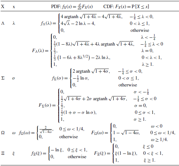


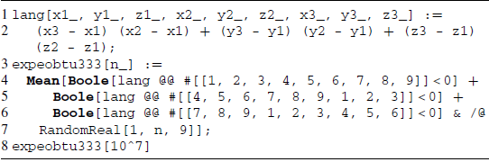


 Open access