





1. Introduction
Water waves are a ubiquitous natural phenomenon of both scientific and practical importance to mathematicians, physicists and engineers. Due to their intrinsic nonlinearity, numerical simulations play an indispensable role in uncovering and understanding the underlying mechanisms. Although most real-world water waves are irregular and random, much insight can be gained by studying some simple and deterministic solutions such as travelling waves and standing waves, which serve as fundamental building blocks for more complex phenomena.
Two-dimensional standing water waves have been extensively investigated through rigorous analysis, weakly nonlinear theory, fully nonlinear simulations, and laboratory experiments. Plotnikov & Toland (Reference Plotnikov and Toland2001) and Iooss, Plotnikov & Toland (Reference Iooss, Plotnikov and Toland2005) proved the existence of small-amplitude gravity standing waves in finite and infinite depth, respectively. The Stokes-type expansions of gravity standing waves were derived by Rayleigh (Reference Rayleigh1915) and Penney & Price (Reference Penney and Price1952) for deep water and by Tadjbakhsh & Keller (Reference Tadjbakhsh and Keller1960) for finite-depth water, and later extended to include surface tension by Concus (Reference Concus1962) and Vanden-Broeck (Reference Vanden-Broeck1984). In recent years, direct numerical computations on two-dimensional standing waves have received more attention in studying the branching phenomenon (Okamura Reference Okamura1985; Mercer & Roberts Reference Mercer and Roberts1994; Smith & Roberts Reference Smith and Roberts1999; Wilkening & Yu Reference Wilkening and Yu2012; Shelton, Milewski & Trinh Reference Shelton, Milewski and Trinh2023), the mechanisms of instability (Mercer & Roberts Reference Mercer and Roberts1992; Bryant & Stiassnie Reference Bryant and Stiassnie1994; Wilkening Reference Wilkening2020), and the long-standing conjecture on the limiting configuration of gravity standing waves (Mercer & Roberts Reference Mercer and Roberts1992; Okamura Reference Okamura1998, Reference Okamura2003, Reference Okamura2010; Schultz et al. Reference Schultz, Vanden-Broeck, Jiang and Perlin1998; Wilkening Reference Wilkening2011; Wilkening & Yu Reference Wilkening and Yu2012). Three principal numerical approaches have been established: (i) spatio-temporal collocation methods based on the Fourier and other spectral expansions (Vanden-Broeck & Schwartz Reference Vanden-Broeck and Schwartz1981; Tsai & Yue Reference Tsai and Yue1987; Tsai & Jeng Reference Tsai and Jeng1994; Bryant & Stiassnie Reference Bryant and Stiassnie1994, Reference Bryant and Stiassnie1995; Okamura Reference Okamura2003); (ii) semi-analytic series-expansion methods (Schwartz & Whitney Reference Schwartz and Whitney1981; Rottman Reference Rottman1982; Abassi & Wilkening Reference Abassi and Wilkening2025); and (iii) time-dependent methods (usually via the boundary-integral formulation) combined with Newton or nonlinear least squares solvers (Mercer & Roberts Reference Mercer and Roberts1992; Schultz et al. Reference Schultz, Vanden-Broeck, Jiang and Perlin1998; Wilkening Reference Wilkening2011; Wilkening & Yu Reference Wilkening and Yu2012; Shelton et al. Reference Shelton, Milewski and Trinh2023). The last approach is most commonly used owing to its relatively low computational cost, although the time integration may suffer from numerical instabilities, aliasing errors and filtering errors. In contrast, the spatio-temporal collocation methods avoid these issues and guarantee exact temporal periodicity owing to the Fourier expansion in time. When the system is stiff or chaotic, this approach is particularly attractive, despite the heavy computational cost in solving large-scale algebraic systems. Such an issue had limited the application of spatio-temporal collocation methods in early years, but is largely alleviated over the past decades with a rapid growth of computational power.
In contrast, three-dimensional standing waves have received considerably less attention, and the existing works were primarily concerned with gravity waves based on weakly nonlinear theory in studying the Stokes-type expansion (Verma & Keller Reference Verma and Keller1962), bifurcation (Bridges Reference Bridges1987) and linear stability (Okamura Reference Okamura1985; Bryant & Stiassnie Reference Bryant and Stiassnie1995). Direct computation of nonlinear three-dimensional standing waves remains highly challenging, despite the recent progress (Tsai & Yue Reference Tsai and Yue1987; Bryant & Stiassnie Reference Bryant and Stiassnie1995; Zhu, Liu & Yue Reference Zhu, Liu and Yue2003; Rycroft & Wilkening Reference Rycroft and Wilkening2013). Of particular interest, Bryant & Stiassnie (Reference Bryant and Stiassnie1995) and Zhu et al. (Reference Zhu, Liu and Yue2003) showed that two-dimensional standing waves may be unstable to transverse and oblique disturbances whose frequencies are close to that of the base standing waves. Note that in the linear sense, a three-dimensional standing wave can be decomposed into two obliquely oriented standing waves:
 \begin{align} \cos (kx)\cos (ly)\cos (\omega t) = \frac {1}{2}\cos (kx+ly)\cos (\omega t) + \frac {1}{2}\cos (kx-ly)\cos (\omega t), \end{align}
where $k$
and
$k$
and $l$
denote the wavenumbers in the
$l$
denote the wavenumbers in the $x$
- and
$x$
- and $y$
-directions, and
$y$
-directions, and $\omega$
is the nonlinear frequency. If one of the two components is slightly disturbed, then the instability found by Zhu et al. (Reference Zhu, Liu and Yue2003) suggests that energy could flow between these two components cyclically, leading to a recurrence phenomenon over long temporal periods. In this paper, we present some numerical evidence supporting this assertion. On the other hand, all these mentioned works neglected surface tension, which is known to give rise to various non-trivial effects on water waves (Perlin & Schultz Reference Perlin and Schultz2000) by modifying the dispersion relation. In particular, it changes the dominant resonance mechanism from four-wave to three-wave interactions, therefore accelerating energy cascade rate. Such resonances lead to the classical Wilton ripples, travelling gravity-capillary waves whose fundamental and second-order spatial harmonics have comparable amplitudes and propagate at the same speed. For standing waves, the effect of surface tension has been investigated only in two dimensions (Vanden-Broeck Reference Vanden-Broeck1984; Schultz et al. Reference Schultz, Vanden-Broeck, Jiang and Perlin1998; Wilkening & Yu Reference Wilkening and Yu2012; Shelton et al. Reference Shelton, Milewski and Trinh2023), thereby motivating the present work to study more complex, non-collinear resonant modes in three dimensions.
$\omega$
is the nonlinear frequency. If one of the two components is slightly disturbed, then the instability found by Zhu et al. (Reference Zhu, Liu and Yue2003) suggests that energy could flow between these two components cyclically, leading to a recurrence phenomenon over long temporal periods. In this paper, we present some numerical evidence supporting this assertion. On the other hand, all these mentioned works neglected surface tension, which is known to give rise to various non-trivial effects on water waves (Perlin & Schultz Reference Perlin and Schultz2000) by modifying the dispersion relation. In particular, it changes the dominant resonance mechanism from four-wave to three-wave interactions, therefore accelerating energy cascade rate. Such resonances lead to the classical Wilton ripples, travelling gravity-capillary waves whose fundamental and second-order spatial harmonics have comparable amplitudes and propagate at the same speed. For standing waves, the effect of surface tension has been investigated only in two dimensions (Vanden-Broeck Reference Vanden-Broeck1984; Schultz et al. Reference Schultz, Vanden-Broeck, Jiang and Perlin1998; Wilkening & Yu Reference Wilkening and Yu2012; Shelton et al. Reference Shelton, Milewski and Trinh2023), thereby motivating the present work to study more complex, non-collinear resonant modes in three dimensions.
A central difficulty in simulating water waves lies within resolving the non-local relationship between the normal and tangential velocities on the free surface. This is commonly achieved by solving Laplace’s equation subject to suitable boundary conditions. However, directly solving Laplace’s equation in a three-dimensional fluid domain requires efficient multigrid algorithms to remain computationally tractable (Rycroft & Wilkening Reference Rycroft and Wilkening2013). In contrast, the boundary-integral method is widely employed owing to its ability to reduce the dimensionality of the problem. Despite its superior numerical efficiency, the three-dimensional boundary-integral formulation presents additional difficulty in handling the slowly converging lattice sums due to the absence of a closed-form integral kernel. To address these difficulties, we adopt a third approach based on Zakharov’s Hamiltonian formulation of water waves (Zakharov Reference Zakharov1968) and the Dirichlet–Neumann operator (DNO). This method is computationally efficient because it provides explicit and systematic approximations to the non-local relationship of the full potential-flow problem. Therefore, it is widely used in water-wave problems (Craig & Sulem Reference Craig and Sulem1993; Nicholls Reference Nicholls1998; Craig & Nicholls Reference Craig and Nicholls2000, Reference Craig and Nicholls2002; Xu & Guyenne Reference Xu and Guyenne2009; Wang & Milewski Reference Wang and Milewski2012; Wang, Milewski & Vanden-Broeck Reference Wang, Milewski and Vanden-Broeck2014; Wilkening & Zhao Reference Wilkening and Zhao2021; Guan & Wang Reference Guan and Wang2022; Xu & Wang Reference Xu and Wang2025). The key steps of this method are to truncate the DNO in the Hamiltonian of the system, and then take variational derivatives with respect to the surface elevation $\eta$
and the surface velocity potential
$\eta$
and the surface velocity potential $\varphi$
, which lead to reduced models of the full water-wave problem. Alternatively, one can first take the variational derivatives of the exact Hamiltonian, which gives rise to the kinematic and dynamic boundary conditions, and then truncate the DNO. Note that even when truncated to the same order, the two approaches usually give different high-order terms in their resulting models. It is worth mentioning that Ambrose, Bona & Nicholls (Reference Ambrose, Bona and Nicholls2014) have shown evidence that the second- and third-order truncations for deep-water gravity waves are likely ill-posed. It is argued that by including the effect of surface tension, a well-posed model can be formed. This seems to align with our numerical tests because we never encountered such ill-posedness issue in our temporal simulations. In the present paper, we follow Wang & Milewski (Reference Wang and Milewski2012) and Wang et al. (Reference Wang, Milewski and Vanden-Broeck2014) who employed the third- and fifth-order truncations through the first approach to study gravity-capillary and flexural-gravity solitary waves, respectively. A novelty of their models is the fully nonlinear form of the surface-tension or flexural-tension terms, which provide considerably better agreement to the full potential-flow formulation. Because of the numerical stiffness introduced by surface tension, initial-value calculations for three-dimensional gravity-capillary standing waves are computationally intensive. Therefore, we develop a boundary-value algorithm based on the spatio-temporal collocation methods that were previously used in two dimensions. By exploiting a large amount of spatio-temporal symmetries, we reduce the number of unknowns by a factor of 64, then solve the problem in physical space via Newton’s method. Nevertheless, the numerical computation is still intensive and is therefore performed on a 128-core compute node equipped with AMD EPYC 7742 processors. Typically, executing one Newton iteration takes
$\varphi$
, which lead to reduced models of the full water-wave problem. Alternatively, one can first take the variational derivatives of the exact Hamiltonian, which gives rise to the kinematic and dynamic boundary conditions, and then truncate the DNO. Note that even when truncated to the same order, the two approaches usually give different high-order terms in their resulting models. It is worth mentioning that Ambrose, Bona & Nicholls (Reference Ambrose, Bona and Nicholls2014) have shown evidence that the second- and third-order truncations for deep-water gravity waves are likely ill-posed. It is argued that by including the effect of surface tension, a well-posed model can be formed. This seems to align with our numerical tests because we never encountered such ill-posedness issue in our temporal simulations. In the present paper, we follow Wang & Milewski (Reference Wang and Milewski2012) and Wang et al. (Reference Wang, Milewski and Vanden-Broeck2014) who employed the third- and fifth-order truncations through the first approach to study gravity-capillary and flexural-gravity solitary waves, respectively. A novelty of their models is the fully nonlinear form of the surface-tension or flexural-tension terms, which provide considerably better agreement to the full potential-flow formulation. Because of the numerical stiffness introduced by surface tension, initial-value calculations for three-dimensional gravity-capillary standing waves are computationally intensive. Therefore, we develop a boundary-value algorithm based on the spatio-temporal collocation methods that were previously used in two dimensions. By exploiting a large amount of spatio-temporal symmetries, we reduce the number of unknowns by a factor of 64, then solve the problem in physical space via Newton’s method. Nevertheless, the numerical computation is still intensive and is therefore performed on a 128-core compute node equipped with AMD EPYC 7742 processors. Typically, executing one Newton iteration takes $1.5$
h and requires
$1.5$
h and requires $32$
GB memory for constructing a Jacobian matrix on
$32$
GB memory for constructing a Jacobian matrix on $128\times 128\times 128$
grid points. For most computations presented in this paper, this resolution is good enough to give highly accurate solutions.
$128\times 128\times 128$
grid points. For most computations presented in this paper, this resolution is good enough to give highly accurate solutions.
The remainder of the paper is organised as follows. Section 2 gives the full potential-flow and Hamiltonian formulations for three-dimensional deep-water gravity-capillary waves. Section 3 details the numerical method based on a triple boundary-value calculation. Section 4 validates the numerical accuracy and exhibits typical standing-wave solutions and bifurcations under resonances. Section 5 exhibits temporal simulations for the computed standing waves, and examines their stability. Finally, § 6 provides concluding remarks.
2. Formulations of deep-water gravity-capillary waves
We consider the mathematical formulation of deep-water gravity-capillary waves, which requires solving the velocity potential $\phi (x,y,z,t)$
and surface elevation
$\phi (x,y,z,t)$
and surface elevation $\eta (x,y,t)$
from
$\eta (x,y,t)$
from
 \begin{align} \begin{cases} {\nabla} ^2\phi +\phi _{zz} = 0 &\text{for } \ {-\infty} \lt z\lt \eta (x,y,t),\\[9pt] \eta _t + \boldsymbol{\nabla }\phi \boldsymbol{\cdot }\boldsymbol{\nabla }\eta = \phi _z & \text{at } \ z = \eta (x,y,t),\\[9pt] \phi _t + \dfrac {1}{2}\big (|\boldsymbol{\nabla }\phi |^2 + \phi _z^2\big ) + \eta = \boldsymbol{\nabla }\boldsymbol{\cdot }\Bigg (\dfrac {\boldsymbol{\nabla }\eta }{\sqrt {1+|\boldsymbol{\nabla }\eta |^2}}\Bigg ) & \text{at } \ z = \eta (x,y,t),\\[9pt] \phi _x,\phi _y,\phi _z \rightarrow 0 & \text{as } \ z\rightarrow -\infty , \end{cases} \end{align}
where $x,y$
are the horizontal Cartesian coordinates,
$x,y$
are the horizontal Cartesian coordinates, $z$
is the vertical coordinate pointing opposite to the direction of gravity,
$z$
is the vertical coordinate pointing opposite to the direction of gravity, $t$
denotes time, and
$t$
denotes time, and $\boldsymbol{\nabla }= (\partial _x,\partial _y)$
. For convenience, we put the
$\boldsymbol{\nabla }= (\partial _x,\partial _y)$
. For convenience, we put the $(x,y)$
-plane on the mean water level. Without loss of generality, we have non-dimensionalised the system by choosing the typical scalings of length, time and mass such that the gravitational acceleration, fluid density and surface tension coefficient become unit. For real water whose surface tension coefficient equals
$(x,y)$
-plane on the mean water level. Without loss of generality, we have non-dimensionalised the system by choosing the typical scalings of length, time and mass such that the gravitational acceleration, fluid density and surface tension coefficient become unit. For real water whose surface tension coefficient equals $72$
dyn cm−1,
$72$
dyn cm−1, $2\pi$
spatial units and one temporal unit correspond to
$2\pi$
spatial units and one temporal unit correspond to $1.7$
cm and
$1.7$
cm and $0.0167$
s physically.
$0.0167$
s physically.
Zakharov (Reference Zakharov1968) proved that the above formulation is equivalent to Hamilton’s canonical equations
 \begin{align} \eta _t = \dfrac {\delta \mathcal H}{\delta \varphi },\quad \varphi _t = -\dfrac {\delta \mathcal H}{\delta \eta }, \end{align}
where $\varphi (x,y,t) = \phi (x,y,\eta (x,y,t),t)$
, and the Hamiltonian
$\varphi (x,y,t) = \phi (x,y,\eta (x,y,t),t)$
, and the Hamiltonian $\mathcal H$
is the total energy of the system:
$\mathcal H$
is the total energy of the system:
 \begin{align} \mathcal H = \iint \bigg (\frac {1}{2}\varphi\, G(\eta )\, \varphi +\frac {1}{2}\eta ^2 + \sqrt {1+|\boldsymbol{\nabla }\eta |^2}-1\bigg ) \,\mathrm dx\,\mathrm dy. \end{align}
Here, $G(\eta )$
is the scaled DNO and is formally defined by
$G(\eta )$
is the scaled DNO and is formally defined by
 \begin{align} G(\eta )\varphi = \phi _{\boldsymbol{n}}\sqrt {1+|\boldsymbol{\nabla }\eta |^2}, \end{align}
where $\phi _{\boldsymbol{n}}$
is the normal derivative of
$\phi _{\boldsymbol{n}}$
is the normal derivative of $\phi$
in the outward direction to the surface. It is rigorously proved that the DNO has a convergent Taylor series
$\phi$
in the outward direction to the surface. It is rigorously proved that the DNO has a convergent Taylor series
 \begin{align} G(\eta ) = \sum _{i=0}^{\infty } G_i(\eta ), \end{align}
provided that the norm of $\eta$
is smaller than a certain constant (Coifman & Meyer Reference Coifman and Meyer1985; Craig & Nicholls Reference Craig and Nicholls2000). For the convenience of numerical computation, the expressions for
$\eta$
is smaller than a certain constant (Coifman & Meyer Reference Coifman and Meyer1985; Craig & Nicholls Reference Craig and Nicholls2000). For the convenience of numerical computation, the expressions for $G_i$
are commonly written in a recursive form (Craig & Sulem Reference Craig and Sulem1993; Craig & Nicholls Reference Craig and Nicholls2002); see Appendix A. By truncating the DNO to a certain order
$G_i$
are commonly written in a recursive form (Craig & Sulem Reference Craig and Sulem1993; Craig & Nicholls Reference Craig and Nicholls2002); see Appendix A. By truncating the DNO to a certain order $n$
, one obtains an approximated Hamiltonian. Substituting it into (2.2) leads to a
$n$
, one obtains an approximated Hamiltonian. Substituting it into (2.2) leads to a $n$
th-order truncated model
$n$
th-order truncated model
 \begin{align} \eta _t & = \sum _{i=0}^{n-1} G_i(\eta )\,\varphi , \\[-12pt]\nonumber \end{align}
 \begin{align} \varphi _t &= \sum _{i=2}^{n}\mathcal N_i(\eta ,\varphi ) - \eta + \boldsymbol{\nabla }\boldsymbol{\cdot }\Bigg ( \frac {\boldsymbol{\nabla }\eta }{\sqrt {1+|\boldsymbol{\nabla }\eta |^2}}\Bigg ), \end{align}
where $\mathcal N_i$
represents the DNO-involved
$\mathcal N_i$
represents the DNO-involved $i$
th-order nonlinear term whose expression can be found in Appendix A. Wang & Milewski (Reference Wang and Milewski2012) and Wang et al. (Reference Wang, Milewski and Vanden-Broeck2014) employed cubic (
$i$
th-order nonlinear term whose expression can be found in Appendix A. Wang & Milewski (Reference Wang and Milewski2012) and Wang et al. (Reference Wang, Milewski and Vanden-Broeck2014) employed cubic ( $n=3$
) and quintic (
$n=3$
) and quintic ( $n=5$
) truncations (denoted by cubic model and quintic model hereafter) to study gravity-capillary and flexural-gravity solitary waves, respectively. They showed that these models are quite accurate compared with the original water-wave formulation, even when solutions have large amplitudes. In the following sections, we investigate three-dimensional gravity-capillary standing waves in rectangular or square basins by searching for triply periodic (in the
$n=5$
) truncations (denoted by cubic model and quintic model hereafter) to study gravity-capillary and flexural-gravity solitary waves, respectively. They showed that these models are quite accurate compared with the original water-wave formulation, even when solutions have large amplitudes. In the following sections, we investigate three-dimensional gravity-capillary standing waves in rectangular or square basins by searching for triply periodic (in the $x,y$
and
$x,y$
and $t$
directions) solutions of the cubic and quintic models.
$t$
directions) solutions of the cubic and quintic models.
3. Spatio-temporal collocation method
3.1. Linear solutions
By solving the linearised water-wave equations, one obtains the linear standing-wave solution
 \begin{align} \begin{cases} \widetilde {\eta }_{k,l}(x,y,t) = \cos (k x)\cos (l y)\cos (\omega t), \\[5pt] \widetilde {\varphi }_{k,l}(x,y,t) = -\dfrac {\omega }{\kappa } \cos (kx)\cos (l y)\sin (\omega t), \end{cases} \end{align}
where $\kappa = \sqrt {k^2+l^2}$
, and
$\kappa = \sqrt {k^2+l^2}$
, and $\omega$
satisfies the dispersion relation for deep-water gravity-capillary waves,
$\omega$
satisfies the dispersion relation for deep-water gravity-capillary waves,
 \begin{align} \omega ^2 = \kappa + \kappa ^3. \end{align}
We use the following two assumptions when computing standing waves:
-
(i) $\varphi = 0$
at
$t = 0,T/2,T,3T/2,\ldots$
,
$\varphi = 0$
at
$t = 0,T/2,T,3T/2,\ldots$
, -
(ii)
$\eta$
and
$\varphi$
are even functions of
$x$
and
$y$
,


where $T$
is the smallest temporal period. The first assumption implies that the kinetic energy vanishes every half-period. Although this also seems true for potential energy because
$T$
is the smallest temporal period. The first assumption implies that the kinetic energy vanishes every half-period. Although this also seems true for potential energy because $\widetilde {\eta }_{k,l}$
vanishes periodically in time, the potential energy of nonlinear standing waves never vanishes, as will be shown later. To construct standing waves in rectangular or square basins, we use the following three types of linear solutions.
$\widetilde {\eta }_{k,l}$
vanishes periodically in time, the potential energy of nonlinear standing waves never vanishes, as will be shown later. To construct standing waves in rectangular or square basins, we use the following three types of linear solutions.
-
(i) Case I (rectangular basin):
$\eta = \epsilon \widetilde {\eta }_{k,l},\ \varphi = \epsilon \widetilde {\varphi }_{k,l}$
,
$k,l\neq 0,\ k\neq l$
. -
(ii) Case II (square basin):
$\eta = \epsilon \widetilde {\eta }_{k,l} + \epsilon \widetilde {\eta }_{l,k},\ \varphi = \epsilon \widetilde {\varphi }_{k,l} + \epsilon \widetilde {\varphi }_{l,k}$
,
$l = rk,\ r = 1,3,5,\ldots$
. -
(iii) Case III (square basin):
$\eta = \epsilon \widetilde {\eta }_{k,l} + \epsilon \widetilde {\eta }_{l,k},\ \varphi = \epsilon \widetilde {\varphi }_{k,l} + \epsilon \widetilde {\varphi }_{l,k}$
,
$l = rk,\ r = 0,2,4,\ldots$
.


Here, $\epsilon$
is a small parameter. To support standing waves in square basins, it is required that
$\epsilon$
is a small parameter. To support standing waves in square basins, it is required that $k$
and
$k$
and $l$
be rationally related, but we only study the case that
$l$
be rationally related, but we only study the case that $l$
is an integer multiple of
$l$
is an integer multiple of $k$
. In general, one can also consider the following form of linear solution:
$k$
. In general, one can also consider the following form of linear solution:
 \begin{align} \eta = \epsilon \widetilde {\eta }_{k,rk} - \epsilon \widetilde {\eta }_{rk,k},\quad\varphi = \epsilon \widetilde {\varphi }_{k,rk} - \epsilon \widetilde {\varphi }_{rk,k}. \end{align}
For $r = 0,2,4,\ldots$
and
$r = 0,2,4,\ldots$
and $y = Y+\pi /k$
, we have
$y = Y+\pi /k$
, we have
 \begin{align} \cos (kx)\cos (rk y)-\cos (rkx)\cos (k y) = \cos (kx)\cos (rk Y)+\cos (rkx)\cos (k Y), \end{align}
thus (3.3) is equivalent to case III without specifying additional symmetries. On the other hand, for $r=1,3,5,\ldots$
, we find no convergent solution using (3.3). Note that
$r=1,3,5,\ldots$
, we find no convergent solution using (3.3). Note that
 \begin{align} \widetilde {\eta }_{k,l}(x,y,t) = \frac {1}{2}\widetilde {\eta }_{\kappa ,0}(\xi ,\zeta ,t) + \frac {1}{2}\widetilde {\eta }_{0,\kappa }(\xi ,\zeta ,t), \end{align}
where $\xi = (kx+ly)/\kappa$
and
$\xi = (kx+ly)/\kappa$
and $\zeta = (kx-ly)/\kappa$
. This means that a three-dimensional standing wave can be decomposed into obliquely oriented two-dimensional standing waves, at least linearly. In particular, when
$\zeta = (kx-ly)/\kappa$
. This means that a three-dimensional standing wave can be decomposed into obliquely oriented two-dimensional standing waves, at least linearly. In particular, when $k=l$
, a case II standing wave can be transformed to a case III standing wave by rotating the
$k=l$
, a case II standing wave can be transformed to a case III standing wave by rotating the $(x,y)$
-plane by
$(x,y)$
-plane by $\pi /4$
.
$\pi /4$
.
3.2. Spatio-temporal symmetries
We consider triply periodic solutions in a three-dimensional cube
 \begin{align} \{(x,y,t)\mid -L_1\le x\le L_1,\, -L_2\le y\le L_2,\, 0\le t \le T\}, \end{align}
where $2L_1$
and
$2L_1$
and $2L_2$
are the smallest periods in the
$2L_2$
are the smallest periods in the $x$
- and
$x$
- and $y$
-directions. Using the time-reversal argument, solutions must have a temporal symmetry about
$y$
-directions. Using the time-reversal argument, solutions must have a temporal symmetry about $t = T/2$
:
$t = T/2$
:
 \begin{align} \eta (x,y,T/2-t') &= \eta (x,y,T/2+t'), \\[-12pt]\nonumber \end{align}
 \begin{align} \varphi (x,y,T/2-t') &= -\varphi (x,y,T/2+t'), \end{align}
where $t'\in \mathbb R$
. Since
$t'\in \mathbb R$
. Since $\varphi$
vanishes at
$\varphi$
vanishes at $t = T/2$
,
$t = T/2$
, $\eta$
must returns to its initial state with a spatial shift (we do not consider other possibilities in this paper). Otherwise,
$\eta$
must returns to its initial state with a spatial shift (we do not consider other possibilities in this paper). Otherwise, $T/2$
becomes the smallest temporal period. To ensure consistency with linear solutions, there exist two types of shift.
$T/2$
becomes the smallest temporal period. To ensure consistency with linear solutions, there exist two types of shift.
-
(i) For cases I and II,
(3.9)
\begin{align} \eta (x,y,0) = \eta (x\pm L_1,y,T/2) = \eta (x,y\pm L_2,T/2). \end{align}
-
(ii) For case III,
(3.10)
\begin{align} \eta (x,y,0) = \eta (x\pm L_1,y\pm L_2,T/2). \end{align}


Using the time-reversal argument again, solutions must be symmetric about $t = T/4$
.
$t = T/4$
.
-
(i) For cases I and II,
(3.11)
\begin{align} \eta (x,y,T/4-t') &= \eta (x\pm L_1,y,T/4+t') = \eta (x,y\pm L_2,T/4+t'), \\[-12pt]\nonumber \end{align}
(3.12)
\begin{align} \varphi (x,y,T/4-t') &= -\varphi (x\pm L_1,y,T/4+t') = -\varphi (x,y\pm L_2,T/4+t'). \end{align}
-
(ii) For case III,
(3.13)
\begin{align} \eta (x,y,T/4-t') &= \eta (x\pm L_1,y\pm L_2,T/4+t'), \\[-12pt]\nonumber \end{align}
(3.14)
\begin{align} \varphi (x,y,T/4-t') &= -\varphi (x\pm L_1,y\pm L_2,T/4+t'). \end{align}


Consequently, we only need to consider a quarter temporal period, say $0\le t\le T/4$
, in computation.
$0\le t\le T/4$
, in computation.
Owing to the even symmetry with respect to $x$
and
$x$
and $y$
(termed fourfold symmetry hereafter), i.e.
$y$
(termed fourfold symmetry hereafter), i.e.
 \begin{align} \eta (x,y,t) &= \eta (-x,y,t) = \eta (-x,-y,t) = \eta (x,-y,t), \\[-12pt]\nonumber \end{align}
 \begin{align} \varphi (x,y,t) &= \varphi (-x,y,t) = \varphi (-x,-y,t) = \varphi (x,-y,t), \end{align}
we only need to consider the values of $\eta$
and
$\eta$
and $\varphi$
within one quadrant, say
$\varphi$
within one quadrant, say $\{(x,y,t)\mid -L_1\le x\le 0,\ {-L_2}\le y\le 0,\ 0\le t\le T/4\}$
. For cases I and II, (3.11)–(3.12) imply
$\{(x,y,t)\mid -L_1\le x\le 0,\ {-L_2}\le y\le 0,\ 0\le t\le T/4\}$
. For cases I and II, (3.11)–(3.12) imply
 \begin{align} \eta (x,y,t) &= \eta (x\pm L_1,y\pm L_2,t), \\[-12pt]\nonumber \end{align}
 \begin{align} \varphi (x,y,t) &= \varphi (x\pm L_1,y\pm L_2,t). \end{align}
Combining these with the fourfold symmetry, we have
 \begin{align} \eta (-x,-y,t) &= \eta (x\pm L_1,y\pm L_2,t), \\[-12pt]\nonumber \end{align}
 \begin{align} \varphi (-x,-y,t) &= \varphi (x\pm L_1,y\pm L_2,t). \end{align}
This property is used for case I standing waves to reduce the number of unknowns, as shown in figure 1.


For cases II and III, solutions have a stronger eightfold symmetry, i.e. fourfold symmetry plus even symmetry about the two diagonals $x=\pm y$
:
$x=\pm y$
:
 \begin{align} \eta (x,y,t) &= \eta (y,x,t)= \eta (-y,-x,t), \\[-12pt]\nonumber \end{align}
 \begin{align} \varphi (x,y,t) &= \varphi (y,x,t)= \varphi (-y,-x,t). \end{align}
Combining these with (3.17) and (3.18), we have the following identities for case II:
 \begin{align} \eta (x,y,t) &= \eta (y\pm L,x\mp L,t) = \eta (-y\pm L,-x\mp L,t), \\[-12pt]\nonumber \end{align}
 \begin{align} \varphi (x,y,t) &= \varphi (y\pm L,x\mp L,t) = \varphi (-y\pm L,-x\mp L,t), \end{align}
where $L = L_1 = L_2$
. This means that case II solutions are also symmetric about the four straight lines
$L = L_1 = L_2$
. This means that case II solutions are also symmetric about the four straight lines $x+y = \pm L$
,
$x+y = \pm L$
, $x-y = \pm L$
. We use these symmetries to reduce the computational domain from a quadrant to one of its quarter sub-triangles, as shown in figure 2. For case III, however, solutions are only symmetric about the two diagonals, as shown in figure 3. Moreover, there exist additional spatial symmetries for all three cases at
$x-y = \pm L$
. We use these symmetries to reduce the computational domain from a quadrant to one of its quarter sub-triangles, as shown in figure 2. For case III, however, solutions are only symmetric about the two diagonals, as shown in figure 3. Moreover, there exist additional spatial symmetries for all three cases at $t=T/4$
. Setting
$t=T/4$
. Setting $t' = 0$
in (3.11)–(3.14) and using the fourfold symmetry, we have the following.
$t' = 0$
in (3.11)–(3.14) and using the fourfold symmetry, we have the following.
Typical contours of $\eta$
for a case II standing wave. The squares surrounded by the black dashed and solid lines represent a unit periodic cell and a quadrant on the
$\eta$
for a case II standing wave. The squares surrounded by the black dashed and solid lines represent a unit periodic cell and a quadrant on the $(x,y)$
-plane, respectively. The blue straight lines show the two diagonals
$(x,y)$
-plane, respectively. The blue straight lines show the two diagonals $x = \pm y$
, and the four red straight lines denote
$x = \pm y$
, and the four red straight lines denote $x+y = \pm L$
and
$x+y = \pm L$
and $x-y = \pm L$
. The shaded region denotes the real computational domain by using (3.23) and (3.24).
$x-y = \pm L$
. The shaded region denotes the real computational domain by using (3.23) and (3.24).

Typical contours of $\eta$
for a case III standing wave. The squares surrounded by the black dashed and solid lines represent a unit periodic cell and a quadrant on the
$\eta$
for a case III standing wave. The squares surrounded by the black dashed and solid lines represent a unit periodic cell and a quadrant on the $(x,y)$
-plane, respectively. The blue straight lines show the two diagonals
$(x,y)$
-plane, respectively. The blue straight lines show the two diagonals $x = \pm y$
. The shaded region denotes the real computational domain by using (3.21) and (3.22).
$x = \pm y$
. The shaded region denotes the real computational domain by using (3.21) and (3.22).

Figure 3. Long description
Panel A: A contour plot representing a case III standing wave. The plot features blue and red contour lines indicating wave patterns. The black dashed and solid lines form a square representing a unit periodic cell and a quadrant on the x-y plane, respectively. The blue straight lines depict the two diagonals of the square. The axes are labeled x and y. Panel B: A zoomed-in view of the shaded region from Panel A, showing detailed contour lines within the real computational domain. The axes are also labeled x and y.
-
(i) For cases I and II,
(3.25)
\begin{align} \eta (-x,y,T/4) &= \eta (x\pm L_1,y,T/4) = \eta (x,y\pm L_2,T/4) = \eta (x,-y,T/4), \\[-12pt]\nonumber \end{align}
(3.26)
\begin{align} \varphi (-x,y,T/4) &= -\varphi (x\pm L_1,y,T/4) = -\varphi (x,y\pm L_2,T/4) = \varphi (x,-y,T/4). \end{align}
-
(ii) For case III,
(3.27)
\begin{align} \eta (-x,-y,T/4) &= \eta (x\pm L_1,y\pm L_2,T/4), \\[-12pt]\nonumber \end{align}
(3.28)
\begin{align} \varphi (-x,-y,T/4) &= -\varphi (x\pm L_1,y\pm L_2,T/4). \end{align}


This means that at $t = T/4$
, case I and case II solutions are symmetric about
$t = T/4$
, case I and case II solutions are symmetric about $x = \pm L_1/2$
and
$x = \pm L_1/2$
and $y = \pm L_2/2$
within each quadrant, and case III solutions are symmetric about
$y = \pm L_2/2$
within each quadrant, and case III solutions are symmetric about $x+y = \pm L$
and
$x+y = \pm L$
and $x-y = \pm L$
, as shown in figure 4.
$x-y = \pm L$
, as shown in figure 4.
Typical contours of $\eta (x,y,T/4)$
for (a) case I, (b) case II and (c) case III standing waves. The rectangle and squares surrounded by the solid black lines each represent a quadrant on the
$\eta (x,y,T/4)$
for (a) case I, (b) case II and (c) case III standing waves. The rectangle and squares surrounded by the solid black lines each represent a quadrant on the $(x,y)$
-plane. The blue straight lines are the two diagonals
$(x,y)$
-plane. The blue straight lines are the two diagonals $x = \pm y$
. The red straight lines denote
$x = \pm y$
. The red straight lines denote $x+y = \pm L$
and
$x+y = \pm L$
and $x-y = \pm L$
. The green lines indicate
$x-y = \pm L$
. The green lines indicate $x = \pm L_1/2$
and
$x = \pm L_1/2$
and $y = \pm L_2/2$
. The shaded regions denote the real computational domain.
$y = \pm L_2/2$
. The shaded regions denote the real computational domain.

Note that the reflection symmetry imposed for standing waves is an assumption. Although it is clear that there exist asymmetric travelling-standing waves (Wilkening Reference Wilkening2021), it remains an open question regarding the existence of asymmetric standing waves.
3.3. Numerical implementation
We introduce $I+1,\ J+1$
and
$I+1,\ J+1$
and $N+1$
uniform collocation points for
$N+1$
uniform collocation points for $x,\ y$
and
$x,\ y$
and $t$
, i.e.
$t$
, i.e.
 \begin{align} x_i &= \frac{2(i-1)L_1}{I}-L_1,\quad i = 1,2,\ldots ,I+1, \\[-12pt]\nonumber \end{align}
 \begin{align} y_{\!j} &= \frac{2(j-1)L_2}{J}-L_2,\quad j = 1,2,\ldots ,J+1, \\[-12pt]\nonumber \end{align}
 \begin{align} t_n &= \frac{(n-1)T}{N},\quad n = 1,2,\ldots ,N+1, \end{align}
and our task is to solve the function values of $\eta$
and
$\eta$
and $\varphi$
at these points, along with the frequency
$\varphi$
at these points, along with the frequency $\omega$
, given wave amplitude
$\omega$
, given wave amplitude $H$
(this can be the wave amplitude in physical space, the amplitude of a fundamental Fourier mode, or a measure of energy). Based on the spatio-temporal symmetries, we have the following unknowns to solve for the case I standing waves.
$H$
(this can be the wave amplitude in physical space, the amplitude of a fundamental Fourier mode, or a measure of energy). Based on the spatio-temporal symmetries, we have the following unknowns to solve for the case I standing waves.
-
(i) At
$t=0$
,
$\eta (x_i,y_{\!j},0)$
for
$i=1,2,\ldots,I/4+1$
and
$j=1,2,\ldots,J/2+1$
. -
(ii) At
$t = t_n$
(
$n=2,3,\ldots, N/4$
),
$\eta (x_i,y_{\!j},t_n)$
and
$\varphi (x_i,y_{\!j},t_n)$
for
$i=1,2,\ldots ,I/4+1$
and
$j=1,2,\ldots ,J/2+1$
. -
(iii) At
$t=T/4$
,
$\eta (x_i,y_{\!j},T/4)$
for
$i=1,2,\ldots ,I/4+1$
and
$j=1,2,\ldots ,J/4+1$
,
$\varphi (x_i,y_{\!j},T/4)$
for
$i=1,2,\ldots ,I/4$
and
$j=1,2,\ldots ,J/4$
.





Schematic of the reduced computational domain by using spatio-temporal symmetries.

All together, these give rise to $(I/4+1)(J/2+1)N/2 - J/4 \sim IJN/16$
unknowns for
$(I/4+1)(J/2+1)N/2 - J/4 \sim IJN/16$
unknowns for $\eta$
and
$\eta$
and $\varphi$
. For cases II and III, it is convenient to let
$\varphi$
. For cases II and III, it is convenient to let $I=J$
. The total numbers of unknowns for
$I=J$
. The total numbers of unknowns for $\eta$
and
$\eta$
and $\varphi$
are reduced to
$\varphi$
are reduced to $(I/4+1)^2N/2 \sim I^2N/32$
for case II, and
$(I/4+1)^2N/2 \sim I^2N/32$
for case II, and $(I/4+1)(I/2+1)N/2 \sim I^2N/16$
for case III. A schematic is drawn in figure 5 to show the reduced computational domain for all three cases. Equations (2.6) and (2.7) give rise to the same number of equations after using the spatio-temporal symmetries. To close the system, we use the wave-amplitude equation
$(I/4+1)(I/2+1)N/2 \sim I^2N/16$
for case III. A schematic is drawn in figure 5 to show the reduced computational domain for all three cases. Equations (2.6) and (2.7) give rise to the same number of equations after using the spatio-temporal symmetries. To close the system, we use the wave-amplitude equation
 \begin{align} \eta (0,0,0) = H, \end{align}
for given values of $H$
.
$H$
.
The system is solved via Newton’s method by setting the iterative tolerance to $10^{-10}$
. The actual residuals for convergent solutions are usually several orders smaller than this value. All derivatives and operations involving the DNOs are calculated via a pseudo-spectral method and fast Fourier transform. Once we get a convergent solution, we use the continuation method to search for other solutions along the solution branch by gradually increasing
$10^{-10}$
. The actual residuals for convergent solutions are usually several orders smaller than this value. All derivatives and operations involving the DNOs are calculated via a pseudo-spectral method and fast Fourier transform. Once we get a convergent solution, we use the continuation method to search for other solutions along the solution branch by gradually increasing $H$
. In the presence of turning points, we alternatively use
$H$
. In the presence of turning points, we alternatively use $H$
and
$H$
and $\omega$
as the bifurcation parameters.
$\omega$
as the bifurcation parameters.
4. Numerical results
4.1. Comparisons with existing results
We first compare our numerical solutions with some existing results. For two-dimensional gravity-capillary standing waves in finite water depth $h$
, Concus (Reference Concus1962) derived a third-order Stokes expansion and the nonlinear dependence of
$h$
, Concus (Reference Concus1962) derived a third-order Stokes expansion and the nonlinear dependence of $\omega$
on
$\omega$
on $\epsilon$
, the amplitude of the fundamental Fourier mode. For
$\epsilon$
, the amplitude of the fundamental Fourier mode. For $k=1$
, this relation reads (using our scalings)
$k=1$
, this relation reads (using our scalings)
 \begin{align} \omega \sim \omega _0+\frac {1}{2}\epsilon ^2\omega _2 + O(\epsilon ^3), \end{align}
where
 \begin{align} \omega _0 =\sqrt {2\tanh (h)},\quad \omega _2 = \frac {-2\omega _0^5-39\omega _0-66\omega _0^{-3}+2592\omega _0^{-7}}{320(1-6\omega _0^{-4})}, \end{align}
and $\epsilon$
represents the amplitude of the
$\epsilon$
represents the amplitude of the $\cos (x)\cos (\omega t)$
mode. Figure 6 compares Concus’s asymptotic result and our numerical results of boundary-integral formulation (see Appendix B), the cubic model and the quintic model, for
$\cos (x)\cos (\omega t)$
mode. Figure 6 compares Concus’s asymptotic result and our numerical results of boundary-integral formulation (see Appendix B), the cubic model and the quintic model, for $k = 1, h = \infty$
. Figure 6(a) exhibits the bifurcation curve plotted under
$k = 1, h = \infty$
. Figure 6(a) exhibits the bifurcation curve plotted under $\omega$
and
$\omega$
and $\epsilon$
. All results show perfect consistency and are indistinguishable when
$\epsilon$
. All results show perfect consistency and are indistinguishable when $\epsilon \lt 0.2$
. As
$\epsilon \lt 0.2$
. As $\epsilon$
gradually increases towards
$\epsilon$
gradually increases towards $0.4$
, the cubic model agrees well with Concus’s analytic result, while the quintic model gives almost identical results to the boundary-integral method, indicated by both the frequency curves and the wave profiles in figure 6(b).
$0.4$
, the cubic model agrees well with Concus’s analytic result, while the quintic model gives almost identical results to the boundary-integral method, indicated by both the frequency curves and the wave profiles in figure 6(b).
Comparisons between Concus’s asymptotic result (4.1), and the numerical results using the boundary-integral method, the cubic model and the quintic model for $k=1, h=\infty$
. (a) Plot of
$k=1, h=\infty$
. (a) Plot of $\omega$
versus
$\omega$
versus $\epsilon$
. (b) Initial wave profiles with crest-to-trough amplitude
$\epsilon$
. (b) Initial wave profiles with crest-to-trough amplitude $0.8$
(
$0.8$
( $\epsilon = 0.394$
).
$\epsilon = 0.394$
).

Figure 6. Long description
Panel A: A line graph plots omega against epsilon. The x-axis represents epsilon ranging from 0 to 0.4, and the y-axis represents omega ranging from 1.35 to 1.42. The graph includes four data series: Boundary integrals, Concus, Cubic model, and Quintic model. All data series show a decreasing trend as epsilon increases. Panel B: A line graph plots eta(x, 0) against x. The x-axis represents x ranging from negative pi to pi, and the y-axis represents eta(x, 0) ranging from negative 0.5 to 0.5. The graph includes four data series: Boundary integrals, Concus, Cubic model, and Quintic model. All data series show a wave-like pattern with a peak at x equals 0 and troughs at x equals negative pi and pi. An inset zooms in on the region from negative 0.5 to 0.5 on the x-axis and from 0.31 to 0.34 on the y-axis, showing detailed differences among the models.
Another comparison is made for the case II three-dimensional gravity standing waves in finite-depth water. Verma & Keller (Reference Verma and Keller1962) derived the second-order Stokes-type expansion and the asymptotic expression for the nonlinear frequency, which has the same form as (4.1). For $k=l=1$
, the coefficients are
$k=l=1$
, the coefficients are
 \begin{align} \omega _0 = \sqrt {\sqrt {2}\tanh (\sqrt {2}h)},\quad \omega _2 = -\frac {(3\omega _0^4-2)^2}{16\omega _0(\tanh (2h)-2\omega _0^2)} + \frac {36\omega _0^{-7}-24\omega _0^{-3}+5\omega _0-23\omega _0^{5}}{64}, \end{align}
and $\epsilon$
represents the amplitude of
$\epsilon$
represents the amplitude of $\cos (x)\cos (y)\cos (\omega t)$
. Figure 7(a) compares the numerical results obtained from the the cubic and quintic models, the asymptotic result of Verma & Keller (Reference Verma and Keller1962), and the numerical result of Rycroft & Wilkening (Reference Rycroft and Wilkening2013), for
$\cos (x)\cos (y)\cos (\omega t)$
. Figure 7(a) compares the numerical results obtained from the the cubic and quintic models, the asymptotic result of Verma & Keller (Reference Verma and Keller1962), and the numerical result of Rycroft & Wilkening (Reference Rycroft and Wilkening2013), for $k = l = 1,\ h = \pi$
. The cubic model slightly deviates from other results when
$k = l = 1,\ h = \pi$
. The cubic model slightly deviates from other results when $\epsilon \gt 0.2$
, but still exhibits a qualitative agreement. In contrast, the quintic model agrees remarkably with the existing asymptotic and numerical results. In figure 7(b), we exhibit the initial wave profile for
$\epsilon \gt 0.2$
, but still exhibits a qualitative agreement. In contrast, the quintic model agrees remarkably with the existing asymptotic and numerical results. In figure 7(b), we exhibit the initial wave profile for $H = 0.46$
(
$H = 0.46$
( $\epsilon = 0.3675$
) obtained from the quintic model. Interested readers may compare it with those numerical solutions shown in Rycroft & Wilkening (Reference Rycroft and Wilkening2013) to see the similarity.
$\epsilon = 0.3675$
) obtained from the quintic model. Interested readers may compare it with those numerical solutions shown in Rycroft & Wilkening (Reference Rycroft and Wilkening2013) to see the similarity.
In the following sections we will only exhibit the numerical results obtained from the quintic model owing to its excellent consistency with the original full potential-flow formulation.
Comparisons between the asymptotic result of Verma & Keller (Reference Verma and Keller1962), numerical results of Rycroft & Wilkening (Reference Rycroft and Wilkening2013), the cubic model and the quintic model for case II gravity standing waves with $k=l=1, h=\pi$
. (a) Plot of
$k=l=1, h=\pi$
. (a) Plot of $\omega$
versus
$\omega$
versus $\epsilon$
. (b) An initial profile obtained from the quintic model with
$\epsilon$
. (b) An initial profile obtained from the quintic model with $H=0.46$
(
$H=0.46$
( $\epsilon =0.3675$
).
$\epsilon =0.3675$
).

4.2. Standing waves and bifurcations
Surface profiles of a case II standing wave for $k = l = 1,\ H=0.7$
at
$k = l = 1,\ H=0.7$
at $t = 0,T/4,T/2$
.
$t = 0,T/4,T/2$
.

Figure 8. Long description
The image contains three 3D surface plots labeled as Panel A, Panel B, and Panel C. Each plot shows the surface profile of a standing wave with different parameters. Panel A: This 3D surface plot shows the surface profile of a standing wave with the function η(x,y,0) plotted against x and y axes. The x and y axes range from -π to π, and the z-axis ranges from approximately -1.5 to 0.5. The surface exhibits a complex wave pattern with peaks and troughs, and contour lines are drawn on the base to indicate the wave’s amplitude. Panel B: This 3D surface plot shows the surface profile of a standing wave with the function η(x,y,T/4) plotted against x and y axes. The x and y axes range from -π to π, and the z-axis ranges from approximately -0.6 to 0.5. The surface exhibits a different wave pattern compared to Panel A, with distinct peaks and troughs, and contour lines are drawn on the base. Panel C: This 3D surface plot shows the surface profile of a standing wave with the function η(x,y,T/2) plotted against x and y axes. The x and y axes range from -π to π, and the z-axis ranges from approximately -1.5 to 0.5. The surface exhibits another distinct wave pattern with peaks and troughs, and contour lines are drawn on the base.
Energy distribution over one temporal period for the standing wave shown in figure 8. Here, $\mathcal K, \mathcal G, \mathcal S, \widetilde{\mathcal{H}}$
represent kinetic, gravitational, surface-tension and total energies.
$\mathcal K, \mathcal G, \mathcal S, \widetilde{\mathcal{H}}$
represent kinetic, gravitational, surface-tension and total energies.

We first show representative case II standing waves with $k = l = 1$
. In contrast to the gravity standing waves featuring pyramidal-shaped crests, gravity-capillary standing waves exhibit rounded crests and troughs. Figure 8 displays a solution with
$k = l = 1$
. In contrast to the gravity standing waves featuring pyramidal-shaped crests, gravity-capillary standing waves exhibit rounded crests and troughs. Figure 8 displays a solution with $H=0.7, \omega = 1.867$
, calculated using
$H=0.7, \omega = 1.867$
, calculated using $128\times 128\times 128$
grid points. Figures 8(a–c) correspond to the wave profiles at
$128\times 128\times 128$
grid points. Figures 8(a–c) correspond to the wave profiles at $t=0,T/4,T/2$
, respectively. At
$t=0,T/4,T/2$
, respectively. At $t=T/4$
, the surface develops multiple crests and troughs, with the maximum wave amplitude decreasing to
$t=T/4$
, the surface develops multiple crests and troughs, with the maximum wave amplitude decreasing to $0.16$
. Figure 9 exhibits the energy distribution among the kinetic, gravitational and surface-tension parts over one temporal period. The kinetic energy vanishes every half-period, while the potential energy reaches its minimum
$0.16$
. Figure 9 exhibits the energy distribution among the kinetic, gravitational and surface-tension parts over one temporal period. The kinetic energy vanishes every half-period, while the potential energy reaches its minimum $0.497$
at
$0.497$
at $t = T/4,3T/4,\ldots$
. The total energy remains at a constant level
$t = T/4,3T/4,\ldots$
. The total energy remains at a constant level $7.661$
perfectly, with maximum relative error
$7.661$
perfectly, with maximum relative error $7\times 10^{-8}$
.
$7\times 10^{-8}$
.
(a) Initial cross-sections of case II standing waves for $H=0.1,0.2,0.4,0.6,0.7$
. The red curve corresponds to
$H=0.1,0.2,0.4,0.6,0.7$
. The red curve corresponds to $0.7\cos (x)\cos (y)$
. (b) Initial diagonal cross-sections of the same waves as in (a).
$0.7\cos (x)\cos (y)$
. (b) Initial diagonal cross-sections of the same waves as in (a).

Figure 10 shows the initial cross-sections of case II standing waves with successively increasing wave amplitudes $H=0.1,0.2,0.4,0.6,0.7$
. Figure 10(a) corresponds to the cross-sections on the plane
$H=0.1,0.2,0.4,0.6,0.7$
. Figure 10(a) corresponds to the cross-sections on the plane $y=0$
, which are nearly sinusoidal. As shown by the comparison with
$y=0$
, which are nearly sinusoidal. As shown by the comparison with $0.7\cos (x)\cos (y)$
, the crest of the nonlinear solution is slightly broader than the linear solution. This is also shown in figure 10(b), where we plot the cross-sections along the diagonal
$0.7\cos (x)\cos (y)$
, the crest of the nonlinear solution is slightly broader than the linear solution. This is also shown in figure 10(b), where we plot the cross-sections along the diagonal $x=y=\xi /\sqrt {2}$
. Note that
$x=y=\xi /\sqrt {2}$
. Note that $\xi =\pm \pi /\sqrt {2}\approx \pm 2.22$
are nodes of linear standing waves, but the nonlinear solutions exhibit negative surface elevations at these points.
$\xi =\pm \pi /\sqrt {2}\approx \pm 2.22$
are nodes of linear standing waves, but the nonlinear solutions exhibit negative surface elevations at these points.
(a–e) Surface profiles of a resonant case II standing wave with $k = l = 1,\ H=0.33$
at
$k = l = 1,\ H=0.33$
at $t = 0,T/16,3T/16,7T/32,T/4$
. ( f) Amplitudes of the first
$t = 0,T/16,3T/16,7T/32,T/4$
. ( f) Amplitudes of the first $100$
Fourier coefficients for
$100$
Fourier coefficients for $\eta (x,y,0)$
.
$\eta (x,y,0)$
.

A common feature for two-dimensional standing waves is the existence of various nonlinear resonant solutions (Smith & Roberts Reference Smith and Roberts1999; Wilkening Reference Wilkening2011; Wilkening & Yu Reference Wilkening and Yu2012; Abassi & Wilkening Reference Abassi and Wilkening2025). In three dimensions, Rycroft & Wilkening (Reference Rycroft and Wilkening2013) first computed resonant gravity standing waves. Here, we observe some similar phenomena. Figure 11 shows a representative case II resonant standing wave with $k=l=1,\ H=0.33, \omega = 2.0192$
, calculated using
$k=l=1,\ H=0.33, \omega = 2.0192$
, calculated using $128\times 128\times 128$
grid points. In contrast to the smooth surface profiles shown in figure 8, the resonant standing wave exhibits complex surface wrinkles. A local hump and dip alternately emerge on top of the crest at a faster oscillating frequency relative to the fundamental Fourier mode, as shown in figures 11(a–c). The surface develops a volcano-shaped appearance with four saddles along the diagonals at
$128\times 128\times 128$
grid points. In contrast to the smooth surface profiles shown in figure 8, the resonant standing wave exhibits complex surface wrinkles. A local hump and dip alternately emerge on top of the crest at a faster oscillating frequency relative to the fundamental Fourier mode, as shown in figures 11(a–c). The surface develops a volcano-shaped appearance with four saddles along the diagonals at $t=7T/32$
, as shown in figure 11(d). At
$t=7T/32$
, as shown in figure 11(d). At $t=T/4$
, the wave amplitude drops to
$t=T/4$
, the wave amplitude drops to $0.0247$
approximately, and the surface profile shows a similar pattern to that in figure 8(b), but has much flatter crests and four sharper spikes at
$0.0247$
approximately, and the surface profile shows a similar pattern to that in figure 8(b), but has much flatter crests and four sharper spikes at $(\pm \pi /2,\pm \pi /2)$
. Figure 11( f) shows the Fourier amplitudes associated with the
$(\pm \pi /2,\pm \pi /2)$
. Figure 11( f) shows the Fourier amplitudes associated with the $\cos (nx)\cos (my)$
mode for
$\cos (nx)\cos (my)$
mode for $\eta (x,y,0)$
. Note that all Fourier modes with odd-valued sum
$\eta (x,y,0)$
. Note that all Fourier modes with odd-valued sum $n+m$
vanish, as a consequence of (3.11) and (3.12). Owing to the eightfold symmetry, the spectrum is invariant under the interchange of
$n+m$
vanish, as a consequence of (3.11) and (3.12). Owing to the eightfold symmetry, the spectrum is invariant under the interchange of $n$
and
$n$
and $m$
. As can be clearly seen, the three dominant Fourier components are
$m$
. As can be clearly seen, the three dominant Fourier components are $\cos (x)\cos (y)$
,
$\cos (x)\cos (y)$
, $\cos (3x)\cos (5y)$
and
$\cos (3x)\cos (5y)$
and $\cos (5x)\cos (3y)$
. According to the dispersion relation (3.2), the two latter modes have the same linear frequency
$\cos (5x)\cos (3y)$
. According to the dispersion relation (3.2), the two latter modes have the same linear frequency $\sqrt {35\sqrt {34}} \approx 7.075 \omega$
, thus yielding a resonance of the seventh temporal harmonic. The eighth temporal harmonic, dominated by the
$\sqrt {35\sqrt {34}} \approx 7.075 \omega$
, thus yielding a resonance of the seventh temporal harmonic. The eighth temporal harmonic, dominated by the $\cos (2x)\cos (6y)$
and
$\cos (2x)\cos (6y)$
and $\cos (6x)\cos (2y)$
modes, is also nearly resonant, as indicated by linear frequency
$\cos (6x)\cos (2y)$
modes, is also nearly resonant, as indicated by linear frequency $\sqrt {41\sqrt {40}} \approx 7.975 \omega$
.
$\sqrt {41\sqrt {40}} \approx 7.975 \omega$
.
(a) Cross-sections of the standing wave shown in figure 11 at $t = 0,T/32,T/16,\ldots ,T/4$
from bottom to top. The profiles are vertically shifted for the clarity. (b) Plot of
$t = 0,T/32,T/16,\ldots ,T/4$
from bottom to top. The profiles are vertically shifted for the clarity. (b) Plot of $\eta (0,0,t)$
over one temporal period. (c) Amplitudes of the temporal Fourier modes
$\eta (0,0,t)$
over one temporal period. (c) Amplitudes of the temporal Fourier modes $\cos (p\omega t)$
from
$\cos (p\omega t)$
from $p = 0$
to
$p = 0$
to $p=20$
.
$p=20$
.

Figure 12. Long description
Panel A: A line graph displays cross-sections of a standing wave at different vertical shifts for clarity. The horizontal axis represents the spatial coordinate x ranging from negative pi to pi, and the vertical axis represents the wave profile η(x, 0, t) ranging from negative 0.4 to 1.0. The lines show the wave profiles at various heights, with each profile shifted vertically for clarity. Panel B: A line graph shows the temporal variation of the wave profile at a specific point over one temporal period. The horizontal axis represents time t ranging from 0 to T, and the vertical axis represents the wave profile η(0, 0, t) ranging from negative 0.4 to 0.2. The line shows the periodic nature of the wave profile over time. Panel C: A bar graph displays the amplitudes of the temporal Fourier modes. The horizontal axis represents the Fourier mode index p ranging from 0 to 20, and the vertical axis represents the amplitude of cos(pwt) on a logarithmic scale ranging from 10^-5 to 10^0. The bars show the amplitudes of different Fourier modes, indicating the contribution of each mode to the wave profile.
The same resonant wave is shown in figure 12. Figure 12(a) presents the cross-sections of the wave profile on the plane $y=0$
over a quarter temporal period, exhibiting five shorter waves clearly. Figure 12(b) shows the time history of
$y=0$
over a quarter temporal period, exhibiting five shorter waves clearly. Figure 12(b) shows the time history of $\eta (0,0,t)$
over a temporal period, which indicates seven minor oscillations. To measure the amplitude of each temporal harmonic, we take the Fourier transform of
$\eta (0,0,t)$
over a temporal period, which indicates seven minor oscillations. To measure the amplitude of each temporal harmonic, we take the Fourier transform of $\eta (x,y,t)$
with respect to
$\eta (x,y,t)$
with respect to $t$
, and display the infinity norm associated with
$t$
, and display the infinity norm associated with $\cos (p\omega t)$
. As can be clearly seen, the five dominant components correspond to
$\cos (p\omega t)$
. As can be clearly seen, the five dominant components correspond to $p = 1, 7, 2, 0,8$
.
$p = 1, 7, 2, 0,8$
.
Bifurcations of case II standing waves for $k = l = 1$
, and representative initial wave profiles.
$k = l = 1$
, and representative initial wave profiles.

Figure 13 shows the bifurcation of case II standing waves for $k = l = 1$
, which grows from the infinitesimal linear solution with frequency
$k = l = 1$
, which grows from the infinitesimal linear solution with frequency $\omega = 2.0598$
. Following the primary branch where no resonances occur, solutions are characterised by smooth surfaces with rounded crests and troughs. A large-amplitude solution, which is labelled by the triangle
$\omega = 2.0598$
. Following the primary branch where no resonances occur, solutions are characterised by smooth surfaces with rounded crests and troughs. A large-amplitude solution, which is labelled by the triangle $D$
, is identical to the standing wave shown in figure 8. The nonlinear frequency
$D$
, is identical to the standing wave shown in figure 8. The nonlinear frequency $\omega$
monotonically decreases with
$\omega$
monotonically decreases with $H$
, until
$H$
, until $\omega \approx 2.026$
when the bifurcation breaks into two disjoint branches. The local structure is shown in the small box nearby. Moving along each branch in a specific direction, the resonance between the fundamental and seventh temporal harmonics gradually becomes significant. Two representative resonant solutions are labelled
$\omega \approx 2.026$
when the bifurcation breaks into two disjoint branches. The local structure is shown in the small box nearby. Moving along each branch in a specific direction, the resonance between the fundamental and seventh temporal harmonics gradually becomes significant. Two representative resonant solutions are labelled $A$
and
$A$
and $B$
. The latter solution, which features a local hump on top of the crest, is the same solution as shown in figure 11. In contrast, solution
$B$
. The latter solution, which features a local hump on top of the crest, is the same solution as shown in figure 11. In contrast, solution $A$
exhibits a local dip on the crest, revealing that the two branches of resonant solutions are out of phase in the seventh temporal harmonic. When
$A$
exhibits a local dip on the crest, revealing that the two branches of resonant solutions are out of phase in the seventh temporal harmonic. When $\omega \approx 1.93$
, we observe a second break-up. A resonant solution with
$\omega \approx 1.93$
, we observe a second break-up. A resonant solution with $H = 0.59$
is shown, labelled
$H = 0.59$
is shown, labelled $C$
. This break-up is caused by resonances among multiple modes, including the seventh, eighth and ninth temporal harmonics. While there exist more break-ups following the bifurcation, we do not present them because of the similar structure.
$C$
. This break-up is caused by resonances among multiple modes, including the seventh, eighth and ninth temporal harmonics. While there exist more break-ups following the bifurcation, we do not present them because of the similar structure.
Surface profiles of case III standing waves for $k = 1,\ l = 0$
. (a–c) A non-resonant solution with
$k = 1,\ l = 0$
. (a–c) A non-resonant solution with $H=0.3$
at
$H=0.3$
at $t = 0,T/4,T/2$
. (d) A resonant solution with
$t = 0,T/4,T/2$
. (d) A resonant solution with $H=0.29$
at
$H=0.29$
at $t = 0$
.
$t = 0$
.

Figure 14. Long description
Panel A: A 3D surface plot showing a non-resonant solution with eta(x, y, 0). The x-axis ranges from -π to π, and the y-axis ranges from -π to π. The z-axis represents the surface elevation eta(x, y, 0) with values ranging approximately from -0.6 to 0.2. The plot features a smooth surface with varying elevations, indicated by color gradients from blue to red. Panel B: A 3D surface plot showing a non-resonant solution with eta(x, y, T/4). The x-axis ranges from -π to π, and the y-axis ranges from -π to π. The z-axis represents the surface elevation eta(x, y, T/4) with values ranging approximately from -0.05 to 0.05. The plot features a more complex surface with multiple peaks and troughs, indicated by color gradients from blue to red. Panel C: A 3D surface plot showing a non-resonant solution with eta(x, y, T/2). The x-axis ranges from -π to π, and the y-axis ranges from -π to π. The z-axis represents the surface elevation eta(x, y, T/2) with values ranging approximately from -0.6 to 0.2. The plot features a smooth surface with varying elevations, indicated by color gradients from blue to red. Panel D: A 3D surface plot showing a resonant solution with eta(x, y, 0). The x-axis ranges from -π to π, and the y-axis ranges from -π to π. The z-axis represents the surface elevation eta(x, y, 0) with values ranging approximately from -0.6 to 0.2. The plot features a smooth surface with varying elevations, indicated by color gradients from blue to red.
Figure 14 shows typical case III standing waves for $k = 1,\ l = 0$
. (This does not mean that solutions are independent of
$k = 1,\ l = 0$
. (This does not mean that solutions are independent of $y$
according to the explanation in § 3.1.) The surface profiles of a non-resonant solution with
$y$
according to the explanation in § 3.1.) The surface profiles of a non-resonant solution with $H = 0.3,\ \omega = 1.3979$
are shown in figures 14(a–c), corresponding to
$H = 0.3,\ \omega = 1.3979$
are shown in figures 14(a–c), corresponding to $t = 0,T/4,T/2$
. Note that this solution is essentially the same as the case II standing wave with
$t = 0,T/4,T/2$
. Note that this solution is essentially the same as the case II standing wave with $k=l=\sqrt {2}/2,\ H=0.3$
after a rotation of the
$k=l=\sqrt {2}/2,\ H=0.3$
after a rotation of the $(x,y)$
-plane by
$(x,y)$
-plane by $\pi /4$
. This is also reflected by the fact that the shift connecting
$\pi /4$
. This is also reflected by the fact that the shift connecting $\eta (x,y,0)$
and
$\eta (x,y,0)$
and $\eta (x,y,T/2)$
is along the diagonal direction, which becomes the
$\eta (x,y,T/2)$
is along the diagonal direction, which becomes the $x$
- or
$x$
- or $y$
-direction after the rotation. Figure 14(d) exhibits a resonant standing wave with
$y$
-direction after the rotation. Figure 14(d) exhibits a resonant standing wave with $H=0.29,\ \omega = 1.3994$
. The resonance is primarily between the fundamental and ninth temporal harmonics, dominated by the
$H=0.29,\ \omega = 1.3994$
. The resonance is primarily between the fundamental and ninth temporal harmonics, dominated by the $\cos (2x)\cos (5y)+\cos (5x)\cos (2y)$
modes.
$\cos (2x)\cos (5y)+\cos (5x)\cos (2y)$
modes.
Typical level sets of the left-hand side of (4.4) for (a) $\alpha = \beta = 1$
, and (b)
$\alpha = \beta = 1$
, and (b) $\alpha = -1,\ \beta = 1$
. The green dots denote particular values of
$\alpha = -1,\ \beta = 1$
. The green dots denote particular values of $\boldsymbol{\kappa}$
supporting resonant standing waves.
$\boldsymbol{\kappa}$
supporting resonant standing waves.

In previous studies of gravity-capillary waves, it is known that the three-wave resonance accounts for the classical Wilton ripples, travelling waves where the fundamental and second-order Fourier modes move at the same speed. (Other types of Wilton ripples exist, but correspond to high-order resonances.) To further investigate resonant standing waves, we consider the same mechanism here. Given a triad of wavenumbers $\boldsymbol{\kappa }$
,
$\boldsymbol{\kappa }$
, $\widetilde {\boldsymbol{\kappa }}$
and
$\widetilde {\boldsymbol{\kappa }}$
and $\breve {\boldsymbol{\kappa }} = \boldsymbol{\kappa }+\widetilde {\boldsymbol{\kappa }}$
, the condition of three-wave resonance reads
$\breve {\boldsymbol{\kappa }} = \boldsymbol{\kappa }+\widetilde {\boldsymbol{\kappa }}$
, the condition of three-wave resonance reads
 \begin{align} \omega (\breve {\boldsymbol{\kappa }}) - \omega (\boldsymbol{\kappa }) - \omega (\widetilde {\boldsymbol{\kappa }}) = 0, \end{align}
where $\omega (\boldsymbol{\kappa })$
is evaluated from (3.2) with
$\omega (\boldsymbol{\kappa })$
is evaluated from (3.2) with $\kappa =|\boldsymbol{\kappa }|$
. Here, we let
$\kappa =|\boldsymbol{\kappa }|$
. Here, we let $\boldsymbol{\kappa } = (k,l)$
and
$\boldsymbol{\kappa } = (k,l)$
and $\widetilde {\boldsymbol{\kappa }} = (\alpha k, \beta l)$
, with
$\widetilde {\boldsymbol{\kappa }} = (\alpha k, \beta l)$
, with $\alpha$
and
$\alpha$
and $\beta$
being rational numbers. Figure 15(a) shows the left-hand side of (4.4) for
$\beta$
being rational numbers. Figure 15(a) shows the left-hand side of (4.4) for $\alpha = \beta = 1$
. The zero level set is identical to a circle of radius
$\alpha = \beta = 1$
. The zero level set is identical to a circle of radius $\sqrt {2}/2$
, and each point on it corresponds to a collinear resonant triad. To construct case II standing waves, we take
$\sqrt {2}/2$
, and each point on it corresponds to a collinear resonant triad. To construct case II standing waves, we take
 \begin{align} \begin{cases} \boldsymbol{\kappa } = \widetilde {\boldsymbol{\kappa }} = (0.5,0.5), \quad \breve {\boldsymbol{\kappa }} = (1,1),\\[7pt] \omega (\boldsymbol{\kappa }) = \omega (\widetilde {\boldsymbol{\kappa }}) = \dfrac {\sqrt {3\sqrt {2}}}{2}\approx 1.0299, \quad \omega (\breve {\boldsymbol{\kappa }}) = \sqrt {3\sqrt {2}} \approx 2.0598, \end{cases} \end{align}
along with their transverse counterparts. These give rise to resonant standing waves featuring square-shaped patterns. Other possible wavenumbers can be found by calculating the intersections of the resonant circle and the straight line $l = rk$
, where
$l = rk$
, where $r$
is a rational number. To find non-collinear resonant triads, we let
$r$
is a rational number. To find non-collinear resonant triads, we let $\alpha = -1,\ \beta = 1$
. The left-hand side of (4.4) is shown in figure 15(b). In particular, we find the following resonant triad numerically (accurate up to the sixth decimal place):
$\alpha = -1,\ \beta = 1$
. The left-hand side of (4.4) is shown in figure 15(b). In particular, we find the following resonant triad numerically (accurate up to the sixth decimal place):
 \begin{align} \begin{cases} \boldsymbol{\kappa } = (1,1.531164),\quad \widetilde {\boldsymbol{\kappa }} = (-1,1.531164), \quad \breve {\boldsymbol{\kappa }} = (0, 3.062328),\\[3pt] \omega (\boldsymbol{\kappa }) =\, \omega (\widetilde {\boldsymbol{\kappa }}) = 2.818705, \quad \omega (\breve {\boldsymbol{\kappa }}) = 5.637410. \end{cases} \end{align}


In general, (4.4) alone is not sufficient to support resonant standing waves. The other necessary condition is
 \begin{align} \omega (\widetilde {\boldsymbol{\kappa }}) - \gamma \omega (\boldsymbol{\kappa }) =0, \quad \gamma \in \mathbb Q, \end{align}
which means that the frequencies of the resonant triads must be rationally related. The previous two cases correspond to $ \gamma = 1$
. Figure 16 shows the left-hand side of (4.4) for
$ \gamma = 1$
. Figure 16 shows the left-hand side of (4.4) for $\alpha = 2,\ \beta = 4$
. The dashed line, which represents the zero level set of the left hand-side of (4.7) with
$\alpha = 2,\ \beta = 4$
. The dashed line, which represents the zero level set of the left hand-side of (4.7) with $\gamma = 2$
, intersects the resonant curve at
$\gamma = 2$
, intersects the resonant curve at $k = 0.459181,\ l = 0.145664$
(accurate up to the sixth decimal place). Thus a particular choice supporting resonant standing waves is
$k = 0.459181,\ l = 0.145664$
(accurate up to the sixth decimal place). Thus a particular choice supporting resonant standing waves is
 \begin{align} \begin{cases} \boldsymbol{\kappa } = (0.459181,0.145664),\quad \widetilde {\boldsymbol{\kappa }} = (0.918362,0.582656), \quad \breve {\boldsymbol{\kappa }} = (1.377543, 0.728320),\\[3pt] \omega (\boldsymbol{\kappa }) = 0.770405,\quad \omega (\widetilde {\boldsymbol{\kappa }}) = 1.540811, \quad \omega (\breve {\boldsymbol{\kappa }}) = 2.311216. \end{cases} \end{align}
Two solution branches of case II standing waves for $k = l = 0.5$
: (a)
$k = l = 0.5$
: (a) $\omega$
versus
$\omega$
versus $H$
; (b) amplitude ratio versus
$H$
; (b) amplitude ratio versus $\epsilon$
.
$\epsilon$
.

A case II standing wave with $k = l = 0.5,\ H=0.73$
on branch
$k = l = 0.5,\ H=0.73$
on branch $1$
. (a–c) Top views of the solutions at
$1$
. (a–c) Top views of the solutions at $t=0,T/8,3T/16$
. A periodic cell is surrounded by the dashed lines. (d–f) The corresponding wave profiles.
$t=0,T/8,3T/16$
. A periodic cell is surrounded by the dashed lines. (d–f) The corresponding wave profiles.

We first examine the standing waves with $k=l=0.5$
. Figure 17 shows two fundamental solution branches (labelled
$k=l=0.5$
. Figure 17 shows two fundamental solution branches (labelled $1$
and
$1$
and $2$
) bifurcating from infinitesimal linear solutions at the frequency
$2$
) bifurcating from infinitesimal linear solutions at the frequency $\omega =1.0299$
. For branch
$\omega =1.0299$
. For branch $2$
,
$2$
, $\omega$
monotonically decreases with
$\omega$
monotonically decreases with $H$
. For branch
$H$
. For branch $1$
,
$1$
, $\omega$
initially grows for
$\omega$
initially grows for $H \lt 0.35$
, and subsequently decreases with
$H \lt 0.35$
, and subsequently decreases with $H$
. At small amplitude,
$H$
. At small amplitude, $\eta$
can be written as
$\eta$
can be written as
 \begin{align} \eta \sim \epsilon \cos (0.5 x)\cos (0.5 y)\cos (\omega t) + a\epsilon \cos (x)\cos (y)\cos (2\omega t) + O(\epsilon ^2), \end{align}
where $a$
measures the relative importance of the two resonant modes, thus influencing the wave morphology. Figure 17(b) shows that
$a$
measures the relative importance of the two resonant modes, thus influencing the wave morphology. Figure 17(b) shows that $a$
takes opposite signs on the two branches, and tends to
$a$
takes opposite signs on the two branches, and tends to $\pm 0.5$
as
$\pm 0.5$
as $\epsilon \rightarrow 0$
. Figure 18 displays a representative standing wave with
$\epsilon \rightarrow 0$
. Figure 18 displays a representative standing wave with $H=0.73\ (\epsilon =0.4361),\ \omega = 1.02800$
on branch
$H=0.73\ (\epsilon =0.4361),\ \omega = 1.02800$
on branch $1$
. Figures 18(a–c) show the top views of the solutions at
$1$
. Figures 18(a–c) show the top views of the solutions at $t = 0,T/8,3T/16$
, exhibiting waffle-shaped patterns clearly. The corresponding wave profiles within a periodic cell (the region surrounded by the dashed lines) are shown in figures 18(d–f). The solution is calculated using
$t = 0,T/8,3T/16$
, exhibiting waffle-shaped patterns clearly. The corresponding wave profiles within a periodic cell (the region surrounded by the dashed lines) are shown in figures 18(d–f). The solution is calculated using $128\times 128\times 128$
grid points. Similarly, figure 19 shows the top views and wave profiles of a branch
$128\times 128\times 128$
grid points. Similarly, figure 19 shows the top views and wave profiles of a branch $2$
standing wave with
$2$
standing wave with $H=0.135\ (\epsilon =0.7095),\ \omega = 0.98008$
at
$H=0.135\ (\epsilon =0.7095),\ \omega = 0.98008$
at $t = 0,T/8,3T/16$
. Figures 20(a) and 20(b) exhibit the cross-sections of the two standing waves over a quarter temporal period, resembling the classical Wilton ripples when the fundamental and second-order Fourier components are resonant.
$t = 0,T/8,3T/16$
. Figures 20(a) and 20(b) exhibit the cross-sections of the two standing waves over a quarter temporal period, resembling the classical Wilton ripples when the fundamental and second-order Fourier components are resonant.
A case II standing wave with $k = l = 0.5,\ H=0.19$
on branch
$k = l = 0.5,\ H=0.19$
on branch $2$
. (a–c) Top views of the solutions at
$2$
. (a–c) Top views of the solutions at $t=0,T/8,3T/16$
. A periodic cell is surrounded by the dashed lines. (d–f) The corresponding wave profiles.
$t=0,T/8,3T/16$
. A periodic cell is surrounded by the dashed lines. (d–f) The corresponding wave profiles.

Figure 19. Long description
The image contains six panels labeled (a) through (f), each depicting different aspects of water wave analysis. Panel A: A contour plot with x and y axes ranging from -4π to 4π. The plot shows a repeating pattern of contours in red and blue. Panel B: Another contour plot similar to Panel A but with a slightly different pattern. Panel C: A contour plot with a more intricate and dense pattern compared to Panels A and B. Panel D: A 3D surface plot with x and y axes ranging from -2π to 2π, and a z-axis representing η(x, y, 0). The surface shows peaks and troughs in red and blue. Panel E: A 3D surface plot similar to Panel D but with a different time parameter T/8. The surface shows a more complex pattern. Panel F: Another 3D surface plot with a time parameter 3T/16, showing a different wave profile with peaks and troughs.
Cross-sections on the plane $y=0$
: (a) the branch
$y=0$
: (a) the branch $1$
solution with
$1$
solution with $H=0.73$
; (b) the branch
$H=0.73$
; (b) the branch $2$
solution with
$2$
solution with $H=0.19$
. From bottom to top,
$H=0.19$
. From bottom to top, $t = 0, T/32,T/16,\ldots,T/4$
.
$t = 0, T/32,T/16,\ldots,T/4$
.

Bifurcations of case I standing waves for $k = 1,\ l = 1.5312$
. (a) Plot of
$k = 1,\ l = 1.5312$
. (a) Plot of $\omega$
versus
$\omega$
versus $H$
. The blue and red curves correspond to three-dimensional solution branches, and the black curve represents the two-dimensional solution branch for
$H$
. The blue and red curves correspond to three-dimensional solution branches, and the black curve represents the two-dimensional solution branch for $k = 0,\ l = 3.0624$
. (b) Plot of amplitude ratio versus
$k = 0,\ l = 3.0624$
. (b) Plot of amplitude ratio versus $\epsilon$
. The blue and red dashed lines represent two fitted analytic relations for small
$\epsilon$
. The blue and red dashed lines represent two fitted analytic relations for small $\epsilon$
.
$\epsilon$
.

Figure 21. Long description
Panel A: A line graph plots omega against H. The blue and red curves represent three-dimensional solution branches, while the black curve shows the two-dimensional solution branch for a specific parameter. An inset zooms in on a small section of the graph, highlighting detailed differences between the branches. Panel B: Another line graph plots the amplitude ratio against epsilon. The blue and red dashed lines indicate fitted analytic relations for small epsilon. The graph shows how the amplitude ratio changes with varying epsilon, with specific annotations marking key values.
Next, we examine the standing waves generated by non-collinear resonant triads. Figure 21 shows the two solution branches (also labelled $1$
and
$1$
and $2$
) for the case I standing waves with
$2$
) for the case I standing waves with $k = 1,\ l = 1.5312$
. Branch
$k = 1,\ l = 1.5312$
. Branch $1$
bifurcates from a two-dimensional standing wave with
$1$
bifurcates from a two-dimensional standing wave with $k=0,\ l=3.0624$
at
$k=0,\ l=3.0624$
at $H = 7\times 10^{-5},\ \omega = 2.81880$
, while branch
$H = 7\times 10^{-5},\ \omega = 2.81880$
, while branch $2$
bifurcates from an infinitesimal three-dimensional standing wave at the linear frequency
$2$
bifurcates from an infinitesimal three-dimensional standing wave at the linear frequency $\omega = 2.81876$
. The small frequency gap between the two solution branches at
$\omega = 2.81876$
. The small frequency gap between the two solution branches at $H=0$
is a consequence of the slight deviation at the fourth decimal place of
$H=0$
is a consequence of the slight deviation at the fourth decimal place of $l$
from the exact value supporting resonance. The two frequency curves are similar to those shown in figure 17(a): one branch exhibits a monotonic decrease of frequency with wave amplitude, while the other displays a slight frequency upshift followed by a subsequent downshift. Following (4.9), we write
$l$
from the exact value supporting resonance. The two frequency curves are similar to those shown in figure 17(a): one branch exhibits a monotonic decrease of frequency with wave amplitude, while the other displays a slight frequency upshift followed by a subsequent downshift. Following (4.9), we write $\eta$
as
$\eta$
as
 \begin{align} \eta \sim \epsilon \cos (x)\cos (1.5312 y)\cos (\omega t) + a\epsilon \cos (3.0624 y)\cos (2\omega t) + O(\epsilon ^2). \end{align}
Figure 21(b) shows that $a$
takes opposite signs on the two solution branches, and the two amplitude-ratio curves are approximately symmetric in the log scale. For
$a$
takes opposite signs on the two solution branches, and the two amplitude-ratio curves are approximately symmetric in the log scale. For $\epsilon \gt 10^{-3}$
,
$\epsilon \gt 10^{-3}$
, $|a|$
stabilises to a nearly constant level
$|a|$
stabilises to a nearly constant level $\pm 0.324$
. Because of the different bifurcation mechanisms of the two branches, their amplitude ratios exhibit totally different behaviours when
$\pm 0.324$
. Because of the different bifurcation mechanisms of the two branches, their amplitude ratios exhibit totally different behaviours when $\epsilon \lt 10^{-4}$
: for branch
$\epsilon \lt 10^{-4}$
: for branch $2$
,
$2$
, $a \sim 7\times 10^{-5}/\epsilon$
, while for branch
$a \sim 7\times 10^{-5}/\epsilon$
, while for branch $1$
,
$1$
, $a \sim -0.324^2 \epsilon /{}(7\times 10^{-5})\approx -1500\epsilon$
, which is implied by the symmetry of the two curves.
$a \sim -0.324^2 \epsilon /{}(7\times 10^{-5})\approx -1500\epsilon$
, which is implied by the symmetry of the two curves.
Profiles of small-amplitude case I standing waves for $k = 1$
and
$k = 1$
and $l = 1.5312$
on branch
$l = 1.5312$
on branch $1$
: (a)
$1$
: (a) $H = 8\times 10^{-5}$
, (b)
$H = 8\times 10^{-5}$
, (b) $H = 10^{-3}$
.
$H = 10^{-3}$
.

Figure 22 shows the initial profiles of two small-amplitude branch $1$
solutions, with
$1$
solutions, with $H=8\times 10^{-5}$
in figure 22(a), and
$H=8\times 10^{-5}$
in figure 22(a), and $H=0.001$
in figure 22(b). The former is close to the bifurcation point, thus featuring a nearly two-dimensional shape, while the latter develops a three-dimensional form consisting of both resonant modes. At larger wave amplitude, branch
$H=0.001$
in figure 22(b). The former is close to the bifurcation point, thus featuring a nearly two-dimensional shape, while the latter develops a three-dimensional form consisting of both resonant modes. At larger wave amplitude, branch $1$
solutions exhibit similar wave profiles owing to the nearly constant value of
$1$
solutions exhibit similar wave profiles owing to the nearly constant value of $a$
. Figure 23 shows the solution with
$a$
. Figure 23 shows the solution with $H=0.4\ (\epsilon =0.3480),\ \omega = 2.7182$
on branch
$H=0.4\ (\epsilon =0.3480),\ \omega = 2.7182$
on branch $1$
. Figures 23(a–c) correspond to the top views of the solutions at
$1$
. Figures 23(a–c) correspond to the top views of the solutions at $t = 0,3T/16,T/4$
, which clearly show the alternative appearance of hexagonal and quasi-two-dimensional patterns. The three-dimensional views of the wave profiles within a periodic cell are plotted in figures 23(d–f). In contrast, figure 24 exhibits the top views and wave profiles of a branch
$t = 0,3T/16,T/4$
, which clearly show the alternative appearance of hexagonal and quasi-two-dimensional patterns. The three-dimensional views of the wave profiles within a periodic cell are plotted in figures 23(d–f). In contrast, figure 24 exhibits the top views and wave profiles of a branch $2$
standing wave with
$2$
standing wave with $H=0.135\ (\epsilon = 0.3402),\ \omega = 2.7222$
. Both solutions are calculated using
$H=0.135\ (\epsilon = 0.3402),\ \omega = 2.7222$
. Both solutions are calculated using $96\times 96\times 96$
points. Figures 25(a) and 25(b) show the cross-sections on the planes
$96\times 96\times 96$
points. Figures 25(a) and 25(b) show the cross-sections on the planes $y=0$
and
$y=0$
and $x=0$
for the branch
$x=0$
for the branch $1$
solution over a quarter temporal period. The former resembles the non-resonant two-dimensional standing wave profiles, while the latter is similar to the resonant profiles shown in figure 20.
$1$
solution over a quarter temporal period. The former resembles the non-resonant two-dimensional standing wave profiles, while the latter is similar to the resonant profiles shown in figure 20.
A standing wave with $k = 1,\ l = 1.5312,\ H=0.4$
on branch
$k = 1,\ l = 1.5312,\ H=0.4$
on branch $1$
. (a–c) Top views at
$1$
. (a–c) Top views at $t=0,{}3T/16,T/4$
. (d–f) The corresponding profiles within the periodic cell surrounded by the dashed lines.
$t=0,{}3T/16,T/4$
. (d–f) The corresponding profiles within the periodic cell surrounded by the dashed lines.

Figure 23. Long description
Panel A: A contour plot shows the top view of a standing wave with x and y axes ranging from -2π to 2π and -4.10 to 4.10 respectively. The plot features alternating red and blue contours indicating wave patterns. Panel B: Another contour plot similar to Panel A but with a different wave pattern. Panel C: A third contour plot with yet another distinct wave pattern. Panel D: A 3D surface plot displays the profile of the standing wave within a periodic cell. The x and y axes range from -π/2 to π/2 and -2.05 to 2.05 respectively, with the z-axis representing the wave height. The plot shows a peak in the center. Panel E: A 3D surface plot similar to Panel D but with a different profile and time frame. Panel F: Another 3D surface plot with a distinct profile and time frame.
A standing wave with $k = 1,\ l = 1.5312,\ H=0.135$
on branch
$k = 1,\ l = 1.5312,\ H=0.135$
on branch $2$
. (a–c) Top views at
$2$
. (a–c) Top views at $t=0,{}3T/16,T/4$
. (d–f) The corresponding three-dimensional profiles within a periodic cell (regions surrounded by the dashed lines).
$t=0,{}3T/16,T/4$
. (d–f) The corresponding three-dimensional profiles within a periodic cell (regions surrounded by the dashed lines).

(a) Cross-sections on the plane $y=0$
for the branch
$y=0$
for the branch $1$
solution with
$1$
solution with $H=0.4$
. (b) Cross-sections on the plane
$H=0.4$
. (b) Cross-sections on the plane $x=0$
for the same solution. From bottom to top,
$x=0$
for the same solution. From bottom to top, $t = 0, T/32,T/16,\ldots,T/4$
.
$t = 0, T/32,T/16,\ldots,T/4$
.

Four bifurcations for standing waves with $k=0.459181,\ l=0.145664$
: (a)
$k=0.459181,\ l=0.145664$
: (a) $\omega$
versus
$\omega$
versus $H$
; (b–e) amplitude ratio versus
$H$
; (b–e) amplitude ratio versus $\epsilon$
.
$\epsilon$
.

Standing waves with $k=0.459181,\ l=0.145664$
at
$k=0.459181,\ l=0.145664$
at $t=0,T/8,T/4$
. (a–c) A branch
$t=0,T/8,T/4$
. (a–c) A branch $1$
solution with
$1$
solution with $H = 0.2$
. (d–f) A branch
$H = 0.2$
. (d–f) A branch $2$
solution with
$2$
solution with $H = 0.07$
. (g–i) A branch
$H = 0.07$
. (g–i) A branch $3$
solution with
$3$
solution with $H = 0.195$
. (j–l) A branch
$H = 0.195$
. (j–l) A branch $4$
solution with
$4$
solution with $H = 0.185$
. For the convenience of visualisation, the figures are stretches in the
$H = 0.185$
. For the convenience of visualisation, the figures are stretches in the $x$
- and
$x$
- and $z$
-directions.
$z$
-directions.

Figure 27. Long description
Panel A: A 3D surface plot shows standing water waves at initial time with axes labeled x, y, and η(x, y, 0). The plot features a wavy surface with red and blue regions indicating peaks and troughs, respectively. Panel B: A 3D surface plot displays standing water waves at T/8 with axes labeled x, y, and η(x, y, T/8). The plot shows a similar wavy pattern with red and blue regions. Panel C: A 3D surface plot illustrates standing water waves at T/4 with axes labeled x, y, and η(x, y, T/4). The plot features a more complex wavy surface with red and blue regions. Panel D: A 3D surface plot shows standing water waves at initial time with axes labeled x, y, and η(x, y, 0). The plot features a wavy surface with red and blue regions indicating peaks and troughs, respectively. Panel E: A 3D surface plot displays standing water waves at T/8 with axes labeled x, y, and η(x, y, T/8). The plot shows a similar wavy pattern with red and blue regions. Panel F: A 3D surface plot illustrates standing water waves at T/4 with axes labeled x, y, and η(x, y, T/4). The plot features a more complex wavy surface with red and blue regions. Panel G: A 3D surface plot shows standing water waves at initial time with axes labeled x, y, and η(x, y, 0). The plot features a wavy surface with red and blue regions indicating peaks and troughs, respectively. Panel H: A 3D surface plot displays standing water waves at T/8 with axes labeled x, y, and η(x, y, T/8). The plot shows a similar wavy pattern with red and blue regions. Panel I: A 3D surface plot illustrates standing water waves at T/4 with axes labeled x, y, and η(x, y, T/4). The plot features a more complex wavy surface with red and blue regions. Panel J: A 3D surface plot shows standing water waves at initial time with axes labeled x, y, and η(x, y, 0). The plot features a wavy surface with red and blue regions indicating peaks and troughs, respectively. Panel K: A 3D surface plot displays standing water waves at T/8 with axes labeled x, y, and η(x, y, T/8). The plot shows a similar wavy pattern with red and blue regions. Panel L: A 3D surface plot illustrates standing water waves at T/4 with axes labeled x, y, and η(x, y, T/4). The plot features a more complex wavy surface with red and blue regions.
Finally, we show the standing waves with $k=0.459181,\ l=0.145664$
. In the leading order,
$k=0.459181,\ l=0.145664$
. In the leading order, $\eta$
can be written as a combination of three components:
$\eta$
can be written as a combination of three components:
 \begin{align} \eta \sim {}& \epsilon \cos (0.459181 x)\cos (0.145664 y)\cos (\omega t)\nonumber \\ &{}+ a_1\epsilon \cos (0.918362 x)\cos (0.582656y)\cos (2\omega t)\nonumber \\ &{}+ a_2\epsilon \cos (1.377543 x)\cos (0.728320y)\cos (3\omega t) + O(\epsilon ^2). \end{align}
It is expected that there are four branches of solutions, corresponding to the combinations of the signs of $a_1$
and
$a_1$
and $a_2$
:
$a_2$
: $(+,+),(+,-),(-,+),(-,-)$
. Figure 26(a) shows the frequency curves of the four bifurcations, all stemming from the infinitesimal linear solutions at the frequency
$(+,+),(+,-),(-,+),(-,-)$
. Figure 26(a) shows the frequency curves of the four bifurcations, all stemming from the infinitesimal linear solutions at the frequency $\omega = 0.770405$
. Branches 1, 2 and 4 exhibit frequency downshift, while branch
$\omega = 0.770405$
. Branches 1, 2 and 4 exhibit frequency downshift, while branch $3$
shows a frequency upshift. On the other hand, only three branches (2, 3, 4) exhibit resonant standing waves. This can be viewed in figures 26(b–e), where we plot the amplitude ratios versus
$3$
shows a frequency upshift. On the other hand, only three branches (2, 3, 4) exhibit resonant standing waves. This can be viewed in figures 26(b–e), where we plot the amplitude ratios versus $\epsilon$
along the four bifurcations. For branch
$\epsilon$
along the four bifurcations. For branch $1$
, it is clear that
$1$
, it is clear that $a_1\propto -\epsilon ^2$
and
$a_1\propto -\epsilon ^2$
and $a_2\propto -\epsilon ^3$
for
$a_2\propto -\epsilon ^3$
for $\epsilon \ll 1$
. Consequently, the small-amplitude standing waves on this branch are non-resonant. In contrast, the amplitude ratios take much greater values on the other three branches. When
$\epsilon \ll 1$
. Consequently, the small-amplitude standing waves on this branch are non-resonant. In contrast, the amplitude ratios take much greater values on the other three branches. When $\epsilon \ll 1$
,
$\epsilon \ll 1$
, $a_1\approx -0.75,\ a_2\approx 0.6$
on branch
$a_1\approx -0.75,\ a_2\approx 0.6$
on branch $2$
,
$2$
, $a_1\approx 0.75, a_2\approx 0.6$
on branch
$a_1\approx 0.75, a_2\approx 0.6$
on branch $3$
, and
$3$
, and $a_1\approx 0.75,\ a_2\approx -0.6$
on branch
$a_1\approx 0.75,\ a_2\approx -0.6$
on branch $4$
. No solution is found for the case
$4$
. No solution is found for the case $a_1\approx -0.75,\ a_2\approx -0.6$
when
$a_1\approx -0.75,\ a_2\approx -0.6$
when $\epsilon \ll 1$
. Based on our numerical experiments using various initial guesses, it is believed that there are only four solution branches growing from the bifurcation point, excluding the trivial case that a single periodic wave repeats itself multiple times within one computational domain. The profiles at
$\epsilon \ll 1$
. Based on our numerical experiments using various initial guesses, it is believed that there are only four solution branches growing from the bifurcation point, excluding the trivial case that a single periodic wave repeats itself multiple times within one computational domain. The profiles at $t=0,T/4,T/2$
of a non-resonant solution and three flower-like resonant solutions are shown in figure 27, where the four rows from top to bottom correspond to the branches
$t=0,T/4,T/2$
of a non-resonant solution and three flower-like resonant solutions are shown in figure 27, where the four rows from top to bottom correspond to the branches $1$
to
$1$
to $4$
, respectively.
$4$
, respectively.
5. Temporal evolutions
In this section, we present some temporal evolutions of the computed standing waves via initial-value calculations. In Fourier space, the quintic model becomes
 \begin{align} \widehat {\eta }_t &- |\boldsymbol{k}|\,\widehat {\varphi } = \sum _{i = 1}^{4}\widehat {G_i}\widehat {\varphi }, \\[-12pt]\nonumber \end{align}
 \begin{align} \widehat {\varphi }_t &+ (1+|\boldsymbol{k}|^2)\widehat {\varphi } = \sum _{i = 2}^{5}\widehat {\mathcal N_i} + \mathrm i\boldsymbol{k}\boldsymbol{\cdot }\widehat {\left(\frac {\boldsymbol{\nabla }\eta }{\sqrt {1+|\boldsymbol{\nabla }\eta |^2}}\right)} + |\boldsymbol{k}|^2\widehat {\varphi }, \\[10pt] \nonumber \end{align}
where the hat denotes the Fourier transform, and $\boldsymbol{k} = (k_1,k_2)$
is the transformed variable. Following Wang & Milewski (Reference Wang and Milewski2012), we introduce
$\boldsymbol{k} = (k_1,k_2)$
is the transformed variable. Following Wang & Milewski (Reference Wang and Milewski2012), we introduce
 \begin{align} \widehat {p} = \widehat {\eta } + \frac {\mathrm i \widehat {\varphi }}{\sqrt {|\boldsymbol{k}|+1/|\boldsymbol{k}|}},\quad \widehat {q} = \widehat {\eta } - \frac {\mathrm i \widehat {\varphi }}{\sqrt {|\boldsymbol{k}|+1/|\boldsymbol{k}|}}. \end{align}
By combining (5.1) and (5.2), we have
 \begin{align} \widehat {p}_t + \mathrm i \sqrt {|\boldsymbol{k}|+|\boldsymbol{k}|^3}\, \widehat {p} = \widehat {\mathcal N}_\eta + \frac {\mathrm i}{\sqrt {|\boldsymbol{k}|+1/|\boldsymbol{k}|}}\widehat {\mathcal N}_\varphi , \\[-12pt]\nonumber \end{align}
 \begin{align} \widehat {q}_t - \mathrm i \sqrt {|\boldsymbol{k}|+|\boldsymbol{k}|^3}\, \widehat {q} = \widehat {\mathcal N}_\eta - \frac {\mathrm i}{\sqrt {|\boldsymbol{k}|+1/|\boldsymbol{k}|}}\widehat {\mathcal N}_\varphi , \end{align}
where $\widehat {\mathcal N}_\eta$
and
$\widehat {\mathcal N}_\eta$
and $\widehat {\mathcal N}_\varphi$
represent the right-hand sides of (5.1) and (5.2), respectively. Using the fact that
$\widehat {\mathcal N}_\varphi$
represent the right-hand sides of (5.1) and (5.2), respectively. Using the fact that $\eta$
and
$\eta$
and $\varphi$
are real, the two equations are essentially the same. Therefore, the problem is reduced to a single evolution equation (5.4), which can be temporally integrated by using the fourth-order Runge–Kutta scheme and an integrating factor method. Once
$\varphi$
are real, the two equations are essentially the same. Therefore, the problem is reduced to a single evolution equation (5.4), which can be temporally integrated by using the fourth-order Runge–Kutta scheme and an integrating factor method. Once $\widehat {p}$
is obtained,
$\widehat {p}$
is obtained, $\widehat {\eta }$
and
$\widehat {\eta }$
and $\widehat {\varphi }$
can be recovered from
$\widehat {\varphi }$
can be recovered from
 \begin{align} \widehat {\eta }(\boldsymbol{k}) = \frac {1}{2}\big (\widehat {p}(\boldsymbol{k})+\widehat {p}(-\boldsymbol{k})^*\big ),\quad \widehat {\varphi }(\boldsymbol{k}) = \frac {1}{2\mathrm i}\sqrt {|\boldsymbol{k}|+1/|\boldsymbol{k}|}\big (\widehat {p}(\boldsymbol{k})-\widehat {p}(-\boldsymbol{k})^*\big ), \end{align}
where $*$
represents the complex conjugate. To suppress the aliasing instability, we multiply
$*$
represents the complex conjugate. To suppress the aliasing instability, we multiply $\widehat {p}$
by
$\widehat {p}$
by
 \begin{align} \mathrm e^{-36[(k_1/K_1)^2+(k_2/K_2)^2]^{18}}, \end{align}
where $K_1 = \pi I/2L_1$
and
$K_1 = \pi I/2L_1$
and $K_2 = \pi J/2L_2$
, at the end of each Runge–Kutta step. This filter is an extension of those used by Hou, Lowengrub & Shelley (Reference Hou, Lowengrub and Shelley1994) and Hou & Li (Reference Hou and Li2007), allowing us to resolve high-frequency Fourier modes in computation.
$K_2 = \pi J/2L_2$
, at the end of each Runge–Kutta step. This filter is an extension of those used by Hou, Lowengrub & Shelley (Reference Hou, Lowengrub and Shelley1994) and Hou & Li (Reference Hou and Li2007), allowing us to resolve high-frequency Fourier modes in computation.
(a–c) Time histories of $\eta (0,0,t)$
over ten periods for the standing waves with
$\eta (0,0,t)$
over ten periods for the standing waves with $k = l = 1$
(figure 11), with
$k = l = 1$
(figure 11), with $k = l = 0.5$
on branch
$k = l = 0.5$
on branch $1$
(figure 18), and with
$1$
(figure 18), and with $k = 1,\ l = 1.5312$
on branch
$k = 1,\ l = 1.5312$
on branch $1$
(figure 23), respectively. The blue curves and red dots denote results of the initial-value and boundary-value calculations. (d) Plot of
$1$
(figure 23), respectively. The blue curves and red dots denote results of the initial-value and boundary-value calculations. (d) Plot of $\max(|\varphi (x,y,t/T)|)$
at integer and temporal half-periods. (e) Relative energy error in temporal simulations.
$\max(|\varphi (x,y,t/T)|)$
at integer and temporal half-periods. (e) Relative energy error in temporal simulations.

We first validate the numerical accuracy of the computed standing waves. Figure 28 shows the time histories of $\eta (0,0,t)$
for three different standing waves over ten temporal periods. Figure 28(a) shows the case II solution with
$\eta (0,0,t)$
for three different standing waves over ten temporal periods. Figure 28(a) shows the case II solution with $k = l = 1,\ H=0.33$
shown in figure 11, figure 28(b) shows the case II solution with
$k = l = 1,\ H=0.33$
shown in figure 11, figure 28(b) shows the case II solution with $k = l = 0.5,\ H=0.73$
shown in figure 18, and figure 28(c) shows the case I solution with
$k = l = 0.5,\ H=0.73$
shown in figure 18, and figure 28(c) shows the case I solution with $k = 1,\ l = 1.5312,\ H=0.4$
shown in figure 23. To avoid numerical instabilities, we uniformly divide each temporal period into
$k = 1,\ l = 1.5312,\ H=0.4$
shown in figure 23. To avoid numerical instabilities, we uniformly divide each temporal period into $20\,000$
time steps for the computations in figures 28(a,b), and
$20\,000$
time steps for the computations in figures 28(a,b), and $40\,000$
time steps for figure 28(c). The blue lines and red dots denote the numerical results of the initial-value and boundary-value approaches, respectively. The excellent agreement among the three comparisons confirms the high accuracy of our spatio-temporal collocation method. As a second examination, we check the amplitude of
$40\,000$
time steps for figure 28(c). The blue lines and red dots denote the numerical results of the initial-value and boundary-value approaches, respectively. The excellent agreement among the three comparisons confirms the high accuracy of our spatio-temporal collocation method. As a second examination, we check the amplitude of $\varphi (x,y,t)$
at each integer and temporal half-period, which should be zero theoretically. Figure 28(d) shows three curves of
$\varphi (x,y,t)$
at each integer and temporal half-period, which should be zero theoretically. Figure 28(d) shows three curves of $\text{max}(|\varphi (x,y,t)|)$
that fluctuate around
$\text{max}(|\varphi (x,y,t)|)$
that fluctuate around $10^{-7}, 10^{-9}, 10^{-6}$
, corresponding to the simulations in figures 28(a–c), respectively. The different residual levels primarily reflect the deviation from exact standing waves in the given initial conditions, therefore relating to the resolutions used in the boundary-value calculations:
$10^{-7}, 10^{-9}, 10^{-6}$
, corresponding to the simulations in figures 28(a–c), respectively. The different residual levels primarily reflect the deviation from exact standing waves in the given initial conditions, therefore relating to the resolutions used in the boundary-value calculations: $128\times 128\times 128$
for the solid and dotted lines, and
$128\times 128\times 128$
for the solid and dotted lines, and $96\times 96\times 96$
for the dashed line. On the other hand, the numerical errors arising from the time integration, spatial discretisation and Fourier filter are almost negligible, as demonstrated by figure 28(e), where the relative error of
$96\times 96\times 96$
for the dashed line. On the other hand, the numerical errors arising from the time integration, spatial discretisation and Fourier filter are almost negligible, as demonstrated by figure 28(e), where the relative error of $\widetilde {\mathcal{H}}$
, the Hamiltonian of the quintic model, is shown. More temporal evolutions of standing waves are provided in the supplementary movies are available at https://doi.org/10.1017/jfm.2026.11815.
$\widetilde {\mathcal{H}}$
, the Hamiltonian of the quintic model, is shown. More temporal evolutions of standing waves are provided in the supplementary movies are available at https://doi.org/10.1017/jfm.2026.11815.
Temporal evolution of a non-resonant case II standing wave $(k=l=1,\ H=0.29)$
perturbed by
$(k=l=1,\ H=0.29)$
perturbed by $0.001\cos (x+y)$
. (a) Time histories of
$0.001\cos (x+y)$
. (a) Time histories of $|\widehat {p}_{1,1}|$
and
$|\widehat {p}_{1,1}|$
and $|\widehat {p}_{-1,1}|$
. The black dashed lines label the instants when the curves reach maxima and minima. (b–f) Representative surface profiles at
$|\widehat {p}_{-1,1}|$
. The black dashed lines label the instants when the curves reach maxima and minima. (b–f) Representative surface profiles at $t=0,72T, 137.1T,204.1T,273.2T$
.
$t=0,72T, 137.1T,204.1T,273.2T$
.

Figure 29. Long description
Panel A: A line graph shows the time histories of two variables, labeled as P1,1 and P1,-1. The x-axis represents time normalized by period (t/T) ranging from 0 to 764, and the y-axis represents the magnitude of the variables (|P|) ranging from 0.02 to 0.12. The blue line represents P1,1, and the red line represents P1,-1. The black dashed lines indicate the instants when the curves reach maxima and minima. Panel B: A 3D surface plot shows the surface profile at t/T = 0. The x and y axes represent spatial coordinates ranging from -π to π, and the z-axis represents the surface elevation (η) ranging from -0.6 to 0.2. Panel C: A 3D surface plot shows the surface profile at t/T = 71T. The axes and ranges are the same as in Panel B. Panel D: A 3D surface plot shows the surface profile at t/T = 137.1T. The axes and ranges are the same as in Panel B. Panel E: A 3D surface plot shows the surface profile at t/T = 204.1T. The axes and ranges are the same as in Panel B. Panel F: A 3D surface plot shows the surface profile at t/T = 273.2T. The axes and ranges are the same as in Panel B.
Temporal evolution of a non-resonant case II standing wave $(k=l=1,\ H=0.5)$
perturbed by
$(k=l=1,\ H=0.5)$
perturbed by $0.001\cos (x+y)$
. (a) Time histories of
$0.001\cos (x+y)$
. (a) Time histories of $|\widehat {p}_{1,1}|$
and
$|\widehat {p}_{1,1}|$
and $|\widehat {p}_{1,-1}|$
. The black dashed lines label the instants when the curves intersect and reach maxima and minima. (b,c) Surface profiles at
$|\widehat {p}_{1,-1}|$
. The black dashed lines label the instants when the curves intersect and reach maxima and minima. (b,c) Surface profiles at $t=26T$
and
$t=26T$
and $61.6T$
.
$61.6T$
.

Next, we examine the stability of three-dimensional standing waves. Zhu et al. (Reference Zhu, Liu and Yue2003) have demonstrated that two-dimensional gravity standing waves, say, in the $x$
-direction with wavenumber
$x$
-direction with wavenumber $\kappa$
, are linearly unstable to harmonic disturbances
$\kappa$
, are linearly unstable to harmonic disturbances $\mathrm e^{{\rm i}(\alpha x + \beta y)}$
if
$\mathrm e^{{\rm i}(\alpha x + \beta y)}$
if $\alpha ^2+\beta ^2\approx \kappa ^2$
. From the point of view of resonance, this condition implies that the disturbances have approximately the same frequency as the base standing waves, thereby supporting energy transfer between them. Over long periods, they showed that the instability leads to nearly cyclic return to the initial condition. Suppose that a similar instability mechanism exists in the gravity-capillary case. Then the leading-order decomposition (1.1) implies that the three-dimensional standing waves are likely unstable to certain harmonic disturbances as well. We start to examine this idea by considering a non-resonant case II standing wave with
$\alpha ^2+\beta ^2\approx \kappa ^2$
. From the point of view of resonance, this condition implies that the disturbances have approximately the same frequency as the base standing waves, thereby supporting energy transfer between them. Over long periods, they showed that the instability leads to nearly cyclic return to the initial condition. Suppose that a similar instability mechanism exists in the gravity-capillary case. Then the leading-order decomposition (1.1) implies that the three-dimensional standing waves are likely unstable to certain harmonic disturbances as well. We start to examine this idea by considering a non-resonant case II standing wave with $k=l=1,\ H = 0.29$
, as shown in figure 29(b). To satisfy the periodic boundary condition, we initially perturb this solution by a small disturbance
$k=l=1,\ H = 0.29$
, as shown in figure 29(b). To satisfy the periodic boundary condition, we initially perturb this solution by a small disturbance $0.001\cos (x+y)$
, which corresponds to two complex harmonics
$0.001\cos (x+y)$
, which corresponds to two complex harmonics $0.0005\,\mathrm e^{\pm{\rm i}(x+y)}$
. Figure 29(a) shows the time histories of
$0.0005\,\mathrm e^{\pm{\rm i}(x+y)}$
. Figure 29(a) shows the time histories of $|\widehat {p}_{1,1}|$
and
$|\widehat {p}_{1,1}|$
and $|\widehat {p}_{1,-1}|$
at integer temporal periods, which can be regarded as ensemble averages measuring the typical amplitudes of
$|\widehat {p}_{1,-1}|$
at integer temporal periods, which can be regarded as ensemble averages measuring the typical amplitudes of $\cos (x+y)$
and
$\cos (x+y)$
and $\cos (x-y)$
modes. These two curves clearly demonstrates that energy is transferred between the two modes in a quasi-periodic fashion with approximate period
$\cos (x-y)$
modes. These two curves clearly demonstrates that energy is transferred between the two modes in a quasi-periodic fashion with approximate period $70 T$
. Therefore, the base standing wave is unstable to the initial perturbation. Figures 29(c–f) show four representative surface profiles at
$70 T$
. Therefore, the base standing wave is unstable to the initial perturbation. Figures 29(c–f) show four representative surface profiles at $t=71T,137.1T,204.1T,273.2T$
. Together with the initial profile in figure 29(b), these form a near-cyclic return to the initial standing wave. For base standing waves with larger amplitude and the same initial disturbance, we observe similar cyclic returns occurring on relatively shorter temporal periods. Furthermore, there could be two alternatively appearing quasi-two-dimensional modes. A temporal evolution initiated with a case II standing wave for
$t=71T,137.1T,204.1T,273.2T$
. Together with the initial profile in figure 29(b), these form a near-cyclic return to the initial standing wave. For base standing waves with larger amplitude and the same initial disturbance, we observe similar cyclic returns occurring on relatively shorter temporal periods. Furthermore, there could be two alternatively appearing quasi-two-dimensional modes. A temporal evolution initiated with a case II standing wave for $k=l=1,\ H=0.5$
is shown in figure 30. Figure 30(a) presents the curves of
$k=l=1,\ H=0.5$
is shown in figure 30. Figure 30(a) presents the curves of $|\widehat {p}_{1,1}|$
and
$|\widehat {p}_{1,1}|$
and $|\widehat {p}_{1,-1}|$
taken at each integer period, and figures 30(b,c) correspond to the surface profiles at
$|\widehat {p}_{1,-1}|$
taken at each integer period, and figures 30(b,c) correspond to the surface profiles at $t = 26 T$
and
$t = 26 T$
and $61.6 T$
when the quasi-two-dimensional modes appear.
$61.6 T$
when the quasi-two-dimensional modes appear.
In general, consider standing waves dominated by $\cos (kx)\cos (ly)\cos (\omega t)$
and initially perturbed by
$\cos (kx)\cos (ly)\cos (\omega t)$
and initially perturbed by $\delta \cos (kx\pm ly),\ \delta \ll 1$
. It is found that such an instability is universal, and the resulting energy transfer rate is related to the frequency overlap between the base standing wave and the one used as initial perturbation. For two-dimensional standing waves with wavenumber
$\delta \cos (kx\pm ly),\ \delta \ll 1$
. It is found that such an instability is universal, and the resulting energy transfer rate is related to the frequency overlap between the base standing wave and the one used as initial perturbation. For two-dimensional standing waves with wavenumber $\kappa = \sqrt {k^2+l^2}$
, Concus (Reference Concus1962) showed that the frequency
$\kappa = \sqrt {k^2+l^2}$
, Concus (Reference Concus1962) showed that the frequency $\omega$
is a monotonically decreasing function of wave amplitude unless
$\omega$
is a monotonically decreasing function of wave amplitude unless $\kappa \in (\kappa _1,\kappa _2)$
. For infinite deep water,
$\kappa \in (\kappa _1,\kappa _2)$
. For infinite deep water, $\kappa _1 = 0.5154$
and
$\kappa _1 = 0.5154$
and $\kappa _2 = \sqrt {2}/2$
(see figure 1 in Concus Reference Concus1962). Therefore, if
$\kappa _2 = \sqrt {2}/2$
(see figure 1 in Concus Reference Concus1962). Therefore, if $\kappa$
lies outside this specific interval, and the frequency curves of the base standing waves have downshifts close to the bifurcation point, then the base standing waves are likely unstable. Otherwise, there is no overlap between the the frequency curves of the base standing waves and the perturbations, admitting no significant energy transfer. To confirm this, we consider the branch
$\kappa$
lies outside this specific interval, and the frequency curves of the base standing waves have downshifts close to the bifurcation point, then the base standing waves are likely unstable. Otherwise, there is no overlap between the the frequency curves of the base standing waves and the perturbations, admitting no significant energy transfer. To confirm this, we consider the branch $1$
standing waves with
$1$
standing waves with $k=1,\ l=1.5312$
. The leading Fourier components can be decomposed into
$k=1,\ l=1.5312$
. The leading Fourier components can be decomposed into
 \begin{align} \eta \sim \frac {\epsilon }{2} \big (\cos (x+1.5312y) + \cos (x-1.5312y)\big )\cos (\omega t) + a\epsilon \cos (3.0624 y)\cos (2\omega t) + O(\epsilon ^2). \end{align}
We first consider the initial disturbance $0.001\cos (x+1.5312y)$
whose oscillation frequency is close to
$0.001\cos (x+1.5312y)$
whose oscillation frequency is close to $2.8188$
. As shown in figure 21, the frequency curve of the base standing wave is slightly above this value for
$2.8188$
. As shown in figure 21, the frequency curve of the base standing wave is slightly above this value for $H\lt 0.12$
. Figure 31 exhibits the temporal evolution of the standing wave with
$H\lt 0.12$
. Figure 31 exhibits the temporal evolution of the standing wave with $H=0.05$
whose frequency is
$H=0.05$
whose frequency is $\omega = 2.8224$
. Figure 31(a) shows the time histories of
$\omega = 2.8224$
. Figure 31(a) shows the time histories of $|\widehat {p}_{1,1.5312}|,\ |\widehat {p}_{1,-1.5312}|,\ |\widehat {p}_{0,3.0624}|$
, which are taken at integer temporal periods and represent the typical amplitudes of
$|\widehat {p}_{1,1.5312}|,\ |\widehat {p}_{1,-1.5312}|,\ |\widehat {p}_{0,3.0624}|$
, which are taken at integer temporal periods and represent the typical amplitudes of $\cos (x+1.5312y)$
,
$\cos (x+1.5312y)$
, $\cos (x-1.5312y)$
and
$\cos (x-1.5312y)$
and $\cos (3.0624y)$
modes. Energy transfer among the three modes is weak and only has influence over long periods. Note that the evolution also demonstrates a nearly periodic return to the initial state (with a phase shift) with approximate period
$\cos (3.0624y)$
modes. Energy transfer among the three modes is weak and only has influence over long periods. Note that the evolution also demonstrates a nearly periodic return to the initial state (with a phase shift) with approximate period $550T$
, as shown by the surface profiles in figures 31(b,c). In contrast, figure 32 shows the evolution of the perturbed standing wave on the same branch with
$550T$
, as shown by the surface profiles in figures 31(b,c). In contrast, figure 32 shows the evolution of the perturbed standing wave on the same branch with $H=0.2$
and
$H=0.2$
and $\omega = 2.8051$
. The energy transfer among the three modes is violent, leading to a more complex temporal evolution. Note that there still exist some fundamental, quasi-periodic patterns, as shown by the four shaded regions.
$\omega = 2.8051$
. The energy transfer among the three modes is violent, leading to a more complex temporal evolution. Note that there still exist some fundamental, quasi-periodic patterns, as shown by the four shaded regions.
Temporal evolution of a branch $1$
standing wave
$1$
standing wave $(k=1,\ l=1.5312,\ H=0.05)$
perturbed by
$(k=1,\ l=1.5312,\ H=0.05)$
perturbed by $0.001\cos (x+1.5312y)$
. (a) Time histories of
$0.001\cos (x+1.5312y)$
. (a) Time histories of $|\widehat {p}_{1,1.5312}|$
,
$|\widehat {p}_{1,1.5312}|$
, $|\widehat {p}_{1,-1.5312}|$
and
$|\widehat {p}_{1,-1.5312}|$
and $|\widehat {p}_{0,3.0624}|$
. (b–c) Surface profiles at
$|\widehat {p}_{0,3.0624}|$
. (b–c) Surface profiles at $t=0$
and
$t=0$
and $453.2T$
.
$453.2T$
.

Time histories of $|\widehat {p}_{1,1.5312}|$
,
$|\widehat {p}_{1,1.5312}|$
, $|\widehat {p}_{1,-1.5312}|$
and
$|\widehat {p}_{1,-1.5312}|$
and $|\widehat {p}_{0,3.0624}|$
in the temporal evolution of a branch
$|\widehat {p}_{0,3.0624}|$
in the temporal evolution of a branch $1$
standing wave
$1$
standing wave $(k=1,\ l=1.5312,\ H=0.2)$
perturbed by
$(k=1,\ l=1.5312,\ H=0.2)$
perturbed by $0.001\cos (x+1.5312y)$
. The two light-shaded regions show similar patterns, and so do the two dark-shaded regions.
$0.001\cos (x+1.5312y)$
. The two light-shaded regions show similar patterns, and so do the two dark-shaded regions.

Frequency curves of the branch $1$
standing waves with
$1$
standing waves with $k = 1,\ l = 1.5312$
, and of the standing waves with
$k = 1,\ l = 1.5312$
, and of the standing waves with $k = 3,\ l=0$
.
$k = 3,\ l=0$
.

Next, we perturb the standing waves on the same solution branch by imposing an initial disturbance $0.001\cos (3 x)$
. Although this mode does not dominate the base standing wave, its linear frequency is close to that of
$0.001\cos (3 x)$
. Although this mode does not dominate the base standing wave, its linear frequency is close to that of $\cos (3.0624 y)\cos (2\omega t)$
, one of the fundamental Fourier components. Figure 33 reproduces the nonlinear frequency curves of the three-dimensional base standing waves and the two-dimensional standing waves used as the perturbation. As is clearly shown, there is no overlap of the two frequency curves until
$\cos (3.0624 y)\cos (2\omega t)$
, one of the fundamental Fourier components. Figure 33 reproduces the nonlinear frequency curves of the three-dimensional base standing waves and the two-dimensional standing waves used as the perturbation. As is clearly shown, there is no overlap of the two frequency curves until $H \ge 0.364$
for the three-dimensional base standing waves, thereby suggesting that the prescribed perturbation only causes instability for certain finite-amplitude base standing waves. This explains the observed energy transfer in figure 34(a), where the base standing wave has wave amplitude
$H \ge 0.364$
for the three-dimensional base standing waves, thereby suggesting that the prescribed perturbation only causes instability for certain finite-amplitude base standing waves. This explains the observed energy transfer in figure 34(a), where the base standing wave has wave amplitude $H = 0.4$
and frequency
$H = 0.4$
and frequency $\omega = 2.7182$
. In contrast, figure 34(b) shows the evolution of the standing wave with
$\omega = 2.7182$
. In contrast, figure 34(b) shows the evolution of the standing wave with $H = 0.3,\ \omega = 2.7700$
perturbed by the same disturbance initially. As can be clearly seen,
$H = 0.3,\ \omega = 2.7700$
perturbed by the same disturbance initially. As can be clearly seen, $|\widehat {p}_{3,0}|$
only slightly fluctuates around its initial state, indicating that no significant energy transfer occurs. All solutions are computed using
$|\widehat {p}_{3,0}|$
only slightly fluctuates around its initial state, indicating that no significant energy transfer occurs. All solutions are computed using $96\times 96\times 96$
grid points.
$96\times 96\times 96$
grid points.
Time histories of $|\widehat {p}_{3,0}|,\ |\widehat {p}_{0,3.0624}|,\ |\widehat {p}_{1,1.5312}|$
for different branch
$|\widehat {p}_{3,0}|,\ |\widehat {p}_{0,3.0624}|,\ |\widehat {p}_{1,1.5312}|$
for different branch $1$
standing waves with an initial disturbance
$1$
standing waves with an initial disturbance $0.001\cos (3x)$
: (a)
$0.001\cos (3x)$
: (a) $H=0.4$
, (b)
$H=0.4$
, (b) $H=0.3$
.
$H=0.3$
.

6. Conclusions
We have numerically investigated three-dimensional gravity-capillary standing waves in deep water. The full water-wave problem is reformulated using Zakharov’s Hamiltonian approach and the Craig–Sulem expansion of the DNO, leading to the cubic- and quintic-truncated models. They provide accurate approximations to the non-local relationship between the surface velocity potential and the normal velocity, thereby avoiding directly solving Laplace’s equation. We have developed a spatio-temporal collocation method to compute triply periodic (in two spatial directions and one temporal direction) solutions. This approach is based on boundary-value calculation, thereby avoiding the numerical stiffness associated with surface tension and the numerical instabilities arising in initial-value calculation. We considered the symmetric standing waves in square or rectangular basins. By using the time-reversal argument, we revealed the multiple spatio-temporal symmetries of the system. In square basins, solutions are invariant after reflections about the $x$
-axis, the
$x$
-axis, the $y$
-axis, the two diagonals, and the four straight lines connecting the midpoints of adjacent edges. In rectangular basins, solutions are even functions with respect to the
$y$
-axis, the two diagonals, and the four straight lines connecting the midpoints of adjacent edges. In rectangular basins, solutions are even functions with respect to the $x$
-axis and
$x$
-axis and $y$
-axis. Along the temporal direction, we showed that solutions are symmetric about the quarter period, and there are additional spatial symmetries emerging at this instant. By fully exploiting these properties, we have significantly reduced the number of unknowns by a factor of 64 or 32, allowing efficient computations via Newton’s method and the Fourier pseudo-spectral method.
$y$
-axis. Along the temporal direction, we showed that solutions are symmetric about the quarter period, and there are additional spatial symmetries emerging at this instant. By fully exploiting these properties, we have significantly reduced the number of unknowns by a factor of 64 or 32, allowing efficient computations via Newton’s method and the Fourier pseudo-spectral method.
We showed that the cubic and quintic models align closely with the full-potential formulation in both two and three dimensions. Typical non-resonant gravity-capillary standing waves exhibit round crests and troughs, in contrast to the pyramidal shape of pure gravity standing waves. When resonances occur, standing waves exhibit complicated and rapidly oscillating surface patterns, and their bifurcations could break into multiple, disjoint solution branches. In particular, we considered the resonant standing waves that support the three-wave resonance, generalising the concept of classical Wilton ripples occurring in two-dimensional gravity-capillary travelling waves. For both collinear and non-collinear resonant triads, we identified the existence of multiple solution branches bifurcating from the linear solutions, along with various resonant standing waves featuring square, hexagonal, and more complex flower-like surface patterns. We examined the temporal periodicity of the computed standing waves via initial-value calculations, validating the excellent numerical accuracy of the spatio-temporal collocation method. Using the same approach, we also studied the stability of three-dimensional standing waves, and showed that they could be unstable to certain harmonic disturbances whose frequencies are close to those of the base standing waves. Over long temporal periods, such an instability usually leads to the quasi-periodic return to the initial state with a possible phase shift, akin to those reported by Bryant & Stiassnie (Reference Bryant and Stiassnie1995) and Zhu et al. (Reference Zhu, Liu and Yue2003).
In the future, we plan to exploit other problems regarding time-periodic water waves, including the stability and long-term dynamics of standing waves, Faraday waves and breathers. These problems require highly accurate numerical computations, hence a major challenge is to overcome the computer memory limitation in our spatio-temporal collocation method by using some matrix-free methods. Two promising approaches are the preconditioned Newton–Krylov method, which has been successfully applied to several water-wave problems (Pethiyagoda et al. Reference Pethiyagoda, McCue, Moroney and Back2014; Ţugulan et al. Reference Ţugulan, Trichtchenko and Părău2022), and the adjoint-based variational method, which has been developed to find the time-periodic solutions of the Kuramoto–Sivashinsky equation (Azimi, Ashtari & Schneider Reference Azimi, Ashtari and Schneider2022; Ashtari & Schneider Reference Ashtari and Schneider2023), the Navier–Stokes equations (Parker & Schneider Reference Parker and Schneider2022), the Benjamin–Ono equation (Ambrose & Wilkening Reference Ambrose and Wilkening2010b ) and the vortex-sheet problem (Ambrose & Wilkening Reference Ambrose and Wilkening2010a ). Another challenge is to compute the time-periodic solutions of the full water-wave equations by combining the spatio-temporal collocation method and the three-dimensional boundary-integral method. This approach will allow computations in the strongly nonlinear regime where the quintic and other higher-order truncated models would fail or become numerically inefficient. Recent advances in developing fast solvers of the three-dimensional Laplace’s equation using the Ewald summation technique (Duan & Krasny Reference Duan and Krasny2000; Fructus et al. Reference Fructus, Clamond, Grue and Kristiansen2005; Ambrose, Siegel & Tlupova Reference Ambrose, Siegel and Tlupova2013) have shed light on this direction.
Supplementary movies
Supplementary movies are availbale at https://doi.org/10.1017/jfm.2026.11815.
Funding
X.G. was supported by a Chapman Fellowship, Department of Mathematics, Imperial College London.
Declaration of interests
The authors report no conflict of interest.
Appendix A
Function $G(\eta )$
has a convergent Taylor series
$G(\eta )$
has a convergent Taylor series
 \begin{align} G(\eta ) = \sum _{i=0}^{\infty } G_i(\eta ), \end{align}
provided that $\eta$
is smaller than a certain constant (Coifman & Meyer Reference Coifman and Meyer1985; Craig & Nicholls Reference Craig and Nicholls2000). The zeroth-order term is given by
$\eta$
is smaller than a certain constant (Coifman & Meyer Reference Coifman and Meyer1985; Craig & Nicholls Reference Craig and Nicholls2000). The zeroth-order term is given by
 \begin{align} G_0 = |D|\tanh (|D|h), \end{align}
where $D = -\mathrm i\boldsymbol{\nabla}$
, and
$D = -\mathrm i\boldsymbol{\nabla}$
, and $h$
is the mean water depth. Following Craig & Nicholls (Reference Craig and Nicholls2002), the recursive expansions of
$h$
is the mean water depth. Following Craig & Nicholls (Reference Craig and Nicholls2002), the recursive expansions of $G_i(\eta )$
are given as: for
$G_i(\eta )$
are given as: for $i = 2r\gt 0$
,
$i = 2r\gt 0$
,
 \begin{align} G_{2r}(\eta ) ={}& \frac {1}{(2r)!} G_0(|D|^2)^{r-1}D\times\eta ^{2r}D - \sum _{s = 0}^{r-1}\frac {1}{(2(r-s))!}(|D|^2)^{r-s}\eta ^{2(r-s)}\,G_{2s}(\eta )\nonumber \\ &{}- \sum _{s = 0}^{r-1} \frac {1}{(2(r-s)-1)!}G_0(|D|^2)^{r-s-1}\,\eta ^{2(r-s)-1}\,G_{2s+1}(\eta ), \end{align}
and for $i = 2r-1\gt 0$
,
$i = 2r-1\gt 0$
,
 \begin{align} G_{2r-1}(\eta ) ={}& \frac {1}{(2r-1)!} (|D|^2)^{r-1}D\times\eta ^{2r-1}D - \sum _{s = 0}^{r-1}\frac {1}{(2(r-s)-1)!}G_0(|D|^2)^{r-s-1} \eta ^{2(r-s)-1}\,G_{ 2s}(\eta )\nonumber \\ &{}- \sum _{s = 0}^{r-2} \frac {1}{(2(r-s-1))!}(|D|^2)^{r-s-1}\eta ^{2(r-s-1)}\,G_{2s+1}(\eta ). \end{align}
By truncating $G(\eta )$
up to
$G(\eta )$
up to $G_4(\eta )$
, substituting into the Hamiltonian (2.3), and taking variational derivatives with respect to
$G_4(\eta )$
, substituting into the Hamiltonian (2.3), and taking variational derivatives with respect to $\varphi$
and
$\varphi$
and $\eta$
, we obtain the quintic model
$\eta$
, we obtain the quintic model
 \begin{align} \eta _t & = \sum _{i=0}^{4} G_i(\eta )\,\varphi , \\[-12pt]\nonumber \end{align}
 \begin{align} \varphi _t &= \sum _{i=2}^{5}\mathcal N_i(\eta ,\varphi ) - \eta + \boldsymbol{\nabla }\boldsymbol{\cdot }\left( \frac {\boldsymbol{\nabla }\eta }{\sqrt {1+|\boldsymbol{\nabla }\eta |^2}}\right)\!, \end{align}
where
 \begin{align} \mathcal N_2 &= \frac {1}{2}\big ((G_0\varphi )^2 - |\boldsymbol{\nabla }\varphi |^2\big ), \\[-12pt]\nonumber \end{align}
 \begin{align} \mathcal N_3 &= \frac {1}{2}\big (2(G_0\varphi )(G_1\varphi ) + 2(G_0\varphi )(\boldsymbol{\nabla }\varphi \boldsymbol{\cdot }\boldsymbol{\nabla }\eta )\big ), \\[-12pt]\nonumber \end{align}
 \begin{align} \mathcal N_4 &= \frac {1}{2}\big (2(G_0\varphi )(G_2\varphi ) + (G_1\varphi )^2 + 2(G_1\varphi )(\boldsymbol{\nabla }\varphi \boldsymbol{\cdot }\boldsymbol{\nabla }\eta ) + (\boldsymbol{\nabla }\varphi \boldsymbol{\cdot }\boldsymbol{\nabla }\eta )^2 - |\boldsymbol{\nabla }\eta |^2(G_0\varphi )^2\big ), \\[-12pt]\nonumber \end{align}
 \begin{align} \mathcal N_5 &= \frac {1}{2}\big (2(G_0\varphi )(G_3\varphi ) + 2(G_1\varphi )(G_2\varphi ) + 2(G_2\varphi )(\boldsymbol{\nabla }\varphi \boldsymbol{\cdot }\boldsymbol{\nabla }\eta ) - 2\,|\boldsymbol{\nabla }\eta |^2(G_0\varphi )(G_1\varphi )\nonumber \\ &{}- 2\,|\boldsymbol{\nabla }\eta |^2(G_0\varphi )(\boldsymbol{\nabla }\varphi \boldsymbol{\cdot }\boldsymbol{\nabla }\eta )\big ). \end{align}
Similarly, the cubic model is derived by truncating $G(\eta )$
to
$G(\eta )$
to $G_2(\eta )$
and taking the variational derivative. The final form can be obtained by keeping the summations in (A5) and (A6) up to
$G_2(\eta )$
and taking the variational derivative. The final form can be obtained by keeping the summations in (A5) and (A6) up to $G_2$
and
$G_2$
and $\mathcal N_3$
, respectively.
$\mathcal N_3$
, respectively.
Appendix B
There are different boundary-integral formulations in two-dimensional water waves, based on the choices of integral relations and parametrisations. Because we are not handling overturning waves, and for the convenience of comparisons with the cubic and quintic models, we employ an $x$
-coordinate-parametrised Cauchy’s integral formula (Guan & Vanden-Broeck Reference Guan and Vanden-Broeck2025). Using the DNO, the kinematic and dynamic boundary conditions are expressed as
$x$
-coordinate-parametrised Cauchy’s integral formula (Guan & Vanden-Broeck Reference Guan and Vanden-Broeck2025). Using the DNO, the kinematic and dynamic boundary conditions are expressed as
 \begin{align} \eta _t &= G(\eta )\,\varphi , \\[-12pt]\nonumber \end{align}
 \begin{align} \varphi _t &= \frac {1}{2}\frac {(\varphi _x\eta _x+G(\eta )\,\varphi )^2}{1+\eta _x^2} - \frac {1}{2}\varphi _x^2 -\eta +\frac {\eta _{xx}}{(1+\eta _x^2)^{3/2}}. \end{align}
Here, $G(\eta )\,\varphi = \phi _{\boldsymbol{n}}\sqrt {1+\eta _x^2}$
, and
$G(\eta )\,\varphi = \phi _{\boldsymbol{n}}\sqrt {1+\eta _x^2}$
, and $\phi _{\boldsymbol{n}}$
is solved from the following Fredholm integral equation of the second kind:
$\phi _{\boldsymbol{n}}$
is solved from the following Fredholm integral equation of the second kind:
 \begin{align} \phi _{\boldsymbol{n}}(x_0) ={}&- \frac {k}{2\pi }\text{PV}\int _{-\pi /k}^{\pi /k} \text{Im}\Big (\mathrm e^{{\rm i}\,\theta (x_0)} \cot [k(z(x)-z(x_0))/2]\Big )\,\phi _{\boldsymbol{n}}(x)\,\sqrt {1+\eta _x^2(x)}\,\mathrm dx\nonumber \\ & {}-\frac {k}{2\pi }\text{PV}\int _{-\pi /k}^{\pi /k} \textrm {Re}\Big (\mathrm e^{{\rm i}\,\theta (x_0)} \cot [k(z(x)-z(x_0))/2]\Big )\,\varphi _x(x)\,\mathrm dx, \end{align}
where $k$
denotes the wavenumber, PV represents Cauchy principal value,
$k$
denotes the wavenumber, PV represents Cauchy principal value, $z = x+\mathrm i \eta$
, and
$z = x+\mathrm i \eta$
, and $\theta$
is the angle between the tangent of the curve and the
$\theta$
is the angle between the tangent of the curve and the $x$
-axis. Following a two-dimensional spatio-temporal method similar to that outlined in § 3, standing-wave solutions can be calculated by solving a doubly periodic boundary-value problem.
$x$
-axis. Following a two-dimensional spatio-temporal method similar to that outlined in § 3, standing-wave solutions can be calculated by solving a doubly periodic boundary-value problem.

 η
η (x,y)
(x,y)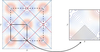
 η
η (x,y)
(x,y) x=±y
x=±y x+y=±L
 x−y=±L
 η
η (x,y)
(x,y) x=±y
x=±y
 η(x,y,T/4)
 (x,y)
(x,y) x=±y
x=±y x+y=±L
 x−y=±L
 x=±L1/2
 y=±L2/2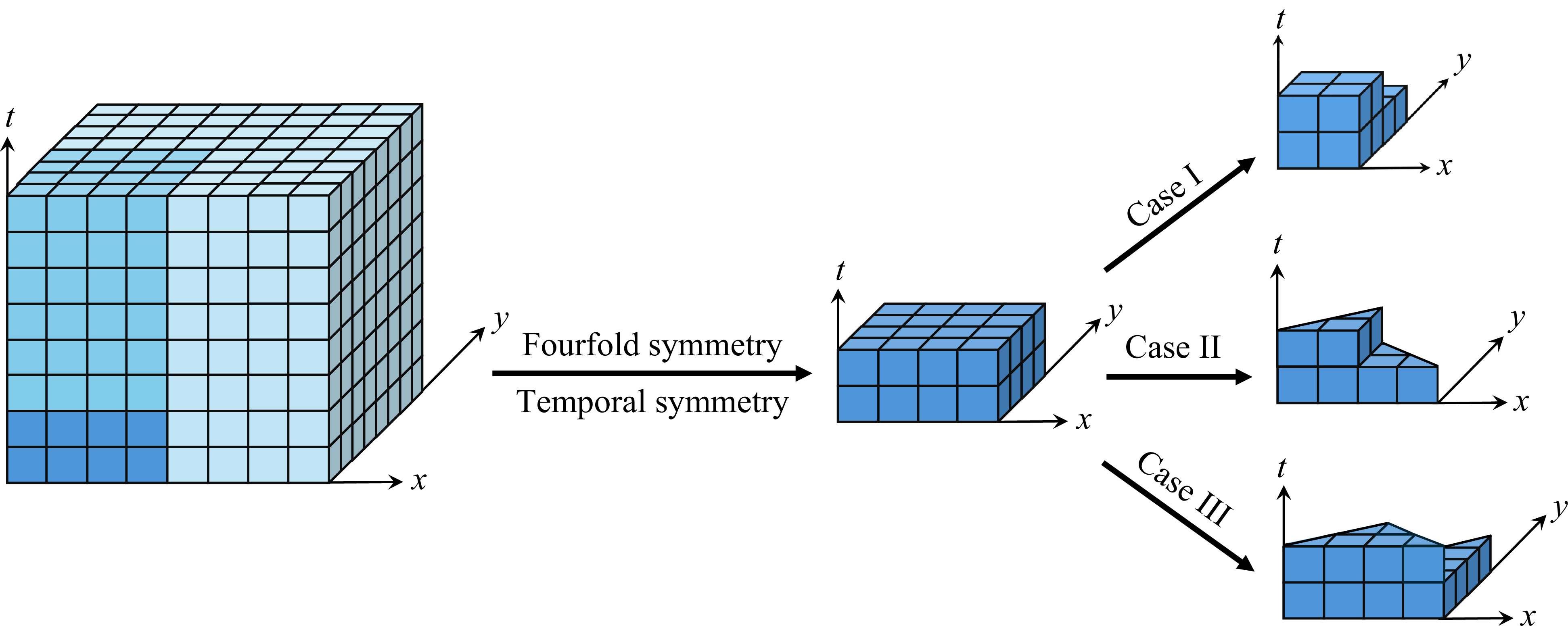

 k=1,h=∞
 ω
ω ϵ
ϵ 0.8
0.8 ϵ=0.394
 k=l=1,h=π
 ω
ω ϵ
ϵ H=0.46
 ϵ=0.3675
 k=l=1, H=0.7
 t=0,T/4,T/2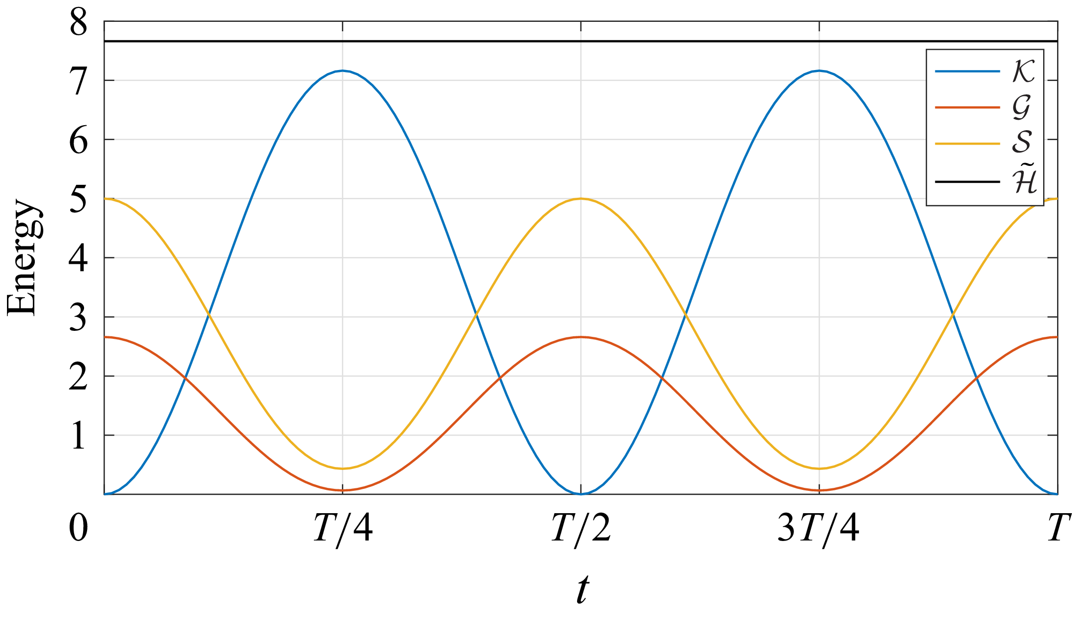
 K,G,S,H~
 H=0.1,0.2,0.4,0.6,0.7
 0.7cos(x)cos(y)
 k=l=1, H=0.33
 t=0,T/16,3T/16,7T/32,T/4
 100
100 η(x,y,0)
 t=0,T/32,T/16,…,T/4
 η(0,0,t)
 cos(pωt)
 p=0
p=0 p=20
p=20
 k=l=1
k=l=1
 k=1, l=0
 H=0.3
H=0.3 t=0,T/4,T/2
 H=0.29
 t=0
t=0
 α=β=1
α=β=1 α=−1, β=1
 κ
κ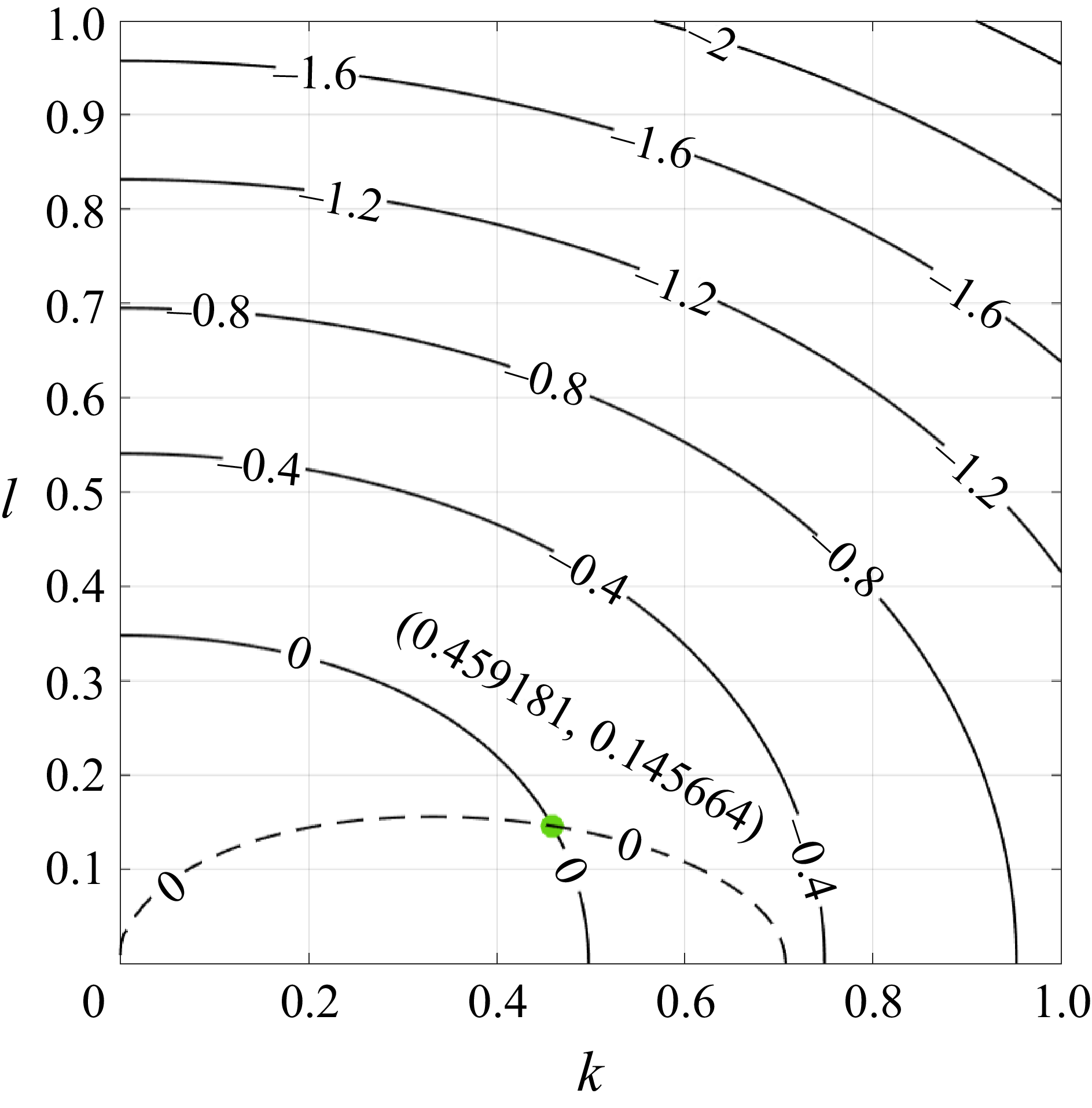
 α=2, β=4
 γ=2
γ=2 κ
κ
 k=l=0.5
 ω
ω H
H ϵ
ϵ
 k=l=0.5, H=0.73
 1
1 t=0,T/8,3T/16
 k=l=0.5, H=0.19
 2
2 t=0,T/8,3T/16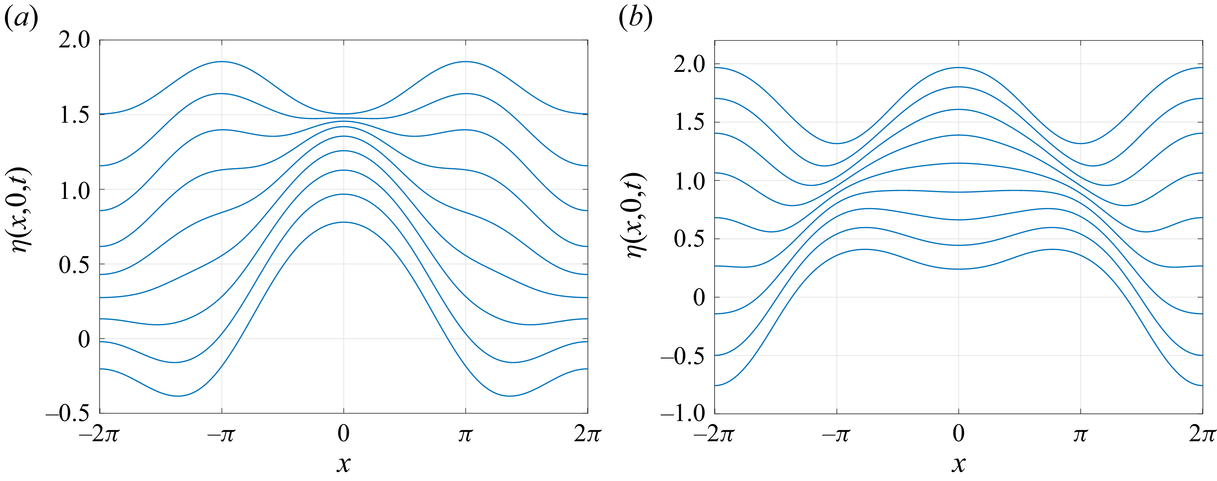
 y=0
y=0 1
1 H=0.73
 2
2 H=0.19
 t=0,T/32,T/16,…,T/4
 k=1, l=1.5312
 ω
ω H
H k=0, l=3.0624
 ϵ
ϵ ϵ
ϵ
 k=1
k=1 l=1.5312
 1
1 H=8×10⁻⁵
 H=10−3
 k=1, l=1.5312, H=0.4
 1
1 t=0,3T/16,T/4
 k=1, l=1.5312, H=0.135
 2
2 t=0,3T/16,T/4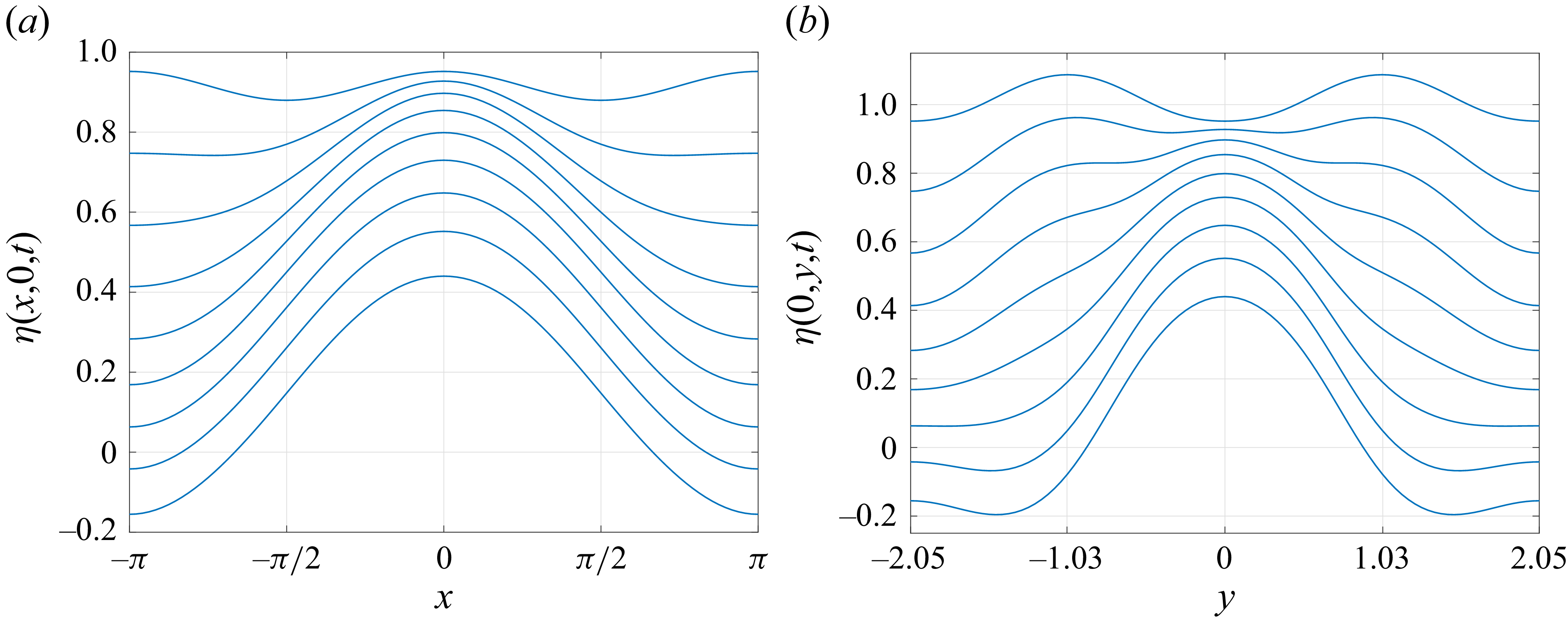
 y=0
y=0 1
1 H=0.4
H=0.4 x=0
x=0 t=0,T/32,T/16,…,T/4
 k=0.459181, l=0.145664
 ω
ω H
H ϵ
ϵ
 k=0.459181, l=0.145664
 t=0,T/8,T/4
 1
1 H=0.2
H=0.2 2
2 H=0.07
 3
3 H=0.195
 4
4 H=0.185
 x
x z
z
 η(0,0,t)
 k=l=1
k=l=1 k=l=0.5
 1
1 k=1, l=1.5312
 1
1 max(|φ(x,y,t/T)|)
 (k=l=1, H=0.29)
 0.001cos(x+y)
 |p^1,1|
 |p^−1,1|
 t=0,72T,137.1T,204.1T,273.2T
 (k=l=1, H=0.5)
 0.001cos(x+y)
 |p^1,1|
 |p^1,−1|
 t=26T
t=26T 61.6T
61.6T
 1
1 (k=1, l=1.5312, H=0.05)
 0.001cos(x+1.5312y)
 |p^1,1.5312|
 |p^1,−1.5312|
 |p^0,3.0624|
 t=0
t=0 453.2T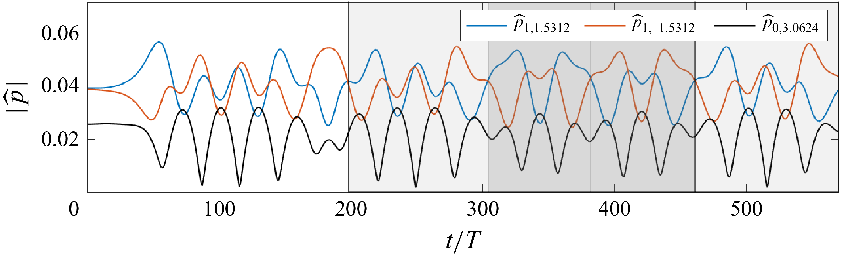
 |p^1,1.5312|
 |p^1,−1.5312|
 |p^0,3.0624|
 1
1 (k=1, l=1.5312, H=0.2)
 0.001cos(x+1.5312y)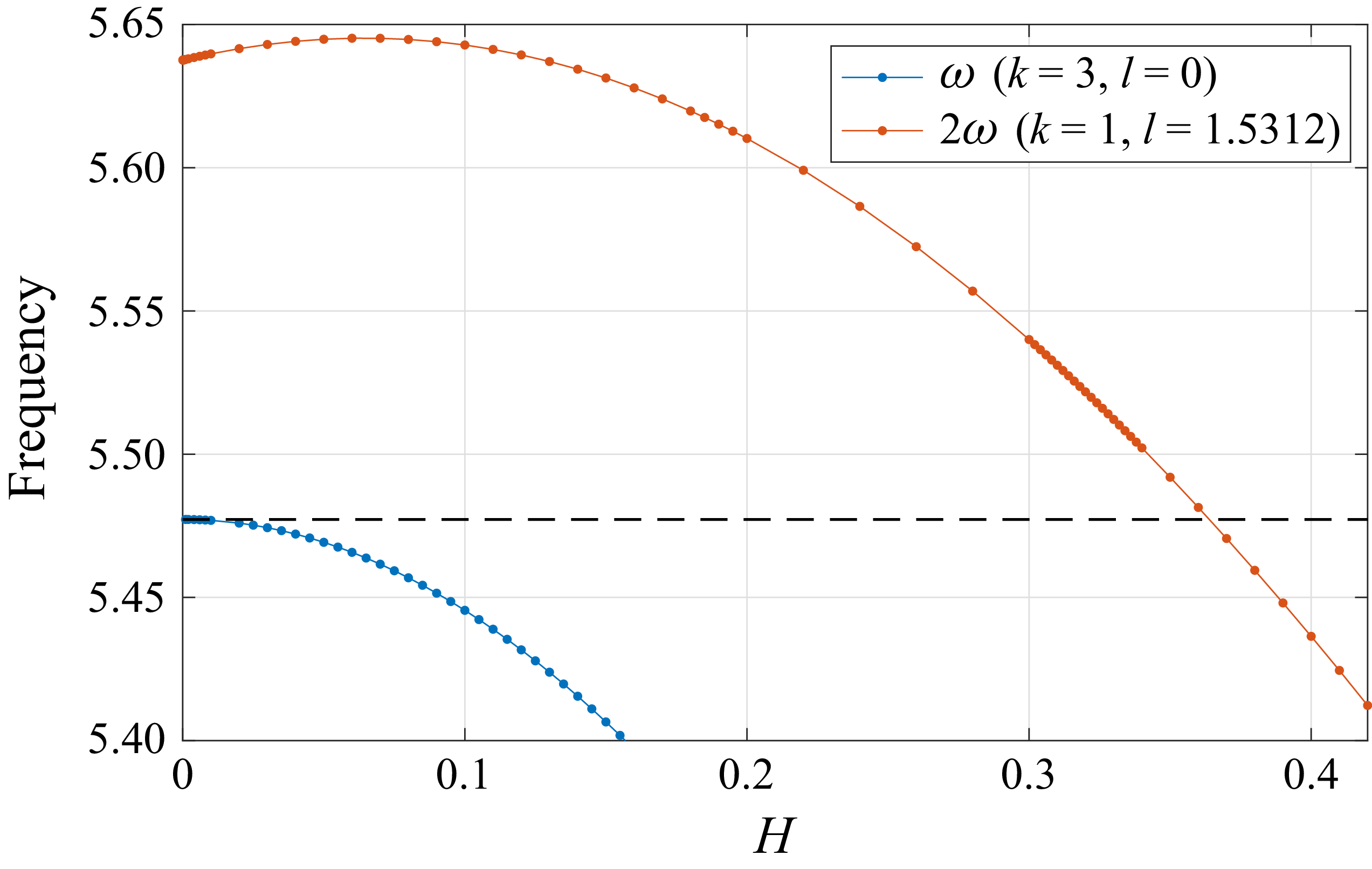
 1
1 k=1, l=1.5312
 k=3, l=0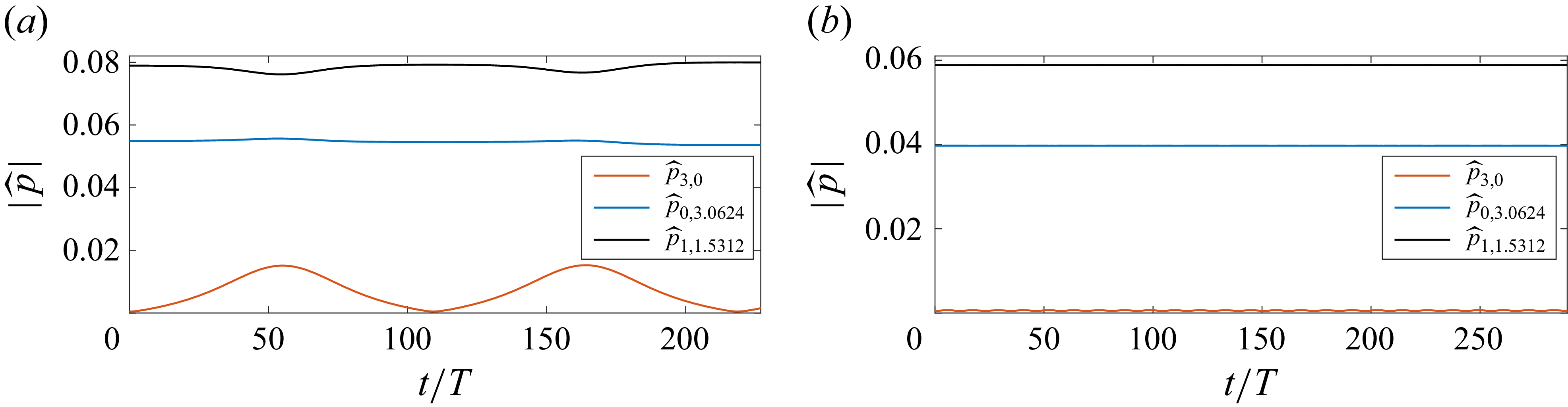
 |p^3,0|, |p^0,3.0624|, |p^1,1.5312|
 1
1 0.001cos(3x)
 H=0.4
H=0.4 H=0.3
H=0.3


 Open access

