


1. Introduction
In recent years, machine learning methods have been utilized to tackle various problems in fluid dynamics (Brenner, Eldredge & Freund Reference Brenner, Eldredge and Freund2019; Brunton, Hemanti & Taira Reference Brunton, Hemanti and Taira2020a; Fukami, Fukagata & Taira Reference Fukami, Fukagata and Taira2020a; Brunton, Noack & Koumoutsakos Reference Brunton, Noack and Koumoutsakos2020b). Applications of machine learning for turbulence modelling have been particularly active in fluid dynamics (Kutz Reference Kutz2017; Duraisamy, Iaccarino & Xiao Reference Duraisamy, Iaccarino and Xiao2019). Ling, Kurzawski & Templeton (Reference Ling, Kurzawski and Templeton2016) proposed a tensor-basis neural network based on the multilayer perceptron (known as MLP) (Rumelhart, Hinton & Williams Reference Rumelhart, Hinton and Williams1986) for Reynolds-averaged Navier–Stokes simulation. Embedding the Galilean invariance into the machine learning structure was found to be important and was verified by considering their model for flows in a duct and over a wavy wall. For large-eddy simulation, subgrid modelling assisted by machine learning was proposed by Maulik et al. (Reference Maulik, San, Rasheed and Vedula2019). They showed the capability of machine learning assisted subgrid modeling in a priori and a posteriori tests for the Kraichnan turbulence.
Furthermore, machine learning is proving itself as a promising tool for developing reduced-order models (ROMs). For instance, Murata, Fukami & Fukagata (Reference Murata, Fukami and Fukagata2020) proposed a nonlinear mode decomposition technique using an autoencoder (Hinton & Salakhutdinov Reference Hinton and Salakhutdinov2006) based on convolutional neural networks (CNN) (LeCun et al. Reference LeCun, Bottou, Bengio and Haffner1998) and demonstrated its use on transient and asymptotic laminar cylinder wakes at  $Re_D=100$. Their method shows the potential of autoencoder in terms of the feature extraction of flow fields in lower dimension. More recently, Hasegawa et al. (Reference Hasegawa, Fukami, Murata and Fukagata2020) combined a CNN and the long short-term memory (known as LSTM) (Hochreiter & Schmidhuber Reference Hochreiter and Schmidhuber1997) for developing an ROM for a two-dimensional unsteady wake behind various bluff bodies. Although the aforementioned examples deal with only laminar flows, the strengths of machine learning have been capitalized for ROM of turbulent flows. San & Maulik (Reference San and Maulik2018) utilized an extreme learning machine (Huang, Zhu & Siew Reference Huang, Zhu and Siew2004) based on multilayer perceptron for developing an ROM of geophysical turbulence. Srinivasan et al. (Reference Srinivasan, Guastoni, Azizpour, Schlatter and Vinuesa2019) used long short-term memory to predict temporal evolution of the coefficients of nine-equation turbulent shear flow model. They demonstrated that the chaotic behaviour of those coefficients can be reproduced well. They also confirmed that the statistics collected from machine learning agreed with the reference data.
Of particular interest here for fluid dynamics is the use of machine learning as a powerful approximator (Cybenko Reference Cybenko1989; Hornik Reference Hornik1991; Kreinovich Reference Kreinovich1991; Baral, Fuentes & Kreinovich Reference Baral, Fuentes and Kreinovich2018), which can handle nonlinearities. We recently proposed a super resolution (SR) reconstruction method for fluid flows, which was tested for two-dimensional laminar cylinder wake and two-dimensional decaying homogeneous isotropic turbulence (Fukami, Fukagata & Taira Reference Fukami, Fukagata and Taira2019a). We demonstrated that high-resolution two-dimensional turbulent flow fields of a  $128\times 128$ grid can be reconstructed from the input data on a coarse $4\times 4$ grid via machine learning methods. Applications and extensions of SR reconstruction can be considered for not only computational (Onishi, Sugiyama & Matsuda Reference Onishi, Sugiyama and Matsuda2019; Liu et al. Reference Liu, Tang, Huang and Lu2020) but also experimental fluid dynamics (Deng et al. Reference Deng, He, Liu and Kim2019; Morimoto, Fukami & Fukagata Reference Morimoto, Fukami and Fukagata2020). Although these attempts showed great potential of machine-learning-based SR methods to handle high-resolved fluid big data efficiently, their applicability has been so far limited only to two-dimensional spatial reconstruction.
In addition, the temporal data interpolation with various data-driven techniques has been used to process video images, including the optical flow-based interpolation (Ilg et al. Reference Ilg, Mayer, Saikia, Keuper, Dosovitskiy and Brox2017), phase-based interpolation (Meyer et al. Reference Meyer, Djelouah, McWilliams, Sorkine-Hornung, Gross and Schroers2018), pixels motion transformation (Jiang et al. Reference Jiang, Sun, Jampani, Yang, Learned-Miller and Kautz2018), and neural network-based interpolation (Xu et al. Reference Xu, Zhang, Wang, Belhumeur and Neumann2020). For instance, Li, Roblek & Tagliasacchi (Reference Li, Roblek and Tagliasacchi2019) developed a machine-learning-based temporal SR technique called inbetweening to estimate the snapshot sequences between the start and last frames for image and video processing. They generated 14 possible frames between two frames of videos using machine learning to save on storage. In the fluid dynamics community, a similar concept has recently been considered by Krishna et al. (Reference Krishna, Wang, Hemati and Luhar2020) to temporal data interpolation for PIV measurement. They developed a model based on the rapid distortion theory and Taylor's hypothesis.
In the present study, we perform a machine-learning-based spatio-temporal SR analysis inspired by the aforementioned spatial SR and temporal inbetweening techniques to reconstruct high-resolution turbulent flow data from extremely low-resolution flow data both in space and time. The present paper is organized as follows. We first introduce our machine-learning-based spatio-temporal SR approach in § 2 with a simple demonstration for a two-dimensional laminar cylinder wake at  $Re_D=100$. We then apply the present method to two-dimensional decaying isotropic turbulence and turbulent channel flow over a three-dimensional domain in § 3. The capability of a machine-learning-based spatio-temporal SR method is assessed statistically. Finally, concluding remarks are provided in § 4.
2. Approach
2.1. Spatio-temporal SR flow reconstruction with machine learning
The objective of this work is to reconstruct high-resolution flow field data  $\boldsymbol {q}(x_{HR}, t_{HR})$ from low-resolution data in space and time $\boldsymbol {q}(x_{LR}, t_{LR})$. To achieve this goal, we combine spatial SR analysis with temporal inbetweening. Super resolution analysis can reconstruct spatially high-resolution data from spatially input data, as illustrated in figure 1(a). Temporal inbetweening is able to find the temporal sequences between the first and the last frames in the time-series data, as shown in figure 1(b). We describe the methodology to combine these two reconstruction methods in § 2.1.
Data reconstruction methods used in the present study: (a) spatial SR; (b) temporal SR (inbetweening).

In the present study, we use a supervised machine learning model to reconstruct fluid flow data in space and time. For supervised machine learning, we prepare a set of input  $\boldsymbol {x}$ and output (answer) $\boldsymbol {y}$ as the training data. We then train the supervised machine learning model with these training data such that a nonlinear mapping function $\boldsymbol {y}\approx {\mathcal {F}}(\boldsymbol {x};\boldsymbol {w})$ can be built, where $\boldsymbol {w}$ holds weights within the machine learning model. The training process here can be mathematically regarded as an optimization problem to determine the weights ${\boldsymbol {w}}$ such that $\boldsymbol {w}=\textrm {argmin}_{\boldsymbol {w}}[{E}(\boldsymbol {y},{\mathcal {F}}(\boldsymbol {x};\boldsymbol {w}))]$, where $E$ is the loss (cost) function.
For the machine learning models for SR in space  $\mathcal {F}_x$ and time $\mathcal {F}_t$, we use a hybrid DSC/MS model (Fukami et al. Reference Fukami, Fukagata and Taira2019a) presented in figure 2. The DSC/MS model is based on a CNN (LeCun et al. Reference LeCun, Bottou, Bengio and Haffner1998) which is one of the widely used supervised machine learning methods for image processing. Here, let us briefly introduce the mathematical framework for the CNN. The CNN is trained with a filter operation such that
 \begin{equation} q^{(l)}_{ijm} = \varphi\left(b_m^{(l)}+\sum^{K-1}_{k=0}\sum^{H-1}_{p=0}\sum^{H-1}_{s=0}h_{p{s}km}^{(l)} q_{i+p-C,j+{s-C},k}^{(l-1)}\right), \end{equation}
where  $C={floor}(H/2)$, $b_m^{(l)}$ is the bias, $q^{(l)}$ is the output at layer $l$,
$l$,  $h$ is the filter, $K$ is the number of variables per each position of data and $\varphi$ is an activation function which is generally chosen to be a monotonically increasing nonlinear function. In the present paper, we use the rectified linear unit (known as ReLU), $\varphi (s) = {max}(0,s)$, as the activation function $\varphi$. It is widely known that the use of the rectified linear unit enables machine learning models to be stable during the weight update process (Nair & Hinton Reference Nair and Hinton2010).
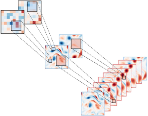
The hybrid downsampled skip-connection/multiscale (DSC/MS) SR model (Fukami et al. Reference Fukami, Fukagata and Taira2019a). Spatial reconstruction of two-dimensional cylinder wake at  $Re_D=100$ is shown as an example.

As shown in figure 2, the present machine learning model is comprised of two models: namely the DSC model shown in blue and the MS model shown in green. The DSC model is robust against rotation and translation of the objects within the input images by combining compression procedures and skip-connection structures (Le et al. Reference Le, Ngiam, Chen, Chia and Koh2010; He et al. Reference He, Zhang, Ren and Sun2016). On the other hand, the MS model (Du et al. Reference Du, Qu, He and Guo2018) is able to take the MS property of the flow field into account for its model structure. Readers are referred to Fukami et al. (Reference Fukami, Fukagata and Taira2019a) for additional details on the hybrid machine learning model. The DSC/MS model is utilized for both spatial and temporal data reconstruction in the present study. For the example of turbulent channel flow discussed in § 3.2, we use a three-dimensional convolution layer in place of the two-dimensional operations.
2.2. Order of spatio-temporal SR reconstruction
For the reconstruction of the flow field, we can consider the following two approaches.
(i) Apply the spatial SR model $\mathcal {F}_x^*:{\mathbb {R}}^{n_{LR}\times m_{LR}}\rightarrow {\mathbb {R}}^{n_{HR}\times m_{LR}}$, then the inbetweening model ${\mathcal {F}_t}:{\mathbb {R}}^{n_{HR}\times m_{LR}}\rightarrow {\mathbb {R}}^{n_{HR}\times m_\textrm {HR}}$ such that
(2.2)\begin{equation} \boldsymbol{q}(x_{HR}, t_{HR}) = \mathcal{F}_t(\mathcal{F}_x^*(\boldsymbol{q}(x_{LR}, t_{LR})))+\boldsymbol{\epsilon}_{tx}. \end{equation}
$\mathcal {F}_x^*:{\mathbb {R}}^{n_{LR}\times m_{LR}}\rightarrow {\mathbb {R}}^{n_{HR}\times m_{LR}}$, then the inbetweening model ${\mathcal {F}_t}:{\mathbb {R}}^{n_{HR}\times m_{LR}}\rightarrow {\mathbb {R}}^{n_{HR}\times m_\textrm {HR}}$ such that
(2.2)\begin{equation} \boldsymbol{q}(x_{HR}, t_{HR}) = \mathcal{F}_t(\mathcal{F}_x^*(\boldsymbol{q}(x_{LR}, t_{LR})))+\boldsymbol{\epsilon}_{tx}. \end{equation}(ii) Apply the inbetweening model
$\mathcal {F}_t^*:{\mathbb {R}}^{n_{LR}\times m_{LR}}\rightarrow {\mathbb {R}}^{n_{LR}\times m_{HR}}$, then the spatial SR model ${\mathcal {F}_x}:{\mathbb {R}}^{n_{LR}\times m_{HR}}\rightarrow {\mathbb {R}}^{n_{HR}\times m_{HR}}$ such that
(2.3)where\begin{equation} \boldsymbol{q}(x_{HR}, t_{HR}) = \mathcal{F}_x(\mathcal{F}_t^*(\boldsymbol{q}(x_{LR}, t_{LR})))+\boldsymbol{\epsilon}_{xt}, \end{equation}$n$ is a spatial dimension of data, $m$ is a temporal dimension of data, $\boldsymbol {\epsilon }_{tx}$ is the error for the first case and $\boldsymbol {\epsilon }_{xt}$ is the error for the second case. The subscripts LR and HR denote low-resolution and high-resolution variables, respectively.


We seek the approach that achieves the lower error between the above two formulations. The  $L_p$ norms of these error are assessed as
 \begin{align} ||\boldsymbol{\epsilon}_{tx}||_p &= ||\boldsymbol{q}(x_{HR},t_{HR})-\mathcal{F}_t(\mathcal{F}_x^*(\boldsymbol{q}(x_{LR},t_{LR})))||_p \nonumber\\ &= ||\boldsymbol{q}(x_{HR},t_{HR})-\mathcal{F}_t(\boldsymbol{q}(x_{HR},t_{LR})+\boldsymbol{\epsilon}_x)||_p, \end{align}
 \begin{align} ||\boldsymbol{\epsilon}_{xt}||_p &= ||\boldsymbol{q}(x_{HR},t_{HR})-\mathcal{F}_x(\mathcal{F}_t^*(\boldsymbol{q}(x_{LR},t_{LR})))||_p \nonumber\\ &= ||\boldsymbol{q}(x_{HR},t_{HR})-\mathcal{F}_x(\boldsymbol{q}(x_{LR},t_{HR})+\boldsymbol{\epsilon}_t)||_p, \end{align}
where  $\boldsymbol {\epsilon }_x$ is an error from the spatial SR algorithm for the first case and $\boldsymbol {\epsilon }_t$ is an error from the inbetweening process for the second case. Since the spatial SR algorithm is not a function of the temporal resolution algorithm in our problem setting, $\boldsymbol {\epsilon }_x$ is not affected much by the temporal coarseness of the given data. On the other hand, $\boldsymbol {\epsilon }_t$ is the error resulting from inbetweening with spatial low-resolution data which lacks the phase information compared with the spatially high-resolution data. For this reason, the error $\boldsymbol {\epsilon }_t$ is likely to be large due to the spatial coarseness. This leads us to first establish a machine learning model for spatio-temporal SR reconstruction as illustrated in figure 3 for the example of a cylinder wake. The cylinder flow example confirms the above error trend, as shown in figure 4. We also examine the possibility of utilizing a single combined model $\mathcal {F}_{comb}$, i.e. $\boldsymbol {q}(x_{HR}, t_{HR})=\mathcal {F}_{comb}(\boldsymbol {q}(x_{LR}, t_{LR}))$, which attempts to reconstruct the spatio-temporal high-resolution flow field from its counterpart directly. As presented in figure 4, the flow field cannot be reconstructed well. This is caused by the difficulty in weight updates while training the machine learning model. The observations here suggest that care should be taken in training machine learning models (Fukami, Nakamura & Fukagata Reference Fukami, Nakamura and Fukagata2020b).
Spatio-temporal SR reconstruction with machine learning for cylinder flow at  $Re_D = 100$.

Dependence of reconstruction performance on the order of training processes for cylinder flow. The first ( $t=1{\rm \Delta} t$), intermediate ( $t=5{\rm \Delta} t$) and last ( $t=9{\rm \Delta} t$) snapshots are shown. Reversed order refers to option (ii) in § 2.2. The combined model refers to $\mathcal {F}_{comb}$ which directly reconstructs $\boldsymbol {q}(x_{HR}, t_{HR})$ from $\boldsymbol {q}(x_{LR}, t_{LR})$. The values underneath the contours report the $L_2$ error norms.

Each of these machine learning models is trained individually for the spatial and temporal SR reconstructions. In the supervised machine learning process for regression tasks, the training process is formulated as an optimization problem to minimize a loss function in an iterative manner. The objectives of the two machine learning models can be expressed as
 \begin{align} \boldsymbol{w}_{x} = \textrm{argmin}_{\boldsymbol{w}_x} ||\boldsymbol{q}(x_{HR},t_{LR})-\mathcal{F}_x^*(\boldsymbol{q}(x_{LR},t_{LR}))||_p, \end{align}
 \begin{align}\boldsymbol{w}_{t} = \textrm{argmin}_{\boldsymbol{w}_t} ||\boldsymbol{q}(x_{HR},t_{HR})-\mathcal{F}_t(\boldsymbol{q}(x_{HR},t_{LR}))||_p, \end{align}
where  $\boldsymbol {w}_{x}$ and $\boldsymbol {w}_{t}$ are the weights of the spatial and temporal SR models, respectively. In the present study, we use the $L_2$ norm ( $\,{p}=2$) to determine the optimized weights $\boldsymbol {w}$ for each of the machine learning models. Hereafter, we use ${p}=2$ for assessing the errors.
2.3. Demonstration: two-dimensional laminar cylinder wake
For demonstration, let us apply the proposed formulation to the two-dimensional cylinder wake at  $Re_D=100$. The snapshots for this wake are generated by two-dimensional direct numerical simulation (DNS) (Taira & Colonius Reference Taira and Colonius2007; Colonius & Taira Reference Colonius and Taira2008), which numerically solves the incompressible Navier–Stokes equations,
 \begin{gather} \boldsymbol{\nabla} \boldsymbol{\cdot} \boldsymbol{u}= 0, \end{gather}
 \begin{gather}\frac{\partial \boldsymbol{u}}{\partial t}+\boldsymbol{u} \boldsymbol{\cdot} \boldsymbol{\nabla} \boldsymbol{u}=-\boldsymbol{\nabla} p+\frac{1}{Re_D}\nabla^2\boldsymbol{u}. \end{gather}
Here  $\boldsymbol {u}$ and $p$ are the non-dimensionalized velocity vector and pressure, respectively. All variables are made dimensionless by the fluid density $\rho$, the uniform velocity $U_\infty$ and the cylinder diameter $D$. The Reynolds number is defined as $Re_D=U_\infty D/\nu$ with $\nu$ being the kinematic viscosity. For this example, we use five nested levels of multidomains with the finest level being $(x, y)/D = [-1, 15] \times [-8, 18]$ and the largest domain being $(x,y)/D = [-5, 75] \times [-40, 40]$. Each domain uses $[N_x, N_y] = [400, 400]$ for discretization. The time step for DNS is set to ${\rm \Delta} t=2.50\times 10^{-3}$ and yields a maximum Courant–Friedrichs–Lewy number of 0.3. As the training data set, we extract the domain around a cylinder body over $(x^*,y^*)/D = [-0.7, 15] \times [-5, 5]$ with $(N_x,N_y) = (192, 112)$. For the present study, we use 70 % of the snapshots for training and the remaining 30 % for validation, which splits the whole data set randomly. The assessment of this demonstration is performed using 100 test snapshots excluding the training and validation data. Note here that the nature of training and test data sets are similar to each other due to the periodicity of the laminar two-dimensional circular cylinder wake. An early stopping criterion (Prechelt Reference Prechelt1998) with 20 iterations of the learning process is also utilized to avoid overfitting such that the model retains generality for any unseen data in the training process. For the input and output attributes to the machine learning model, we choose the vorticity field $\omega$.
The results from preliminary examination with the undersampled cylinder wake data are summarized in figure 5. The machine learning models are trained by using  $n_{{snapshot}, x}=1000$ for spatial SR and $n_{{snapshot}, t}=100$ for inbetweening. Both snapshots are prepared from a same time range which is approximately eight vortex shedding periods. Here, the spatial SR model $\mathcal {F}_x$ has the role of a mapping function from the low-spatial-resolution data $\boldsymbol {q}(x_{LR})\in {\mathbb {R}}^{12\times 7}$ to the high-spatial-resolution data $\boldsymbol {q}(x_{HR})\in {\mathbb {R}}^{192\times 112}$. Next, two spatial high-resolved flow fields illustrated only at $t=1{\rm \Delta} t$ and $9{\rm \Delta} t$ in figure 5 are used as the input for the temporal SR model $\mathcal {F}_t$, so that the in-between snapshots from $t=2{\rm \Delta} t$ to $8{\rm \Delta} t$ corresponding to a period in time can be reconstructed. As shown in figure 5, the spatio-temporal SR analysis achieves excellent reconstruction of the flow field that is practically indistinguishable from the reference DNS data. The $L_2$ error norm $\epsilon = ||{\omega }_{DNS}-{\omega }_{ML}||_2/||{\omega }_{DNS}||_2$ is shown in the middle of figure 5. The $L_2$ error level is approximately 5 % of the reference DNS data. As the machine learning model is provided with the information at $t = 1{\rm \Delta} t$ and $9 {\rm \Delta} t$, the error level shows slight increase between those two snapshots.
Spatio-temporal SR reconstruction with machine learning for cylinder wake at  $Re_D=100$. The bar graph located in the centre shows the $L_2$ error norm $\epsilon$ for the reconstructed flow fields. The contour level of the vorticity fields is same as that in figure 4.

3. Results
3.1. Example 1: two-dimensional decaying homogeneous isotropic turbulence
As the first example of turbulent flows, let us consider two-dimensional decaying homogeneous isotropic turbulence. The training data set is obtained by numerically solving the two-dimensional vorticity transport equation,
 \begin{equation} \frac{\partial \omega}{\partial t}+\boldsymbol{u}\boldsymbol{\cdot}\boldsymbol{\nabla}\omega= \frac{1}{Re_0}\nabla^2 \omega, \end{equation}
where  $\boldsymbol {u}=(u,v)$ and $\omega$ are the velocity and vorticity, respectively (Taira, Nair & Brunton Reference Taira, Nair and Brunton2016). The size of the biperiodic computational domain and the numbers of grid points here are $L_x=L_y=1$ and $N_x=N_y=128$, respectively. The Reynolds number is defined as $Re_0 \equiv u^*l_0^*/\nu$, where $u^*$ is the characteristic velocity obtained by the square root of the spatially averaged initial kinetic energy, $l_0^*=[2{\overline {u^2}}(t_0)/{\overline {\omega ^2}}(t_0)]^{1/2}$ is the initial integral length and $\nu$ is the kinematic viscosity. The initial Reynolds numbers are $Re_0 = u^*(t_0)l^*(t_0)/\nu =$ 81.2 for training/validation data and 85.4 for test data (Fukami et al. Reference Fukami, Fukagata and Taira2019a). For the input and output attributes to the machine learning model, we use the vorticity field $\omega$.
For spatio-temporal SR analysis of two-dimensional turbulence, we consider four cases comprised of two spatial and two temporal coarseness levels as shown in figure 6. For spatial SR analysis, we prepare two levels of spatial coarseness: medium- ( $16\times 16$) and low-resolution ( $8\times 8$ grids) data, analogous to our previous work (Fukami et al. Reference Fukami, Fukagata and Taira2019a). These spatial low-resolution data are obtained by an average downsampling of the reference DNS data set. Note that the reconstruction with SR for turbulent flows is influenced by the downsampling process, e.g. maximum or average values (Fukami et al. Reference Fukami, Fukagata and Taira2019a). We use the average pooling in the present work. For the temporal resolution set-up, we define a medium ( ${\rm \Delta} T=1.0$) and a wide time step ( ${\rm \Delta} T=4.0$), where ${\rm \Delta} T$ is the time step between the first and last frames of the inbetweening analysis. The decay of Taylor Reynolds number $Re_\lambda (t) = u^{\#}(t)\lambda (t)/\nu$, where $u^{\#}(t)$ is the spatial root mean square value for velocity at an instantaneous field and $\lambda (t)$ is the Taylor length scale at an instantaneous field, is shown in the middle of figure 6. The training data includes the low Taylor Reynolds number portion (regime II in figure 6) so as to assess the influence on the decaying physics compared with regime I. For the training process, we consider a fixed number of snapshots $(n_{{snapshot}, x},n_{{snapshot}, t})=(10\,000,10\,000)$ for all four cases of this two-dimensional example. The models for the considered four cases are constructed separately.
The problem set-up of spatio-temporal SR analysis for two-dimensional decaying homogeneous isotropic turbulence. The curve located in the centre is the decay of Taylor Reynolds number  $Re_{\lambda }$. The vorticity fields $\omega$ at the time stamps (a)–(f) along this curve are shown on the right-hand side.

For the example of two-dimensional turbulence, the machine learning model for inbetweening analysis plays the role of a regression function to reconstruct eight snapshots between the first and last frames (given by the spatial reconstruction model). The flow fields reconstructed from spatio-temporal SR analysis of two-dimensional turbulence with various coarse input data are summarized in figure 7. On the left-hand side, the reconstructed fields from regime I with coarse spatio-temporal data are shown. As can be seen, the temporal evolution of the complex vortex dynamics can be accurately reconstructed by the machine-learned models. For almost all cases, the  $L_2$ error norms $\epsilon = ||\boldsymbol {q}_{DNS}-\boldsymbol {q}_{ML}||_2/||\boldsymbol {q}_\textrm {DNS}||_2$ listed below the contour plots for the spatially low-resolution input show larger errors compared with the medium-resolution case due to the effect of input spatial coarseness. On the right-hand side of the figure, we show the results from regime II. Analogous to the results for regime I, the reconstructed flow fields are in agreement with the reference DNS data. Noteworthy here is the peak $L_2$ error norm of 0.198 appearing at $t=(n+7){\rm \Delta} t$ for regime II using low-resolution input and a wide time step. This is in contrast with the other cases that give peak errors at $t=(n+4){\rm \Delta} t$. This is likely because the present machine learning model, which does not embed information of boundary condition, has to handle the temporal evolution of a relatively large structure over a biperiodic domain (i.e. bottom left on the colourmap). Furthermore, the model is also affected by the error from the spatial SR reconstruction. For these reasons, the peak in error is shifted in time compared with the other cases in figure 7.
Spatio-temporal SR reconstruction for two-dimensional decaying homogeneous turbulence. The vorticity field  $\omega$ is shown with the same contour level in figure 6. Medium- and low-resolution spatial input with (a) medium time step for regime I, (b) medium time step for regime II, (c) wide time step for regime I and (d) wide time step for regime II. The values underneath the flow fields report the $L_2$ error norms.

To examine the dependence on the regime of test data, the time-ensemble  $L_2$ error norms of medium- and low-spatial-input cases are shown in figure 8. For all cases, the errors for regime I are larger than those for regime II. One of reasons here is that the relative change in vortex structures for regime II is less than that for regime I, which we can see in figure 7. We also find that the reconstructions are affected by the input coarseness in space as evident from comparing figures 8(a) and 8(b). Similar trends can also be seen in figure 9 which show the total kinetic energy $E_{tot}$ over the domain for each case. The curves shown here do not decrease monotonically since we take the ensemble average over the test data, whose trend is analogous to the decay of Taylor Reynolds number as presented in figure 6. By comparing figures 7 and 9, it is inferred that the present machine learning model can capture the decaying nature of two-dimensional turbulence.
Time-ensemble  $L_2$ error norms for the (a) medium- and (b) low-spatial-input cases.

Decay of time-ensemble total kinetic energy  $E_{tot}$ over the domain.

Next, let us present the kinetic energy spectrum and the p.d.f. of the vorticity field  $\omega$ for all coarse input cases with spatio-temporal reconstructions in figure 10. For comparison, we compute these statistics for regimes I (purple) and II (yellow). The statistics with all coarse input data show similar distributions with the reference DNS trends. The high-wavenumber region of the kinetic energy spectrum obtained from the reconstructed fields do not match with the reference curve due to the lack of correlation between the low- and high-wavenumber components. Through our investigation in this section, we can exemplify that the present machine learning model can successfully work in reconstructing high-resolution two-dimensional turbulence from spatio-temporal low-resolution data.
Statistical assessments for the spatio-temporal SR analysis of two-dimensional turbulence. (a,c,e,g) Kinetic energy spectrum; (b,d,f,h) probability density function (p.d.f.) of vorticity  $\omega$; (a–d) medium time step; (e–h) wide time step; (a,b,e,f) regime I; (c,d,g,h) regime II.

3.2. Example 2: turbulent channel flow over three-dimensional domain
To investigate the applicability of machine-learning-based spatio-temporal SR reconstruction to three-dimensional turbulence, let us consider a turbulent channel flow (Fukagata, Kasagi & Koumoutsakos Reference Fukagata, Kasagi and Koumoutsakos2006). The governing equations are the incompressible Navier–Stokes equations,
 \begin{gather} {\boldsymbol{\nabla}} \boldsymbol{\cdot} \boldsymbol{u} = 0, \end{gather}
 \begin{gather}{\dfrac{\partial \boldsymbol{u}}{\partial t} + {\boldsymbol{\nabla}} \boldsymbol{\cdot} (\boldsymbol{uu}) = -{\boldsymbol{\nabla}} p + \dfrac{1}{{Re}_\tau}\nabla^2 \boldsymbol{u}}, \end{gather}
where  ${\boldsymbol {u}} = [u\ v\ w]^{\mathrm {T}}$ represents the velocity vector with components $u$,
$u$,  $v$ and $w$ in the streamwise ( $x$), wall-normal ( $y$) and spanwise ( $z$) directions. Here, $t$ is time, $p$ is pressure and ${{Re}_\tau = u_\tau \delta /\nu }$ is the friction Reynolds number. The variables are normalized by the half-width $\delta$ of the channel and the friction velocity $u_\tau =(\nu \,{\textrm {d}U}/{\textrm {d} y}|_{y=0})^{1/2}$, where $U$ is the mean velocity. The size of the computational domain and the number of grid points here are $(L_{x}, L_{y}, L_{z}) = (4{\rm \pi} \delta , 2\delta , 2{\rm \pi} \delta )$ and $(N_{x}, N_{y}, N_{z}) = (256, 96, 256)$, respectively. The grids in the $x$ and $z$ directions are taken to be uniform. A non-uniform grid is utilized in the $y$ direction with stretching based on the hyperbolic tangent function.
As the baseline data, we prepare the data snapshots on a uniform grid interpolated from the non-uniform grid data of DNS. The influence of grid type is reported in the Appendix for completeness. The no-slip boundary condition is imposed on the walls and a periodic boundary condition is prescribed in the  $x$ and $z$ directions. The flow is driven by a constant pressure gradient at ${Re}_{\tau }=180$. For the present study, a subspace of the whole computational domain is extracted and used for the training process, i.e. $(L_x^*,L_y^*,L_z^*)=(2{\rm \pi} \delta ,\delta ,{\rm \pi} \delta )$, $x, y, z \in [0,L_x^*] \times [0,L_y^*] \times [0,L_z^*]$, and $(N_{x}^*, N_{y}^*, N_{z}^*) = (128, 48, 128)$. Due to the symmetry of turbulence statistics in the $y$ direction and homogeneity in the $x$ and $z$ directions, the extracted subdomain maintains the turbulent characteristics of the channel flow over the original domain size. We generally use 100 training data sets for both the spatial and temporal SR analyses in this case. The dependence of the reconstruction on the number of snapshots is investigated later. For all assessments in this example, we use 200 test snapshots excluding the training data. For the input and output attributes to the machine learning model, we use the velocity fields ${\boldsymbol {u} = [u\ v\ w]^{\mathrm {T}}}$. Hereafter, the superscript $+$ is used to denote quantities in wall units.
We illustrate in figure 11 the problem setting of the spatio-temporal SR analysis for three-dimensional turbulence. For visualization here, we use the second invariant of the velocity gradient tensor  $Q$. Regarding the spatial resolution, medium and low resolutions are defined as $16\times 6\times 16$ and $8\times 3\times 8$ grids in the $x$,
$x$,  $y$ and $z$ directions, respectively. These coarse input data sets are generated by the average downsampling operation from the reference DNS data of $128\times 48\times 128$ grids. Note that we are unable to detect the vortex core structures at $Q^+=0.005$ with low-resolution input in figure 11 due to the gross coarseness. As shown in figure 12, the vortex structure cannot be seen with a contour level of $Q^+=0.07$ with either medium- or low-spatial-input data. For the inbetweening reconstruction, three time steps are considered; ${\rm \Delta} T^+=12.6$ (medium), 25.2 (wide) and 126 (superwide time step) in viscous time units, where ${\rm \Delta} T^+$ is the time step between first and last snapshots. These ${\rm \Delta} T^+$ correspond to temporal two-point correlation coefficients at $y^+=11.8$ of $\mathcal {R}=R^+_{uu}(t^+)/R^+_{uu}(0)\approx 0.50$ (medium), 0.25 (wide) and 0.05 (superwide time step), where $R^+_{uu}(t^+; y^+) = \overline {u^{\prime +}(x^+, y^+, z^+, \tau ^+) u^{\prime +} (x^+, y^+, z^+, \tau ^+ - t^+)}^{x^+,z^+,\tau ^+}$, $\bar {\cdot }^{x^+,z^+,\tau ^+}$ denotes the time-ensemble average over the $x\text {--}z$ plane, and $u^\prime$ is the fluctuation of streamwise velocity (Fukami et al. Reference Fukami, Nabae, Kawai and Fukagata2019b).
The problem set-up for example 2. We consider two spatial coarseness levels with three temporal resolutions. Note that  $Q^+=0.005$ and 0.07 are used for visualization of spatial and temporal resolutions, respectively. The plot on the upper right-hand side shows the temporal two-point correlation coefficients $\mathcal {R}$ at $y^+=11.8$ for the present turbulent channel flow.

Isosurfaces of the  $Q$ criterion ( $Q^+=0.07$). (a) The input coarse data with medium and low resolutions. For comparison, $Q^+=0.005$ with medium-resolution is also shown. (b) Reference DNS data. (c) Reconstructed flow field from medium-resolution input data. (d) Reconstructed flow field from low-resolution input data.

Let us summarize the reconstructed flow field visualized by the  $Q$-criteria isosurface based on $n_{{snapshots},x}=100$ in figure 12. The machine learning models are able to reconstruct the flow field from extremely coarse input data, despite the input data showing almost no vortex-core structures in the streamwise direction as shown in figure 12(a). We also present the velocity contours at a $y$–
$y$– $z$ section ( $x^+=1127$) in figure 13. We report the $L_2$ error norms normalized by the fluctuation component $\epsilon = ||{u}_{i,DNS}-{u}_{i,ML}||_2/||{u}^\prime _{i,DNS}||_2$ in this example to remove the influence on magnitude of each velocity attribute in the present turbulent channel flow. With both coarse input data, the reconstructed flow fields are in reasonable agreement with the reference DNS data in terms of the contour plots and the $L_2$ error norms listed below the reconstructed flow field. We also assess the turbulence statistics as summarized in figure 14. Noteworthy here are the trends in the wall-normal direction that are well captured by the machine learning model from as little as six (medium-) or three (low-resolution) grid points, as shown in figures 14(a) and 14(b). Regarding the kinetic energy spectrum at $y^+=11.8$, the maximum wavenumber $k_{max}$ in the streamwise and spanwise directions can also be recovered from the extremely coarse input data as presented in figures 14(c) and 14(d). The high-wavenumber components for both cases show differences due to the fact that the dissipation range has no strong correlation with the energy-containing region. The aforementioned observation for the kinetic energy spectrum is distinct from that of two-dimensional turbulence. The under or overestimation of the kinetic turbulent energy spectrum here is likely caused by a combination of several reasons, e.g. underestimation of $u$ because of the $L_2$ regression and relationship between a squared velocity and energy such that $\overline {u^2} = \int E^+_{uu}(k^+) \,\textrm {d}k^+$. Whether machine-learning-based approaches consistently yield underestimated or overestimated kinetic energy spectrum likely depends on the flow of interest. While the overall method aims to minimize the loss function in the derivation, there are no constraints imposed for optimizing the energy spectrum in the current approach.
Velocity contours at a  $y\text{--}z$ section ( $x^+=1127$) of the reference DNS data, coarse input data and the recovered flow field through spatial SR analysis with machine learning (ML). The values listed below the contours are the $L_2$ error norm $\epsilon$.

Turbulence statistics of the reference DNS data, medium resolution (MR) input, low resolution (LR) input, and recovered flow fields by spatial SR analysis. (a) Root mean square of velocity fluctuation  $u_{i,{\textit{rms}}}$, (b) Reynolds stress $-u^\prime v^\prime$, (c) streamwise energy spectrum $E^+_{uu}(k_x^+)$ and (d) spanwise energy spectrum $E^+_{uu}(k_z^+)$.

Next, let us combine the spatial SR reconstruction with inbetweening to obtain the spatio-temporal high-resolution data  $\boldsymbol {q}(x_{HR},t_{HR})$, as summarized in figure 15. We only show in figure 15(a) the results for the medium-spatial-resolution input. With the medium time step, the reconstructed flow fields show reasonable agreement with the reference DNS data in terms of both the $Q$ isosurface and $L_2$ error norm listed below the isosurface plots. In contrast, the flow fields cannot be reconstructed with wide and superwide time steps due to the lack of temporal correlation, as summarized in figure 11. Although the vortex core can be somewhat captured with the wide time step at $n+2$ and $n+7$, the reconstructed flow fields are essentially smoothed since the machine-learned models for inbetweening are given only the information with low correlation at the first and last frames obtained from spatial SR reconstruction, as shown in figure 15(b). The time-ensemble $L_2$ error norm $\bar {\epsilon }$ with all combinations of coarse input data in space and time are summarized in figure 15(c). It can be seen that the results with the machine-learned models are more sensitive to the temporal resolution than the spatial resolution level. This observation agrees with the previous example in § 3.1.
Spatio-temporal SR reconstruction of turbulent channel flow over three-dimensional domain. (a) The  $Q$ isosurfaces ( $Q^+=0.07$) of the reference DNS and super-resolved flow field with medium, wide and superwide time step. The medium-resolution data in space are used as the input for spatial SR reconstruction. (b) The $L_2$ error norm of inbetweening for spatial medium-resolution input with wide time step. (c) Summary of the time-ensemble $L_2$ error norms for all combinations of coarse input data in space and time.

Let us demonstrate the robustness of the composite model against noisy input data for spatio-temporal SR analysis in figure 16. For this example, we use the medium spatially coarse input data with the medium time step. Here, the  $L_2$ error norm for noisy input is defined as $\epsilon ^\prime _{noise} = ||\boldsymbol {q}_{HR}-\mathcal {F}(\boldsymbol {q}_{LR}+\kappa \boldsymbol {n})||_2/||\boldsymbol {q}^{\prime }_{HR}||_2$, where $\boldsymbol {n}$ is the Gaussian noise for which the mean of the distribution is the value on each grid point and the standard deviation scale is 1, $\kappa$ is the magnitude of noisy input, and $\boldsymbol {q}^{\prime }_{HR}$ is the fluctuation component of the reference velocity. The reported values on the right-hand side of figure 16 are the ensemble-averaged $L_2$ error ratio against the original error without noisy input, $\overline {\epsilon ^\prime }/\overline {\epsilon ^\prime _{\kappa =0}}$. As shown, the error increases with the magnitude of noise $\kappa$ for both coarse input levels. The $x$–
$x$– $z$ sectional streamwise velocity contours from intermediate output of inbetweening at $t=(n+5){\rm \Delta} t$ are shown in the left-hand side of figure 16. The model exhibits reasonable robustness for the considered noise levels, especially for reconstructing large-scale structures.
Robustness of the machine learning model for noisy input with medium time step models. The  $x$–
$x$– $z$ sectional streamwise velocity contours are chosen from $y^+=19.4$, with medium-spatial-coarse input model. The contour plots visualize the intermediate snapshots at $t=(n+5){\rm \Delta} t$ for each noise level.

In the above discussions, we used 100 snapshots for both spatial and temporal SR analyses with three-dimensional turbulent flow. Here, let us discuss the dependence of the results on the number of snapshots for the spatial SR analysis  $n_{{snapshot,}x}$ and inbetweening $n_{{snapshot,}t}$. The ensemble $L_2$ error norm $\bar {\epsilon }$ with various number of snapshots is presented in figure 17. We summarize in this figure the effect from the number of training snapshots on the spatial and temporal reconstructions. Up to $n_{{snapshot},t}=50$, the $L_2$ errors are approximately 0.4 and the reconstructed fields cannot detect vortical structures from the $Q$-value visualizations, even if $n_{{snapshot,}x}$ is increased. For cases with $n_{{snapshot,}t}\geqslant 100$ and $n_{{snapshot,}x}\geqslant 100$, the errors drastically decrease. For this particular example with the turbulent channel flow, 100 training data sets is the minimum requirement for recovering the flow field for both in space and time. These findings suggest that data sets consisting with as few as 100 snapshots with the appropriate spatial and temporal resolutions hold sufficient physical characteristics for reconstructing the turbulent channel flow at this Reynolds number.
Influence of the number of the training snapshots for spatial SR reconstruction  $n_{{snapshot,}x}$ on the ensemble $L_2$ error norm $\bar {\epsilon }$.

Next, we assess the computational costs with increasing number of training data sets for the NVIDIA Tesla V100 graphics processing unit (known as GPU), as shown in figure 18. The computational time per an iteration (epoch) linearly increases with the number of snapshots for both spatial and temporal SR analyses. Plainly speaking, complete training process takes approximately three days with  $\{n_{{snapshot},x},n_{{snapshot},t}\}=\{100,100\}$ and 15 days with $\{n_{{snapshot},x},n_{{snapshot},t}\}=\{1000,1000\}$. The computational costs for the full iterations can deviate slightly from the linear trend since the error convergence is influenced within the machine learning models due to early stopping.
Influence of the number of snapshots on the computational time per epoch (axis on the left-hand side) and total computational time (axis on the right-hand side).

Let us also discuss the challenges associated with the spatio-temporal machine-learning-based SR reconstruction. As discussed above, a supervised machine learning model is trained to minimize a chosen loss function through an iterative training process. In other words, the machine learning models aim to solely minimize the given loss function, which is different from actually learning the physics. We here discuss the dependence of the error in the real space and wave space.
The  $L_2$ error distribution over each direction of turbulent channel flow is summarized in figure 19. The case with combination of medium-spatial-input ( $16\times 6 \times 16$ grids) with medium time step ( ${\rm \Delta} T^+=12.6$) is presented. As shown in figure 19, the errors at the edge of the domain in all directions are large. This is likely due to the difficulty in predicting the temporal evolution over boundaries and the padding operation of CNN. Noteworthy here is the error trend in the wall-normal direction in figure 19(c). The errors for all attributes are high near the wall. One of possible reasons is the low probability of velocity attributes near wall region, i.e. high flatness factor (Kim, Moin & Moser Reference Kim, Moin and Moser1987). Since the present machine learning models are trained with $L_2$ minimization as mentioned above, it is tougher to predict those region than high probability for fluctuations.
Dependence of  $L_2$ error norm $\epsilon$ on location of turbulent channel flow in the (a) streamwise ( $x$), (b) spanwise ( $z$) and (c) wall-normal ( $y$) directions. For clarity, a log-scale is used for panel (c).

We further examine how well the machine learning model performs over the wavenumber space. The kinetic energy spectrum at  $y^+=11.8$ in the streamwise and spanwise directions of spatio-temporal SR reconstruction are shown in figure 20. For the input data, spatial medium-resolution ( $16\times 6\times 16$ grids) with medium ( ${\rm \Delta} T^+=12.6$) and wide time steps ( ${\rm \Delta} T^+=25.2$) are considered. The $L_2$ error here is defined as $\epsilon _{E^+_{uu}}(t^+)=||E^+_{uu}(t^+)_{DNS}-E^+_{uu}(t^+)_{ML}||_2/||E^+_{uu}(t^+)_{DNS}||_2$. With the medium time step, the error over the high-wavenumber space are higher than that over the low-wavenumber space. This observation agrees with the machine learning models being able to recover the low-wavenumber space from grossly coarse data seen in figure 14. With the use of wide time step, we can infer the influence of temporal coarseness, as discussed above. The $L_2$ error distributions of kinetic energy spectrum show high-error concentration on high-wavenumber portion at intermediate output in time, as shown in the bottom part of figure 20. The machine learning models capture low-wavenumber components preferentially to minimize the reconstruction error.
Streamwise and spanwise kinetic energy spectrum of spatio-temporal SR analysis. Top results are based on medium time step and bottom results are based on wide time step. The left-hand side presents the streamwise energy spectrum and the right-hand side shows the spanwise energy spectrum.

4. Conclusions
We developed supervised machine learning methods for spatio-temporal SR analysis to reconstruct high-resolution flow data from grossly under-resolved input data both in space and time. First, a two-dimensional cylinder wake was considered as a demonstration. The machine-learned model was able to recover the data in space and reconstruct the temporal evolution from only the first and last frames.
As the first turbulent flow example, a two-dimensional decaying homogeneous isotropic turbulence was considered. In this example, we considered two spatial resolutions based on our previous work (Fukami et al. Reference Fukami, Fukagata and Taira2019a) and two different time steps to examine the capability of the proposed model. The reconstructed flow fields were in reasonable agreement with the reference data in terms of the  $L_2$ error norm, the kinetic energy spectrum, and the p.d.f. of vorticity field. We also found that the machine-learned models were affected substantially by the temporal range of training data.
We further examined the capability of the proposed method using a turbulent channel flow over three-dimensional domain at  $Re_\tau =180$. The machine-learning-based spatio-temporal SR analysis showed its great capability to reconstruct the flow field from grossly coarse input data in space and time when an appropriate time step size between the first and the last frames is used. The proposed method, however, was unable to recover the turbulent flow fields in time when the temporal two-point correlation coefficient was $\mathcal {R}^+\leqslant 0.25$. It was also seen that the machine learning models tend to preferentially extract the features in the low-wavenumber space so as to minimize a loss function efficiently. For improving the accuracy of the spatio-temporal SR analysis, we likely need to prepare a well-designed architecture which can take physics into account in its structure, e.g. loss function (Lee & You Reference Lee and You2019; Maulik et al. Reference Maulik, Fukami, Ramachandra, Fukagata and Taira2020; Raissi, Yazdani & Karniadakis Reference Raissi, Yazdani and Karniadakis2020) and choice for input and output attributes, i.e. feature engineering. In addition, care should also be taken for the proper choice of training data set which highly relates to the remaining problem – the distinction of interpolation and extrapolation for training data is still vague (Taira Reference Taira2019). Such efforts will be undertaken in future work.
The robustness of the present model for noisy input and dependence on the number of training snapshots were also investigated. The proposed model showed reasonable capability for up to  $10\,\%$ noisy input in terms of both qualitative and quantitative assessments. We found that the flow field can be reconstructed by the machine-learning-based methods with as few as 100 training data sets for both the spatial and temporal models.
We foresee a range of applications for the spatio-temporal super resolution analysis in fluid dynamics. For example, we may be able to leverage the current technique for large-eddy simulations as an augmentation tool. We may also be able to consider SR as a data compression tool to store big data, which will also makes it easier to share or exchange spatio-temporal data of complex flows among researchers. In fact, in the present paper, we can recover the three-dimensional turbulent channel flow field comprised of 7.9 million spatio-temporal elements from low-resolution data which have only 3072 spatio-temporal elements. This translates to a significant compression of  $0.04\,\%$.
The ability to reconstruct turbulent flow fields from a small number of data points in space and time has the potential for novel data compression techniques using machine learning models. However, the success of flow field reconstruction hinges on developing an appropriate neural network construct that accommodates the complex nonlinear physics of turbulence. When successful, the neural networks are able to condense the flow field to its skeleton giving hope for autoencoder-based approaches to identify the suitable coordinates to represent the primary axes of turbulent flow data in a nonlinear sense (Fukami et al. Reference Fukami, Nakamura and Fukagata2020b).
Acknowledgements
K.F. and K.F. thank the Japan Society for the Promotion of Science (KAKENHI grant number: 18H03758) for their support. K.T. acknowledges the generous support from the US Army Research Office (grant number: W911NF-17-1-0118) and the US Air Force Office of Scientific Research (grant number: FA9550-16-1-0650). K.F. also thanks T. Murata, M. Morimoto, T. Nakamura (Keio Univ.) and K. Hasegawa (Keio Univ., Polimi) for insightful discussions.
Declaration of interests
The authors report no conflict of interest.
Appendix
In this Appendix, we assess the influence of spatial discretizations in the wall-normal direction on the results from filter operation of the CNN. These operations are generally performed on uniform resolution image data. Note that we use the interpolated flow fields on a uniform grid generated from the non-uniform grid data in the  $y$ direction, as input and output attributes for the discussions in the main text.
Here, we do not interpolate but instead use the data on a non-uniform grid. We present the streamwise velocity contours at a  $y$–
$y$– $z$ section of spatial SR analysis with medium coarseness input data for both grid types in figure 21(a). Although we observe some visual differences in the input data as shown in figure 21(a), significant differences are not observed in terms of the streamwise velocity contours and the $L_2$ error norm. We also compare the $L_2$ error norm of the spatio-temporal SR analysis with both grid types in figure 21(b). For all cases, the errors using the uniform grid data are slightly larger than those from the non-uniform grid data. This is due to the original non-uniform data holding more information in the near-wall region compared with the uniform grid data. However, the filter operation of the CNN is not sensitive to the choice of the spatial discretization, at least for this problem.
(a) Dependence on the grid style of streamwise velocity contours  $u$ at a $y$–
$y$– $z$ section ( $x^+=1127$) for spatial SR reconstruction with machine learning (ML). Listed values are $L_2$ error norm. (b) Time-ensemble $L_2$ error norm of spatio-temporal SR reconstruction with uniform and non-uniform grid data in wall-normal direction.


 Open access