


1. Introduction
Boundary layers in practical engineering applications rarely develop under ideal zero-pressure-gradient conditions. Flows over hulls, fuselages and swept wings are strongly influenced by pressure gradients and curvature of the mean streamlines. Past studies have demonstrated the importance of these effects on the development of boundary layers and the state of turbulence (Mager Reference Mager1951; Cooke Reference Cooke1958; Bradshaw & Young Reference Bradshaw and Young1973; Finnigan Reference Finnigan1983). The flow around the canonical $6 \colon\! 1$
prolate spheroid highlights the complexity of these phenomena, with interacting streamwise, crossflow and centrifugal instabilities contributing to transition. The spheroid geometry has been studied experimentally (Fu et al. Reference Fu, Shekarriz, Katz and Huang1994; Chesnakas & Simpson Reference Chesnakas and Simpson1994, Reference Chesnakas and Simpson1996, Reference Chesnakas and Simpson1997; Wetzel Reference Wetzel1996) and numerically (Hedin et al. Reference Hedin, Berglund, Alin and Fureby2001; Constantinescu et al. Reference Constantinescu, Pasinato, Wang, Forsythe and Squires2002; Xiao et al. Reference Xiao, Zhang, Huang, Chen and Fu2007; Fureby & Karlsson Reference Fureby and Karlsson2009; Aram et al. Reference Aram, Shan and Jiang2021, Reference Aram, Shan, Jiang and Atsavapranee2022). Recently Plasseraud, Kumar & Mahesh (Reference Plasseraud, Kumar and Mahesh2023) performed a trip-resolved large-eddy simulation (LES) of the prolate spheroid flow at incidence with the same trip configuration as Chesnakas & Simpson (Reference Chesnakas and Simpson1994). These studies noted the geometry-induced pressure gradients that created a crossflow transporting momentum from the windward to the leeward side. Plasseraud et al. (Reference Plasseraud, Kumar and Mahesh2023) recorded insufficient tripping on the windward side of the spheroid due to the effect of streamline curvature. A deeper understanding of curvature effects is therefore critical for predictive modelling of turbulent boundary layers in three-dimensional (3-D) configurations.
$6 \colon\! 1$
prolate spheroid highlights the complexity of these phenomena, with interacting streamwise, crossflow and centrifugal instabilities contributing to transition. The spheroid geometry has been studied experimentally (Fu et al. Reference Fu, Shekarriz, Katz and Huang1994; Chesnakas & Simpson Reference Chesnakas and Simpson1994, Reference Chesnakas and Simpson1996, Reference Chesnakas and Simpson1997; Wetzel Reference Wetzel1996) and numerically (Hedin et al. Reference Hedin, Berglund, Alin and Fureby2001; Constantinescu et al. Reference Constantinescu, Pasinato, Wang, Forsythe and Squires2002; Xiao et al. Reference Xiao, Zhang, Huang, Chen and Fu2007; Fureby & Karlsson Reference Fureby and Karlsson2009; Aram et al. Reference Aram, Shan and Jiang2021, Reference Aram, Shan, Jiang and Atsavapranee2022). Recently Plasseraud, Kumar & Mahesh (Reference Plasseraud, Kumar and Mahesh2023) performed a trip-resolved large-eddy simulation (LES) of the prolate spheroid flow at incidence with the same trip configuration as Chesnakas & Simpson (Reference Chesnakas and Simpson1994). These studies noted the geometry-induced pressure gradients that created a crossflow transporting momentum from the windward to the leeward side. Plasseraud et al. (Reference Plasseraud, Kumar and Mahesh2023) recorded insufficient tripping on the windward side of the spheroid due to the effect of streamline curvature. A deeper understanding of curvature effects is therefore critical for predictive modelling of turbulent boundary layers in three-dimensional (3-D) configurations.
These complex boundary layer behaviours can be studied through both experimental and numerical approaches. Experimentally, transition is often accelerated using surface tripping techniques to ensure repeatability and enable model-scale testing at Reynolds numbers relevant to full-scale flows. The design of the trip must be carefully considered such that the boundary layer successfully undergoes a complete transition to turbulence without retaining any of the specific geometric characteristics of the disturbance. Erm & Joubert (Reference Erm and Joubert1991) and Morse & Mahesh (Reference Morse and Mahesh2023) have evaluated the trip design on the DARPA SUBOFF hull, and Aram, Shan & Jiang (Reference Aram, Shan and Jiang2021) and Plasseraud et al. (Reference Plasseraud, Kumar, Ma and Mahesh2022) performed a trip design study on the $6\colon\! 1$
prolate spheroid. Various tripping methods have been utilised including, but not limited to, pockets of isotropic turbulence (Wu & Moin Reference Wu and Moin2009), isolated wall-attached cubes (Daniel, Laizet & Vassilicos Reference Daniel, Laizet and Vassilicos2017; Ma & Mahesh Reference Ma and Mahesh2022), isolated wall-attached cylinders (Bucci et al. Reference Bucci, Puckert, Andriano, Loiseau, Cherubini, Robinet and Rist2018), distributed roughness elements (Ma & Mahesh Reference Ma and Mahesh2023) and tripwires (Jiménez et al. Reference Jiménez, Hultmark and Smits2010). Numerically, the geometry of trip can be either directly resolved (Ma & Mahesh Reference Ma and Mahesh2022; Morse & Mahesh Reference Morse and Mahesh2023; Plasseraud et al. Reference Plasseraud, Kumar and Mahesh2023) or it can be mimicked with wall blowing by introducing wall-normal velocity to the corresponding near-wall control volumes (Kumar & Mahesh Reference Kumar and Mahesh2018; Morse & Mahesh Reference Morse and Mahesh2021). Schlatter & Örlü (Reference Schlatter and Örlü2012) analysed the effect of tripping on the downstream behaviour via wall-normal volume forcing at various amplitudes, temporal frequencies and spanwise length scales and found marked differences in the skin friction coefficient, shape factor and mean profiles based on the forcing characteristics. The choice of geometry and location are important parameters to assess as they can give rise to different perturbation modes that affect the downstream boundary layer evolution. The problem is further complicated when considering the addition of pressure gradient. Adverse pressure gradients are known to increase the boundary layer thickness and promote transition, whereas favourable pressure gradients have the opposite effect (Pope Reference Pope2000).
$6\colon\! 1$
prolate spheroid. Various tripping methods have been utilised including, but not limited to, pockets of isotropic turbulence (Wu & Moin Reference Wu and Moin2009), isolated wall-attached cubes (Daniel, Laizet & Vassilicos Reference Daniel, Laizet and Vassilicos2017; Ma & Mahesh Reference Ma and Mahesh2022), isolated wall-attached cylinders (Bucci et al. Reference Bucci, Puckert, Andriano, Loiseau, Cherubini, Robinet and Rist2018), distributed roughness elements (Ma & Mahesh Reference Ma and Mahesh2023) and tripwires (Jiménez et al. Reference Jiménez, Hultmark and Smits2010). Numerically, the geometry of trip can be either directly resolved (Ma & Mahesh Reference Ma and Mahesh2022; Morse & Mahesh Reference Morse and Mahesh2023; Plasseraud et al. Reference Plasseraud, Kumar and Mahesh2023) or it can be mimicked with wall blowing by introducing wall-normal velocity to the corresponding near-wall control volumes (Kumar & Mahesh Reference Kumar and Mahesh2018; Morse & Mahesh Reference Morse and Mahesh2021). Schlatter & Örlü (Reference Schlatter and Örlü2012) analysed the effect of tripping on the downstream behaviour via wall-normal volume forcing at various amplitudes, temporal frequencies and spanwise length scales and found marked differences in the skin friction coefficient, shape factor and mean profiles based on the forcing characteristics. The choice of geometry and location are important parameters to assess as they can give rise to different perturbation modes that affect the downstream boundary layer evolution. The problem is further complicated when considering the addition of pressure gradient. Adverse pressure gradients are known to increase the boundary layer thickness and promote transition, whereas favourable pressure gradients have the opposite effect (Pope Reference Pope2000).
Considerable research has been conducted on the influence of pressure gradients and curvature on turbulent boundary layers. Classic works (Rotta Reference Rotta1953; Clauser Reference Clauser1956; Townsend Reference Townsend1956) established the impact of streamwise pressure gradients on scaling laws and turbulence structure. More recent studies examined history effects (Bobke et al. Reference Bobke, Vinuesa, Örlü and Schlatter2017), structure organisation (Harun et al. Reference Harun, Monty, Mathis and Marusic2013) and combined adverse and favourable gradients (Volino Reference Volino2020a
; Kumar & Mahesh Reference Kumar and Mahesh2025). Eskinazi & Yeh (Reference Eskinazi and Yeh1956) and So & Mellor (Reference So and Mellor1975) conducted wind tunnel experiments of a boundary layer developing on a concave wall and noted substantial increases in turbulent intensities and the development of Taylor–Görtler-type instabilities, whereas convex curvature has been found to attenuate turbulence (Muck, Hoffmann & Bradshaw Reference Muck, Hoffmann and Bradshaw1985; Moser & Moin Reference Moser and Moin1987). Bradshaw (Reference Bradshaw1969) drew a connection between curvature and buoyancy in turbulent shear flows and found the effects of curvature appreciable only if the shear layer thickness is greater than $1/300{{\rm th}}$
of the radius of curvature. The presence of transverse pressure gradients drives an initially two-dimensional (2-D) boundary layer into three dimensions and creates a secondary flow with a positive gradient
$1/300{{\rm th}}$
of the radius of curvature. The presence of transverse pressure gradients drives an initially two-dimensional (2-D) boundary layer into three dimensions and creates a secondary flow with a positive gradient $\partial \overline {w} / \partial y$
(Hawthorne Reference Hawthorne1951; Squire & Winter Reference Squire and Winter1951; Johnston Reference Johnston1960). This crossflow has been long reported on swept wings (Bradshaw & Pontikos Reference Bradshaw and Pontikos1985) and is known to introduce additional instabilities (Dagenhart & Saric Reference Dagenhart and Saric1999). Direct numerical simulations (DNS) of a fully developed plane Poiseuille flow by Moin et al. (Reference Moin, Shih, Driver and Mansour1990) where the flow was suddenly exposed to a transverse pressure gradient showed a decrease in turbulence production. Mager & Hansen (Reference Mager and Hansen1952) studied laminar boundary layer development over a flat plate with small turning of the mean flow along concentric circular streamlines and derived an analytical expression for the crossflow. Similar expressions were also derived for turbulent boundary layers (Cooke Reference Cooke1958) and supersonic boundary layers (Braun Reference Braun1958). Holstad, Andersson & Pettersen (Reference Holstad, Andersson and Pettersen2010) conducted DNS of Couette–Poiseuille flow with a spanwise pressure gradient that resulted in an
$\partial \overline {w} / \partial y$
(Hawthorne Reference Hawthorne1951; Squire & Winter Reference Squire and Winter1951; Johnston Reference Johnston1960). This crossflow has been long reported on swept wings (Bradshaw & Pontikos Reference Bradshaw and Pontikos1985) and is known to introduce additional instabilities (Dagenhart & Saric Reference Dagenhart and Saric1999). Direct numerical simulations (DNS) of a fully developed plane Poiseuille flow by Moin et al. (Reference Moin, Shih, Driver and Mansour1990) where the flow was suddenly exposed to a transverse pressure gradient showed a decrease in turbulence production. Mager & Hansen (Reference Mager and Hansen1952) studied laminar boundary layer development over a flat plate with small turning of the mean flow along concentric circular streamlines and derived an analytical expression for the crossflow. Similar expressions were also derived for turbulent boundary layers (Cooke Reference Cooke1958) and supersonic boundary layers (Braun Reference Braun1958). Holstad, Andersson & Pettersen (Reference Holstad, Andersson and Pettersen2010) conducted DNS of Couette–Poiseuille flow with a spanwise pressure gradient that resulted in an $8^\circ $
turn from the original flow direction and noted that the coherent flow structures turned to align with the local mean-flow direction, giving rise to secondary and tertiary turbulent stress components. Both Moin et al. (Reference Moin, Shih, Driver and Mansour1990) and Holstad et al. (Reference Holstad, Andersson and Pettersen2010) reported misalignment of the Reynolds shear stress and velocity gradient, and this phenomenon has also been documented by Bradshaw & Pontikos (Reference Bradshaw and Pontikos1985), Chesnakas & Simpson (Reference Chesnakas and Simpson1996) and Hu, Hayat & Park (Reference Hu, Hayat and Park2023). Apart from these observations, the effect of spanwise streamline curvature on transitioning and turbulent boundary layers has seldom been formally studied, especially in an idealised fashion where the curvature of the mean streamlines is unchanging. Deep understanding of such effects is of critical importance to understanding practical flows, specifically, flow around marine or aerial vehicles. This gap limits predictive understanding of how curvature modifies transition length scales, mean-flow development and turbulence dynamics.
$8^\circ $
turn from the original flow direction and noted that the coherent flow structures turned to align with the local mean-flow direction, giving rise to secondary and tertiary turbulent stress components. Both Moin et al. (Reference Moin, Shih, Driver and Mansour1990) and Holstad et al. (Reference Holstad, Andersson and Pettersen2010) reported misalignment of the Reynolds shear stress and velocity gradient, and this phenomenon has also been documented by Bradshaw & Pontikos (Reference Bradshaw and Pontikos1985), Chesnakas & Simpson (Reference Chesnakas and Simpson1996) and Hu, Hayat & Park (Reference Hu, Hayat and Park2023). Apart from these observations, the effect of spanwise streamline curvature on transitioning and turbulent boundary layers has seldom been formally studied, especially in an idealised fashion where the curvature of the mean streamlines is unchanging. Deep understanding of such effects is of critical importance to understanding practical flows, specifically, flow around marine or aerial vehicles. This gap limits predictive understanding of how curvature modifies transition length scales, mean-flow development and turbulence dynamics.
To this end, an idealised DNS study is conducted with an array of resolved trips to induce turbulent transition on a flat plate. A novel method is introduced to impose flow turning about the wall-normal axis via body force at constant radius, resembling the conditions on a prolate spheroid. This approach enables, for the first time in DNS, an investigation of how transverse streamline curvature alters transition distance, bulk and secondary flows, turbulent stresses, and the alignment and orientation of turbulent structures. The numerical methodology is described in § 2 and followed by an outline of the problem set-up in § 3; the results are presented and analysed in § 4 and summarised in § 5.
2. Numerical approach
2.1. Direct numerical simulation
The incompressible Navier–Stokes equations in Cartesian coordinates are
 \begin{equation} \begin{aligned} \partial _iu_i &= 0, \\ \frac {\partial {u_i}}{\partial {t}} + \partial _j(u_iu_j) &= -\partial _ip + \nu \partial _j\partial _ju_i + f_i, \end{aligned} \end{equation}
where $x_i$
,
$x_i$
, $u_i$
and
$u_i$
and $\partial _i$
represent the
$\partial _i$
represent the $i$
th components of the position, velocity and spatial-derivative (
$i$
th components of the position, velocity and spatial-derivative ( $\partial /\partial x_i$
) vectors, respectively,
$\partial /\partial x_i$
) vectors, respectively, $p$
denotes the density-normalised pressure,
$p$
denotes the density-normalised pressure, $\nu$
represents the kinematic viscosity of the fluid and
$\nu$
represents the kinematic viscosity of the fluid and $f_i$
is an externally applied density-normalised pressure gradient. The equations are solved with a spatially second-order finite-volume algorithm (Mahesh, Constantinescu & Moin Reference Mahesh, Constantinescu and Moin2004) that was extended to allow for overlapping grid configurations and six-degree-of-freedom movement (Horne & Mahesh Reference Horne and Mahesh2019a
, Reference Horne and Mahesh2019b
). The velocity and pressure values are stored at the cell centroids and the face-normal velocities are estimated at the face centres. The velocity update is calculated using a predictor–corrector methodology by prediction through the momentum equation and correction via the pressure gradient obtained from the Poisson equation yielded by continuity. A second-order implicit Crank–Nicolson time-marching scheme is used. Discrete kinetic energy conservation is emphasised in the inviscid limit enabling the simulation of high-Reynolds-number flows while avoiding numerical dissipation. Moving forward, mean quantities will be denoted with an overbar
$f_i$
is an externally applied density-normalised pressure gradient. The equations are solved with a spatially second-order finite-volume algorithm (Mahesh, Constantinescu & Moin Reference Mahesh, Constantinescu and Moin2004) that was extended to allow for overlapping grid configurations and six-degree-of-freedom movement (Horne & Mahesh Reference Horne and Mahesh2019a
, Reference Horne and Mahesh2019b
). The velocity and pressure values are stored at the cell centroids and the face-normal velocities are estimated at the face centres. The velocity update is calculated using a predictor–corrector methodology by prediction through the momentum equation and correction via the pressure gradient obtained from the Poisson equation yielded by continuity. A second-order implicit Crank–Nicolson time-marching scheme is used. Discrete kinetic energy conservation is emphasised in the inviscid limit enabling the simulation of high-Reynolds-number flows while avoiding numerical dissipation. Moving forward, mean quantities will be denoted with an overbar $\overline {(\boldsymbol{\cdot })}$
, turbulent quantities will be denoted as prime
$\overline {(\boldsymbol{\cdot })}$
, turbulent quantities will be denoted as prime $(\boldsymbol{\cdot })'$
and quantities scaled with local wall units will be denoted with a plus
$(\boldsymbol{\cdot })'$
and quantities scaled with local wall units will be denoted with a plus $(\boldsymbol{\cdot })^+$
. All represented quantities are time and span averaged unless otherwise specified.
$(\boldsymbol{\cdot })^+$
. All represented quantities are time and span averaged unless otherwise specified.
2.2. Coordinate systems
The study of curved geometries requires that the coordinate system be chosen carefully. Standard Cartesian or polar reference frames are ineffective when analysing boundary layer development as the coordinate direction does not necessarily align with the no-penetration boundary condition, invalidating canonical boundary layer assumptions. A cylindrical coordinate system is not viable unless the radius of curvature is constant, which is untrue for most practical flows. Selecting a coordinate frame that is everywhere normal and tangential to the surface offers an appropriate solution if the mean streamlines closely follow the geometry; however, this generalisation does not always hold. The ideal coordinate system coincides with the flow direction and provides a reference frame normal to the geometry. This simplifies the analysis of quantities between two points that would otherwise involve integration along a curve. Previous works by Cooke (Reference Cooke1958), Finnigan (Reference Finnigan1983), Morse & Mahesh (Reference Morse and Mahesh2021), Plasseraud et al. (Reference Plasseraud, Kumar and Mahesh2023), Prakash et al. (Reference Prakash, Balin, Evans and Jansen2024) and Finnigan (Reference Finnigan2024) have reported streamline-oriented reference frames, and this current work will adopt a coordinate system where $\langle s, n, {\zeta } \rangle$
are the coordinate axes aligned with the mean streamline, the local wall-normal vector and the cross-product of the two. Two coordinate systems are considered. The first system uses the streamline defined by the mean velocity vector at the
$\langle s, n, {\zeta } \rangle$
are the coordinate axes aligned with the mean streamline, the local wall-normal vector and the cross-product of the two. Two coordinate systems are considered. The first system uses the streamline defined by the mean velocity vector at the $\delta _{99}$
location of the mean boundary layer as its first axis, the wall-normal direction as the second axis and the cross-product of the two as the third axis. The wall-normal axis is then recomputed with the cross-product of the mean velocity at the boundary layer edge and the newly computed streamline-tangential axis to ensure an orthogonal coordinate frame. The mean velocity vector in this coordinate system will be written as
$\delta _{99}$
location of the mean boundary layer as its first axis, the wall-normal direction as the second axis and the cross-product of the two as the third axis. The wall-normal axis is then recomputed with the cross-product of the mean velocity at the boundary layer edge and the newly computed streamline-tangential axis to ensure an orthogonal coordinate frame. The mean velocity vector in this coordinate system will be written as $\langle \overline {u}_{99}, \overline {v}_{99}, \overline {w}_{99} \rangle$
. The second system is defined by the orientation of the local velocity vector for the first axis, the wall-normal direction for the second axis, and the cross-product of the first two axes for the third axis. The wall-normal axis is similarly recomputed with another cross-product. The mean velocity vector in this coordinate system will be written as
$\langle \overline {u}_{99}, \overline {v}_{99}, \overline {w}_{99} \rangle$
. The second system is defined by the orientation of the local velocity vector for the first axis, the wall-normal direction for the second axis, and the cross-product of the first two axes for the third axis. The wall-normal axis is similarly recomputed with another cross-product. The mean velocity vector in this coordinate system will be written as $\langle \overline {u}_s, \overline {u}_n, \overline {u}_{{\zeta }}\rangle$
. This is shown graphically for two arbitrary streamlines in figure 1. Note that in the local streamline coordinate system, the bulk flow is aligned everywhere with the
$\langle \overline {u}_s, \overline {u}_n, \overline {u}_{{\zeta }}\rangle$
. This is shown graphically for two arbitrary streamlines in figure 1. Note that in the local streamline coordinate system, the bulk flow is aligned everywhere with the $s$
coordinate leaving mean quantities in
$s$
coordinate leaving mean quantities in $n$
and
$n$
and $t$
zero by construction. The
$t$
zero by construction. The $\delta _{99}$
-coordinate system collapses to the local streamline coordinate system at the boundary layer edge and is useful for showing secondary flow within the boundary layer.
$\delta _{99}$
-coordinate system collapses to the local streamline coordinate system at the boundary layer edge and is useful for showing secondary flow within the boundary layer.
3. Problem description
3.1. Numerical apparatus
A visual representation of the general computational domain is shown in figure 2. A laminar Blasius profile is prescribed at the inflow at $x = -10h$
such that the displacement thickness of the boundary layer at the trip location is
$x = -10h$
such that the displacement thickness of the boundary layer at the trip location is $\delta ^{*} = h/2.86$
, specified using the methodology detailed in Savaş (Reference Savaş2012). Convective boundary conditions are prescribed at the outflow at
$\delta ^{*} = h/2.86$
, specified using the methodology detailed in Savaş (Reference Savaş2012). Convective boundary conditions are prescribed at the outflow at $x = 150h$
; periodic boundary conditions are prescribed in the spanwise direction at
$x = 150h$
; periodic boundary conditions are prescribed in the spanwise direction at $z = -5h$
and
$z = -5h$
and $z = 5h$
; and no-slip boundary conditions are prescribed on the roughness elements and the bottom wall at
$z = 5h$
; and no-slip boundary conditions are prescribed on the roughness elements and the bottom wall at $y = 0$
. Full-slip, no-penetration boundary conditions are prescribed at the upper boundary at
$y = 0$
. Full-slip, no-penetration boundary conditions are prescribed at the upper boundary at $y=15h$
by projecting the wall velocity onto the plane parallel to the top boundary:
$y=15h$
by projecting the wall velocity onto the plane parallel to the top boundary: $u_{\textit{top}} = u-(u \boldsymbol{\cdot }\hat {\boldsymbol {n}})\hat {\boldsymbol {n}}$
, where
$u_{\textit{top}} = u-(u \boldsymbol{\cdot }\hat {\boldsymbol {n}})\hat {\boldsymbol {n}}$
, where $\hat {\boldsymbol {n}}$
is the unit vector normal to the upper boundary. The boundary layer is tripped using a set of cuboids of side length
$\hat {\boldsymbol {n}}$
is the unit vector normal to the upper boundary. The boundary layer is tripped using a set of cuboids of side length $h$
. The entire array occupies the span centred at
$h$
. The entire array occupies the span centred at $(x, z) = (0, 0)$
, evenly spaced every
$(x, z) = (0, 0)$
, evenly spaced every $2h$
; the roughness elements are resolved by 120 elements in the wall-normal direction. The Reynolds number,
$2h$
; the roughness elements are resolved by 120 elements in the wall-normal direction. The Reynolds number, $\textit{Re}_h$
, is based on the trip height, the kinematic viscosity and
$\textit{Re}_h$
, is based on the trip height, the kinematic viscosity and $U_\infty$
, the inflow velocity for
$U_\infty$
, the inflow velocity for $y \gg \delta _{99}$
. The grid spacing is uniform in both streamwise and spanwise directions; a wall-normal clustering is applied on the no-slip wall using the Rakich stretching function as detailed in MacCormack (Reference MacCormack2014). The streamwise, wall-normal and spanwise extents of the domain are denoted by
$y \gg \delta _{99}$
. The grid spacing is uniform in both streamwise and spanwise directions; a wall-normal clustering is applied on the no-slip wall using the Rakich stretching function as detailed in MacCormack (Reference MacCormack2014). The streamwise, wall-normal and spanwise extents of the domain are denoted by $L_x, L_y$
and
$L_x, L_y$
and $L_z$
, and the number of grid points are denoted by
$L_z$
, and the number of grid points are denoted by $N_x, N_y \,{\rm and }\,N_z$
. The spanwise and wall-normal extents are the same as the grid of Ma & Mahesh (Reference Ma and Mahesh2022). The solver is advanced with a time step of
$N_x, N_y \,{\rm and }\,N_z$
. The spanwise and wall-normal extents are the same as the grid of Ma & Mahesh (Reference Ma and Mahesh2022). The solver is advanced with a time step of $5\times 10^{-4}\,h{U_\infty }^{-1}$
, and statistics are collected for
$5\times 10^{-4}\,h{U_\infty }^{-1}$
, and statistics are collected for $6\times 10^{3}\,h{U_\infty }^{-1}$
at a frequency of
$6\times 10^{3}\,h{U_\infty }^{-1}$
at a frequency of $5\times 10^{-2}\,h{U_\infty }^{-1}$
. More details on the computational domain can be found in table 1.
$5\times 10^{-2}\,h{U_\infty }^{-1}$
. More details on the computational domain can be found in table 1.
Domain resolutions for the grid convergence study are listed in wall units based on the range of friction velocity $u_\tau$
present in the domain at
$u_\tau$
present in the domain at $\textit{Re}_h=2000$
. The boundary conditions; streamwise, spanwise and wall-normal extents; and distance between the inflow and cuboid array remain constant for all cases.
$\textit{Re}_h=2000$
. The boundary conditions; streamwise, spanwise and wall-normal extents; and distance between the inflow and cuboid array remain constant for all cases.

Comparison between local streamline coordinate system (red) and $\delta _{99}$
-aligned coordinate system (blue) considering two points at the same
$\delta _{99}$
-aligned coordinate system (blue) considering two points at the same $(s, {\zeta })$
locations at varying
$(s, {\zeta })$
locations at varying $n$
.
$n$
.

Sketch of domain and roughness geometries.

3.2. Grid validation
To assess whether the computational domain is sufficiently wide to not be influenced by spanwise periodicity, the two-point autocorrelation of the velocity fluctuations is considered in the spanwise direction with $N_z$
uniformly spaced spanwise points ranging
$N_z$
uniformly spaced spanwise points ranging $L_z$
, defined in (3.1) as the inverse discrete Fourier transform of the power spectrum, which is then normalised by the autocorrelation at
$L_z$
, defined in (3.1) as the inverse discrete Fourier transform of the power spectrum, which is then normalised by the autocorrelation at $\Delta z = 0$
.
$\Delta z = 0$
.
 \begin{equation} R_{\textit{ii}}(n) = \frac {\sum _{j=0}^{N_z-1}|\hat {f_j}|^2{\rm e}^{ik_jn\Delta z}}{\sum _{j=0}^{N_z-1}|\hat {f_j}|^2}. \end{equation}
Here $|\hat {f}(k_j, t)|^2$
is the discrete energy spectrum at spanwise wavenumber
$|\hat {f}(k_j, t)|^2$
is the discrete energy spectrum at spanwise wavenumber $k_j$
. This signal was sampled every
$k_j$
. This signal was sampled every $0.01h{U_\infty }^{-1}$
over a duration of
$0.01h{U_\infty }^{-1}$
over a duration of $1000h{U_\infty }^{-1}$
. Figure 3 shows the spanwise autocorrelation of streamwise, wall-normal and spanwise velocity fluctuations near the outflow at
$1000h{U_\infty }^{-1}$
. Figure 3 shows the spanwise autocorrelation of streamwise, wall-normal and spanwise velocity fluctuations near the outflow at $s=145h{, }n=h$
from the fine grid for a zero-pressure-gradient turbulent boundary layer (ZPG TBL) at
$s=145h{, }n=h$
from the fine grid for a zero-pressure-gradient turbulent boundary layer (ZPG TBL) at $\textit{Re}_h = 2000$
. Here
$\textit{Re}_h = 2000$
. Here $R_{\textit{uu}}$
,
$R_{\textit{uu}}$
, $R_{vv}$
and
$R_{vv}$
and $R_{ww}$
all decay rapidly and approach zero well before
$R_{ww}$
all decay rapidly and approach zero well before $L_z/2$
. The autocorrelation at
$L_z/2$
. The autocorrelation at $\Delta z = L_z/2$
is small (
$\Delta z = L_z/2$
is small ( $|R_{ww}|(\Delta z = L_z/2) \approx 0.06$
and there are no secondary peaks where the periodic boundary conditions are enforced, suggesting that the small residual is physical rather than an artefact of periodicity. This diagnostic indicates that the domain width is sufficient and that the turbulent statistics are not contaminated by spanwise periodicity.
$|R_{ww}|(\Delta z = L_z/2) \approx 0.06$
and there are no secondary peaks where the periodic boundary conditions are enforced, suggesting that the small residual is physical rather than an artefact of periodicity. This diagnostic indicates that the domain width is sufficient and that the turbulent statistics are not contaminated by spanwise periodicity.
Domain sensitivity analysis for ZPG TBL on a fine grid at $\textit{Re}_h=2000$
showing spanwise autocorrelation of streamline fluctuations
$\textit{Re}_h=2000$
showing spanwise autocorrelation of streamline fluctuations $R_{\textit{uu}}$
, wall-normal fluctuations
$R_{\textit{uu}}$
, wall-normal fluctuations $R_{vv}$
(red) and spanwise fluctuations
$R_{vv}$
(red) and spanwise fluctuations $R_{ww}$
(black) at
$R_{ww}$
(black) at $s=145h$
.
$s=145h$
.

Results from the grid convergence study for ZPG TBL at $\textit{Re}_h=2000$
on both coarse (red) and fine (black) grids from table 1 showing (a) mean velocity profile and (b) turbulent kinetic energy at
$\textit{Re}_h=2000$
on both coarse (red) and fine (black) grids from table 1 showing (a) mean velocity profile and (b) turbulent kinetic energy at $s = 135h$
.
$s = 135h$
.

Figure 4 shows a comparison between the results from the coarse and fine domains (outlined in table 1) showing the mean velocity profile (panel a) and the mean kinetic energy profile (panel b) in wall units at $s = 135h$
for ZPG TBLs at
$s = 135h$
for ZPG TBLs at $\textit{Re}_h=2000$
. Both grids give similar results, with the coarse grid slightly overpredicting the velocity and the TKE at the bottom of the log layer for
$\textit{Re}_h=2000$
. Both grids give similar results, with the coarse grid slightly overpredicting the velocity and the TKE at the bottom of the log layer for $n^+ \in [40, 200]$
.
$n^+ \in [40, 200]$
.
The following results are based on the fine grid as detailed in table 1.
3.3. Summary of the cases
A zero curvature and a right-turning spanwise curvature about the wall-normal axis are being investigated at Reynolds numbers of $\textit{Re}_h = 1000$
and
$\textit{Re}_h = 1000$
and $2000$
. The zero curvature case follows the flow configuration outlined in figure 2 and is used as a baseline. Spanwise curvature is prescribed via a pressure gradient that is kept orthogonal to the mean free-stream velocity vector as shown in figure 5. The application of this body force can be understood by considering the steady, incompressible
$2000$
. The zero curvature case follows the flow configuration outlined in figure 2 and is used as a baseline. Spanwise curvature is prescribed via a pressure gradient that is kept orthogonal to the mean free-stream velocity vector as shown in figure 5. The application of this body force can be understood by considering the steady, incompressible $r$
-momentum equation in cylindrical coordinates
$r$
-momentum equation in cylindrical coordinates $\langle r, \phi , z \rangle$
with external body force
$\langle r, \phi , z \rangle$
with external body force $f$
:
$f$
:
 \begin{equation} \partial _i(\overline {u}_i\overline {u}_r) - \frac {\overline {u}_\phi ^2}{r} = \frac {\partial {\overline {p}}}{\partial {r}} + f + \nu\! \left(\partial _i\partial _i\overline {u}_r - \frac {\overline {u}_r}{r^2} - \frac {2}{r^2}\frac {\partial {\overline {u}_\phi }}{\partial {\phi }}\right)\!. \end{equation}
As the radius of curvature $R$
is constant, the cylindrical coordinates can be likened to streamline-aligned coordinates
$R$
is constant, the cylindrical coordinates can be likened to streamline-aligned coordinates $\langle {\zeta }, s, n \rangle$
:
$\langle {\zeta }, s, n \rangle$
:
 \begin{equation} \partial _i(\overline {u}_i\overline {u}_{{\zeta }}) - \frac {\overline {u}_s^2}{R} = \frac {\partial {\overline {p}}}{\partial {{\zeta }}} + f + \nu\! \left(\partial _i\partial _i\overline {u}_{{\zeta }} - \frac {\overline {u}_{{\zeta }}}{R^2} - \frac {2}{R^2}\frac {\partial {\overline {u}_s }}{\partial {s}}\right)\!. \end{equation}
In the free stream, viscous effects are negligible, and with assumptions of spanwise homogeneity, a slow change in streamwise velocity and negligible wall-normal velocity, a balance is obtained between the centrifugal acceleration ${U_\infty }^2/R$
and the prescribed body force
${U_\infty }^2/R$
and the prescribed body force $f$
. Thus, the applied body forces in
$f$
. Thus, the applied body forces in $x$
and
$x$
and $z$
along the domain are
$z$
along the domain are ${f_x =} -{U_\infty }^2\sin (\theta )/R$
and
${f_x =} -{U_\infty }^2\sin (\theta )/R$
and ${f_z =} {U_\infty }^2\cos (\theta )/R$
, where
${f_z =} {U_\infty }^2\cos (\theta )/R$
, where $\theta =x/R$
is the distance travelled along the circumference of the circle. The curvature of the inviscid streamlines is investigated for curvatures
$\theta =x/R$
is the distance travelled along the circumference of the circle. The curvature of the inviscid streamlines is investigated for curvatures $R = 500h$
and
$R = 500h$
and $1000h$
with curvature effects beginning at
$1000h$
with curvature effects beginning at $s_0 = 0$
. These are similar values to those observed by Plasseraud et al. (Reference Plasseraud, Kumar and Mahesh2023) in their study on the 6 : 1 prolate spheroid. This information is organised in table 2.
$s_0 = 0$
. These are similar values to those observed by Plasseraud et al. (Reference Plasseraud, Kumar and Mahesh2023) in their study on the 6 : 1 prolate spheroid. This information is organised in table 2.
Summary of the cases. The first digit of the case ID encodes the Reynolds number; the second digit, the type of curvature (0 for none, 1 for spanwise); the third, the radius of curvature. The last column shows the colour that each case will be represented by in figures.

Sketch of the applied spanwise pressure gradient.

4. Results and discussion
4.1. Tripping effects
In the current section, an investigation is performed on whether the presence of a small spanwise curvature influences the downstream distance taken for the boundary layer to become a fully developed turbulent boundary layer. With that goal, the following criteria are considered.
-
(i) Statistical homogeneity of the velocity profiles in the span.
-
(ii) Presence of a logarithmic layer in the velocity profile.
-
(iii) Vanishing of residual harmonics of the trip in the spanwise spectra.
The first two conditions were previously developed by Plasseraud et al. (Reference Plasseraud, Kumar, Ma and Mahesh2022) to assess the effectiveness of a trip on the windward side of a prolate spheroid. These criteria verify that the resulting boundary layer is turbulent and that no signature of the trip is visible, ensuring that the state of the flow is not a function of the specific geometric characteristics of the trip. Figure 6 shows the instantaneous velocity field in the wake of the trips for case 2000 and illustrates how homogeneity is evaluated. The immediate vicinity of the trips is heterogeneous in the span, with low-speed streaks behind each trip and pockets of higher velocity between the trips. The mean velocity field then homogenises as the wakes of the trips diffuse. The homogeneity criterion is evaluated by taking velocity profiles along $z$
-planar slices behind and between each trip, shown in figure 6 with solid and dashed lines, respectively, for one trip. Profiles at the same streamwise stations along slices behind the trip are averaged together, and profiles at the same streamwise station along slices between the trip are averaged together. Once homogeneity is achieved, spanwise averaging is performed by considering data from every grid element in the span.
$z$
-planar slices behind and between each trip, shown in figure 6 with solid and dashed lines, respectively, for one trip. Profiles at the same streamwise stations along slices behind the trip are averaged together, and profiles at the same streamwise station along slices between the trip are averaged together. Once homogeneity is achieved, spanwise averaging is performed by considering data from every grid element in the span.
Contour plot of instantaneous transitionary streamwise velocity field for case 2000 at $n = 0.5h$
highlighting profile extraction locations.
$n = 0.5h$
highlighting profile extraction locations.

Figure 7 shows the velocity profiles between ( $u_{bt}$
) and behind the trip (
$u_{bt}$
) and behind the trip ( $u_{bh}$
) for case 2000 at
$u_{bh}$
) for case 2000 at $s = 20h, 30h, 40h, 50h$
. The profiles behind the trips initially have a 15 % momentum deficit with respect to the profiles between the trips, which have a momentum surplus as the former are in the recirculation zones of the obstacles while the latter are in the accelerated region. The two profiles converge with increasing distance from the trip as diffusion homogenises the flow. Figure 7 also shows where a logarithmic layer develops in the profile, indicating that a canonical turbulent boundary layer is found between
$s = 20h, 30h, 40h, 50h$
. The profiles behind the trips initially have a 15 % momentum deficit with respect to the profiles between the trips, which have a momentum surplus as the former are in the recirculation zones of the obstacles while the latter are in the accelerated region. The two profiles converge with increasing distance from the trip as diffusion homogenises the flow. Figure 7 also shows where a logarithmic layer develops in the profile, indicating that a canonical turbulent boundary layer is found between $s = 40h$
and
$s = 40h$
and $50h$
with ZPG. The same analysis is conducted for the case with spanwise curvature of radius
$50h$
with ZPG. The same analysis is conducted for the case with spanwise curvature of radius $500h$
. A similar momentum deficit is visible in figure 8, and profiles behind and between the trips converge with increasing streamwise distance. However, the pressure gradient transports fluid elements in recirculation regions behind the trip into high-speed streaks between the trips, promoting mixing. Figure 8 shows convergence of the profiles between and behind the trips at a more upstream location of
$500h$
. A similar momentum deficit is visible in figure 8, and profiles behind and between the trips converge with increasing streamwise distance. However, the pressure gradient transports fluid elements in recirculation regions behind the trip into high-speed streaks between the trips, promoting mixing. Figure 8 shows convergence of the profiles between and behind the trips at a more upstream location of $s \approx 40h$
; however, logarithmic layer development is not visible until
$s \approx 40h$
; however, logarithmic layer development is not visible until $s \approx 50h$
, indicating that the transition location is unchanged.
$s \approx 50h$
, indicating that the transition location is unchanged.
Mean velocity profiles behind the trip (solid) and between the trips (dashed) for case 2000 at (a) $s = 20h$
, (b)
$s = 20h$
, (b) $s = 30h$
, (c)
$s = 30h$
, (c) $s = 40h$
, (d)
$s = 40h$
, (d) $s = 50h$
with comparison to the law of the wall (blue).
$s = 50h$
with comparison to the law of the wall (blue).

Mean velocity profiles behind the trip (solid) and between the trips (dashed) for case 2150 at (a) $s = 20h$
, (b)
$s = 20h$
, (b) $s = 30h$
, (c)
$s = 30h$
, (c) $s = 40h$
, (d)
$s = 40h$
, (d) $s = 50h$
with comparison to the law of the wall (blue).
$s = 50h$
with comparison to the law of the wall (blue).

A quantitative metric of the homogeneity of the flow is calculated as the root mean square (RMS) of the difference between velocity profiles between and behind the trip, compared graphically between cases 2000 and 2150 in figure 9:
 \begin{equation} \textit{RMS}_{bh/bt} = \sqrt {\frac {1}{N}\sum ^{N} \left(\int _0^{n_{\textit{max}}}(u_{bh}-u_{bt}) dn\right)^2}\!. \end{equation}
Comparison of $\textit{RMS}_{bh/bt}$
for case 2000 (black) and case 2150 (red).
$\textit{RMS}_{bh/bt}$
for case 2000 (black) and case 2150 (red).

The deviation for both cases is at a maximum in the near-trip region and then decreases downstream. The streamwise distance at which $\textit{RMS}_{bh/bt}$
plateaus is taken as the transition distance,
$\textit{RMS}_{bh/bt}$
plateaus is taken as the transition distance, $s_t$
, which corresponds to the streamwise location where a logarithmic layer forms in figures 7 and 8. Here
$s_t$
, which corresponds to the streamwise location where a logarithmic layer forms in figures 7 and 8. Here $\textit{RMS}_{bh/bt}$
for case 2150 shows signs of faster convergence before tapering out, matching the prior observations. The noise in the RMS for case 2150 can be attributed to fluid elements travelling in the span. The smooth convergence of case 2000 exhibited in figure 9 is not present in the presence of curvature, as the higher velocity fluid elements between the trip and the slower velocity fluid elements behind the trip do not gradually diffuse.
$\textit{RMS}_{bh/bt}$
for case 2150 shows signs of faster convergence before tapering out, matching the prior observations. The noise in the RMS for case 2150 can be attributed to fluid elements travelling in the span. The smooth convergence of case 2000 exhibited in figure 9 is not present in the presence of curvature, as the higher velocity fluid elements between the trip and the slower velocity fluid elements behind the trip do not gradually diffuse.
Lastly, to further examine the effect of spanwise curvature on transition location, the spanwise spectra of velocity fluctuations is considered. A discrete Fourier transform is applied in the spanwise direction considering $N_z$
uniformly spaced points at
$N_z$
uniformly spaced points at $n=h$
using the same sampling frequency and period as in figure 3. The energy spectrum is defined as
$n=h$
using the same sampling frequency and period as in figure 3. The energy spectrum is defined as
 \begin{equation} E_{\textit{uu}}(k_z) = \frac {1}{N_z}\overline {|\hat {u'}(k_z, t)|^2},\end{equation}
where $\hat {u'}(k_z, t)$
is the Fourier transform of streamwise fluctuations. The energy spectrum for cases 2000 and 2150 at
$\hat {u'}(k_z, t)$
is the Fourier transform of streamwise fluctuations. The energy spectrum for cases 2000 and 2150 at $s = 5h, 25h, 45h, 65h, 85h$
is shown in figure 10. In the immediate wake of the trips (
$s = 5h, 25h, 45h, 65h, 85h$
is shown in figure 10. In the immediate wake of the trips ( $s = 5h$
), the spectra show elevated energy levels at low wavenumbers (
$s = 5h$
), the spectra show elevated energy levels at low wavenumbers ( $k_z \approx 2{-}4$
), a secondary peak at
$k_z \approx 2{-}4$
), a secondary peak at $k_z = 2\pi h$
and decay with increasing
$k_z = 2\pi h$
and decay with increasing $k_z$
. With increasing streamwise distance, the spectral energy progressively decreases until
$k_z$
. With increasing streamwise distance, the spectral energy progressively decreases until $s_t$
where the spectral signature is similar for
$s_t$
where the spectral signature is similar for $s \gt s_t$
. This reflects the natural relaxation of the boundary layer towards an equilibrium turbulent boundary layer, as residual harmonics of tripping are only visible at
$s \gt s_t$
. This reflects the natural relaxation of the boundary layer towards an equilibrium turbulent boundary layer, as residual harmonics of tripping are only visible at $s= 5h$
. Both case 2000 and 2150 exhibit a similar behaviour at large wavenumbers.
$s= 5h$
. Both case 2000 and 2150 exhibit a similar behaviour at large wavenumbers.
Spanwise energy spectra of velocity fluctuations $E_{\textit{uu}}$
for case 2000 (solid) and case 2150 (dashed) progressing from
$E_{\textit{uu}}$
for case 2000 (solid) and case 2150 (dashed) progressing from $s = 5h$
to
$s = 5h$
to $s = 85h$
, incremented by
$s = 85h$
, incremented by $\Delta s = 20h$
.
$\Delta s = 20h$
.

4.2. Crossflow profile
The presence of transverse curvature introduces a crossflow (secondary flow), as the initially 2-D boundary layer gains a spanwise component. Figure 11 shows a schematic of a 3-D boundary layer. The secondary flow is manifested as a non-uniform $w$
component of velocity and is a consequence of the spanwise pressure gradient
$w$
component of velocity and is a consequence of the spanwise pressure gradient $\partial \overline {p}/\partial {\zeta }$
in the boundary layer coupled with a wall-normal velocity gradient.
$\partial \overline {p}/\partial {\zeta }$
in the boundary layer coupled with a wall-normal velocity gradient.
Three-dimensional boundary layer schematic.

Streamwise (- - -) and spanwise (—) velocity profiles for case 2000 (black), case 2110 (green) and case 2150 (red) at $s = 140h$
.
$s = 140h$
.

Figure 12 shows the streamwise $\overline {u}_{99}^+$
and spanwise
$\overline {u}_{99}^+$
and spanwise $\overline {w}_{99}^+$
velocity profiles at
$\overline {w}_{99}^+$
velocity profiles at $s = 140h$
for case 2000 (ZPG at
$s = 140h$
for case 2000 (ZPG at $\textit{Re}_h = 2000$
), case 2110 (with
$\textit{Re}_h = 2000$
), case 2110 (with $R = 1000h$
spanwise curvature) and case 2150 (with
$R = 1000h$
spanwise curvature) and case 2150 (with $R = 500h$
spanwise curvature). The streamwise velocity profiles are similar and have a logarithmic layer in all the cases although the maximum value is highest in case 2000. The difference is more pronounced in the spanwise velocity profile. The spanwise velocity is negligible in case 2000 while it is not in cases with spanwise curvature. Here
$R = 500h$
spanwise curvature). The streamwise velocity profiles are similar and have a logarithmic layer in all the cases although the maximum value is highest in case 2000. The difference is more pronounced in the spanwise velocity profile. The spanwise velocity is negligible in case 2000 while it is not in cases with spanwise curvature. Here $\overline {w}_{99}^+$
increases from zero at the wall to a maximum at
$\overline {w}_{99}^+$
increases from zero at the wall to a maximum at $n^+ \approx 40$
. The location of this maximum corresponds to the bottom of the logarithmic layer. The spanwise velocity then decreases until the edge of the boundary layer. The formation of a crossflow in a spanwise pressure gradient field can be understood by considering the streamline-transverse momentum equation in the steady regime as listed in (3.3). Assuming homogeneity in the spanwise direction, a small variation in the streamwise direction and
$n^+ \approx 40$
. The location of this maximum corresponds to the bottom of the logarithmic layer. The spanwise velocity then decreases until the edge of the boundary layer. The formation of a crossflow in a spanwise pressure gradient field can be understood by considering the streamline-transverse momentum equation in the steady regime as listed in (3.3). Assuming homogeneity in the spanwise direction, a small variation in the streamwise direction and $v \approx 0$
:
$v \approx 0$
:
 \begin{equation} 0 = \frac {\overline {u}_s^2}{r} + f + \nu\! \left(\frac {\partial {\overline {u}_{{\zeta }}}}{\partial {n^2}} - \frac {\overline {u}_{{\zeta }}}{R^2}\right)\! .\end{equation}
Viscous effects are negligible in the free stream, recovering the prescribed body force. Within the boundary layer, if $\overline {u}_{{\zeta }} = 0$
then
$\overline {u}_{{\zeta }} = 0$
then $\overline {u}_s^2/r = -f$
; however, since
$\overline {u}_s^2/r = -f$
; however, since $f$
is a constant, this equation can only be valid if the left-hand side is constant. More specifically, it can only be valid if
$f$
is a constant, this equation can only be valid if the left-hand side is constant. More specifically, it can only be valid if $\overline {u}_s$
is constant because if
$\overline {u}_s$
is constant because if $r$
varies,
$r$
varies, $\overline {u}_{{\zeta }}$
cannot be constant, hence, a contradiction. Therefore, a gradient of
$\overline {u}_{{\zeta }}$
cannot be constant, hence, a contradiction. Therefore, a gradient of $\overline {u}_s$
necessarily implies a non-zero and varying
$\overline {u}_s$
necessarily implies a non-zero and varying $\overline {u}_{{\zeta }}(n)$
within the boundary layer (
$\overline {u}_{{\zeta }}(n)$
within the boundary layer ( $\overline {w}_{99} = 0$
by definition). This non-zero
$\overline {w}_{99} = 0$
by definition). This non-zero $\overline {u}_{{\zeta }}(n)$
is visible as a crossflow, also called secondary flow. The crossflow can be analytically interpreted by considering (3.3) in local streamline coordinates and neglecting viscous and turbulent stresses:
$\overline {u}_{{\zeta }}(n)$
is visible as a crossflow, also called secondary flow. The crossflow can be analytically interpreted by considering (3.3) in local streamline coordinates and neglecting viscous and turbulent stresses:
 \begin{align} \frac {\overline {u}_s^2}{r(n)} = \frac {{U_\infty }^2}{R} \rightarrow r(n) = \frac {\overline {u}_s^2R}{{U_\infty }^2}. \end{align}
Intuition about the behaviour of $r(n)$
can be gained by considering the log layer where
$r(n)$
can be gained by considering the log layer where $\overline {u}_s^+ = ({1}/{\kappa })\ln (n^+) + B \Rightarrow r(n^+) = (Ru_\tau ^2/{U_\infty }^2)( ({1}/{\kappa })\ln (n^+)+B)^2$
, where
$\overline {u}_s^+ = ({1}/{\kappa })\ln (n^+) + B \Rightarrow r(n^+) = (Ru_\tau ^2/{U_\infty }^2)( ({1}/{\kappa })\ln (n^+)+B)^2$
, where $\kappa =0.41$
and
$\kappa =0.41$
and $B=5.2$
are constants from the logarithmic law of the wall. The angle of the streamwise axis (where
$B=5.2$
are constants from the logarithmic law of the wall. The angle of the streamwise axis (where $s$
is the streamwise coordinate from the start of curvature) is defined as
$s$
is the streamwise coordinate from the start of curvature) is defined as
 \begin{align} \alpha (s,n) = \frac {s}{r(n)}. \end{align}
Thus, at any point, the relative slip velocity (figure 14) between the free-stream velocity at $n \geqslant \delta _{99}$
and the velocity within the boundary layer at
$n \geqslant \delta _{99}$
and the velocity within the boundary layer at $n \lt \delta _{99}$
is
$n \lt \delta _{99}$
is
 \begin{align} \overline {w}_{99}(s,n) &= \overline {u}_{99}(s,n) \sin\! \left(\alpha (s,n)-\alpha \left(s, \delta _{99}\right)\right)\!, \end{align}
 \begin{align} \overline {w}_{99}(s,n) &= \overline {u}_{99}(s,n) \sin\! \left(\frac {s}{r(n)}-\frac {s}{R}\right)\! ,\end{align}
 \begin{align} \overline {w}_{99}(s,n) &= \overline {u}_{99}(s,n) \sin\! \left(\frac {s{U_\infty }^2}{\overline {u}_{99}(s,n)^2 R}-\frac {s}{R}\right)\!, \end{align}
 \begin{align} \overline {w}_{99}(s,n) &= \overline {u}_{99}(s,n) \sin\! \left(\frac {s}{R}\left(\frac {{U_\infty }^2}{\overline {u}_{99}(s,n)^2}-1\right)\right)\! . \end{align}
Similarly, the secondary flow can be derived in the viscous sublayer:
 \begin{equation} \overline {w}_{99}(s, n) = \frac {n^2}{2 R} \textit{Re}_h + n\frac {\partial \overline {w}_{99}}{\partial n}|_{n=0}. \end{equation}


Figure 13 shows a comparison of the derived components of the secondary flow with the measured crossflow for $R = 500h, \textit{Re}_h = 2000, s = 145h$
. Good agreement is obtained in the log layer (4.9) and the viscous sublayer (4.10). The positive wall-normal velocity gradient implies that the local radius of curvature
$R = 500h, \textit{Re}_h = 2000, s = 145h$
. Good agreement is obtained in the log layer (4.9) and the viscous sublayer (4.10). The positive wall-normal velocity gradient implies that the local radius of curvature $r$
must also increase to balance (4.3). Figure 15 shows the angle between the local velocity vector and the free-stream velocity vector along the domain for cases 2000, 2110 and 2150 (ZPG and prescribed spanwise free-stream curvature of
$r$
must also increase to balance (4.3). Figure 15 shows the angle between the local velocity vector and the free-stream velocity vector along the domain for cases 2000, 2110 and 2150 (ZPG and prescribed spanwise free-stream curvature of $R = 500h$
and
$R = 500h$
and $R = 1000h$
at
$R = 1000h$
at $\textit{Re}_h = 2000$
) defined by Cooke (Reference Cooke1958) as
$\textit{Re}_h = 2000$
) defined by Cooke (Reference Cooke1958) as $\epsilon = \cos ^{-1}(\langle \overline {u}_{99}(n), \overline {v}_{99}(n), \overline {w}_{99}(n) \rangle \boldsymbol{\cdot }\langle \overline {u}_{99}(\delta _{99}), \overline {v}_{99}(\delta _{99}), \overline {w}_{99}(\delta _{99}) \rangle )$
. As expected, the orientation of the velocity vector is constant throughout the entire profile in the absence of any external forcing. From the cases studied,
$\epsilon = \cos ^{-1}(\langle \overline {u}_{99}(n), \overline {v}_{99}(n), \overline {w}_{99}(n) \rangle \boldsymbol{\cdot }\langle \overline {u}_{99}(\delta _{99}), \overline {v}_{99}(\delta _{99}), \overline {w}_{99}(\delta _{99}) \rangle )$
. As expected, the orientation of the velocity vector is constant throughout the entire profile in the absence of any external forcing. From the cases studied, $\epsilon$
scales linearly with the curvature. The orientation of the velocity vectors start to converge towards the free-stream orientation more rapidly within the log layer.
$\epsilon$
scales linearly with the curvature. The orientation of the velocity vectors start to converge towards the free-stream orientation more rapidly within the log layer.
Comparison between the velocity vector within the boundary layer (blue) and at the boundary layer edge (red), emphasising that the orientation of the velocity vector within the boundary layer is not uniform in the presence of spanwise curvature.

Angle between local velocity vector and free-stream velocity vector for case 2000 (black), case 2110 (green) and case 2150 (red) at $s = 125h$
, showing increased curvature within the boundary layer.
$s = 125h$
, showing increased curvature within the boundary layer.

4.3. Velocity profiles
Figure 18 shows the hodograph highlighting the spanwise component of velocity versus the streamwise component in the $\delta _{99}$
-aligned coordinate system at
$\delta _{99}$
-aligned coordinate system at $s = 140h$
for cases 2000, 2110 and 2150. A large secondary flow is visible, which is maximum at
$s = 140h$
for cases 2000, 2110 and 2150. A large secondary flow is visible, which is maximum at $\overline {w}_{99}/{U_\infty } \approx 0.05$
at
$\overline {w}_{99}/{U_\infty } \approx 0.05$
at $\overline {u}_{99}/{U_\infty } \approx 0.65$
for case 2110 and
$\overline {u}_{99}/{U_\infty } \approx 0.65$
for case 2110 and $\overline {w}_{99}/{U_\infty } \approx 0.085$
at
$\overline {w}_{99}/{U_\infty } \approx 0.085$
at $\overline {u}_{99}/{U_\infty } \approx 0.7$
for case 2150. The spanwise velocity then decreases closer to the wall and outside the boundary layer.
$\overline {u}_{99}/{U_\infty } \approx 0.7$
for case 2150. The spanwise velocity then decreases closer to the wall and outside the boundary layer.
Mean velocity profiles for case 2000 (black) and case 2150 (red) at (a) $s = 25h$
, (b)
$s = 25h$
, (b) $s = 50h$
, (c)
$s = 50h$
, (c) $s = 75h$
, (d)
$s = 75h$
, (d) $s = 100h$
.
$s = 100h$
.

Figure 16 shows the velocity magnitude profiles downstream of the trip for cases 2000 and 2150 (base case and spanwise curvature, $\textit{Re}_h = 2000$
). In both cases, the boundary layer is initially perturbed and transitional. As curvature effects compound, the two cases start to diverge from each other, with the spanwise curvature case exhibiting a fuller profile. Figure 17 shows the deviation between the base case and the spanwise curvature cases. This deviation is calculated as the RMS of the difference between the two curves, as in (4.1). For both radii of curvature, a local maximum is observed in the vicinity of the trip because of the increased mixing of the recirculation and accelerated region due to the spanwise pressure gradient. The deviation becomes minimal at
$\textit{Re}_h = 2000$
). In both cases, the boundary layer is initially perturbed and transitional. As curvature effects compound, the two cases start to diverge from each other, with the spanwise curvature case exhibiting a fuller profile. Figure 17 shows the deviation between the base case and the spanwise curvature cases. This deviation is calculated as the RMS of the difference between the two curves, as in (4.1). For both radii of curvature, a local maximum is observed in the vicinity of the trip because of the increased mixing of the recirculation and accelerated region due to the spanwise pressure gradient. The deviation becomes minimal at $s \approx 20h$
and increases monotonically until the end of the domain. This suggests that the characteristic length necessary for the curvature to affect the profile is much longer than the length for the boundary layer to become turbulent.
$s \approx 20h$
and increases monotonically until the end of the domain. This suggests that the characteristic length necessary for the curvature to affect the profile is much longer than the length for the boundary layer to become turbulent.
Deviation between velocity profiles of case 1110 and case 1000 (green) and case 1150 and case 1000 (red).

Hodograph plot $\overline {w}_{99}$
vs
$\overline {w}_{99}$
vs $\overline {u}_{99}$
at
$\overline {u}_{99}$
at $s = 140h$
for case 2000 (black), case 2110 (green) and case 2150 (red).
$s = 140h$
for case 2000 (black), case 2110 (green) and case 2150 (red).

4.4. Integral boundary layer parameters
Figure 19 shows the evolution of the $99{{\rm th}}$
percentile boundary layer thickness
$99{{\rm th}}$
percentile boundary layer thickness $\delta _{99}$
, the displacement thickness
$\delta _{99}$
, the displacement thickness $\delta ^{*}$
, the momentum thickness
$\delta ^{*}$
, the momentum thickness $\theta$
and the shape factor
$\theta$
and the shape factor $H = \delta ^{*}/\theta$
, downstream of the trip for cases with and without spanwise curvature at
$H = \delta ^{*}/\theta$
, downstream of the trip for cases with and without spanwise curvature at $\textit{Re}_h = 2000$
. These quantities are computed using the methodology proposed by Griffin, Fu & Moin (Reference Griffin, Fu and Moin2021). Both cases 2000 and 2150 have similar values of
$\textit{Re}_h = 2000$
. These quantities are computed using the methodology proposed by Griffin, Fu & Moin (Reference Griffin, Fu and Moin2021). Both cases 2000 and 2150 have similar values of $\delta _{99}$
, whereas
$\delta _{99}$
, whereas $\delta ^{*}$
,
$\delta ^{*}$
, $\theta$
and
$\theta$
and $H$
are lower after
$H$
are lower after $s_t$
in the presence of spanwise curvature compared with the baseline case. Here
$s_t$
in the presence of spanwise curvature compared with the baseline case. Here $\delta ^{*}$
,
$\delta ^{*}$
, $\theta$
and
$\theta$
and $H$
exhibit no differences between the two cases until
$H$
exhibit no differences between the two cases until $s_t$
, matching the discussion in § 4.1. The sharp decrease in
$s_t$
, matching the discussion in § 4.1. The sharp decrease in $H$
in the transitionary region until
$H$
in the transitionary region until $s_t$
is consistent with the development of a turbulent boundary layer. The lower shape factor observed in the case with curvature is indicative of a fuller velocity profile (visible in figure 16). The lower shape profile of the case with spanwise curvature indicates that the three-dimensionality of the boundary layer allows the boundary layer to have higher momentum deficit in a smaller region.
$s_t$
is consistent with the development of a turbulent boundary layer. The lower shape factor observed in the case with curvature is indicative of a fuller velocity profile (visible in figure 16). The lower shape profile of the case with spanwise curvature indicates that the three-dimensionality of the boundary layer allows the boundary layer to have higher momentum deficit in a smaller region.
Boundary layer evolution for case 2000 (black) and case 2150 (red) showing (a) $\delta _{99}$
thickness, (b) displacement thickness, (c) momentum thickness, (d) shape factor.
$\delta _{99}$
thickness, (b) displacement thickness, (c) momentum thickness, (d) shape factor.

4.5. Turbulent stresses
The diagonal Reynolds stress components for cases 2000, 2110 and 2150 are shown in figure 20, and the off-diagonal Reynolds stress terms for the same cases are shown in figure 21. Here $\overline {u_n'^2}$
peaks at the bottom of the log layer with slightly decreasing magnitudes as the radius of curvature decreases;
$\overline {u_n'^2}$
peaks at the bottom of the log layer with slightly decreasing magnitudes as the radius of curvature decreases; $\overline {u_n'^2}$
,
$\overline {u_n'^2}$
, $\overline {u_\zeta '^2}$
and
$\overline {u_\zeta '^2}$
and $\overline {u_s'u_n'}$
all have a single maximum at the location of maximum crossflow (figure 12). This maximum is highest for case 2000, followed by case 2110 and lowest for case 2150. Here
$\overline {u_s'u_n'}$
all have a single maximum at the location of maximum crossflow (figure 12). This maximum is highest for case 2000, followed by case 2110 and lowest for case 2150. Here $\overline {u_n'^2}$
and
$\overline {u_n'^2}$
and $\overline {u_n'u_\zeta '}$
show deficits of
$\overline {u_n'u_\zeta '}$
show deficits of $5\%$
in case 2110 and
$5\%$
in case 2110 and $10\,\%$
in case 2150 compared with case 2000, while
$10\,\%$
in case 2150 compared with case 2000, while $\overline {u_\zeta '^2}$
exhibits a reduction of
$\overline {u_\zeta '^2}$
exhibits a reduction of $2\,\%$
and
$2\,\%$
and $4\,\%$
;
$4\,\%$
; $\overline {u_s'u_{{\zeta }}'}$
and
$\overline {u_s'u_{{\zeta }}'}$
and $\overline {u_n'u_{{\zeta }}'}$
show a reverse trend, with case 2150 having a maximum around twice the value of case 2110. In addition, these two components are not negligible compared with
$\overline {u_n'u_{{\zeta }}'}$
show a reverse trend, with case 2150 having a maximum around twice the value of case 2110. In addition, these two components are not negligible compared with $\overline {u_s'u_n'}$
in the presence of spanwise curvature. The value of
$\overline {u_s'u_n'}$
in the presence of spanwise curvature. The value of $\overline {u_n'u_{{\zeta }}'}$
is slightly lower than
$\overline {u_n'u_{{\zeta }}'}$
is slightly lower than $\overline {u_s'u_{{\zeta }}'}$
that is
$\overline {u_s'u_{{\zeta }}'}$
that is ${\sim} 25\,\%$
of
${\sim} 25\,\%$
of $\overline {u_s'u_n'}$
for case 2150. The maxima of
$\overline {u_s'u_n'}$
for case 2150. The maxima of $\overline {u_s'u_{{\zeta }}'}$
and
$\overline {u_s'u_{{\zeta }}'}$
and $\overline {u_n'u_{{\zeta }}'}$
for case 2150 are around twice the value of case 2110, suggesting that the value of these components scales with the radius of curvature.
$\overline {u_n'u_{{\zeta }}'}$
for case 2150 are around twice the value of case 2110, suggesting that the value of these components scales with the radius of curvature.
Reynolds stress profiles for case 2000 (black), case 2110 (green) and case 2150 (red), showing (a) $\overline {u_s'^2}^+$
, (b)
$\overline {u_s'^2}^+$
, (b) $\overline {u_n'^2}^+$
, (c)
$\overline {u_n'^2}^+$
, (c) $\overline {u_\zeta '^2}^+$
at
$\overline {u_\zeta '^2}^+$
at $s = 145h$
.
$s = 145h$
.

Reynolds stress profiles for case 2000 (black), case 2110 (green) and case 2150 (red), showing (a) $\overline {u_s'u_n'}^+$
, (b)
$\overline {u_s'u_n'}^+$
, (b) $\overline {u_s'u_{{\zeta }}'}^+$
, (c)
$\overline {u_s'u_{{\zeta }}'}^+$
, (c) $\overline {u_n'u_{{\zeta }}'}^+$
at
$\overline {u_n'u_{{\zeta }}'}^+$
at $s = 145h$
.
$s = 145h$
.

Profiles of Reynolds stress tensor component $\overline {u_s'u_{{\zeta }}'}^+$
for case 2000 (black), case 2110 (green) and case 2150 (red) at (a)
$\overline {u_s'u_{{\zeta }}'}^+$
for case 2000 (black), case 2110 (green) and case 2150 (red) at (a) $s = 25h$
, (b)
$s = 25h$
, (b) $s=50h$
, (c)
$s=50h$
, (c) $s=100h$
, (d)
$s=100h$
, (d) $s=145h$
.
$s=145h$
.

Figure 22 shows the evolution of the profiles of $\overline {u_s'u_{{\zeta }}'}^+$
downstream of the trip for cases 2000, 2110 and 2150 (base case and spanwise curvatures
$\overline {u_s'u_{{\zeta }}'}^+$
downstream of the trip for cases 2000, 2110 and 2150 (base case and spanwise curvatures $R = 1000h$
and
$R = 1000h$
and $R = 500h$
at
$R = 500h$
at $\textit{Re}_h = 2000$
). The magnitude near
$\textit{Re}_h = 2000$
). The magnitude near $\overline {u_s'u_{{\zeta }}'}^+$
is zero close to the wall where viscous stresses dominate. While
$\overline {u_s'u_{{\zeta }}'}^+$
is zero close to the wall where viscous stresses dominate. While $\overline {u_s'u_{{\zeta }}'}$
is negligible in the case without a pressure gradient, the term increases in the spanwise case near the end of the viscous sublayer starting from
$\overline {u_s'u_{{\zeta }}'}$
is negligible in the case without a pressure gradient, the term increases in the spanwise case near the end of the viscous sublayer starting from $n^+ \approx 5$
. Beyond
$n^+ \approx 5$
. Beyond $s_t$
, the magnitude of
$s_t$
, the magnitude of $\overline {u_s'u_{{\zeta }}'}$
increases as curvature effects compound.
$\overline {u_s'u_{{\zeta }}'}$
increases as curvature effects compound.
Evolution of the integral of turbulent kinetic energy for case 2000 (black), case 2110 (green) and case 2150 (red) ( $\textit{Re}_h = 2000$
, baseline and spanwise curvature radii
$\textit{Re}_h = 2000$
, baseline and spanwise curvature radii $R = 1000h, 500h$
).
$R = 1000h, 500h$
).

The total energy in the boundary layer can be studied via normalised turbulent kinetic energy (TKE) $k^+ = ({1}/{2}) \overline {u_i'u_i'}/u_\tau ^2$
integrated in the wall-normal direction. This quantity is shown in figure 23 for the baseline case and with spanwise curvature at
$k^+ = ({1}/{2}) \overline {u_i'u_i'}/u_\tau ^2$
integrated in the wall-normal direction. This quantity is shown in figure 23 for the baseline case and with spanwise curvature at $\textit{Re}_h = 2000$
. For all cases,
$\textit{Re}_h = 2000$
. For all cases, $\int k^+$
is highest in the wake of the trip, decreases to a minimum at
$\int k^+$
is highest in the wake of the trip, decreases to a minimum at $s_t$
(determined in § 4.1) and increases until the end of the domain. The high initial values are due to the perturbation created by the trip. The decay is associated with a dissipation of the wake of the trips. The increase in
$s_t$
(determined in § 4.1) and increases until the end of the domain. The high initial values are due to the perturbation created by the trip. The decay is associated with a dissipation of the wake of the trips. The increase in $k^+$
for
$k^+$
for $s \gt {s_t}$
can be attributed to the development of the turbulent boundary layer. Turbulent kinetic energy within the boundary layer decreases in the presence of spanwise curvature, which follows the reduction of the diagonal stresses (figure 20). This analysis can be continued by examining the TKE budget equation, which in Cartesian coordinates, is
$s \gt {s_t}$
can be attributed to the development of the turbulent boundary layer. Turbulent kinetic energy within the boundary layer decreases in the presence of spanwise curvature, which follows the reduction of the diagonal stresses (figure 20). This analysis can be continued by examining the TKE budget equation, which in Cartesian coordinates, is
 \begin{equation} \frac {\partial k}{\partial t} + \bar {u}_i\partial _ik = \mathcal{P} - \epsilon - \partial _iT_i + \overline {f_iu_i'},\end{equation}
where $f_i$
is the externally applied body force and
$f_i$
is the externally applied body force and $T_i$
is the turbulent transport term encompassing viscous diffusion (
$T_i$
is the turbulent transport term encompassing viscous diffusion ( $-\nu \partial _i k$
), turbulent convection (
$-\nu \partial _i k$
), turbulent convection ( $({1}/{2})\overline {u_j'u_j'u_i'}$
) and density-normalised pressure transport (
$({1}/{2})\overline {u_j'u_j'u_i'}$
) and density-normalised pressure transport ( $\overline {p'u_i'}$
). The current application considers a steady flow with spanwise homogeneity and body forces in
$\overline {p'u_i'}$
). The current application considers a steady flow with spanwise homogeneity and body forces in $x$
and
$x$
and $z$
that are constant in
$z$
that are constant in $y$
; after applying continuity, (4.11) can be rewritten in the form
$y$
; after applying continuity, (4.11) can be rewritten in the form
 \begin{equation} \frac {\partial (\bar {u}k)}{\partial x} + \frac {\partial (\bar {v}k)}{\partial y} = \mathcal{P} - \epsilon - \frac {\partial T_x}{\partial x} - \frac {\partial T_y}{\partial y} + \overline {f_xu'} + \overline {f_zw'}. \end{equation}
The total TKE along a profile can be evaluated by integrating in the wall-normal direction from the wall $y=0$
to some location in the free stream
$y=0$
to some location in the free stream $y \gt \delta _{99} = y^*$
:
$y \gt \delta _{99} = y^*$
:
 \begin{align} \frac {\partial }{\partial x}\int _0^{y*}(\bar {u}k + T_x){\rm d}y + \bar {v}k|_0^{y*} &= \int _0^{y*}\! \mathcal{P}{\rm d}y - \int _0^{y*}\! \epsilon {\rm d}y - T_y|_0^{y*} &\quad + \int _0^{y*}\overline {f_xu'}{\rm d}y + \int _0^{y*}\overline {f_zw'}{\rm d}y. \end{align}
The no-slip and no-penetration boundary conditions at the wall and the laminar conditions in the free stream coupled with the growth of the boundary layer in $x$
occurring on a much larger length scale than the thickness of the boundary layer
$x$
occurring on a much larger length scale than the thickness of the boundary layer $\delta$
yield an integrated balance between production, dissipation and molecular diffusion due to the wall (shown to be small by figure 20):
$\delta$
yield an integrated balance between production, dissipation and molecular diffusion due to the wall (shown to be small by figure 20):
 \begin{equation} \int _0^{y*}\! \mathcal{P}{\rm d}y = \int _0^{y*}\! \epsilon {\rm d}y + \nu \frac {\partial k}{\partial y}\Big|_{y=0}. \end{equation}
Changes in the magnitude of TKE can only occur due to sources and sinks in the original equation, which in this case are production $\mathcal{P}$
and dissipation
$\mathcal{P}$
and dissipation $\epsilon$
. The other terms redistribute the turbulent energy in space or between components.
$\epsilon$
. The other terms redistribute the turbulent energy in space or between components.
Breakdown of contributing terms to TKE production $\mathcal{P}_{\textit{ij}}^+$
for case 2000 (black), case 2110 (green) and case 2150 (red) at
$\mathcal{P}_{\textit{ij}}^+$
for case 2000 (black), case 2110 (green) and case 2150 (red) at $s = 145h$
. The dominant term
$s = 145h$
. The dominant term $\mathcal{P}_{\textit{sn}}^+$
is shown in full opacity and minor terms
$\mathcal{P}_{\textit{sn}}^+$
is shown in full opacity and minor terms $\mathcal{O}(\lt 10^{-3})$
are shown faded for clarity.
$\mathcal{O}(\lt 10^{-3})$
are shown faded for clarity.

Production of TKE is defined as $\mathcal{P}_{\textit{ij}} = \overline {u_i'u_j'}\partial _j\overline {u}_i$
and the contribution of each of the individual terms of this double summation are shown in wall units (
$\mathcal{P}_{\textit{ij}} = \overline {u_i'u_j'}\partial _j\overline {u}_i$
and the contribution of each of the individual terms of this double summation are shown in wall units ( $\mathcal{P}_{\textit{ij}}^+ = \mathcal{P}_{\textit{ij}}\nu /u_\tau ^4$
) in figure 24 and tabularly in table 3. In a ZPG TBL, production can be reduced to
$\mathcal{P}_{\textit{ij}}^+ = \mathcal{P}_{\textit{ij}}\nu /u_\tau ^4$
) in figure 24 and tabularly in table 3. In a ZPG TBL, production can be reduced to $\mathcal{P}_{\textit{sn}}$
with minimal contribution from the other terms. In the presence of spanwise curvature, the streamwise-normal fluctuation terms
$\mathcal{P}_{\textit{sn}}$
with minimal contribution from the other terms. In the presence of spanwise curvature, the streamwise-normal fluctuation terms $\overline {u_s'u_{{\zeta }}'}$
and
$\overline {u_s'u_{{\zeta }}'}$
and $\overline {u_n'u_{{\zeta }}'}$
are not negligible, as shown in figure 21, although their corresponding gradients
$\overline {u_n'u_{{\zeta }}'}$
are not negligible, as shown in figure 21, although their corresponding gradients $\partial \overline {u}_s/\partial \zeta$
,
$\partial \overline {u}_s/\partial \zeta$
, $\partial \overline {u}_\zeta /\partial s$
,
$\partial \overline {u}_\zeta /\partial s$
, $\partial \overline {u}_n/\partial \zeta$
and
$\partial \overline {u}_n/\partial \zeta$
and $\partial \overline {u}_\zeta /\partial n$
are small in comparison to
$\partial \overline {u}_\zeta /\partial n$
are small in comparison to $\partial \overline {u}_s/\partial n$
. The presence of crossflow does produce an appreciable wall-normal gradient of spanwise velocity (see
$\partial \overline {u}_s/\partial n$
. The presence of crossflow does produce an appreciable wall-normal gradient of spanwise velocity (see $\mathcal{P}_{{\zeta }n}^+$
column in table 3); however, it is still negligible when compared with the wall-normal gradient of streamwise velocity. Thus,
$\mathcal{P}_{{\zeta }n}^+$
column in table 3); however, it is still negligible when compared with the wall-normal gradient of streamwise velocity. Thus, $\mathcal{P}_{\textit{sn}}^+$
is still the only dominant term and TKE production decreases, as
$\mathcal{P}_{\textit{sn}}^+$
is still the only dominant term and TKE production decreases, as $\overline {u_s'u_n'}$
is smaller in the presence of spanwise curvature, shown in figures 21, 24 and table 3. Consequently, TKE decreases in the presence of spanwise curvature.
$\overline {u_s'u_n'}$
is smaller in the presence of spanwise curvature, shown in figures 21, 24 and table 3. Consequently, TKE decreases in the presence of spanwise curvature.
Scale of each contributing term to TKE production $P_{\textit{ij}}^+$
for case 2000, 2110 and 2150 at
$P_{\textit{ij}}^+$
for case 2000, 2110 and 2150 at $s = 145h$
. Terms of the order of
$s = 145h$
. Terms of the order of $10^{-3}$
or smaller are not shown fully are they are negligible compared with the magnitude of
$10^{-3}$
or smaller are not shown fully are they are negligible compared with the magnitude of $\mathcal{P}_{\textit{sn}}^+$
.
$\mathcal{P}_{\textit{sn}}^+$
.

Wall-normal distribution of the structure parameter $a_1$
for case 2150 (red) at
$a_1$
for case 2150 (red) at $s=145h$
. The typical value for 2-D boundary layers is
$s=145h$
. The typical value for 2-D boundary layers is $a_1=0.15$
(Johnston & Flack Reference Johnston and Flack1996) and is shown with the black dashed line.
$a_1=0.15$
(Johnston & Flack Reference Johnston and Flack1996) and is shown with the black dashed line.

The decrease in TKE production can be understood by considering the structure parameter $a_1$
. Defined in (4.15),
$a_1$
. Defined in (4.15), $a_1$
relates the turbulent shear stress to the TKE and is a metric for the efficiency of turbulent production processes:
$a_1$
relates the turbulent shear stress to the TKE and is a metric for the efficiency of turbulent production processes:
 \begin{equation} a_1 = \frac {\sqrt {\overline {u_s'u_n'}^2 + \overline {u_n'u_{{\zeta }}'}^2}}{2k}. \end{equation}
In most 3-D turbulent boundary layers, $a_1$
is lower than the typical value of 0.15 found in 2-D turbulent boundary layers (Bradshaw & Sendstad Reference Bradshaw and Sendstad1990; Johnston & Flack Reference Johnston and Flack1996; Holstad et al. Reference Holstad, Andersson and Pettersen2010), explaining the drop in TKE production reported by Moin et al. (Reference Moin, Shih, Driver and Mansour1990) and in figure 24. This is because the cross-correlated fluctuations disrupt the random turbulent processes that generate turbulent stress; or in other words, crossflow inhibits turbulent stress. Figure 25 shows the evolution of
$a_1$
is lower than the typical value of 0.15 found in 2-D turbulent boundary layers (Bradshaw & Sendstad Reference Bradshaw and Sendstad1990; Johnston & Flack Reference Johnston and Flack1996; Holstad et al. Reference Holstad, Andersson and Pettersen2010), explaining the drop in TKE production reported by Moin et al. (Reference Moin, Shih, Driver and Mansour1990) and in figure 24. This is because the cross-correlated fluctuations disrupt the random turbulent processes that generate turbulent stress; or in other words, crossflow inhibits turbulent stress. Figure 25 shows the evolution of $a_1$
for the baseline case and the case with a spanwise radius of
$a_1$
for the baseline case and the case with a spanwise radius of $R = 500h$
. In the limit,
$R = 500h$
. In the limit, $a_1$
is zero at the wall and then increases sharply in the viscous sublayer, reaching a maximum in the log layer and decaying in the free stream. When the boundary layer is three dimensional,
$a_1$
is zero at the wall and then increases sharply in the viscous sublayer, reaching a maximum in the log layer and decaying in the free stream. When the boundary layer is three dimensional, $a_1$
is consistently below the 2-D threshold.
$a_1$
is consistently below the 2-D threshold.
Wall-normal balance of TKE budget highlighting (a) production and dissipation and (b) balance between source and sink terms for case 2000 (black) and case 2150 (red) at $s=145h$
.
$s=145h$
.

The source and sink terms in the TKE budget (4.11) are shown in figure 26. The production curves match those of figure 24. Dissipation is at a maximum at the wall, where it is balanced by molecular diffusion (Pope Reference Pope2000). Here $\epsilon$
rises sharply in the viscous sublayer until
$\epsilon$
rises sharply in the viscous sublayer until $n^+ = 5$
, at which point the case with spanwise curvature exhibits smaller magnitudes of
$n^+ = 5$
, at which point the case with spanwise curvature exhibits smaller magnitudes of $\epsilon$
than the ZPG case. The balance between production and dissipation is recovered at
$\epsilon$
than the ZPG case. The balance between production and dissipation is recovered at $n^+ \approx 40$
at the bottom of the log layer where the turbulent transport terms are 0 for both cases showing that an approximation of
$n^+ \approx 40$
at the bottom of the log layer where the turbulent transport terms are 0 for both cases showing that an approximation of $\mathcal{P}=\epsilon$
is appropriate beyond the buffer layer. Lower production and TKE lead to less turbulent fluctuation intensity implying that the turbulence is less energetic in the presence of spanwise curvature.
$\mathcal{P}=\epsilon$
is appropriate beyond the buffer layer. Lower production and TKE lead to less turbulent fluctuation intensity implying that the turbulence is less energetic in the presence of spanwise curvature.
Evolution of friction velocity for case 2000 (black), case 2110 (green) and case 2150 (red).

Figure 27 shows the friction velocity $u_{\tau } = \sqrt {\tau _w/\rho }$
(where
$u_{\tau } = \sqrt {\tau _w/\rho }$
(where $\rho$
is the density of the fluid and
$\rho$
is the density of the fluid and $\tau _w$
is the wall shear stress computed as
$\tau _w$
is the wall shear stress computed as $\rho \nu({{\rm d}\overline {u}}/{{\rm d}n}) |_{n=0}$
) versus streamwise distance for the cases with and without spanwise curvature at
$\rho \nu({{\rm d}\overline {u}}/{{\rm d}n}) |_{n=0}$
) versus streamwise distance for the cases with and without spanwise curvature at $\textit{Re}_h = 2000$
. For all cases,
$\textit{Re}_h = 2000$
. For all cases, $u_{\tau }$
increases rapidly in the wake of the trip and decays until the end of the domain. The drop in wall shear stress after transition can be attributed to an increase of the boundary layer thickness (increasing
$u_{\tau }$
increases rapidly in the wake of the trip and decays until the end of the domain. The drop in wall shear stress after transition can be attributed to an increase of the boundary layer thickness (increasing $\delta _{99}$
) as the boundary layer develops. Thicker turbulent boundary layers have smaller velocity gradients in the wall-normal direction, leading to slower velocity in the near-wall region. While
$\delta _{99}$
) as the boundary layer develops. Thicker turbulent boundary layers have smaller velocity gradients in the wall-normal direction, leading to slower velocity in the near-wall region. While $u_{\tau }$
in the baseline case decreases monotonically, it is constant in the presence of spanwise curvature starting from
$u_{\tau }$
in the baseline case decreases monotonically, it is constant in the presence of spanwise curvature starting from $s_t$
. In the free stream, the prescribed body force is orthogonal to the velocity and, thus, produces no work; however, inside the boundary layer, the velocity vector has a different orientation. The body force is thus not orthogonal to the velocity inside the boundary layer and produces some work. This could explain the higher values of wall shear stress in the curvature cases compared with the baseline case. The asymptotic value of
$s_t$
. In the free stream, the prescribed body force is orthogonal to the velocity and, thus, produces no work; however, inside the boundary layer, the velocity vector has a different orientation. The body force is thus not orthogonal to the velocity inside the boundary layer and produces some work. This could explain the higher values of wall shear stress in the curvature cases compared with the baseline case. The asymptotic value of $u_{\tau }$
increases as the applied curvature decreases.
$u_{\tau }$
increases as the applied curvature decreases.
4.6. Alignment between shear stresses and turbulent stresses
Figure 28 shows the difference between the horizontal shear angle $\gamma _g$
and the horizontal turbulent stress angle
$\gamma _g$
and the horizontal turbulent stress angle $\gamma _\tau$
, defined in (4.16):
$\gamma _\tau$
, defined in (4.16):
 \begin{equation} \gamma _g = \mathrm{tan}^{-1}\frac {\partial \overline {u}_{{\zeta }}/\partial n}{\partial \overline {u}_s/\partial n}, \quad \quad \gamma _\tau = \mathrm{tan}^{-1}\frac {\overline {u_{{\zeta }}'u_n'}}{\overline {u_s'u_n'}} .\end{equation}
The angle difference $\Delta \gamma$
is positive close to the wall (
$\Delta \gamma$
is positive close to the wall ( $n^+ \lt 30$
) and decreases quickly to reach a minimum at
$n^+ \lt 30$
) and decreases quickly to reach a minimum at $n^+ \approx 50$
with
$n^+ \approx 50$
with $\Delta \gamma \approx -6^\circ$
for case 2110 and
$\Delta \gamma \approx -6^\circ$
for case 2110 and $\Delta \gamma \approx -11^\circ$
for case 2150. The positive
$\Delta \gamma \approx -11^\circ$
for case 2150. The positive $\Delta \gamma$
near the wall is attributed to the minimal impact of Reynolds stresses compared with shear within the viscous sublayer. The drop and minimum of
$\Delta \gamma$
near the wall is attributed to the minimal impact of Reynolds stresses compared with shear within the viscous sublayer. The drop and minimum of $\Delta \gamma$
in the buffer region and at the bottom of the log layer are a consequence of the presence of the horizontal Reynolds stresses
$\Delta \gamma$
in the buffer region and at the bottom of the log layer are a consequence of the presence of the horizontal Reynolds stresses $\overline {u_s'u_{{\zeta '}}}$
as observed in figure 21. The lag in
$\overline {u_s'u_{{\zeta '}}}$
as observed in figure 21. The lag in $\gamma _\tau$
with respect to
$\gamma _\tau$
with respect to $\gamma _g$
in the presence of crossflow (
$\gamma _g$
in the presence of crossflow ( $\overline {u_n'u_{{\zeta }}'}/\overline {u_s'u_n'} \lt ( {\partial {\overline {u}_{{\zeta }}}}/{\partial {n}})/({\partial {\overline {u}_s}}/{\partial {n}})$
) is widely accepted and has been reported by Bradshaw & Pontikos (Reference Bradshaw and Pontikos1985), Chesnakas & Simpson (Reference Chesnakas and Simpson1996) and Hu et al. (Reference Hu, Hayat and Park2023). In other words, the shear stress vector changes direction more slowly than the velocity gradient vector. This observed angle difference between the shear and the turbulent stress is important to note in the context of turbulence modelling. Specifically, Reynolds-averaged Navier–Stokes models that rely on the Boussinesq hypothesis assume a collinear relationship between the deviatoric component of Reynolds stress and the mean rate of strain; however, figure 28 shows that this assumption may not be valid even for small curvature values such as those considered in the present study as the eddy viscosity must vary in the streamwise and spanwise directions (Bradshaw & Sendstad Reference Bradshaw and Sendstad1990).
$\overline {u_n'u_{{\zeta }}'}/\overline {u_s'u_n'} \lt ( {\partial {\overline {u}_{{\zeta }}}}/{\partial {n}})/({\partial {\overline {u}_s}}/{\partial {n}})$
) is widely accepted and has been reported by Bradshaw & Pontikos (Reference Bradshaw and Pontikos1985), Chesnakas & Simpson (Reference Chesnakas and Simpson1996) and Hu et al. (Reference Hu, Hayat and Park2023). In other words, the shear stress vector changes direction more slowly than the velocity gradient vector. This observed angle difference between the shear and the turbulent stress is important to note in the context of turbulence modelling. Specifically, Reynolds-averaged Navier–Stokes models that rely on the Boussinesq hypothesis assume a collinear relationship between the deviatoric component of Reynolds stress and the mean rate of strain; however, figure 28 shows that this assumption may not be valid even for small curvature values such as those considered in the present study as the eddy viscosity must vary in the streamwise and spanwise directions (Bradshaw & Sendstad Reference Bradshaw and Sendstad1990).
Flow angle $\Delta \gamma = \gamma _g - \gamma _\tau$
for case 2000 (black), case 2110 (green) and case 2150 (red) at
$\Delta \gamma = \gamma _g - \gamma _\tau$
for case 2000 (black), case 2110 (green) and case 2150 (red) at $s = 145h$
.
$s = 145h$
.

4.7. Turbulent structure
Coherent structures within the flow can be visualised with isocontours of $\lambda _2$
, defined as the second largest eigenvalue of the tensor
$\lambda _2$
, defined as the second largest eigenvalue of the tensor $\epsilon _{ik}\epsilon _{kj} + \varOmega _{ik}\varOmega _{kj}$
(Jeong & Hussain Reference Jeong and Hussain1995). The rate-of-strain tensor
$\epsilon _{ik}\epsilon _{kj} + \varOmega _{ik}\varOmega _{kj}$
(Jeong & Hussain Reference Jeong and Hussain1995). The rate-of-strain tensor $\epsilon _{\textit{ij}}= ({1}/{2})(\partial _iu_j + \partial _ju_i)$
describes fluid element deformation and the vorticity tensor
$\epsilon _{\textit{ij}}= ({1}/{2})(\partial _iu_j + \partial _ju_i)$
describes fluid element deformation and the vorticity tensor $\varOmega _{\textit{ij}}= ({1}/{2})(\partial _iu_j - \partial _ju_i)$
describes fluid element rotation. Figure 29 shows instantaneous snapshots of vortical structures at
$\varOmega _{\textit{ij}}= ({1}/{2})(\partial _iu_j - \partial _ju_i)$
describes fluid element rotation. Figure 29 shows instantaneous snapshots of vortical structures at $\textit{Re}_h=1000$
for the baseline case (panel a) and the case with spanwise curvature of radius
$\textit{Re}_h=1000$
for the baseline case (panel a) and the case with spanwise curvature of radius $R=500h$
(panel b). Horseshoe vortices are visible around each trip and hairpin structures are found in the near wake. These coherent structures interact with each other and break down as the flow becomes turbulent. The location of this breakdown,
$R=500h$
(panel b). Horseshoe vortices are visible around each trip and hairpin structures are found in the near wake. These coherent structures interact with each other and break down as the flow becomes turbulent. The location of this breakdown, $s_t$
, appears to be similar for case 1150 and case 1000, as noted in § 4.1. Farther downstream, the vortical structures are oriented with the direction of the mean free-stream flow in the presence of spanwise curvature. This is shown in greater detail in figures 30 and 31, which highlight the
$s_t$
, appears to be similar for case 1150 and case 1000, as noted in § 4.1. Farther downstream, the vortical structures are oriented with the direction of the mean free-stream flow in the presence of spanwise curvature. This is shown in greater detail in figures 30 and 31, which highlight the $x \in [100h, 140h]$
region. The top-down view shows remnants of horseshoe structures and streamwise vortex cores rotating both clockwise and counter-clockwise about the
$x \in [100h, 140h]$
region. The top-down view shows remnants of horseshoe structures and streamwise vortex cores rotating both clockwise and counter-clockwise about the $x$
axis. The three-dimensionality of the boundary layer is apparent in figure 31; the vortical structures are aligned with the mean free-stream flow and have been deflected from the
$x$
axis. The three-dimensionality of the boundary layer is apparent in figure 31; the vortical structures are aligned with the mean free-stream flow and have been deflected from the $x$
axis.
$x$
axis.
Vortical structure evolution by isocontours of $\lambda _2=0.15{U_\infty }^2/h^2$
coloured with streamwise velocity for (a) case 1000 (ZPG) and (b) case 1150 (spanwise curvature with radius
$\lambda _2=0.15{U_\infty }^2/h^2$
coloured with streamwise velocity for (a) case 1000 (ZPG) and (b) case 1150 (spanwise curvature with radius $R = 500h$
).
$R = 500h$
).

Visualisation of instantaneous vortical structures for case 1000 by isocontours of $\lambda _2=0.15{U_\infty }^2/h^2$
coloured with streamwise vorticity
$\lambda _2=0.15{U_\infty }^2/h^2$
coloured with streamwise vorticity $\omega _x$
from
$\omega _x$
from $x \in [100h, 140h]$
across the entire span. Blue shading represents negative
$x \in [100h, 140h]$
across the entire span. Blue shading represents negative $\omega _x$
and red shading represents positive
$\omega _x$
and red shading represents positive $\omega _x$
.
$\omega _x$
.

Visualisation of instantaneous vortical structures for case 1150 by isocontours of $\lambda _2=0.15{U_\infty }^2/h^2$
coloured with streamwise vorticity
$\lambda _2=0.15{U_\infty }^2/h^2$
coloured with streamwise vorticity $\omega _x$
from
$\omega _x$
from $x \in [100h, 140h]$
across the entire span. Blue shading represents negative
$x \in [100h, 140h]$
across the entire span. Blue shading represents negative $\omega _x$
and red shading represents positive
$\omega _x$
and red shading represents positive $\omega _x$
.
$\omega _x$
.

The effect of spanwise curvature on the shape of the vortical structures can be analysed with two-point spatial correlation, which, for a given $n$
location, is defined as
$n$
location, is defined as
 \begin{equation} R_{\textit{AB}} = \dfrac {\overline {A(s, {\zeta })B(s+\Delta s, {\zeta }+\Delta {\zeta })}}{\sigma _A\sigma _B}, \end{equation}
where $A$
and
$A$
and $B$
are fluctuating parameters of interest at
$B$
are fluctuating parameters of interest at $(s, {\zeta })$
and
$(s, {\zeta })$
and $(s + \Delta s, {\zeta } + \Delta {\zeta })$
. Here
$(s + \Delta s, {\zeta } + \Delta {\zeta })$
. Here $R_{\textit{AB}}$
is ensemble averaged for all locations with the same separation distances
$R_{\textit{AB}}$
is ensemble averaged for all locations with the same separation distances $\Delta s$
and
$\Delta s$
and $\Delta {\zeta }$
, time averaged and normalised by standard deviations
$\Delta {\zeta }$
, time averaged and normalised by standard deviations $\sigma _A$
and
$\sigma _A$
and $\sigma _B$
. Quantities of interest include fluctuating velocities
$\sigma _B$
. Quantities of interest include fluctuating velocities $u', v', w' {\rm and }\,\lambda$
, where
$u', v', w' {\rm and }\,\lambda$
, where $\lambda$
is the swirl strength defined as the imaginary component of the complex eigenvalue of the local velocity gradient tensor (Zhou et al. Reference Zhou, Adrian, Balachandar and Kendall1999) used in a 2-D form (Chong, Perry & Cantwell Reference Chong, Perry and Cantwell1990; Hutchins, Hambleton & Marusic Reference Hutchins, Hambleton and Marusic2005; Volino, Schultz & Flack Reference Volino, Schultz and Flack2007; Volino Reference Volino2020b
). By definition,
$\lambda$
is the swirl strength defined as the imaginary component of the complex eigenvalue of the local velocity gradient tensor (Zhou et al. Reference Zhou, Adrian, Balachandar and Kendall1999) used in a 2-D form (Chong, Perry & Cantwell Reference Chong, Perry and Cantwell1990; Hutchins, Hambleton & Marusic Reference Hutchins, Hambleton and Marusic2005; Volino, Schultz & Flack Reference Volino, Schultz and Flack2007; Volino Reference Volino2020b
). By definition, $\lambda \geqslant 0$
, but a sign is assigned to indicate the direction of rotation based on the local vorticity. The swirl strength can be used to locate vortices; it identifies hairpin vortices by their heads in
$\lambda \geqslant 0$
, but a sign is assigned to indicate the direction of rotation based on the local vorticity. The swirl strength can be used to locate vortices; it identifies hairpin vortices by their heads in $s{-}n$
planes and by their legs in
$s{-}n$
planes and by their legs in $s{-}{\zeta }$
planes. Samples were collected at a frequency of
$s{-}{\zeta }$
planes. Samples were collected at a frequency of $0.1h{U_\infty }^{-1}$
for a total time of
$0.1h{U_\infty }^{-1}$
for a total time of $300h{U_\infty }^{-1}$
on a
$300h{U_\infty }^{-1}$
on a $10h \times 10h \,\,s-{\zeta }$
plane ranging the span at
$10h \times 10h \,\,s-{\zeta }$
plane ranging the span at $n=0.25h$
, centred at
$n=0.25h$
, centred at $s=125h$
, with
$s=125h$
, with $\Delta s = \Delta {\zeta } = 0.2h$
.
$\Delta s = \Delta {\zeta } = 0.2h$
.
Two-point spatial autocorrelation of the streamwise velocity component $R_{\textit{uu}}$
for (a) case 2000; (b) case 2150; (c) difference between
$R_{\textit{uu}}$
for (a) case 2000; (b) case 2150; (c) difference between $R_{\textit{uu}}$
in case 2150 and
$R_{\textit{uu}}$
in case 2150 and $R_{\textit{uu}}$
in case 2000.
$R_{\textit{uu}}$
in case 2000.

Two-point spatial autocorrelation of $R_{\lambda \lambda }$
for (a) case 2000; (b) case 2150; (c) difference between
$R_{\lambda \lambda }$
for (a) case 2000; (b) case 2150; (c) difference between $R_{\lambda \lambda }$
in case 2150 and
$R_{\lambda \lambda }$
in case 2150 and $R_{\lambda \lambda }$
in case 2000.
$R_{\lambda \lambda }$
in case 2000.

Schematic of a hairpin vortex attached to the wall.

Two-point spatial cross-correlation of $u'$
and
$u'$
and $v'$
$v'$ $R_{uv}$
for (a) case 2000; (b) case 2150; (c) difference between
$R_{uv}$
for (a) case 2000; (b) case 2150; (c) difference between $R_{uv}$
in case 2150 and
$R_{uv}$
in case 2150 and $R_{uv}$
in case 2000.
$R_{uv}$
in case 2000.

Two-point spatial cross-correlation of $u'$
and
$u'$
and $w'$
$w'$ $R_{uw}$
for (a) case 2000; (b) case 2150; (c) difference between
$R_{uw}$
for (a) case 2000; (b) case 2150; (c) difference between $R_{uw}$
in case 2150 and
$R_{uw}$
in case 2150 and $R_{uw}$
in case 2000.
$R_{uw}$
in case 2000.

Figure 35 shows the coupling between streamwise and wall-normal velocity fluctuations. The correlation in the streamwise direction can be explained by considering the behaviour of legs of hairpin vortices, shown in figure 34. Each vortex leg is a tube of streamwise vorticity that induces spanwise motion. Fluid is drawn towards the centre of the hairpin near the wall, lifted upwards and ejected above the vortex tubes. The lifting of slowly moving fluid near the wall (negative $u'$
, positive
$u'$
, positive $v'$
) is consistent with Q2 events, and the downward motion of faster moving fluid outside the legs of the hairpins (positive
$v'$
) is consistent with Q2 events, and the downward motion of faster moving fluid outside the legs of the hairpins (positive $u'$
, negative
$u'$
, negative $v'$
) is consistent with Q4 events (Adrian et al. Reference Adrian, Meinhart and Tomkins2000). This behaviour is shown in figure 35. Negative
$v'$
) is consistent with Q4 events (Adrian et al. Reference Adrian, Meinhart and Tomkins2000). This behaviour is shown in figure 35. Negative $\overline {u'v'}$
correlation is exhibited near
$\overline {u'v'}$
correlation is exhibited near $\Delta {\zeta }/h= 0$
(Q2). The slightly positive correlations further away from the origin in the span are Q4 events that appear positive due to the reference points being in a low-speed streak ((4.17) considers
$\Delta {\zeta }/h= 0$
(Q2). The slightly positive correlations further away from the origin in the span are Q4 events that appear positive due to the reference points being in a low-speed streak ((4.17) considers $u'$
and
$u'$
and $v'$
at different points in space, so a Q4 event will show a correlation of
$v'$
at different points in space, so a Q4 event will show a correlation of $-u'$
within the low-speed streak and
$-u'$
within the low-speed streak and $-v'$
at the appropriate distance in the span where the fluid is being swept, resulting in a positive
$-v'$
at the appropriate distance in the span where the fluid is being swept, resulting in a positive $R_{uv}$
). As seen in figure 31, the orientation of the hairpin vortices changes in the presence of spanwise curvature. Considering the change in structure in figure 35(c), the hairpins show an increase in correlation in the streamwise direction and a decrease in the spanwise direction, indicating weaker sweep correlation and a broader sweep structure in the presence of spanwise curvature. Figure 36 shows the correlation contour for
$R_{uv}$
). As seen in figure 31, the orientation of the hairpin vortices changes in the presence of spanwise curvature. Considering the change in structure in figure 35(c), the hairpins show an increase in correlation in the streamwise direction and a decrease in the spanwise direction, indicating weaker sweep correlation and a broader sweep structure in the presence of spanwise curvature. Figure 36 shows the correlation contour for $R_{uw}$
considering the coupling of streamwise and spanwise velocity fluctuations. A dipole pattern is present with a positive correlation in positive
$R_{uw}$
considering the coupling of streamwise and spanwise velocity fluctuations. A dipole pattern is present with a positive correlation in positive $\Delta {\zeta }/h$
and a negative correlation in negative
$\Delta {\zeta }/h$
and a negative correlation in negative $\Delta {\zeta }/h$
. This can again be understood by considering figure 34. Near the wall, in a low-speed streak (negative
$\Delta {\zeta }/h$
. This can again be understood by considering figure 34. Near the wall, in a low-speed streak (negative $u'$
), fluid is drawn inward toward the centre of the vortex. This corresponds to negative
$u'$
), fluid is drawn inward toward the centre of the vortex. This corresponds to negative $w'$
for the right leg and positive
$w'$
for the right leg and positive $w'$
for the left leg, creating the antisymmetric pattern present in figure 36(a). In the presence of spanwise curvature, the legs of the hairpin vortex are realigned. Additionally, these correlations are asymmetric. The minimum and maximum correlations seen in figure 36(a) are −0.29 and 0.27, whereas the minimum and maximum correlations in figure 36(b) are −0.23 and 0.42, indicating that one leg of the vortex is more coherent than the other. This is recognised by the sketch in figure 34 where any given eddy is rarely truly symmetric due to interactions with nearby structures (Adrian et al. Reference Adrian, Meinhart and Tomkins2000). Figure 36(c) shows stronger coupling at small
$w'$
for the left leg, creating the antisymmetric pattern present in figure 36(a). In the presence of spanwise curvature, the legs of the hairpin vortex are realigned. Additionally, these correlations are asymmetric. The minimum and maximum correlations seen in figure 36(a) are −0.29 and 0.27, whereas the minimum and maximum correlations in figure 36(b) are −0.23 and 0.42, indicating that one leg of the vortex is more coherent than the other. This is recognised by the sketch in figure 34 where any given eddy is rarely truly symmetric due to interactions with nearby structures (Adrian et al. Reference Adrian, Meinhart and Tomkins2000). Figure 36(c) shows stronger coupling at small $\Delta s/h$
with curvature as well as a stronger correlation in the direction of positive
$\Delta s/h$
with curvature as well as a stronger correlation in the direction of positive $\Delta s/h$
and negative
$\Delta s/h$
and negative $\Delta {\zeta }/h$
. Conversely, there is a stronger correlation at all other
$\Delta {\zeta }/h$
. Conversely, there is a stronger correlation at all other $(\Delta s/h, \Delta {\zeta }/h)$
locations in the absence of curvature.
$(\Delta s/h, \Delta {\zeta }/h)$
locations in the absence of curvature.
Contours of $R_{\textit{uu}}$
are shown in figure 32 for the ZPG case and spanwise curvature of radius
$R_{\textit{uu}}$
are shown in figure 32 for the ZPG case and spanwise curvature of radius $R = 500h$
. Figure 32(a) shows an elongated shape in the streamwise direction and compact symmetry in the span. For a given streamwise fluctuation
$R = 500h$
. Figure 32(a) shows an elongated shape in the streamwise direction and compact symmetry in the span. For a given streamwise fluctuation $u'$
at some point, strong correlation is shown with streamwise fluctuations at nearby points. This coherence reveals the signature of low-speed streaks caused by vortices that transport low-momentum fluid away from the wall. The regions of negative correlation next to the low-speed streak correspond to high-speed streaks: a quasi-periodic arrangement in the spanwise and streamwise directions in the near-wall region of turbulent boundary layers (Kim, Moin & Moser Reference Kim, Moin and Moser1987; Adrian, Meinhart & Tomkins Reference Adrian, Meinhart and Tomkins2000; Pope Reference Pope2000). Extracting data in streamline coordinates was accomplished by rotation of an inclination angle
$u'$
at some point, strong correlation is shown with streamwise fluctuations at nearby points. This coherence reveals the signature of low-speed streaks caused by vortices that transport low-momentum fluid away from the wall. The regions of negative correlation next to the low-speed streak correspond to high-speed streaks: a quasi-periodic arrangement in the spanwise and streamwise directions in the near-wall region of turbulent boundary layers (Kim, Moin & Moser Reference Kim, Moin and Moser1987; Adrian, Meinhart & Tomkins Reference Adrian, Meinhart and Tomkins2000; Pope Reference Pope2000). Extracting data in streamline coordinates was accomplished by rotation of an inclination angle $\theta$
, determined by Christensen & Wu (Reference Christensen and Wu2005) with a least-squares fit through points on the contours. The difference between the rotated correlation and the baseline correlation is shown in figure 32(c) and indicates an attenuation of
$\theta$
, determined by Christensen & Wu (Reference Christensen and Wu2005) with a least-squares fit through points on the contours. The difference between the rotated correlation and the baseline correlation is shown in figure 32(c) and indicates an attenuation of $u'$
perturbations in the streamwise directions and an amplification in the tangential direction. Figure 33 shows contours of
$u'$
perturbations in the streamwise directions and an amplification in the tangential direction. Figure 33 shows contours of $R_{\lambda \lambda }$
in the same format as figure 32. The correlation is highly centred around the origin, meaning that the swirl is highly localised in both
$R_{\lambda \lambda }$
in the same format as figure 32. The correlation is highly centred around the origin, meaning that the swirl is highly localised in both $\Delta s/h$
and
$\Delta s/h$
and $\Delta {\zeta }/h$
. The general agreement between contours of
$\Delta {\zeta }/h$
. The general agreement between contours of $R_{\lambda \lambda }$
and
$R_{\lambda \lambda }$
and $R_{\textit{uu}}$
is because hairpin packets cause low-speed streaks, and the legs of these hairpins are oriented along the side of the low-speed regions (Volino et al. Reference Volino, Schultz and Flack2007).
$R_{\textit{uu}}$
is because hairpin packets cause low-speed streaks, and the legs of these hairpins are oriented along the side of the low-speed regions (Volino et al. Reference Volino, Schultz and Flack2007).
The shape of these vortices can be compared with an isotropic state to determine the anisotropy within the boundary layer. A commonly used approach was introduced by Lumley & Newman (Reference Lumley and Newman1977) by extracting the invariants of the anisotropy tensor $b_{\textit{ij}}$
:
$b_{\textit{ij}}$
:
 \begin{equation} b_{\textit{ij}} = \frac {\overline {u_i'u_j'}}{u_k'u_k'} - \frac {1}{3}\delta _{\textit{ij}} ,\end{equation}
where $\delta _{\textit{ij}}$
is the Kronecker delta. Given the symmetry of this tensor, the first invariant (
$\delta _{\textit{ij}}$
is the Kronecker delta. Given the symmetry of this tensor, the first invariant ( $b_ib_i$
) is zero, leaving two remaining invariants that represent any realisable Reynolds stress. Plotting the invariant pairs from a flow within the 2-D phase space yields the Lumley triangle. This anisotropy-invariant map presents itself nonlinearly such that the vertices defining the boundaries of the triangle do not have equal weight in determining the position of any single point within. To this end, Banerjee et al. (Reference Banerjee, Krahl, Durst and Zenger2007) suggested a barycentric representation such that the barycentric coordinates of any turbulent state within the map can be represented by a linear combination of each of the vertices in Euclidean space. In this equilateral triangular map, the top vertex represents three-component turbulence (isotropic) similar to a spherical structure, the bottom-left vertex represents two-component ‘disk-like’ turbulence and the bottom-right vertex represents one-component ‘rod-like’ turbulence. The identifying vertices of this map can be defined as
$b_ib_i$
) is zero, leaving two remaining invariants that represent any realisable Reynolds stress. Plotting the invariant pairs from a flow within the 2-D phase space yields the Lumley triangle. This anisotropy-invariant map presents itself nonlinearly such that the vertices defining the boundaries of the triangle do not have equal weight in determining the position of any single point within. To this end, Banerjee et al. (Reference Banerjee, Krahl, Durst and Zenger2007) suggested a barycentric representation such that the barycentric coordinates of any turbulent state within the map can be represented by a linear combination of each of the vertices in Euclidean space. In this equilateral triangular map, the top vertex represents three-component turbulence (isotropic) similar to a spherical structure, the bottom-left vertex represents two-component ‘disk-like’ turbulence and the bottom-right vertex represents one-component ‘rod-like’ turbulence. The identifying vertices of this map can be defined as $(x_{1c}, y_{1c}), (x_{2c}, y_{2c})$
and
$(x_{1c}, y_{1c}), (x_{2c}, y_{2c})$
and $(x_{3c}, y_{3c})$
, and along with weighting coefficients
$(x_{3c}, y_{3c})$
, and along with weighting coefficients $C_{1c}, C_{2c}, C_{3c}$
, each barycentric coordinate pair (
$C_{1c}, C_{2c}, C_{3c}$
, each barycentric coordinate pair ( $x_B$
,
$x_B$
, $y_B$
) can be defined as
$y_B$
) can be defined as
 \begin{equation} (x_B, y_B) = C_{1c}(x_{1c}, y_{1c}) + C_{2c}(x_{2c}, y_{2c}) + C_{3c}(x_{3c}, y_{3c}), \end{equation}
where $C_{1c} \geqslant 0; C_{2c} \geqslant 0; C_{3c} \geqslant 0$
and
$C_{1c} \geqslant 0; C_{2c} \geqslant 0; C_{3c} \geqslant 0$
and $C_{1c} + C_{2c} + C_{3c} = 1$
. At their extrema,
$C_{1c} + C_{2c} + C_{3c} = 1$
. At their extrema, $C_{1c} = 1$
represents the linear limit of anisotropy (fully one-component flow) and
$C_{1c} = 1$
represents the linear limit of anisotropy (fully one-component flow) and $C_{2c} = 1$
represents the planar limit (fully two-component flow). The coefficients are computed as
$C_{2c} = 1$
represents the planar limit (fully two-component flow). The coefficients are computed as
 \begin{equation} \begin{aligned} C_{1c} = \lambda _1 - \lambda _2, \qquad C_{2c} = 2(\lambda _2 - \lambda _3),\qquad C_{3c} = 3\lambda _3 + 1 ,\end{aligned} \end{equation}
where $\lambda _1, \lambda _2, \lambda _3$
are the eigenvalues of
$\lambda _1, \lambda _2, \lambda _3$
are the eigenvalues of $b_{\textit{ij}}$
with
$b_{\textit{ij}}$
with $\lambda _1 \geqslant \lambda _2 \geqslant \lambda _3$
. These coefficients can be manipulated to create an anisotropy metric, i.e.
$\lambda _1 \geqslant \lambda _2 \geqslant \lambda _3$
. These coefficients can be manipulated to create an anisotropy metric, i.e.
 \begin{equation} C_{\textit{ani}} = C_{1c} + C_{2c} = 1 - C_{3c} = -3\lambda _3, \end{equation}
where $C_{\textit{ani}} = 0$
represents perfectly isotropic flow. This barycentric anisotropy-invariant map has also been used by Emory & Iaccarino (Reference Emory and Iaccarino2014), Stiperski, Chamecki & Calaf (Reference Stiperski, Chamecki and Calaf2021) and Morse & Mahesh (Reference Morse and Mahesh2023).
$C_{\textit{ani}} = 0$
represents perfectly isotropic flow. This barycentric anisotropy-invariant map has also been used by Emory & Iaccarino (Reference Emory and Iaccarino2014), Stiperski, Chamecki & Calaf (Reference Stiperski, Chamecki and Calaf2021) and Morse & Mahesh (Reference Morse and Mahesh2023).
(a) Barycentric anisotropy-invariant map coloured by wall-normal distance $n^+$
and (b) velocity profile in wall units coloured by anisotropy metric
$n^+$
and (b) velocity profile in wall units coloured by anisotropy metric $C_{\textit{ani}}$
for case 2000 at
$C_{\textit{ani}}$
for case 2000 at $s=145h$
.
$s=145h$
.

Figure 37 shows the average turbulent structure within the boundary layer ( $n^+\leqslant 400$
) for case 2000 (ZPG at
$n^+\leqslant 400$
) for case 2000 (ZPG at $\textit{Re}_h=2000$
) coloured by
$\textit{Re}_h=2000$
) coloured by $n^+$
, as well as the mean velocity profile coloured by
$n^+$
, as well as the mean velocity profile coloured by $C_{\textit{ani}}$
. The near-wall behaviour is dominated by streamwise and wall-normal fluctuations, while spanwise fluctuations are negligible, as the flow is highly influenced by proximity to the flat plate. This two-component flow in the viscous sublayer is highly anisotropic with
$C_{\textit{ani}}$
. The near-wall behaviour is dominated by streamwise and wall-normal fluctuations, while spanwise fluctuations are negligible, as the flow is highly influenced by proximity to the flat plate. This two-component flow in the viscous sublayer is highly anisotropic with $C_{\textit{ani}} = 1$
. Outside the viscous sublayer, the streamwise fluctuations begin to dominate, shown by the move towards one-component flow as the anisotropy decreases. Wall effects diminish as the flow returns to isotropy closer to
$C_{\textit{ani}} = 1$
. Outside the viscous sublayer, the streamwise fluctuations begin to dominate, shown by the move towards one-component flow as the anisotropy decreases. Wall effects diminish as the flow returns to isotropy closer to $\delta _{99}$
.
$\delta _{99}$
.
(a) Barycentric anisotropy-invariant map and (b) anisotropy coefficients $C_{\textit{ani}}$
(—),
$C_{\textit{ani}}$
(—), $C_{1c}$
(- - -),
$C_{1c}$
(- - -), $C_{2c}$
(
$C_{2c}$
( $\boldsymbol{\cdot }\boldsymbol{\cdot }\boldsymbol{\cdot}$
) comparing case 2000 (black) and case 2150 (red) at
$\boldsymbol{\cdot }\boldsymbol{\cdot }\boldsymbol{\cdot}$
) comparing case 2000 (black) and case 2150 (red) at $s=145h$
.
$s=145h$
.

Figure 38 shows a comparison between case 2000 and case 2150 (spanwise curvature of radius $R = 500h$
at
$R = 500h$
at $\textit{Re}_h=2000$
). The general trend previously described still holds showing near-wall anisotropy and a return-to-isotropy in the outer layer. However, the presence of spanwise curvature shifts the entire barycentric curve towards the two-component vertex, a consequence of the increase of the spanwise fluctuations. This is visible by examining the
$\textit{Re}_h=2000$
). The general trend previously described still holds showing near-wall anisotropy and a return-to-isotropy in the outer layer. However, the presence of spanwise curvature shifts the entire barycentric curve towards the two-component vertex, a consequence of the increase of the spanwise fluctuations. This is visible by examining the $C_{2c}$
profile. The anisotropy coefficients are the same between the two cases within the viscous sublayer, but the structures are more two-component in the log layer until the boundary layer edge due to the presence of spanwise flow. The similarity between the Lumley triangles of case 2000 and 2150 despite the change in the structure of turbulence is due to the invariance of eigenvalues to a change in coordinate basis. The invariants that the Lumley triangle derive from are eigenvalues of
$C_{2c}$
profile. The anisotropy coefficients are the same between the two cases within the viscous sublayer, but the structures are more two-component in the log layer until the boundary layer edge due to the presence of spanwise flow. The similarity between the Lumley triangles of case 2000 and 2150 despite the change in the structure of turbulence is due to the invariance of eigenvalues to a change in coordinate basis. The invariants that the Lumley triangle derive from are eigenvalues of $b_{\textit{ij}}$
, which by definition, remain unchanged under an orthogonal coordinate system transformation.
$b_{\textit{ij}}$
, which by definition, remain unchanged under an orthogonal coordinate system transformation.
4.8. Tilting of turbulent eddies by spanwise curvature
Figure 39 shows the normalised helicity density $h$
, which is equal to the cosine of the angle between the mean velocity and mean vorticity vectors, normalised by their respective magnitudes, for case 2000, case 2110 and 2150 (
$h$
, which is equal to the cosine of the angle between the mean velocity and mean vorticity vectors, normalised by their respective magnitudes, for case 2000, case 2110 and 2150 ( $\textit{Re}_h = 2000$
ZPG and spanwise curvature of radius
$\textit{Re}_h = 2000$
ZPG and spanwise curvature of radius $R = 1000h$
and
$R = 1000h$
and $R = 500h$
, respectively). The vectors are perpendicular at the wall and then start to diverge before flattening at the top of the log layer.
$R = 500h$
, respectively). The vectors are perpendicular at the wall and then start to diverge before flattening at the top of the log layer.
Helicity density comparisons for case 2000 (black), case 2110 (green) and case 2150 (red) at $s = 145h$
.
$s = 145h$
.

Canonical eddy diagram.

Consider a steady inviscid eddy with axis of rotation $z$
, in a constant pressure gradient in
$z$
, in a constant pressure gradient in $z$
as displayed in figure 40. For this case, the
$z$
as displayed in figure 40. For this case, the $z$
momentum can be written as
$z$
momentum can be written as
 \begin{align} \frac {\partial {\overline {p}}}{\partial {z}} = \frac {\rho u'}{r}. \end{align}
This shows that the pressure gradient curves the streamline, which is visible as a non-zero $w'$
component and a secondary flow. In addition, the sign of
$w'$
component and a secondary flow. In addition, the sign of $r$
indicates the direction of curvature. On the top of the eddy and assuming (without loss of generality) that
$r$
indicates the direction of curvature. On the top of the eddy and assuming (without loss of generality) that $\partial \overline {p}/\partial z \gt 0$
then
$\partial \overline {p}/\partial z \gt 0$
then $u' \gt 0 \Rightarrow r \gt 0 \Rightarrow w' \gt 0$
. Similarly, on the bottom of the eddy,
$u' \gt 0 \Rightarrow r \gt 0 \Rightarrow w' \gt 0$
. Similarly, on the bottom of the eddy, $u' \lt 0 \Rightarrow r \lt 0 \Rightarrow w' \lt 0$
. This effect is manifested by a tilting of the eddy toward the streamwise direction and an increase of the normalised helicity density. It also explains the non-zero, positive correlation between the first and third components of velocity perturbation
$u' \lt 0 \Rightarrow r \lt 0 \Rightarrow w' \lt 0$
. This effect is manifested by a tilting of the eddy toward the streamwise direction and an increase of the normalised helicity density. It also explains the non-zero, positive correlation between the first and third components of velocity perturbation $\overline {u_s'u_{{\zeta }}'}^+$
seen in figure 21. The fact that the eddies have non-zero helicity on average also explains the observation that
$\overline {u_s'u_{{\zeta }}'}^+$
seen in figure 21. The fact that the eddies have non-zero helicity on average also explains the observation that $\overline {u_n'u_{{\zeta }}'}^+$
is non-zero in that case. In the case without curvature, the mean axis of rotation can be written as
$\overline {u_n'u_{{\zeta }}'}^+$
is non-zero in that case. In the case without curvature, the mean axis of rotation can be written as $\boldsymbol{\omega } = \omega _z \hat {k}$
, i.e. the mean axis of rotation is along the span. In the presence of spanwise curvature, a tilting occurs such that the rotation vector is not aligned with the spanwise direction
$\boldsymbol{\omega } = \omega _z \hat {k}$
, i.e. the mean axis of rotation is along the span. In the presence of spanwise curvature, a tilting occurs such that the rotation vector is not aligned with the spanwise direction $\hat {k}$
:
$\hat {k}$
: $\boldsymbol{\omega } = \omega _x \hat {i} + \omega _y \hat {j} + \omega _z \hat {k}$
. Thus, a streamwise-aligned component
$\boldsymbol{\omega } = \omega _x \hat {i} + \omega _y \hat {j} + \omega _z \hat {k}$
. Thus, a streamwise-aligned component $\omega _y$
is induced. From this understanding, the magnitude of
$\omega _y$
is induced. From this understanding, the magnitude of $\overline {u_n'u_{{\zeta }}'}^+$
can be estimated as
$\overline {u_n'u_{{\zeta }}'}^+$
can be estimated as $\overline {u_n'u_{{\zeta }}'}^+ \approx h \boldsymbol{\cdot }\overline {u_s'u_n'}^+$
, where
$\overline {u_n'u_{{\zeta }}'}^+ \approx h \boldsymbol{\cdot }\overline {u_s'u_n'}^+$
, where $h$
is the normalised helicity density. The estimation of
$h$
is the normalised helicity density. The estimation of $\overline {u_n'u_{{\zeta }}'}^+$
is compared with its measured value in figure 41. Good agreement is shown in the wall and free-stream limits, and the approximation is accurate to the correct order of magnitude within the log layer. An alternative, though equivalent explanation is to consider the eddy in a non-uniform secondary flow such that
$\overline {u_n'u_{{\zeta }}'}^+$
is compared with its measured value in figure 41. Good agreement is shown in the wall and free-stream limits, and the approximation is accurate to the correct order of magnitude within the log layer. An alternative, though equivalent explanation is to consider the eddy in a non-uniform secondary flow such that $w_{top} \gt w_{bottom}$
, where
$w_{top} \gt w_{bottom}$
, where $w_{top}$
and
$w_{top}$
and $w_{bottom}$
are the mean spanwise velocity at the top and bottom of the eddy. The spanwise shear applied by the mean flow on the eddy is stronger at the bottom than at the top, thus, a tilting torque is applied on it.
$w_{bottom}$
are the mean spanwise velocity at the top and bottom of the eddy. The spanwise shear applied by the mean flow on the eddy is stronger at the bottom than at the top, thus, a tilting torque is applied on it.
Comparison between measured $\overline {u_n'u_{{\zeta }}'}^+$
(—) and analytical approximation
$\overline {u_n'u_{{\zeta }}'}^+$
(—) and analytical approximation $\overline {u_n'u_{{\zeta }}'}^+ = h \boldsymbol{\cdot }\overline {u_s'u_n'}^+$
(- - -) for case 2000 (black), case 2110 (green) and case 2150 (red) at
$\overline {u_n'u_{{\zeta }}'}^+ = h \boldsymbol{\cdot }\overline {u_s'u_n'}^+$
(- - -) for case 2000 (black), case 2110 (green) and case 2150 (red) at $s=145h$
.
$s=145h$
.

5. Conclusion
Direct numerical simulation was performed to study the effects of small spanwise streamline curvature on a developing and fully developed turbulent boundary layer. Spanwise curvatures of radius $R = 1000h$
and
$R = 1000h$
and $R = 500h$
are considered with a body force applied orthogonally to the mean free-stream streamlines. The curvature is considered small compared with the boundary layer thickness. The results were presented in two coordinate frames, a
$R = 500h$
are considered with a body force applied orthogonally to the mean free-stream streamlines. The curvature is considered small compared with the boundary layer thickness. The results were presented in two coordinate frames, a $\delta _{99}$
-aligned coordinate system that highlights the three-dimensionality of the boundary layer, for which the velocity vector is written as
$\delta _{99}$
-aligned coordinate system that highlights the three-dimensionality of the boundary layer, for which the velocity vector is written as $\langle \overline {u}_{99}, \overline {v}_{99}, \overline {w}_{99} \rangle$
, and a local streamline-aligned coordinate system
$\langle \overline {u}_{99}, \overline {v}_{99}, \overline {w}_{99} \rangle$
, and a local streamline-aligned coordinate system $\langle s, n, {\zeta } \rangle$
, where
$\langle s, n, {\zeta } \rangle$
, where $s$
is defined by the orientation of the local velocity vector,
$s$
is defined by the orientation of the local velocity vector, $n$
is the wall-normal coordinate and
$n$
is the wall-normal coordinate and $\zeta$
is the spanwise coordinate. The streamline-aligned coordinate systems collapse the differences between the 2-D and 3-D boundary layers close to the wall.
$\zeta$
is the spanwise coordinate. The streamline-aligned coordinate systems collapse the differences between the 2-D and 3-D boundary layers close to the wall.
The tripping distance was assessed in § 4.1 using the method proposed by Plasseraud et al. (Reference Plasseraud, Kumar, Ma and Mahesh2022). Comparison between the case with spanwise curvature and without showed coherent structure breakdown, logarithmic layer development and spanwise homogenisation occurring at similar locations in the presence of spanwise curvature. Note that this observation was only considered for a small curvature compared with the tripping distance ( $R = 500h \approx 10{s_t}$
, where
$R = 500h \approx 10{s_t}$
, where $s_t$
is the estimated tripping distance). This analysis was confirmed by the spanwise spectra that showed residual harmonics of the trips vanish at
$s_t$
is the estimated tripping distance). This analysis was confirmed by the spanwise spectra that showed residual harmonics of the trips vanish at $s_t$
. The tripping location,
$s_t$
. The tripping location, $s_t$
, also appeared when analysing boundary layer thicknesses
$s_t$
, also appeared when analysing boundary layer thicknesses $\delta ^*$
,
$\delta ^*$
, $\theta$
and
$\theta$
and $H$
as well as the spatial evolution of TKE in the domain.
$H$
as well as the spatial evolution of TKE in the domain.
The initially 2-D boundary layer was observed to become 3-D when a spanwise curvature is applied, as previously noted by Bradshaw & Pontikos (Reference Bradshaw and Pontikos1985), Moin et al. (Reference Moin, Shih, Driver and Mansour1990), Holstad et al. (Reference Holstad, Andersson and Pettersen2010). The local radius of streamline curvature was shown to be varying across the boundary layer, with a maximum at the bottom of the logarithmic layer. Analytical expressions for the crossflow within the viscous sublayer and log layer were derived based on the deflection of the local streamwise axis with respect to the free stream. These showed good agreement with simulated results. A misalignment between the Reynolds shear stress and the velocity gradient was also reported, which could have important implications for the accuracy of eddy-viscosity models that rely on the collinearity of the shear and turbulent stresses, even at low curvatures.
The presence of spanwise curvature was found to reduce the TKE and the diagonal stresses; the off-diagonal terms of the Reynolds stress tensor, specifically $\overline {u_s'u_{{\zeta }}'}$
and
$\overline {u_s'u_{{\zeta }}'}$
and $\overline {u_n'u_{{\zeta }}'}$
, are non-zero and of the same order of magnitude as
$\overline {u_n'u_{{\zeta }}'}$
, are non-zero and of the same order of magnitude as $\overline {u_s'u_n'}$
. Despite the presence of these additional cross-fluctuation terms, the overall production of TKE decreases with spanwise curvature. This implies that spanwise curvature changes the structure of turbulence, affecting the vortical structures in the boundary layer, introducing more anisotropy into the flow. Spanwise curvature was found to be responsible for a horizontal tilting of the produced spanwise oriented eddies into a higher helicity configuration. This tilting also explains the larger values of the
$\overline {u_s'u_n'}$
. Despite the presence of these additional cross-fluctuation terms, the overall production of TKE decreases with spanwise curvature. This implies that spanwise curvature changes the structure of turbulence, affecting the vortical structures in the boundary layer, introducing more anisotropy into the flow. Spanwise curvature was found to be responsible for a horizontal tilting of the produced spanwise oriented eddies into a higher helicity configuration. This tilting also explains the larger values of the $\overline {u_s'u_{{\zeta }}'}$
and
$\overline {u_s'u_{{\zeta }}'}$
and $\overline {u_n'u_{{\zeta }}'}$
components in the case with spanwise curvature compared with the case without curvature.
$\overline {u_n'u_{{\zeta }}'}$
components in the case with spanwise curvature compared with the case without curvature.
The conclusions made on the cases with spanwise curvature inform a number of observations made on more general flows with a 3-D boundary layer, more specifically the 6 : 1 prolate spheroid. The windward (pressure) side boundary layer of the spheroid is subject to streamline curvature in all three axes (streamwise, spanwise, convex). The magnitude of these effects increases with the angle of attack. Chesnakas & Simpson (Reference Chesnakas and Simpson1994) measured a crossflow profile that was maximum in the logarithmic region of the boundary layer. This secondary flow was successfully reproduced in the presence of spanwise curvature in figure 12, and the hodograph obtained in figure 18 in a canonical setting has a maximum of 0.085, which is near the range of values given by Chesnakas & Simpson (Reference Chesnakas and Simpson1994) who measured the maximum crossflow on the side of the prolate spheroid prior to separation $\overline {w}_{99}/{U_\infty } \in [0.09, 0.11]$
depending on the azimuthal location.
$\overline {w}_{99}/{U_\infty } \in [0.09, 0.11]$
depending on the azimuthal location.
In addition, Chesnakas & Simpson (Reference Chesnakas and Simpson1994) measured a strong $\overline {u_s' u_{{\zeta }}'}$
in the boundary layer prior to separation, compared with
$\overline {u_s' u_{{\zeta }}'}$
in the boundary layer prior to separation, compared with $\overline {u_s' u_n'}$
. Plasseraud et al. (Reference Plasseraud, Kumar and Mahesh2023) confirmed that observation using LES and noted that the sign of
$\overline {u_s' u_n'}$
. Plasseraud et al. (Reference Plasseraud, Kumar and Mahesh2023) confirmed that observation using LES and noted that the sign of $\overline {u_s' u_{{\zeta }}'}$
followed the direction of the spanwise curvature. The present study demonstrates that spanwise curvature is responsible for the production of the
$\overline {u_s' u_{{\zeta }}'}$
followed the direction of the spanwise curvature. The present study demonstrates that spanwise curvature is responsible for the production of the $\overline {u_s' u_{{\zeta }}'}$
term and explains why that term does not contribute to an increase of TKE (§ 4.5).
$\overline {u_s' u_{{\zeta }}'}$
term and explains why that term does not contribute to an increase of TKE (§ 4.5).
The normalised helicity density in a boundary layer was also observed to be close to 1 at separation on the spheroid (Plasseraud et al. Reference Plasseraud, Kumar and Mahesh2023). This means that, contrary to a 2-D separation where the mean vorticity is orthogonal to the mean velocity, in the spheroid flow, the vorticity and velocity are collinear at separation. This effect can be explained by the tilting mechanism generated by a spanwise pressure gradient as described in § 4.8. The present work explains these complex mechanisms in detail, while highlighting the significance of transverse streamline curvature on turbulent boundary layers.
Acknowledgements
The authors thank Mr T. Leasca, Mr R. Swamenathan, Professor S. Kim and Dr G. Wu for their discussions. Computational resources for this work were provided through a United States Department of Defense (DoD) Frontier project of the High Performance Computing Modernization Program (HPCMP), the Engineer Research and Development Center (ERDC) of HPCMP and Advanced Research Computing Technology Services (ARC-TS) at the University of Michigan.
Funding
This work is supported by the United States Office of Naval Research (ONR) under ONR Grant N00014-23-1-2408 with Dr Peter Chang and Dr Yin Lu Young as technical monitors.
Declaration of interests
The authors report no conflict of interest.
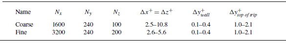


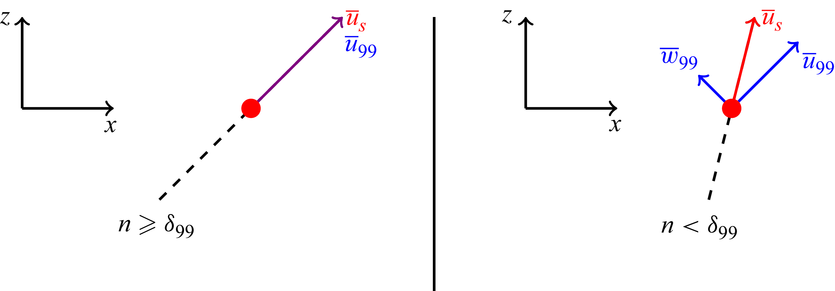


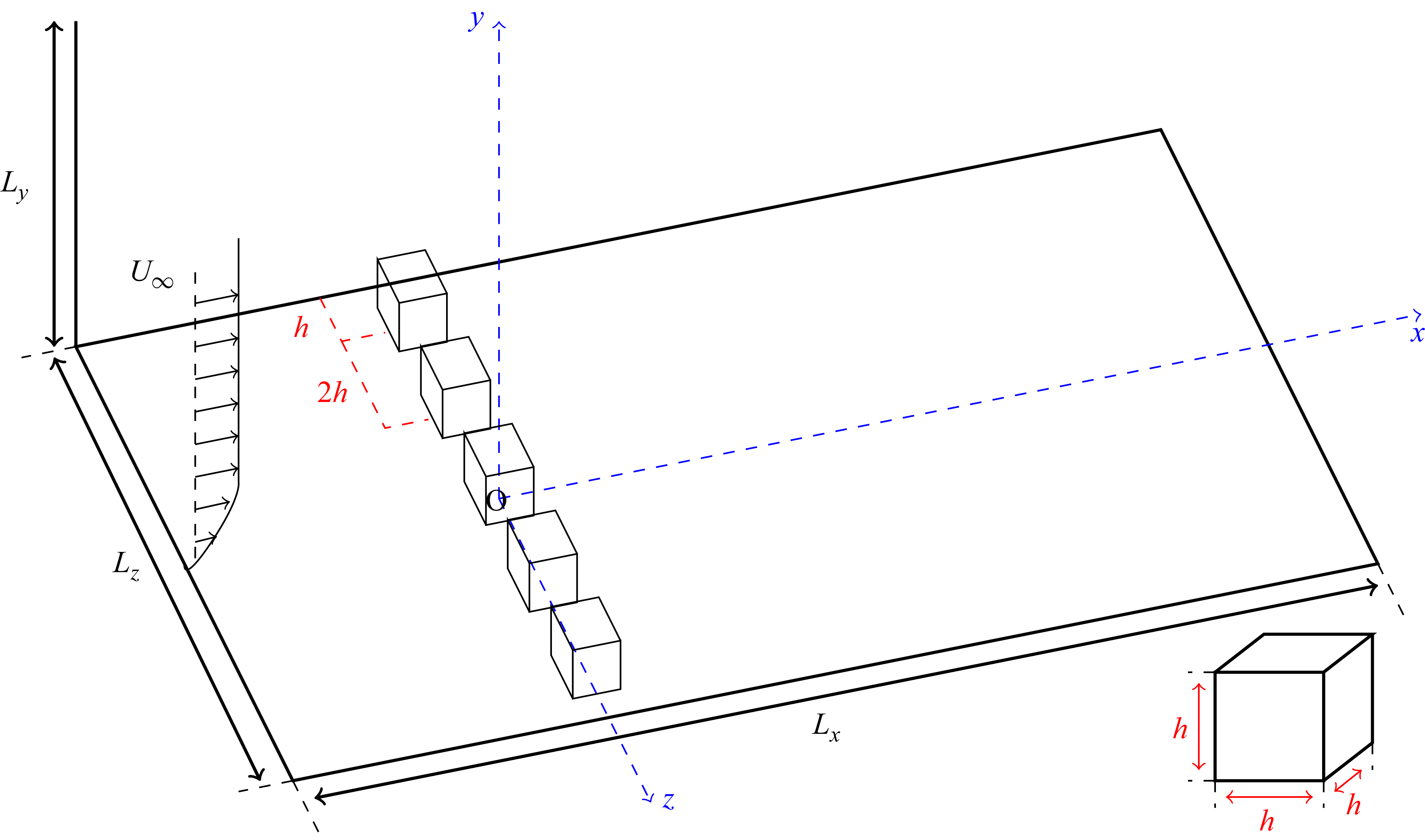
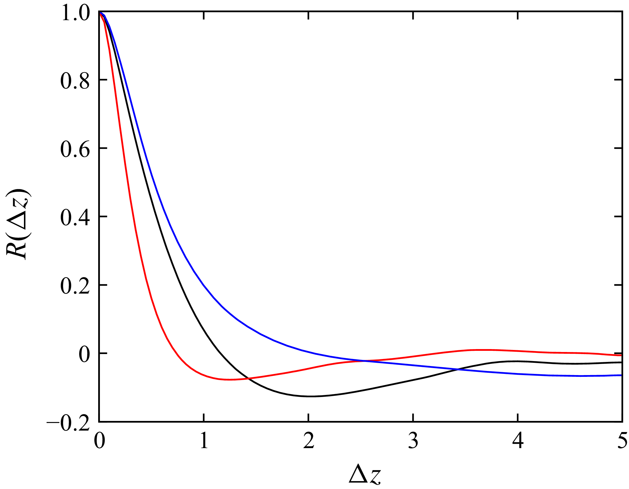


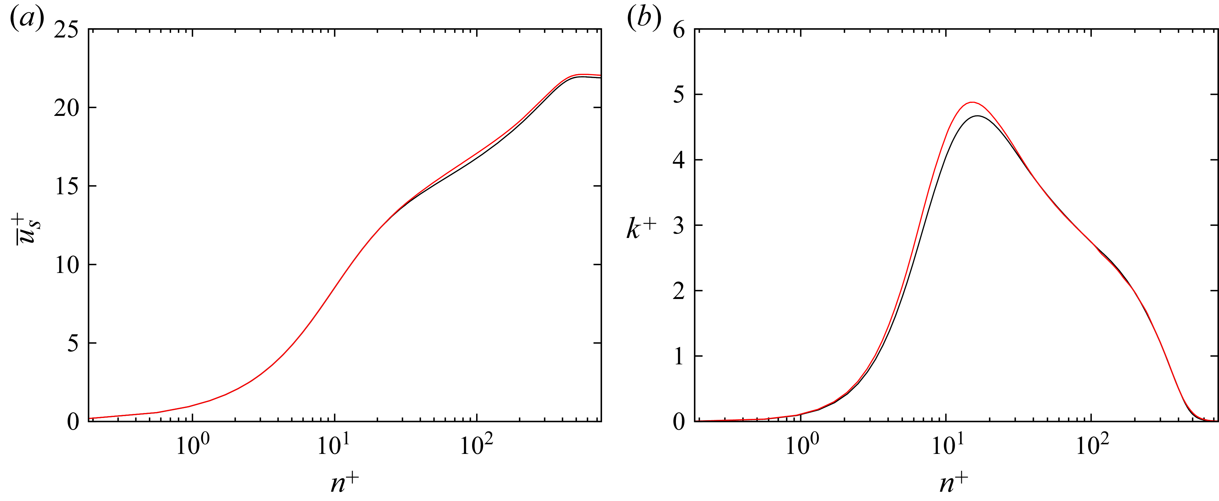


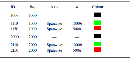
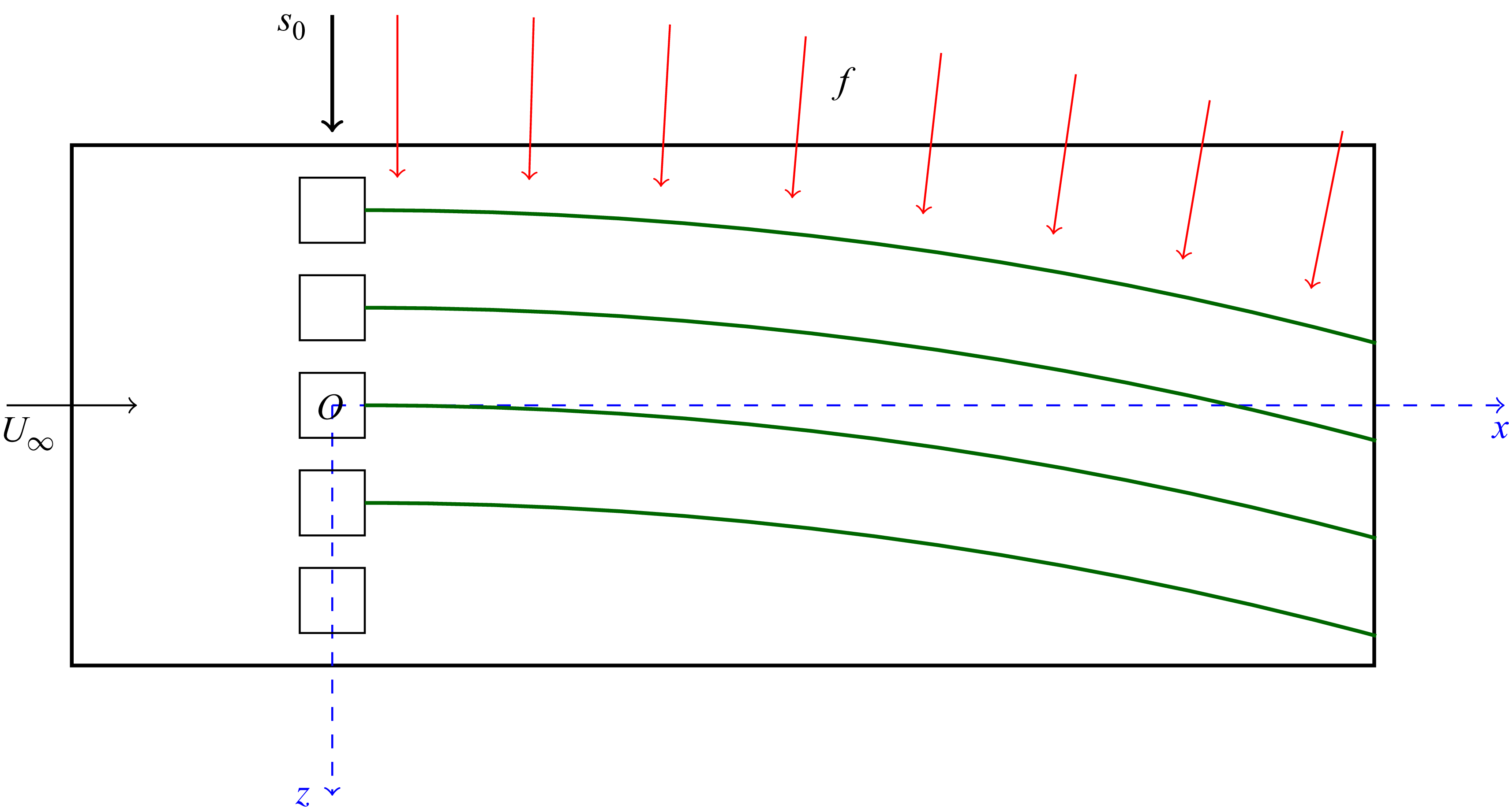


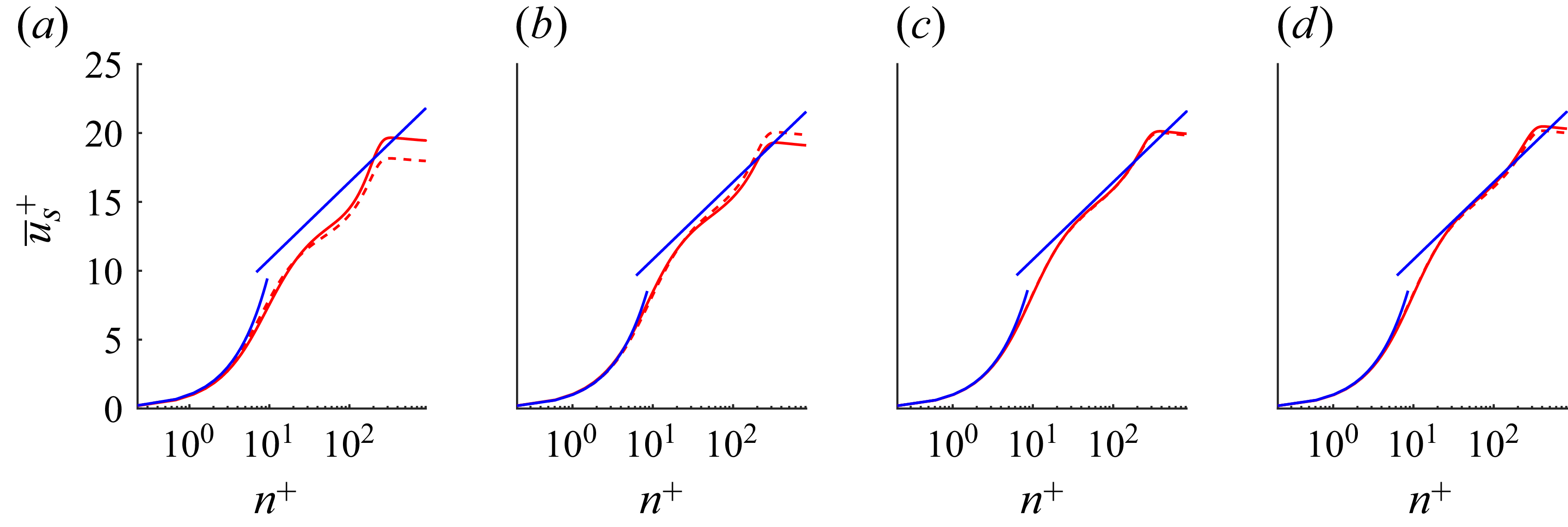


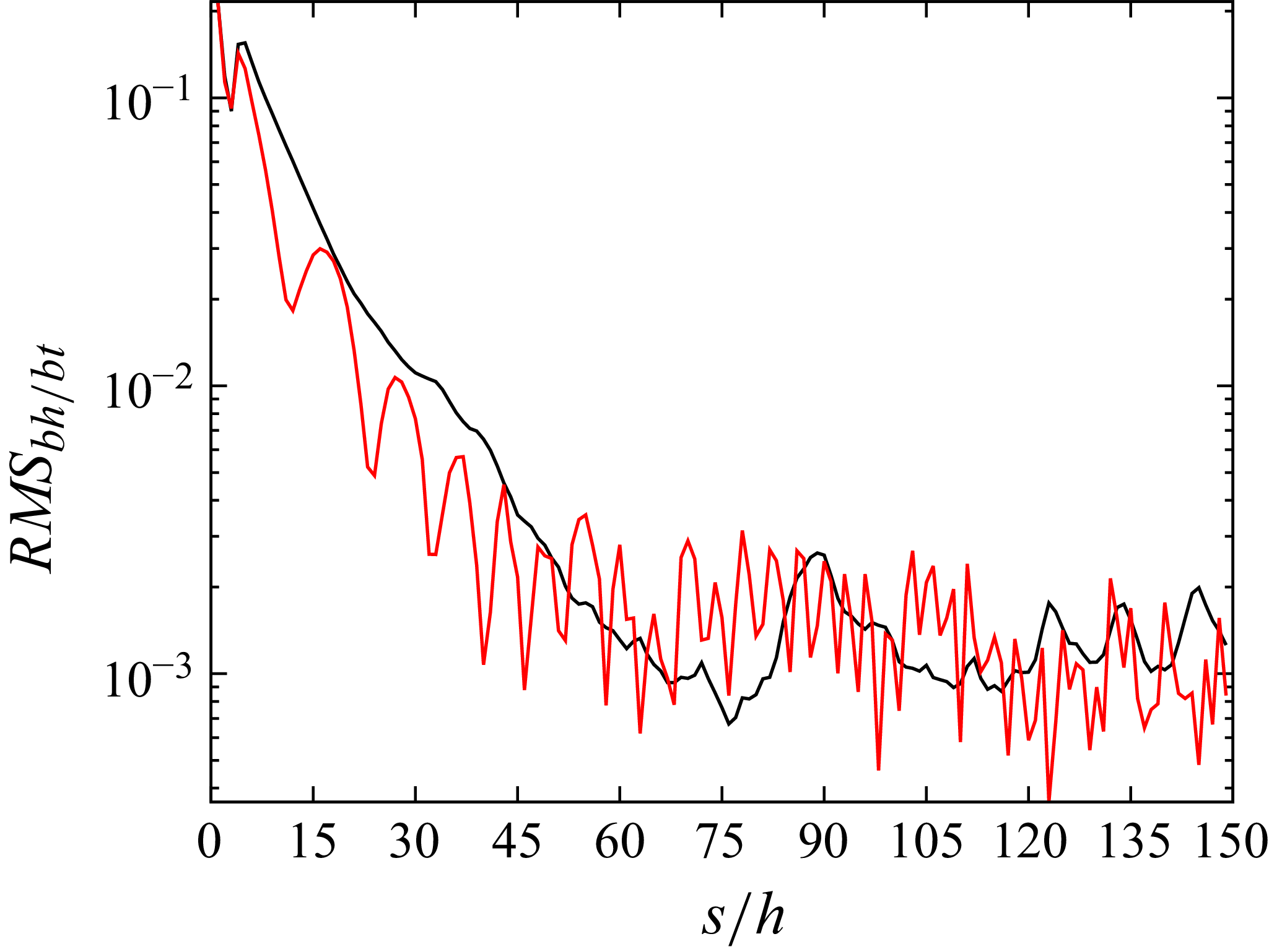


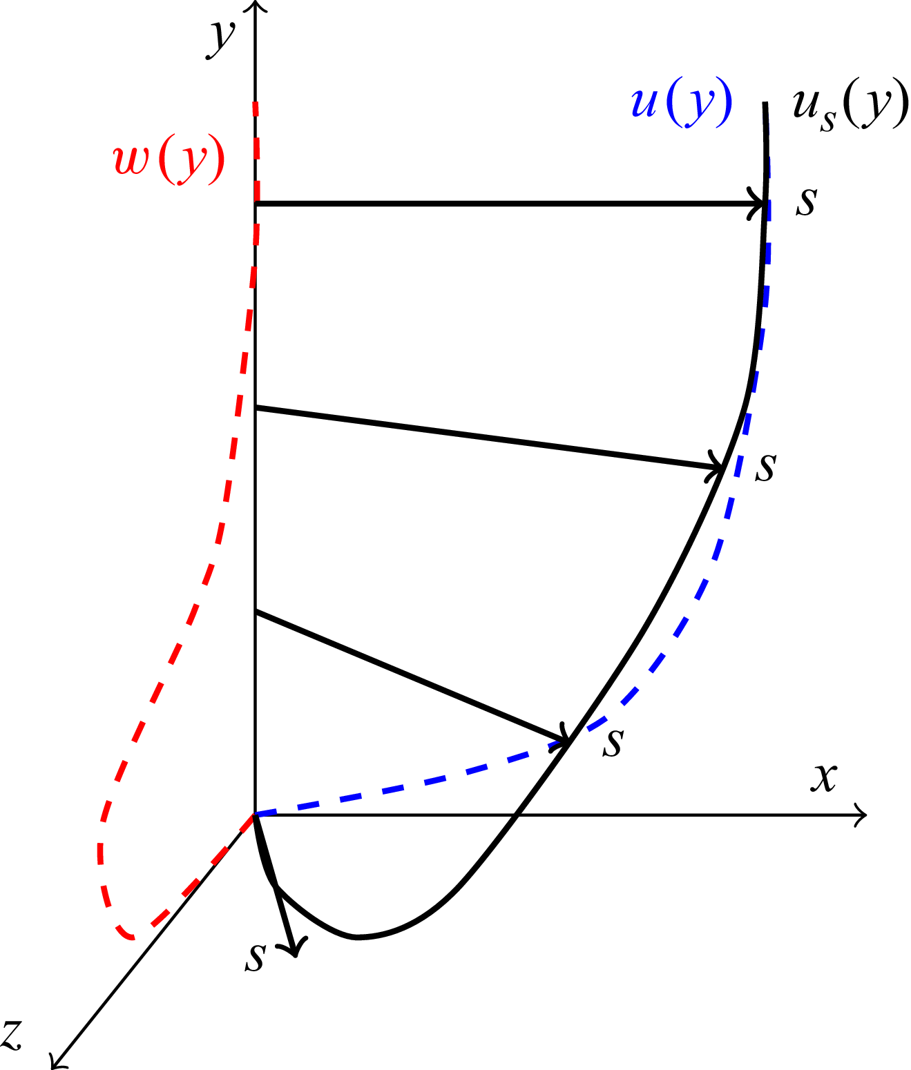
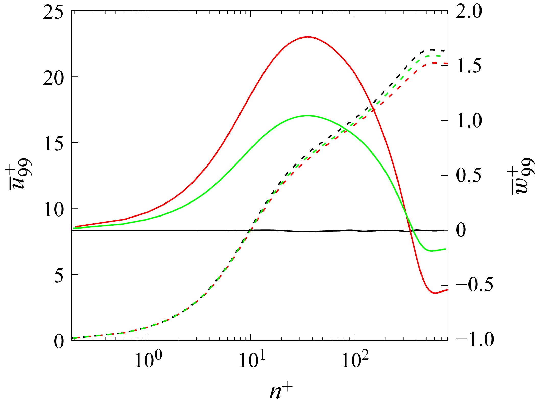

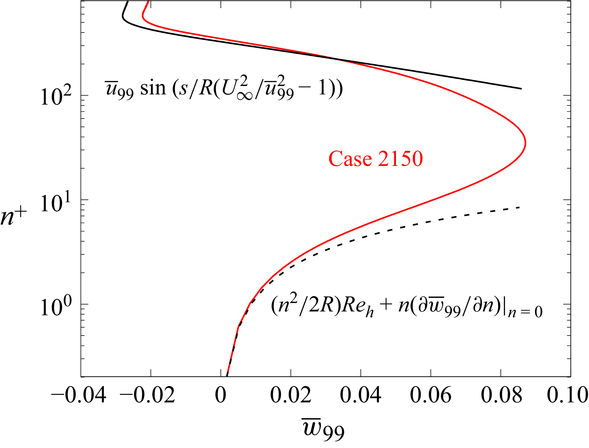

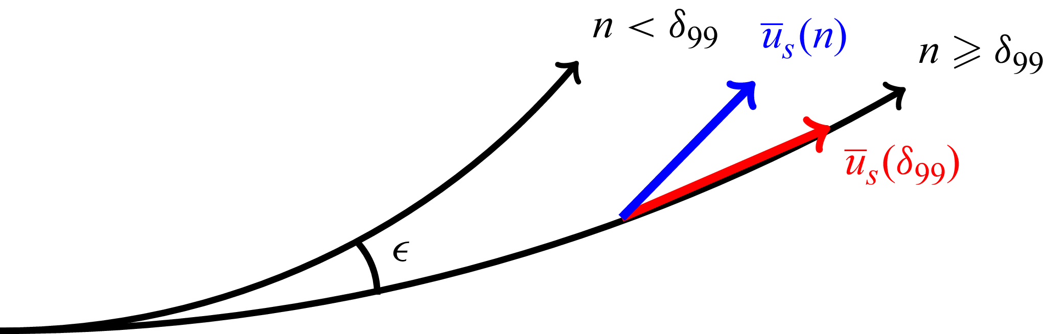
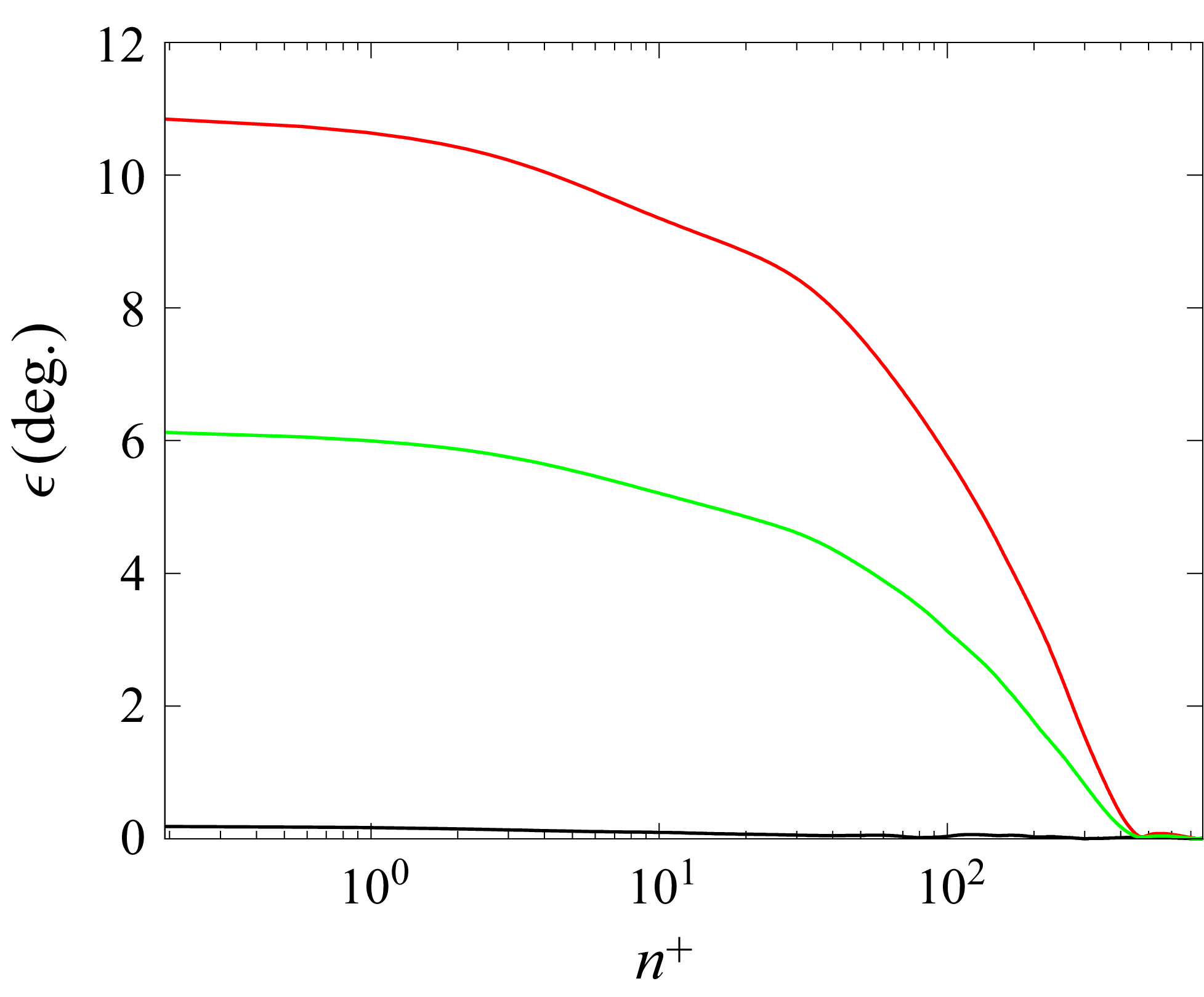

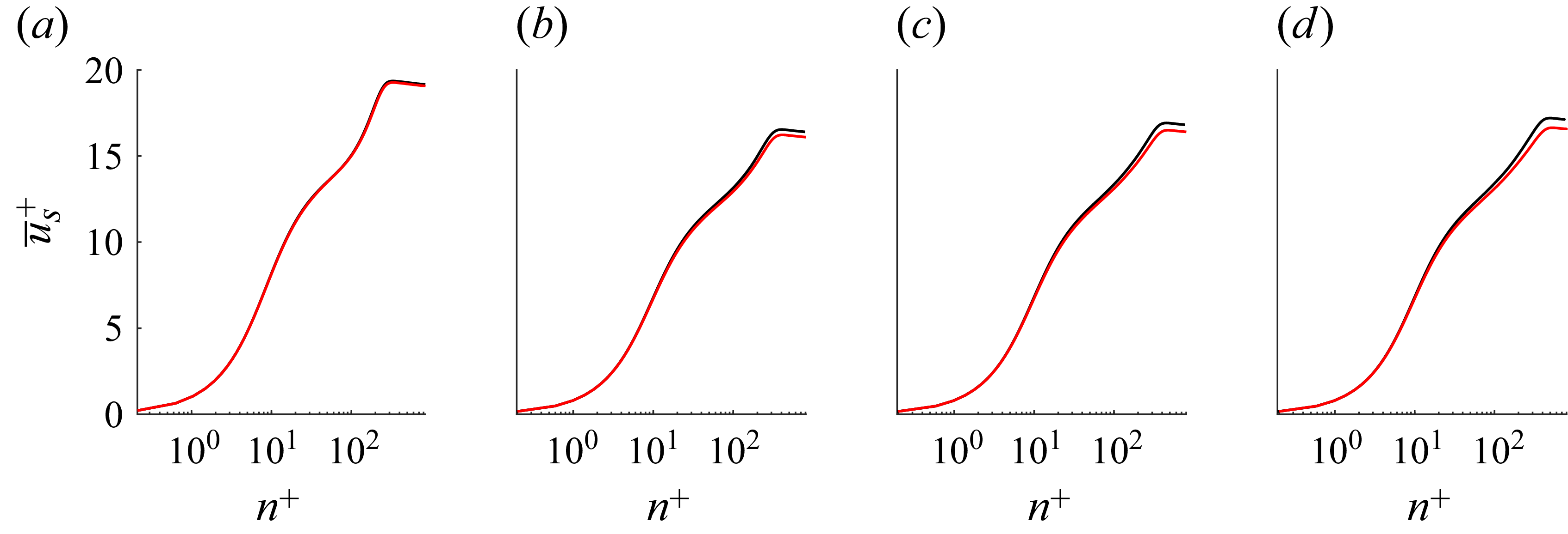


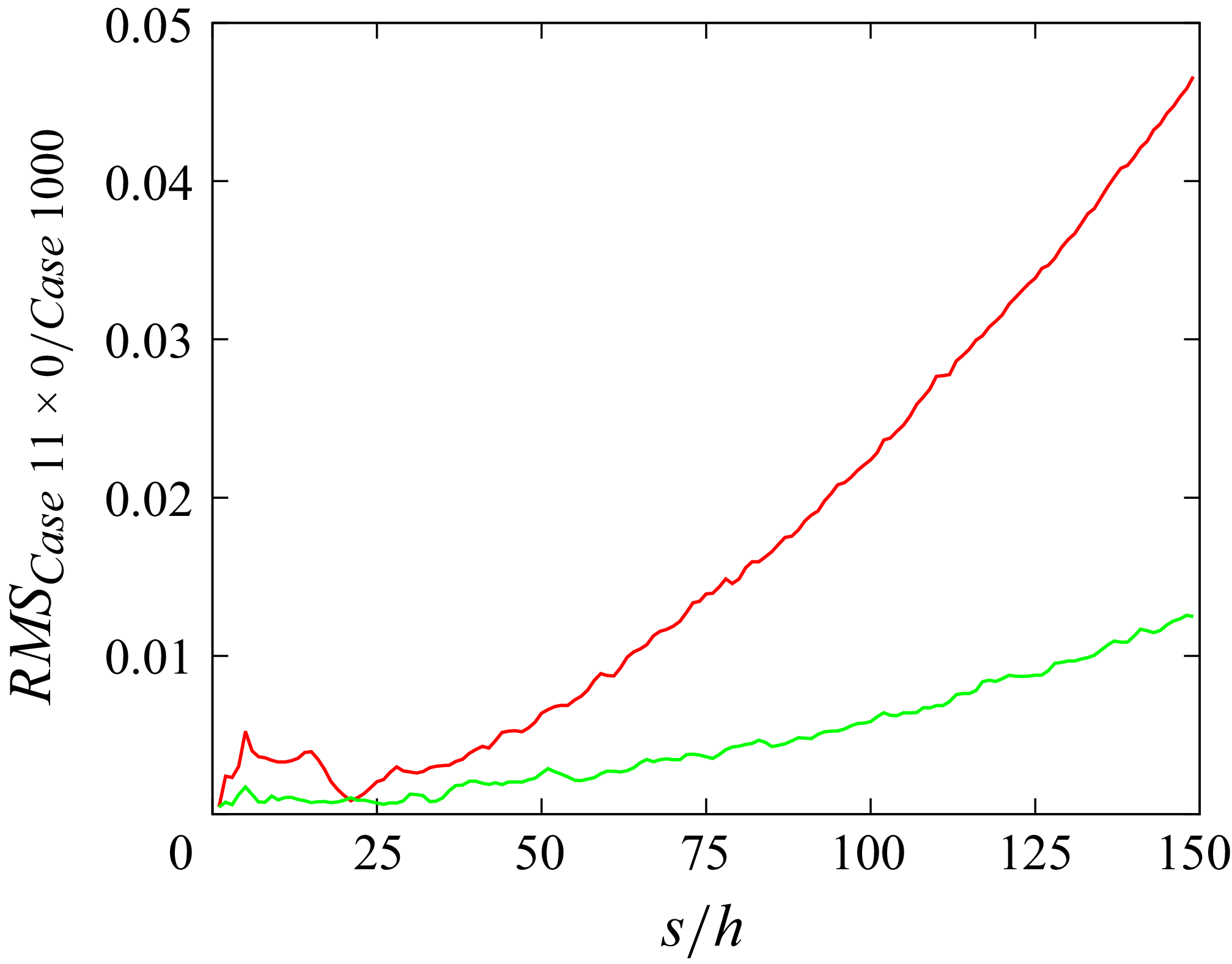
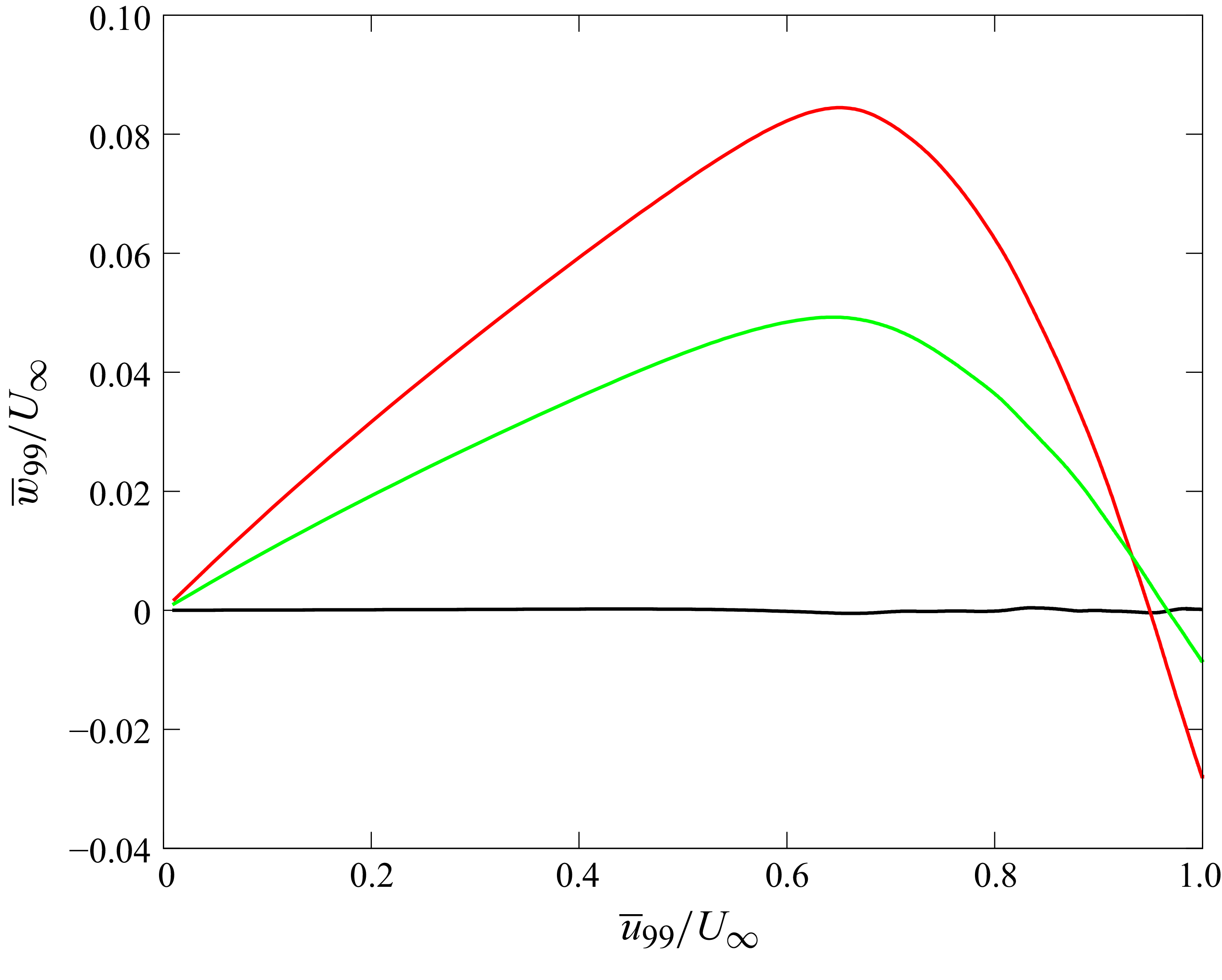


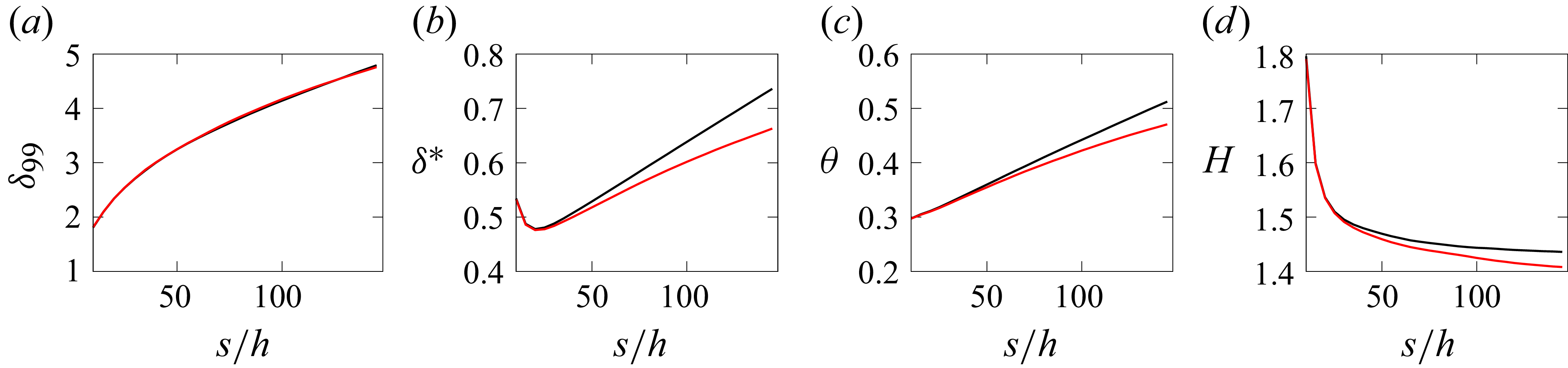


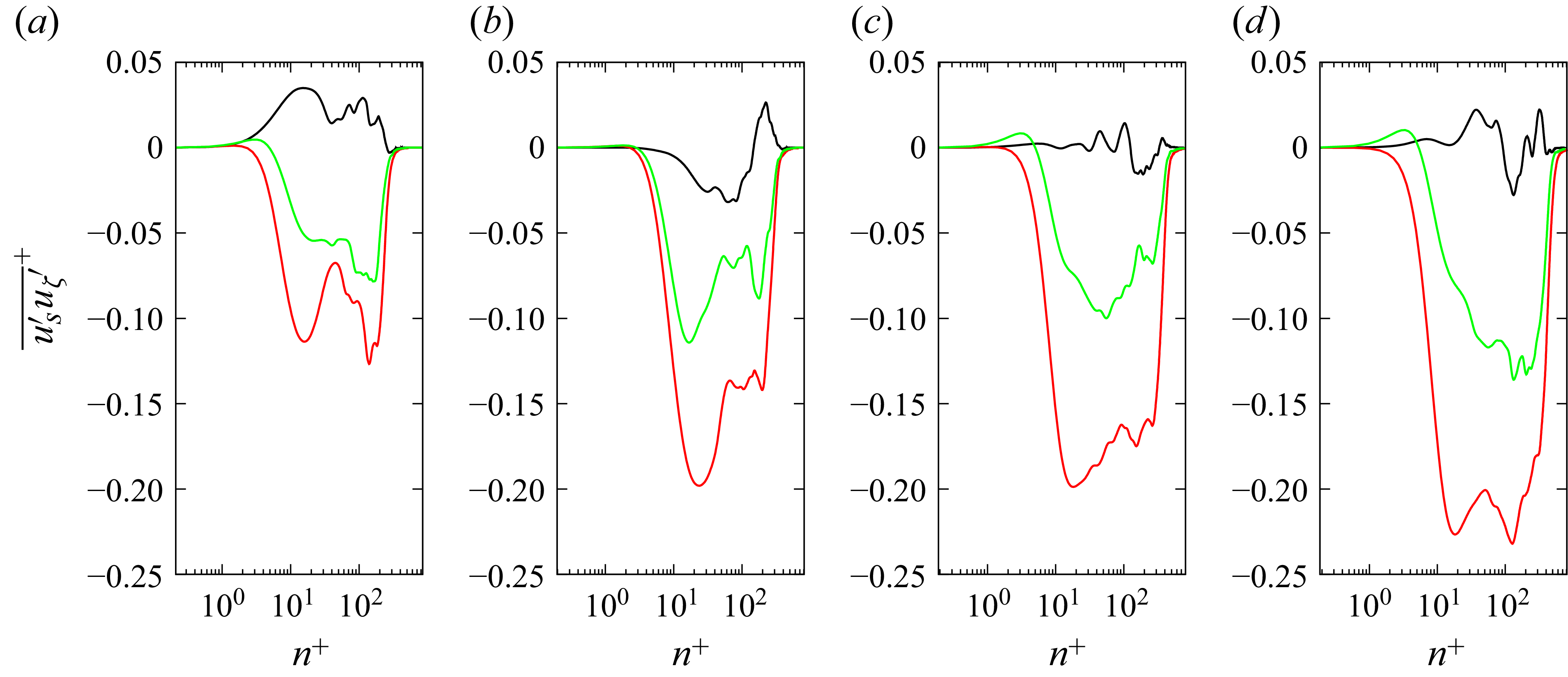


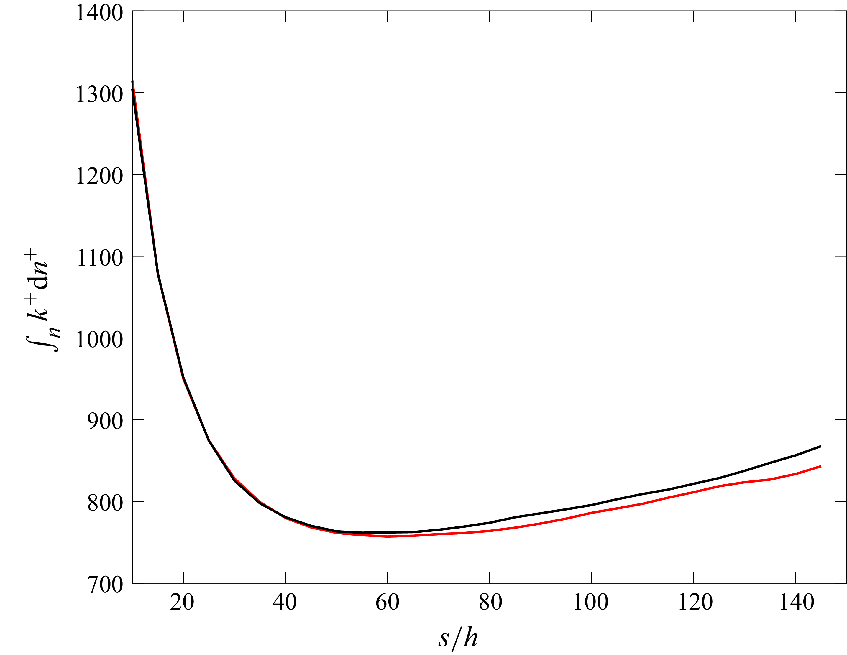


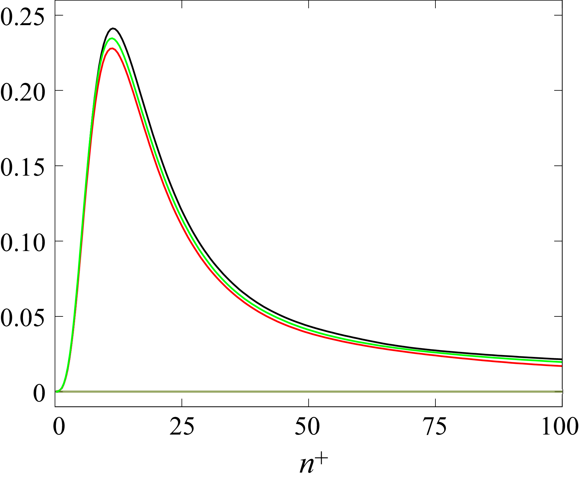


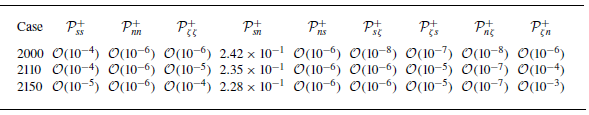


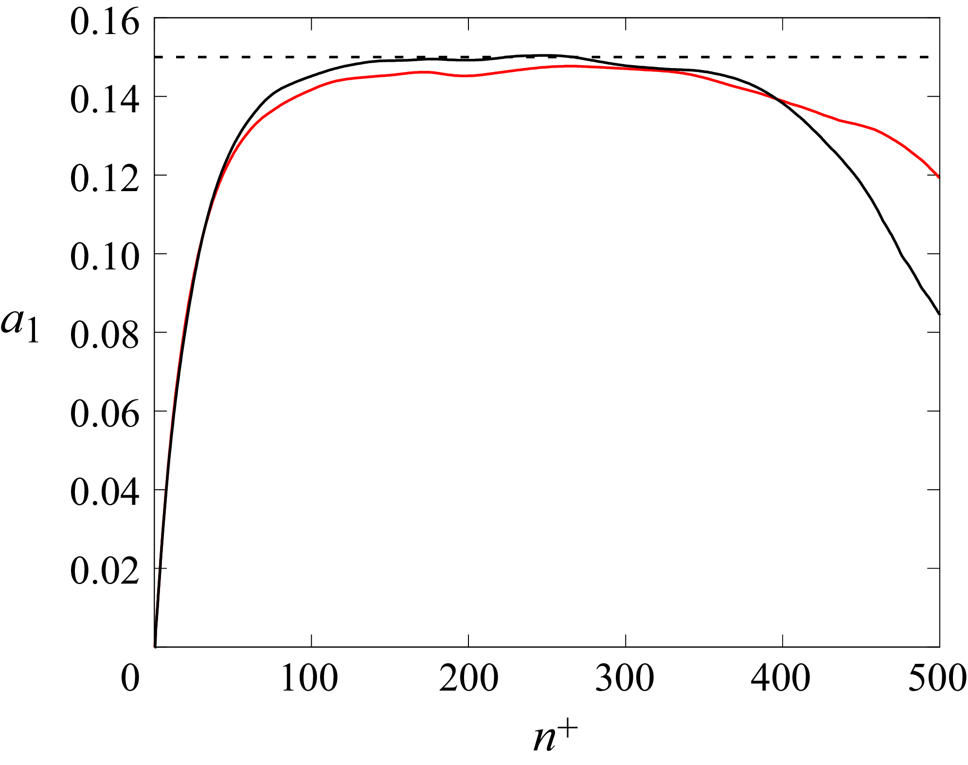


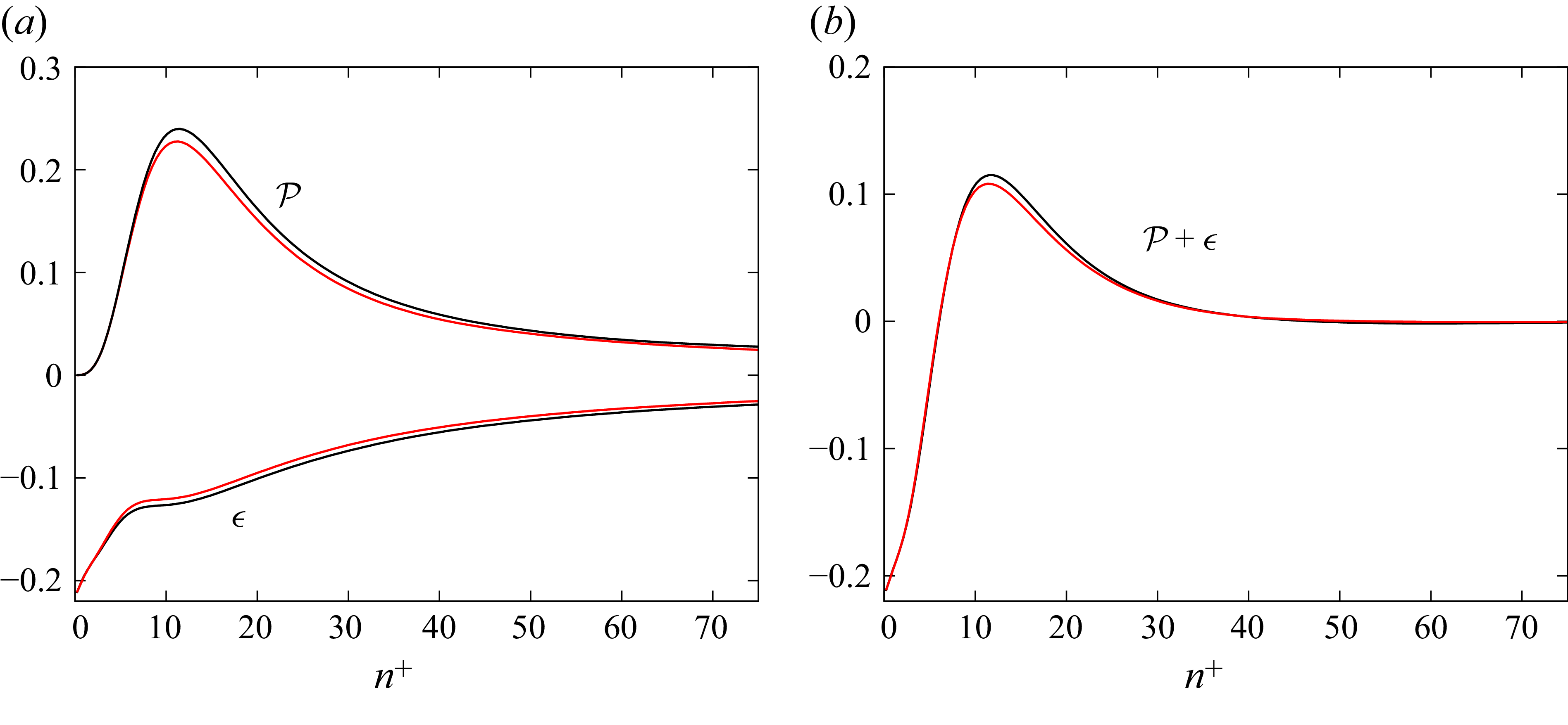

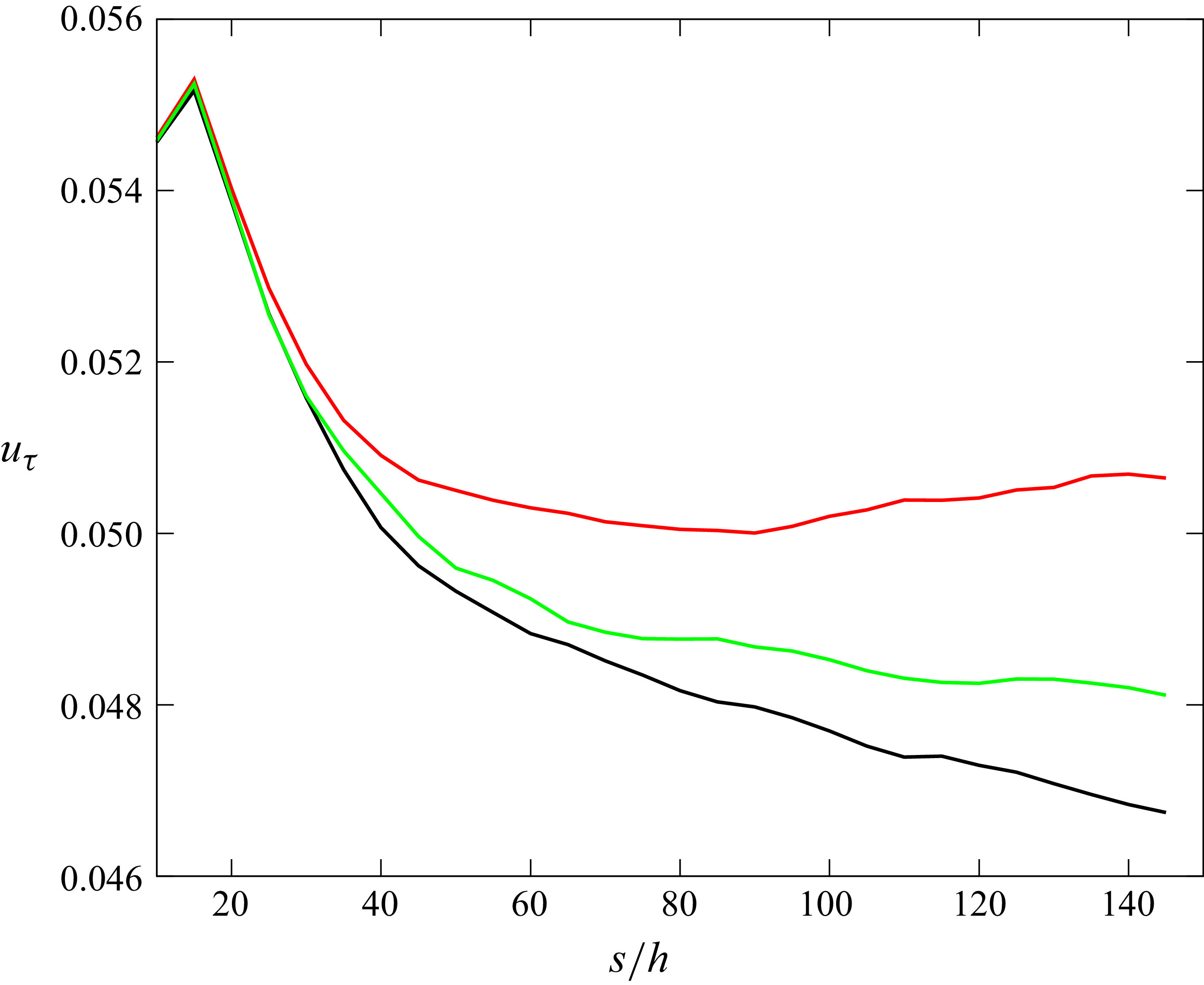
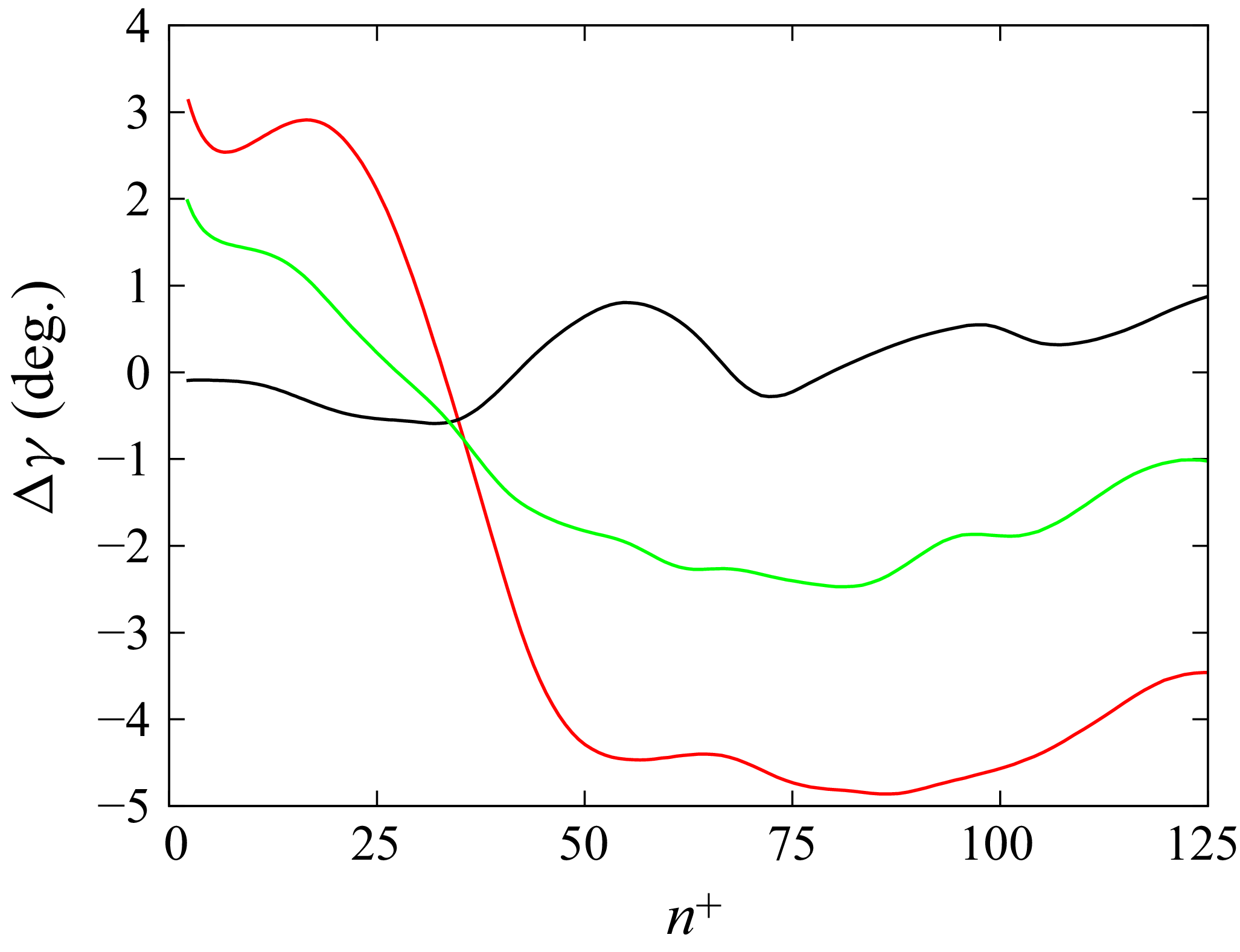


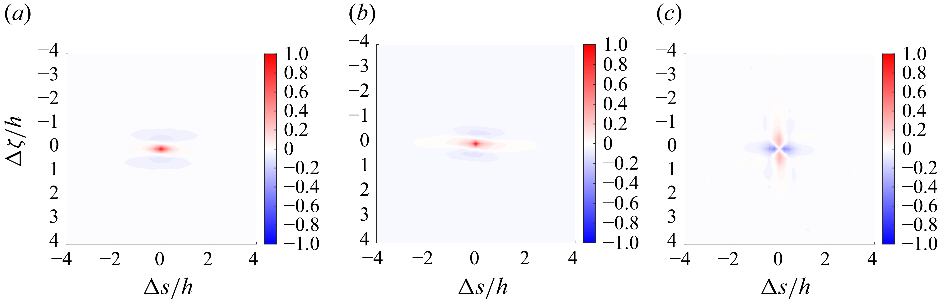


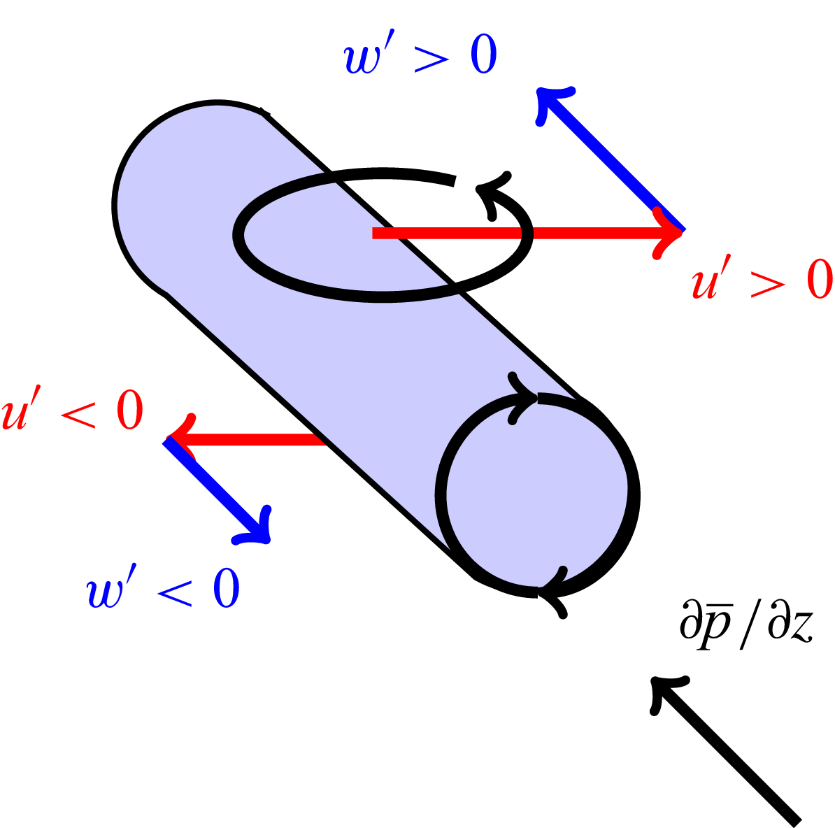
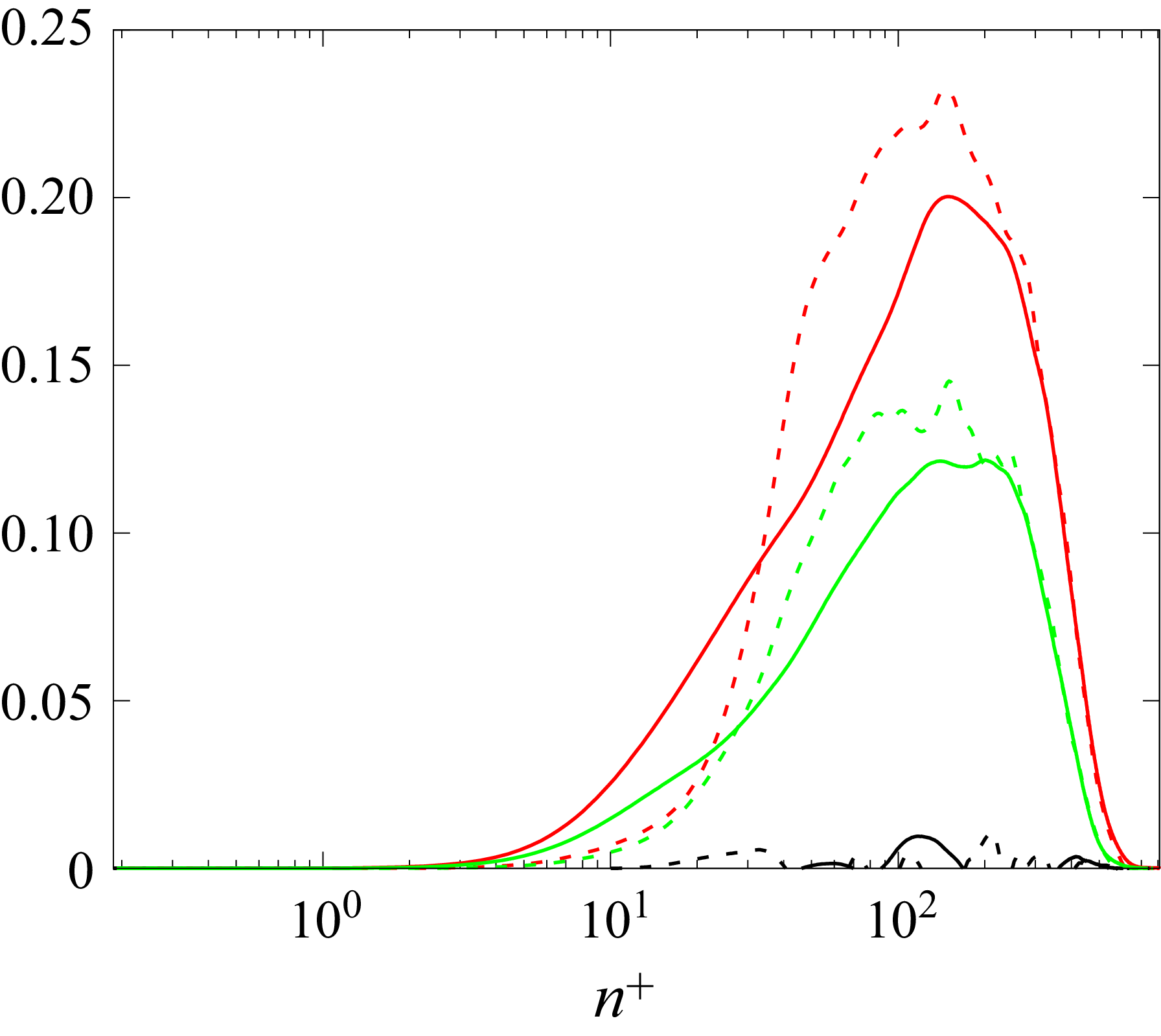


 Open access