


1. Introduction
Glaciers are important indicators for climate change assessment because they are very sensitive to climate variability (Oerlemans, Reference Oerlemans2001). Most of the global glacier volume is contained in the two polar ice sheets and the glaciers and ice caps (GIC) that surround the ice sheets (Frezzotti and Orombelli, Reference Frezzotti and Orombelli2014). Mass loss of GIC in Antarctica and Greenland has contributed to global sea level rise, with more potential in the future (e.g. Meier and others, Reference Meier2007; Hock and others, Reference Hock, de Woul, Radic and Dyurgerov2009; Gardner and others, Reference Gardner2013; Zemp and others, Reference Zemp2019; Hugonnet and others, Reference Hugonnet2021). Glacier inventories provide important baseline data for determining specific changes of glacier area/volume and contribution to sea level in response to climate change (Rastner and others, Reference Rastner2012). Investigation of glacier variability requires a multi-period inventory, and accurate determination of their attributes requires accurate mapping of glacier boundaries and subdivision of glacier complexes into individual glaciers.
The Global Land Ice Measurements from Space initiative (GLIMS; National Snow and Ice Data Center (NSIDC), 2022) aims to collect the derived outlines of the world's glaciers, record and store geospatial information about glaciers, and analyze glacier extent and change (Raup and others, Reference Raup2007). There are two GLIMS vector databases with complete content and comprehensive coverage that provide detailed two-dimensional (2D) outlines and attribute information for GIC in Antarctica and Greenland:
-
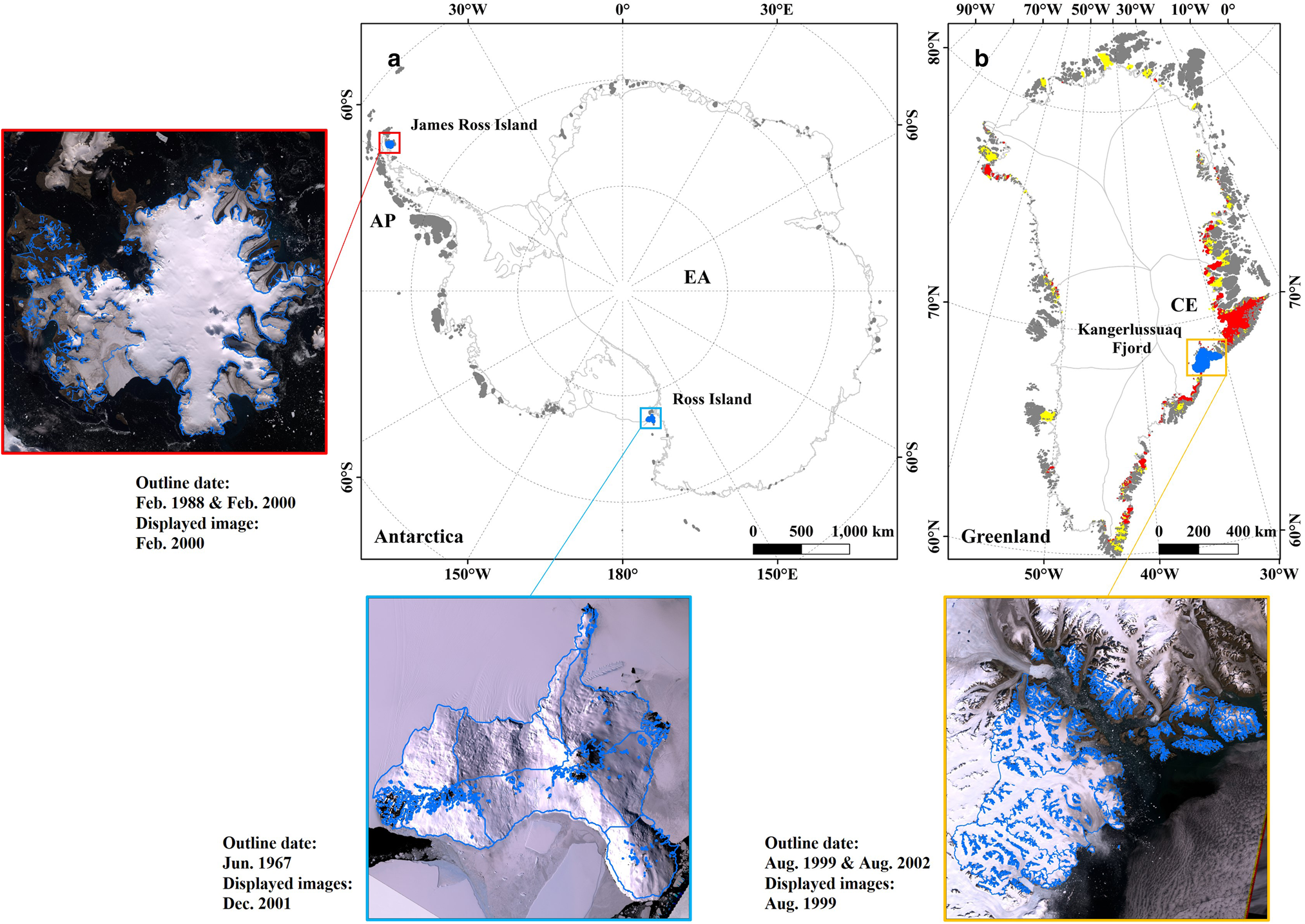
Antarctica: Bliss and others (Reference Bliss, Hock and Cogley2013) compiled an inventory of GIC on the periphery of Antarctica (Fig. 1a), excluding ice rises. Glacier outlines (1957–2005) were derived primarily from manually created polygon files representing coastlines and rock areas from the Antarctic Digital Database (ADD; https://www.add.scar.org/). Watersheds of glaciers were created from previous digital elevation models (DEMs; e.g. Radarsat Antarctic Mapping Project (RAMP) DEM; https://nsidc.org/data/nsidc-0082/versions/2; Liu and others, Reference Liu, Jezek, Li and Zhao2015). Since the island glaciers were considered separate from the continental ice sheet (Hock and others, Reference Hock, Maussion, Marzeion and Nowicki2022), connectivity levels (CLs) of glaciers in this region should theoretically be all CL0 (i.e. no connection).
-
Greenland: Rastner and others (Reference Rastner2012) compiled an inventory of local GIC in Greenland (Fig. 1b). They presented the first comprehensive inventory of Greenland GIC based on semi-automatic glacier mapping techniques and Landsat scenes (most ETM+ scenes from 1999 to 2002), mainly using the Greenland Ice sheet Mapping Project (GIMP) DEM (https://nsidc.org/data/nsidc-0645/versions/1; Howat and others, Reference Howat, Negrete and Smith2015) for watershed analysis and glacier division. Meanwhile, the inventory defines the CL of each glacier with the ice sheet (i.e. CL0; CL1: weak connection (clearly separated by drainage divides in the accumulation region, unconnected or only in contact in the ablation region); CL2: strong connection (difficult to separate in the accumulation region and/or converge in the ablation region)) (Rastner and others, Reference Rastner2012).
Previous inventories and regional coverage map of GIC in Antarctica and Greenland (CL0: dark gray; CL1: yellow; CL2: red). The boxes show the locations of test areas for updating glacier outlines for the new period in this study. The enlarged images show the previous glacier outlines from RGI 6.0 in test areas.
These inventories fill important gaps in the Randolph Glacier Inventory (RGI) 6.0, which is a one-time snapshot of global glaciers that is supplemental to the multi-temporal database of GLIMS (Pfeffer and others, Reference Pfeffer2014), and help to analyze the specific characteristics of these glaciers and model the associated impacts to determine the mass balance of glaciers individually or globally, as well as their impacts on sea level rise (e.g. Huss and Farinotti, Reference Huss and Farinotti2012; Bolch and others, Reference Bolch2013; Gardner and others, Reference Gardner2013; Zemp and others, Reference Zemp2019; Hugonnet and others, Reference Hugonnet2021).
So far, only a few studies have investigated localized GIC changes in Antarctica and Greenland from the standpoint of glacier inventory (e.g. Jiskoot and others, Reference Jiskoot, Juhlin, St Pierre and Citterio2012; Cook and others, Reference Cook, Vaughan, Luckman and Murray2014). For the last two decades, complements to these inventories have been lacking due to the high workload required for creating such datasets. Although the inventory of GIC around the Antarctic Peninsula (AP) has been updated, their source date is still limited to 2000–02 (Huber and others, Reference Huber, Cook, Paul and Zemp2017). There are some updates for parts of the regions on the periphery of Greenland and Antarctica in the just released RGI 7.0 (RGI Consortium, 2023), but most glaciers have not been updated from the well-known RGI 6.0. Updating or creating accurate glacier outlines is extremely difficult in polar areas, as glaciers with all CLs in Greenland and glaciers discharging into ice shelves in Antarctica, as well as ice-debris landforms, are common. Some of these challenges have been discussed (e.g. Paul and Kääb, Reference Paul and Kääb2005; Rastner and others, Reference Rastner2012; Bliss and others, Reference Bliss, Hock and Cogley2013), in general, there is still a lack of detail and clarity on the mapping challenges and their solutions for complex polar regions, especially in Antarctica.
Although previous glacier inventories have been established, existing techniques, such as the use of coherence images and ice velocity maps to support the glacier mapping, had not been effectively applied at the time of their creation. The positioning accuracy and resolution of the source material limit the accuracy of individual glacier outlines, and it is unclear how improved positioning, vertical accuracy and spatial resolution of remote-sensing data used in Antarctica and Greenland could facilitate the definition of improved glacier inventories there. Furthermore, the impact of terminus types and sensor types on polar glacier mapping results is rarely studied, even if it may introduce an uncertainty in updating results and future analysis in glacier change. Another question is whether existing datasets can help in the task of updating glacier inventories.
This study presents a detailed demonstration of selected case studies to better understand the above difficulties and help update glacier inventories in Antarctica and Greenland. We synthesize existing techniques and new source data to update the inventories of selected GIC for new time periods, which are located at the periphery of the two ice sheets. We update a glacier inventory using a well-established workflow that includes mapping glacier boundaries, subdividing glaciers by watersheds and assigning attributes. The mapping solutions for complex glacier scenarios are discussed and the precision or uncertainty of glacier outlines is evaluated, taking James Ross Island beside the AP, Ross Island in East Antarctica (EA) and the glacier scene around Kangerlussuaq Fjord in central east (CE) Greenland as test regions (Fig. 1). We compare the results and methods to the previous inventory in these regions. We also highlight the challenges in upscaling these techniques in order to complete full inventories in the study area.
2. Source data
In view of updating the GIC inventories in the study areas, it is necessary to consider the reliable remote-sensing data that are available for the analysis period (i.e. last two decades). The source data information used in the applications and discussions of this study is listed in Tables S1–S3.
2.1 Optical images
Medium- to high-resolution optical satellite sensors such as Landsat 4/5 TM, Landsat 7 ETM+, Landsat 8 OLI and ASTER are commonly used for mapping glaciers (Winsvold and others, Reference Winsvold, Kaab and Nuth2016). However, the small image extent of ASTER (60 × 60 km) limits its ability to map glaciers over a large region in the study area, especially in Greenland, where the optimal threshold for ratio images in the semi-automatic mapping method must be selected for each scene. The Landsat image archive represents the longest continuous satellite record and has sufficient resolution to track glacier changes, making it useful for glacier mapping (Winsvold and others, Reference Winsvold, Kaab and Nuth2016). Landsat Level 1 T (L1 T) satellite imagery with resolutions up to 30 m (multispectral) or 15 m (panchromatic) was used to update glacier inventories in test areas. This dataset is available on the United States Geological Survey (USGS) Earth Explorer website, and its T1-level data provide consistent geographic calibration within prescribed tolerances (<12 m root mean square error (RMSE); https://earthexplorer.usgs.gov/). The presence of striping problems in ETM+ scenes after 2003 due to the scan line corrector affects the mapping of glaciers, so we primarily used Landsat 8 OLI to map glaciers since 2013. We selected less cloudy images taken during summer time in Antarctica and Greenland to obtain sufficient light for the scenes and to reduce the impact of seasonal snow on glacier mapping. To further exclude clouds, snow and shadows and to fully represent and accurately map the glaciers, we referenced multiple images alternately. OLI bands 6, 5 and 4 were each used in RGB (red, green, blue) channels, respectively, to generate contrast-enhanced false-color composites to help correctly identify glaciers (Paul and others, Reference Paul2015).
The correction for seasonal snow is a challenge for creating glacier inventories, regardless of the manual or automatic method used. It is not recommended to use scenes covered by seasonal snow for mapping (Paul and others, Reference Paul2015), and satellite scenes at the end of the ablation season should be selected if possible (Paul and others, Reference Paul2009; Racoviteanu and others, Reference Racoviteanu, Paul, Raup, Khalsa and Armstrong2009). In addition, snow may still fall during summer in the study area. Given these limitations, image selection is always a challenge. Fortunately, in the case of infrequent updates, Landsat OLI offers the opportunity to select better data scenes from the last decade.
The optical data in Google Earth, which come from optical sensors such as QuickBird and Worldview, can be very high-resolution (better than 1 m) (Molg and others, Reference Molg, Bolch, Rastner, Strozzi and Paul2018) and allows for viewing from a three-dimensional (3D) perspective. Therefore, they were used in this study as quality control and accuracy verification for glacier mapping if available. The Landsat Image Mosaic of Antarctica (LIMA; https://lima.usgs.gov/; Bindschadler and others, Reference Bindschadler2008) and the New Image Mosaic of Greenland (http://data.tpdc.ac.cn/; Chen and others, Reference Chen2020) serve as a background for orientation in this study. These mosaics are mainly composed of Landsat 7 ETM+ and Landsat 8 OLI imagery and allow us to quickly locate glaciers in the study area.
2.2 Coherence images
Interferometric synthetic aperture radar (InSAR) coherence can be used to accurately map debris-covered glacier margins and is almost independent of weather and solar illumination (Atwood and others, Reference Atwood, Meyer and Arendt2010; Ke and others, Reference Ke2016). InSAR coherence represents the complex correlation between two SAR images and indicates the temporal stability of the backscattered signal, and thus can be used to separate stable and unstable surface regions (Lippl and others, Reference Lippl, Vijay and Braun2018). When most of the seasonal snow has disappeared during summer, glacier flow and melting are responsible for most of the surface-geometry changes, resulting in very low coherence (Frey and others, Reference Frey, Paul and Strozzi2012).
Designed for SAR interferometry applications and displacement monitoring, the Copernicus Sentinel-1 constellation provides free access to SAR images of the same orbit every 12 days over the study area (Strozzi and others, Reference Strozzi2020). In this study, radar data were chosen from the C-band Sentinel-1A and -1B sensors with interferometric wide swath mode (IW) to estimate glacier coherence for the new period. We selected the original SAR single-look complex (SLC) pairs and acquired terrain-corrected and geocoded coherence images processed by the Alaska Satellite Facility (ASF; https://search.asf.alaska.edu/) using GAMMA software and the best publicly available global DEM (Copernicus DEM; 30 m). The 10 × 2 number of looks was selected to obtain products with a pixel spacing of 40 m.
In the case studies, interferograms during summer time were selected to maximize decoherence on glaciers, where surface melting rapidly reduces coherence on the glacier (Atwood and others, Reference Atwood, Meyer and Arendt2010). However, additional glacial indicators in coherence and surface slope are needed to extract decoherence areas and filter out low coherence caused by steep terrain, respectively (e.g. Atwood and others, Reference Atwood, Meyer and Arendt2010; Ke and others, Reference Ke2016; Lippl and others, Reference Lippl, Vijay and Braun2018). We tuned and determined these thresholds to minimize the holes within glaciers and to achieve the fit with most of the confirmed ice pixels in optical scenes. Although water bodies also lead to very low coherence, they can be clearly distinguished in the optical images (e.g. Frey and others, Reference Frey, Paul and Strozzi2012).
2.3 DEMs and ice velocity maps
DEMs can be used for semi-automatic definition of glacier divisions based on flow direction grids and watershed analysis, and for determining glacier attributes (Paul and others, Reference Paul2009; Racoviteanu and others, Reference Racoviteanu, Paul, Raup, Khalsa and Armstrong2009). The Reference Elevation Model of Antarctica (REMA; Howat and others, Reference Howat, Porter, Smith, Noh and Morin2019) and ArcticDEM (Porter and others, Reference Porter2018) were derived from hundreds of thousands of individual stereo DEMs registered vertically to Cryosat-2 and ICESat altimetry, with absolute uncertainties of less than 1 m and relative uncertainties of decimeters over most of the area (https://www.pgc.umn.edu/data/). In the case studies, we used mosaics of these two high-precision DEMs as inputs to generate contours, slope, aspect and flow-direction maps to support the accurate definition of glacier boundaries and watersheds. These mosaics have a 32 m resolution which have essentially the same spatial resolution and are within the same decade as the optical images (Paul and others, Reference Paul2009). In previous inventories, the RAMP DEM has a reported vertical accuracy of about 100–130 m and a horizontal resolution of 200 m in rugged mountainous areas (Liu and others, Reference Liu, Jezek and Li1999), and the GIMP DEM with 90 or 30 m resolution and reported vertical accuracy of about 10 m was used (Rastner and others, Reference Rastner2012; Howat and others, Reference Howat, Negrete and Smith2014). In particular, REMA provides unprecedented resolution and accuracy for Antarctica and the potential to improve the accuracy of glacier inventories.
The delineation of glacier drainage basins at gentle slopes in the study area is challenging because of the accompanied local topographic disturbances and complex ice movement patterns (e.g. Krieger and others, Reference Krieger, Floricioiu and Neckel2020b). Therefore, to supplement DEM data, we additionally used ice velocity maps from SAR data for Antarctica (https://nsidc.org/data/nsidc-0484/versions/2; Rignot and others, Reference Rignot, Mouginot and Scheuchl2017) and Greenland (https://nsidc.org/data/nsidc-0478/versions/2; Joughin and others, Reference Joughin, Smith, Howat and Scambos2015) to guide glacier division. The direction of ice flow may indicate a different direction than the aspect due to glacier instability, bedrock features and ice volume interactions (Krieger and others, Reference Krieger, Johnson and Floricioiu2020a). In addition, the magnitude of the ice velocity indicates intuitively its acceleration from the accumulation zone to the ablation zone, thus assisting in delineating the individual glacier extent.
3. Methods
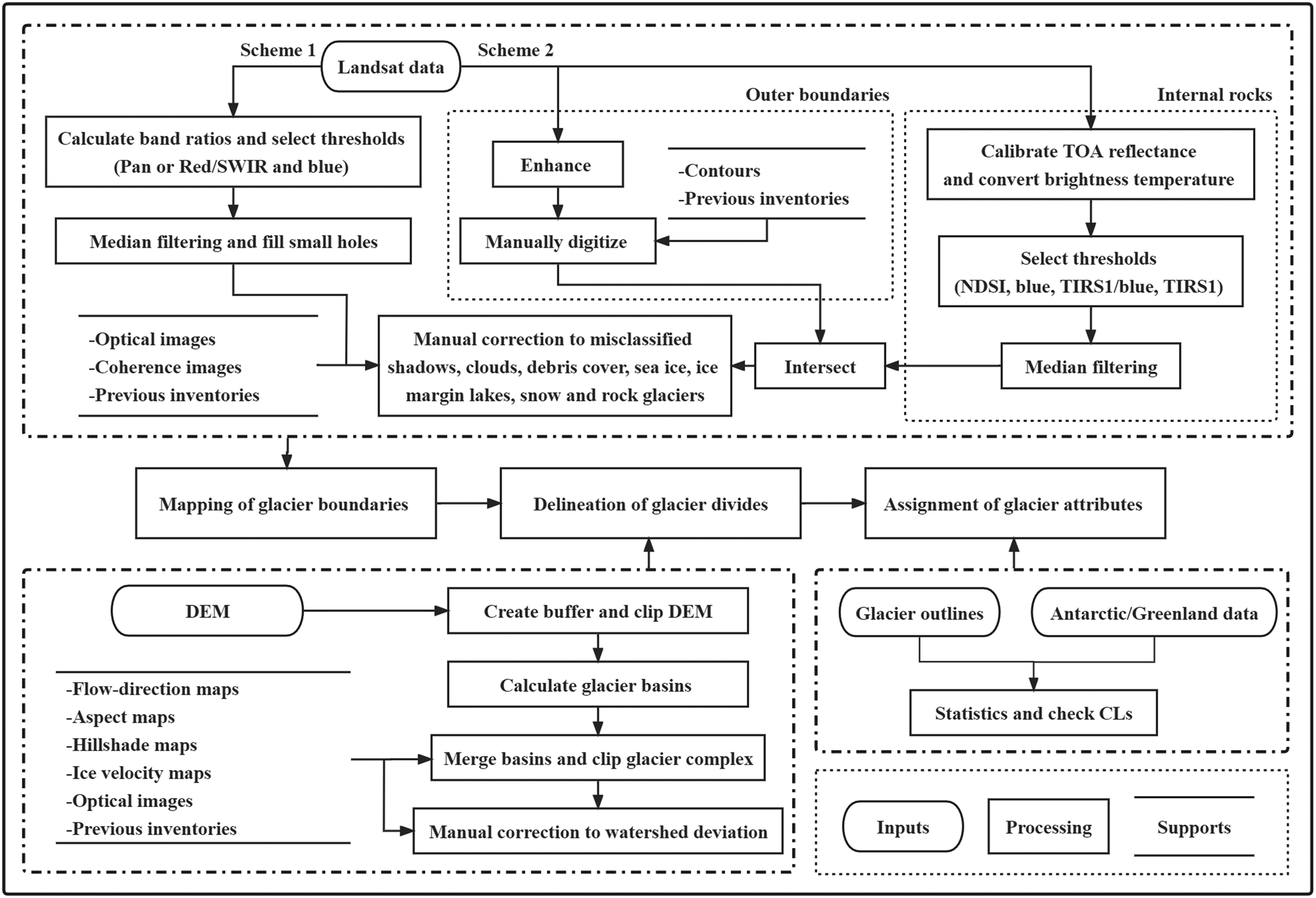
Glacier outline generation involves three main steps: (1) mapping glacier boundaries, (2) delineating glacier divides and (3) assigning glacier attributes (Fig. 2). All calculations are performed using ArcGIS version 10.5 and ENVI version 5.3 with various toolboxes available. The type of map projection of the layers is ‘WGS84 Antarctic Polar Stereographic’ in Antarctica and ‘WGS84 NSIDC Sea Ice Polar Stereographic North’ in Greenland. Figure 2 illustrates our technical workflow, and the three main steps are described in more detail in the following sections.
Framework for updating glacier inventories in this study, including three modules (mapping of glacier boundaries, delineation of glacier divides and assignment of glacier attributes).
3.1 Mapping of glacier boundaries
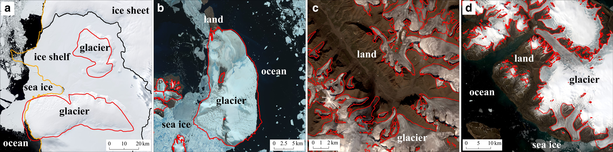
In Antarctica, individual glaciers can be very large (up to 6000 km2) and their terminus characteristics are unique (Bliss and others, Reference Bliss, Hock and Cogley2013). A large fraction of glaciers share a common boundary with ice shelves (Fig. 3a). However, the same spectral properties prevent automatic classification methods from separating them, implying that manual interpretation is necessary to map most or even the whole glacier boundary. The ocean terminus indicates that the glacier boundary line is coincident with the coastline and the land-terminating boundaries normally represent the peripheral retreat of island glaciers and the exposure of internal rocks (Fig. 3b). Automatic classification methods are well applicable to extract land-terminating or marine-terminating glacier boundaries with less sea ice and seasonal snow influence in Antarctica. This is the case for Greenland, where most glaciers terminate on land (Fig. 3c), and some ice caps (e.g. Flade Isblink ice cap) and narrow outlet glaciers are marine-terminating (Fig. 3d). Glaciers are generally clearly separated from the land and ocean during the melting period, so that initial glacier boundaries can be automatically derived to facilitate manual correction (e.g. Rastner and others, Reference Rastner2012).
Examples of terminus characteristics of glaciers in the study areas. The red glacier boundaries are from RGI 6.0, with Landsat OLI scenes in (a) West Antarctica (WA) (72.8$^\circ$ S, 90.4$^\circ$
 W), (b) AP (64.5$^\circ$
 S, 57.2$^\circ$
 W), (c) central west (CW) of Greenland (69.9$^\circ$
 N, 53.6$^\circ$
 W) and (d) northwest (NW) of Greenland (76.8$^\circ$
 N, 69.3$^\circ$
 W). The orange and black lines in (a) represent the coastlines and grounding lines, respectively.
Greenland has extensive debris cover over glacierized areas (Herreid and Pellicciotti, Reference Herreid and Pellicciotti2020), which poses a significant mapping challenge. In contrast, most Antarctic glaciers are ice caps, which means that there is generally no debris that can fall from the rock walls onto the glacier (the glacier scenario on James Ross Island in Case Study 2 is an exception). The current climatic circumstances, which include sustained subfreezing conditions and a lack of diurnal circulation, reduce the amounts of debris produced by freeze–thaw activity. Therefore, the largely debris-free conditions make the classification of nunataks contained within the glacier possible (e.g. Burton-Johnson and others, Reference Burton-Johnson, Black, Fretwell and Kaluza-Gilbert2016).
To overcome the ground conditions and mapping challenges in glacial regions, manual interpretation and well-established automatic methods were combined to extract glacier boundaries. Two schemes were considered to map glaciers that share different length proportion boundaries with ice shelves or sea ice. The difference between the two schemes is whether the visual interpretation method is best used for post-processing the automatically derived boundaries or for mapping the initial glacier outer boundaries. It should be noted that glacier boundaries can be visually interpreted in any case and the two schemes can be complementary to each other to cope with different glacier situations over a wide study area when taking into account the efficiency of polygon editing.
Scheme 1: The well-established semi-automatic band ratio method was adopted to map glaciers with a large proportion of land terminus and less sea ice attached ocean terminus (Case Studies 1 and 3). Glacier classification using threshold segmentation of the Landsat TM band raw data ratio (e.g. TM3/TM5) has proved to be the most effective method for mapping glaciers (Paul and others, Reference Paul, Kääb, Maisch, Kellenberger and Haeberli2002). The optimal ratio threshold should be found for each glacier scene (Rastner and others, Reference Rastner2012) and an additional threshold in the blue band can be introduced to improve the mapping of shaded glaciers, which have higher reflectance than bare rock (Paul and Kääb, Reference Paul and Kääb2005; Paul and Andreassen, Reference Paul and Andreassen2009). We applied the scheme proposed by Paul and others (Reference Paul, Winsvold, Kaab, Nagler and Schwaizer2016) to replace the 30 m spatial resolution red band (OLI4) with a 15 m resolution panchromatic band (OLI8) for glacier mapping (OLI8/OLI6) to automatically draw glacier boundaries at higher spatial resolution. To calculate the ratio, the spatial resolution of the OLI6 image was improved to 15 m by bilinear interpolation. A median filter (3 × 3 kernel) was applied to smooth the glacier boundary and this process is considered to have little influence on the final glacier areas (He and Zhou, Reference He and Zhou2022). However, higher resolution data are usually accompanied by higher processing workload (Paul and others, Reference Paul, Winsvold, Kaab, Nagler and Schwaizer2016), as more dirty ice, fine rock outcrops and debris-covered areas are identified in detail, causing many small holes in the glacier polygons. Therefore, the polygon part elimination tool in ArcGIS was additionally used to eliminate these extremely small holes (area <0.003 km2) in the glacier polygons at an OLI resolution of 15 m to reduce the processing effort.
Scheme 2: Antarctic glaciers with ice shelves and marine-terminating boundaries attached to more sea ice were manually interpreted (Case Study 2). However, the raw imagery does not generally distinguish well between glaciers and ice shelves, making it difficult to visually interpret their demarcation lines. Therefore, to achieve sufficient discrimination between glaciers and ice shelves, the quality of each image was improved using appropriate methods (e.g. histogram equalization, GAMMA stretch). The (enhanced) images were then used to manually digitize the outer boundaries of glaciers. To reduce the subjectivity of visual interpretation in this process, the boundary mapping was simultaneously referenced to the REMA contours at the glacier boundary. This ensures that 2D glacier boundaries drawn based on imagery can also be well validated in terms of elevation. There have been some important advances in automatic detection of tidewater calving margins over the past decade (e.g. Lea and others, Reference Lea, Mair and Rea2014; Cheng and others, Reference Cheng2021), but conservatively manual digitization was used to distinguish glaciers from sea ice, which is a simpler separation process. Once a glacier's outer boundary is delineated, exposed rocks present within the mask were identified and excluded in the next step. We referred to the automatic method of Burton-Johnson and others (Reference Burton-Johnson, Black, Fretwell and Kaluza-Gilbert2016) and used multispectral imagery with top-of-atmosphere (TOA) reflectance correction and brightness-temperature conversion to delineate rock outcrops that were contemporaneous with the imagery. The normalized difference snow index (NDSI) technique was used to identify sunlit rocks and blue reflectance threshold was selected to identify rocks in shadow. Separate thresholds (Thermal Infrared SenSor 1 (TIRS1) brightness temperature/blue reflectance, TIRS1 brightness temperature) were then applied to remove misclassified cloud pixels. The drawn glacier outer boundary was used as a mask to exclude the ocean and rock pixels beyond the glacier extent. We treated water and rock pixels within the glacier extent together as classifications different from ice and therefore did not use the threshold of normalized difference water index (NDWI). Finally, by smoothing the rock classification raster using a median filter, the created topological corner connections and pixel-sized data voids after the intersection of rock outcrops and outer boundaries can be effectively mitigated.
Although clean and slightly dirty glaciers were mapped accurately, manual corrections to misclassified shadows, clouds, debris cover, sea ice, ice margin lakes and snow were time consuming. The main challenges and solutions for updating the glacier outlines in test areas are described in the following.
Previous experience has shown that the effort required to correct snow areas after automatic mapping of clean ice can be enormous (Paul and others, Reference Paul2015), and the distinction between snow and glaciers can be more challenging in cold study areas. However, this process will be easier when updates are made to existing inventories. In any case, as described in section 2.1, the selection of best images to map glaciers during the ablation season is of utmost importance. The following strategies were adopted to deal with potential snow conditions in the glacier scene. We applied a median filter and a glacier size threshold of 0.05 km2 to help remove noise from small isolated snow patches. In optical images, snowfields normally present irregular features such as radial bars, and glaciers can be distinguished from them by visible crevasses, the existence of a visible toe and surface moraines (Howat and others, Reference Howat, Negrete and Smith2014). However, accurately differentiating between glaciers and perennial and seasonal snow remains a daunting task, even in high-resolution images of Google Earth (e.g. Bolch and others, Reference Bolch, Menounos and Wheate2010; Le Bris and others, Reference Le Bris, Paul, Frey and Bolch2011; Paul and others, Reference Paul, Frey and Le Bris2011, Reference Paul2017). At this point, we looked at multi-time (within a year or over multiple years) images (e.g. Lu and others, Reference Lu, Zhang and Huang2020) and used the best images to exclude seasonal snow (also for clouds and shadows), similar to the principle of using a time stack to synthesize the best mapping scenes (Winsvold and others, Reference Winsvold, Kaab and Nuth2016). As an aid, we also identified snow by SAR coherence information. The isolated and fine features of snow patches make them typically blurred in coherence images. Despite potentially wet conditions, some SAR signal penetration in seasonal snow is possible (Winsvold and others, Reference Winsvold2018). Although the simultaneous low coherence of snow and glaciers is not beneficial to determine, combining the penetration of SAR waves with the examination of coherence and optical information in the case studies, we suggest that the thin snow contaminating the optical mapping scene might exhibit higher coherence and possibly help exclude seasonal and perennial snow. The classification of snow from the previous inventories was also used as a reference for the decision.
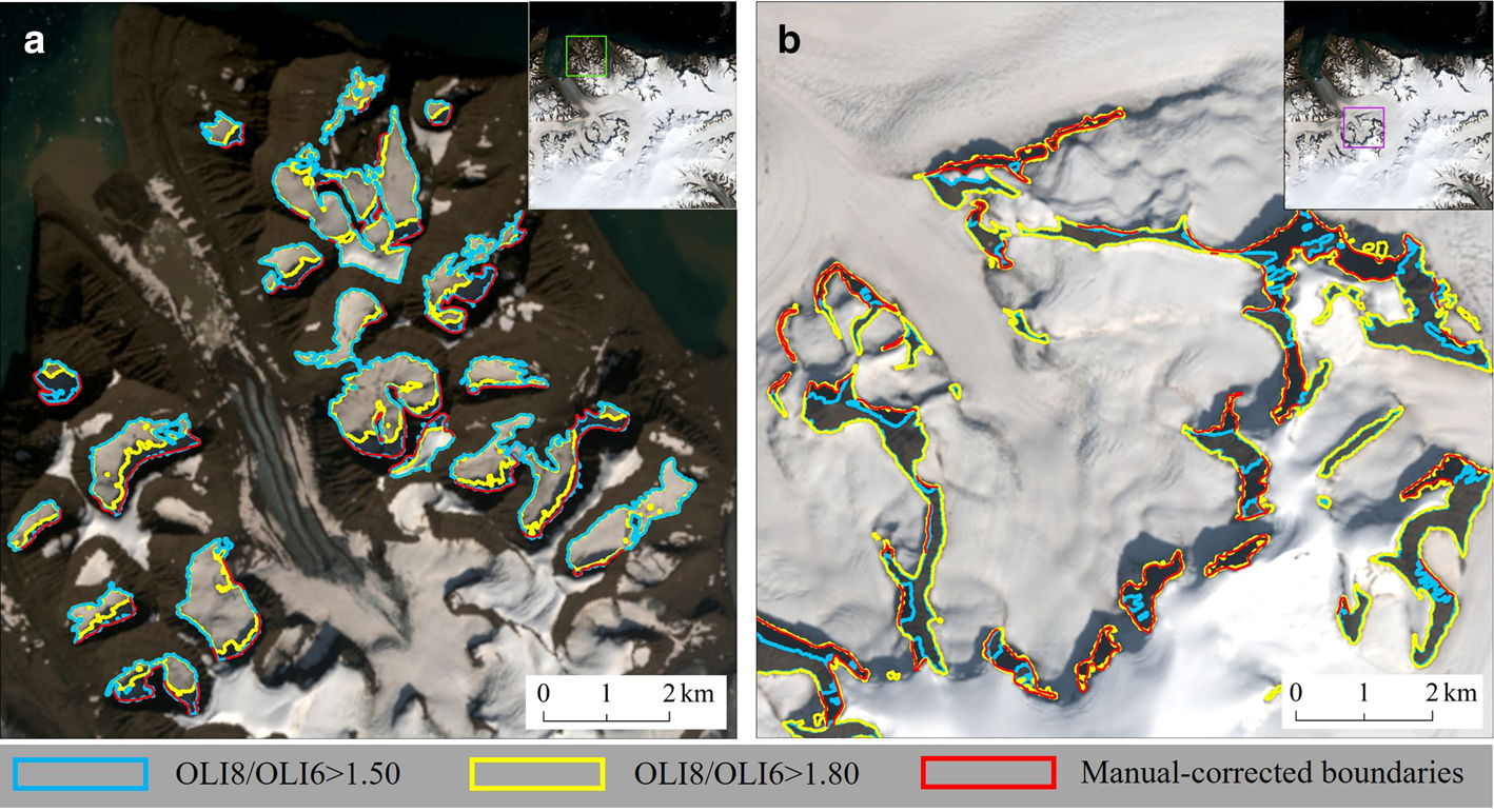
Shaded glaciers were effectively corrected by increasing the brightness of the optical images. Coherence images also assist in mapping glaciers in deep shadow when using slope thresholds to exclude low coherence due to steep mountain slopes. In scheme 1, OLI band ratio reduces workload by providing accurate mapping in the shaded areas without the need to add a threshold in the blue band (Paul and others, Reference Paul, Winsvold, Kaab, Nagler and Schwaizer2016). However, when the image ratio is applied to a scene with larger coverage and more complex terrain, mapping of ice in shadows remains limited because a single threshold is insufficient to map shaded ice in both dark zones and slightly brighter zones. The latter appears brighter because it is on a broad snowfield in high terrain, with surrounding snow in sunlight creating diffuse reflection (Paul and others, Reference Paul2017), whereas the former is generally in low-lying terrain and blocked by steep mountains. Accurate mapping of shaded ice in bright zones requires a high threshold for the OLI8/OLI6 ratio, while shaded and dirty ice in dark zones requires a low value (Fig. 4). Similarly, mapping of brightly shaded rocks requires a higher upper blue reflectance threshold than shaded rocks in darker areas in scheme 2. In this case, we alternately selected thresholds for accurately mapping shaded ice in dark or light zones even in a single scene. We manually created masks that could distinguish between bright and dark zones and separated them at locations where the classification results are insensitive to the threshold. These masks were used to crop one of the ratio images and mosaic the result over the other ratio image. The selection of masks and thresholds, depending on the actual scene, is always an optimization process and a trade-off between total amount of manual correction required for the range. We performed this work before converting the classification raster into a vector. The process of distinguishing between bright and dark scenes also takes time but could reduce the need for extensive corrections to the vectors.
Shaded ice requires different thresholds for the OLI8/OLI6 ratio in dark and bright zones. The glacier scene is located in CE of Greenland (70.2$^\circ$ N, 25.0$^\circ$
 W). (a) A low threshold (1.50) produces better results than a high threshold (1.80) for automatic mapping of shaded ice in dark zones. (b) A high threshold leads to better results than a low threshold for automatic mapping of shaded ice in bright zones. Correct glacier boundaries were indicated manually at the difference between them (regardless of the debris-covered ice), which generally cover blue boundaries in (a) and yellow boundaries in (b), respectively.
In the absence of fieldwork, identifying ice-debris complexes (including rock glaciers, ice-cored moraines and debris-covered dead-ice bodies; Bolch and others, Reference Bolch, Rohrbach, Kutuzov, Robson and Osmonov2019) gives a great challenge to glacier interpreters, such as separating them from bedrock and flowing debris-covered glaciers. Another problem is that there is currently no clear definition of the characteristics that should be included in a glacier inventory. When earlier inventories blur these definitions, updating and creating glacier outlines becomes more difficult (i.e. interpretation differences must be considered). In previous work, Paul and others (Reference Paul, Huggel and Kaab2004) specified how debris cover should be handled during glacier mapping. Molg and others (Reference Molg, Bolch, Rastner, Strozzi and Paul2018) followed a more conservative interpretation when no clear boundary between debris-covered glaciers and rock glaciers could be found. In this study, we chose to exclude rock glaciers, bedrock and stable moraines without ice core melting or significant surface collapse from the inventory. We primarily rely on coherence information to categorize debris-covered glaciers and moraines that show signs of activity as glaciers, and refer to them collectively as debris-covered glaciers.
The debris covering a glacier has the same spectral properties as the surrounding terrain (Paul and others, Reference Paul, Huggel and Kaab2004), meaning that the application of automatic delineation methods would lead to misclassification. We therefore combine optical images and coherence maps to map debris-covered glaciers. On a false-color composite (RGB in bands 654, respectively) of OLI images, debris cover typically shows a darker brown color than the surrounding land. In addition, typical features of debris-covered glaciers, such as distinctive tongues and the presence of melt water streams and small melt water ponds, contribute to their identification (Howat and others, Reference Howat, Negrete and Smith2014). Coherence images provide an accurate reference for mapping the edges of glacial tongues, either as raw images or with added coherence or slope thresholds (e.g. Atwood and others, Reference Atwood, Meyer and Arendt2010; Frey and others, Reference Frey, Paul and Strozzi2012; Ke and others, Reference Ke2016; Lippl and others, Reference Lippl, Vijay and Braun2018). However, there is an uncertainty in discerning debris-covered glaciers by coherence in potentially changing landforms such as snow cover (Molg and others, Reference Molg, Bolch, Rastner, Strozzi and Paul2018), so decorrelation on debris-covered glaciers must be separated from that caused by changes in the surrounding land cover (Barella and others, Reference Barella2022). Therefore, the land cover type was first determined from multi-time and high-resolution optical images (e.g. Nuimura and others, Reference Nuimura2015), and then changes were excluded as much as possible based on the optical images near the timestamp of the interference pair, which is a judgmental process. In some cases, when preliminary estimates of glacier extent are made from glaciological relationships, a tiny accumulation area may not yield a large glacial tongue (Molg and others, Reference Molg, Bolch, Rastner, Strozzi and Paul2018). Moreover, reexamining previous inventories and their source images can provide important references.
Rock glaciers are typically permafrost creep features with high debris content, moving downslope by a few centimeters to a few meters per year, and may originate from ice-cored moraines or be located on talus slopes that provide a continuous debris input (Haeberli and others, Reference Haeberli2006; Berthling, Reference Berthling2011; Monnier and Kinnard, Reference Monnier and Kinnard2015; Molg and others, Reference Molg, Bolch, Rastner, Strozzi and Paul2018). However, the investigation of rock glaciers in Antarctica and Greenland is inadequate and limited to small regions (Rudolph and others, Reference Rudolph, Meiklejohn, Hansen, Hedding and Nel2018; Abermann and Langley, Reference Abermann and Langley2022) and previous inventories do not provide any information on the separation of rock glaciers from glaciers. It is difficult and highly subjective to distinguish rock glaciers from similar features, such as debris-covered glaciers and ice-cored moraines in 30 m spatial resolution images or even in high-resolution images (Janke and others, Reference Janke, Bellisario and Ferrando2015; Paul and others, Reference Paul2017; Reinosch and others, Reference Reinosch2021). Line-of-sight (LOS) surface velocity estimation from InSAR has been applied successfully to determine rock glacier activity in regional inventories in recent years (Villarroel and others, Reference Villarroel, Beliveau, Forte, Monserrat and Morvillo2018; Strozzi and others, Reference Strozzi2020; Brencher and others, Reference Brencher, Handwerger and Munroe2021; Reinosch and others, Reference Reinosch2021; Zhang and others, Reference Zhang2021). However, InSAR suffers from limitations closely related to rock glacier studies, including underestimation of true 3D velocities, decorrelation arising from changing surface properties, atmospheric delay and the maximum detectable displacement between two SAR acquisitions (Villarroel and others, Reference Villarroel, Beliveau, Forte, Monserrat and Morvillo2018; Brencher and others, Reference Brencher, Handwerger and Munroe2021; Reinosch and others, Reference Reinosch2021). Mitigating these problems requires careful study designs and a considerable amount of work. In addition, it remains difficult to define indicators to distinguish rock glaciers from debris-covered glaciers because they may have similar rates of movement (Villarroel and others, Reference Villarroel, Beliveau, Forte, Monserrat and Morvillo2018). Unlike debris-covered glaciers with longitudinally flowing ridges and distinct lateral and central moraines, rock glaciers tend to exhibit pronounced transverse ridges and furrows perpendicular to flow direction, showing lobate (width-to-length ratio ≥1) or tongue-shaped (width-to-length ratio <1) forms (Janke and others, Reference Janke, Bellisario and Ferrando2015; Tanarro and others, Reference Tanarro, Palacios, Zamorano and Andres2018; Strozzi and others, Reference Strozzi2020). Therefore, we excluded rock glaciers by using high-resolution images to identify landforms and the morphology of debris accumulation on the glacier surface. When high-resolution images are missing and difficult to judge, we relied on coherence images for mapping because it helps to exclude at least inactive rock glaciers, but may result in an overestimation of debris cover.
3.2 Delineation of glacier divides
The next step in creating a glacier inventory is to separate glacier complexes based on hydrologic divisions, and the location of the divides determines the number and area of individual glaciers (Paul and others, Reference Paul, Kääb, Maisch, Kellenberger and Haeberli2002; Ke and others, Reference Ke2016). Racoviteanu and others (Reference Racoviteanu, Paul, Raup, Khalsa and Armstrong2009) recommended that ice divides should be placed in the same location as in previous inventories when comparing glacier extents. However, previous inventories used early DEMs as input for watershed analysis, and their vertical accuracy and resolution is inadequate compared to recently published DEMs (see section 2.3). Inaccurate and coarse DEMs can lead to topographic divisions that differ from the true topographic divides, ultimately resulting in shifted glacier divides (Kienholz and others, Reference Kienholz, Hock and Arendt2013).
We referred to the semi-automatic method of Bolch and others (Reference Bolch, Menounos and Wheate2010) and Kienholz and others (Reference Kienholz, Hock and Arendt2013) to create buffer zones around each glacier complex. This method can be used for any time period and extent (Bolch and others, Reference Bolch, Menounos and Wheate2010) and is very conducive to splitting glaciers with significant topographic variation in the accumulation zone (e.g. protruding rock ridges or summits). We clipped the DEM to the buffer zones and calculated the glacier basins using watershed analysis tools in ArcGIS. Basins were created automatically by locating pour points and depressions at the edges and determining the convergence area of each pour point. We subsequently converted the calculated basin raster into polygons representing the glacier basins. These polygons were merged to clip the glacier complexes supported by aspect and ice velocity maps, and with reference to the merging rules of the previous inventories. However, potential DEM artifacts in the accumulation zone can lead to errors in the automatically derived ice divisions (e.g. Bolch and others, Reference Bolch, Menounos and Wheate2010; Ke and others, Reference Ke2016) and significant uncertainty in demarcating glaciers in areas of flat accumulation that lack distinct topographic features to support visual judgments. Therefore, we manually corrected the watershed by combining color-coded flow-direction grids in the background (e.g. Paul and others, Reference Paul, Frey and Le Bris2011), hillshade maps, optical scenes and ice velocity maps to reduce the error. Finally, sliver polygons created by the intersection of watersheds with glacier boundaries due to the possible differences between the DEM used for the orthorectification of the optical image and the DEM used to derive ice divides were checked and manually corrected.
Separating glaciers among ice fields is quite challenging in the study area. A large outlet glacier may originate from numerous interconnected valley glaciers or the ice sheet upstream, which increases the difficulty of assigning glacier extent. The divisions used in the previous inventories were useful in reducing the effort to trace accumulation areas of the glacier. Importantly, we checked and adjusted the extent of individual glaciers based on the ice velocity map. As in the previous inventory, to divide a very large glacier in intricate terrain, some glacier divisions were added even though they lack support information.
In Greenland, the watersheds generated by Rastner and others (Reference Rastner2012) based on the GIMP DEM were used not only to define glacier divisions, but also as connections between the GIC and the ice sheet, with CLs defined as weak (CL1) and strong (CL2). Here, another challenge occurred: the position of these boundaries changed when the watersheds were generated from a new DEM, either considering real topographic variations or the effect of different vertical accuracy and resolution of the DEM. Secondly, the separation of the GIC from the ice sheet in the previous inventory is necessary, while the merging of basin polygons and glacier divisions here can be very subjective and straightforward (accumulation areas that contribute to glacier flow may not be included in the GIC). Therefore, we decided to retain the watersheds generated by Rastner and others (Reference Rastner2012) using GIMP DEM where glaciers are connected to the ice sheet and use new watersheds to divide the glacier complexes. The reasons for this are: (1) RGI 6.0 has been used in many existing studies; (2) the difference in watersheds derived from the GIMP DEM and the ArcticDEM is acceptable (see section 5.3); (3) the inconsistency in glacier definition due to artificial factors and differences in accuracy of DEM can be avoided; (4) this provides advantages in time series analysis of glacier change; and (5) glacier area generally changes very little at the internal basin boundaries with the ice sheet even when surface elevation changes.
3.3 Assignment of glacier attributes
To complete the glacier inventory, the necessary fields such as source date, glacier area, minimum, maximum, median and mean elevations, mean slope and aspect, and CLs were created for each glacier outline. For the same glacier mapped with multiple images, the last acquisition date of the images was taken as the as-of-time (i.e. source date; GLIMS Analysis Tutorial, https://www.glims.org/MapsAndDocs/guides.html). In this work, glacier areas were calculated using the South/North Pole Lambert Azimuthal Equal Area coordinate system. Attributes of glacier-specific topographic parameters (e.g. elevation, slope and aspect) were calculated by combining the glacier outlines with the topographic raster using the zonal statistics tool in ArcGIS. This tool statistically summarizes the values of the topographic raster dataset within the glacier outline zone and links the results to the glacier outline attribute table using a common and unique identifier (i.e. the glacier ID).
In Greenland, glaciers classified as CL0 have no connection with any other class, CL2 glacier complexes have a relatively stable boundary in contact with the ice sheet and CL1 glacier complexes may have contact with the ice sheet in the accumulation or ablation zones. Glaciers in contact with the ice sheet are assigned CLs first. Due to the ‘topological heritage’ rule, the connected entities (in the glacier complex) of glaciers that have been assigned CLs also adopt the same class (see Rastner and others, Reference Rastner2012), so that the CLs of a set of entities can be co-varying. However, changes of individual glaciers are difficult to describe systematically, for example: some local glaciers may have disappeared and individual glaciers may have changed due to glacier division shifts; glaciers that were originally part of a glacier complex may have separated due to ablation, especially where the topography is prominent and originally divided by a watershed; and glacier tongues that retreated in the ablation zone lost contact with the ice sheet. All of these may lead to a change in CLs of glaciers with the ice sheet from high to low. Therefore, we emphasize that the CLs of Greenland glaciers need to be checked again.
4. Application and results
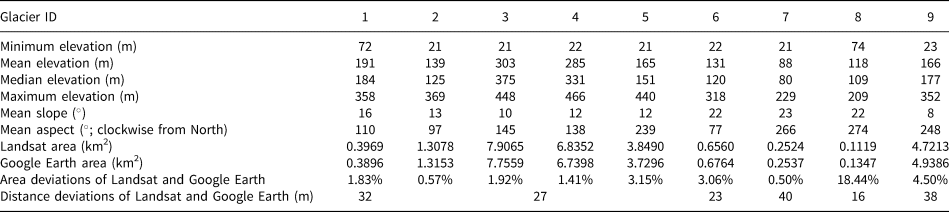
In this section, we present and discuss the application and results of updating glacier outlines in representative areas of Antarctica and Greenland following our approach outlined in the methods. We take James Ross Island (this case gives glacier attribute samples; Table 1), Ross Island and the region around Kangerlussuaq Fjord as application cases (Fig. 1). The updated glacier outlines were overlaid on the background images and compared qualitatively with the previous inventories. Watersheds are difficult to compare because they are affected by the date (thus need to take into account glacier and terrain changes) and accuracy of the DEM (Kienholz and others, Reference Kienholz, Hock and Arendt2013). In addition, the rules for merging basins are not always consistent due to different processing procedures. The ability of watersheds generated from DEMs of different periods to reflect the true glacial topographic divisions during the corresponding periods in areas of weak glacial and topographic variability is discussed in section 5.3 with examples.
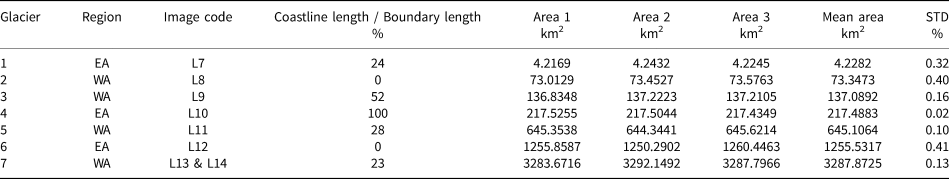
Attribute examples of CL0 glaciers (1–9 in Fig. 6) with source date of 23 Dec 2021 and deviations between Landsat and Google Earth results
Due to the lack of ground truthing, we quantitatively assessed the uncertainty or precision of the updated glacier outlines, rather than the accuracy (Paul and others, Reference Paul2017; Molg and others, Reference Molg, Bolch, Rastner, Strozzi and Paul2018). For glacier boundaries, the uncertainty or precision is determined in two different ways: in the case of automatically derived boundaries, values were taken from the literature or manual digitization results based on the same images were compared; in the case of manually digitized or improved boundaries, the results of mapping based on higher-resolution images are used for cross-validation. However, problems with high-resolution imagery in Google Earth, including different source date, small spatial coverage, potential snow, cloud and shadow conditions, and the quality of DEM used for orthorectification, limit its ability to be used as reference data (Paul and others, Reference Paul2017). We mitigated these influences by selecting high-resolution images with close timing to the used Landsat images and better mapping conditions (e.g. less cloud and snow cover) and geographic registration accuracy. We also assessed the precision of glacier divides based on light and dark divisions in the background images or by comparison with the results of visual interpretation at clear topographic divides.
4.1 Case study 1: James Ross Island
Glaciers on James Ross Island terminate on land or in the ocean, and can be covered in debris that is uncommon in other parts of Antarctica. These glaciers are considered to be ice caps and not divided by watersheds (Bliss and others, Reference Bliss, Hock and Cogley2013).
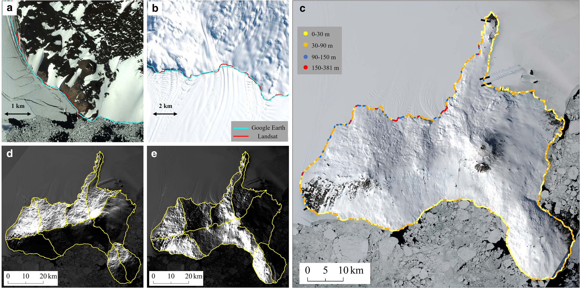
The OLI8/OLI6 ratio image (L1) includes more shaded ice in dark zones at a threshold of 1.51 and a higher threshold of 1.85 was applied for brighter bare rock and shadows (Fig. 5a). We cropped ratio images to a buffer (1 km) of the REMA contour at the edges of the island (25 m) to reduce the processing efforts and manually corrected the automatically derived boundaries (Figs 5b, c). Raw and threshold coherence images and optical images were used together to reduce the selection omission of ice pixels. Using multi-time images (1988, 2000, 2015 and 2021) and high-resolution images in Google Earth, land cover types such as snow and debris cover were discriminated and mapping challenges were addressed. We primarily used the C1 coherence image and the optical images near the time of interference pairs to exclude coherence loss which probably occurred due to snowfall and melting (Figs 5d, e). Possible snow or ice cover that matches the irregular shape features and shows higher coherence (>0.4) was regarded as snow and excluded. The decision process was also supported by a combination of five additional coherence maps (C2–C6) with different time baselines and the previous inventory.
Application case of the methods for James Ross Island in AP. (a) Glacier scene (L1, 20211223) with updated glacier outlines (yellow). The blue and red boxes correspond to the scene subsets (b, d, f) and (c, e, g), respectively. White represents the buffer (1 km) zone of the REMA contour (25 m). A higher OLI8/OLI6 ratio threshold (1.85) was used within the created masks (black). (b, c) Selected examples of the correction to the raw classification results (white). (d, e) The use of threshold coherence map (C1, 20211212-20220204; a 3 × 3 low-pass filter was applied to smooth boundaries) to support glacier mapping. The left insets provide a further view of the optical images near the time of interference pairs for the blue and red boxes in (a). The black arrows in (b, d) indicate that coherence loss due to snowfall is excluded when plotting glaciers and in (c, e) indicate that the exclusion of snow or ice cover that matches the snowpack features and shows higher coherence. (f, g) Comparison of updated glacier outlines with RGI 6.0 (purple). The white arrows indicate where the updated glacier outlines and RGI 6.0 differ in terms of debris and snow cover.
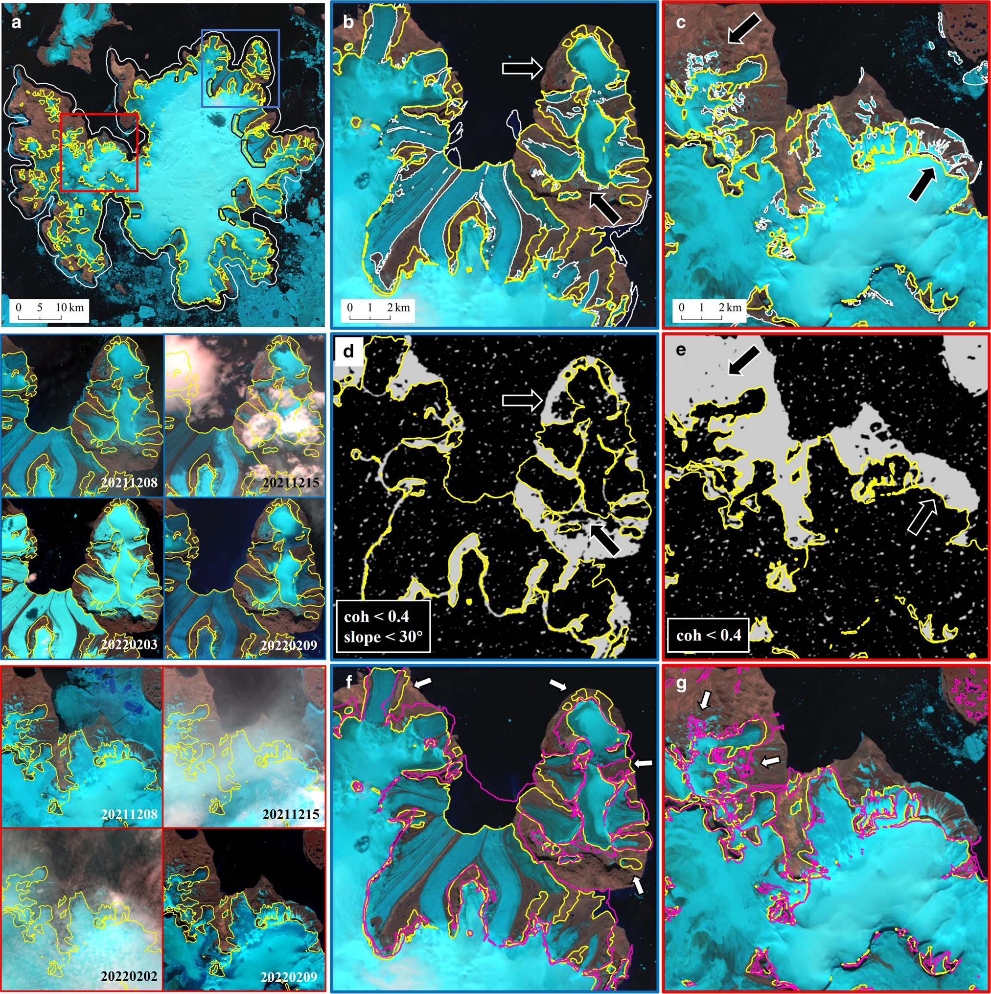
The overlay of outlines shows the corrections to the automatically derived glacier outlines (Figs 5b, c), and explains the differences with the previous inventory (Figs 5f, g). Some differences were carefully examined in high-resolution images from Google Earth and did not create ambiguities. Previous and updated glacier outlines are able to correctly represent most of the clean ice from the corresponding period. However, excluding factors of glacier variability and outline positioning accuracy creates large differences in the interpretation of debris and snow cover. From the assessment factors of the Third Pole inventories by He and Zhou (Reference He and Zhou2022), the medium- to high-resolution scenes, unstriped imagery and less snow and shadows, as well as the combination with InSAR technique, are favorable to reduce uncertainty in the process of updating glacier outlines here.
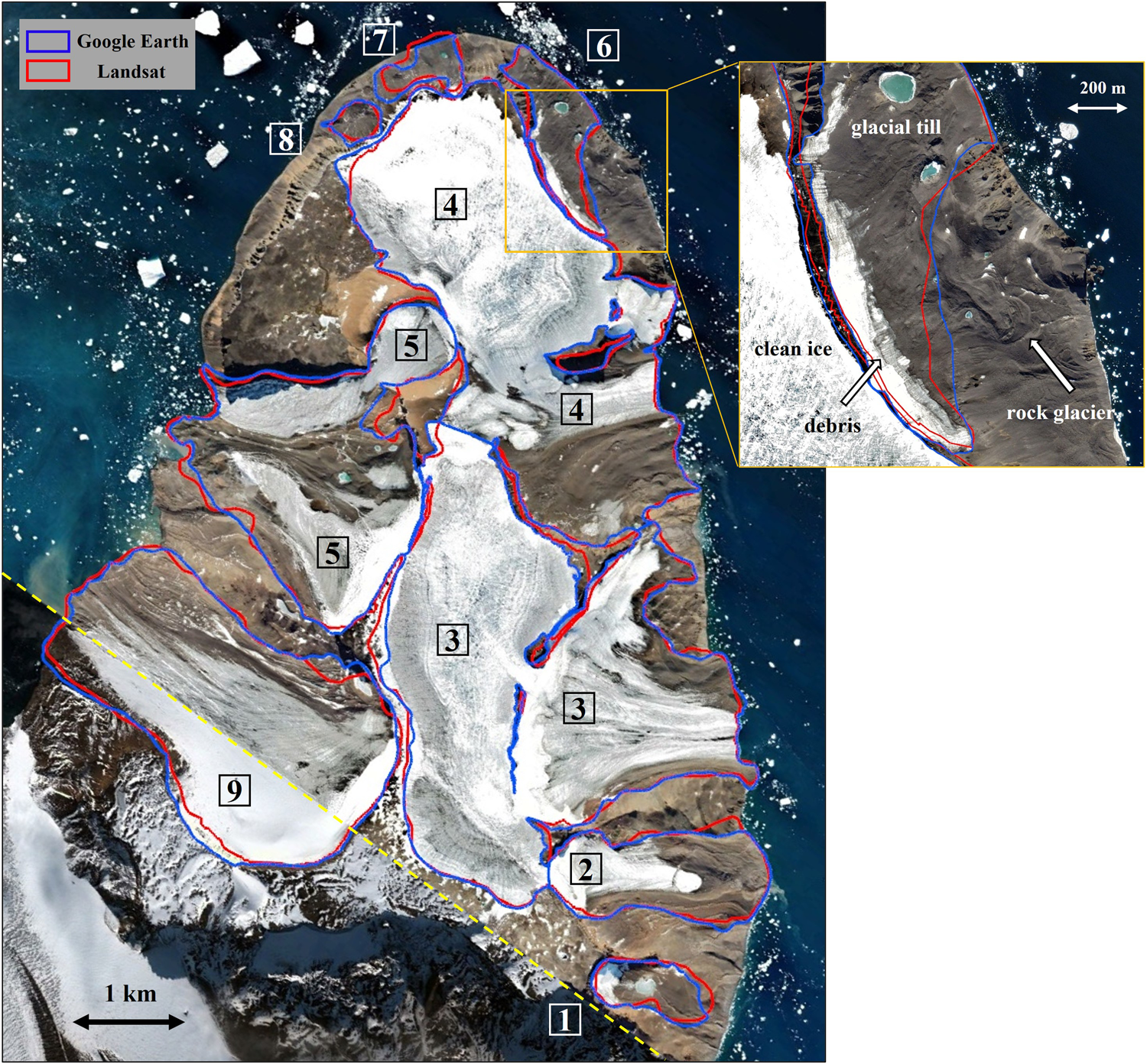
Automatic mapping of clean glaciers is at least as accurate as manual digitization, or has only single-pixel differences (Paul and others, Reference Paul2013). As shown in Figure 6, we depicted nine debris-covered glaciers based on high-resolution images in Google Earth with close timing to a Landsat image (L1, 20211223) and calculated their area deviations. The calculated area deviation value in Table 1 tends to increase toward larger glaciers (e.g. Paul and others, Reference Paul2013, Reference Paul2017), so it is inappropriate to apply these percentages for the entire glacier area. As in many studies (e.g. Granshaw and Fountain, Reference Granshaw and Fountain2006; Bolch and others, Reference Bolch, Menounos and Wheate2010; Rastner and others, Reference Rastner2012), the glacier buffer approach was used to calculate the relative change and estimate the uncertainty in glacier size. The mapping results from Google Earth were converted from KML to SHP, which can be loaded into ArcGIS and then compared with Landsat boundaries. Points were taken every 30 m along the Landsat boundary and their distance from the nearest points on the corresponding Google Earth boundary was calculated (this method is referred to as the nearest neighbor method in the following sections; e.g. Guo and others, Reference Guo2015). Glaciers have an average distance deviation of about 1 pixel or 30 m between the two boundaries (Table 1). Applying this deviation to the buffer method, we obtained an uncertainty of 2.4% in the mapped glacier area of James Ross Island.
Overlay of boundaries of nine glaciers (1–9) on James Ross Island mapped using Google Earth and Landsat, with a high-resolution screenshot from Google Earth. The upper scene (17 Jan 2021) and the small scene below (18 Mar 2009) are separated by the yellow dash line. The center glacier complex was divided based on 3D views in Google Earth to facilitate comparison of glacier areas. The right inset shows an ice-debris landform and the features of the moraine deposits here are consistent with ice-cored moraine characteristics described by Strelin and Sone (Reference Strelin and Sone1998) and buried glaciers described by Janke and others (Reference Janke, Bellisario and Ferrando2015), including appearance of pockmarks, ponds and weak development of surface ridges. Please note the coherence information at the corresponding location on the right side in Figure 5d. It is difficult to accurately separate rock glaciers even in Google Earth because they have obscure transitions with debris-covered glaciers.
4.2 Case study 2: Ross Island
The majority of the glaciers containing glacier watersheds on Ross Island are marine-terminating, either with ice shelves or connected to sea ice at the margin, and a small number are land-terminating.
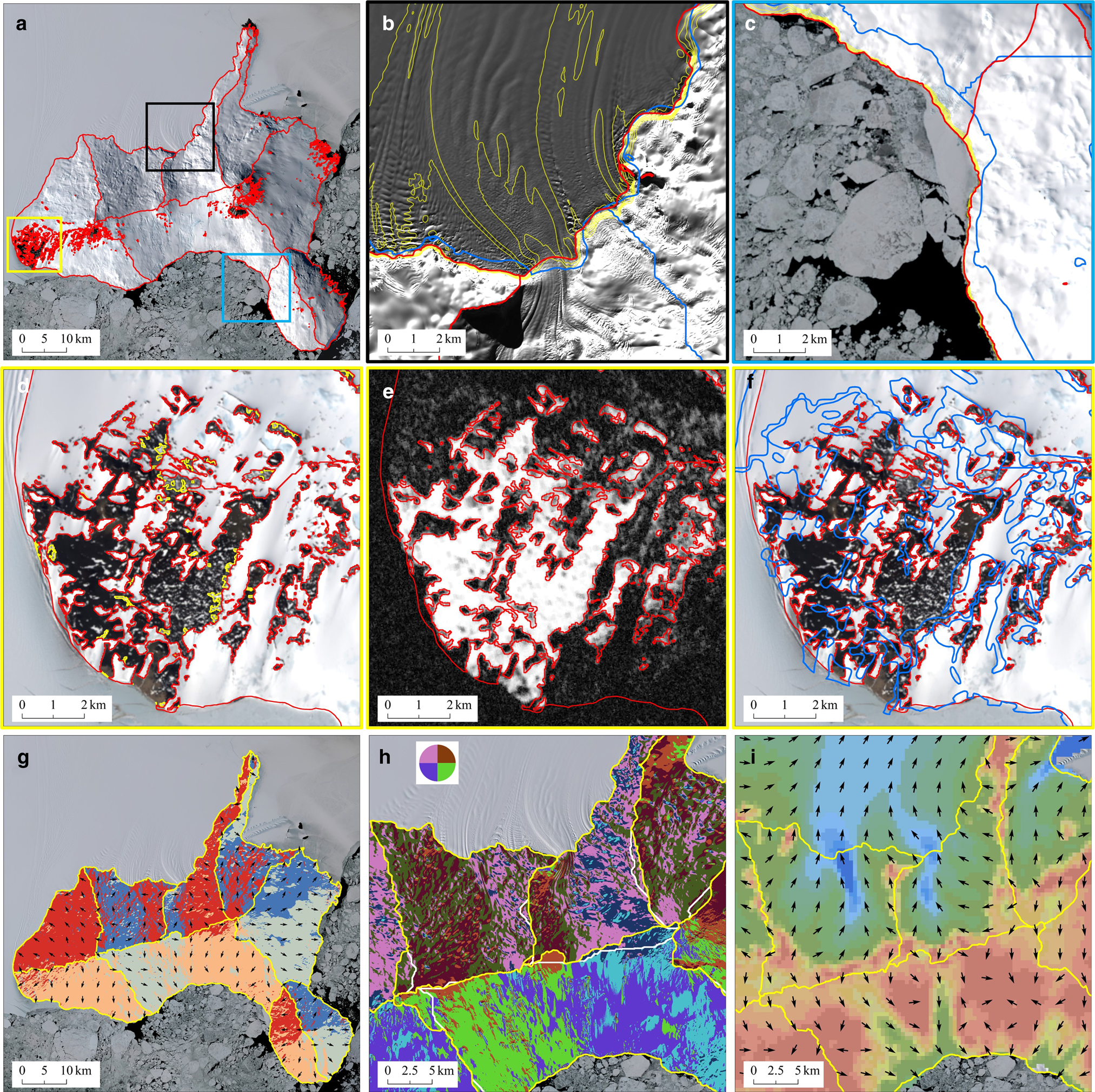
Three images from 2018 (L2–L4) with various enhancements served as inputs for mapping the glacier boundaries. REMA was used to generate contours for providing a reference for image-based manual digitization of glacier boundaries (Figs 7b, c) and create watersheds following the method described (Figs 7g–i). In most cases, the land-terminating glacier boundaries were not mapped manually, but were obtained by excluding rock outcrops within the mapped outer boundary (i.e. the outermost edges of the island are regarded as the glacier outer boundary; Figs 7d–f). The raw images (L2) were processed in ENVI to obtain TOA reflectance corrected and brightness-temperature converted data. The glacier outer boundary mask and a set of thresholds were used to produce the rock outcrop raster (NDSI >0.7, blue <0.32 (a single blue threshold is sufficient to map this scene with more consistent shading conditions), TIRS1/blue >400, TIRS1 >255 K). Six coherence images (C7–C12) with a stack of their minimum values and additional Landsat scenes (2001, 2014 and 2019) were used to view snow conditions and support the modification of snow-covered rock areas (Fig. 7e). The rock outcrop vectors were intersected with the glacier outer boundary and watersheds to derive outlines of Ross Island glaciers (Fig. 7a).
Application case of the methods for Ross Island in EA. (a) Glacier scene with updated glacier outlines (red). The black, blue and yellow boxes, respectively, correspond to the scene subsets (b, c) and (d, e, f). (b, c) Selected examples of ice-shelf-terminating and marine-terminating outer boundary mapping, respectively, with (enhanced) images and contours (yellow; −30, −15, 0, 15, 30 m) generated from REMA. Glacier outlines from RGI 6.0 are shown in blue. (d) Selected example of the correction to the raw rock classification results (yellow) at the snow cover. (e) Minimal composite from six coherence images (C7–C12) helps exclude blurred snow patches around glaciers. Dark color indicates areas of low coherence. (f) Comparison of updated glacier outlines with RGI 6.0 in rock area. (g) The intersection (yellow) of glacier outer boundary and watersheds with an aspect map. (h) Correction to the raw watersheds (white) with the help of the color-coded flow-direction grid. (i) Direction and magnitude (blue>green>brown) of ice velocity guide the delineation of glacier divides.
When updated glacier boundaries and those in RGI 6.0 were overlaid for comparison, significant positioning and generalization differences can be observed (Figs 7b, c, f). Actually, glacier boundaries in the previous inventory by Bliss and others (Reference Bliss, Hock and Cogley2013) were derived primarily from polygon files from ADD 3.0, which were manually created based on sources with various resolutions and accuracies (e.g. paper maps, aerial photographs and optical images). The previous rock dataset has some significant georeferencing inconsistencies, misclassifications and overestimation of Antarctic ice-free areas (Burton-Johnson and others, Reference Burton-Johnson, Black, Fretwell and Kaluza-Gilbert2016). Therefore, the accuracy of this inventory is regionally inconsistent and without associated quality assessment. In our work, the original data sources are from the Landsat L1 T dataset (see section 2.1), which includes accurate geographic calibration and orthorectification using digital topography (Wulder and others, Reference Wulder, Masek, Cohen, Loveland and Woodcock2012). As a result, the updated glacier boundary is of high global positioning accuracy. We used elevation references from REMA in addition to planimetric imagery to reduce the subjectivity of mapping glacier boundaries. The classification accuracy of Burton-Johnson and others (Reference Burton-Johnson, Black, Fretwell and Kaluza-Gilbert2016) method for rock pixels is 74 ± 9% and is more accurate and consistent than the ADD rock dataset (only 39 ± 19%) (see Burton-Johnson and others, Reference Burton-Johnson, Black, Fretwell and Kaluza-Gilbert2016), so the improvement in rock classification accuracy is significant.
We used Google Earth with the excellent 3D rendering and high-resolution images to help assess the precision of manually mapped glacier outer boundaries. In the mapping process, the image at 30 m resolution (Dec 2018) was used as the primary reference. In areas with less intense glacier variability, images with a resolution of less than 1 m from different years (2011, 2012, 2015, 2017 and 2021) were also referenced to provide a finer representation of the boundaries (Fig. 8a). The glacier boundary, which was drawn based on images from different years, was checked for matches with the Dec 2018 image and adjustments were made. The 3D terrain height display in Google Earth was expanded threefold to better visually represent the boundary between glacier and ice shelves (Fig. 8b). We used the nearest neighbor method to calculate the deviation from the Google Earth boundary for every 100 m of sampling points on the Landsat boundary (Fig. 8c). The results show that the overall average deviation is about 32 m, the average deviation of the boundary between glaciers and ice shelves (including the glacier outlet) is about 58 m, and for the boundary between glaciers (or island) and the ocean (including very few land-terminating boundaries) the average deviation is about 20 m. Most of the deviations above 90 m occur at the glacier outlet and the boundary between glaciers and ice shelves. The difference in area enclosed by the two sets of glacier boundaries was calculated, and the results show that the area derived using Google Earth is approximately 0.11% larger than that derived from Landsat images using our approach.
Precision assessment of glacier outlines on Ross Island. (a, b) Two examples of precision assessment of glacier outer boundaries on Ross Island. Blue indicates boundary mapping using high-resolution image (30 Dec 2011) and using 3D view (Dec 2018) from Google Earth, respectively. Red represents the boundary mapped based on Landsat images. (c) Deviations between Landsat and Google Earth boundaries. The black truncated lines indicate the boundary division of ice shelf terminus and ocean terminus. (d) (e) The intersection of glacier outer boundary and watersheds and two stretched images (L2, L3) with sun azimuths near perpendicular to each other.
We used a method that considers the length of the glacier boundary and its positioning accuracy to assess the total area error of glaciers on Ross Island (Rivera and others, Reference Rivera, Bown, Casassa, Acuna and Clavero2005; Guo and others, Reference Guo2015). The evaluation of the glacier area error is calculated from the following equation:

where EA is the glacier area error, L1, D1, and L2, D2 are the length and average deviation of ice-shelf-terminating and marine-terminating glacier boundary, respectively, and AR is the total area of rock outcrops, obtained by subtracting the area of final glacier outlines from the area of the outer glacier boundary. The rock classification accuracy was considered to be 74% and the value of 0.26 was used as the factor for the rock area error term. Manual corrections were made to the automatically derived rock classification results, so this is an upper bound estimate. It is shown that the glacier area error contributed by the glacier outer boundary is 0.44% and by the total rock area is 1.14%, so the total area error is 1.58%.
The watersheds generated using REMA perform well and the stretched images were used as background for examining the watersheds. As shown in Figures 8d, e, the watersheds are able to match the light and dark divisions in the stretched images well. Visual checks of watersheds at clear topographic divisions in the image show average deviations that are about one pixel (32 m).
4.3 Case study 3: Kangerlussuaq Fjord
The study area with GIC of all CLs around Kangerlussuaq Fjord has different local lighting conditions due to the complex terrain and contains clean or dirty ice, shaded ice and more debris-covered ice.
Three median-filtered OLI8/OLI6 ratio images of the same OLI scene (L5) were cropped and mosaicked to map glaciers with varying local illumination conditions in this region: an OLI8/OLI6 threshold of 1.75 was used for bright snowfields on high terrain, and low thresholds of 1.35 and 1.50 were used to map dark zone glaciers on low-lying terrain near the coast (Fig. 9a). Boundaries between GIC and the ice sheet from the previous inventory were retained (Figs 9b, c) and misclassified boundaries were manually improved (Figs 9d–f). To address the challenges of snow, debris cover and shadows in this scene, another image from a close time (L6) was used and multi-temporal images (2000, 2002 and 2019) were viewed alternately. Two of the better coherence images (C13–C14) were used as the primary references and the rest (C15–C18) were used as supplementary references. The low consistency due to steep slopes in this complex terrain reduces the usability of raw coherence maps, so slope thresholds were selected and applied. We then used the ArcticDEM and watershed analysis tools to create the watersheds, modified and added some necessary divisions based on the flow-direction raster, optical images and ice velocity map (Figs 9g–i).
Application case of the methods for the region around Kangerlussuaq Fjord in CE Greenland. (a) Different OLI8/OLI6 thresholds were used for the glacier scene (L5, 20140816) to update glacier outlines (yellow), preserving boundaries between GIC and ice sheet from RGI 6.0 (red). The black, blue and green boxes correspond to the scene subsets (b, c), (d, e, f) and (h, i), respectively. (b, c) respectively, explain that the basin raster and the direction of ice flow may not support the demarcation of GIC and ice sheet, which is influenced by artificial factors. (d, e) An example of correction to the raw classification results (white) guided by the optical scene and the threshold coherence map (C14, 20150813–20150906), respectively. (f) Overlay of updated and RGI 6.0 (purple) glacier outlines on the glacier scene (20150828). In (e) and (f), the interference of low coherence due to snow melting at the black arrow was excluded and some snow patches at the white arrows were filtered by the coherence threshold. (g) Dividing glaciers on an intricate ice field with the help of the magnitude (purple>blue>green>brown) and direction of ice velocity. The watershed in the black circle aims to divide a very large glacier, but lacks information to support it. Black are outlines of the overlaid RGI 6.0. (h) The raw merged basin polygons (black), with manually identified dots (white) on the watershed. (i) Final divided glacier extent (blue) in (h), with a hillshade map. The accumulation areas of some glaciers are already separated by ridges without help from watersheds (white boxes in (h, i)).
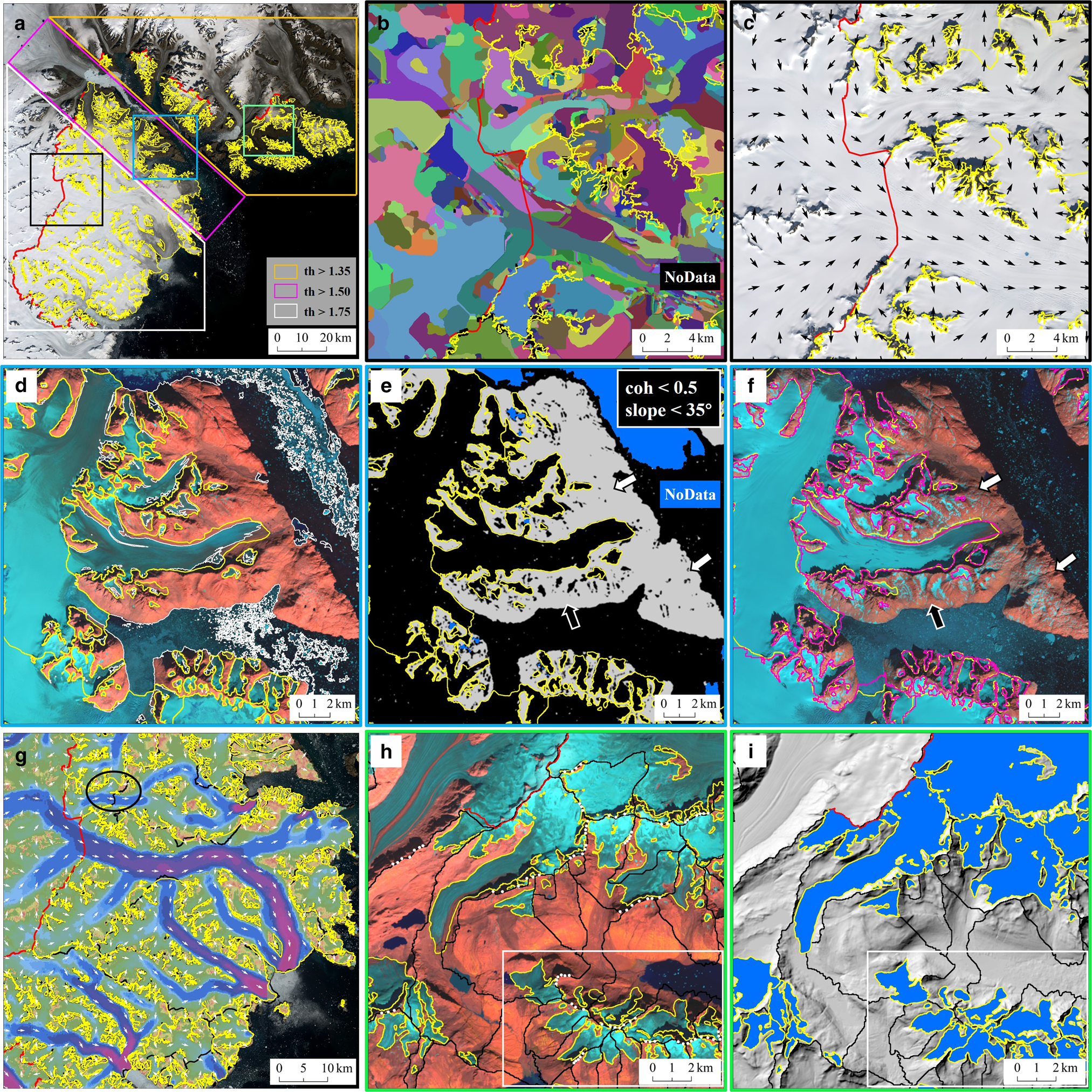
Glacier boundaries mapped by OLI are presented at a higher resolution, so more details are mapped that better reflect the condition and extent of the glacier. Section 5.2 compares the differences in glacier mapping results using OLI and ETM+ at different resolutions. We combined the advantages of mapping shaded ice by OLI with the multi-threshold method to obtain the ice classification results for locally different illumination conditions in a single scene without compromising on threshold selection. As a result, most of the clean and shaded ice in the scene is automatically and accurately drawn, even if they are in areas of different brightness. In particular, few manual improvements are required for rock outcrops mapped in scenes with little seasonal snow, which is useful for mapping glacier outlines containing large amounts of rock outcrops in Greenland.
The precision of glacier boundaries is usually determined by the threshold value for the image ratio and the key is whether the threshold can be satisfied for most areas of the scene, even if some areas (e.g. deep shadows, clouds and debris cover) must be manually improved. A rock outcrop and two representative clean (or slightly dirty) glaciers, which respectively represent the classification results for shaded ice in the brighter zones, ice in sufficient light and shaded ice in dark zones, were manually digitized to compare with the automatic results using the nearest neighbor method (sampling point interval of 10 m on the automatic boundary) and test the applicability of different thresholds to this scene (Figs S1a–S1c). We also depicted three debris-covered glaciers based on images with close timing (26 Jul 2012) in Google Earth and calculated their deviations from the manual Landsat mapping results using the same method (sampling point interval of 10 m on the Landsat boundary; Figs S1d–S1f). Therefore, we used a 15 m buffer around all glacier complexes based on the average of the deviations in Figure S1, and thus calculated the uncertainty of 2.7% for the updated glacier area around Kangerlussuaq Fjord.
The precision of watersheds derived from ArcticDEM was evaluated. With the help of images and Google Earth, we visually identified 90 checkpoints on distinct topographic divides where automatic basin polygon boundaries matched the flow-direction divisions to compare with the raw merged basin polygons (Fig. 9h). The average deviation evaluated using the nearest neighbor method is about 24 m, which is within one pixel of the DEM (32 m).
5. Discussion
5.1 Effects of terminus types on mapped glacier area in Antarctica
In Antarctica, the manually digitized glacier boundaries can be quite long due to the influence of ice shelves and sea ice. The error in identifying glacier boundaries on images varies depending on the terminus type (e.g. Bindschadler and others, Reference Bindschadler2011). The accuracy of boundary mapping is critical for determining glacier area, while the uncertainty of glacier mapping needs to be additionally considered in change analysis. Based on the methodology of this study, we have attempted to assess the effects of terminus characteristics on manually mapped glacier area based on the significance of measured changes in glacier area.
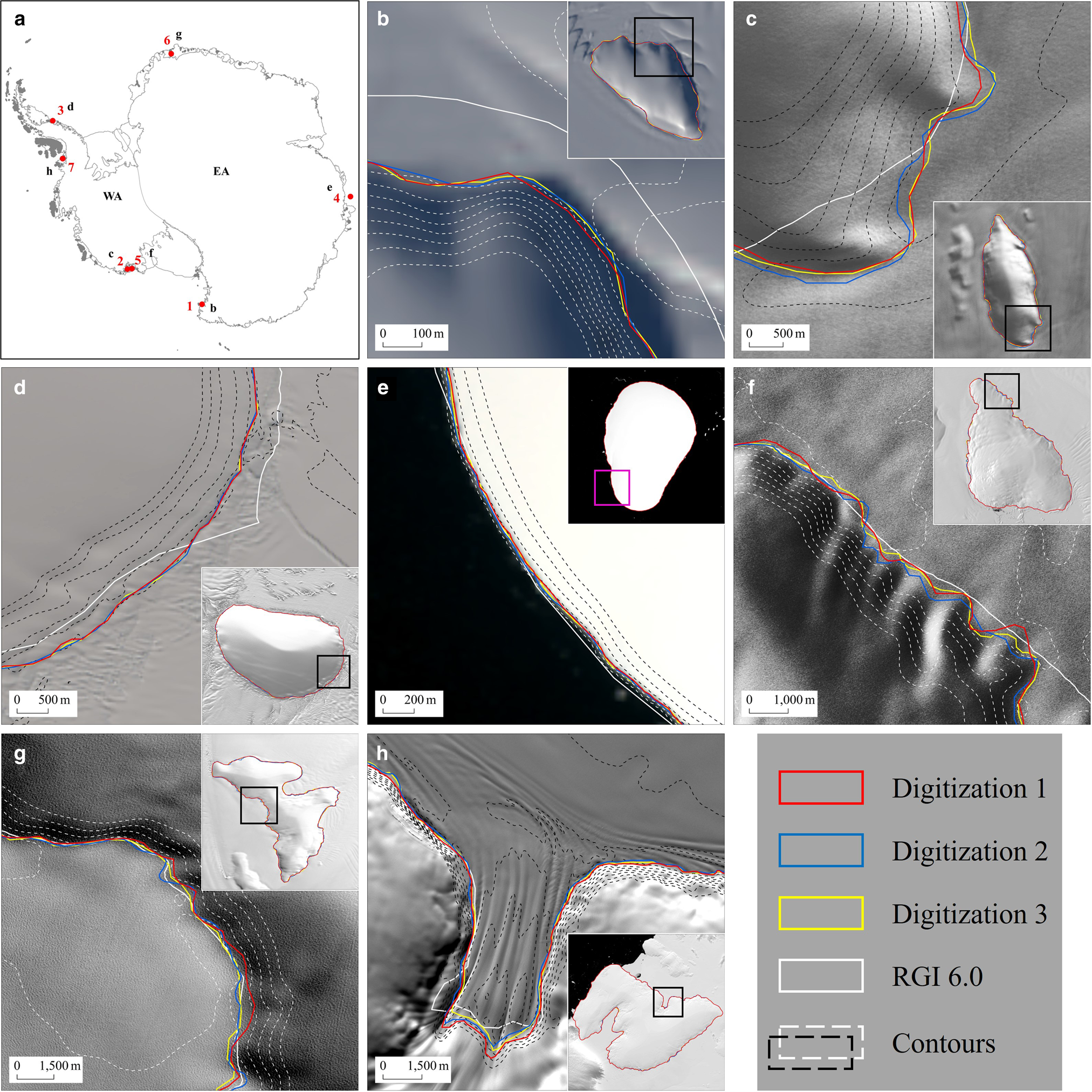
Paul and others (Reference Paul2013) showed the results of their repeated experiments and suggested that glacier outlines should be digitized multiple times and that the average of the results from multiple digitizations is close to the true value. Seven ice caps without rock outcrops in EA and WA were selected (Fig. 10a), so the outer boundaries drawn represent their areas. We digitized their boundaries three times each independently and completed the experimental assessment based on the standard deviation (STD) of these results (Fig. 10). The land-terminating boundary has the same easily distinguishable characteristics as the marine-terminating boundary and thus is not considered. The length of coastline accounts for various proportions of each glacier boundary, and glaciers vary in size and are located in different regions. We then calculated the mean and STD of the triple results for each glacier and show them in Table 2.
Assessing effects of terminus characteristics on mapped glacier areas in Antarctica. Seven glaciers have various sizes and locations, as well as different proportions of ice shelf and marine terminus (1–7 in (a) corresponds to (b)–(h)). Three separate digitizations were performed for each glacier. Contour lines with a contour distance of 10 m were generated from REMA.
Results of digitizing seven glaciers three times and their means and STDs
The results show a maximum STD for glacier area of 0.41% and a minimum of 0.02%. The significance of the change in digitized glacier area does not appear to be related to the area of the digitized glaciers, but is somehow implicitly related to the nature of the boundary and closely related to how easy it is to interpret the glacier boundaries from the images. The area results from multiple measurements become more discrete when the length fraction of the boundaries connected to the ocean in the total boundary is reduced, and conversely it becomes more consistent. Line segments can often be traced to the nearest pixel when mapping glacier boundaries with the ocean (Fig. 10e), but the low contrast between glacier and ice shelf causes many difficulties in defining and identifying some glacier boundaries with ice shelves. In areas where it is difficult to interpret the glacier boundaries from the imagery, such as shaded areas (Fig. 10b), glacier outlets (Fig. 10h) and where glaciers drain gently into ice shelves (Fig. 10c), misinterpretation can easily occur, leading to large discrepancies. In addition, if the image does not have distinct features, the number of vertices used to digitize the boundary lines where glaciers are connected to ice shelves is reduced, which affects the degree of glacier generalization. The difficulty of interpretation is greatly reduced when the glacier boundary is the coastline, and the boundaries are nearly coincident in each digitization.
5.2 Mapping comparison of Landsat ETM+ and OLI in Greenland
In Greenland, we compare differences in glacier mapping results due to sensor differences in resolution and ratio bands (i.e. OLI8/OLI6, 15 m vs. ETM+3/ETM+5 and ETM+1, 30 m). It is challenging to select common scenarios in Greenland available for comparison at the time of ETM+ and OLI overlap. Ultimately, we chose a scene in the southeast (SE) region of Greenland that was from the summer (but more snow patches were present; Fig. S2a), and the OLI scene (L16, 20130825) was taken one day before the ETM+ scene (L15, 20130826). We chose appropriate thresholds for the OLI and ETM+ image ratios in each case (OLI8/OLI6 >1.43; ETM+3/ETM+5 >1.49 and ETM+1 >54), so that ice in sunlight and most shaded ice areas could be accurately mapped. The classification grid was then median filtered, and most patches of snow were removed based on a 0.05 km2 area threshold.
We show the processed results in Figure S2b for qualitative comparison. Compared to the ETM+ method, the OLI ratio produces glacier polygons that contain more detailed holes because the finer resolution allows more rock outcrops, contaminated ice and debris-covered ice to be separated from the ice classification results rather than being included in the mixed pixels. In addition, ETM+ images often contain snow patches or ice at the glacier boundary due to their coarse resolution, while OLI is able to detect the gap between the glacier and snow or ice, thus separating them.
The quantitative comparison of the two results is challenging and is very rule dependent, as there are few original glacier polygons that can be directly compared and manual corrections would introduce the same glacier area corrections. 84 glaciers (including snow) were separated from the raw automatically derived polygons in the common area (Fig. S2a). As in Figure S2, aiming to minimize the generalization differences between ETM+ and OLI, these glaciers were preprocessed under the principle of minimal manual intervention. The results show that the 84 glaciers from ETM+ have a total area of 207.8 km2, which is 6.15 km2 (about 3.1%) larger than the OLI result of 201.65 km2. We show the relative area differences between these glaciers in a scatter plot (Fig. S3). The results show that the area of glaciers mapped by OLI is systematically smaller than that of ETM+. The relative standard deviation decreases and tends to stabilize with increasing glacier area.
5.3 Ice divide determination from watershed analysis tools
Here, we compare the differences in ice division using the previous DEMs (RAMP DEM, 200 m; GIMP DEM, 30 m) and the recent DEMs (REMA, 200 m; ArcticDEM, 32 m) in the study areas. We used the watershed analysis tools and the same basin merging rules to automatically generate watersheds from DEMs for selected glaciers (Fig. S4). At the same time, checkpoints were manually identified that visually matched the distinctly light and dark divisions and prominent ridges of the glacier scenes (L17–L22) from the early and recent periods, and were set only where the automatic basin polygon boundaries are consistent with the flow-direction grid divisions.
In Antarctica, the results show some large differences (Figs S4a, S4b). REMA watershed is in better agreement with the topographic divides shown in the contrast-enhanced images. We calculated an average deviation of about 107 m from the watershed of REMA and about 1743 m from the watershed of RAMP DEM by the nearest neighbor method. It should be noted that the difference in accuracy of DEMs is the dominant factor among the reasons for this difference over the entire period, and the difference in watersheds is relatively small due to temporal variation. The differences between ice divisions in Greenland are not significant: the GIMP-DEM watersheds and the ArcticDEM watersheds give deviations of 32 and 19 m, respectively (Figs S4c, S4d). Therefore, it can be demonstrated that the accuracy of watersheds generated using a high-precision DEM is improved when dividing glaciers in study areas with low variability of glacier and terrain.
5.4 Challenges and suggestions
The new source data and methods described in this study could be potentially used to update glacier inventories at a larger spatial scale in the study area and to evaluate the precision of glacier outlines. However, there are certain challenges in doing so, and we provide some suggestions here.
The main sources of uncertainty in glacier inventories can be positional errors (global control points), classification errors (misidentified features) and conceptual errors (e.g. glacier definition problems). These errors are the most influential uncertainties in assessing the accuracy of glacier outlines. Positional errors can be minimized if the satellite image is accurately orthorectified (Guo and others, Reference Guo2015), and the Landsat images used in this study satisfy this requirement and thus can be recommended for use. Classification and conceptual errors, which are difficult to quantify (Racoviteanu and others, Reference Racoviteanu, Paul, Raup, Khalsa and Armstrong2009) and are often influenced by the experience of glacier analysts, can be quite large in areas that are difficult to interpret from imagery (e.g. debris and snow cover, and the connection between glaciers and ice shelves). Therefore, glacier analysts need to be trained in glacier mapping to reduce the errors mentioned above. To minimize the impact of classification and conceptual errors in mapping glaciers, our work generally follows the GLIMS Analysis Tutorial (https://www.glims.org/MapsAndDocs/guides.html).
The issues of defining glaciers should be carefully considered when updating glacier outlines for a broader area. In this study, some glacier definitions refer to classification results from previous glacier inventories without additional rules of interpretation. For example, boundary locations of previous inventories were preserved at the connection of Greenland glaciers to the ice sheet. The interpretation of the boundary at glacier outlets in Antarctica follows the contrast variation of the images (as in RGI 6.0) with reference to the higher REMA contours (e.g. Fig. 10h). It is important to note here that the abrupt changes in optical contrast and contours are not consistent, as outlet glaciers can drain into ice shelves over considerable distances and lose front features which are generally included in glacier inventories in other regions. In other words, the bias in the definition of glaciers is caused by visual indecipherability. Therefore, the above glacier definition issue may be a topic for future discussion and resolution. One possible solution is to use lower contours to obtain the approximate extent of the glacier at the outlet, as they tend to be able to approach the location of clear fronts in other regions.
In Antarctica, the use of contrast-enhanced images to distinguish between glaciers and ice shelves can facilitate manual interpretation, but some enhancement methods inevitably diffuse the displayed glacier boundary by a few pixels, compromising detailed assessment of glacier extent. Identifying and calibrating glaciers by changing reference (enhanced) images and expending more effort would help alleviate these problems. In the study area, correct identification of ice-debris landforms and separation of glaciers from snow are still challenging. In this regard, we again emphasize the importance of alternately referencing multi-time images and using Google Earth to assist in visual interpretation of glaciers. Combining InSAR and optical data would be an appropriate procedure for identifying rock glaciers, as they have different criteria and are complementary (e.g. Villarroel and others, Reference Villarroel, Beliveau, Forte, Monserrat and Morvillo2018). For example, one option would be to overlay the interferograms on optical satellite images in Google Earth to identify them by visually interpreting the landforms and their morphological features (e.g. Wang and others, Reference Wang2017; Villarroel and others, Reference Villarroel, Beliveau, Forte, Monserrat and Morvillo2018).
In the last decade and in the future, further optical data covering the study area, such as Sentinel-2 and Landsat 9, allow the mapping of large areas of glaciers on the periphery of the study area in a single day. In particular, the higher spatial resolution of Sentinel-2 (10 m, instead of 30 m for Landsat multispectral imagery) will help to improve the quality of glacier outlines; for example, debris-covered glaciers can be depicted more accurately. The shorter repeat intervals (5 days for Sentinel-2A and 2B in orbit) increase the opportunities to acquire snow- and cloud-free images from the end of the ablation period (Paul and others, Reference Paul, Winsvold, Kaab, Nagler and Schwaizer2016). However, coverage of Sentinel-2 and Landsat sensor is missing in the far north above 80$^\circ$ N in Greenland and northern Canada. We have noticed that the current USGS Earth Explorer provides dozens of OLI scenes located in this region, which are undoubtedly valuable data for glacier mapping.
Finally, we would like to emphasize that the cumbersome nature of this work, as well as the enormous amount of labor required, give a significant barrier to its promotion. We propose using the Google Earth Engine platform to help facilitate this process, such as filtering to select and composite the best images with fewer clouds and snow, calculating and segmenting band ratios, as well as processing raster and vector data. In addition, machine learning and deep learning techniques that have demonstrated good performance and great potential for rapid extraction of glacier boundaries may be able to reduce large manual efforts in this work and future study (e.g. Baumhoer and others, Reference Baumhoer, Dietz, Kneisel and Kuenzer2019; Lu and others, Reference Lu, Zhang, Shangguan and Yang2021; Chu and others, Reference Chu2022).
6. Conclusion
In this work, we have illustrated and evaluated the possibilities for using new multi-source datasets and established techniques to handle glacier mapping challenges in complicated regions of Antarctica and Greenland, as well as update the inventories of GIC. In test scenarios, two schemes were considered as detailed demonstrations to map marine-terminating and land-terminating glacier boundaries, and glacier boundaries with ice shelves and sea ice. Glacier complexes were subsequently divided to obtain final glacier outlines and attributes, and their precision or uncertainty was evaluated qualitatively and quantitatively. Some visual comparisons with previous inventories indicate that the update effort has resulted in higher positioning accuracy of boundaries and more consistent and accurate rock areas for Antarctica. We used OLI (15 m) instead of the ETM+ (30 m) sensor to map higher-resolution glacier boundaries in Greenland and we used high-accuracy DEMs to generate well-performing watersheds. In particular, reliable multi-source data and integrated technologies support the reduction of uncertainty in the mapping process and mapping challenges such as debris cover, snow, shadows and delineation of watersheds.
We found that ice-shelf-terminating boundaries generally contribute more uncertainty to the mapped area of each glacier in Antarctica than marine-terminating or land-terminating boundaries by assessing the significance of changes (i.e. STD) in glacier area from multiple digitizations. A comparison with the ETM+ result of glacier mapping, under the rule of minimizing manual intervention and generalization differences, shows that the total area of selected glaciers mapped using our OLI method at 15 m resolution is approximately 3.1% smaller. These discussions imply that the impact of terminus types and substituted sensors on the glacier mapping results must be taken into account in polar GIC change analysis.
This work contributes to better understanding of the processes and challenges associated with creating and updating polar GIC inventories. It may also help in the establishment of accurate time-series inventories over a larger spatial and temporal range, allowing analysis of changes in the basic positions and attribute parameters of these glaciers. This work could be accomplished using more diverse sensors and datasets. The use of Google Earth Engine may help to reduce the large amount of manual workload required for the update process, allowing this work to be more generalized in the future.
Supplementary material
The supplementary material for this article can be found at https://doi.org/10.1017/aog.2023.75
Data
The glacier outlines in the case studies are available from the authors on request.
Acknowledgements
This work was supported by the National Key Research and Development Program of China under grants 2021YFB3900105. We thank the support from the Fundamental Research Funds for the Central Universities. We thank the USGS for providing the satellite images and the LIMA, the NSIDC for providing the GLIMS glacier database and RGI 6.0, Antarctica/Greenland ice velocity maps, RAMP DEM and GIMP DEM, the University of Minnesota for providing REMA and ArcticDEM, the European Space Agency (ESA) for providing the Copernicus Sentinel-1 data, the ASF for providing the coherence images and the National Tibetan Plateau Data Center (TPDC) for providing the New Image Mosaic of Greenland. We would also like to thank Harold Lovell, the anonymous reviewer and the editors Luke Copland and Hester Jiskoot for their helpful and constructive comments that greatly helped improve the clarity of the paper.


 Open access