


1. Introduction
In a series of papers in the 1950s, Biot demonstrated that layers of various materials could be buckled by compressive stresses in the same manner as the classical buckling of elastic beams (e.g. Biot Reference Biot1957, Reference Biot1959). Mining the same vein, Taylor (Reference Taylor1969) showed experimentally how the deformations of compressed threads and sheared films of viscous fluid qualitatively resembled elastic buckling patterns. A number of articles since then have explored the dynamics of viscous buckling from both an experimental and theoretical perspective (e.g. Buckmaster, Nachman & Ting Reference Buckmaster, Nachman and Ting1975; Cruickshank & Munson Reference Cruickshank and Munson1981; Benjamin & Mullin Reference Benjamin and Mullin1988; Ribe Reference Ribe2002; Slim et al. Reference Slim, Balmforth, Craster and Miller2008, Reference Slim, Teichman and Mahadevan2012; Pfingstag, Audoly & Boudaoud Reference Pfingstag, Audoly and Boudaoud2011; Le Merrer, Quéré & Clanet Reference Le Merrer, Quéré and Clanet2012; Ribe, Habibi & Bonn Reference Ribe, Habibi and Bonn2012), or considered various geological applications (e.g. Fletcher Reference Fletcher1977; Smith Reference Smith1977; Fink & Fletcher Reference Fink and Fletcher1978; Griffiths & Turner Reference Griffiths and Turner1988; Ribe et al. Reference Ribe, Stutzmann, Ren and Van Der Hilst2007; Schmalholz & Mancktelow Reference Schmalholz and Mancktelow2016).
In the present paper, we consider applications of viscous buckling theory to floating ice shelves. Part of the motivation stems from the observation of distinctive ‘roll’ patterns on the Petersen Ice Shelf and elsewhere (Copland & Mueller Reference Copland and Mueller2017; Coffey et al. Reference Coffey, MacAyeal, Copland, Mueller, Sergienko, Banwell and Lai2022). Though not uniformly agreed upon as an explanation of their origin, the roll patterns have been suggested to arise from the viscous-like buckling of an ice shelf under the compression imposed by adjacent sea ice, or the flow of the shelf towards a topographical obstruction (see Coffey et al. (Reference Coffey, MacAyeal, Copland, Mueller, Sergienko, Banwell and Lai2022) for more discussion). A photograph taken of the patterns at Ellesmere Island is shown in figure 1.
A photograph taken of the roll patterns on the Petersen Ice Shelf at Ellesmere Island, highlighted by meltponds (courtesy of Luke Copland; see White et al. Reference White, Copland, Mueller and Van Wychen2015). The rolls have wavelength approximately 200 m (16 or so rolls appear over the 3 km span of the ice sheet), and the mean ice thickness is approximately 25 m.

General models of floating ice shelves assume that ice behaves rheologically as either a viscoelastic medium or a power-law fluid, depending on the time scale over which deformations arise (Schoof & Hewitt Reference Schoof and Hewitt2013). Wave propagation and dynamical flexure due to tides are typically modelled viscoelastically (e.g. Reeh et al. Reference Reeh, Christensen, Mayer and Olesen2003; MacAyeal, Sergienko & Banwell Reference MacAyeal, Sergienko and Banwell2015). The slower deformations arising from compressive stresses and flow are more often dealt with using a power-law fluid model (Glen’s flow law; e.g. Glen Reference Glen1958; Morland & Shoemaker Reference Morland and Shoemaker1982; MacAyeal & Barcilon Reference MacAyeal and Barcilon1988). In view of the latter, we base our model on the buckling of a floating layer of power-law fluid. Similar buckling models have been proposed previously in the context of geological folding (Fletcher Reference Fletcher1974, Reference Fletcher1995; Smith Reference Smith1977). The use of extensional rheometers to study viscous buckling (Le Merrer et al. Reference Le Merrer, Quéré and Clanet2012) has also motivated the exploration of the buckling of non-Newtonian fluid threads (in particular, see Pereira et al. Reference Pereira, Larcher, Hachem and Valette2019).
The roll patterns at Ellesmere Island are observed to have amplitudes of the order of several metres, whereas the depth of the ice is of order 10 m. By contrast, the roll wavelength is a few hundred metres. These observations set the scene for a model description following conventional thin-plate analysis (Buckmaster et al. Reference Buckmaster, Nachman and Ting1975; Ribe Reference Ribe2002), as followed by Coffey et al. (Reference Coffey, MacAyeal, Copland, Mueller, Sergienko, Banwell and Lai2022). However, it is also observed that the lower surface of the ice does not follow the topography of the upper surface (Copland & Mueller Reference Copland and Mueller2017): sometimes the lower surface is relatively flat, and on other occasions there are similar roll patterns, but with shifted phase. The mismatch between the two surfaces suggests that the classical Euler–Bernoulli-type thin-plate model is not sufficient, as bending takes place at constant thickness in that description. Worse, compressive flow inevitably leads to the thickening of the layer and a shortening of perturbation wavelengths, which both invalidate long-wave analysis over longer times.
Such considerations lead us to conduct a study of the buckling of a two-dimensional layer of incompressible fluid without any thin-plate approximation. In § 2, we formulate the problem for both a viscous fluid and a power-law fluid, then outline the associated linear stability theory in § 3. Results for the buckling of a viscous fluid are described in § 4, and then for a power-law fluid in § 5. We sum up and discuss implications for the glaciological problem in § 6. A number of appendices contain technical details.
2. Formulation
Consider a two-dimensional layer of incompressible, inertialess fluid with density $\rho _i$
floating on an inviscid ocean of density
$\rho _i$
floating on an inviscid ocean of density $\rho _w$
. We use a Cartesian coordinate system
$\rho _w$
. We use a Cartesian coordinate system $({\tilde x},{\tilde z})$
to describe the geometry (see figure 2), then define the velocity field as
$({\tilde x},{\tilde z})$
to describe the geometry (see figure 2), then define the velocity field as $({\tilde u},{\tilde w})$
. The stress tensor consists of an isotropic pressure
$({\tilde u},{\tilde w})$
. The stress tensor consists of an isotropic pressure $\tilde p$
and deviatoric components
$\tilde p$
and deviatoric components $\{{\tilde \tau _{xx}},{\tilde \tau _{xz}},{\tilde \tau _{{zz}}}=-{\tilde \tau _{xx}}\}$
. Conservation of mass and momentum takes the form
$\{{\tilde \tau _{xx}},{\tilde \tau _{xz}},{\tilde \tau _{{zz}}}=-{\tilde \tau _{xx}}\}$
. Conservation of mass and momentum takes the form
 \begin{align} \frac {\partial {\tilde u}}{\partial {\tilde x}} + \frac {\partial {\tilde w}}{\partial {\tilde z}} &= 0, \end{align}
 \begin{align} \frac {\partial {\tilde \tau _{xx}}}{\partial {\tilde x}} - \frac {\partial\! {\tilde p}}{\partial {\tilde x}} + \frac {\partial {\tilde \tau _{xz}}}{\partial {\tilde z}} &= 0, \end{align}
 \begin{align} \frac {\partial {\tilde \tau _{xz}}}{\partial {\tilde x}} - \frac {\partial {\tilde \tau _{xx}}}{\partial {\tilde z}} - \frac {\partial\! {\tilde p}}{\partial {\tilde z}} &= \rho _i g , \end{align}
where $g$
denotes gravitational acceleration. Adopting a power-law fluid model, the constitutive relations amount to
$g$
denotes gravitational acceleration. Adopting a power-law fluid model, the constitutive relations amount to
 \begin{equation} \begin{pmatrix} {\tilde \tau _{xx}}\\ {\tilde \tau _{xz}} \end{pmatrix} = K\! \left [4\left (\frac {\partial {\tilde u}}{\partial {\tilde x}}\right )^2 + \left (\frac {\partial {\tilde u}}{\partial {\tilde z}}+\frac {\partial {\tilde w}}{\partial {\tilde x}}\right )^2\right ]^{({m-1})/{2}} \begin{pmatrix} 2 \frac{\partial {\tilde u}}{\partial {\tilde x}} \\ \frac{\partial {\tilde u}}{\partial {\tilde z}} + \frac{\partial {\tilde w}}{\partial {\tilde x}} \end{pmatrix}\! , \end{equation}
where $K$
is the consistency, and
$K$
is the consistency, and $m$
is a power-law index. (The isothermal Glen–Nye flow law, as typically used in glaciology, inverts this relation so that strain rate is written in terms of stress; the Glen–Nye power-law index is then
$m$
is a power-law index. (The isothermal Glen–Nye flow law, as typically used in glaciology, inverts this relation so that strain rate is written in terms of stress; the Glen–Nye power-law index is then $n=m^{-1}$
, and
$n=m^{-1}$
, and $K^{-n}$
is the rate factor.)
$K^{-n}$
is the rate factor.)
A sketch of the model geometry.

The layer has a midline at ${\tilde z}={\tilde M}({\tilde x},{\tilde t})$
, and its local thickness is
${\tilde z}={\tilde M}({\tilde x},{\tilde t})$
, and its local thickness is ${\tilde H}({\tilde x},{\tilde t})$
. At the upper and lower surfaces, the stress must satisfy
${\tilde H}({\tilde x},{\tilde t})$
. At the upper and lower surfaces, the stress must satisfy
 \begin{equation} \left . \begin{aligned} &-\!({\tilde \tau _{xx}}-{\tilde p}) \frac {\partial }{\partial {\tilde x}}\! \left ({\tilde M} + {\frac 12} {\tilde H}\right ) + {\tilde \tau _{xz}} = 0,\\ &-\! {\tilde \tau _{xz}}\frac {\partial }{\partial {\tilde x}}\! \left ({\tilde M} + {\frac 12} {\tilde H}\right ) + {\tilde \tau _{{zz}}} - {\tilde p} = 0 \end{aligned}\right \} \quad \textrm {at} \quad {\tilde z}= {\tilde M} + {\frac 12} {\tilde H} \end{equation}
and
 \begin{equation} \left . \begin{aligned} &-\! ({\tilde \tau _{xx}}-{\tilde p}+{\tilde p}_w)\frac {\partial }{\partial {\tilde x}}\! \left ({\tilde M} - {\frac 12} {\tilde H}\right ) + {\tilde \tau _{xz}} = 0, \\ &-\! {\tilde \tau _{xz}}\frac {\partial }{\partial {\tilde x}}\!\left ({\tilde M} - {\frac 12} {\tilde H}\right ) + {\tilde \tau _{{zz}}} - {\tilde p} +{\tilde p}_w = 0 \end{aligned}\right \} \quad \textrm {at} \quad {\tilde z}= {\tilde M} - {\frac 12} {\tilde H}, \end{equation}
where we take the overlying atmospheric pressure to vanish, and ${\tilde p}_w \equiv -\rho _w g {\tilde z}$
denotes the underlying water pressure. The kinematic conditions are
${\tilde p}_w \equiv -\rho _w g {\tilde z}$
denotes the underlying water pressure. The kinematic conditions are
 \begin{align} \left ( \frac {\partial }{\partial {\tilde t}} + {\tilde u} \frac {\partial }{\partial {\tilde x}} \right ) \left ({\tilde M}+{\frac 12} {\tilde H}\right ) &= {\tilde w} \quad \textrm {at} \quad {\tilde z}={\tilde M}+{\frac 12}{\tilde H}, \end{align}
 \begin{align} \left ( \frac {\partial }{\partial {\tilde t}} + {\tilde u} \frac {\partial }{\partial {\tilde x}} \right ) \left ({\tilde M}-{\frac 12} {\tilde H}\right ) &= {\tilde w} \quad \textrm {at} \quad {\tilde z}={\tilde M}-{\frac 12}{\tilde H}. \end{align}
2.1. Scaling and dimensionless model equations
We place the equations into a dimensionless form by introducing the scaled variables
 \begin{align} (x,z,M,H)=\frac {({\tilde x},{\tilde z},{\tilde M},{\tilde H})}{{\mathcal H}}, \quad t = \frac {{\mathcal V}{\tilde t}}{{\mathcal H}}, \quad (u,w) = \frac {({\tilde u},{\tilde w})}{{\mathcal V}}, \end{align}
 \begin{align} (\tau _{xx},\tau _{xz}) = \frac {({\tilde \tau _{xx}},{\tilde \tau _{xz}})}{{\mathcal S}}, \quad p = \frac {{\tilde p} - \rho _i g\! \left({\tilde M}+\dfrac{1}{2}{\tilde H}-{\tilde z}\right)}{{\mathcal S}}, \end{align}
where $\mathcal H$
denotes the initial layer thickness,
$\mathcal H$
denotes the initial layer thickness,
 \begin{equation} \delta = 1 - \frac {\rho _i}{\rho _w} \gt 0 \end{equation}
is the fractional density difference, and the stress scale $\mathcal S$
and velocity scale
$\mathcal S$
and velocity scale $\mathcal V$
are related through
$\mathcal V$
are related through
 \begin{equation} {\mathcal S} = K\! \left (\frac {{\mathcal V}}{{\mathcal H}}\right )^m \!. \end{equation}
We further introduce a dimensionless position of neutral buoyancy,
 \begin{equation} Z = M+ \dfrac{1}{2} H - \delta H . \end{equation}
We then find the dimensionless governing equations,
 \begin{align} \frac {\partial u}{\partial x} + \frac {\partial w}{\partial z} &= 0, \end{align}
 \begin{align} \frac {\partial \tau _{xx}}{\partial x} - \frac {\partial\! p}{\partial x} + \frac {\partial \tau _{xz}}{\partial z} &= {\mathcal G} \frac {\partial }{\partial x}(\delta ^{-1} Z+H), \end{align}
 \begin{align} \frac {\partial \tau _{xz}}{\partial x} -\frac {\partial \tau _{xx}}{\partial z} - \frac {\partial\! p}{\partial z} &= 0 \end{align}
and
 \begin{equation} \begin{pmatrix} \tau _{xx} \\ \tau _{xz} \end{pmatrix} = \left [4\left (\frac {\partial u}{\partial x}\right )^2 + \left (\frac {\partial u}{\partial z}+\frac {\partial w}{\partial x}\right )^2\right ]^{({m-1})/{2}} \begin{pmatrix} 2 \frac{\partial u}{\partial x} \\ \frac{\partial u}{\partial z}+ \frac{\partial w}{\partial x} \end{pmatrix}\! , \end{equation}
where
 \begin{equation} {\mathcal G} = \frac {\delta \rho _ig{\mathcal H}}{{\mathcal S}} . \end{equation}
The corresponding boundary conditions on the stresses can be written as
 \begin{equation} \left . \begin{aligned} \tau _{xz} &= (\tau _{xx}-p) \frac {\partial }{\partial x}\! \left(M+\dfrac{1}{2} H\right) \\ \tau _{xx} + p &= - \tau _{xz} \frac {\partial }{\partial x}\! \left(M+\dfrac{1}{2} H\right) \end{aligned} \right \} \quad \textrm {on}\quad z = M + \dfrac{1}{2} H \equiv Z + \delta H \end{equation}
and
 \begin{equation} \left . \begin{aligned} \tau _{xz} &= \left [\tau _{xx}-p - \frac {{\mathcal G} Z}{\delta (1-\delta )} \right ] \frac {\partial }{\partial x}\! \left(M-\dfrac{1}{2} H\right) \\ \tau _{xx} &+ p + \frac {{\mathcal G} Z}{\delta (1-\delta )} = - \tau _{xz} \frac {\partial }{\partial x}\! \left(M-\dfrac{1}{2} H\right) \end{aligned} \right \} \quad \textrm {on}\quad z=M-\dfrac{1}{2} H \equiv Z - (1-\delta ) H . \end{equation}
The kinematic conditions are
 \begin{equation} \begin{aligned} \frac {\partial }{\partial t}\! \left(M+\dfrac{1}{2} H\right) + u \frac {\partial }{\partial x}\! \left(M+\dfrac{1}{2} H\right) = w \quad \textrm {on} \quad z=M+\dfrac{1}{2} H, \\ \frac {\partial }{\partial t}\! \left(M-\dfrac{1}{2} H\right) + u \frac {\partial }{\partial x}\! \left(M-\dfrac{1}{2} H\right) = w \quad \textrm {on} \quad z=M-\dfrac{1}{2} H . \end{aligned} \end{equation}
3. Linear theory
3.1. Base state
The equations have a uniformly compressing solution with
 \begin{align} (u,w) &= (U(x),W(z)) = (x,-z)\varDelta , \end{align}
 \begin{align} p &= - \varSigma , \quad \tau _{xx} = \varSigma , \quad Z = \tau _{xz} = 0, \quad M=M_0=\dfrac{1}{2}(2\delta -1)H_0, \end{align}
 \begin{align} H &= H_0(t) = {\rm e}^{-\varDelta t}, \end{align}
 \begin{align} \varSigma &= 2^m\, |\varDelta |^{m-1} \varDelta \equiv 2\mu \varDelta , \quad \mu = |2\varDelta |^{m-1}. \end{align}
Here, the strain rate is $\varDelta$
, implying a uniform extensional stress
$\varDelta$
, implying a uniform extensional stress $\varSigma$
;
$\varSigma$
; $(\varDelta ,\varSigma )\gt 0$
in extension, whereas under compression,
$(\varDelta ,\varSigma )\gt 0$
in extension, whereas under compression, $(\varDelta ,\varSigma )\lt 0$
. Hardwired into this base solution is the feature that when the ice thickens, it does not change its level of neutral buoyancy, so that water must leave the domain accordingly (giving
$(\varDelta ,\varSigma )\lt 0$
. Hardwired into this base solution is the feature that when the ice thickens, it does not change its level of neutral buoyancy, so that water must leave the domain accordingly (giving $Z=0$
). Otherwise, the addition of a constant uplift is required.
$Z=0$
). Otherwise, the addition of a constant uplift is required.
Note that our scaling of the problem does not specify the characteristic stress $\mathcal S$
. The freedom implied in this scale indicates that not all of the dimensionless parameters are independent, and we may select one of these as we wish. Practically, we exploit the freedom in the choice of
$\mathcal S$
. The freedom implied in this scale indicates that not all of the dimensionless parameters are independent, and we may select one of these as we wish. Practically, we exploit the freedom in the choice of $\mathcal S$
to set
$\mathcal S$
to set $\varDelta =\pm 1$
, taking
$\varDelta =\pm 1$
, taking $\mathcal G$
as a key dimensionless parameter. In view of the glaciological problem, we also mostly set
$\mathcal G$
as a key dimensionless parameter. In view of the glaciological problem, we also mostly set $\delta =0.1$
(except for the limits of the linear stability problem discussed in Appendix A). The only remaining parameters are then the power-law index
$\delta =0.1$
(except for the limits of the linear stability problem discussed in Appendix A). The only remaining parameters are then the power-law index $m$
and a dimensionless parameter (denoted
$m$
and a dimensionless parameter (denoted $\kappa$
below) that sets the initial horizontal wavelength of a disturbance to the base flow.
$\kappa$
below) that sets the initial horizontal wavelength of a disturbance to the base flow.
3.2. Linearised Stokes equations
Denoting infinitesimal perturbations about the base state by primes, we follow the usual reduction of linear theory to arrive at the equations
 \begin{align} \frac {\partial u'}{\partial x} + \frac {\partial w'}{\partial z} &= 0, \end{align}
 \begin{align} \frac {\partial \tau _{xx}'}{\partial x} - \frac {\partial\! p'}{\partial x} + \frac {\partial \tau '_{xz}}{\partial z} &= {\mathcal G} \frac {\partial }{\partial x}(\delta ^{-1} Z'+H'), \end{align}
 \begin{align} \frac {\partial \tau _{xz}'}{\partial x} -\frac {\partial \tau _{xx}'}{\partial z} - \frac {\partial\! p'}{\partial z} &= 0, \end{align}
 \begin{align} (\tau _{xx}',\tau _{xz}') = \mu\! \left (2m \frac {\partial u'}{\partial\! x},\frac {\partial u'}{\partial z}+\frac {\partial w'}{\partial x}\right ) &= \mu\! \left (2m \frac {\partial \psi }{\partial x \partial z}, \frac {\partial ^2 \psi }{\partial z^2}-\frac {\partial ^2 \psi }{\partial x^2}\right )\!, \end{align}
where we have introduced a streamfunction such that $(u',w')=(\psi _z,-\psi _x)$
. Eliminating the pressure, we find an equation for that streamfunction:
$(u',w')=(\psi _z,-\psi _x)$
. Eliminating the pressure, we find an equation for that streamfunction:
 \begin{equation} \frac {\partial ^4\psi }{\partial x^4} + 2(2m-1)\frac {\partial ^4\psi }{\partial x^2\partial z^2} + \frac {\partial ^4\psi }{\partial z^4} = 0. \end{equation}
For $m=1$
, (3.9) reduces to the familiar biharmonic equation. At a fixed point in time, we consider solutions with the form of single Fourier modes in
$m=1$
, (3.9) reduces to the familiar biharmonic equation. At a fixed point in time, we consider solutions with the form of single Fourier modes in $x$
, so that
$x$
, so that
 \begin{equation} \begin{aligned} \psi ={}& \big[ A_1 \cosh k(z-B_0) + A_2 \sinh k(z-B_0) \\ & {}+ A_3 (z-B_0) \cosh k(z-B_0) + A_4 (z-B_0)\sinh k(z-B_0) \big]\,{\rm e}^{{\rm i}kx} \end{aligned} \end{equation}
(e.g. Smith Reference Smith1975; Fletcher Reference Fletcher1977; Benjamin & Mullin Reference Benjamin and Mullin1988), where $k$
denotes the wavenumber, and
$k$
denotes the wavenumber, and $B_0=-(1-\delta ) H_0$
is the undisturbed lower surface. For
$B_0=-(1-\delta ) H_0$
is the undisturbed lower surface. For $m\lt 1$
(as is relevant to Glen’s law, where typically
$m\lt 1$
(as is relevant to Glen’s law, where typically $m \approx 1/3$
), we find instead
$m \approx 1/3$
), we find instead
 \begin{equation} \begin{aligned} \psi ={} &[ A_1 \cosh k\alpha (z-B_0) + A_2 \cosh k\alpha (z-B_0)\\ & {}+ A_3 \cosh k\beta (z-B_0) + A_4 \sinh k\beta (z-B_0)]\, {\rm e}^{{\rm i}kx} \end{aligned} \end{equation}
(e.g. Fletcher Reference Fletcher1974; Smith Reference Smith1977), where
 \begin{equation} \alpha = c + {\rm i}s , \quad \beta = c-{\rm i}s, \quad c = \sqrt {m}, \quad s = \sqrt {1-m} . \end{equation}
The constants $A_{\!j}$
are determined in terms of
$A_{\!j}$
are determined in terms of $Z'$
and
$Z'$
and $H'$
on substituting
$H'$
on substituting $\psi$
into the stress boundary conditions, which become, after a further linearisation about the position of the surfaces of the base flow,
$\psi$
into the stress boundary conditions, which become, after a further linearisation about the position of the surfaces of the base flow,
 \begin{equation} \tau _{xz}' - 2 \frac {\partial }{\partial x}\varSigma (Z'+\delta H') = \tau _{xx}'+p'=0 \end{equation}
on the undisturbed top surface $z=\delta H_0$
, and
$z=\delta H_0$
, and
 \begin{equation} \tau _{xz}' - 2\varSigma \frac {\partial }{\partial x}[Z'- (1-\delta )H'] = \tau _{xx}'+p'+\frac {{\mathcal G} Z'}{\delta (1-\delta )}=0 \end{equation}
on the unperturbed lower one $z=B_0=-(1-\delta ) H_0$
. In view of the constitutive relations, these conditions simplify to
$z=B_0=-(1-\delta ) H_0$
. In view of the constitutive relations, these conditions simplify to
 \begin{equation} \left . \begin{aligned} \mu\! \left (\frac {\partial ^2 \psi }{\partial z^2} + k^2\psi \right ) - 2 {\rm i}k \varSigma (Z'+ \delta H') &= 0,\\ \mu\! \left [\frac {\partial ^3\psi }{\partial z^3} + (1-4m)k^2 \frac {\partial \psi }{\partial z}\right ] - {\rm i}k {\mathcal G} (\delta ^{-1} Z'+H') &= 0 \end{aligned} \right \} \quad \textrm {on} \quad z=\delta\! H_0 \end{equation}
and
 \begin{equation} \left . \begin{aligned} \mu\! \left (\frac {\partial ^2 \psi }{\partial z^2} + k^2\psi \right ) - 2{\rm i}k \varSigma [Z'- (1-\delta ) H'] &= 0, \\ \mu\! \left [\frac {\partial ^3\psi }{\partial z^3} + (1-4m)k^2 \frac {\partial \psi }{\partial z}\right ] - \text{i}k {\mathcal G} (\delta ^{-1} Z'+H') + \frac {\text{i}k{\mathcal G} Z'}{\delta (1-\delta )} &= 0 \end{aligned}\right \} \quad \textrm {on} \quad z=B_0 . \end{equation}
3.3. The initial-value problem
Finally, we grapple with the kinematic conditions, which may be combined into the two evolution equations
 \begin{align} \frac {\partial\! Z'}{\partial t} + x \varDelta \frac {\partial\! Z'}{\partial x} + \Delta Z' &= (1-\delta )\, w'(z,\delta H_0,t) + \delta w'(x,B_0,t) , \end{align}
 \begin{align} \frac {\partial\! H'}{\partial t} + x \varDelta \frac {\partial\! H'}{\partial x} + \Delta H' &= w'(z,\delta H_0,t) - w'(x,B_0,t) . \end{align}
The last terms $\varDelta (Z',H')$
on the left stem from the expansion of
$\varDelta (Z',H')$
on the left stem from the expansion of $W(z)+w'(x,z,t)$
about the unperturbed top and bottom surfaces.
$W(z)+w'(x,z,t)$
about the unperturbed top and bottom surfaces.
Equations (3.17)–(3.18) do not admit separable solutions in $t$
and
$t$
and $x$
. Nevertheless, if we define the time-dependent wavenumber (cf. Fletcher Reference Fletcher1977; Benjamin & Mullin Reference Benjamin and Mullin1988)
$x$
. Nevertheless, if we define the time-dependent wavenumber (cf. Fletcher Reference Fletcher1977; Benjamin & Mullin Reference Benjamin and Mullin1988)
 \begin{equation} k=\kappa f(t), \quad \text{where} \ f = {\rm e}^{-\varDelta t}, \end{equation}
then we can search for non-separable Fourier-mode-type solutions with $(Z',H')\propto \text{e}^{\text{i}kx}=\text{e}^{\text{i}\kappa\! x\! f(t)}$
, allowing us to exploit the solutions to (3.9) quoted above. It also proves convenient to consider perturbations relative to the expanding base state
$(Z',H')\propto \text{e}^{\text{i}kx}=\text{e}^{\text{i}\kappa\! x\! f(t)}$
, allowing us to exploit the solutions to (3.9) quoted above. It also proves convenient to consider perturbations relative to the expanding base state $H_0(t)$
, by defining
$H_0(t)$
, by defining
 \begin{equation} \begin{pmatrix} H' \\ Z' \end{pmatrix} = \text{e}^{\text{i}kx}\, H_0(t)\! \begin{pmatrix} {\check H}(t) \\ {\check Z}(t) \end{pmatrix}\! . \end{equation}
We then find
 \begin{equation} \left (\frac {\partial }{\partial t} + x \varDelta \frac {\partial }{\partial x} + \varDelta \right ) \left [ \begin{pmatrix} {\check H}\\ {\check Z}\end{pmatrix} \text{e} ^{\text{i}kx} \right ] = \text{e} ^{\text{i}kx}\, H_0 \frac {\textrm {d}}{\textrm {d} t}\! \begin{pmatrix} {\check H} \\ {\check Z}\end{pmatrix}\!. \end{equation}
3.4. A Newtonian layer
For $m=1$
, after some algebra, we now arrive at
$m=1$
, after some algebra, we now arrive at
 \begin{equation} \dfrac {\textrm {d}}{\textrm {d} t}\! \begin{pmatrix} {\check H}\\ {\check Z}\end{pmatrix} = \boldsymbol {M}\! \begin{pmatrix} {\check H}\\ {\check Z} \end{pmatrix} = (\varSigma\! \boldsymbol {M}_{\! \varSigma} + {\mathcal G}\! \boldsymbol {M}_{\mathcal G} )\! \begin{pmatrix} {\check H}\\ {\check Z} \end{pmatrix} \end{equation}
(cf. Benjamin & Mullin Reference Benjamin and Mullin1988), where the matrices
 \begin{align} \boldsymbol {M}_{\! \varSigma} &= \dfrac {Q}{{S}^2-Q^2} \begin{pmatrix} {S}-Q & 0 \\ (1-2\delta )S & -{S}-Q \end{pmatrix}\! , \end{align}
 \begin{align} \boldsymbol {M}_{\mathcal G} &= \dfrac {H_0({C}-1)}{2Q({S}+Q)} \begin{pmatrix} -2 & {(2\delta -1)}/{[\delta (1-\delta )]} \\ 2\delta -1 & 2 - {(\textit{CS} + Q)}/[{\delta (1-\delta )({C}-1)({S}-Q)}] \end{pmatrix} \\[9pt] \nonumber \end{align}
are time-dependent through the relations
 \begin{equation} Q(t) = k(t) H_0(t) = \kappa f(t) H_0(t) , \quad {C}(t) = \cosh Q, \quad {S}(t) = \sinh Q. \end{equation}
3.5. A power-law fluid layer
A similar reduction of the linear initial-value problem can be performed for shear-thinning power-law fluids ( $m\lt 1$
). After more algebra, we find
$m\lt 1$
). After more algebra, we find
 \begin{equation} \frac {{\rm d}}{\textrm {d} t}\! \begin{pmatrix} {\check H} \\ {\check Z}\end{pmatrix} = \frac {\varSigma\! \boldsymbol {M}_{\! \varSigma} + {\mathcal G} \boldsymbol {M}_{\mathcal G}} {\mu } \begin{pmatrix} {\check H}\\ {\check Z} \end{pmatrix}\! . \end{equation}
The matrices are
 \begin{equation} \boldsymbol {M}_{\! \varSigma} = \dfrac {s_s}{c(s^2 S_c^2 - c^2 s_s^2)}\! \begin{pmatrix} \textit{sS}_c - cs_s & 0 \\ \textit{sS}_c(1-2\delta ) & - (\textit{sS}_c + cs_s) \end{pmatrix} \end{equation}
and
 \begin{align} \boldsymbol {M}_{\mathcal G} ={}& \frac {\textit{sH}_0 (C_c-c_s)}{2cQ(\textit{sS}_c + cs_s)} \nonumber\\ & {}\times \begin{pmatrix} -2 & (2\delta -1)/[\delta (1-\delta )] \\ 2\delta -1 & 2 - (sC_cS_c + cs_sc_s)/[\delta (1-\delta )(C_c - c_s)(\textit{sS}_c - cs_s)] \end{pmatrix}\! , \end{align}
where
 \begin{equation} C_c = \cosh \textit{cQ}, \quad S_c = \sinh \textit{cQ}, \quad c_s = \cos \textit{sQ}, \quad s_s = \sin \textit{sQ} \end{equation}
(cf. Fletcher Reference Fletcher1974, Reference Fletcher1995; Smith Reference Smith1977).
4. Linear viscous buckling
The pair of evolution equations (3.22) describes the linear viscous buckling problem. Incorporated are two qualitatively distinct modes of deformation: if the solution vector is dominated by the second component ${\check Z}(t)$
, then deformation most takes place by bending (sinusoidal vertical deflections) without significant thickness variations, implying a sinuous mode. Alternatively, when the thickness variation
${\check Z}(t)$
, then deformation most takes place by bending (sinusoidal vertical deflections) without significant thickness variations, implying a sinuous mode. Alternatively, when the thickness variation ${\check H}(t)$
dominates the solution, we encounter a second varicose mode of deformation. In the full linear initial-value problem (3.22), two modes are coupled via the off-diagonal components of
${\check H}(t)$
dominates the solution, we encounter a second varicose mode of deformation. In the full linear initial-value problem (3.22), two modes are coupled via the off-diagonal components of $\boldsymbol{M}$
, because bending or thickening unavoidably shifts the level of neutral buoyancy unless
$\boldsymbol{M}$
, because bending or thickening unavoidably shifts the level of neutral buoyancy unless $\delta = 1/2$
. In general, this coupling demands a numerical solution of (3.22), except in some analytical limits discussed in Appendix A.
$\delta = 1/2$
. In general, this coupling demands a numerical solution of (3.22), except in some analytical limits discussed in Appendix A.
We write the general result of integrating (3.22) formally as
 \begin{equation} {\boldsymbol{v}}(t) = \begin{pmatrix} {\check H}(t) \\ {\check Z}(t) \end{pmatrix} = \boldsymbol {R}(t)\! \begin{pmatrix} {\check H}(0) \\ {\check Z}(0) \end{pmatrix} = \boldsymbol {R}(t) {\boldsymbol{v}}(0) . \end{equation}
From the eigenvalues of the evolution matrix $\boldsymbol {R}(t)$
, we may define amplification factors at time
$\boldsymbol {R}(t)$
, we may define amplification factors at time $t$
: an eigenvalue with modulus larger than unity implies amplification. Our chief interest is in long-term amplification, i.e. in the eigenvalues of
$t$
: an eigenvalue with modulus larger than unity implies amplification. Our chief interest is in long-term amplification, i.e. in the eigenvalues of $\boldsymbol {R}(\infty )$
. To find these eigenvalues, we compute solutions to (3.22) beginning from two pairs of initial conditions:
$\boldsymbol {R}(\infty )$
. To find these eigenvalues, we compute solutions to (3.22) beginning from two pairs of initial conditions: $({\check H}(0),{\check Z}(0))=(1,0)$
and
$({\check H}(0),{\check Z}(0))=(1,0)$
and $(0,1)$
. From these pairs, we then compute the evolution matrix
$(0,1)$
. From these pairs, we then compute the evolution matrix ${\boldsymbol{R}}(t)$
, and find its eigenvalues at the final (typically large) time of the computation. We then build specific solutions to the initial-value problem using the eigenvector corresponding to the eigenvalue with largest modulus (referred to as
${\boldsymbol{R}}(t)$
, and find its eigenvalues at the final (typically large) time of the computation. We then build specific solutions to the initial-value problem using the eigenvector corresponding to the eigenvalue with largest modulus (referred to as $\nu$
below).
$\nu$
below).
Note that it is possible to establish the limits of the eigenvalues of $\boldsymbol{M}$
for
$\boldsymbol{M}$
for $t\gg 1$
(
$t\gg 1$
( $Q\gg 1$
); see § A.4. In particular, those limiting eigenvalues are integrable for
$Q\gg 1$
); see § A.4. In particular, those limiting eigenvalues are integrable for $t \rightarrow \infty$
. Therefore, using Grönwall’s inequality, we can establish that
$t \rightarrow \infty$
. Therefore, using Grönwall’s inequality, we can establish that
 \begin{equation} \dfrac {|{\boldsymbol{v}}(t)|^2}{|{\boldsymbol{v}}(0)|^2} \leqslant \exp\! \left ( \int _0^t \| \boldsymbol {M}(t') \|\, \textrm {d} t'\right ) \end{equation}
is finite for $t\to \infty$
. Here,
$t\to \infty$
. Here, $\| \boldsymbol {A} \|$
denotes the usual operator norm of
$\| \boldsymbol {A} \|$
denotes the usual operator norm of $\boldsymbol{A}$
, equal to the spectral radius of
$\boldsymbol{A}$
, equal to the spectral radius of $\boldsymbol{A}$
(the maximum absolute value of the eigenvalues of the matrix). But
$\boldsymbol{A}$
(the maximum absolute value of the eigenvalues of the matrix). But $\|{\boldsymbol{R}}(t)\|$
is also the maximum of the left-hand side of (4.2), taken over all
$\|{\boldsymbol{R}}(t)\|$
is also the maximum of the left-hand side of (4.2), taken over all $\boldsymbol {v}(0) \neq \boldsymbol {0}$
. Hence the maximum amplification of
$\boldsymbol {v}(0) \neq \boldsymbol {0}$
. Hence the maximum amplification of ${\boldsymbol{v}}(t)$
(defined in terms of the eigenvalues of
${\boldsymbol{v}}(t)$
(defined in terms of the eigenvalues of ${\boldsymbol{R}}(t)$
) is bounded by the right-hand side of (4.2), and is finite for
${\boldsymbol{R}}(t)$
) is bounded by the right-hand side of (4.2), and is finite for $t\to \infty$
.
$t\to \infty$
.
4.1. Pure compression or tension
In the absence of buoyancy ( ${\mathcal G} = 0$
),
${\mathcal G} = 0$
), $\boldsymbol{M}$
is triangular, and the eigenvalues
$\boldsymbol{M}$
is triangular, and the eigenvalues $M_{11} = {} Q \varSigma / (S+Q)$
and
$M_{11} = {} Q \varSigma / (S+Q)$
and $M_{22} = -Q \varSigma / (S-Q)$
correspond to the varicose (
$M_{22} = -Q \varSigma / (S-Q)$
correspond to the varicose ( ${\check M} = 0$
) and sinuous (
${\check M} = 0$
) and sinuous ( ${\check H} = 0$
) modes, respectively. These eigenvalues are plotted as functions of
${\check H} = 0$
) modes, respectively. These eigenvalues are plotted as functions of $Q$
in figure 3. Both eigenvalues exponentially decay as
$Q$
in figure 3. Both eigenvalues exponentially decay as $\pm 2\varSigma\! Q\exp (-Q)$
for
$\pm 2\varSigma\! Q\exp (-Q)$
for $Q\gg 1$
, implying that amplification must have a long-wave character, and that short waves become time-independent. For compression (with
$Q\gg 1$
, implying that amplification must have a long-wave character, and that short waves become time-independent. For compression (with $\varSigma \lt 0$
,
$\varSigma \lt 0$
, $\varDelta \lt 0$
), the varicose mode is expected to decay, and the bending mode to amplify, in the usual manner of viscous buckling.
$\varDelta \lt 0$
), the varicose mode is expected to decay, and the bending mode to amplify, in the usual manner of viscous buckling.
Eigenvalues with ${\mathcal G}=0$
: (a,b) the scaled eigenvalues
${\mathcal G}=0$
: (a,b) the scaled eigenvalues $\mu M_{\varSigma 11}$
and
$\mu M_{\varSigma 11}$
and $\mu Q^2 M_{\varSigma 22}$
plotted as functions of
$\mu Q^2 M_{\varSigma 22}$
plotted as functions of $Q$
; (c,d) the amplification factors
$Q$
; (c,d) the amplification factors $\ln D_{11}(\infty ;\kappa )$
and
$\ln D_{11}(\infty ;\kappa )$
and $\kappa ^2 \ln D_{22}(\infty ;\kappa )$
defined as in (4.5), plotted against
$\kappa ^2 \ln D_{22}(\infty ;\kappa )$
defined as in (4.5), plotted against $\kappa =Q(0)$
. Results for
$\kappa =Q(0)$
. Results for $m=1$
are shown in blue, and for
$m=1$
are shown in blue, and for $m= 1/3$
in red. The dot-dashed lines show the limits for
$m= 1/3$
in red. The dot-dashed lines show the limits for $\kappa \to 0$
given in (4.6) or (5.2). The dashed lines in (a,b) show the limits for
$\kappa \to 0$
given in (4.6) or (5.2). The dashed lines in (a,b) show the limits for $Q\gg 1$
implied by (5.3).
$Q\gg 1$
implied by (5.3).

To see these features more explicitly, we first diagonalise the triangular matrix $\boldsymbol{M}=\boldsymbol{M}_{\!\varSigma}\! \varSigma$
by reverting to the midline deflection
$\boldsymbol{M}=\boldsymbol{M}_{\!\varSigma}\! \varSigma$
by reverting to the midline deflection ${\check M} = (\delta - ( 1/2)){\check H} + {\check Z}$
rather than
${\check M} = (\delta - ( 1/2)){\check H} + {\check Z}$
rather than $\check Z$
. Then
$\check Z$
. Then
 \begin{equation} \frac { {\rm d}}{\textrm {d} t}\! \begin{pmatrix} {\check H} \\ {\check M} \end{pmatrix} = \begin{pmatrix} M_{11} & 0 \\ 0 & M_{22} \end{pmatrix} \begin{pmatrix} {\check H} \\ {\check M} \end{pmatrix}\! , \end{equation}
where
 \begin{equation} \begin{pmatrix} {\check H} \\ {\check M} \end{pmatrix} = \boldsymbol {E}\! \begin{pmatrix} {\check H} \\ {\check Z} \end{pmatrix} , \quad \boldsymbol {R}(t) = \boldsymbol {E}^{-1}\,\boldsymbol {D}(t)\, \boldsymbol {E}, \quad \boldsymbol {E} = \begin{pmatrix} 1 & 0 \\ \delta -\frac{1}{2} & 1 \end{pmatrix}\!, \end{equation}
and $\boldsymbol{D}(t)$
is the diagonal matrix with
$\boldsymbol{D}(t)$
is the diagonal matrix with
 \begin{equation} \begin{aligned} D_{11}(t;\kappa ) &= \exp\! \left[ \int _0^t M_{11}(t')\, \textrm {d} t'\right] = \exp\! \left [ - \int _{\kappa }^{Q(t)} \frac { \textrm {d} Q'}{\sinh Q' + Q'}\right ]\!, \\ D_{22}(t;\kappa ) &= \exp\! \left[ \int _0^t M_{22}(t')\, \textrm {d} t'\right] = \exp\! \left [ \int _{\kappa }^{Q(t)} \frac {\textrm {d} Q'}{\sinh Q'-Q'} \right ] \end{aligned} \end{equation}
(given $\varSigma =2\varDelta$
for
$\varSigma =2\varDelta$
for $m=1$
).
$m=1$
).
For compression ( $\varDelta \lt 0$
), the wavenumber increases with time and
$\varDelta \lt 0$
), the wavenumber increases with time and $Q\geqslant \kappa$
, implying that
$Q\geqslant \kappa$
, implying that $D_{11}\leqslant 1$
and
$D_{11}\leqslant 1$
and $D_{22}\geqslant 1$
. That is, as expected, the sinuous mode (associated with
$D_{22}\geqslant 1$
. That is, as expected, the sinuous mode (associated with $D_{22}$
) is amplified, whereas the varicose mode (corresponding to
$D_{22}$
) is amplified, whereas the varicose mode (corresponding to $D_{11}$
) is damped. Both eigenvalues,
$D_{11}$
) is damped. Both eigenvalues, $D_{11}$
and
$D_{11}$
and $D_{22}$
, approach finite limits as
$D_{22}$
, approach finite limits as $t \rightarrow \infty$
. In figures 3(c,d), we therefore plot the net amplification factors
$t \rightarrow \infty$
. In figures 3(c,d), we therefore plot the net amplification factors $D_{11}(\infty ;\kappa )$
and
$D_{11}(\infty ;\kappa )$
and $D_{22}(\infty ;\kappa )$
as functions of
$D_{22}(\infty ;\kappa )$
as functions of $\kappa$
for
$\kappa$
for $\varDelta =-1$
. Note that
$\varDelta =-1$
. Note that $- \varSigma\! Q/ (S-Q) \sim -6\varSigma\! Q^{-3}$
for
$- \varSigma\! Q/ (S-Q) \sim -6\varSigma\! Q^{-3}$
for $Q\ll 1$
, implying
$Q\ll 1$
, implying $D_{22}(\infty ;\kappa ) \sim \exp (3\kappa ^{-2})$
for
$D_{22}(\infty ;\kappa ) \sim \exp (3\kappa ^{-2})$
for $\kappa \ll 1$
, leading us to scale
$\kappa \ll 1$
, leading us to scale $\ln D_{22}(\infty ;\kappa )$
by
$\ln D_{22}(\infty ;\kappa )$
by $\kappa ^2$
in figure 3(d). Consequently, in the absence of buoyancy forces, the longest waves with
$\kappa ^2$
in figure 3(d). Consequently, in the absence of buoyancy forces, the longest waves with $\kappa \to 0$
can grow to arbitrarily large amplitude.
$\kappa \to 0$
can grow to arbitrarily large amplitude.
In tension ( $\varSigma \gt 0$
,
$\varSigma \gt 0$
, $\varDelta \gt 0$
), the wavenumber decreases with time and
$\varDelta \gt 0$
), the wavenumber decreases with time and $Q\leqslant \kappa$
, implying that
$Q\leqslant \kappa$
, implying that $D_{11}\geqslant 1$
,
$D_{11}\geqslant 1$
, $D_{22}\leqslant 1$
and the opposite behaviour; the varicose mode is unstable, and the bending mode is stable. Unstable varicose modes arise because our perturbations are taken with respect to the base state
$D_{22}\leqslant 1$
and the opposite behaviour; the varicose mode is unstable, and the bending mode is stable. Unstable varicose modes arise because our perturbations are taken with respect to the base state $H_0(t)$
in (3.20), which is continually thinning for
$H_0(t)$
in (3.20), which is continually thinning for $\varSigma \gt 0$
. Indeed, factoring the base state back into the perturbation amplitudes via (3.20) leads to perturbations in thickness that decay overall, but not as quickly as the base state thins. The apparent instability for
$\varSigma \gt 0$
. Indeed, factoring the base state back into the perturbation amplitudes via (3.20) leads to perturbations in thickness that decay overall, but not as quickly as the base state thins. The apparent instability for $\varSigma \gt 0$
is therefore analogous to the necking dynamics explored by Smith (Reference Smith1975, Reference Smith1977) and Fletcher & Hallet (Reference Fletcher and Hallet1983), which also may have glaciological application to iceberg calving (Bassis & Ma Reference Bassis and Ma2015).
$\varSigma \gt 0$
is therefore analogous to the necking dynamics explored by Smith (Reference Smith1975, Reference Smith1977) and Fletcher & Hallet (Reference Fletcher and Hallet1983), which also may have glaciological application to iceberg calving (Bassis & Ma Reference Bassis and Ma2015).
4.2. Stabilisation of long and short waves by buoyancy
To appreciate the impact of buoyancy, we first examine the eigenvalues of $\boldsymbol{M}$
for
$\boldsymbol{M}$
for ${\mathcal G}\gt 0$
; the largest of these is shown as a function of
${\mathcal G}\gt 0$
; the largest of these is shown as a function of $Q$
and
$Q$
and $-{\mathcal G} H_0/\varSigma$
in figure 4(a), for a compressed viscous film. Also shown is the ratio
$-{\mathcal G} H_0/\varSigma$
in figure 4(a), for a compressed viscous film. Also shown is the ratio ${\check Z}/{\check H}$
, which identifies the character of the deformation (as sinuous for
${\check Z}/{\check H}$
, which identifies the character of the deformation (as sinuous for ${\check Z}/{\check H}\gt 1$
, and varicose when
${\check Z}/{\check H}\gt 1$
, and varicose when ${\check Z}/{\check H}\lt 1$
). Instantaneous instability, in the sense of a positive eigenvalue of
${\check Z}/{\check H}\lt 1$
). Instantaneous instability, in the sense of a positive eigenvalue of $\boldsymbol{M}$
, now arises over a band of finite wavenumbers, with long as well as short waves damped. Over the unstable band, modes have a sinuous character. Outside the band, modes are more weakly damped and mostly have a varicose character. Of practical importance is that instability also occurs only provided that the compressive stress exceeds a threshold dictated by buoyancy. This threshold is determined in Appendix C for general
$\boldsymbol{M}$
, now arises over a band of finite wavenumbers, with long as well as short waves damped. Over the unstable band, modes have a sinuous character. Outside the band, modes are more weakly damped and mostly have a varicose character. Of practical importance is that instability also occurs only provided that the compressive stress exceeds a threshold dictated by buoyancy. This threshold is determined in Appendix C for general $\delta$
; in figure 4, with
$\delta$
; in figure 4, with $\delta =0.1$
,
$\delta =0.1$
, $\varSigma \lesssim -2.112{\mathcal G} H_0$
.
$\varSigma \lesssim -2.112{\mathcal G} H_0$
.
(a) Scaled maximum eigenvalue $\lambda /|\varSigma |$
of
$\lambda /|\varSigma |$
of $\boldsymbol{M}$
, and (b) the ratio
$\boldsymbol{M}$
, and (b) the ratio $|{\check Z}/{\check H}|$
for the corresponding eigenvector, as densities over the
$|{\check Z}/{\check H}|$
for the corresponding eigenvector, as densities over the $(Q,H_0{\mathcal G}/|\varSigma |)$
-plane, for
$(Q,H_0{\mathcal G}/|\varSigma |)$
-plane, for $\delta =0.1$
and
$\delta =0.1$
and $m=1$
. The dashed contour identifies the stability boundary. In (a), the colour map actually shows
$m=1$
. The dashed contour identifies the stability boundary. In (a), the colour map actually shows $\lambda ^{1/3}$
, and the dot-dashed line shows the most unstable wavenumber. The red star shows the critical threshold for
$\lambda ^{1/3}$
, and the dot-dashed line shows the most unstable wavenumber. The red star shows the critical threshold for $|\varSigma |/(H_0{\mathcal G})$
for instantaneous instability (see Appendix C). In (b), the dotted line shows where
$|\varSigma |/(H_0{\mathcal G})$
for instantaneous instability (see Appendix C). In (b), the dotted line shows where $|{\check Z}|=|{\check H}|$
. The arrows indicate the trajectories of the initial-value problems of figure 5(a,b) for uni-axial compression.
$|{\check Z}|=|{\check H}|$
. The arrows indicate the trajectories of the initial-value problems of figure 5(a,b) for uni-axial compression.

In the long-wave limit, figure 4 indicates that modes are therefore damped, except when buoyancy effects are relatively small. In fact, for $Q\ll 1$
and
$Q\ll 1$
and ${\mathcal G}\ll 1$
, we may show that the buckling and thickness modes have associated eigenvalues
${\mathcal G}\ll 1$
, we may show that the buckling and thickness modes have associated eigenvalues
 \begin{equation} \lambda _1 \sim - \frac {3}{ Q^2} \left [2\varSigma + \frac {{\mathcal G} H_0}{\delta (1-\delta )Q^2}\right ] \quad \textrm {and} \quad \lambda _2 \sim \frac 12\varSigma, \end{equation}
respectively; see § A.3. The buckling mode is unstable under compression ( $\varSigma \lt 0$
) at sufficiently large wavelengths:
$\varSigma \lt 0$
) at sufficiently large wavelengths:
 \begin{equation} k^2 = \frac {Q^2}{H_0^2} \gt \frac {{\mathcal G}}{2\delta (1-\delta )H_0\, |\varSigma |} \end{equation}
(cf. Coffey et al. Reference Coffey, MacAyeal, Copland, Mueller, Sergienko, Banwell and Lai2022).
Conversely, short wavelengths are always stable, with negative eigenvalues that tend to zero as $Q \rightarrow \infty$
, regardless of the value of
$Q \rightarrow \infty$
, regardless of the value of $\mathcal G$
(§ A.4). For
$\mathcal G$
(§ A.4). For $O(1)$
wavenumbers
$O(1)$
wavenumbers $Q$
and buoyancy parameters
$Q$
and buoyancy parameters $\mathcal G$
, one can show that both eigenvalues of
$\mathcal G$
, one can show that both eigenvalues of $\boldsymbol{M}$
are real, and that at most one can be positive (see Appendix C). Consequently, the sinuous and varicose modes can never both be instantaneously unstable.
$\boldsymbol{M}$
are real, and that at most one can be positive (see Appendix C). Consequently, the sinuous and varicose modes can never both be instantaneously unstable.
More generally, because the eigenvectors of $\boldsymbol{M}$
are neither orthogonal nor constant in time, one cannot conclude that instantaneous instability associated with the eigenvalues of the matrix implies long-term amplification of an initial perturbation. Instead, we resort to numerical construction of the evolution matrix in (4.1), and determine the eigenvalues of
$\boldsymbol{M}$
are neither orthogonal nor constant in time, one cannot conclude that instantaneous instability associated with the eigenvalues of the matrix implies long-term amplification of an initial perturbation. Instead, we resort to numerical construction of the evolution matrix in (4.1), and determine the eigenvalues of $\boldsymbol{R}(t)$
for
$\boldsymbol{R}(t)$
for $t\to \infty$
to furnish a more quantitative measure of amplification. Sample computations are shown in figure 5(a,b) for a particular choice of the parameters
$t\to \infty$
to furnish a more quantitative measure of amplification. Sample computations are shown in figure 5(a,b) for a particular choice of the parameters $(\varDelta ,{\mathcal G},\delta )=(-1,0.1,0.1)$
and two values of initial wavenumber
$(\varDelta ,{\mathcal G},\delta )=(-1,0.1,0.1)$
and two values of initial wavenumber $\kappa$
. The trajectory of these initial-value problems over the
$\kappa$
. The trajectory of these initial-value problems over the $(Q,H_0{\mathcal G}/|\varSigma |)$
-plane is also indicated in figure 4.
$(Q,H_0{\mathcal G}/|\varSigma |)$
-plane is also indicated in figure 4.
Numerical solutions of the Newtonian evolution equation (3.22) for varying wavenumber with $\varDelta =-1$
,
$\varDelta =-1$
, ${\mathcal G}=\delta =0.1$
. Plotted are time series of
${\mathcal G}=\delta =0.1$
. Plotted are time series of ${\check Z}(t)$
and
${\check Z}(t)$
and ${\check H}(t)$
for (a)
${\check H}(t)$
for (a) $\kappa =0.766$
and (b)
$\kappa =0.766$
and (b) $\kappa =1/2$
. The solid lines show solutions in uni-axial compression; the dashed lines are for bi-axial compression. (c–f) Solutions over a wider range of
$\kappa =1/2$
. The solid lines show solutions in uni-axial compression; the dashed lines are for bi-axial compression. (c–f) Solutions over a wider range of $\kappa$
, displayed as density plots on the
$\kappa$
, displayed as density plots on the $(t,\kappa )$
-plane (with (c,d) for uni-axial compression, and (e, f) for the bi-axial case). The horizontal dashed line indicates the stability boundary for instantaneous instability at
$(t,\kappa )$
-plane (with (c,d) for uni-axial compression, and (e, f) for the bi-axial case). The horizontal dashed line indicates the stability boundary for instantaneous instability at $t=0$
; the dotted lines indicate the solutions in (a,b). (g) Maximum eigenvalues
$t=0$
; the dotted lines indicate the solutions in (a,b). (g) Maximum eigenvalues $\nu$
of
$\nu$
of ${\boldsymbol{R}}(\infty )$
as functions of
${\boldsymbol{R}}(\infty )$
as functions of $\kappa$
, estimated from the final numerical solutions at
$\kappa$
, estimated from the final numerical solutions at $t=200$
. (h) The breakdown into components of the corresponding eigenvector.
$t=200$
. (h) The breakdown into components of the corresponding eigenvector.

The case with $\kappa =0.766$
in figure 5(a) corresponds to the initial wavenumber
$\kappa =0.766$
in figure 5(a) corresponds to the initial wavenumber $\kappa =Q(0)$
with the largest eigenvalue of
$\kappa =Q(0)$
with the largest eigenvalue of ${\boldsymbol{M}}(0)$
, i.e. the most unstable mode at
${\boldsymbol{M}}(0)$
, i.e. the most unstable mode at $t=0$
. This mode grows initially, but the inexorable increase in the instantaneous wavenumber
$t=0$
. This mode grows initially, but the inexorable increase in the instantaneous wavenumber $Q(t)$
eventually shifts this mode out of the unstable band (see figure 4). The amplitudes of
$Q(t)$
eventually shifts this mode out of the unstable band (see figure 4). The amplitudes of ${\check Z}(t)$
and
${\check Z}(t)$
and ${\check H}(t)$
then decrease somewhat, before converging to their final (finite) values.
${\check H}(t)$
then decrease somewhat, before converging to their final (finite) values.
The second solution, with $\kappa =1/2$
, in figure 5(b) initially lies outside the unstable band, and damps slightly at the outset accordingly. But the instantaneous wavenumber
$\kappa =1/2$
, in figure 5(b) initially lies outside the unstable band, and damps slightly at the outset accordingly. But the instantaneous wavenumber $Q(t)$
then shifts into the unstable band, leading to stronger amplification. Eventually,
$Q(t)$
then shifts into the unstable band, leading to stronger amplification. Eventually, $Q(t)$
again leaves the unstable band, and the mode damps again. However, the longer traversal of the unstable window by this solution (figure 4) leads to a larger net amplification than is displayed by the solution in figure 5(a). Note that in both cases, the thickness variation (i.e.
$Q(t)$
again leaves the unstable band, and the mode damps again. However, the longer traversal of the unstable window by this solution (figure 4) leads to a larger net amplification than is displayed by the solution in figure 5(a). Note that in both cases, the thickness variation (i.e. ${\check H}(t)$
) is amplified significantly, though to a somewhat lesser degree than the bending characterised by
${\check H}(t)$
) is amplified significantly, though to a somewhat lesser degree than the bending characterised by ${\check Z}(t)$
. Moreover, the thickness perturbation
${\check Z}(t)$
. Moreover, the thickness perturbation ${\check H}(t)$
is opposite in sign to
${\check H}(t)$
is opposite in sign to ${\check Z}\approx {\check M}+( 1/2) {\check H}$
(for small
${\check Z}\approx {\check M}+( 1/2) {\check H}$
(for small $\delta$
), indicating that the top surface is less strongly distorted than the lower one (
$\delta$
), indicating that the top surface is less strongly distorted than the lower one ( ${\check M} - ( 1/2){\check H} \approx {\check Z} - {\check H}$
).
${\check M} - ( 1/2){\check H} \approx {\check Z} - {\check H}$
).
Figure 5(c,d) show solutions for a wider set of initial wavenumbers, plotting ${\check Z}(t)$
and
${\check Z}(t)$
and ${\check H}(t)$
as densities over the
${\check H}(t)$
as densities over the $(t,\kappa )$
-plane. The net amplification reflects the competition between the growth during the traversal of the unstable window and the decay at early and late times, moderated by the choice of initial wavenumber. In the density plots, this leads to the notable peak in
$(t,\kappa )$
-plane. The net amplification reflects the competition between the growth during the traversal of the unstable window and the decay at early and late times, moderated by the choice of initial wavenumber. In the density plots, this leads to the notable peak in ${\check Z}(t)$
and trough in
${\check Z}(t)$
and trough in ${\check H}(t)$
for initial wavenumbers approximately one-half; the final amplification factor plotted in figure 5(g) exposes a similar signature. The breakdown of the initial condition into its vector components
${\check H}(t)$
for initial wavenumbers approximately one-half; the final amplification factor plotted in figure 5(g) exposes a similar signature. The breakdown of the initial condition into its vector components $({\check H}(0),{\check Z}(0))$
is shown in figure 5(h). For the higher wavenumbers, the bending contribution
$({\check H}(0),{\check Z}(0))$
is shown in figure 5(h). For the higher wavenumbers, the bending contribution ${\check Z}(0)$
exceeds the initial thickness variation
${\check Z}(0)$
exceeds the initial thickness variation ${\check H}(0)$
. At the lower wavenumbers, however, this does not remain true.
${\check H}(0)$
. At the lower wavenumbers, however, this does not remain true.
4.3. General amplification factors
A broader view of the degree of possible amplification is shown in figures 6(a) which displays the larger eigenvalue $\nu$
of
$\nu$
of ${\boldsymbol{R}}(\infty )$
as a function of
${\boldsymbol{R}}(\infty )$
as a function of $Q(0) = \kappa$
and
$Q(0) = \kappa$
and ${\mathcal G} /|\varSigma |$
. The boundary for instantaneous instability (defined by the eigenvalues of
${\mathcal G} /|\varSigma |$
. The boundary for instantaneous instability (defined by the eigenvalues of $\boldsymbol {M}(0)$
) is overlaid in red. Figure 6(b) shows the vertical deflection
$\boldsymbol {M}(0)$
) is overlaid in red. Figure 6(b) shows the vertical deflection ${\check Z}(0)$
associated with the corresponding (unit) eigenvector of
${\check Z}(0)$
associated with the corresponding (unit) eigenvector of $\boldsymbol {R}(\infty )$
.
$\boldsymbol {R}(\infty )$
.
(a) Largest eigenvalue $\nu$
and (b) the
$\nu$
and (b) the ${\check Z}(0)$
-component of the corresponding (unit) eigenvector of
${\check Z}(0)$
-component of the corresponding (unit) eigenvector of $\boldsymbol {R}(\infty )$
as densities over the
$\boldsymbol {R}(\infty )$
as densities over the $(\kappa ,{\mathcal G}/|\varSigma |)$
-plane, for
$(\kappa ,{\mathcal G}/|\varSigma |)$
-plane, for $\delta =0.1$
and
$\delta =0.1$
and $\varDelta =-1$
. The data are computed numerically (using the MATLAB ode15s solver) when
$\varDelta =-1$
. The data are computed numerically (using the MATLAB ode15s solver) when $\kappa \gt 0.8$
or
$\kappa \gt 0.8$
or ${\mathcal G} \gt 0.0063\kappa ^{1/2}$
, and using the asymptotic results in § A.3 otherwise (to avoid overflow errors). The locus of neutral amplification (
${\mathcal G} \gt 0.0063\kappa ^{1/2}$
, and using the asymptotic results in § A.3 otherwise (to avoid overflow errors). The locus of neutral amplification ( $\nu = 1$
) is shown by the solid line; the instantaneous stability boundary for
$\nu = 1$
) is shown by the solid line; the instantaneous stability boundary for $t=0$
(i.e. the locus for
$t=0$
(i.e. the locus for $\lambda = 0$
) is shown by the dashed line. In (a), the dotted contours show the levels
$\lambda = 0$
) is shown by the dashed line. In (a), the dotted contours show the levels $\log \nu = 8^{\pm j}$
for
$\log \nu = 8^{\pm j}$
for $j=0,1,\ldots ,5$
.
$j=0,1,\ldots ,5$
.

Several features are evident in figure 6. First, the largest amplification factors arise for longer waves and weak buoyancy ( $\kappa$
and
$\kappa$
and $\mathcal G$
both small; lighter region in figure 6
a). In fact, the amplifications reached in the long-wave limit are extreme, with the larger eigenvalue of
$\mathcal G$
both small; lighter region in figure 6
a). In fact, the amplifications reached in the long-wave limit are extreme, with the larger eigenvalue of $\boldsymbol {R}(\infty )$
becoming exponentially large in
$\boldsymbol {R}(\infty )$
becoming exponentially large in $\kappa ^{-2}$
(see Appendix B). The largest eigenvalue shown in figure 6(a) has
$\kappa ^{-2}$
(see Appendix B). The largest eigenvalue shown in figure 6(a) has $\log \nu = O(10^5)$
(underscoring our use of
$\log \nu = O(10^5)$
(underscoring our use of $(\log \nu )^{1/3}$
for plotting purposes).
$(\log \nu )^{1/3}$
for plotting purposes).
Second, amplification is associated with buckling, as already discussed above: the region in which $\nu \gt 1$
corresponds to relatively large initial vertical deflection
$\nu \gt 1$
corresponds to relatively large initial vertical deflection ${\check Z}(0)$
(see figure 6
b). Third, as can be seen by comparing the solid and dashed lines in figure 6(a), the net amplification is shifted to longer initial wavelengths compared with the region of instantaneous instability identified by the eigenvalues of
${\check Z}(0)$
(see figure 6
b). Third, as can be seen by comparing the solid and dashed lines in figure 6(a), the net amplification is shifted to longer initial wavelengths compared with the region of instantaneous instability identified by the eigenvalues of $\boldsymbol {M}(0)$
. In fact, for given
$\boldsymbol {M}(0)$
. In fact, for given $\mathcal G$
, the largest amplification factor is achieved for an initial wavenumber
$\mathcal G$
, the largest amplification factor is achieved for an initial wavenumber $\kappa$
that lies close to the left-hand edge of the instantaneous stability boundary, a choice that guarantees a relatively long residence in the unstable window. Net amplification also requires the buoyancy parameter
$\kappa$
that lies close to the left-hand edge of the instantaneous stability boundary, a choice that guarantees a relatively long residence in the unstable window. Net amplification also requires the buoyancy parameter ${\mathcal G} /|\varSigma |$
to be even smaller than the critical value demanded by the eigenvalues of
${\mathcal G} /|\varSigma |$
to be even smaller than the critical value demanded by the eigenvalues of $\boldsymbol {M}(0)$
.
$\boldsymbol {M}(0)$
.
4.4. Long waves
Figure 6(a) illustrates how amplification becomes arbitrarily large for $\kappa \ll 1$
and
$\kappa \ll 1$
and ${\mathcal G}\ll 1$
, with amplification occuring even for initial conditions that lie far to the left of the (red dashed) instantaneous stability boundary. Such initial conditions should be subject to rapid initial decay of the sinuous mode, but still become amplified in the long run. This motivates further exploration of a distinguished long-wave, small-buoyancy limit in which
${\mathcal G}\ll 1$
, with amplification occuring even for initial conditions that lie far to the left of the (red dashed) instantaneous stability boundary. Such initial conditions should be subject to rapid initial decay of the sinuous mode, but still become amplified in the long run. This motivates further exploration of a distinguished long-wave, small-buoyancy limit in which $\kappa \to 0$
with
$\kappa \to 0$
with ${\mathcal G}=O(\kappa ^2)$
. In fact, results in this asymptotic limit can be extracted analytically, an exercise accomplished in Appendix B. The construction is somewhat long-winded, however, with the long-wave modes passing through a convoluted sequence of different evolutionary phases, as illustrated in figure 7.
${\mathcal G}=O(\kappa ^2)$
. In fact, results in this asymptotic limit can be extracted analytically, an exercise accomplished in Appendix B. The construction is somewhat long-winded, however, with the long-wave modes passing through a convoluted sequence of different evolutionary phases, as illustrated in figure 7.
Time series of $\log ({\check Z}(t))$
(solid blue) and
$\log ({\check Z}(t))$
(solid blue) and $\log (-{\check H}(t))$
(solid red) for a long-wave initial condition corresponding to the eigenvector
$\log (-{\check H}(t))$
(solid red) for a long-wave initial condition corresponding to the eigenvector $\boldsymbol {e}$
of
$\boldsymbol {e}$
of $\boldsymbol{R}(\infty )$
with largest eigenvalue, for
$\boldsymbol{R}(\infty )$
with largest eigenvalue, for $\kappa =0.005$
,
$\kappa =0.005$
, ${\mathcal G}=0.001$
and
${\mathcal G}=0.001$
and $\varDelta = -1$
. The dashed lines show composite asymptotic solutions based on the results in Appendix B. The time
$\varDelta = -1$
. The dashed lines show composite asymptotic solutions based on the results in Appendix B. The time $t_c$
corresponds to the instant when the largest eigenvalue of
$t_c$
corresponds to the instant when the largest eigenvalue of $\boldsymbol{M}(t_c)$
crosses zero; the instantaneous wavenumber
$\boldsymbol{M}(t_c)$
crosses zero; the instantaneous wavenumber $Q(t)$
reaches unity for
$Q(t)$
reaches unity for $t=t_\infty$
.
$t=t_\infty$
.

In the computation shown in this figure, the initial wavenumber indeed lies to the left of the region of instantaneous instability, and the evolutionary sequence kicks off with a relatively short window (labelled ‘Phase I’ in figure 7) in which the vertical deflection of the mode decays exponentially over times of $O(\kappa ^2)$
. However, an important feature of
$O(\kappa ^2)$
. However, an important feature of $\boldsymbol{M}(t)$
in the long-wave, weak buoyancy limit is that the entries become unbalanced (§ A.3): vertical deflections due to lateral motions evolve on a much faster time scale than thickness perturbations, which require extension or compression of the sheet. After the fast initial transient, the vertical deflection therefore does not disappear completely but becomes sustained in Phase II at a relatively low level by the remaining thickness perturbation, as long as
$\boldsymbol{M}(t)$
in the long-wave, weak buoyancy limit is that the entries become unbalanced (§ A.3): vertical deflections due to lateral motions evolve on a much faster time scale than thickness perturbations, which require extension or compression of the sheet. After the fast initial transient, the vertical deflection therefore does not disappear completely but becomes sustained in Phase II at a relatively low level by the remaining thickness perturbation, as long as $\delta \neq 1/2$
. Even though the thickness perturbations decay over the slower,
$\delta \neq 1/2$
. Even though the thickness perturbations decay over the slower, $O(1)$
time scale of Phase II, the induced vertical deflections actually grow slowly as the wavelength shortens and the critical wavelength for buckling is approached. The residual vertical deflection driven by slowly decaying thickness variations is key to the eventual amplification seen in figure 6.
$O(1)$
time scale of Phase II, the induced vertical deflections actually grow slowly as the wavelength shortens and the critical wavelength for buckling is approached. The residual vertical deflection driven by slowly decaying thickness variations is key to the eventual amplification seen in figure 6.
At time $t=t_c$
, defined from (4.7) by
$t=t_c$
, defined from (4.7) by $Q(t_c) = [{\mathcal G}/[2\delta (1-\delta )\,|\varSigma |]^{2/3}$
, the wavenumber reaches the unstable window. This triggers Phase III for
$Q(t_c) = [{\mathcal G}/[2\delta (1-\delta )\,|\varSigma |]^{2/3}$
, the wavenumber reaches the unstable window. This triggers Phase III for $t=t_c+O(\kappa )$
, during which the sinuous mode starts to grow rapidly. Growth is sustained over Phase IV, in which growth of thickness perturbations is driven by unstable vertical deflections. Eventually,
$t=t_c+O(\kappa )$
, during which the sinuous mode starts to grow rapidly. Growth is sustained over Phase IV, in which growth of thickness perturbations is driven by unstable vertical deflections. Eventually, $t$
becomes large, and the instantaneous wavelength reaches the scale of the layer thickness (
$t$
becomes large, and the instantaneous wavelength reaches the scale of the layer thickness ( $t=O(t_\infty )$
, where
$t=O(t_\infty )$
, where $Q(t_\infty )=1$
). Thereafter, in a final Phase V, the vertical deflection subsides slightly before reaching its ultimate value. The outcome of this somewhat tortuous evolution is that the relevant eigenvector of
$Q(t_\infty )=1$
). Thereafter, in a final Phase V, the vertical deflection subsides slightly before reaching its ultimate value. The outcome of this somewhat tortuous evolution is that the relevant eigenvector of $\boldsymbol {R}(\infty )$
for the example in figure 7 is
$\boldsymbol {R}(\infty )$
for the example in figure 7 is $\boldsymbol {e} = ( -0.0611, 0.9981)^{\mathrm{T}}$
. This eigenvector corresponds to a largely sinuous deflection, with a small but crucial admixture of varicose thickness variation, which is necessary to maintain sufficient vertical deflection to initiate buckling at
$\boldsymbol {e} = ( -0.0611, 0.9981)^{\mathrm{T}}$
. This eigenvector corresponds to a largely sinuous deflection, with a small but crucial admixture of varicose thickness variation, which is necessary to maintain sufficient vertical deflection to initiate buckling at $t \sim t_c$
. The extremely large amount of amplification (the corresponding eigenvalue being
$t \sim t_c$
. The extremely large amount of amplification (the corresponding eigenvalue being $\nu = 4.8 \times 10^{22}$
) is ultimately the result of the difference in buckling and compressive time scales, which allows for a long period of growth before wavelengths are reduced sufficiently to suppress further buckling.
$\nu = 4.8 \times 10^{22}$
) is ultimately the result of the difference in buckling and compressive time scales, which allows for a long period of growth before wavelengths are reduced sufficiently to suppress further buckling.
Note that the long-wave dynamics illustrated in figure 7 arises for all choices of $0\lt \delta \lt 1$
, except in the special case
$0\lt \delta \lt 1$
, except in the special case $\delta =1/2$
. For that case, the level of neutral buoyancy coincides with the midline of the viscous layer, and the thickness and bending modes become decoupled; see § A.1. The net amplifications can then be computed more directly, as in § 4.1. An immediate consequence of the decoupling is that growth cannot be catalysed by an initial thickness variation, unlike for general
$\delta =1/2$
. For that case, the level of neutral buoyancy coincides with the midline of the viscous layer, and the thickness and bending modes become decoupled; see § A.1. The net amplifications can then be computed more directly, as in § 4.1. An immediate consequence of the decoupling is that growth cannot be catalysed by an initial thickness variation, unlike for general $\delta$
. As illustrated in § A.1, this also implies that the threshold for finite amplification (
$\delta$
. As illustrated in § A.1, this also implies that the threshold for finite amplification ( $\nu =1$
) always lies close to the instantaneous stability boundary at
$\nu =1$
) always lies close to the instantaneous stability boundary at $t=0$
(where
$t=0$
(where $\lambda$
, the maximum eigenvalue of
$\lambda$
, the maximum eigenvalue of $\boldsymbol{M}$
, vanishes).
$\boldsymbol{M}$
, vanishes).
4.5. Bi-axial compression
In the formulation above, we considered purely two-dimensional flow in which compression leads to buckling. Simultaneously, the base state thickens with time: $H_0(t)={\rm e}^{-\varDelta t}$
. In the geophysical application to ice shelves, however, ice shelves can reach steady states with constant thickness (at least, when viewed at large length scales, at which buoyancy effects suppress buckling) because regions of compression are localised and embedded within three-dimensional flow. For example, where an ice shelf butts up against an island, the ice is ultimately forced to flow around that obstruction. The continual thickening associated with uni-axial compression, as considered earlier, is therefore not particularly glaciologically relevant, leading us to consider a simple extension of the model to allow for three-dimensional, bi-axial flow in the base state.
$H_0(t)={\rm e}^{-\varDelta t}$
. In the geophysical application to ice shelves, however, ice shelves can reach steady states with constant thickness (at least, when viewed at large length scales, at which buoyancy effects suppress buckling) because regions of compression are localised and embedded within three-dimensional flow. For example, where an ice shelf butts up against an island, the ice is ultimately forced to flow around that obstruction. The continual thickening associated with uni-axial compression, as considered earlier, is therefore not particularly glaciologically relevant, leading us to consider a simple extension of the model to allow for three-dimensional, bi-axial flow in the base state.
Leaving aside the question of physical realisability, we consider the simplest mathematical description of this flow by envisioning the velocity of the base state to take the form of a simple straining motion. More specifically, we include the mean transverse velocity $V(y) = -y\varDelta$
, which adds an additional straining component
$V(y) = -y\varDelta$
, which adds an additional straining component $-\varDelta$
to the left-hand side of the continuity equation (2.3a
). We may then set the vertical velocity in the base state to
$-\varDelta$
to the left-hand side of the continuity equation (2.3a
). We may then set the vertical velocity in the base state to $W = 0$
, so that
$W = 0$
, so that
 \begin{equation} (U,V,W) = (x,-y,0) \varDelta . \end{equation}
Lateral straining motions now counter one another to leave the base state of uniform thickness: $H_0=1$
.
$H_0=1$
.
In this setting, we may still search for linear perturbations that do not depend on $y$
, which again leads to (3.9) with either (3.10) or (3.11) as solutions, implying that the model equations can be easily extended to include the bi-axial case. Aside from the redefinition of
$y$
, which again leads to (3.9) with either (3.10) or (3.11) as solutions, implying that the model equations can be easily extended to include the bi-axial case. Aside from the redefinition of $H_0$
to unity, the key change to the remaining derivation is that there is no longer any contribution of
$H_0$
to unity, the key change to the remaining derivation is that there is no longer any contribution of $W$
to the kinematic conditions in (2.21). Consequently, the
$W$
to the kinematic conditions in (2.21). Consequently, the $\varDelta [H',Z']$
terms become eliminated from (3.17)–(3.18), and there is no need to rescale the perturbations in (3.20) by
$\varDelta [H',Z']$
terms become eliminated from (3.17)–(3.18), and there is no need to rescale the perturbations in (3.20) by $H_0$
in order to account for growth relative to the base state. However, because
$H_0$
in order to account for growth relative to the base state. However, because $H_0=1$
for the bi-axial problem, that rescaling is inconsequential. Moreover, having eliminated the
$H_0=1$
for the bi-axial problem, that rescaling is inconsequential. Moreover, having eliminated the $\varDelta [H',Z']$
terms from (3.17)–(3.18), we once more recover the linear evolution equations in (3.22). The only difference is that
$\varDelta [H',Z']$
terms from (3.17)–(3.18), we once more recover the linear evolution equations in (3.22). The only difference is that $Q=\kappa f^2$
in uni-axial compression, whereas
$Q=\kappa f^2$
in uni-axial compression, whereas $Q=\kappa f$
for the bi-axial case.
$Q=\kappa f$
for the bi-axial case.
A pair of plots similar to figure 6, but for the bi-axial case. The dot-dashed line in (a) shows the locus of neutral amplification ( $\nu = 1$
) in the uni-axial case.
$\nu = 1$
) in the uni-axial case.

The computation of eigenvalues and eigenvectors of $\boldsymbol{M}$
proceeds exactly as in §§ 3.4–3.5, with the main details of figures 3–4 remaining unaltered. As the base state does not thicken in bi-axial compression, however, the wavenumber increases less quickly with time in comparison to uni-axial compression, and the modes progress along horizontal cuts across the
$\boldsymbol{M}$
proceeds exactly as in §§ 3.4–3.5, with the main details of figures 3–4 remaining unaltered. As the base state does not thicken in bi-axial compression, however, the wavenumber increases less quickly with time in comparison to uni-axial compression, and the modes progress along horizontal cuts across the $(Q,H_0{\mathcal G}/|\varSigma |)$
-plane in figure 4, rather than following the slanted arrows. Modes then spend longer over the unstable window, and the degree of amplification becomes stronger. Figure 5 illustrates this feature, including results for the bi-axial case to complement those shown for uni-axial compression. The implications for long-term amplification are shown further in figure 8, for comparison with figure 6. Most prominent from the comparison of the results in these figures is how much larger the amplification factors are under bi-axial compression, and that the region of the
$(Q,H_0{\mathcal G}/|\varSigma |)$
-plane in figure 4, rather than following the slanted arrows. Modes then spend longer over the unstable window, and the degree of amplification becomes stronger. Figure 5 illustrates this feature, including results for the bi-axial case to complement those shown for uni-axial compression. The implications for long-term amplification are shown further in figure 8, for comparison with figure 6. Most prominent from the comparison of the results in these figures is how much larger the amplification factors are under bi-axial compression, and that the region of the $(\kappa ,{\mathcal G})$
parameter plane over which long-term amplification arises extends to smaller wavenumbers at fixed
$(\kappa ,{\mathcal G})$
parameter plane over which long-term amplification arises extends to smaller wavenumbers at fixed $\mathcal G$
. (The detailed manner in which the extended residence time over the unstable window translates to enhanced long-wave amplification can be extracted from further interrogation of the analysis of Appendix B.)
$\mathcal G$
. (The detailed manner in which the extended residence time over the unstable window translates to enhanced long-wave amplification can be extracted from further interrogation of the analysis of Appendix B.)
5. Buckling with shear-thinning
When $m\lt 1$
,
$m\lt 1$
, $\boldsymbol {M}(t)$
again becomes triangular for
$\boldsymbol {M}(t)$
again becomes triangular for ${\mathcal G}=0$
. The corresponding eigenvalues
${\mathcal G}=0$
. The corresponding eigenvalues
 \begin{equation} \lambda _{1,2} = \dfrac {s_s\varSigma (\pm \textit{sS}_c - cs_s)} {\sqrt {m}\,\mu (s^2 S_c^2 - c^2 s_s^2)} \end{equation}
are also plotted in figure 3 for $m=1/3$
. For
$m=1/3$
. For $Q\to 0$
, the eigenvalues have the limits
$Q\to 0$
, the eigenvalues have the limits
 \begin{equation} \lambda _1\sim \dfrac {\varSigma }{2m\mu } \quad \textrm {and} \quad \lambda _2\sim -\dfrac {6\varSigma }{m\mu Q^2}. \end{equation}
For $Q\gg 1$
, we have instead,
$Q\gg 1$
, we have instead,
 \begin{equation} \lambda _{1,2} \sim \pm \dfrac {2\varSigma\, {\rm e}^{-Q\sqrt {m}}\sin (\sqrt {1-m}Q)} {\mu \sqrt {m(1-m)}}, \end{equation}
which are oscillating, decaying functions of $Q$
, as seen in figure 3. The stability characteristics are therefore more complicated for the power-law fluid, with the potential for thickness modes to become unstable in compression, and bending modes to destabilise in extension (cf. Fletcher Reference Fletcher1974, Reference Fletcher1995; Fletcher & Hallet Reference Fletcher and Hallet1983). Although the physical interpretation of this feature is not particularly transparent, it results from the anisotropy of the effective viscous stress (see (3.8) and (3.11)), and is illustrated further in figure 9(a,c), which plot the most unstable eigenvalue at
$Q$
, as seen in figure 3. The stability characteristics are therefore more complicated for the power-law fluid, with the potential for thickness modes to become unstable in compression, and bending modes to destabilise in extension (cf. Fletcher Reference Fletcher1974, Reference Fletcher1995; Fletcher & Hallet Reference Fletcher and Hallet1983). Although the physical interpretation of this feature is not particularly transparent, it results from the anisotropy of the effective viscous stress (see (3.8) and (3.11)), and is illustrated further in figure 9(a,c), which plot the most unstable eigenvalue at $t=0$
as a density over the
$t=0$
as a density over the $(k,{\mathcal G})$
-plane, taking
$(k,{\mathcal G})$
-plane, taking $m=1/3$
. Extensional stresses for both tension and compression are shown (for which
$m=1/3$
. Extensional stresses for both tension and compression are shown (for which $\varDelta =\pm 1$
). All but a small number of the wavenumber windows of instability are visible in this plot, with gravity suppressing instability entirely at sufficiently large
$\varDelta =\pm 1$
). All but a small number of the wavenumber windows of instability are visible in this plot, with gravity suppressing instability entirely at sufficiently large $\mathcal G$
. The complementary plots of the amplitude ratio
$\mathcal G$
. The complementary plots of the amplitude ratio $|{\check Z}/{\check H}|$
in figure 9(b,d) identify the mode character within the unstable windows.
$|{\check Z}/{\check H}|$
in figure 9(b,d) identify the mode character within the unstable windows.
(a,c) Scaled maximum eigenvalue of $\boldsymbol{M}/|\varSigma |$
, and (b,d) the ratio
$\boldsymbol{M}/|\varSigma |$
, and (b,d) the ratio $|{\check Z}/{\check H}|$
for the corresponding eigenvector, as densities over the
$|{\check Z}/{\check H}|$
for the corresponding eigenvector, as densities over the $(Q,H_0{\mathcal G}/|\varSigma |)$
-plane for (a,b)
$(Q,H_0{\mathcal G}/|\varSigma |)$
-plane for (a,b) $\varDelta =-1$
(compression) and (c,d)
$\varDelta =-1$
(compression) and (c,d) $\varDelta =1$
(tension), with
$\varDelta =1$
(tension), with $\delta =0.1$
and
$\delta =0.1$
and $m= 1/3$
. The arrows in (a,b) indicate the trajectories of the initial-value problems of figure 10(a,b) for uni-axial compression. The dashed contour identifies the stability boundary. In (a,c), the colour map actually shows
$m= 1/3$
. The arrows in (a,b) indicate the trajectories of the initial-value problems of figure 10(a,b) for uni-axial compression. The dashed contour identifies the stability boundary. In (a,c), the colour map actually shows $\lambda ^{1/3}$
, and the dot-dashed line shows the most unstable wavenumber (which is at the lowest wavenumbers in (c)). In (b,d), the dotted line shows where
$\lambda ^{1/3}$
, and the dot-dashed line shows the most unstable wavenumber (which is at the lowest wavenumbers in (c)). In (b,d), the dotted line shows where $|{\check Z}|=|{\check H}|$
.
$|{\check Z}|=|{\check H}|$
.

A set of plots analogous to those in figure 5, but for $m=1/3$
and wavenumbers
$m=1/3$
and wavenumbers $\kappa =0.922$
and
$\kappa =0.922$
and $0.66$
in (a,b).
$0.66$
in (a,b).

To gauge how transient instability translates to net amplification, figure 10 presents plots similar to those in figure 5, but with $m=1/3$
. For uni-axial compression, a preferred wavenumber emerges once again due to the competition between growth and decay as
$m=1/3$
. For uni-axial compression, a preferred wavenumber emerges once again due to the competition between growth and decay as $Q(t)$
tracks through the unstable windows on the stability diagram in figure 9(a). For
$Q(t)$
tracks through the unstable windows on the stability diagram in figure 9(a). For $m=1/3$
, the maximum net amplification of
$m=1/3$
, the maximum net amplification of $\check{Z}(t_f)$
is somewhat larger than in the viscous case (compare figure 10
c with figure 5
c) and the thickness variation
$\check{Z}(t_f)$
is somewhat larger than in the viscous case (compare figure 10
c with figure 5
c) and the thickness variation $\check{H}(t_f)$
is typically more enhanced (figure 10
d versus figure 5
d). Otherwise, the character of the instability for shear-thinning fluid is similar to that seen earlier in the viscous case.
$\check{H}(t_f)$
is typically more enhanced (figure 10
d versus figure 5
d). Otherwise, the character of the instability for shear-thinning fluid is similar to that seen earlier in the viscous case.
With bi-axial compression, amplifications are again significantly enhanced. In addition, because there are multiple windows of instability for $m\lt 1$
, it is also possible for modes to experience more than one interval of amplification. However, as illustrated in figure 9, instability within the windows at higher wavenumber is much weaker, and the exponential rise of the wavenumber implies that traversals occur increasingly rapidly. The first window therefore contributes most to amplification, even for bi-axial compression (in which modes progress along horizontal cuts through the
$m\lt 1$
, it is also possible for modes to experience more than one interval of amplification. However, as illustrated in figure 9, instability within the windows at higher wavenumber is much weaker, and the exponential rise of the wavenumber implies that traversals occur increasingly rapidly. The first window therefore contributes most to amplification, even for bi-axial compression (in which modes progress along horizontal cuts through the $(Q,{\mathcal G} H_0/|\varSigma |)$
-plane, rather than the inclined paths of the uni-axial problem).
$(Q,{\mathcal G} H_0/|\varSigma |)$
-plane, rather than the inclined paths of the uni-axial problem).
Pair of plots similar to figure 8, but for shear-thinning fluid under bi-axial compression, $m=1/3$
. The dot-dashed line in (a) shows the locus of neutral amplification (
$m=1/3$
. The dot-dashed line in (a) shows the locus of neutral amplification ( $\nu = 1$
) in the uni-axial case, and the dotted contours indicate the levels
$\nu = 1$
) in the uni-axial case, and the dotted contours indicate the levels $\log \nu = 4^{j}$
for
$\log \nu = 4^{j}$
for $j=-8,-4,\ldots ,4$
; the star shows the point
$j=-8,-4,\ldots ,4$
; the star shows the point $(1.573,1.447)$
, which is the highest point on the neutral curve.
$(1.573,1.447)$
, which is the highest point on the neutral curve.

The multiple windows of instability do appear in the overall pattern of net amplification, as illustrated in figure 11, which complements figure 8 for the corresponding viscous problem. Notably, the locus of neutral amplification ( $\nu =1$
) is shifted to greater values of
$\nu =1$
) is shifted to greater values of ${\mathcal G}/|\varSigma |$
in figure 11. Consequently, the minimum stress required for amplification,
${\mathcal G}/|\varSigma |$
in figure 11. Consequently, the minimum stress required for amplification, $|\varSigma |\gtrsim 0.69{\mathcal G}$
(associated with the furthest upward extension of the neutral curve
$|\varSigma |\gtrsim 0.69{\mathcal G}$
(associated with the furthest upward extension of the neutral curve $\nu =1$
, as marked by a star), is rather smaller than the corresponding threshold for uni-axial compression (
$\nu =1$
, as marked by a star), is rather smaller than the corresponding threshold for uni-axial compression ( $0.99{\mathcal G}$
; cf. the dot-dashed neutral curve added to figure 11
a). Both are smaller than the corresponding viscous thresholds
$0.99{\mathcal G}$
; cf. the dot-dashed neutral curve added to figure 11
a). Both are smaller than the corresponding viscous thresholds $1.62{\mathcal G}$
and
$1.62{\mathcal G}$
and $1.19{\mathcal G}$
, for the uni-axial and bi-axial cases, respectively, in figures 6 and 8.
$1.19{\mathcal G}$
, for the uni-axial and bi-axial cases, respectively, in figures 6 and 8.
6. Discussion
In this paper, we have explored the stability towards buckling of a layer of viscous or shear-thinning power-law fluid floating above an inviscid and denser ocean. In general, both the thickening of the base state (a layer of uniform thickness) as well as the shortening of modal wavelengths by compressional flow must be taken into account. This leads to a stability problem that defies a standard normal-mode analysis, but must be solved as a non-autonomous initial-value problem. The density difference between the floating layer and the underlying ocean generates buoyancy forces that penalise the growth of a buckling mode with relatively long instantaneous wavelengths. On the other hand, bending stresses counter compressive buckling at relatively short instantaneous wavelengths. It thus becomes possible for intermediate wavelengths to grow with time if compression rates are sufficiently strong. However, the inexorable shortening of the wavelength implies that instability can only ever be ephemeral, and that initially stable long-wave modes can become unstable as they shorten. Accordingly, we have characterised instability in terms of the amplification factor that a mode can achieve.
The model identifies the compressive stress that is required for modes to receive any net amplification. Shear-thinning layers are more unstable than viscous ones, and amplification is stronger when purely two-dimensional, or uni-axial, compression (with its associated thickening of the base state) is replaced by bi-axial compression in which sideways straining motion maintains a base state with constant thickness. For a Glen–Nye power-law fluid in bi-axial compression (with the glaciologically relevant value $\delta = 0.1$
), we find a threshold for buckling
$\delta = 0.1$
), we find a threshold for buckling
 \begin{align} \dfrac {{\mathcal S}}{\delta \rho _i g {\mathcal H}} \equiv {\mathcal G}^{-1} \gtrsim 0.69 \times 2^{-m} \approx 0.55 \end{align}
for the dimensional compressive stress $\mathcal S$
. In glaciological settings, shallow ice-shelf models (Weertman Reference Weertman1957; Morland & Shoemaker Reference Morland and Shoemaker1982; Morland & Zainuddin Reference Morland and Zainuddin1987) suggest that extensional stresses
$\mathcal S$
. In glaciological settings, shallow ice-shelf models (Weertman Reference Weertman1957; Morland & Shoemaker Reference Morland and Shoemaker1982; Morland & Zainuddin Reference Morland and Zainuddin1987) suggest that extensional stresses $\mathcal S$
of
$\mathcal S$
of $O( \delta \rho _i g {\mathcal H}/2)$
are built up through buoyancy. Assuming that bi-axial compressive stresses of this magnitude can be achieved when an ice shelf flows around an obstruction such as an island (e.g. Goldberg, Holland & Schoof Reference Goldberg, Holland and Schoof2009), it therefore seems plausible that it is possible to breach the threshold for buckling in the foreground.
$O( \delta \rho _i g {\mathcal H}/2)$
are built up through buoyancy. Assuming that bi-axial compressive stresses of this magnitude can be achieved when an ice shelf flows around an obstruction such as an island (e.g. Goldberg, Holland & Schoof Reference Goldberg, Holland and Schoof2009), it therefore seems plausible that it is possible to breach the threshold for buckling in the foreground.
Above the threshold, although the model predicts finite amplification factors for buckling modes, it is important to emphasise that the associated deflections do not reach steady state: the background compressional flow implies that their wavelength always continues to shorten with time. In fact, the linearisation of the stability theory must inevitably fail at large times once surface slopes reach order unity; at that stage, the model is unable to predict whether the amplitude of the modes remains constant or ultimately decays. It is even possible that stresses become sufficiently large to fracture the ice here, as often seen in other glaciological contexts.
For the ice rolls at Ellesmere Island, the implications of the model predictions are not particularly clear: there is no evidence to suggest that the ice rolls are continuing to narrow with time, or even that the ice shelf is under a steady compressive forcing (Coffey et al. Reference Coffey, MacAyeal, Copland, Mueller, Sergienko, Banwell and Lai2022). A steady roll wavelength might be sustained if the ice cover does not steadily evolve from some earlier state, but is instead continuously forced at larger spatial scales by natural variability such as spatially uneven seasonal snow accumulation and surface melting. Complicating matters further is the observation that the surface signature of ice rolls can be phase shifted relative to undulations on the lower surface (Copland & Mueller Reference Copland and Mueller2017), but in the model, those perturbations always have the same phase (the eigenvectors of the matrices $\boldsymbol M$
and
$\boldsymbol M$
and $\boldsymbol R$
are both real). All these features obscure any conclusion that the ice rolls can be generated by compressive buckling.
$\boldsymbol R$
are both real). All these features obscure any conclusion that the ice rolls can be generated by compressive buckling.
More generally, it is worth stressing that buckling in ice shelves is unlikely to proceed in the long-wave limit of § 4.4, wherein instability can become pronounced. Indeed, for glaciologically relevant compressive stresses of ${\mathcal S}=O( \delta \rho _i g {\mathcal H}/2)$
(i.e.
${\mathcal S}=O( \delta \rho _i g {\mathcal H}/2)$
(i.e. ${\mathcal G}/|\varSigma | = O(1)$
), the only modes to be amplified have wavelengths that are comparable to the ice thickness (
${\mathcal G}/|\varSigma | = O(1)$
), the only modes to be amplified have wavelengths that are comparable to the ice thickness ( $\kappa =O(1)$
), and their amplification factors are relatively mild. Any long-wave theory, such as that employed by MacAyeal et al. (Reference MacAyeal, Sergienko, Banwell, Macdonald, Willis and Stevens2021), is therefore likely to overpredict instability. Given the separation between the buckling scale and the scale of an extended ice shelf, a multiple-scale approach would seem more appropriate to describe the feedback of roll patterns on shelf dynamics. However, it is not clear to what extent the ‘inner’, small-scale dynamics of roll formation feed back into the ‘outer’, large-scale dynamics of extension and compression of the ice shelf: when amplification of rolls remains moderate (as is plausible when
$\kappa =O(1)$
), and their amplification factors are relatively mild. Any long-wave theory, such as that employed by MacAyeal et al. (Reference MacAyeal, Sergienko, Banwell, Macdonald, Willis and Stevens2021), is therefore likely to overpredict instability. Given the separation between the buckling scale and the scale of an extended ice shelf, a multiple-scale approach would seem more appropriate to describe the feedback of roll patterns on shelf dynamics. However, it is not clear to what extent the ‘inner’, small-scale dynamics of roll formation feed back into the ‘outer’, large-scale dynamics of extension and compression of the ice shelf: when amplification of rolls remains moderate (as is plausible when ${\mathcal G}/|\varSigma | = O(1)$
) and the linearised model developed in this paper does not break down, the relationship between stress
${\mathcal G}/|\varSigma | = O(1)$
) and the linearised model developed in this paper does not break down, the relationship between stress $\varSigma$
and compression rate
$\varSigma$
and compression rate $\varDelta$
is unaffected by roll formation.
$\varDelta$
is unaffected by roll formation.
Matters are very different if compressive stresses become sufficiently large that the dynamics does enter the long-wave limit. The extreme amplifications predicted by the model in this limit (§ 4.4) imply that linear theory will quickly break down. The appropriate nonlinear model in that case explicitly uses the long-wave mechanics of buckling, and exploits the corresponding separation between compressive and buckling time scales. We will explore such a model in a separate companion paper.
Acknowledgements
We thank the referees for helpful comments.
Declaration of interests
The authors report no conflict of interest.
Appendix A. Limits of the linear initial-value problems
In addition to the case ${\mathcal G}=0$
, the matrix
${\mathcal G}=0$
, the matrix $\boldsymbol {M}$
simplifies in some other limits to furnish more transparent evolution equations.
$\boldsymbol {M}$
simplifies in some other limits to furnish more transparent evolution equations.
A.1. Case $\delta = 1/2$

When $\delta = 1/2$
,
$\delta = 1/2$
, $\boldsymbol {M}$
becomes diagonal, and the thickness and bending modes decouple. We then find, for the Newtonian problem,
$\boldsymbol {M}$
becomes diagonal, and the thickness and bending modes decouple. We then find, for the Newtonian problem,
 \begin{align} \dfrac {\textrm {d}{\check H}}{\textrm {d} t} &= M_{11} {\check H} = \dfrac {Q^2\varSigma - {\mathcal G} H_0(C-1)}{Q(Q + S)} {\check H}, \end{align}
 \begin{align} \dfrac {\textrm {d}{\check Z}}{\textrm {d} t} &= M_{22} {\check Z} = -\dfrac {Q^2\varSigma + {\mathcal G} H_0(C+1)}{Q(S-Q)} {\check Z}. \end{align}
The thickness mode is always stable when $\varSigma \lt 0$
; the bending mode becomes unstable under sufficient compression. Because the system is decoupled as in § 4.1, we may immediately construct the long-term amplification rates:
$\varSigma \lt 0$
; the bending mode becomes unstable under sufficient compression. Because the system is decoupled as in § 4.1, we may immediately construct the long-term amplification rates:
 \begin{equation} \begin{aligned} \dfrac {{\check H}(\infty )}{{\check H}(0)} = D_{11}(\infty ;\kappa ) &= \exp\! \left [ -\frac {1}{2\varDelta }\int _\kappa ^{\infty } M_{11}\frac {\textrm {d} Q}{Q} \right ] \!, \\ \dfrac {{\check Z}(\infty )}{{\check Z}(0)} = D_{22}(\infty ;\kappa ) &= \exp\! \left [ -\frac {1}{2\varDelta }\int _\kappa ^{\infty } M_{22}\frac {\textrm {d} Q}{Q} \right ]\! . \end{aligned} \end{equation}
For compression ( $\varDelta =-1$
), the second of these factors corresponds to the largest eigenvalue
$\varDelta =-1$
), the second of these factors corresponds to the largest eigenvalue $\nu$
of
$\nu$
of $\boldsymbol {R}(\infty )$
, as illustrated in figure 12.
$\boldsymbol {R}(\infty )$
, as illustrated in figure 12.
Net amplification factor $D_{22}(\infty ;\kappa )\equiv \nu$
for
$D_{22}(\infty ;\kappa )\equiv \nu$
for $\delta = 1/2$
, with
$\delta = 1/2$
, with $\varDelta =-1$
. The locus of neutral amplification (
$\varDelta =-1$
. The locus of neutral amplification ( $\nu = 1$
) is shown by the solid line; the instantaneous stability boundary for
$\nu = 1$
) is shown by the solid line; the instantaneous stability boundary for $t=0$
is shown by the dashed line. The dotted contours show the levels
$t=0$
is shown by the dashed line. The dotted contours show the levels $\log \nu = 8^{\pm j}$
for
$\log \nu = 8^{\pm j}$
for $j=0,1,\ldots ,5$
.
$j=0,1,\ldots ,5$
.

Similar results apply for the power-law fluid: with $m\lt 1$
,
$m\lt 1$
,
 \begin{align} \frac {\textrm {d}{\check H}}{\textrm {d} t} = \dfrac {s_sQ\! \varSigma - (C_c-c_s)s{\mathcal G}\! H_0}{c\mu Q(\textit{sS}_c+cs_s)} {\check H}, \end{align}
 \begin{align} \frac {\textrm {d}{\check Z}}{\textrm {d} t} = - \dfrac {s_sQ\! \varSigma + (C_c+c_s)s{\mathcal G}\! H_0}{c\mu Q(\textit{sS}_c-cs_s)} {\check Z} . \end{align}
A.2. Case
$\delta \to 1$
or
$\delta \to 0$


When $\delta =1$
, the inviscid ocean has infinite density in comparison to the ice layer. Deformation must then take place by ice sliding over the resulting motionless lower surface, connecting
$\delta =1$
, the inviscid ocean has infinite density in comparison to the ice layer. Deformation must then take place by ice sliding over the resulting motionless lower surface, connecting $H$
and
$H$
and $Z$
. Mathematically, for
$Z$
. Mathematically, for $\delta \to 1$
, we observe that certain of the entries in
$\delta \to 1$
, we observe that certain of the entries in $\boldsymbol {M}$
diverge. To account for this divergence, we set
$\boldsymbol {M}$
diverge. To account for this divergence, we set ${\check Z}=(1-\delta )W$
before taking the limit. For
${\check Z}=(1-\delta )W$
before taking the limit. For $m=1$
, the
$m=1$
, the ${\check Z}$
-equation dictates that
${\check Z}$
-equation dictates that
 \begin{equation} W = \dfrac {{\mathcal G}\! H_0(S-Q)(C-1) - 2Q^2S \varSigma }{{\mathcal G}\! H_0 (Q+CS)} {\check H} . \end{equation}
The ${\check H}$
-equation then becomes
${\check H}$
-equation then becomes
 \begin{equation} \dfrac {\textrm {d}{\check H}}{\textrm {d} t} = \frac {2Q^2\! \varSigma - {\mathcal G}\! H_0(C^2-1)}{2Q(Q + SC)} {\check H} , \end{equation}
which implies stability for compression ( $\varSigma \lt 0$
). Similarly, when
$\varSigma \lt 0$
). Similarly, when $\delta \to 0$
, the density difference between the ice and ocean disappears, and the second column of
$\delta \to 0$
, the density difference between the ice and ocean disappears, and the second column of $\boldsymbol{M}$
again diverges. This time we set
$\boldsymbol{M}$
again diverges. This time we set ${\check Z}=\delta W$
, and find a result similar to (A6), save for a switch of sign. Regardless, we again arrive at (A7).
${\check Z}=\delta W$
, and find a result similar to (A6), save for a switch of sign. Regardless, we again arrive at (A7).
The other, bending mode follows after a rescaling of time: we set either $t = (1-\delta )\tilde {t}$
or
$t = (1-\delta )\tilde {t}$
or $t = \delta \tilde {t}$
, then multiply both evolution equations by the limiting small parameter. In both cases, this leaves
$t = \delta \tilde {t}$
, then multiply both evolution equations by the limiting small parameter. In both cases, this leaves
 \begin{equation} \dfrac {\textrm {d}{\check Z}}{\textrm {d} \tilde {t}} = -\frac {(SC + Q){\mathcal G} H_0}{2Q(S^2-Q^2)} \tilde {Z} , \end{equation}
as well as a relation that determines $\check H$
from
$\check H$
from $\check Z$
. Equation (A8) implies a stable bending mode.
$\check Z$
. Equation (A8) implies a stable bending mode.
The corresponding results for $m\lt 1$
are
$m\lt 1$
are
 \begin{equation} W = - \dfrac {2s_sQS_c\varSigma - {\mathcal G} H_0(C_c-c_s)(\textit{sS}_c - cs_s)} {{\mathcal G} H_0(sC_cS_c+cs_sc_s)} {\check H} \end{equation}
and
 \begin{equation} \dfrac {\textrm {d}{\check H}}{\textrm {d} t} = \frac {2s_sc_sk\varSigma - (C_c^2-c_s^2)s{\mathcal G} H_0}{2\mu c Q(sC_cS_c+cs_sc_s)} {\check H} \end{equation}
for the thickness mode, and
 \begin{equation} \dfrac {\textrm {d}{\check Z}}{\textrm {d} \tilde {t}} = -\frac {(\textit{sS}_cC_c + cs_sc_s)s{\mathcal G} H_0 {\check Z}} {2c\mu Q(s^2S_c^2-c^2s_s^2} \end{equation}
for the bending mode.
A.3. Case
$Q = k H_0 \ll 1$

In the long-wave limit, we assume $Q = kH_0 \ll 1$
. Expanding each entry of the matrix
$Q = kH_0 \ll 1$
. Expanding each entry of the matrix $\boldsymbol{M}$
up to terms of
$\boldsymbol{M}$
up to terms of $O(1)$
, we then find
$O(1)$
, we then find
 \begin{align} \boldsymbol{M} = \dfrac {1}{m \mu Q^2}\! \begin{pmatrix} \frac {1}{4}(2 \varSigma - {\mathcal G} H_0) Q^2 & -(1-2\delta ) {\mathcal G} H_0 Q^2 / [8\delta (1-\delta )] \\ 3(1-2\delta )\varSigma & -6 \varSigma - 3 {\mathcal G} H_0 [Q^{-2} + (2m-1)/20]/[\delta (1-\delta )] \end{pmatrix}\! . \end{align}
When the compression or extension from the initial state is still moderate, both $f$
and
$f$
and $H_0$
are
$H_0$
are $O(1)$
, whereas
$O(1)$
, whereas $k$
and
$k$
and $Q$
are
$Q$
are $O(\kappa )$
. Vertical displacements
$O(\kappa )$
. Vertical displacements $\check Z$
must then decay rapidly due to buoyancy forces unless
$\check Z$
must then decay rapidly due to buoyancy forces unless ${\mathcal G} = O(\kappa ^2)$
. In that limit, the lateral deflection
${\mathcal G} = O(\kappa ^2)$
. In that limit, the lateral deflection $\check Z$
evolves on a fast
$\check Z$
evolves on a fast $O(Q^2)$
time scale, and satisfies
$O(Q^2)$
time scale, and satisfies
 \begin{equation} \frac {\textrm {d} {\check H}}{\textrm {d} t} = 0, \quad \frac {\textrm {d} {\check Z}}{\textrm {d} t} = \frac {3(1-2\delta )\varSigma }{m\mu\! Q^2}{\check H} - \frac {3}{m\mu\! Q^2}\! \left [2\varSigma + \frac {{\mathcal G} H_0}{\delta (1-\delta )Q^2}\right ] {\check Z} . \end{equation}
The coefficient of $\check Z$
on the right-hand side is the eigenvalue corresponding to the bending mode and is unstable under compression (
$\check Z$
on the right-hand side is the eigenvalue corresponding to the bending mode and is unstable under compression ( $\varSigma \lt 0$
) if
$\varSigma \lt 0$
) if
 \begin{equation} Q^2 \gt -\dfrac {{\mathcal G}\! H_0}{2 \delta (1-\delta )\varSigma }. \end{equation}
Still assuming that ${\mathcal G} = O(\kappa ^2)$
, the varicose mode evolves on the slower
${\mathcal G} = O(\kappa ^2)$
, the varicose mode evolves on the slower $O(1)$
time scale: the diverging lower row of
$O(1)$
time scale: the diverging lower row of $\boldsymbol{M}$
implies that
$\boldsymbol{M}$
implies that $\check Z$
becomes slaved to
$\check Z$
becomes slaved to $\check H$
for this mode, and we find
$\check H$
for this mode, and we find
 \begin{equation} \dfrac {\textrm {d} {\check H}}{\textrm {d} t} = \dfrac {\varSigma\! {\check H} }{2m\mu } \quad \text{and} \quad {\check Z} = \dfrac {3(1-2\delta ) \varSigma\! {\check H}} {6 \varSigma + 3 {\mathcal G} H_0/[\delta (1-\delta ) Q^2]}. \end{equation}
A.4. Case
$Q\gg 1$

For large times, $Q\gg 1$
and
$Q\gg 1$
and
 \begin{equation} \boldsymbol {M} \to \frac {{\mathcal G} H_0}{c\mu Q}\! \begin{pmatrix} -1 & - (1-2\delta )/(2\delta (1-\delta )] \\ -\big[\frac{1}{2} - \delta \big] & -(1-2\delta +2\delta ^2) / [2\delta (1-\delta )] \end{pmatrix}\! . \end{equation}
The eigenvalues of this matrix are $-{( 1/2)}{\mathcal G} H_0/(c\mu \delta Q)$
and
$-{( 1/2)}{\mathcal G} H_0/(c\mu \delta Q)$
and $-{ (1/2)}{\mathcal G} H_0/ [c\mu (1-\delta )Q]$
, implying stability, the compression of the ice having dropped out of the problem. Note that
$-{ (1/2)}{\mathcal G} H_0/ [c\mu (1-\delta )Q]$
, implying stability, the compression of the ice having dropped out of the problem. Note that $H_0/Q = \kappa / f = \kappa {\rm e}^{\varDelta t}$
for both uni-axial compression and bi-axial flow. Therefore, both of the large-time eigenvalues are integrable over all time (still assuming compression,
$H_0/Q = \kappa / f = \kappa {\rm e}^{\varDelta t}$
for both uni-axial compression and bi-axial flow. Therefore, both of the large-time eigenvalues are integrable over all time (still assuming compression, $\varDelta \lt 0$
), implying that so is the spectral radius of
$\varDelta \lt 0$
), implying that so is the spectral radius of $\boldsymbol{M}$
.
$\boldsymbol{M}$
.
Appendix B. Long-term amplification of linear long waves at small
$\mathcal G$

Here, we use the properties of $\boldsymbol{M}$
derived in § A.3 to construct an asymptotic approximation to the evolution operator
$\boldsymbol{M}$
derived in § A.3 to construct an asymptotic approximation to the evolution operator ${\boldsymbol{R}}(t)$
for
${\boldsymbol{R}}(t)$
for $\kappa \ll 1$
and
$\kappa \ll 1$
and ${\mathcal G} = O(\kappa ^2)$
. We consider the viscous case (
${\mathcal G} = O(\kappa ^2)$
. We consider the viscous case ( $m=1$
) and compression with
$m=1$
) and compression with $\varDelta \lt 0$
, although the extension to the shear-thinning appears straightforward. We also explicitly avoid the decoupled case with
$\varDelta \lt 0$
, although the extension to the shear-thinning appears straightforward. We also explicitly avoid the decoupled case with $\delta = 1/2$
(see § A.1). The matrix
$\delta = 1/2$
(see § A.1). The matrix $\boldsymbol{M}$
can then be written as the series
$\boldsymbol{M}$
can then be written as the series
 \begin{equation} {{\boldsymbol{M}}} = \kappa ^{-2} {\boldsymbol{M}}^{(-1)} + {\boldsymbol{M}}^{(0)} + \kappa ^{2} {\boldsymbol{M}}^{(1)} + \cdots, \end{equation}
where the various (non-zero) leading coefficients can be read off from (A12):
 \begin{align} &M_{11}^{(0)} = \dfrac {\varSigma }{2}, \quad M_{12}^{(1)} = -\dfrac {(1-2\delta ) {\mathcal G}_2 \tilde {Q}^{(a-1)/a}}{8\delta (1-\delta )}, M_{21}^{(-1)} = -\dfrac {3(1-2\delta )\,|\varSigma |}{\tilde {Q}^2}, \nonumber \\ &M_{22}^{(-1)} = \dfrac {6\,|\varSigma |}{\tilde {Q}^2} -\dfrac {3 {\mathcal G}_2}{\delta (1-\delta ) \tilde {Q}^{(3a+1)/a}} . \end{align}
Here, ${\mathcal G}_2=\kappa ^{-2}{\mathcal G}$
and
${\mathcal G}_2=\kappa ^{-2}{\mathcal G}$
and $\tilde {Q} = \kappa ^{-1} Q = f(t)^a = \exp (-a\varDelta t)$
, with
$\tilde {Q} = \kappa ^{-1} Q = f(t)^a = \exp (-a\varDelta t)$
, with $a = 1$
and
$a = 1$
and $2$
denoting the bi-axial and uni-axial cases, respectively. The only additional higher-order term for which we will have use later is
$2$
denoting the bi-axial and uni-axial cases, respectively. The only additional higher-order term for which we will have use later is
 \begin{equation} M_{22}^{(0)} = -\dfrac {3\,|\varSigma |}{10} - \dfrac {3 {\mathcal G}_2} {5\delta (1-\delta )\tilde {Q}^{(a+1)/a}}. \end{equation}
The entry $M_{11}^{(0)}$
is a negative constant, while
$M_{11}^{(0)}$
is a negative constant, while $M_{12}^{(1)}$
and
$M_{12}^{(1)}$
and ${\tilde M}_{21}^{(-1)}$
remain opposite in sign to
${\tilde M}_{21}^{(-1)}$
remain opposite in sign to $(1-2\delta )$
for all
$(1-2\delta )$
for all $t$
. Only
$t$
. Only $M_{22}^{(-1)}(t)$
can change sign. Two possible cases arise: if
$M_{22}^{(-1)}(t)$
can change sign. Two possible cases arise: if ${\mathcal G}_2 - 2\delta (1-\delta )\,|\varSigma |$
is positive, then
${\mathcal G}_2 - 2\delta (1-\delta )\,|\varSigma |$
is positive, then $M_{22}^{(-1)}(t)$
does indeed switch sign (from negative to positive) at a critical time
$M_{22}^{(-1)}(t)$
does indeed switch sign (from negative to positive) at a critical time $t = t_c$
, given by
$t = t_c$
, given by $\tilde {Q}(t_c)^{(a+1)/a} = {\mathcal G}_2 /[2\delta (1-\delta )\,|\varSigma |]$
. Solutions are then damped initially. In the second case, with
$\tilde {Q}(t_c)^{(a+1)/a} = {\mathcal G}_2 /[2\delta (1-\delta )\,|\varSigma |]$
. Solutions are then damped initially. In the second case, with ${\mathcal G}_2 - 2\delta (1-\delta )\,|\varSigma |\lt 0$
, there is no switch of sign, and solutions are unstable immediately. We consider these two cases separately (ignoring the borderline case in which
${\mathcal G}_2 - 2\delta (1-\delta )\,|\varSigma |\lt 0$
, there is no switch of sign, and solutions are unstable immediately. We consider these two cases separately (ignoring the borderline case in which $|t_c| \ll 1$
), proceeding first with
$|t_c| \ll 1$
), proceeding first with ${\mathcal G}_2 \gt 2\delta (1-\delta )|\varSigma |$
.
${\mathcal G}_2 \gt 2\delta (1-\delta )|\varSigma |$
.
B.1. Phase I: early times
$t=O(\kappa ^2)$
with
${\mathcal G}_2 \gt 2\delta (1-\delta )\,|\varSigma |$


For initial conditions $({\check H}(0),{\check Z}(0))$
, in which both components are
$({\check H}(0),{\check Z}(0))$
, in which both components are $O(1)$
, there is an initial transient in which vertical deflection decays over a fast time
$O(1)$
, there is an initial transient in which vertical deflection decays over a fast time $\grave {t} = \kappa ^{-2}t$
. At leading order, and defining
$\grave {t} = \kappa ^{-2}t$
. At leading order, and defining ${\grave {H}}({\grave {t}}) = {\check H}(t)$
and
${\grave {H}}({\grave {t}}) = {\check H}(t)$
and ${\grave {Z}}({\grave {t}}) = {\check Z}(t)$
, we then obtain the analogue of (A13):
${\grave {Z}}({\grave {t}}) = {\check Z}(t)$
, we then obtain the analogue of (A13):
 \begin{equation} \frac {\textrm {d} {\grave {H}} }{\textrm {d} \grave {t}} = 0, \quad \frac {\textrm {d} {\grave {Z}} }{\textrm {d} \grave {t}} = M_{21}^{(-1)}(0) {\check H} + M_{22}^{(-1)}(0) {\check Z} . \end{equation}
Hence
 \begin{equation} \begin{pmatrix} {\grave {H}}\\ {\grave {Z}} \end{pmatrix} = \begin{pmatrix} 1 \\ - \varUpsilon \end{pmatrix} {\check H}(0) + \begin{pmatrix} 0 \\ {\check Z}(0) + \varUpsilon\! {\check H}(0) \end{pmatrix} \exp (M_{22}^{(-1)}\grave {t}), \quad \varUpsilon = \frac {M_{21}^{(-1)}(0)}{M_{22}^{(-1)}(0)} . \end{equation}
For $t \gg \kappa ^2$
, the initial condition for
$t \gg \kappa ^2$
, the initial condition for ${\check Z}(0)$
therefore becomes irrelevant to the subsequent evolution.
${\check Z}(0)$
therefore becomes irrelevant to the subsequent evolution.
B.2. Phase II:
$O(\kappa ^2) \ll t \lt t_c$

Over the much longer $O(1)$
original time scale, the thickness mode decays exponentially, with
$O(1)$
original time scale, the thickness mode decays exponentially, with $\check Z$
slaved to
$\check Z$
slaved to $\check H$
, as in (A15):
$\check H$
, as in (A15):
 \begin{equation} {\check H}(t) = {\check H}(0)\exp (M_{11}^{(0)}t), \quad {\check Z}(t) = - \dfrac {M_{21}^{(-1)}(t){\check H}(t)}{M_{22}^{(-1)}(t)}. \end{equation}
This solution holds until $t\to t_c$
, when
$t\to t_c$
, when $M_{22}^{(-1)} \rightarrow 0$
, causing
$M_{22}^{(-1)} \rightarrow 0$
, causing $\check Z$
to grow rapidly.
$\check Z$
to grow rapidly.
B.3. Phase III:
$t = t_c + O(\kappa )$

To resolve the sudden growth around $t=t_c$
, we set
$t=t_c$
, we set $\acute {t} = \kappa ^{-1}(t-t_c)$
,
$\acute {t} = \kappa ^{-1}(t-t_c)$
, ${\acute {H}}({\acute {t}})={\check H}$
and
${\acute {H}}({\acute {t}})={\check H}$
and ${\acute {Z}}({\acute {t}})={\check Z}$
, and expand
${\acute {Z}}({\acute {t}})={\check Z}$
, and expand $M_{22}^{(-1)}(t) \sim \kappa {\dot {M}_{22}^{(-1)}}(t_c)\, \acute {t} + O(\kappa ^2)$
, where the dot denotes differentiation with respect to the original time variable
$M_{22}^{(-1)}(t) \sim \kappa {\dot {M}_{22}^{(-1)}}(t_c)\, \acute {t} + O(\kappa ^2)$
, where the dot denotes differentiation with respect to the original time variable $t$
. Then, to leading order,
$t$
. Then, to leading order,
 \begin{equation} \frac {\textrm {d} {\acute {H}} }{\textrm {d} \acute {t}} = 0, \quad \frac {\textrm {d} {\acute {Z}} }{\textrm {d} \acute {t}} = M_{21}^{(-1)}(t_c)\, {\acute {H}} + {\dot {M}_{22}^{(-1)}}(t_c)\, \acute {t} {\acute {Z}}. \end{equation}
The solution that matches (B6) for $\acute {t} \rightarrow -\infty$
takes the form
$\acute {t} \rightarrow -\infty$
takes the form
 \begin{equation} \begin{aligned} {\acute {H}}(\acute {t}) &= {\check H}(t_c^-) = {\check H}(0)\exp (M_{11}^{(0)}t_c), \\[5pt] {\acute {Z}}(\acute {t}) &= \dfrac {\sqrt {\pi }\, M_{21}^{(-1)}(t_c)\, {\check H}(t_c^-) } {\sqrt {2\dot {M}_{22}^{(-1)}(t_c)}} \left [ \textrm {erf}\! \left ( \sqrt {{\frac 12}\dot {M}_{22}^{(-1)}(t_c)} \acute {t} \right ) + 1\right ] \exp\! \left ({\frac 12} \dot {M}_{22}^{(-1)}(t_c) \acute {t}^{2}\right )\!. \end{aligned} \end{equation}
Here, ${\check H}(t_c^-)$
indicates the limit of
${\check H}(t_c^-)$
indicates the limit of ${\check H}(t)$
in (B6) as
${\check H}(t)$
in (B6) as $t_c$
is approached from below.
$t_c$
is approached from below.
B.4. Phase IV:
$t_c \lesssim t \ll O(\log \kappa ^{-1})$

Vertical deflection becomes dominant once $t$
exceeds
$t$
exceeds $t_c$
, and drives changes in thickness rather than responding to them. To find the growth at later times, we define
$t_c$
, and drives changes in thickness rather than responding to them. To find the growth at later times, we define
 \begin{equation} \begin{pmatrix} {\check H} \\ {\check Z} \end{pmatrix} = \begin{pmatrix} \kappa ^{3}\,\eta (t) \\ \kappa ^{-1}\, \zeta (t) \end{pmatrix} \exp\! \left (\int _{t_c}^t {M}_{22}(t')\, \textrm {d} t' \right )\!. \end{equation}
Substitution into (3.22) leads to
 \begin{equation} \frac {\textrm {d} \eta }{\textrm {d} t} + \left [ {M}_{22}(t) - {M}_{11}(t)\right ]\eta = \kappa ^{-4}\, {M}_{12}(t)\, \zeta , \quad \frac {\textrm {d} \zeta }{\textrm {d} t} = \kappa ^4\, M_{21}(t)\, \eta . \end{equation}
Recalling that $M_{12}\sim \kappa ^2 M_{12}^{(1)}$
and
$M_{12}\sim \kappa ^2 M_{12}^{(1)}$
and $(M_{21},M_{22}) \sim \kappa ^{-2}(M_{21}^{(-1)},M_{22}^{(-1)})$
, we conclude that
$(M_{21},M_{22}) \sim \kappa ^{-2}(M_{21}^{(-1)},M_{22}^{(-1)})$
, we conclude that
 \begin{equation} \zeta = \dfrac {\sqrt {2\pi }\, M_{21}^{(1)}(t_c)\,{\check H}(t_c^-)} {\sqrt {\dot {M}_{22}^{(-1)}(t_c)}} \quad \textrm {and} \quad \eta = \dfrac {\zeta\, M_{12}^{(-1)}(t)}{M_{22}^{(-1)}(t)} , \end{equation}
to an error of $O(\kappa ^2)$
, while
$O(\kappa ^2)$
, while
 \begin{equation} \int _{t_c}^t\! {M}_{22}(t')\, \textrm {d} t' = \int _{t_c}^t \big [ \kappa ^{-2}\, M_{22}^{(-1)}(t') + M_{22}^{(0)}(t')\big ]\textrm {d} t' + O(\kappa ^2) \end{equation}
suffices for finding a leading-order solution for $\check H$
and
$\check H$
and $\check Z$
. As the solution for
$\check Z$
. As the solution for $\zeta$
is constant, the growth of
$\zeta$
is constant, the growth of $\check Z$
is equivalent to that described by (A13).
$\check Z$
is equivalent to that described by (A13).
Note that $\zeta$
in (B11) matches with (B8). However, the solution for
$\zeta$
in (B11) matches with (B8). However, the solution for $\check H$
in (B9) and (B11) cannot match with
$\check H$
in (B9) and (B11) cannot match with ${\acute {H}}({\acute {t}})$
in (B8), because
${\acute {H}}({\acute {t}})$
in (B8), because $M_{22}(t) \rightarrow 0$
at
$M_{22}(t) \rightarrow 0$
at $t=t_c$
, so
$t=t_c$
, so $\eta (t)$
diverges. The reason for this discrepancy is that there is a further, logarithmically small boundary layer, at a logarithmically large value of
$\eta (t)$
diverges. The reason for this discrepancy is that there is a further, logarithmically small boundary layer, at a logarithmically large value of $\acute {t}$
, across which
$\acute {t}$
, across which ${\check H}(t)$
must be matched (underscoring our emphasis on the limit implicit in the definition of
${\check H}(t)$
must be matched (underscoring our emphasis on the limit implicit in the definition of ${\check H}(t_c^-)$
). The matching layer occurs at
${\check H}(t_c^-)$
). The matching layer occurs at $\acute {t} = \varsigma ^{-1} + \varsigma \mathring {t}$
, where
$\acute {t} = \varsigma ^{-1} + \varsigma \mathring {t}$
, where $ \exp (\dot {M}_{22}^{(0)}(t_c)\,\varsigma ^{-2}/2) = \kappa ^{-2}\varsigma ^{-1}$
. Deflection and thickness around that time are given by
$ \exp (\dot {M}_{22}^{(0)}(t_c)\,\varsigma ^{-2}/2) = \kappa ^{-2}\varsigma ^{-1}$
. Deflection and thickness around that time are given by $\acute {Z}=\exp (({1}/{2})\dot {M}_{22}^{(-1)}(t_c)\,\varsigma ^{-2})\mathring {Z}(\mathring {t})$
and
$\acute {Z}=\exp (({1}/{2})\dot {M}_{22}^{(-1)}(t_c)\,\varsigma ^{-2})\mathring {Z}(\mathring {t})$
and $\acute {H} = \mathring {H}(\mathring {t})$
, which satisfy
$\acute {H} = \mathring {H}(\mathring {t})$
, which satisfy $\textrm {d} \mathring {H}/\textrm {d} \mathring {t} = M_{12}^{(0)}(t_c) \mathring {Z}$
,
$\textrm {d} \mathring {H}/\textrm {d} \mathring {t} = M_{12}^{(0)}(t_c) \mathring {Z}$
, $\textrm {d} \mathring {Z}/ \textrm {d} \mathring {t} = \dot {M}_{22}^{(0)}(t_c) \mathring {Z}$
at leading order. We omit further consideration of this region, however, as it does not impact the conclusion that the second equation of(B11) eventually describes the evolution of
$\textrm {d} \mathring {Z}/ \textrm {d} \mathring {t} = \dot {M}_{22}^{(0)}(t_c) \mathring {Z}$
at leading order. We omit further consideration of this region, however, as it does not impact the conclusion that the second equation of(B11) eventually describes the evolution of ${\check H}(t)$
for
${\check H}(t)$
for $t \gt t_c$
.
$t \gt t_c$
.
B.5. Phase V: late times with
$t \sim \log [\kappa^{-1}/(a|\varDelta|)]$

The final phase of evolution arises at relatively long times, $t \sim \log \kappa ^{-1}/(a|\varDelta |)$
. At that point, the wavelength is compressed to the scale of the layer thickness, and
$t \sim \log \kappa ^{-1}/(a|\varDelta |)$
. At that point, the wavelength is compressed to the scale of the layer thickness, and $\tilde {Q} = O(\kappa ^{-1})$
, indicating that
$\tilde {Q} = O(\kappa ^{-1})$
, indicating that $M_{22}^{(-1)}(t) = O(\kappa ^{-2})$
and
$M_{22}^{(-1)}(t) = O(\kappa ^{-2})$
and $M_{12}^{(0)} = O(\kappa ^{(a+1)/a})$
. The expansion of the matrix
$M_{12}^{(0)} = O(\kappa ^{(a+1)/a})$
. The expansion of the matrix $\boldsymbol{M}$
in (B1) then breaks down, and
$\boldsymbol{M}$
in (B1) then breaks down, and $\eta$
in the second equation of (B11) diverges once more. To rescue the situation, we reset time and again switch dependent variables:
$\eta$
in the second equation of (B11) diverges once more. To rescue the situation, we reset time and again switch dependent variables:
 \begin{equation} t = -\dfrac {\log \kappa }{a\,|\varDelta |} +\hat {t}, \quad \begin{pmatrix} {\check H} \\ {\check Z} \end{pmatrix} = \begin{pmatrix} \kappa ^{1/a}\,\hat {\eta }({\hat {t}}\,) \\ \kappa ^{-1}\, \hat {\zeta }({\hat {t}}\,) \end{pmatrix} \exp \int _{t_c}^t\! {M}_{22}(t')\, \textrm {d} t' . \end{equation}
We further set $\hat {Q}({\hat {t}}\,) = f(\hat {t}\,)^{a} \equiv Q(t)$
,
$\hat {Q}({\hat {t}}\,) = f(\hat {t}\,)^{a} \equiv Q(t)$
, $\hat {S}({\hat {t}}\,) = \sinh (\hat {Q})$
,
$\hat {S}({\hat {t}}\,) = \sinh (\hat {Q})$
, $\hat {C}({\hat {t}}\,) = \cosh (\hat {Q})$
, and find
$\hat {C}({\hat {t}}\,) = \cosh (\hat {Q})$
, and find
 \begin{align} {M}_{11} &\sim \hat {M}_{11}({\hat {t}}\,) = \dfrac {\varSigma \hat {Q}}{\hat {S}+\hat {Q}}, \end{align}
 \begin{align} {M}_{12} &\sim \kappa ^{-(a-1)/a}\hat {M}_{12}({\hat {t}}\,) = - \dfrac {\kappa ^{-(a-1)/a}(1-2\delta ){\mathcal G}_2(\hat {C}-1)} {2\delta (1-\delta )\hat {Q}^{1/a}(\hat {S}+\hat {Q})}, \end{align}
 \begin{align} M_{21} &\sim \hat {M}_{21}({\hat {t}}\,) = \dfrac {(1-2\delta )\varSigma \hat {Q}\hat {S}} {\hat {S}^2-\hat {Q}^2}, \end{align}
 \begin{align} {M}_{22} &\sim \hat {M}_{22}({\hat {t}}\,) = \dfrac {\varSigma \hat {Q}}{\hat {S}-\hat {Q}}. \end{align}
Then, again to leading order,
 \begin{equation} \frac {\textrm {d} \hat {\eta }}{\textrm {d} {\hat {t}}} = \big (\hat {M}_{11}-\hat {M}_{22}\big )\hat {\eta } + \hat {M}_{12} \hat {\zeta }, \quad \frac {\textrm {d} \hat {\zeta }}{\textrm {d} {\hat {t}}} = 0, \end{equation}
and the solution matching (B11) is
 \begin{align} \begin{aligned} \hat {\eta }(\hat {t})&= \hat {\zeta } \int _{-\infty }^{\hat {t}} \exp\! \left [\!- \int _{t'}^{\hat {t}} \hat {M}_{22}(t'') - \hat {M}_{11}(t'')\, \textrm {d} t''\right ] \hat {M}_{12}(t')\, \textrm {d} t' , \\ \hat {\zeta } &= \dfrac {\sqrt {2\pi } M_{21}^{(-1)}(t_c)\,{\check H}(t_c^-)} {\sqrt {\dot {M}_{22}^{(-1)}(t_c)}}. \end{aligned} \end{align}
B.6. Asymptotic form of the evolution matrix
To complete the construction of $\boldsymbol {R}(t)$
, we note that
$\boldsymbol {R}(t)$
, we note that $\hat {M}_{22} \sim (6 \hat {Q}^{-2} - 3/10)|\varSigma |$
as
$\hat {M}_{22} \sim (6 \hat {Q}^{-2} - 3/10)|\varSigma |$
as $\hat {t} \rightarrow -\infty$
. Hence
$\hat {t} \rightarrow -\infty$
. Hence
 \begin{align} E_-(\hat {t}) :={} & \int _{t_c}^{-\frac{\log (\kappa )}{a\,|\varDelta |}+\hat {t}} M_{22}(t')\,\textrm {d} t' \nonumber\\ ={} & \frac {6(a+1)}{a(3a+1)}\left [\frac {2\delta (1- \delta )|\varSigma |}{{\mathcal G}_2}\right ]^{\frac{2a}{a+1}} \kappa ^{-2} + \frac {3}{5 a} \big [\log (\kappa ) - \mathcal{H}(1-\hat {Q})\log (\hat {Q}) \big ] \nonumber\\ & {}- \frac {3}{5(a+1)}\log \left [\frac {2\delta (1-\delta )\,|\varSigma |}{{\mathcal G}_2}\right ] - \frac {6}{a\hat {Q} ^2} - \frac {12}{5(a+1)} \nonumber \\ &{} + \frac {2}{a} \int _{0}^{\hat {Q} } \left [ \frac {1}{\sinh \hat {Q}'-\hat {Q}'} - \frac {6}{\hat {Q}^{\prime 3}} + \frac {3 \mathcal{H}(1-\hat {Q}')}{10 \hat {Q}'} \right ] \textrm {d} \hat {Q}' + O(\kappa ^{(a+1)/a}), \end{align}
where $\mathcal{H}(x)$
denotes the Heaviside function. Amplification factors of
$\mathcal{H}(x)$
denotes the Heaviside function. Amplification factors of $\hat {\zeta }$
and
$\hat {\zeta }$
and $\hat {\eta }$
can now be defined as
$\hat {\eta }$
can now be defined as
 \begin{align} C_\zeta := & \dfrac {\sqrt {2\pi }\, M_{21}^{(-1)}(t_c){\check H}(t_c^-)}{ \sqrt {\dot {M}_{22}^{(-1)}(t_c)}} = - \dfrac {2 (1-2\delta )\delta (1-\delta )\,|\varSigma |}{{\mathcal G}_2} \sqrt {\frac {6\pi }{a+1}} {\check H}(0), \end{align}
 \begin{align} C_\eta (\hat {t}) := & \int _{-\infty }^{\hat {t}} \exp\! \left [\!- \int _{t'}^{\hat {t}} \hat {M}_{22}(t'') - \hat {M}_{11}(t'')\, \textrm {d} t''\right ] \hat {M}_{12}(t')\, \textrm {d} t' \nonumber \\ = & - \frac {(1-2\delta ){\mathcal G}_2}{a \delta (1-\delta )\,|\varSigma |} \int _0^{\hat {Q}} \exp\! \left (-\int _{\hat {Q}'}^{\hat {Q}} \frac {4 \hat {S}''\, \textrm {d} \hat {Q}''}{a(\hat {S}^{\prime \prime 2} - \hat {Q}^{\prime \prime 2})}\right ) \frac {(\hat {C}'-1)\,\textrm {d} \hat {Q}'}{ \hat {Q}^{\prime (a+1)/a}(\hat {S}'+\hat {Q}')}, \end{align}
where $\hat {S}' = \sinh (\hat {Q}')$
,
$\hat {S}' = \sinh (\hat {Q}')$
, $\hat {S}'' = \sinh (\hat {Q}'')$
, etc. These allow the long-term evolution matrix
$\hat {S}'' = \sinh (\hat {Q}'')$
, etc. These allow the long-term evolution matrix $\boldsymbol {R}(\infty )$
to be written as
$\boldsymbol {R}(\infty )$
to be written as
 \begin{equation} \boldsymbol {R}(\infty ) = \begin{pmatrix} \kappa ^{1/a}\, C_\eta (\infty )\, C_\zeta \exp \left [E_-(\infty )\right ] & 0 \\ \kappa ^{-1} C_\zeta \exp \left [E_-(\infty )\right ] & 0 \end{pmatrix}\!, \end{equation}
reflecting the fact that any dependence on ${\check Z}(0)$
disappears at early times. Eigenvalues are
${\check Z}(0)$
disappears at early times. Eigenvalues are $\lambda _1 = 0$
and
$\lambda _1 = 0$
and $\lambda _2 = \kappa ^{1/a}\, C_\eta (\infty )\, C_\zeta \exp [E_-(\infty ) ]$
, with associated eigenvectors
$\lambda _2 = \kappa ^{1/a}\, C_\eta (\infty )\, C_\zeta \exp [E_-(\infty ) ]$
, with associated eigenvectors $\boldsymbol {e}_1 = (0,1)^{\mathrm{T}}$
and
$\boldsymbol {e}_1 = (0,1)^{\mathrm{T}}$
and $\boldsymbol {e}_2 = (\kappa ^{1+1/a}\,C_\eta (\infty ),1)^{\mathrm{T}}$
.
$\boldsymbol {e}_2 = (\kappa ^{1+1/a}\,C_\eta (\infty ),1)^{\mathrm{T}}$
.
B.7. Initially unstable modes with
${\mathcal G}_2 \lt 2\delta (1-\delta )\,|\varSigma |$

For ${\mathcal G}/\kappa ^2 \lt 2\delta (1-\delta )\,|\varSigma |$
, the initial decay of § B.1 does not occur. Instead, the same boundary layer solution (B5) still holds, but with
${\mathcal G}/\kappa ^2 \lt 2\delta (1-\delta )\,|\varSigma |$
, the initial decay of § B.1 does not occur. Instead, the same boundary layer solution (B5) still holds, but with $M_{22}^{(-1)} \gt 0$
and
$M_{22}^{(-1)} \gt 0$
and $\varUpsilon$
flipped in sign, corresponding to initial growth in
$\varUpsilon$
flipped in sign, corresponding to initial growth in $\check Z$
while
$\check Z$
while $\check H$
remains constant. For later times
$\check H$
remains constant. For later times $t \gg \kappa ^2$
, the solution takes the form
$t \gg \kappa ^2$
, the solution takes the form
 \begin{equation} \begin{pmatrix}{\check H}(t) \\ {\check Z}(t) \end{pmatrix} = \begin{pmatrix} \kappa ^4 \eta (t) \\ \zeta \end{pmatrix} \exp\! \left[ \int _0^t {M}_{22}(t')\, \textrm {d} t'\right ]\! , \end{equation}
where $\zeta = \varUpsilon\! {\check H}(0) + {\check Z}(0)$
remains constant throughout that later evolution, while
$\zeta = \varUpsilon\! {\check H}(0) + {\check Z}(0)$
remains constant throughout that later evolution, while $\eta (t)$
is still given by the second equation of (B11) when
$\eta (t)$
is still given by the second equation of (B11) when $t = O(1)$
, and by (B19) for
$t = O(1)$
, and by (B19) for $t = O(\log \kappa ^{-1})$
. The early-time solution
$t = O(\log \kappa ^{-1})$
. The early-time solution $\grave {Z}$
as stated in (B5) matches with the solution (B24), while matching
$\grave {Z}$
as stated in (B5) matches with the solution (B24), while matching $\grave {H}$
again requires an additional layer as sketched at the end of § B.4.
$\grave {H}$
again requires an additional layer as sketched at the end of § B.4.
Analogously to (B20), we define
 \begin{align} E_+(\hat {t}) ={} & \left [ \frac {6}{a} - \frac {6{\mathcal G}_2}{(3a+1)\delta (1-\delta )\,|\varSigma |}\right ] \kappa ^{-2} + \frac {3}{5a}\big [\log (\kappa ) - \mathcal{H}(1-\hat {Q})\log (\hat {Q}) \big ] \nonumber \\ & {}- \frac {6{\mathcal G}_2}{5(a+1)\delta (1-\delta )\,|\varSigma |} - \frac {6}{a\hat {Q}^2} \nonumber \\ & {}+ \frac {2}{a} \int _{0}^{\hat {Q}} \left [ \frac {1}{\sinh Q'-Q'} - \frac {6}{Q^{\prime 3}} + \frac {3 \mathcal{H}(1-Q')}{10 Q'} \right ] \textrm {d} Q' + O(\kappa ^{(a+1)/a}), \end{align}
and obtain at leading order
 \begin{equation} \boldsymbol {R}(\infty ) = \begin{pmatrix} \kappa ^{1+1/a}\, C_\eta (\infty ) \\ 1 \end{pmatrix} \begin{pmatrix} \varUpsilon & 1 \end{pmatrix} \exp [E_+(\infty )], \end{equation}
with eigenvalues $\lambda _1 = 0$
and
$\lambda _1 = 0$
and $\lambda _2 = [\kappa ^{1+1/a}\,C_\eta (\infty ) \varUpsilon + 1]\exp (E_+(\infty )) \sim \exp (E_+(\infty ))$
, and associated eigenvectors
$\lambda _2 = [\kappa ^{1+1/a}\,C_\eta (\infty ) \varUpsilon + 1]\exp (E_+(\infty )) \sim \exp (E_+(\infty ))$
, and associated eigenvectors $\boldsymbol {e}_1 = (1,-\varUpsilon )^{\mathrm{T}}$
,
$\boldsymbol {e}_1 = (1,-\varUpsilon )^{\mathrm{T}}$
, $\boldsymbol {e}_2 = (\kappa ^{1+1/a}\,C_\eta (\infty ),1)^{\mathrm{T}}$
.
$\boldsymbol {e}_2 = (\kappa ^{1+1/a}\,C_\eta (\infty ),1)^{\mathrm{T}}$
.
Appendix C. Characteristics of the eigenvalues of
$\boldsymbol{M}$
in (3.22)

With a little algebra, we find
 \begin{equation} \textrm {Tr}(\boldsymbol {M}) = - \dfrac {4\delta (1-\delta )\varSigma\! Q^3+{\mathcal G} H_0(CS+Q)}{2\delta (1-\delta )Q(S^2-Q^2)} \end{equation}
and
 \begin{equation} \det (\boldsymbol {M}) = \dfrac { {\mathcal G}^2 H_0^2 S^2 - 2Q^2{\mathcal G} H_0\varSigma - 4\varSigma ^2\delta (1-\delta )Q^4}{ 4\delta (1-\delta )Q^2(S^2-Q^2)} . \end{equation}
If we define $\varpi = \varSigma /({\mathcal G} H_0)$
and
$\varpi = \varSigma /({\mathcal G} H_0)$
and $\chi = 4\delta (1-\delta )$
, then
$\chi = 4\delta (1-\delta )$
, then
 \begin{align} \textrm {Tr}(\boldsymbol {M}) = & - \dfrac {2{\mathcal G} H_0(\chi \varpi\! Q^3 + CS + Q)}{\chi\! Q(S^2-Q^2)} , \end{align}
 \begin{align} \det (\boldsymbol {M}) = & \dfrac {{\mathcal G}^2H_0^2(S^2-2\varpi\! Q^2-\chi \varpi ^2 Q^4)}{\chi\! Q^2(S^2-Q^2)} . \end{align}
Hence
 \begin{equation} \textrm {Tr}(\boldsymbol {M})^2 - 4\; \textrm {det}(\boldsymbol {M}) = \dfrac {4{\mathcal G}^2H_0^2}{\chi ^2} \frac {(\chi \varpi\! Q^2 S + S + QC)^2 + (1-\chi )S^2(S^2-Q^2)}{Q^2(S^2-Q^2)^2}, \end{equation}
which is positive for $Q \neq 0$
since
$Q \neq 0$
since $0 \lt \chi \lt 1$
. The eigenvalues, given by
$0 \lt \chi \lt 1$
. The eigenvalues, given by $\lambda = ( 1/2) [\textrm {Tr}(\boldsymbol {M}) \pm \sqrt {\textrm {Tr}(\boldsymbol {M})^2 - 4\; \textrm {det}(\boldsymbol {M}) }]$
, are therefore real.
$\lambda = ( 1/2) [\textrm {Tr}(\boldsymbol {M}) \pm \sqrt {\textrm {Tr}(\boldsymbol {M})^2 - 4\; \textrm {det}(\boldsymbol {M}) }]$
, are therefore real.
We can further show that it is impossible to have two positive eigenvalues: such a situation would require $ \textrm {Tr}(\boldsymbol {M}) \gt 0$
and
$ \textrm {Tr}(\boldsymbol {M}) \gt 0$
and $ \det (\boldsymbol {M}) \gt 0$
. The former leads to
$ \det (\boldsymbol {M}) \gt 0$
. The former leads to
 \begin{equation} \varpi \lt - \dfrac {1 + CS/Q}{\chi\! Q^2} , \end{equation}
whereas the latter demands
 \begin{equation} 0 \lt S^2-2\varpi\! Q^2-\chi \varpi ^2 Q^4 = \chi \big[ S^2/\chi + 1/\chi ^2 - (1/\chi + \varpi\! Q^2)^2\big] , \end{equation}
or
 \begin{equation} \dfrac {-1-\sqrt {1+\chi\! S^2}}{\chi\! Q^2} \lt \varpi \lt \dfrac {-1+\sqrt {1+\chi\! S^2}} {\chi\! Q^2}. \end{equation}
Taken together, (C6) and (C8) imply that
 \begin{equation} \frac {-1-\sqrt {1+\chi\! S^2}}{\chi\! Q^2} \lt \varpi \lt \frac {-1 - \textit{CS}/Q}{\chi\! Q^2}, \end{equation}
which is satisfied by some $\varpi$
if and only if
$\varpi$
if and only if $1+\chi\! S^2 \gt C^2S^2/Q^2$
. For
$1+\chi\! S^2 \gt C^2S^2/Q^2$
. For $0 \lt \chi \lt 1$
, that is, however, impossible, since
$0 \lt \chi \lt 1$
, that is, however, impossible, since $C^2 \gt 1 +\chi\! S^2$
and
$C^2 \gt 1 +\chi\! S^2$
and $S^2/Q^2 \gt 1$
when
$S^2/Q^2 \gt 1$
when $Q \neq 0$
. Hence there can be at most one positive eigenvalue.
$Q \neq 0$
. Hence there can be at most one positive eigenvalue.
We can also derive a formula for the stability boundary and the critical value of $\varSigma$
for an instability. A zero eigenvalue corresponds to
$\varSigma$
for an instability. A zero eigenvalue corresponds to $\det (\boldsymbol {M}) =0$
, or
$\det (\boldsymbol {M}) =0$
, or
 \begin{equation} S^2 = 2\varpi\! Q^2 + \chi \varpi ^2 Q^4. \end{equation}
For $\varpi \lt 0$
(
$\varpi \lt 0$
( $\varSigma \lt 0$
), there are two solutions to this equation provided that
$\varSigma \lt 0$
), there are two solutions to this equation provided that $|\varpi |=|\varSigma |/(H_0{\mathcal G})$
exceeds a threshold given by combining (C10) with the condition
$|\varpi |=|\varSigma |/(H_0{\mathcal G})$
exceeds a threshold given by combining (C10) with the condition
 \begin{equation} 2SC = 4\varpi\! Q + 4\chi \varpi ^2 Q^3 \end{equation}
(obtained from setting $\partial \varpi / \partial Q = 0$
, with
$\partial \varpi / \partial Q = 0$
, with $\varpi (Q,\chi )$
defined by (C10)). After a little algebra, we find
$\varpi (Q,\chi )$
defined by (C10)). After a little algebra, we find
 \begin{equation} \varSigma \lt \varSigma _* = - \frac {H_0{\mathcal G}\sinh Q_*}{2Q_*^2}(Q_*\cosh Q_* - 2 \sinh Q_*) , \end{equation}
where
 \begin{equation} Q_* \cosh Q_* - \sinh Q_* = \delta (1-\delta ) \sinh Q_* (Q_*\cosh Q_* - 2 \sinh Q_*)^2 . \end{equation}
The threshold for $\varSigma /(H_0{\mathcal G})$
is plotted as a function of
$\varSigma /(H_0{\mathcal G})$
is plotted as a function of $\delta$
in figure 13.
$\delta$
in figure 13.


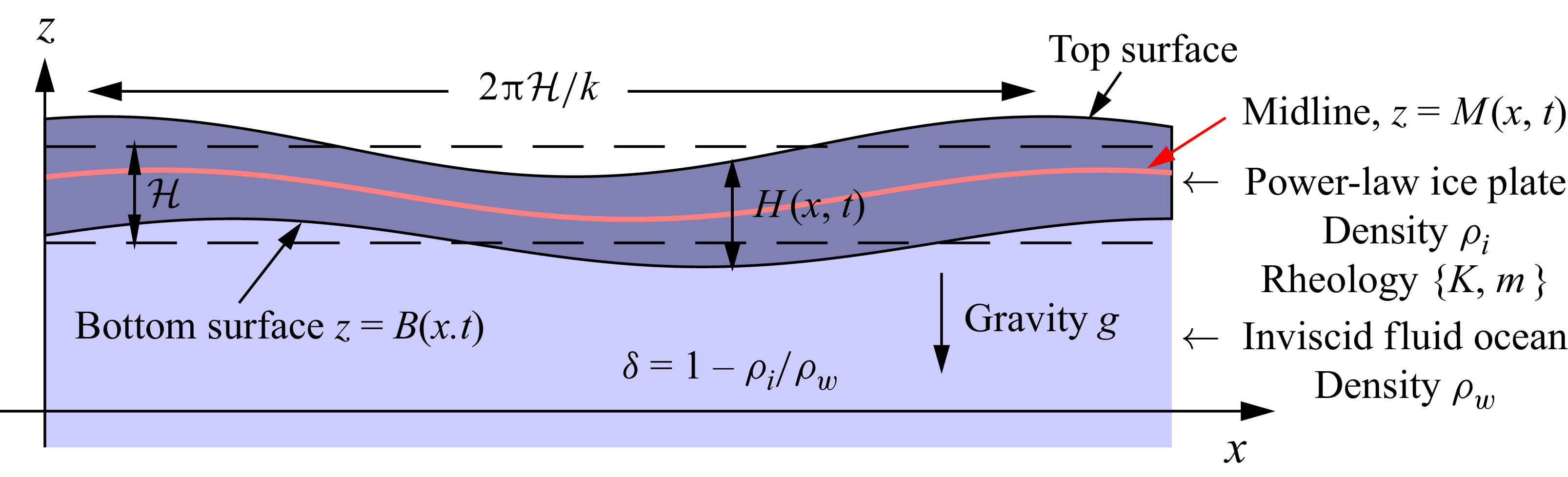


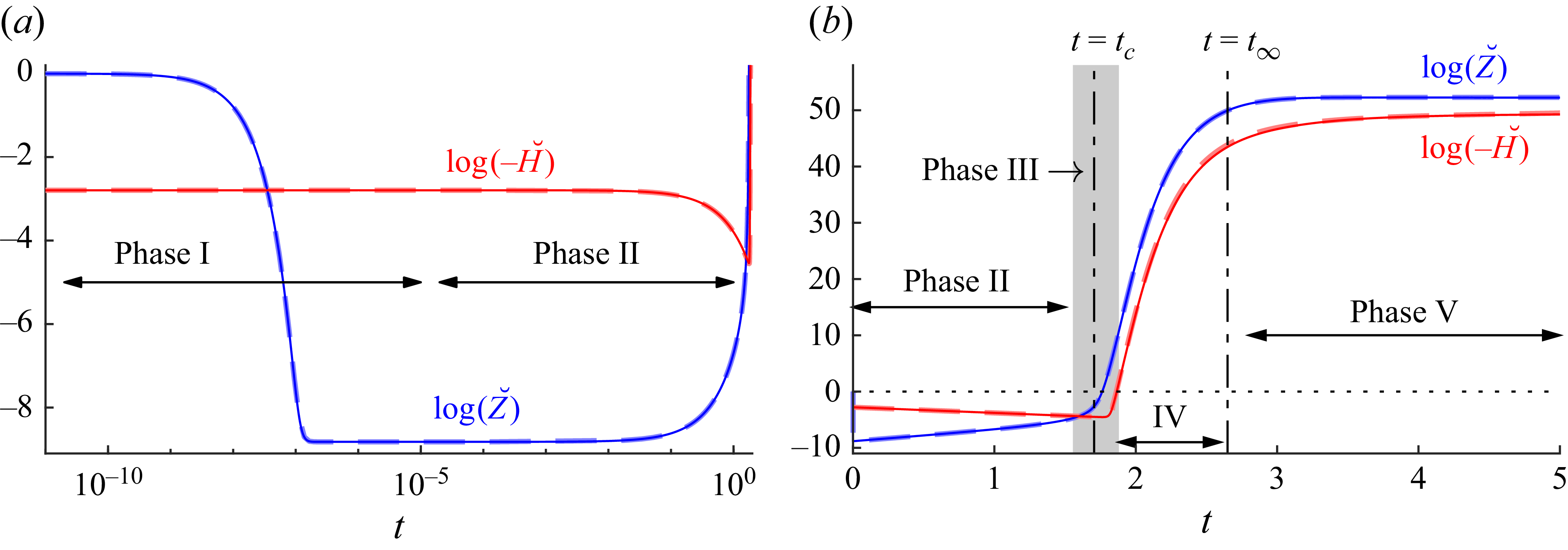


 Open access