





1. Introduction
Instabilities at liquid–liquid interfaces play an important role in many familiar phenomena, from the break up of a water column leaving a faucet (Plateau Reference Plateau1873; Rayleigh Reference Rayleigh1879) to the formation of trains of soap bubbles (Eggers & Villermaux Reference Eggers and Villermaux2008) and the dendritic morphology of snowflakes (Langer Reference Langer1980). Small scale fluid flow confined by solid boundaries is fundamental to many such situations. On these scales, surface forces dominate over body forces and thus capillarity plays a dominant role in controlling the flow. Capillary flows arise from the deformation of an interface, so the shape of the confinement is critical to the behaviour of such instabilities. Take, for example, the Saffman–Taylor (or ‘viscous fingering’) instability (Saffman & Taylor Reference Saffman and Taylor1958), which classically occurs when a liquid of lower viscosity displaces a liquid of higher viscosity in a channel whose width is uniform; this instability can be suppressed by either varying the channel width in space (Al-Housseiny, Tsai & Stone Reference Al-Housseiny, Tsai and Stone2012; Al-Housseiny & Stone Reference Al-Housseiny and Stone2013; Reyssat Reference Reyssat2014) or in time (Zheng, Kim & Stone Reference Zheng, Kim and Stone2015). (Indeed, channel tapering can even promote an ‘opposite’ instability in which less viscous liquid is able to displace more viscous liquid from the apex of a wedge Keiser et al. Reference Keiser, Herbaut, Bico and Reyssat2016.) On scales that are smaller still, there is evidence that evaporation driven instabilities common in drying of microelectromechanical systems have a sensitive dependence on the geometry of the channel (Hadjittofis et al. Reference Hadjittofis, Lister, Singh and Vella2016; Ledesma-Aguilar et al. Reference Ledesma-Aguilar, Laghezza, Yeomans and Vella2017; Ha et al. Reference Ha, Kim, Siu and Tawfick2021, for example).
In each of the above examples, a rigid geometry is imposed externally upon the liquid. However, new possibilities open up if the walls confining the liquid are flexible; in this case, the presence of liquid can feed back on the channel geometry, with the potential to significantly affect the behaviour of the instability. A hint of this can be found in the experiments of Seemann et al. (Reference Seemann2011), snapshots of which are shown in figure 1(a). In these experiments, a humid environment results in droplets condensing into an array of deformable microchannels which is described by Seemann et al. (Reference Seemann2011) as elastic. As condensation proceeds, the surface of the droplets moves towards the free end of the channels (the ends closest to the camera in figure 1b, which corresponds to out of the page in figure 1a), and the droplets spontaneously arrange into a periodic pattern. It is natural to suspect that the periodic pattern is the result of the growth of an interfacial instability that relies on fluid-induced deformations of the channel walls. In more detail: in these experiments, droplets of liquid condense into a three-dimensional array of channels (shown schematically in figure 1b); the Laplace pressure within the droplets is positive because the channel walls are non-wetting, resulting in an outward deformation of the adjacent channel walls, which grows further as the volume of liquid continues to grow via condensation. Increases in channel wall deformation tend to promote the pattern formation (the presence of liquid only in isolated regions) by reducing the meniscus pressure at the widest points (the pressure is inversely proportional to channel width) thus promoting liquid flow towards those points and encouraging localization into droplets (figure 1b). By contrast, if the channel walls were rigid and parallel, the meniscus pressure would be uniform and there would, therefore, be no preference for localization.
(a) Snapshots of experiments performed by R. Seemann (personal communication), similar to those published by Seemann et al. (Reference Seemann2011), in which liquid droplets are condensed within an array of deformable microchannels. The interaction between the droplets and deformable boundaries leads to a pattern of drops in neighbouring channels offset relative to one another, and with a characteristic droplet spacing and size. (b) Schematic diagram of the experiments shown in panel (a). Here, droplets are shaded blue, flexible channel walls are shaded grey and the base of the array is shaded red. It is not clear in the experiments whether the droplets extend to the base of the channels or not (personal communication). Black dashed lines indicate where the top of the channel walls would be located, if they were undeformed. We refer to variations in the direction parallel to the channel walls as ‘in-plane’ and those perpendicular to that direction as ‘transverse’, as indicated.

The complex contact line, as well as possible interaction between droplets in neighbouring channels, adds significant complexity to a conceptual description of the instability that results in the periodic pattern of figure 1(a). In this paper, we consider a simplified setup, shown schematically in figure 2, in which the channel is rotated relative to figure 1(b) so that its ‘base’ is on the left: a single channel consisting of two flexible walls and a rigid base, which is part filled with liquid. This set-up retains the interaction between capillary flow and bending deformations (or ‘bendocapillarity’), and hence captures the essence of the instability, whilst removing the complexity of the contact line geometry and interaction between droplets in neighbouring channels. We also consider only a constant droplet volume, simplifying the system considerably (this assumption is reasonable because condensation occurs very ‘slowly’ in the experiments, though we can only quantify this statement in due course). We stress that we are not attempting to entirely describe the mechanism responsible for the instability shown in figure 1, rather we seek to understand the fundamental aspects of instabilities resulting from channel wall deformations in two dimensions under capillary forces.
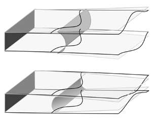
Schematic representation of the air–liquid interface in the bendocapillary instability for (a) non-wetting and (b) wetting liquids. In each case, the grey and black outlines indicate the configuration (channel shape and contact line) prior and post perturbation, respectively. Upon perturbing, the contact line is deformed from a straight line to a periodic curve; in both wetting and non-wetting cases, the channel experiences a deformation that enhances (reduces, respectively) the deformation of the channel walls in the base state in regions adjacent to protrusions (invaginations). Note that the configurations shown in this figure are oriented in a way that is rotated  $90^{\circ }$ relative to the configuration shown in figure 1(b).
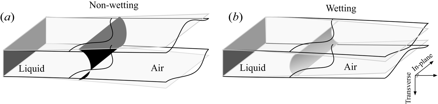
The mechanism for instability in this set-up is elucidated in figure 2. The base state has a stationary interface, which is uniform in the in-plane direction. For a non-wetting liquid with a positive Laplace pressure, the channel walls are tapered outwards (figure 2a). At protrusions of a perturbation to this interface, there will be a reduced confinement from the channel walls, which results from the combination of two complementary effects: (1) the interface advancing further into the channel, whose walls are tapered outwards in this direction; and (2) the elastic response of the channel walls to the advance of the interface, which takes the form of an enhanced outwards deformation (the positive Laplace pressure is now applied over a longer length). This reduction in confinement tends to reduce the liquid pressure at these protrusions (the pressure is inversely proportional to the channel width); the perturbation will grow, and the instability will be amplified, if the total pressure reduction from the combination of these two effects exceeds the (stabilizing) pressure increase that results from an interface that is now locally convex in the in-plane direction, i.e. if the wavelength of the perturbation is sufficiently long.
Perhaps surprisingly, a similar mechanism is also applicable to wetting configurations. In the wetting case, the bulk liquid pressure is negative and the associated channel deformations are inwards, but the result is the same: protrusions now advance into a narrower channel, which is further enhanced by the additional elastic response. The combination of these two effects reduces the local liquid pressure (it becomes more negative), which can, again, cause the perturbation to grow if its wavelength is sufficiently long. Therefore, both wetting and non-wetting liquids may experience this bendocapillary instability in the same channel. This is in contrast to the similar systems described by Al-Housseiny et al. (Reference Al-Housseiny, Tsai and Stone2012) and Keiser et al. (Reference Keiser, Herbaut, Bico and Reyssat2016) featuring rigid, tapered channel walls.
In this paper, we investigate this instability mechanism quantitatively. We begin by presenting a simple scaling argument for the wavenumber of unstable modes and the associated growth rates, before developing a formal mathematical model of the system shown in figure 2. The model equations are then non-dimensionalized; in doing so, we identify three key dimensionless parameters that characterize the aspect ratio of the channel, the ability of the liquid to deform it and the amount of liquid it contains. Following this, in § 4, we set out the base states (equilibria) of the system, which are parametrized by these three dimensionless numbers; these equilibria are essentially those described by Taroni & Vella (Reference Taroni and Vella2012), but we extend this description to include non-wetting configurations. In § 5, we consider the linear stability of these equilibria. We numerically solve the equations that must be satisfied by perturbations and identify several important, yet generic, features of these solutions. In particular, equilibria are linearly unstable to perturbations of sufficiently small wavenumber (large wavelength), with maximum growth rates that increase with both the channel bendability and amount of liquid in the channel. In § 6, we consider the limiting case of small channel deformations. Using asymptotic methods, we examine the system of equations that perturbations must satisfy in this limit, deriving a universal dispersion relation and verifying analytically the observations of § 5. Finally, in § 7, we discuss and summarize the results and provide concluding remarks.
2. Scaling argument for the basic mechanism
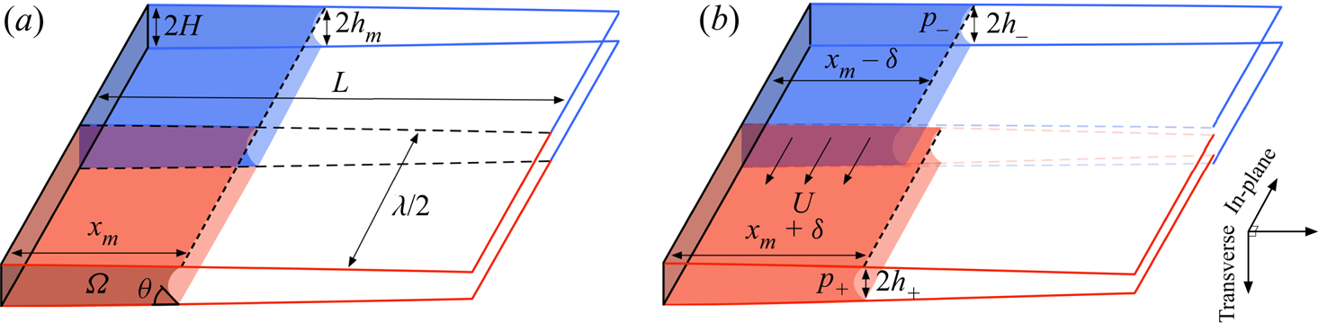
Before developing a detailed mathematical model, we seek first to gain quantitative insight into the mode selection that results from the mechanism described in § 1. We consider the configuration shown in figure 3: a section of a channel of width  $\lambda$ and length $L$ contains liquid that sits adjacent to a rigid base of thickness $2H$. The walls are clamped at the rigid base, while the opposite end is open. These side walls are narrow and flexible; they bend in response to the liquid pressure and are characterized by a bending stiffness $B$. For the purposes of this scaling argument, we imagine a cut along their centre (black dashed lines in figure 3a), allowing either side of this cut to deform independently of the other. We restrict deformations to the transverse direction, so that each half is itself uniform in the in-plane direction. (Note that the schematic shown in figure 3 corresponds to a wetting configuration, but the scaling argument set out in this section is also applicable for non-wetting configurations.)
Schematic diagrams of a section of a flexible channel consisting of a solid base and two flexible walls, which are only permitted to bend in the transverse direction. A cut along the centre of the channel (black dashed line) allows the two halves to bend independently of one another. (a) The system is in equilibrium with the meniscus located a distance  $x_m$ from the base (the left-hand end, in this orientation). (b) The equilibrium is perturbed by moving the menisci on either side of the cut a distance $\delta$; as described in the main text, if $\lambda$ is sufficiently large, this perturbation results in the flow of liquid from troughs (blue) to peaks (red) with speed $U > 0$, amplifying the perturbation. Note that the configurations shown in this figure are oriented in a direction rotated $90^{\circ }$ relative to the configuration shown in figure 1(b).
2.1. Base state
Taroni & Vella (Reference Taroni and Vella2012) considered the two-dimensional analogue of this system, in which both halves are identical, and showed that equilibrium configurations always exist when the cross-sectional volume of liquid  $\varOmega$ is sufficiently small. In particular, this means that equilibria always exist when $\varOmega / (2HL) \ll 1$ and the cross-sectional volume of liquid is small in comparison with the cross-sectional channel volume. Here we consider such an equilibrium with a meniscus that is located a distance denoted $x_m$ from the clamped end (figure 3). The restriction to relatively small volumes means that the channel walls are not deformed significantly and thus $h_m$ – the half-width at the meniscus – scales with the clamped end width, i.e. $h_m \sim H$. By conservation of mass, the meniscus position $x_m \sim \varOmega / H$ and the liquid pressure $p_m \sim -\gamma \cos \theta /H$, where $\gamma$ is the surface tension coefficient of the liquid and $\theta$ is the constant contact angle between the liquid and channel wall.
Before we consider perturbations to this equilibrium, we require a scaling for  $h_m'$, the channel slope. By considering a cantilever beam with bending stiffness $B$ deformed over a length scale $x_m$ by a uniform (Laplace) pressure $-\gamma \cos \theta / H$, we find (Timoshenko & Woinowsky-Krieger Reference Timoshenko and Woinowsky-Krieger1959)
 \begin{equation} h_m' \sim{-}\frac{\gamma \cos \theta x_m^3}{B H}. \end{equation}
2.2. Mode selection
We mimic a periodic perturbation of wavenumber  $k = 2{\rm \pi} /\lambda$ and amplitude $\delta$ by considering a region of length $\lambda$ in the in-plane direction, centred around the cut (figure 3). We imagine forcing one side of the cut to advance uniformly to $x_0 + \delta$ and the other to retreat to $x_0 - \delta$ (figure 3b). As discussed, the transverse interfacial curvature, and thus liquid pressure, changes as a result of this perturbation: in this wetting example, the protruding half of the interface is forced into a stronger confinement by the tapering of the equilibrium configuration, and this confinement is enhanced by the elastic response of the channel to the change in meniscus position. Note that in this idealized scenario, the interface consists of two discrete halves, each of which is uniform in the in-plane direction, and therefore does not naturally include the stabilizing effect of in-plane curvature variations. To account for this stabilizing curvature in the context of the square wave perturbation, we add a pressure penalty of $\gamma \delta k^2$ to the protruding half (the $k^2$ term is introduced to represent the second derivative of a perturbation acting over a wavelength $1/k$, i.e. smoothing out the square wave perturbation to be effectively sinusoidal).
The perturbation will grow provided that the difference in liquid pressure between the two halves,  $\Delta P = p_+ - p_-$, drives liquid towards the protruding half (the red half in figure 3b), i.e. when $\Delta P<0$.
To leading order in  $\delta$, we find that
 \begin{equation} \Delta P\sim \gamma\left(\frac{\cos \theta}{h_-} - \frac{\cos \theta}{h_+} + \beta \delta k^2\right) \sim \gamma \left(\frac{\Delta h \cos \theta}{h_m^2} + \beta \delta k^2\right), \end{equation}
where  $\beta >0$ is an ${O}(1)$ scaling constant and $\Delta h = h_+ - h_-$ is the difference in the channel widths at the menisci between the two halves (see figure 3b). For wetting configurations, with $\cos \theta > 0$, we expect $\Delta h < 0$, while for non-wetting configurations with $\cos \theta < 0$, we expect that $\Delta h > 0$; the first term in (2.2), which represents the transverse contribution to curvature changes, is therefore negative regardless of the wettability and thus promotes instability.
To find a scaling for  $\Delta h$, we decompose it into a contribution from the meniscus advancing into a tapered channel and a contribution from the elastic response to the perturbation:
 \begin{equation} \Delta h = \Delta h_{tapering} + \Delta h_{elastic}. \end{equation}
 To leading order in  $\delta$, the tapering contribution has the same scaling as a meniscus advancing into a rigid channel whose angle is set by the equilibrium configuration, i.e.
 \begin{equation} \Delta h_{tapering} \sim \delta \times h_m' \sim{-}\delta \frac{\gamma \cos \theta x_m^3}{B H}, \end{equation}
where we have used the scaling (2.1) for  $h_m'$.
The leading order elastic contribution is found by considering a cantilever beam of length  $x_m$ that is loaded with the equilibrium liquid pressure $p_m = -\gamma \cos \theta /H$ (the dry region of the beam offers no resistance to bending in this scenario (Bradley et al. Reference Bradley, Box, Hewitt and Vella2019)). If the length of this cantilever beam is then increased to $x_m + \delta$, the corresponding increase in deflection of its tip is
 \begin{equation} \Delta h_{elastic} \sim{-}\frac{p_m}{B}[\left(x_m + \delta\right)^4 - x_m^4]. \end{equation}
By expanding the right-hand side of (2.5), retaining only leading order terms in  $\delta$, and inserting the meniscus pressure scaling $p_m \sim -\gamma \cos \theta / H$, we obtain the scaling
 \begin{equation} \Delta h_{elastic}\sim{-}\delta \frac{\gamma \cos \theta x_m^3}{BH}. \end{equation}
 Perhaps surprisingly, both the elastic (2.6) and tapering (2.4) contributions to  $\Delta h$ (2.3) have the same scaling. Substituting these scalings into (2.2)–(2.3) gives
 \begin{equation} \Delta P \sim{-}\delta \gamma \left(\frac{\gamma \cos^2 \theta}{H^2}\frac{ x_m^3}{B H} - \beta k^2\right). \end{equation}
By balancing the terms in (2.7), we obtain a scaling for a critical wavenumber:
 \begin{equation} k_c \sim \left(\frac{\gamma \cos^2 \theta x_m^3}{B H^3}\right)^{1/2}. \end{equation}
We expect that perturbations with wavenumber  $k \lesssim k_c$ will be unstable, while those with wavenumber $k \gtrsim k_c$ will be damped.
2.3. Growth rates
When  $\Delta P < 0$, liquid is sucked from the invaginations into protrusions with a typical velocity $U$ (figure 3b), whose scaling we now consider. To estimate this velocity scale, we note that this pressure difference acts over a length scale $\lambda = 2{\rm \pi} /k$ and so lubrication theory (Leal Reference Leal2007) suggests that (provided $\lambda,L \gg H$)
 \begin{equation} U \sim{-}\frac{H^2}{\mu}\frac{\Delta P}{\lambda}\sim \frac{H^2}{\mu} \delta \gamma k\left(\frac{\gamma \cos^2 \theta}{H^2}\frac{x_m^3}{B H} - \beta k^2\right), \end{equation}
where  $\mu$ is the viscosity of the liquid. The corresponding flux of liquid between the two halves of the channel is
 \begin{equation} Q \sim \varOmega U \sim\frac{H^2}{\mu} \delta \gamma k \varOmega\left(\frac{\gamma \cos^2 \theta}{H^2}\frac{x_m^3}{B H} - \beta k^2\right), \end{equation}
while conservation of mass for either section requires
 \begin{equation} H \lambda \frac{\mathrm{d} \delta}{\mathrm{d} t} \sim Q. \end{equation}
Combining (2.10) and (2.11) gives a scaling for  $\sigma$, the growth rate of perturbations, as
 \begin{equation} \sigma = \frac{1}{\delta} \frac{\mathrm{d} \delta}{\mathrm{d} t} \sim \frac{\varOmega H \gamma}{\mu}\left(\frac{\gamma \cos^2 \theta}{H^2} \frac{x_m^3}{B H} - \beta k^2\right)k^2. \end{equation}
 The wavenumber of the fastest growing modes is determined by a balance of the bracketed terms in (2.12) and can be seen to yield  $k \sim k_c$, with $k_c$ as given in (2.8). The corresponding growth rate of perturbations with wavenumbers of this characteristic size scales as
 \begin{equation} \sigma_c = \frac{1}{\delta} \frac{\mathrm{d} \delta}{\mathrm{d} t} \sim \frac{\gamma^{3} \cos^{4} \theta x_m^7}{\mu B^{2} H^{4}}, \end{equation}
where we have made use of the small deformation volume scaling,  $\varOmega \sim x_m H$.
The dispersion relation (2.12) can be expressed as  $\sigma \sim (k_*^2-k^2)k^2$ for some $k_*$. This form of the dispersion relation as a function of $k$ is reminiscent of that for the Rayleigh–Plateau instability, which describes the surface-tension driven breakup of a liquid jet falling under its own weight (Plateau Reference Plateau1873; Rayleigh Reference Rayleigh1879, Reference Rayleigh1892). However, the important distinction between the dispersion relation (2.12) and that arising in the Rayleigh–Plateau analysis is that the $-k^4$ in (2.12) is a result of bending stiffness, rather than surface tension, from which the $-k^4$ arises in the Rayleigh–Plateau analysis.
While the above calculations are rough, they suggest that both wetting and non-wetting configurations of sufficiently small wavenumber will be amplified, and that both the fastest growing mode and corresponding growth rate are symmetric under a reversal of wettability ( $\cos \theta \to -\cos \theta$). Moreover, the growth rate of unstable modes has an extremely sensitive dependence on the amount of liquid in the channel (via the meniscus position $x_m$). We now turn to a more formal calculation to interrogate these observations in detail, but shall refer back to the results of this section in due course, since this argument distils our main results.
3. Mathematical model
In this section, we develop a formal mathematical model of the system discussed in § 2. The configuration is shown in figure 4(a): a narrow cell of thickness  $2H$ and length $L$ extends infinitely in the $y$-direction. The channel has a rigid boundary at $x = 0$ and is free at $x = L$. The other two walls are flexible and, when undeformed, coincide with the planes $z = \pm H$. These channel walls are characterized by their thickness $b$, Young's modulus $E$ and Poisson's ratio $\nu$. We shall assume that channel walls are relatively thin ( $b \ll L$) and may therefore be characterized by their bending stiffness $B = Eb^3 / [12(1-\nu ^2)]$. We shall take $\nu = 0.5$, corresponding to incompressible walls, throughout.
(a) Schematic diagram of liquid in a channel consisting of a solid, impenetrable base at  $x =0$ and two flexible walls, whose mid-planes are located at $z = \pm h(x,y,t)$. The liquid (a wetting liquid in this case) makes contact with the channel walls at the contact line $x = x_m(y,t)$. The cell extends infinitely in the $y$-direction, only a section of which is shown. (The channel is assumed narrow, $H / L \ll 1$, but here we exaggerate $H/L$ for clarity.) (b) Cross-sections of the system shown in panel (a) through the $(x,y)$ plane (upper) and $(x,z)$ plane (lower); the latter is taken through $y = y^*$, indicated by the dashed box in panel (a).

Liquid of viscosity  $\mu$ and surface tension $\gamma$ sits at the solid base of the channel. We assume that the liquid makes a constant contact angle $\theta$ with the channel walls (i.e. any dynamic contact angle effects are ignored). The liquid pressure induces a deformation of the channel walls; in the following sections, we describe the coupled models for the flow of liquid and deformation of the channel walls, and then non-dimensionalize the resulting system of equations.
3.1. Preliminaries and assumptions
We assume that the configuration is symmetric about  $z = 0$, and therefore only need to consider a single channel wall. Alongside our assumption that the flexible channel walls are thin in comparison with their length, this symmetry assumption means that we can characterize the channel width at time $t > 0$ entirely by the position of the mid-plane of one wall (Reddy Reference Reddy2006), which is denoted by $h(x,y,t)$.
The channel is wetted over the region  $0 < x < x_m(y,t)$. We assume that $x_m \gg H$ throughout, and also that variations in the flow in the $y$-direction occur on a length scale much longer than $H$, allowing us to use lubrication theory to model the liquid flow. Since the channel geometry does not provide a natural length scale for flow in the $y$-direction, we postpone discussion of the $y$-length scale until § 3.4 and verify this latter assumption a posteriori. With these assumptions, the contact angle between liquid and solid is approximately that measured in the $(x,z)$ plane (figure 4b, bottom panel).
Finally, we neglect the weight and inertia of both the liquid and the channel walls, as well as the line force associated with surface tension, which have been shown to be unimportant in comparison with the Laplace pressure of the liquid in similar situations (Taroni & Vella Reference Taroni and Vella2012; Bradley et al. Reference Bradley, Box, Hewitt and Vella2019; Bradley Reference Bradley2020).
3.2. Liquid flow
The fluid flow is described using lubrication theory. The evolution of the pressure field  $p(x,y,t)$ and the channel width $2h(x,y,t)$ are then coupled via Reynolds’ equation
 \begin{equation} \frac{\partial h}{\partial t} = \boldsymbol{\nabla} \boldsymbol{\cdot} \left(\frac{h^3}{3\mu} \boldsymbol{\nabla} p\right)\quad \text{in}\ 0 < x < x_m(y,t). \end{equation}
The free boundary of the liquid moves in response to the flux of fluid there. Ignoring any condensation or evaporation, the flux of fluid through the menisci must balance that caused by motion and thus the following kinematic condition must hold:
 \begin{equation} \frac{\partial x_m}{\partial t} ={-}\left.\frac{h^2}{3\mu}\boldsymbol{\nabla} p \boldsymbol{\cdot} \frac{\boldsymbol{n}}{|\boldsymbol{n}|}\right|_{x = x_m(y,t)}. \end{equation}
Here,  $\boldsymbol {n} = \boldsymbol {e}_x -\partial _y x_m \boldsymbol {e}_y$ is the normal to the interface in the $(x,y)$ plane (figure 4b).
According to Laplace's law, the liquid pressure adjacent to the interface is
 \begin{equation} p(x = x_m, y,t) = \gamma(C_{{\perp}} + C_{{\parallel}}), \end{equation}
where  $C_{\perp }$ and $C_{\parallel }$ are the transverse and in-plane interfacial curvatures, respectively. Our neglect of gravity means that the meniscus is a minimal surface: in the $(x,z)$ plane, the menisci are therefore approximately arcs of circles (figure 4b) with curvatures
 \begin{equation} C_{{\perp}} ={-}\frac{\cos \theta}{h(x=x_m,y,t)}. \end{equation}
Our assumption that variations in the  $y$-direction occur on a length scale much larger than $H$ means that we can approximate the in-plane interfacial curvature by
 \begin{equation} C_{{\parallel}} ={-}\frac{\partial ^2 x_m}{\partial y^2}. \end{equation}
Finally, we impose a no-flux condition at the impenetrable base:
 \begin{equation} \frac{\partial p}{\partial x}=0 \quad \text{at}\ x =0. \end{equation}
3.3. Wall deformation
The channel walls are modelled as thin plates and the position of their mid-planes is  $z = \pm (h(x,y,t) + b/2)$, where $b$ is the wall thickness. The bending of the walls in response to the fluid pressure requires the following to hold
 \begin{equation} B\nabla^4 h = p, \end{equation}
where  $p$ is the liquid pressure in $0 < x < x_m(y,t)$ and zero in $x_m(y,t) < x < L$.
In fact, the wall deformation results from both bending and stretching of the thin plates, and can be modelled more generally by the Föppl–von Kármán equations (von Kármán Reference von Kármán1910; Föppl Reference Föppl1921), which include additional second derivatives of  $h$ multiplying the in-plane tension in the plates. There are two possible sources of this tension: first, the ‘base-state’ tension that arises even in the case of a uniform ( $y$-independent) deflection, which is caused by the tangential component of the capillary force acting across the contact line, and second, the tension induced by the deformation of the wall itself. Both of these can be considered negligible for the following reasons. First, since the free ends of the walls are stress free, any base-state tension is introduced only over the length of the wetted portion of the walls, which scales with $L$. The size of this tension scales with the surface tension $\gamma$; the resulting terms in (3.7) are negligible compared to the pressure term (of order $\gamma /h$) provided $h/L \ll 1$, which we have already assumed in our application of lubrication theory. Second, the base-state deflection of the walls (referred to later as $h_e(x)$) is $y$-invariant and thus involves only bending, not stretching, and therefore does not itself induce any tension in the walls. However, $x$- and $y$-dependent perturbations to this base state do induce non-zero curvature in two dimensions, and necessarily require stretching. This stretching is proportional to the square of the additional deflection $\tilde {h}$ and the induced tension is of order $Eb(\tilde {h}/L)^2$. Since we are only interested in small perturbations (indeed, we only study the linear stability problem in which the perturbations $\tilde {h}$ are formally infinitesimal), the resulting contributions to (3.7) will also be negligible. We anticipate that for larger spatially variable deflections of the walls (such as those that perhaps occur in the experiments in figure 1), the deformation-induced tension may indeed become significant and the wall deflections would need to be modelled with the full Föppl–von Kármán equations. However, for the purposes of this study, we restrict ourselves to the simpler approximation (3.7).
To close the problem, we require boundary conditions at the channel ends,  $x= 0$ and $x = L$, as well as at the interface, $x = x_m$. We apply a straightforward clamped condition at $x = 0$,
 \begin{equation} h= H,\quad \frac{\partial h}{\partial x} = 0,\quad \text{at}\ x = 0. \end{equation}
 The channel walls are free at  $x = L$; for a thin plate undergoing pure bending deformations, free boundary conditions are imposed by requiring (Timoshenko & Woinowsky-Krieger Reference Timoshenko and Woinowsky-Krieger1959)
 \begin{equation} \frac{\partial ^2 h}{\partial x^2} + \nu \frac{\partial ^2 h}{\partial y^2} =0,\quad \frac{\partial ^3 h}{\partial x^3} + (2-\nu) \frac{\partial ^3 h}{\partial x \partial y^2} = 0,\quad \text{at}\ x = L. \end{equation}
The boundary condition (3.9a,b) applies only when the channel walls do not touch. If the channel walls touch – as might ultimately occur in the wetting case, where the walls are drawn towards one another – the boundary condition (3.9a,b) must be modified to include a repulsive shear force. This touching ends scenario requires significant deformations, which are not consistent with the relatively small volumes that are of primary interest here; we therefore assume that (3.9a,b) holds throughout.
At the meniscus, we assume that the channel and its slope, as well as the moments and shear forces it supports, are continuous:
 $$\begin{gather} \left[h \right]_{-}^{+} = 0 \quad \text{[continuous channel shape]}, \end{gather}$$
 $$\begin{gather}\left[\frac{\partial h}{\partial x} \right]_{-}^{+} = \left[\frac{\partial h}{\partial y} \right]_{-}^{+} =0 \quad \text{[continuous channel slope],} \end{gather}$$
 $$\begin{gather}\left[\frac{\partial ^2 h}{\partial x^2} + \nu \frac{\partial ^2 h}{\partial y^2} \right]_{-}^{+} = \left[\frac{\partial ^2 h}{\partial y^2} + \nu \frac{\partial ^2 h}{\partial x^2} \right]_{-}^{+} = \left[\frac{\partial ^2 h}{\partial x \partial y} \right]_{-}^{+} = 0 \quad \text{[continuous bending moments],} \end{gather}$$
 $$\begin{gather}\left[\frac{\partial ^3 h}{\partial x^3} + \frac{\partial ^3 h}{\partial x\partial y^2}\right]_{-}^{+} = \left[\frac{\partial ^3 h}{\partial x^2 \partial y} + \frac{\partial ^3 h}{\partial y^3} \right]_{-}^{+} =0 \quad \text{[continuous shear forces].} \end{gather}$$
Here,  $[ f ]_-^+ = f(x_m^+,y,t) - f(x_m^-,y,t)$ denotes the jump in the quantity $f$ across $x = x_m$, and has both $y$- and $t$-dependence in general.
In summary, the system is described by the liquid pressure  $p$ and wall deflection $h$, which satisfy the coupled partial differential equations (PDEs) (3.1) and (3.7) for the fluid flow and wall deformation, respectively. This system of PDEs is to be solved alongside the kinematic condition (3.2), the no-flux condition (3.6), the clamped end condition (3.8a,b), the free end condition (3.9a,b) and the continuity conditions (3.10)–(3.13). We now turn to a non-dimensionalization of this system.
3.4. Non-dimensionalization
The system of model equations is non-dimensionalized by scaling variables appropriately. Variations in the  $x$- and $z$-directions have natural length scales set by the channel geometry, and corresponding dimensionless variables (denoted by hats)
 \begin{equation} \hat{h} = \frac{h}{H},\quad \hat{x} = \frac{x}{L},\quad \hat{x}_m = \frac{x_m}{L}. \end{equation}
 The channel geometry does not provide a length scale for variations in the  $y$-direction, so we choose the scale $L$ used in the $x$-direction, introducing
 \begin{equation} \hat{y} = \frac{y}{L}. \end{equation}
Note that in the scaling argument of § 2, we identified a critical wavelength for instability in the  $y$-direction,
 \begin{equation} L_y = \left(\frac{B H^3}{\gamma \cos^2 \theta L^3}\right)^{1/2}, \end{equation}
and so we anticipate the appearance of the dimensionless wavenumber
 \begin{equation} L/L_y = \left(\frac{\gamma \cos^2 \theta L^5}{B H^3}\right)^{1/2} \end{equation}
in our stability analysis.
Time and pressure variables are non-dimensionalized by scaling with a capillary time scale and a bending pressure scale, respectively,
 \begin{equation} \hat{t} =\frac{t}{\tau_c} = \frac{|\gamma \cos \theta| H}{\mu L^2}t,\quad \hat{p} = \frac{L^4}{B}p. \end{equation}
Using values from Bradley et al. (Reference Bradley, Box, Hewitt and Vella2019), who studied a similar bendocapillary system, the typical capillary timescale  $\tau _c$ is of the order of 10 s; this is significantly shorter than the timescale on which the channels in the motivating experiments (figure 1a) fill via condensation, which is of the order of minutes. The constant-volume model considered here is therefore appropriate for these experiments.
After applying the scalings above, the PDE system (3.1) and (3.7) becomes
 \begin{align} \frac{\partial \hat{h}}{\partial \hat{t}} &=\frac{1}{3|\varGamma|}\hat{\boldsymbol{\nabla}}\boldsymbol{\cdot} [\hat{h}^3\hat{\boldsymbol{\nabla}}\hat{p}] \quad \quad \quad \quad 0 < \hat{x} < \hat{x}_m(\hat{y},\hat{t}), \end{align}
 \begin{align}\hat{p}&=0 \quad \quad \quad \quad \hat{x}_m(\hat{y},\hat{t}) < \hat{x} < 1, \end{align}
 \begin{align}\hat{p} &=\hat{\nabla}^4 \hat{h} \quad \quad \quad \quad 0 < \hat{x} < 1. \end{align}
Here,
 \begin{equation} \varGamma = \frac{\gamma \cos \theta L^4}{B H^2} \end{equation}
is the channel ‘bendability’ and characterizes the ability of the typical capillary pressure within the liquid to bend the channel walls: large  $|\varGamma |$ indicates that the channel walls are easily deformed (achieved by having low bending stiffness or high surface tension, for example), and vice versa for small $|\varGamma |$. The sign of $\varGamma$ captures the wetting conditions: $\varGamma > 0$ corresponds to wetting conditions ( $\cos \theta >0$), while $\varGamma < 0$ corresponds to non-wetting conditions ( $\cos \theta <0$).
Note that the sixth-order PDE that results from combining (3.19)–(3.21) is a two-spatial-dimension analogue to PDEs that often appear in studies of fluid structure interactions at low Reynolds number (see Flitton & King (Reference Flitton and King2004), Aristoff, Duprat & Stone (Reference Aristoff, Duprat and Stone2011), Duprat, Aristoff & Stone (Reference Duprat, Aristoff and Stone2011), for example).
After non-dimensionalizing, the boundary conditions (3.8a,b)–(3.9a,b) and (3.10)–(3.13) on the channel wall position become
 $$\begin{gather} \hat{h} = 1,\quad \frac{\partial \hat{h}}{\partial \hat{x}} = 0 \quad \text{at}\ \hat{x} = 0, \end{gather}$$
 $$\begin{gather}\frac{\partial ^2 \hat{h}}{\partial \hat{x}^2} + \nu \frac{\partial ^2 \hat{h}}{\partial \hat{y}^2} = 0, \quad \frac{\partial ^3 \hat{h}}{\partial \hat{x} ^3} + (2-\nu) \frac{\partial ^3 \hat{h}}{\partial \hat{x}\partial y^2}=0 \quad \text{at}\ \hat{x} = 1, \end{gather}$$
 $$\begin{gather}\left[ \hat{h} \right]_{-}^{+} = \left[\frac{\partial \hat{h}}{\partial \hat{x}}\right] _{-}^{+} = \left[\frac{\partial \hat{h}}{\partial \hat{y}} \right]_{-}^{+} = 0, \end{gather}$$
 $$\begin{gather}\left[\frac{\partial ^2 \hat{h}}{\partial \hat{x}^2} +\nu \frac{\partial ^2 \hat{h}}{\partial \hat{y}^2} \right]_{-}^{+} = \left[\frac{\partial ^2 \hat{h}}{\partial \hat{y}^2} +\nu \frac{\partial ^2 \hat{h}}{\partial \hat{x}^2} \right]_{-}^{+} = \left[\frac{\partial ^2 \hat{h}}{\partial \hat{x} \partial \hat{y}} \right]_{-}^{+} = 0, \end{gather}$$
 $$\begin{gather}\left[\left(\frac{\partial ^3 \hat{h}}{\partial \hat{x}^3} + \frac{\partial ^2 \hat{h}}{\partial \hat{x} \partial \hat{y} ^2}\right) \right]_{-}^{+} = \left[ \left(\frac{\partial ^2 \hat{h}}{\partial \hat{x}^2 \partial y} + \frac{\partial ^2 \hat{h}}{\partial \hat{y} ^3}\right) \right]_{-}^{+} =0 , \end{gather}$$
where the jump conditions in (3.25)–(3.27) are now (and henceforth) evaluated across the dimensionless meniscus position  $\hat {x}_m(y,t)$.
The boundary conditions (3.3) and (3.6) on the pressure become
 \begin{equation} \frac{\partial \hat{p}}{\partial \hat{x}} = 0 \quad \text{at}\ \hat{x} = 0,\quad \hat{p} ={-}\varGamma\left(\frac{1}{\hat{h}} + a \frac{\partial ^2 \hat{x}_m}{\partial \hat{y}^2}\right)\quad \text{at}\ \hat{x} = \hat{x}_m. \end{equation}
Here,  $a = H/(L \cos \theta )$ is a reduced channel aspect ratio, which arises as the ratio between the typical radii of curvature in the transverse and in-plane directions. Note that $a$ always has the same sign as $\varGamma$. In particular, this means that their ratio $\varGamma / a$, which shall appear frequently, is always positive.
We retain the final term in (3.28a,b) despite it being higher order in  $a \ll 1$ (we assume $\cos \theta \sim {O}(1)$); for periodic perturbations with wavenumber $k$, this term is ${O}(a k^2)$ and will become important for large wavenumber (short wavelength) perturbations. (Note also that the final term in (3.28a,b) is larger than the errors introduced by using lubrication theory, which are ${O}(a^2)$.)
Finally, the dimensionless meniscus position  $\hat {x}_m = \hat {x}_m(\hat {y}, \hat {t})$ evolves according to
 \begin{equation} \frac{\partial \hat{x} _m}{\partial \hat{t}} ={-}\left.\frac{\hat{h}^2}{3|\varGamma|} \left(\frac{\partial \hat{p}}{\partial \hat{x}} - \frac{\partial \hat{x}_m}{\partial \hat{y}}\frac{\partial \hat{p}}{\partial \hat{y}}\right)\right|_{\hat{x} = \hat{x}_m}, \end{equation}
correct to  ${O}(a^2)$. Henceforth, we drop hats and all variables are assumed dimensionless.
4. Equilibria
Taroni & Vella (Reference Taroni and Vella2012) considered the  $y$-invariant analogue of the system (3.19)–(3.29), and set out the conditions under which equilibria may exist for wetting conditions ( $\varGamma > 0$). These equilibria, extended infinitely in the $y$-direction, are also equilibrium configurations in our system, and so we briefly describe them here as a function of dimensionless parameters $\varGamma$ (the ability of the liquid to deform the channel walls) and the liquid volume (defined below) (the channel aspect ratio $a$ enters the perturbation problem described in the following section). This description of equilibria is appropriate also for non-wetting configurations. We also discuss the stability of equilibria to perturbations that are uniform in the $y$-direction, which facilitates our understanding of the behaviour for perturbations of arbitrary wavelength that follows in § 5.
We denote the equilibrium meniscus position and channel shape by  $x_m = x_0$ and $h = h_e(x)$, respectively, suppressing the $y$-dependence to reflect uniformity in this direction. Following Taroni & Vella (Reference Taroni and Vella2012), we use the meniscus position, $x_0$, to parametrize the wall shapes and calculate the corresponding cross-sectional volume,
 \begin{equation} V = V(x_0) = \int_{0}^{x_0} h_e(x)\,\mathrm{d}\kern0.7pt x. \end{equation}
Taroni & Vella (Reference Taroni and Vella2012) showed that the equilibria have wall shapes
 \begin{equation} h_e(x) = \left\{\begin{array}{@{}ll} h_0+ \dfrac{\varGamma}{24 h_0}\left[4 x_0^3( x_0 - x) - ( x_0 - x)^4\right] & 0 < x < x_0, \\ h_0 -\dfrac{\varGamma }{6 h_0}(x - x_0) x_0^3 & x_0 < x < 1. \end{array}\right. \end{equation}
 The uniform pressure associated with (4.2) is  $p = p_0 = -\varGamma /h_0$, where $h_0 := h_e(x_0)$. To satisfy the clamped condition (3.23a,b) and the volume constraint (4.1), $x_0$ and $h_0$ must satisfy
 \begin{equation} h_0^2 - h_0 + \frac{\varGamma x_0^4 }{8} = 0, \quad \text{and}\quad V= x_0 h_0 + \frac{3\varGamma x_0^5}{40 h_0}, \end{equation}
respectively. In addition, to avoid situations in which the walls touch, we require
 \begin{equation} h_e(x = 1) = h_0 - \frac{\varGamma (1- x_0 )x_0^3}{6 h_0} > 0. \end{equation}
Note that (4.3a) has roots
 \begin{equation} h_0 = h_0^{{\pm}} = \frac{1}{2}\left[ 1 \pm \left(1 - \frac{\varGamma x_0^4}{2}\right)^{1/2}\right], \end{equation}
so that at most two equilibria may exist with the same parameter values. For now, we distinguish between these two possibilities by referring to them as ‘ $+$’ and ‘ $-$’ roots according to the sign taken in (4.5); we shall ultimately only be interested in the ‘ $+$’ root, the reasons for which are discussed below.
Non-wetting configurations ( $\varGamma < 0$) always have only a single equilibrium: the ‘ $+$’ root of (4.5) exists for all $V$, while the ‘ $-$’ root has $h_0 < 0$ for all $V$, which is non-physical. The channel width at the free end, $h_e(x = 1)$, corresponding to this root, increases monotonically with volume $V$ (figure 5b).
(a,b) Channel width at the free end,  $h_e(x = 1)$, in steady solutions of the model equations (3.19)–(3.29) with (a) $\varGamma = 5$ and (b) $\varGamma = -5$. Where appropriate, the equilibria corresponding to the ‘ $+$’ and ‘ $-$’ roots in (4.5) are indicated by red and blue curves, respectively (the latter do not exist in the non-wetting case). (c,d) Growth rate $\sigma _u$ of uniform perturbations (i.e. of the form (4.6a–c)) to the equilibria corresponding to those shown in panels (a,b), respectively. Each equilibrium is associated with two values of $\sigma _u$, one of which is always zero. (The red and blue $\sigma _u = 0$ curves are indistinguishable for $0.55 \lesssim V \lesssim 0.67$.) The inset in panel (c) is a close up of the section of the main figure indicated by the black dashed box.

In contrast, for wetting configurations ( $\varGamma >0$), there are regions in which each of none, one or both of the roots of (4.5) correspond to physically realizable equilibria, depending on the volume $V$ (figure 5a,c). Taroni & Vella (Reference Taroni and Vella2012) described in detail the location of these equilibria; here we simply note that the ‘ $-$’ root only exists for a narrow band of sufficiently large $V$, with the no-touching condition (4.4) violated at the lower $V$ end of this band (figure 5a), and that the ‘ $+$’ root exists for all $V$ up to some finite value (for $\varGamma = 5$, this value is approximately 0.68, see figure 5a).
Before moving on to consider the stability of these equilibria to in-plane perturbations, we briefly consider their stability to uniform perturbations (or equivalently to in-plane perturbations with zero wavenumber). In this scenario, the instability mechanism is somewhat simpler than that described in § 1: the meniscus would like to advance to wet the beams over a longer length, but the additional deformation that results will incur a bending energy penalty.
Following Taroni & Vella (Reference Taroni and Vella2012), we probe the stability of the equilibria by substituting
 \begin{align} h = h_e(x) + \varepsilon \varLambda_u(x)\exp(\sigma_u t),\quad p = p_0 + \varepsilon \varPi_{u} (x)\exp(\sigma_u t),\quad x_0 = x_0 + \varepsilon \exp(\sigma_u t), \end{align}
where  $\varepsilon \ll 1$ is arbitrary, into the model equations (3.23a,b)–(3.29); linearizing in $\varepsilon$ yields a boundary value problem (BVP) which can be solved numerically to obtain the growth rate $\sigma _u$ for a given $\varGamma$ and $V$; here and in the following, numerical solutions are obtained using the BVP4C routine implemented in matlab (Kierzenka & Shampine Reference Kierzenka and Shampine2001). The code used to solve this system of equations is available online (Bradley Reference Bradley2022).
For each of the roots of (4.5), this boundary value problem has two solutions, resulting in two distinct values of  $\sigma _u$ for each equilibrium (figure 5c,d). We find that one of these growth rates is always zero, and refers to a uniform advance of the meniscus with no corresponding change in channel shape. This solution corresponds to a situation in which mass is not conserved in sections through the $(x,z)$ plane, but we do not rule out this ostensibly non-physical situation in the following because it is reasonable that liquid might be recruited from the $y$-direction if variations in this direction are ignored.
The ‘ $-$’ root, which is only physically relevant in the wetting case, has a non-zero growth rate that is always positive: these equilibria are unstable to uniform perturbations. In contrast, the ‘ $+$’ root, which is physically relevant for both wetting and non-wetting configurations, has a non-zero growth rate that is negative: these equilibria are always stable to uniform perturbations. In addition, for small volumes, these growth rates are large in magnitude. As $V$ increases, the non-zero growth rate associated with the ‘ $+$’ root becomes less negative: the bending penalty incurred by the perturbation is reduced when the meniscus is closer to the free end, where the channel is more deformable.
The ‘ $-$’ root is always unstable, even without accounting for variations in the in-plane direction, and therefore does not represent a relevant base state about which to consider the pattern forming instability. In addition, we are primarily interested in small volume configurations; in particular, any instability arising from the ‘ $-$’ root would only be seen when the volume of liquid is sufficiently large (this root only exists for sufficiently large $V$), while an instability arising from the ‘ $+$’ root could emerge at any $V > 0$. For sufficiently small volume configurations, the ‘ $-$’ root would never be seen. We shall, therefore, ignore equilibria corresponding to the ‘ $-$’ root in (4.5) henceforth.
5. Linear stability analysis
In this section, we assess the linear stability of the equilibria described in the previous section to in-plane perturbations with an arbitrary wavenumber  $k$. We do so by substituting
 $$\begin{gather} h = h_e(x) + \varepsilon \varLambda(x)\exp(\sigma t + {\rm i} k y), \end{gather}$$
 $$\begin{gather}p = p_0 + \varepsilon \varPi(x)\exp(\sigma t + {\rm i} k y), \end{gather}$$
 $$\begin{gather}x_m = x_0 + \varepsilon \exp(\sigma t + {\rm i} k y), \end{gather}$$
with arbitrary  $\varepsilon \ll 1$, in the model equations (3.23a,b)–(3.29). Linearizing the resulting problem yields the following BVP for channel shape and pressure perturbations $\varLambda$ and $\varPi $, respectively:
 \begin{align} \sigma \varLambda &= \frac{h_e^2}{3|\varGamma|} \left[3\frac{\mathrm{d} h_e}{\mathrm{d}\kern0.7pt x} \frac{\mathrm{d} \varPi}{\mathrm{d}\kern0.7pt x} + h_e\left(\frac{\mathrm{d} ^2 \varPi}{\mathrm{d}\kern0.7pt x^2} - k^2 \varPi\right)\right] 0 < x < x_0, \end{align}
 \begin{align}0 &= \varPi \quad \quad \quad \quad x_0 < x < 1, \end{align}
 \begin{align}\varPi &= \frac{\mathrm{d} ^4 \varLambda}{\mathrm{d}\kern0.7pt x^4} - 2k^2 \frac{\mathrm{d} ^2 \varLambda}{\mathrm{d}\kern0.7pt x^2} + k^4 \varLambda \quad \quad \quad \quad 0 < x <1. \end{align}
The boundary conditions on (5.4)–(5.6) are
 $$\begin{gather} \varLambda = 0 = \frac{\mathrm{d} \varLambda }{\mathrm{d}\kern0.7pt x} = \frac{\mathrm{d} \varPi}{\mathrm{d}\kern0.7pt x} \quad \text{at}\ x = 0, \end{gather}$$
 $$\begin{gather}\varPi = \frac{\varGamma}{h_0^2}\left(\frac{\mathrm{d} h_e}{\mathrm{d}\kern0.7pt x} + \varLambda \right) + \varGamma a k^2 \quad \text{at}\ x = x_0, \end{gather}$$
 $$\begin{gather}\frac{\mathrm{d} ^2 \varLambda }{\mathrm{d}\kern0.7pt x^2} - \nu k^2 \varLambda = 0, \quad \frac{\mathrm{d} ^3 \varLambda }{\mathrm{d}\kern0.7pt x^3} - (2-\nu)k^2 \frac{\mathrm{d} \varLambda }{\mathrm{d}\kern0.7pt x} = 0 \quad \text{at}\ x = 1, \end{gather}$$
 $$\begin{gather}\left[\varLambda \right]_-^+= \left[\frac{\mathrm{d} \varLambda }{\mathrm{d}\kern0.7pt x}\right]_-^+= \left[\frac{\mathrm{d} ^2\varLambda }{\mathrm{d}\kern0.7pt x^2}\right]_-^+= 0, \quad\left[\frac{\mathrm{d} ^3 \varLambda }{\mathrm{d}\kern0.7pt x^3}\right]_-^+= \frac{\varGamma}{h_0}. \end{gather}$$
The final equation in (5.10a,b) arises from linearizing the no shear boundary condition (3.27) onto the perturbed interface, thus introducing terms at the next (i.e. fourth) derivative of the base state, which is non-zero. (Recall that the fourth derivative of the channel shape is the pressure, which is inversely proportional to the channel width at the meniscus in the base state.) The growth rate  $\sigma$ satisfies
 \begin{equation} \sigma ={-}\frac{h_0^2}{3|\varGamma|}\left.\frac{\partial \varPi}{\partial x}\right|_{x = x_0}. \end{equation}
The terms on the right-hand side of (5.8) elucidate the mechanism described in § 1: from left to right, they correspond to the transverse curvature changes arising from channel tapering set by the base state, transverse curvature changes arising from the elastic response to the perturbation and the stabilizing term that arises from the (locally convex) in-plane curvature of the interface.
5.1. Numerical results
In this section, we describe numerical solutions of (5.4)–(5.11). As was the case for the uniform perturbation discussed in § 4, these solutions are obtained using the BVP4C routine, implemented in matlab. In Appendix B, we describe this procedure in detail and present convergence tests. Again, we find two distinct numerical solutions of (5.4)–(5.11) and which of these is returned depends on the proximity to the initial guess for  $\sigma$ that is passed to the BVP4C routine. The two branches originate at $k=0$ from the $\sigma _u$ discussed in the previous section. Here we are interested only in the root that originates from the zero solution for $\sigma _u$: this branch shows positive growth rates (figure 6a), while the branch that originates from the non-zero solution for $\sigma _u$ has very high decay rates even for small $k$ (not shown, but see chapter 5 of Bradley Reference Bradley2020). Henceforth, we use $\sigma (k)$ to denote the branch of solutions to (5.4)–(5.11) that originates from the zero solution for $\sigma _u$ (i.e. $\sigma (k=0) = 0$), and ignore the branch that originates from the non-zero solution at $k = 0$.
(a,b) Growth rates,  $\sigma$, and (c) channel width perturbations, $\varLambda(x_0)$, obtained by numerically solving the boundary value problem (5.4)–(5.11) for periodic perturbations with wavenumber $k$ to an equilibrium with cross-sectional volume $V$ (values indicated by the legend). All data correspond to solutions with either $\varGamma = 5$, $a = 0.01$ (solid lines) or $\varGamma = -5$, $a = -0.01$ (dashed lines). Grey-scale lines in panel (c) show the reflection of the $\varGamma = 5$ curves in the line $\boldsymbol{\varLambda}(x_0) = 0$, with darker hues corresponding to larger $V$. The plot in panel (b) is as in panel (a), but zoomed in on the dashed box in panel (a), plotted on logarithmic axes. Note that the solid and dashed lines are almost indistinguishable in panel (b).

The two salient observations from the dispersion relations shown in figure 6 are, first, that  $\sigma > 0$ for sufficiently small wavenumbers, an observation that appears to be generic in numerical solutions of the BVP (5.4)–(5.11) for both wetting and non-wetting configurations, and, second, that $\sigma \sim k^2$ as $k \to 0$ (figure 6b) as suggested by the scaling argument (2.12). We shall derive this formally in the case of small deformations shortly.
Going beyond these observations, we see that numerical solutions also indicate that growth rates are not symmetric in  $\varGamma \to -\varGamma$: growth rates are marginally larger for wetting configurations ( $\varGamma > 0)$ than non-wetting configurations ( $\varGamma < 0)$ for the same $|\varGamma |$ and $|a|$ (figure 6a). It is not straightforward to provide a clear link between a reversal of wetting conditions ( $\varGamma \to -\varGamma$, $a \to -a$) and changes in the growth rate, since the pressure gradient and equilibrium meniscus displacement (which set the growth rate via (5.11)) are intimately coupled in the BVP (5.4)–(5.11). Note, however, that this asymmetry disappears in the limit $V \to 0$ (figure 6a,b); in the following section, we confirm this symmetry analytically in the case of small deformations (which covers the limit $V \to 0$).
Another generic feature of numerical solutions of the BVP (5.4)–(5.11) is that  $\varLambda(x_0)$, the perturbation to the channel width at the meniscus, is negative for wetting configurations and positive for non-wetting configurations (figure 6c). In other words, the channel deformation of the base state is enhanced at protrusions and reduced at invaginations for both wetting and non-wetting conditions, confirming the suggestion made when describing the instability mechanism in § 1. In the results shown in figure 6(c), the channel shape perturbation tends to increase in magnitude with the volume $V$ and decrease with the wavenumber $k$; in the case of small deflections, however, the channel shape perturbation at the meniscus is, perhaps surprisingly, independent of the wavenumber, as we shall see.
For the parameter values used in figure 6, the fastest growing mode, denoted  $k^*$, and the corresponding growth rate $\sigma ^* = \sigma (k^*)$, both increase with cross-sectional volume $V$. This is in qualitative agreement with the scalings (2.8) and (2.13) for the critical wavenumber and growth rate, respectively (as discussed in § 2). Non-dimensionalizing these with the length scale $L$ and time scale $\tau _c$, gives a dimensionless critical wavelength and maximum growth rate
 \begin{align} k_c = \left[\frac{\gamma \cos^2 \theta x_0^3}{B H^3}\right]^{1/2}\times L = \left(\frac{\varGamma V^3}{a}\right)^{1/2},\quad \sigma_c = \left[\frac{\gamma^3 \cos^4 \theta x_0^7}{\mu B^2 H^{4}}\right]\times \tau_c= \frac{\varGamma^2 V^7}{|a|}, \end{align}
where the terms in square braces are those identified in (2.8) and (2.13), respectively, with an equilibrium meniscus position denoted by  $x_0$.
These observations and scaling trends are also borne out by dispersion relations at different values of  $\varGamma$, which are shown in figure 7(a–c): for a given volume $V$, solutions with a larger bendability $\varGamma$ are associated with a longer critical wavelength and larger maximum growth rate, with a stronger sensitivity to the bendability seen in the critical growth rate than in the critical wavelength.
Numerically obtained dispersion relations  $\sigma (k)$ for cross-sectional volumes (a) $V = 0.1$, (b) $V = 0.2$ and (c) $V = 0.3$ with $a = 0.01$ in each case. In each of panels (a–c), the second row is as in the first, but zoomed in around the origin. Within each of panels (a–c), each curve corresponds to a different value of $\varGamma$, taking logarithmically spaced values between $10^{-2}$ and $10^{2}$ as indicated by the colourbar on the left-hand side. Here we show only wetting configurations ( $\varGamma >0$, $a >0$), but non-wetting configurations behave similarly (see figure 6). (d–f) Dispersion relations shown in panels (a–c), respectively, rescaled according to (5.12a,b).

To go beyond these qualitative arguments and make a quantitative assessment of the scaling argument, we show in figure 7(d–f) the same numerically obtained dispersion relations  $\sigma (k)$ as in figure 7(a–c), rescaled according to (5.12a,b). Here we see that the data collapse onto a universal curve for $|\varGamma | \ll 1$ (indicated by dark shades in figure 7), but deviate for $|\varGamma |\gg 1$ (light shades). In addition, the deviation occurs sooner (i.e. at lower $\varGamma$ values) for larger volume $V$, which correspond to increased base state deformation. To predict the $\sigma /\sigma _c$ curve in the limit $\varGamma \to 0$ and elucidate the small deformation results alluded to above, we now present an asymptotic expansion of the eigenvalue problem (5.4)–(5.11) in the limit of small deformations.
6. Asymptotic analysis
In this section, we present an asymptotic analysis of the eigenvalue problem (5.4)–(5.11) in the limit of small channel deformations. The key result of this section is expressing analytically the  $|\varGamma | \to 0$ limit of the $\sigma /\sigma _c$ curves shown in figure 7, thereby predicting the fastest growing mode, and corresponding growth rate, in the limit of small deflections. Along the way, we elucidate the observations mentioned in the previous section for small volumes.
Small deformations are encoded by restricting ourselves to those equilibria with  $\epsilon := |\varGamma | V^4 \ll 1$. We first note that expanding the volume constraint (4.3b) gives the following relationship between the volume and meniscus position of the equilibria:
 \begin{equation} x_0 = V\left[1 + \mathrm{sgn}(\varGamma) \frac{\epsilon}{20} + {O}\left(\epsilon^2\right)\right], \end{equation}
in the limit  $\epsilon \to 0$. In addition, from (4.2), the equilibrium channel shape is given by
 \begin{equation} \begin{gathered} h_e(x) = 1 + \epsilon \mathrm{sgn}(\varGamma)\psi\left(\frac{x}{V}\right) + {O}\left(\epsilon^2\right), \\ \text{where}\ \psi(s) = \frac{1}{24}\left\{\left[4(1-s) - (1-s)^4\right]-3\right\}, \end{gathered}\end{equation}
for  $x < x_0 = V + {O}\left (\epsilon \right )$.
Before we can proceed with an asymptotic expansion, we must determine the size of the terms in which the wavenumber  $k$ appears. Motivated by the scaling of § 2, in which the fastest growing modes were those with wavenumbers such that the destabilizing transverse and stabilizing in-plane curvature contributions are comparable (i.e. those values of $k$ that result in the terms on the right-hand side of (5.8) being comparable in size), we introduce a scaled wavenumber
 \begin{equation} k = k_c K = \left(\frac{\varGamma V^3}{a}\right)^{1/2} K, \end{equation}
where  $k_c = \sqrt {\varGamma V^3 /a}$, as defined in § 2 and (5.12a,b). In addition, in anticipation of the bending deformation being primarily confined to the wet region $0 < x < x_0 = V + {O}(\epsilon )$, we introduce the rescaled spatial variable
 \begin{equation} X = x/V. \end{equation}
 After inserting (6.3)–(6.4) into the BVP (5.4)–(5.11), the parameter  $\varGamma V^5/|a|$ naturally emerges. We write this parameter as the ratio of $\epsilon$ and $\kappa =|a|/V = 2H^2/ (\varOmega |\cos \theta | )$, where the latter describes the cross-sectional aspect ratio of the fluid. Our assumption that lubrication theory is applicable requires us to restrict ourselves to $\kappa \ll 1$ (and thus the emergent parameter $\epsilon / \kappa$ is much larger than $\epsilon$).
The parameter  $\epsilon /\kappa$ can be thought of as capturing the relative sizes of increases in in-plane and transverse bending energies when a small-deformation equilibrium is subject to a perturbation with wavenumber $k \sim k_c$. To see this, we note that the typical (dimensional) in-plane and transverse wall curvatures induced by this perturbation are
 \begin{equation} \kappa_{in\text{-}plane} \sim k_c^2 \Delta h \sim \frac{\varGamma V^3}{a} \Delta h \quad \text{and}\quad \kappa_{{transverse}} \sim \frac{\Delta h}{x_0^2} \sim \frac{\Delta h}{V^2}, \end{equation}
where  $\Delta h$ is the typical change in channel thickness that results from the perturbation. The corresponding dimensionless bending energies are
 \begin{equation} \left.\begin{gathered} E_{in\text{-}plane} \sim \frac{\left(\kappa_{in\text{-}plane}\right)^2}{k_c} \sim \left(\frac{\varGamma V^3}{a}\right)^{3/2}(\Delta h)^2, \\ \text{and}\quad E_{{transverse}} \sim x_0 \left(\kappa_{{transverse}}\right)^2 \sim \frac{(\Delta h)^2}{V^3}, \end{gathered}\right\}\end{equation}
respectively. The ratio of these bending energies is
 \begin{equation} \frac{E_{in\text{-}plane}}{E_{{transverse}}} \sim \left(\frac{\epsilon}{\kappa}\right)^{3/2}. \end{equation}
 To make progress, we consider the limit  $\epsilon / \kappa \to 0$, which is possible with $\epsilon /\kappa \gg \epsilon$ provided $\epsilon \lll 1$ and corresponds to small in-plane bending deformations compared to transverse bending deformations (as was imposed explicitly in the scaling argument of § 2). For a full treatment of the asymptotic problem, one should pose a bivariate asymptotic expansion of each of the perturbation to the channel shape, $\boldsymbol{\varLambda}$, the perturbation to the pressure, $\boldsymbol{\varPi}$, and the growth rate, $\sigma$, in both $\epsilon$ and $\kappa$. In doing so, however, it is seen that the expression for the $\sigma /\sigma _c$ curves in the limit $\varGamma \to 0$, as well as the leading ( ${O}\left (1\right )$) and first ( ${O}\left (\kappa \right )$) problems that emerge from such an asymptotic expansion, are independent of the choice of relationship between $\epsilon$ and $\kappa$ (see Bradley Reference Bradley2020, which contains a complete treatment of this problem). For simplicity, therefore, we present here only the case of a distinct limit with $\epsilon \sim \kappa ^2$; to reflect this, we introduce the parameter $\mathcal{B} = \epsilon /\kappa ^2$ which is assumed to be ${O}\left (1\right )$.
Before we proceed, it is instructive to introduce a rescaled channel shape perturbation  $\varLambda $ and pressure perturbation $\varPi $:
 \begin{equation} G(X) = \frac{\varLambda(X)}{\varGamma V^3},\quad Q(X) = \frac{\varPi(X)}{\varGamma V^3}. \end{equation}
These scalings reflect the leading order behaviour of the perturbation: a shear force of magnitude  $\varGamma$ applied over a length equal to the magnitude of the perturbation (the shear is the third derivative of the channel deformation, which, when combined with the length rescaling, is responsible for the $V^3$).
After inserting (6.1), (6.2) and (6.8a,b) into the linearized problem (5.4)–(5.11), the problem for the  $G$,
$G$,  $Q$ and the growth rate $\sigma$ reads, correct to ${O}(\epsilon ^2)$:
 $$\begin{gather} 3\epsilon V^2 \sigma G = \left(1 + 2\epsilon \psi\right) \left[\epsilon\frac{\mathrm{d} \psi}{\mathrm{d} X} \frac{\mathrm{d} Q}{\mathrm{d} X} + \left(1 + \epsilon \psi\right) \left(\frac{\mathrm{d} ^2 Q}{\mathrm{d} X^2} - \mathcal{B} \epsilon^{1/2} K^2 Q\right)\right] \quad 0 < X < 1, \end{gather}$$
 $$\begin{gather}0 = Q \quad 1 < X < \frac{1}{V}, \end{gather}$$
 $$\begin{gather}Q = \frac{\mathrm{d} ^4 G}{\mathrm{d} X^4} - 2\mathcal{B} \epsilon^{1/2} K^2 \frac{\mathrm{d} ^2 G}{\mathrm{d} X^2} +\mathcal{B}^2 \epsilon K^4 G \quad 0 < X<\frac{1}{V}, \end{gather}$$
with boundary conditions
 $$\begin{gather} G = 0 = \frac{\mathrm{d} G}{\mathrm{d} X} = \frac{\mathrm{d} Q}{\mathrm{d} X} \quad \text{at}\ X = 0, \end{gather}$$
 $$\begin{gather}Q + \frac{\epsilon V}{20}\frac{\partial Q}{\partial X} = \epsilon\left(\frac{\mathrm{d} \psi}{\mathrm{d} X} + G + K^2\right) \quad \text{at}\ X= 1, \end{gather}$$
 $$\begin{gather}\frac{\mathrm{d} ^2 G}{\mathrm{d} X^2} -\mathcal{B} \epsilon^{1/2} \nu K^2 G = 0,\quad \frac{\mathrm{d} ^3 G}{\mathrm{d} X^3} - (2-\nu)\mathcal{B} \epsilon^{1/2} K^2 \frac{\mathrm{d} G}{\mathrm{d} X} = 0 \quad \text{at}\ X = \frac{1}{V}, \end{gather}$$
 $$\begin{gather}\left[G\right]_-^+= \left[\frac{\mathrm{d} G}{\mathrm{d}\kern0.7pt x}\right]_-^+= \left[\frac{\mathrm{d} ^2G}{\mathrm{d} X^2} + \frac{\epsilon V}{20}\frac{\mathrm{d} ^3 G}{\mathrm{d} X^3}\right]_-^+= 0, \end{gather}$$
 $$\begin{gather}\left[\frac{\mathrm{d} ^3 G}{\mathrm{d} X^3} + \frac{\epsilon V}{20}\frac{\mathrm{d} ^4 G}{\mathrm{d} X^4}\right]_-^+= 1 - \epsilon \psi(1). \end{gather}$$
Here the jump applies at the linearized equilibrium position,  $X = 1$. The growth rate $\sigma$ satisfies
 \begin{equation} 3V^2\sigma ={-}\left[1 + 2\epsilon \psi(1)\right] \left[\frac{\mathrm{d} Q}{\mathrm{d} X} + \frac{\epsilon V}{20}\frac{\mathrm{d} ^2 Q}{\mathrm{d} X^2}\right]_{X = 1}. \end{equation}
Note that the reduced problem (6.9)–(6.17) is independent of the sign of  $\varGamma$ and $a$, demonstrating that the growth rate $\sigma$ is independent of the wettability in the limit of small deformations, as suggested in § 5.
To proceed, we pose an asymptotic expansion in powers of  $\epsilon ^{1/2}$:
 $$\begin{gather} G(X) = G_0(X) + \epsilon^{1/2} G_1(X) + \epsilon G_2(X)+ \cdots, \end{gather}$$
 $$\begin{gather}Q(X) = Q_0(X) + \epsilon^{1/2} Q_1(X) + \epsilon Q_2(X)+\cdots, \end{gather}$$
 $$\begin{gather}\sigma(k) = \sigma_0 + \epsilon^{1/2} \sigma_1 + \epsilon \sigma_2+ \cdots. \end{gather}$$
 In Appendix A, we set out the hierarchy of problems that emerge from inserting (6.18)–(6.20) into (6.9)–(6.17), as well as their solution. We find that the leading and first-order pressure profiles  $Q_i(X),\ i = 1,2$ are linear functions of $X$. However, to satisfy the no-flux condition at $X =0$ (the third of (6.12)), this pressure perturbation is in fact constant and thus, from (6.17), offers no contribution to $\sigma$, i.e.
 \begin{equation} \sigma_{0} = \sigma_{1} = 0. \end{equation}
The leading order contribution to the perturbation to the channel shape is
 \begin{equation} G_{0} =\begin{cases} \dfrac{-X^3}{6} & 0 < X < 1,\\ \dfrac{-1}{6}(3X-2) & 1 < X < 1/V. \end{cases} \end{equation}
 In particular, this means that  $\varLambda(X=1) = \varGamma V^3 G(X=1)\sim -\varGamma V^3/6$ as $\epsilon = |\varGamma | V^4 \to 0$. This result agrees well with numerical solutions of the BVP (5.4)–(5.11) (figure 8a). Physically, this confirms that the perturbation to the channel shape is negative (positive, respectively) for wetting (non-wetting) configurations and that the leading order perturbation to the channel shape is independent of the wavenumber $k$, as suggested in § 5. In addition, we find that the Poisson's ratio $\nu$ does not enter the leading order solution, but does appear in the first-order term, $G_{1}$; this indicates that the contribution to the problem from the dry region enters at lower order (the Poisson's ratio only enters the problem via the boundary conditions on the dry region, at $x = 1$), i.e. bending deformations are confined primarily to the wet region in the limit of small, transverse-direction dominated deformations, as expected.
(a) Numerically obtained values for the normalized perturbation to the channel width  $\varLambda(x = x_0)$ and (b) normalized growth rate $\sigma$ as a function of the reduced wavenumber $k/k_c$. Each curve corresponds to a unique $(V,\varGamma )$ pair (the aspect ratio $a = 0.01$ is fixed), whose combination $\epsilon = \varGamma V^4$ is indicated by the colours in the colourbar. The black dashed curves in panels (a,b) correspond to the asymptotic results (6.22) and (6.25a,b), respectively. The numerical results are indistinguishable from the asymptotic curves for $\epsilon \lesssim 10^{-2}$. The inset in panel (b) is a semi-logarithmic plot of the numerically obtained values of the maximum growth rate $\sigma ^*$, rescaled according to (6.25a,b), for $V = 0.1$ (blue), $0.2$ (pink), $0.3$ (green) and $0.4$ (red). (These curves are almost indistinguishable and terminate where the corresponding equilibria cease to exist, having violated the no contact condition (4.4).) The black dashed curve indicates the small-deformation prediction $\sigma ^* = 48\sigma ^*_{SD}$ (6.25a,b).

Most importantly, we find that the first non-zero term in the expansion of  $\sigma$ (6.20) is
 \begin{equation} \sigma_{3} = \frac{K^2(1-2K^2)}{6V^2}. \end{equation}
(It might be expected that, because the inhomogeneous right-hand side of (6.13) is  ${O}\left (\epsilon \right )$, the first non-zero term in (6.20) would be $\sigma _2$. However, although the first non-zero term in the expansion (6.19) is $Q_{2}$, we find that $Q_{2}$ is in fact constant; the first term in (6.19) with a non-zero gradient, which sets the growth rate, comes in at the next order, ${O}(\epsilon ^{3/2})$.)
Noting that  $\sigma _c = \epsilon ^2/\kappa V^2$ in the notation of this section, substituting (6.23) into the expansion (6.20), gives
 \begin{equation} \frac{\sigma(K)}{\sigma_c} \sim \frac{K^2(1-2K^2)}{6} \end{equation}
as  $\epsilon \to 0$. The right-hand side of (6.24) gives a limiting curve that can be compared with numerical solutions for $\sigma (k)/\sigma _c$ (figure 8b). As expected from (6.20), numerical solutions with larger values of $\epsilon = \varGamma V^3$ deviate more significantly from this limiting curve.
By maximizing (6.24) with respect to  $K$, we find that the small deformation estimates of the fastest growing mode, denoted $k^*_{SD}$, and the corresponding growth rate, denoted $\sigma ^*_{SD}$, are
 \begin{equation} \sigma^*_{SD}= \frac{1}{48}\sigma_c = \frac{1}{48} \frac{\varGamma^2 V^7}{|a|},\quad k^*_{SD}= \frac{1}{2}k_c = \frac{1}{2}\sqrt{\frac{\varGamma V^3}{a}}. \end{equation}
The small-deformation predictions (6.25a,b) agree well with numerical solutions of the eigenvalue problem (5.4)–(5.11) (see inset of figure 8b, in which perfect agreement would correspond to a constant value of unity in the abscissa). It is interesting to note that the asymptotic result (6.25a) overestimates the fastest growing mode as  $\epsilon$ grows from zero; briefly, this is because the increased penalty from in-plane bending as $V$ increases and base-state deformations grow (which suppresses the growth rate relative to the asymptotic result) is stronger than the effect of increased deformation of the base state (because the meniscus pressure scales with $1/h$, the narrower the confinement at the meniscus, the greater the change in pressure there when the meniscus is perturbed).
7. Discussion
In this paper, we set out to understand a novel bendocapillary instability that is driven by the competition between interfacial curvatures at the liquid surface and is mediated by the elasticity of the channel in response to liquid pressure. Such interactions are a fundamental component of the periodic pattern that is observed in experiments in which liquid condenses slowly into deformable microchannels. The bendocapillary instability introduced here is theoretically possible in the same channel for both wetting and non-wetting liquids, which is not the case for the similar instabilities in rigid, tapered channels that were described by Al-Housseiny et al. (Reference Al-Housseiny, Tsai and Stone2012) and Keiser et al. (Reference Keiser, Herbaut, Bico and Reyssat2016).
We developed a mathematical model of this mechanism, which was simplified by exploiting the small aspect ratio of both the channel walls and the cavity between them, allowing us to appeal to linear plate theory to describe deformations of the channel walls and lubrication theory to describe the flow. In non-dimensionalizing this system, we identified three dimensionless parameters, relating to the ability of the liquid to deform the channel walls ( $\varGamma$), the liquid volume ( $V$) and the channel aspect ratio ( $a$). Equilibrium configurations, which form the base states of the system, are parametrized by the first two of these.
The rest of the paper focuses on a study of the linear stability of these equilibria to in-plane perturbations. We formulated the linearized equations that must be satisfied by perturbations; these equations illustrate explicitly the two ways that the elastic case differs from the tapered, rigid case: the bulk channel deformation is set by the liquid pressure and the perturbation induces an additional elastic response of the channel. Numerical solutions of the linearized equations suggested three key results, which were verified analytically in the limit of small deformations: (i) both wetting and non-wetting equilibria are always unstable to perturbations of a sufficiently small wavenumber; (ii) the growth rate of the fastest growing mode is highly sensitive to the amount of liquid within the channel ( $\sigma \sim V^7$); and (iii) the additional elastic response to the perturbation always enhances the destabilizing transverse curvature contribution and thus tends to promote instability.
The sensitive dependence on the amount of liquid in the channel suggests that the results of this paper may be significantly different when a non-zero condensation rate is included. In the motivating experiments, however, condensation is very slow and an order of magnitude estimate for the experimentally observed wavelength may therefore be obtained from the analysis presented here. Using values from Seemann et al. (Reference Seemann2011), we find that  $\varGamma \approx -12$ and $a \approx -0.38$ in these experiments; assuming a channel that is half filled with liquid ( $V = 0.5$), the asymptotic result (6.25a,b) predicts a wavelength of $370\,\mathrm {\mu }$m, which agrees in its order of magnitude with the wavelength of approximately $200\,\mathrm {\mu }$m that is observed experimentally (see figure 1). (Smaller values of $V$ result in predictions of longer wavelengths, but these are of the same order of magnitude, for example, the scaling argument predicts a wavelength of 4 mm with $V = 0.1$.) This agreement in the order of magnitude provides evidence that the instability seen in the experiments results from bendocapillary interactions. However, we stress that the modelling results presented here are not intended to be immediately applicable to the experimental system because of the number of important facets of this system we have neglected to include in our model, such as contact line dynamics and the complex geometry. Indeed, any attempt to develop a quasi-two-dimensional experiment may find that instability is nucleated at the edge of the system, rather than within the bulk, as assumed here.
As mentioned, our results suggest that liquid sitting in narrow, deformable channels on small scales are always unstable to perturbations of sufficiently long wavelengths. There are several reasons why we do not expect this to be the case in practice. First, realistic channels will have a finite extent in the  $y$-direction (as it is referred to here) and the maximum wavelength of perturbations will be restricted to this length. Moreover, configurations with stiff walls (small $\varGamma$) will have fastest growing modes whose growth rates are very small (the growth rate $\sigma \sim \varGamma ^2$, see (6.25a,b)), allowing processes that occur on longer timescales (e.g. evaporation or condensation) to interact with the growth of the bendocapillary instability. Finally, we made a series of assumptions on the physical processes included in our model. Perhaps most notably, we have neglected dynamic contact angle effects, which have been shown to be important in controlling the dynamic behaviour in similar bendocapillary systems (e.g. Bradley, Hewitt & Vella Reference Bradley, Hewitt and Vella2021). Contact angle hysteresis is expected to reduce the growth rate of perturbations: perturbations that are protrusions, which are advancing interfaces, will have a higher contact angle, and thus smaller magnitude pressure, than invaginations, which are receding interfaces.
We postulate that the fact this bendocapillary instability has not been described in detail previously might suggest it has not been encountered in any situations in which it is a hindrance. We hope, therefore, that the insights offered in this paper might motivate further experimental and theoretical studies to quantify, and understand, such bendocapillary instabilities and identify situations in which they might be exploited.
Acknowledgements
We are grateful to M. Brinkmann and R. Seemann for providing the experimental images shown in figure 1 and for valuable discussions, which improved both descriptions of experiments and their interpretation.
Funding
This publication is based in part upon work supported by the European Research Council (ERC) under the European Union's Horizon 2020 research and innovation program (Grant agreement No. 637334, GADGET to D.V.), and the Leverhulme Trust (D.V.).
Declaration of interests
The authors report no conflict of interest.
Appendix A. Asymptotic analysis of the small deformation problem
In this appendix, we present an asymptotic analysis of the eigenvalue problem (6.9)–(6.17), which emerges as a rescaled form of the full problem (5.4)–(5.11), in the case that  $\epsilon \sim \kappa ^2$. Recall that to make progress, we pose an asymptotic expansion in powers of $\epsilon ^{1/2}$:
 $$\begin{gather} G(X) = G_0(X) + \epsilon^{1/2} G_1(X) + \epsilon G_2(X)+ \cdots, \end{gather}$$
 $$\begin{gather}Q(X) = Q_0(X) + \epsilon^{1/2} Q_1(X) + \epsilon Q_2(X)+\cdots, \end{gather}$$
 $$\begin{gather}\sigma(k) = \sigma_0 + \epsilon^{1/2} \sigma_1 + \epsilon \sigma_2+ \cdots. \end{gather}$$
 After introducing (A1)–(A3) into (6.9)–(6.17), we obtain a hierarchy of problems by balancing powers of  $\epsilon ^{1/2}$. The leading order ( ${O}\left (1\right )$) problem reads
 $$\begin{gather} 0= \frac{\mathrm{d} ^2Q_0}{\mathrm{d} X^2} \quad 0 < X<1, \end{gather}$$
 $$\begin{gather}0= Q_0 \quad 1 < X< \frac{1}{V}, \end{gather}$$
 $$\begin{gather}Q_0 = \frac{\mathrm{d} ^4 G_0}{\mathrm{d} X^4} \quad 0 < X < \frac{1}{V}, \end{gather}$$
 $$\begin{gather}G_0 = 0 = \frac{\mathrm{d} G_0}{\mathrm{d} X}= \frac{\mathrm{d} Q_0}{\mathrm{d} X} \quad \text{at}\ X = 0, \end{gather}$$
 $$\begin{gather}Q_0 =0 \quad \text{at}\ X = 1, \end{gather}$$
 $$\begin{gather}\frac{\mathrm{d} ^2 G_0}{\mathrm{d} X^2}=0, \quad \frac{\mathrm{d} ^3 G_0}{\mathrm{d} X^3} = 0 \quad \text{at}\ X = \frac{1}{V}, \end{gather}$$
 $$\begin{gather}\left[G_0\right]_-^+=0 = \left[\frac{\mathrm{d} G_0}{\mathrm{d} X}\right]_-^+= \left[\frac{\mathrm{d} ^2 G_0}{\mathrm{d} X^2}\right]_-^+, \quad \left[\frac{\mathrm{d} ^3 G_0}{\mathrm{d} X^3}\right]_-^+= 1, \end{gather}$$
 $$\begin{gather}3V^2 \sigma_0 ={-}\left.\frac{\mathrm{d} Q_0}{\mathrm{d} X}\right|_{X=1}. \end{gather}$$
From (A4), we see that the pressure  $Q_0$ is a linear function of $X$. However, from (A7) and (A8), this linear function has no slope and passes through zero, i.e. $Q_0 = 0$. Then, from (A11), we have $\sigma _0 = 0$. The solution to (A4)–(A11) for the channel shape is
 \begin{equation} G_0 =\begin{cases} \dfrac{-X^3}{6} & 0 < X < 1,\\ \dfrac{-1}{6}(3X-2) & 1 < X < 1/V. \end{cases} \end{equation}
The first-order ( ${O}\left (\epsilon ^{1/2}\right )$) problem is similar and the equations for $Q_1$ are identical to those for $Q_0$; we again get no pressure contribution, $Q_1 = 0$ and thus $\sigma _1 = 0$. The shape contribution $G_1$ is non-trivial, but is not required for the determination of the leading order behaviour for $\sigma$ and we therefore do not state it here. We note, however, that the Poisson's ratio $\nu$ first appears in this term, highlighting the lower order contribution of the dry regions, as mentioned in the main text.
The  ${O}(\epsilon )$ problem is expressed more simply be exploiting the ${O}(1)$ and ${O}(\epsilon ^{1/2})$ problems. We give only this simplified form here:
 $$\begin{gather} \frac{\mathrm{d} ^2 Q_2}{\mathrm{d} X^2}=0 \quad 0 < X<1, \end{gather}$$
 $$\begin{gather}Q_2 = 0 \quad 1 < X< \frac{1}{V}, \end{gather}$$
 $$\begin{gather}Q_2 = \frac{\mathrm{d} ^4 G_2}{\mathrm{d} X^4} - 2K^2\frac{\mathrm{d} G_1}{\mathrm{d} X^2}+ K^4 G_0 \quad 0 < X < \frac{1}{V}, \end{gather}$$
 $$\begin{gather}G_2 = 0 = \frac{\mathrm{d} G_2}{\mathrm{d} X}= \frac{\mathrm{d} Q_2}{\mathrm{d} X} \quad \text{at}\ X = 0, \end{gather}$$
 $$\begin{gather}Q_2 =G_0+ K^2+ \frac{\mathrm{d} \psi}{\mathrm{d} X} \quad \text{at}\ X = 1, \end{gather}$$
 $$\begin{gather}\frac{\mathrm{d} ^2 G_2}{\mathrm{d} X^2} - \nu K^2 G_1 =0 = \frac{\mathrm{d} ^3 G_0}{\mathrm{d} X^3} - (2- \nu)K^2 \frac{\mathrm{d} G_1}{\mathrm{d} X} \quad \text{at}\ X = \frac{1}{V}, \end{gather}$$
 $$\begin{gather}\left[G_2\right]_-^+=0 = \left[\frac{\mathrm{d} G_2}{\mathrm{d} X}\right]_-^+= \left[\frac{\mathrm{d} ^2 G_2}{\mathrm{d} X^2} + \frac{\mathcal{B} V}{20}\frac{\mathrm{d} ^3G_0}{\mathrm{d} X^3}\right]_-^+= \left[\frac{\mathrm{d} ^3 G_2}{\mathrm{d} X^3} + \frac{\mathcal{B} V}{20}\frac{\mathrm{d} ^4 G_0}{\mathrm{d} X^4}\right]_-^+, \end{gather}$$
 $$\begin{gather}3V^2 \sigma_2 ={-}\left.\frac{\mathrm{d} Q_2}{\mathrm{d} X}\right|_{X=1}. \end{gather}$$
Crucially, the boundary condition (A17) is inhomogeneous, in contrast to the corresponding boundary condition for the lower order problems (e.g. (A8)). We therefore find the first non-zero pressure term in the expansion (6.19) for the channel shape perturbation to be
 \begin{equation} Q_2 = \begin{cases} K^2 - \dfrac{1}{2} & 0 < X < 1,\\ 0 & 1 < X < 1/V, \end{cases} \end{equation}
where we have used  $G_0$, from (A12), to obtain $Q_2$. This leading order pressure contribution is constant in the liquid and thus again offers no contribution to the growth rate, hence $\sigma _2 = 0$.
To obtain a non-zero term in the expansion for  $\sigma$, we must proceed to ${O}(\epsilon ^{3/2})$, where we find that
 $$\begin{gather} \frac{\mathrm{d} ^2 Q_3}{\mathrm{d} X^2} - K^2 Q_2 = 0 \quad 0 < X<1, \end{gather}$$
 $$\begin{gather}Q_3 = 0 \quad 1 < X< \frac{1}{V}, \end{gather}$$
 $$\begin{gather}Q_3 = \frac{\mathrm{d} ^4 G_3}{\mathrm{d} X^4} - 2K^2\frac{\mathrm{d} G_2}{\mathrm{d} X^2}+ K^4 G_1 \quad 0 < X < \frac{1}{V}, \end{gather}$$
 $$\begin{gather}G_3 = 0 = \frac{\mathrm{d} G_3}{\mathrm{d} X}= \frac{\mathrm{d} Q_3}{\mathrm{d} X} \quad \text{at}\ X = 0, \end{gather}$$
 $$\begin{gather}Q_3 =\mathcal{B} G_1 \quad \text{at}\ X = 1, \end{gather}$$
 $$\begin{gather}\frac{\mathrm{d} ^2 G_2}{\mathrm{d} X^2} - \nu K^2 G_1 =0 = \frac{\mathrm{d} ^3 G_0}{\mathrm{d} X^3} - (2- \nu)K^2 \frac{\mathrm{d} G_1}{\mathrm{d} X}\quad \text{at}\ X = \frac{1}{V}, \end{gather}$$
 $$\begin{gather}\left[G_3\right]_-^+=0 = \left[\frac{\mathrm{d} G_3}{\mathrm{d} X}\right]_-^+= \left[\frac{\mathrm{d} ^2 G_3}{\mathrm{d} X^2} + \frac{\mathcal{B} V}{20}\frac{\mathrm{d} ^3G_1}{\mathrm{d} X^3}\right]_-^+= \left[\frac{\mathrm{d} ^3 G_3}{\mathrm{d} X^3} + \frac{\mathcal{B} V}{20}\frac{\mathrm{d} ^4 G_1}{\mathrm{d} X^4}\right]_-^+, \end{gather}$$
 $$\begin{gather}3V^2 \sigma_3 ={-}\left.\frac{\mathrm{d} Q_3}{\mathrm{d} X}\right|_{X=1}. \end{gather}$$
From (A22) and (A25), we find that
 \begin{equation} \frac{\mathrm{d} Q_3}{\mathrm{d} X} = K^2 Q_2 X \quad 0 < X < 1. \end{equation}
Inserting (A30) into (A29), and using (A21) gives
 \begin{equation} \sigma_3 ={-}\frac{K^2}{6V^2}(2K^2-1). \end{equation}
Undoing the various variable changes introduced in §6, this gives the result in (6.24).
Appendix B. Numerical scheme
In this section, we describe the numerical scheme used to solve the BVP (5.4)–(5.11), which describes the linearized response of a periodic perturbation to an equilibrium configuration of the system.
To begin, we first find the appropriate equilibrium configuration using the procedure described in § 4. As part of this procedure, the equilibrium meniscus position  $x_0$ and meniscus channel width $h_0$ are also determined. We then express the system (5.4)–(5.11) as a multipoint BVP of the form
 \begin{equation} \frac{\mathrm{d} \boldsymbol{Y}}{\mathrm{d}\kern0.7pt x} = \boldsymbol{f}(x; \sigma), \end{equation}
where  $\boldsymbol {Y} = (H, H',\ldots, H^{\mathrm {V}})^\intercal$ is a column vector containing $H$ and its first five derivatives, and $\sigma$ is the growth rate of the perturbation, which must be determined as part of the solution. This problem is referred to as ‘multipoint’ because (B1) holds for all $0 < x < 1$, with the form of the right hand $\boldsymbol {f}$ varying depending on whether the wet ( $0 < x < x_0$) or dry ( $x_0 < x < 1$) region is appropriate at the particular value of $x$, and boundary conditions are applied at the interior point $x = x_0$, as well as at the domain boundaries, $x = 0$ and $x = 1$.
The BVP (B1) is solved numerically using the BVP4C routine implemented in matlab (Kierzenka & Shampine Reference Kierzenka and Shampine2001). As part of this procedure, it is necessary to specify a numerical grid, an initial guess to the solution  $\boldsymbol {Y}$ on that grid and an initial guess at the growth rate $\sigma$. In all results shown in this paper, we chose a uniform grid containing a total of $N$ uniformly spaced grid points; in generating the data used in the figures in the main text, we take $N = 100$ and found that results are insensitive to further grid refinement. We take $\sigma = 0$ as an initial guess for $\sigma$ and $\boldsymbol {Y} = (1,1,1,1,1,1)^\intercal$ as an initial guess for $Y$. We found that solutions are insensitive to these initial guesses. The BVP (B1) is solved with a constant relative tolerance of $10^{-5}$ and an absolute tolerance $10^{-6}\times \varGamma V^5 /a$, which scales with the size of the expected solutions (recall that $\varGamma V^5 /a$ is the size of expected solution of the BVP (B1), see § 5).
We verify that solutions obtained using the procedure described above converge as  $N \to \infty$. Since the BVP (B1) does not have an analytic solution, to do so, we consider the difference between successive approximations as a metric for convergence; this quantity decays in the limit $N \to \infty$ (figure 9), confirming that the procedure described above converges in this limit.
Difference between successive numerically obtained solutions of the BVP (B1) as a function of  $N$, the number of grid points used in the numerical mesh. We show data for three different values of $V$, as indicated in the legend. All results presented here use $a = 0.01$ and $\varGamma = 5$.


 Open access

