





1. Introduction
Commonwealth Fusion Systems (CFS) is designing a series of 400 MWe tokamak fusion power plants called ARC $^{\textrm {TM}}$
,Footnote
1
and the first is planned to operate in the early 2030s in Chesterfield County, Virginia, USA. Tokamaks exhibit good plasma confinement and a deep physics basis that allows targeting 400 MWe with relatively high confidence for a first-of-a-kind fusion power plant. An additional benefit of a deep physics basis is that the challenges are well understood, allowing for the preparation of solutions. Plasma disruptions are a challenge along the path to the realisation of tokamak fusion power plants (Eidietis Reference Eidietis2021). Disruptions are a sudden termination of the plasma and thereby the fusion power source, and result in a rapid transfer of the stored thermal and magnetic energy of the plasma to the machine. During a disruption, large forces are induced on conductors surrounding the plasma and, if unmitigated, high heat fluxes can surface melt the first wall that surrounds the plasma. In some disruptions, beams of relativistic electrons may be generated and, without prevention, they can collide with the first wall and create localised melt zones with depths of millimetres (Ratynskaia et al. Reference Ratynskaia2025a). The dynamics of fast ion populations during disruptions has not been studied extensively and may present another unmitigated load to consider. Currently, CFS is constructing, and will soon operate, the SPARC tokamak (Creely et al. Reference Creely2020), which will be capable of testing solutions to these challenges with disruptions that are on the ARC scale.
$^{\textrm {TM}}$
,Footnote
1
and the first is planned to operate in the early 2030s in Chesterfield County, Virginia, USA. Tokamaks exhibit good plasma confinement and a deep physics basis that allows targeting 400 MWe with relatively high confidence for a first-of-a-kind fusion power plant. An additional benefit of a deep physics basis is that the challenges are well understood, allowing for the preparation of solutions. Plasma disruptions are a challenge along the path to the realisation of tokamak fusion power plants (Eidietis Reference Eidietis2021). Disruptions are a sudden termination of the plasma and thereby the fusion power source, and result in a rapid transfer of the stored thermal and magnetic energy of the plasma to the machine. During a disruption, large forces are induced on conductors surrounding the plasma and, if unmitigated, high heat fluxes can surface melt the first wall that surrounds the plasma. In some disruptions, beams of relativistic electrons may be generated and, without prevention, they can collide with the first wall and create localised melt zones with depths of millimetres (Ratynskaia et al. Reference Ratynskaia2025a). The dynamics of fast ion populations during disruptions has not been studied extensively and may present another unmitigated load to consider. Currently, CFS is constructing, and will soon operate, the SPARC tokamak (Creely et al. Reference Creely2020), which will be capable of testing solutions to these challenges with disruptions that are on the ARC scale.
ARC is a high field (11.4 T) conventional aspect ratio tokamak power plant (major radius $R=4.62$
m, minor radius
$R=4.62$
m, minor radius $a=1.18$
m) (Hillesheim et al. Reference Hillesheim2026) (note that all of the ARC parameters presented in this paper refer to the V3A design point and that the design will continue to evolve). Parameters relevant to plasma stability are the cylindrical safety factor
$a=1.18$
m) (Hillesheim et al. Reference Hillesheim2026) (note that all of the ARC parameters presented in this paper refer to the V3A design point and that the design will continue to evolve). Parameters relevant to plasma stability are the cylindrical safety factor $q^*=3.2$
, the safety factor at the 95 % flux surface
$q^*=3.2$
, the safety factor at the 95 % flux surface $q_{95}=3.8$
, Greenwald fraction
$q_{95}=3.8$
, Greenwald fraction $f_G=0.90$
, normalised pressure
$f_G=0.90$
, normalised pressure $\beta _N=1.8$
, areal elongation
$\beta _N=1.8$
, areal elongation $\kappa _a=1.55$
and core radiated fraction
$\kappa _a=1.55$
and core radiated fraction $f_{rad,core}=0.55$
(see table 1 for disruption relevant parameters, and see Hillesheim et al. Reference Hillesheim2026 for a complete list). Magnetohydrodynamic (MHD) stability of the ARC plasma is discussed in (Leuthold et al. Reference Leuthold2026); operation near the Greenwald limit (Greenwald et al. Reference Greenwald, Terry, Wolfe, Neilson, Zwebellben, Kaye and Neilson1988) with core and divertor impurity seeding will be discussed herein. ARC will operate 15 m plasma pulses with 60 s between flattops which includes a 20 s reset time to allow the central solenoid to pre-charge, and the pumping system to clear the vessel. The pumping requirements for ARC are unparalleled by any existing or previously operated tokamak as none have been designed for such pulsed operation.
$f_{rad,core}=0.55$
(see table 1 for disruption relevant parameters, and see Hillesheim et al. Reference Hillesheim2026 for a complete list). Magnetohydrodynamic (MHD) stability of the ARC plasma is discussed in (Leuthold et al. Reference Leuthold2026); operation near the Greenwald limit (Greenwald et al. Reference Greenwald, Terry, Wolfe, Neilson, Zwebellben, Kaye and Neilson1988) with core and divertor impurity seeding will be discussed herein. ARC will operate 15 m plasma pulses with 60 s between flattops which includes a 20 s reset time to allow the central solenoid to pre-charge, and the pumping system to clear the vessel. The pumping requirements for ARC are unparalleled by any existing or previously operated tokamak as none have been designed for such pulsed operation.
Overview of ARC parameters relevant to disruptions. For a more complete list see Hillesheim et al. (Reference Hillesheim2026).

Operating without disruptions is the ideal solution, but tokamaks to date have operated as research devices with $O(1\,\%{-}10$
%) of total pulses ending in a disruption (Vries et al. Reference Vries, Johnson, Alper, Buratti, Hender, Koslowski and Riccardo2011; Gerasimov et al. Reference Gerasimov2020). Methods to avoid disruptions have shown some success in treating plasma density limits (Sieglin et al. Reference Sieglin2025) and MHD modes (Strait et al. Reference Strait2019; Seo et al. Reference Seo, Kim, Jalalvand, Conlin, Rothstein, Abbate, Erickson, Wai, Shousha and Kolemen2024). Safe plasma current ramp downs are shown to reduce the impacts of disruptions (Barr et al. Reference Barr2021; Mehta et al. Reference Mehta, Barr, Abbate, Boyer, Char, Neiswanger, Kolemen and Schneider2024). When disruptions cannot be avoided or ramped down, mitigating their impacts is the next line of defence, usually taking the form of gas or cryogenic pellet injection (Hollmann et al. Reference Hollmann2015). Electromagnetic loads cannot be fully mitigated, but the vertical and sideways forces on the machine can be greatly reduced, as shown empirically (Granetz et al. Reference Granetz, Hutchinson, Sorci, Irby, LaBombard and Gwinn1996; Riccardo & contributors Reference Riccardo2003; Gerasimov et al. Reference Gerasimov2024) and in simulations (Schwarz et al. Reference Schwarz2023). Mitigation has proven highly effective at preventing localised conducted heat loads by radiating the energy and distributing it across large areas (Lehnen et al. Reference Lehnen2015; Shiraki et al. Reference Shiraki, Commaux, Baylor, Eidietis, Hollmann, Lasnier and Moyer2016; Sheikh et al. Reference Sheikh2021; Stein-Lubrano et al. Reference Stein-Lubrano2025). Disruption generated relativistic electrons, referred to as runaway electrons (REs), are typically only seen when intentionally produced on present day devices (Reux et al. Reference Reux2015a
), although high-current operation of the JET tokamak did result in natural runaways (Harris Reference Harris1990). Since their generation is exponentially sensitive to the plasma current (Rosenbluth & Putvinski Reference Rosenbluth and Putvinski1997), they are predicted to be ubiquitous in future high-current tokamaks including ITER (Vallhagen et al. Reference Vallhagen, Hanebring, Artola, Lehnen, Nardon, Fülöp, Hoppe, Newton and Pusztai2024), STEP (Fil et al. Reference Fil, Henden, Newton, Hoppe and Vallhagen2024) and SPARC (Ekmark et al. Reference Ekmark, Hoppe, Tinguely, Sweeney, Fülöp and Pusztai2025). Massive material injection (MMI) may not prevent REs on future machines (Vallhagen et al. Reference Vallhagen, Hanebring, Artola, Lehnen, Nardon, Fülöp, Hoppe, Newton and Pusztai2024; Ekmark et al. Reference Ekmark, Hoppe, Tinguely, Sweeney, Fülöp and Pusztai2025), and the most promising MMI suppression approach allows a potentially damaging runaway beam to form before attempting to benignly terminate it (Paz-Soldan et al. Reference Paz-Soldan, Eidietis, Liu, Shiraki, Boozer, Hollmann, Kim and Lvovskiy2019b
; Reux et al. Reference Reux, Paz-Soldan and Aleynikov2021). Further, the access conditions for benign termination are likely in conflict with thermal and electromagnetic load mitigation requirements (Sheikh et al. Reference Sheikh2024), and predictions for SPARC suggest the access conditions might not be satisfied (Hollmann et al. Reference Hollmann2023). SPARC will test the runaway electron mitigation coil (REMC), which could fully prevent RE formation (Tinguely et al. Reference Tinguely2021), although questions remain about runaway avalanching in rehealed flux surfaces (Izzo et al. Reference Izzo, Pusztai, Särkimäki, Sundström, Garnier, Weisberg, Tinguely, Paz-Soldan, Granetz and Sweeney2022) and the radial transport that can be expected within these regions (Tinguely Reference Tinguely2022).
$O(1\,\%{-}10$
%) of total pulses ending in a disruption (Vries et al. Reference Vries, Johnson, Alper, Buratti, Hender, Koslowski and Riccardo2011; Gerasimov et al. Reference Gerasimov2020). Methods to avoid disruptions have shown some success in treating plasma density limits (Sieglin et al. Reference Sieglin2025) and MHD modes (Strait et al. Reference Strait2019; Seo et al. Reference Seo, Kim, Jalalvand, Conlin, Rothstein, Abbate, Erickson, Wai, Shousha and Kolemen2024). Safe plasma current ramp downs are shown to reduce the impacts of disruptions (Barr et al. Reference Barr2021; Mehta et al. Reference Mehta, Barr, Abbate, Boyer, Char, Neiswanger, Kolemen and Schneider2024). When disruptions cannot be avoided or ramped down, mitigating their impacts is the next line of defence, usually taking the form of gas or cryogenic pellet injection (Hollmann et al. Reference Hollmann2015). Electromagnetic loads cannot be fully mitigated, but the vertical and sideways forces on the machine can be greatly reduced, as shown empirically (Granetz et al. Reference Granetz, Hutchinson, Sorci, Irby, LaBombard and Gwinn1996; Riccardo & contributors Reference Riccardo2003; Gerasimov et al. Reference Gerasimov2024) and in simulations (Schwarz et al. Reference Schwarz2023). Mitigation has proven highly effective at preventing localised conducted heat loads by radiating the energy and distributing it across large areas (Lehnen et al. Reference Lehnen2015; Shiraki et al. Reference Shiraki, Commaux, Baylor, Eidietis, Hollmann, Lasnier and Moyer2016; Sheikh et al. Reference Sheikh2021; Stein-Lubrano et al. Reference Stein-Lubrano2025). Disruption generated relativistic electrons, referred to as runaway electrons (REs), are typically only seen when intentionally produced on present day devices (Reux et al. Reference Reux2015a
), although high-current operation of the JET tokamak did result in natural runaways (Harris Reference Harris1990). Since their generation is exponentially sensitive to the plasma current (Rosenbluth & Putvinski Reference Rosenbluth and Putvinski1997), they are predicted to be ubiquitous in future high-current tokamaks including ITER (Vallhagen et al. Reference Vallhagen, Hanebring, Artola, Lehnen, Nardon, Fülöp, Hoppe, Newton and Pusztai2024), STEP (Fil et al. Reference Fil, Henden, Newton, Hoppe and Vallhagen2024) and SPARC (Ekmark et al. Reference Ekmark, Hoppe, Tinguely, Sweeney, Fülöp and Pusztai2025). Massive material injection (MMI) may not prevent REs on future machines (Vallhagen et al. Reference Vallhagen, Hanebring, Artola, Lehnen, Nardon, Fülöp, Hoppe, Newton and Pusztai2024; Ekmark et al. Reference Ekmark, Hoppe, Tinguely, Sweeney, Fülöp and Pusztai2025), and the most promising MMI suppression approach allows a potentially damaging runaway beam to form before attempting to benignly terminate it (Paz-Soldan et al. Reference Paz-Soldan, Eidietis, Liu, Shiraki, Boozer, Hollmann, Kim and Lvovskiy2019b
; Reux et al. Reference Reux, Paz-Soldan and Aleynikov2021). Further, the access conditions for benign termination are likely in conflict with thermal and electromagnetic load mitigation requirements (Sheikh et al. Reference Sheikh2024), and predictions for SPARC suggest the access conditions might not be satisfied (Hollmann et al. Reference Hollmann2023). SPARC will test the runaway electron mitigation coil (REMC), which could fully prevent RE formation (Tinguely et al. Reference Tinguely2021), although questions remain about runaway avalanching in rehealed flux surfaces (Izzo et al. Reference Izzo, Pusztai, Särkimäki, Sundström, Garnier, Weisberg, Tinguely, Paz-Soldan, Granetz and Sweeney2022) and the radial transport that can be expected within these regions (Tinguely Reference Tinguely2022).
The high-level disruption targets for the first ARC power plant are (i) to reduce the average mitigated disruption rate to approximately one per day or lower, (ii) to mitigate disruptions sufficiently to allow rapid restart on of the order of tens of seconds without power interruption and (iii) to ensure unmitigated disruptions are rare. The rapid restart process will leverage the thermal energy buffer designed for the nominal 60 s pulse reset to ensure uninterrupted power output following mitigated disruptions. This paper primarily addresses target (ii), leaving targets (i) and (iii) as future works to be explored on SPARC. As the engineering design of ARC progresses and as SPARC disruption data are generated, we will refine these targets, particularly providing a quantitative definition of ‘rare’. This paper leverages state-of-the-art tools to explore disruption impacts on the ARC Tokamak Version 3A (ARC V3A) in order to inform requirements on structural engineering and on disruption mitigation systems consistent with rapid restart. Concepts for disruption mitigation systems are presented, and disruption prediction and avoidance are discussed.
Disruption loads on the SPARC tokamak are shown to be at the ARC scale such that operating SPARC will further refine our understanding of ARC disruption physics. Operation of SPARC will test the conservatism of the SPARC disruption load cases (Riccardo Reference Riccardo2022), and inform the methodology for the ARC disruption load cases presented herein.
If not fully mitigated, ARC disruption thermal heat fluxes are expected to result in shallow surface melt of the tungsten first wall, and it is unclear how sensitive the subsequent plasmas will be to this melt. This paper focuses predominantly on preventing melt during mitigated disruptions, but the mobilisation of accumulated dust is an acknowledged risk that either needs to be shown to have little impact on operations, or it must receive design attention.
Runaway electrons must be robustly prevented in order to avoid melting and to ensure a negligible probability of a cooling channel breach. Massive material injection and the REMC will be tested on SPARC, and other techniques as needed. Predictions of MMI effects on runaways and, in particular, the role of the delayed Compton scattering source, which is the only RE seed mechanism that cannot be studied on SPARC, are simulated and presented here. A scoping study of an ARC REMC is presented to provide an option for the ARC design. Neither the risk from naturally generated disruption REs in diverted plasmas (Harris Reference Harris1990) and with plasma currents approaching 9 MA, nor the efficacy of the REMC on these runaways has been empirically validated. Depending on the level of runaway risk demonstrated by SPARC operation, and the efficacy of the REMC at preventing them, the addition of an REMC to the ARC baseline will be evaluated.
The target for daily (or fewer) mitigated disruptions and rare unmitigated disruptions in turn sets targets on the plasma disruptivity as well as on disruption prediction and avoidance. With a target of one disruption per day or better, and with ${\sim}\,90$
ARC pulses per day, the target per pulse disruption rate is 1 % or better. Existing tokamak databases that demonstrate per pulse disruptivity within a factor of
${\sim}\,90$
ARC pulses per day, the target per pulse disruption rate is 1 % or better. Existing tokamak databases that demonstrate per pulse disruptivity within a factor of ${\sim}\,3$
are highlighted in the Discussion section. SPARC will help to inform the expected disruptivity in the ARC scenario and the common disruption chains for this scenario will be characterised. A new paradigm and opportunity in disruption prediction offered by repeating the same pulse, and thereby greatly reducing the dimensionality of the problem relative to present day tokamaks, is discussed.
${\sim}\,3$
are highlighted in the Discussion section. SPARC will help to inform the expected disruptivity in the ARC scenario and the common disruption chains for this scenario will be characterised. A new paradigm and opportunity in disruption prediction offered by repeating the same pulse, and thereby greatly reducing the dimensionality of the problem relative to present day tokamaks, is discussed.
It is recognised that the ARC disruption strategy differs from the more commonly discussed strategies that require near disruption-free operation (Eidietis Reference Eidietis2021; Maris et al. Reference Maris, Wang, Rea, Granetz and Marmar2024b ). The realisation of the ARC disruption strategy proposed here is not guaranteed, but striving for this operational mode, whether fully realised or not, significantly increases the likelihood of deploying fusion power now. The operation of SPARC will usher in a new era in disruption science, allowing the ARC disruption strategy to be tested and providing a platform on which to continue innovating.
Where material properties of the vacuum vessel are required for analyses herein, we have assumed the structure of the vessel is a vanadium-based alloy with tungsten-based armour for the plasma facing surface. These are placeholders only; the final material choice will be determined by ongoing R&D and engineering efforts at CFS.
This paper analyses the ARC V3A design, which from here forward will be referred to as ARC. The ARC design will continue to evolve so this paper should be seen as a snapshot in time. The paper is organised as follows. We start in § 2 with two-dimensional (2-D) MHD simulations of the two dominant disruption types to provide self-consistent solutions that guide the generation of design disruptions. Section 3 introduces the concept of design disruptions and defines three disruption cases used throughout this paper. Section 4 introduces the massive gas injection system and the RE mitigation coil option which informs the analysis of the mitigated disruption loading cases that follow. Section 5 covers the electromagnetic, thermal and RE loads in both mitigated and unmitigated disruptions. Section 6 explores the use of the SPARC tokamak to address open questions for ARC. Section 7 provides a discussion on disruptivity and disruption prediction. During the design of SPARC, CFS developed disruption models that were not published, and those that are used in this paper are included as appendices. Appendix A provides an empirical scaling for the required thermal quench (TQ) impurity injection, Appendix B describes numerical modelling of the gas flow in the massive gas injection system (MGI) barrels, Appendix C describes a filament model used to generate the design disruptions, Appendix D provides an analytic model of the vessel movement in response to a sideways force and Appendix E describes an analytic model for the halo current forces in the vessel.
2. Hot and cold vertical displacement events in M3D-C1
We start the technical content of this paper with high-fidelity M3D-C1 (Breslau, Ferraro & Jardin Reference Breslau, Ferraro and Jardin2009; Jardin et al. Reference Jardin, Ferraro, Breslau and Chen2012) simulations. The M3D-C1 simulations inform the ARC disruption loading specifications by providing the vertical displacement event (VDE) time scales and the plasma shape evolution. A validation effort using C-Mod VDE data, details of which can be expected in a future publication, provides confidence in using M3D-C1 to inform these disruption characteristics. To complete the disruption specifications, we complement the simulated parameters with scalings from the International Tokamak Physics Activity (ITPA) Disruption Database (Eidietis et al. Reference Eidietis, Gerhardt, Granetz, Kawano, Lehnen, Lister, Pautasso, Riccardo, Tanna and Thornton2015), as well as other empirical studies. The empirically informed parameters include the halo current magnitude, width and peaking, and the maximum and minimum current quench (CQ) durations. To summarise, the M3D-C1 simulations in this section provide the expected plasma shape evolution and VDE time scales, and these will be used in § 3 to inform the design disruptions.
The M3D-C1 simulations explore the two dominant disruption types, which are (i) the hot VDE, and (ii) the major disruption (MD) cold VDE. A hot VDE is the plasma evolution following loss of vertical control, where the core plasma remains hot as it transitions from diverted to wall limited. The plasma proceeds to scrape off on the wall, maintaining a hot core until a critical edge safety factor is reached, at which point a TQ and CQ occur. We target the longest possible CQ in the hot VDE case to minimise vessel electromagnetic shielding and thereby maximise the vertical loads. The MD cold VDE describes the plasma evolution when a TQ happens followed by a CQ and vertical movement of the plasma (Kiramov & Breizman Reference Kiramov and Breizman2017, Reference Kiramov and Breizman2018; Boozer Reference Boozer2019; Clauser & Jardin Reference Clauser and Jardin2021). Such a plasma evolution is expected to be dominated by radiative losses rather than conductive losses, resulting in a relatively cold plasma and a moderate duration CQ. The MD cold VDEs are the disruption type expected following disruption mitigation, or following any TQ that is caused by or generates an impurity influx.
Although the paper is focused on the V3A design, the simulations presented in this section correspond to V2A ( $R=4.08$
m,
$R=4.08$
m, $a=1.06$
m,
$a=1.06$
m, $I_p=10.1$
MA,
$I_p=10.1$
MA, $B_0=11.5$
T). These simulations are computationally expensive and M3D-C1 simulations of V3A are ongoing and can be expected in a future publication. The simulations were conducted in two dimensions (assuming axisymmetry). A low boundary temperature of
$B_0=11.5$
T). These simulations are computationally expensive and M3D-C1 simulations of V3A are ongoing and can be expected in a future publication. The simulations were conducted in two dimensions (assuming axisymmetry). A low boundary temperature of ${\sim}\,0.3$
eV is used in both simulations to artificially suppress halo currents. For the hot VDE case, halo currents might change the plasma evolution relative to these results after the TQ. For the MD cold VDE case, halo currents are expected to reduce the critical current where the plasma starts moving vertically. Halo current effects on the ARC plasma evolution in M3D-C1 will be reported in a future publication. Note that empirical halo current models are used in § 5.1 to scope these loads.
${\sim}\,0.3$
eV is used in both simulations to artificially suppress halo currents. For the hot VDE case, halo currents might change the plasma evolution relative to these results after the TQ. For the MD cold VDE case, halo currents are expected to reduce the critical current where the plasma starts moving vertically. Halo current effects on the ARC plasma evolution in M3D-C1 will be reported in a future publication. Note that empirical halo current models are used in § 5.1 to scope these loads.
First, for the MD cold VDE case, the TQ is initiated at the beginning of the simulation by increasing the perpendicular thermal conductivity to values of $\kappa _{\perp } = 1.54\times 10^{25}\,\textrm {m}^{-1}\,\textrm {s}^{-1}$
, which produces the TQ and sets a post-TQ temperature of
$\kappa _{\perp } = 1.54\times 10^{25}\,\textrm {m}^{-1}\,\textrm {s}^{-1}$
, which produces the TQ and sets a post-TQ temperature of ${\sim}\,30\,$
eV. The corresponding increase in the plasma Spitzer resistivity leads to the plasma CQ. We note that the actual post-TQ temperature during a mitigated disruption in ARC might be even lower than the one employed here. However, as it is discussed below, the goal of the present study is to drive a CQ with a duration much shorter than the wall time, which is already achieved by the current choice of parameters. We leave an empirical validation of CQ durations in M3D-C1 as future work. During a MD cold VDE, the plasma stays at the initial equilibrium position (midplane) until the plasma current decays below a critical value,
${\sim}\,30\,$
eV. The corresponding increase in the plasma Spitzer resistivity leads to the plasma CQ. We note that the actual post-TQ temperature during a mitigated disruption in ARC might be even lower than the one employed here. However, as it is discussed below, the goal of the present study is to drive a CQ with a duration much shorter than the wall time, which is already achieved by the current choice of parameters. We leave an empirical validation of CQ durations in M3D-C1 as future work. During a MD cold VDE, the plasma stays at the initial equilibrium position (midplane) until the plasma current decays below a critical value, $I_c$
. For reference, the linear growth rate for the vertical instability in this equilibrium is between 4 and 6 Hz (Leuthold et al. Reference Leuthold2026). It might be advantageous for the critical current to be small; values of
$I_c$
. For reference, the linear growth rate for the vertical instability in this equilibrium is between 4 and 6 Hz (Leuthold et al. Reference Leuthold2026). It might be advantageous for the critical current to be small; values of $I_c$
close to the nominal plasma current would mean that the plasma can drift vertically while still carrying most of its magnetic energy, increasing the electromagnetic loads and the halo current thermal loads on the surrounding structures.
$I_c$
close to the nominal plasma current would mean that the plasma can drift vertically while still carrying most of its magnetic energy, increasing the electromagnetic loads and the halo current thermal loads on the surrounding structures.
In the MD cold VDE regime with a fast CQ (i.e. $\tau _{CQ}/\tau _{wall} \ll 1$
, where
$\tau _{CQ}/\tau _{wall} \ll 1$
, where $\tau _{CQ}$
is the CQ duration and
$\tau _{CQ}$
is the CQ duration and $\tau _{wall}$
is the fundamental wall time), the dynamics becomes approximately independent of the CQ time scale, and instead a function of the plasma current. Figure 1(a) shows the plasma CQ as a function of time (solid blue line) together with the total toroidal current that is induced in the wall (dashed-red line). From that figure, it can be inferred that
$\tau _{wall}$
is the fundamental wall time), the dynamics becomes approximately independent of the CQ time scale, and instead a function of the plasma current. Figure 1(a) shows the plasma CQ as a function of time (solid blue line) together with the total toroidal current that is induced in the wall (dashed-red line). From that figure, it can be inferred that $\tau _{CQ} \lesssim 30\,$
ms, which is much smaller than the calculated
$\tau _{CQ} \lesssim 30\,$
ms, which is much smaller than the calculated $\tau _{wall}\approx 200\,$
ms for V2A. Figure 1(b) shows the z-coordinate of the plasma magnetic axis as a function of the plasma current. The plasma current axis is inverted since it decays from its peak value of
$\tau _{wall}\approx 200\,$
ms for V2A. Figure 1(b) shows the z-coordinate of the plasma magnetic axis as a function of the plasma current. The plasma current axis is inverted since it decays from its peak value of $10.1\,$
MA to zero (so the arrow of time flows from left to right). The critical current is the value at which the plasma starts displacing vertically and is
$10.1\,$
MA to zero (so the arrow of time flows from left to right). The critical current is the value at which the plasma starts displacing vertically and is $I_c \approx 1.5\,$
MA. This value is a small fraction of the initial plasma current (
$I_c \approx 1.5\,$
MA. This value is a small fraction of the initial plasma current ( $I_c/I_p=0.15$
), which greatly reduces the risk of VDE damage. As a comparison, similar simulations for SPARC show that
$I_c/I_p=0.15$
), which greatly reduces the risk of VDE damage. As a comparison, similar simulations for SPARC show that $I_c/I_p \sim 0.60$
(Clauser 2026 – in preparation). The low fraction in ARC is a direct consequence of the close-fitting vacuum vessel to the plasma region. In addition, figure 1 shows (c) the vertical force and (d) radial force as a function of time. The total vertical force is small, as expected from the low
$I_c/I_p \sim 0.60$
(Clauser 2026 – in preparation). The low fraction in ARC is a direct consequence of the close-fitting vacuum vessel to the plasma region. In addition, figure 1 shows (c) the vertical force and (d) radial force as a function of time. The total vertical force is small, as expected from the low $I_c$
. The major radial force is significant, with a maximum value of
$I_c$
. The major radial force is significant, with a maximum value of ${\sim}\,64\,$
MN, at the end of the simulation (
${\sim}\,64\,$
MN, at the end of the simulation ( $t\approx 34\,$
ms). The major radial force distribution at this time is shown in figure 1(e). The ARC vessel will be designed to withstand this major radial, or ‘hoop’ force.
$t\approx 34\,$
ms). The major radial force distribution at this time is shown in figure 1(e). The ARC vessel will be designed to withstand this major radial, or ‘hoop’ force.
M3D-C1 simulations of an ARC MD cold VDE. (a) Shows toroidal plasma and wall currents as a function of time. (b) Shows the magnetic axis vertical position as a function of the plasma current decay, which is evidence that the critical current value that drives the MD cold VDE, $I_c$
, is
$I_c$
, is ${\sim}\,1.5\,$
MA, indicated with a dashed line. Total vertical and radial forces are shown in (c) and (d), respectively, and a radial force distribution at
${\sim}\,1.5\,$
MA, indicated with a dashed line. Total vertical and radial forces are shown in (c) and (d), respectively, and a radial force distribution at $t\approx 34\,$
ms is shown in (e).
$t\approx 34\,$
ms is shown in (e).

Next, we simulate a hot VDE in ARC V2A. The largest net vertical force on the ARC vacuum vessel is driven by the hot VDE. A hot VDE occurs when the plasma is kicked upward or downward beyond the point that the vertical control system is capable of recovering (estimates of the critical $\Delta Z_{max}$
for ARC are reported in (Leuthold et al. Reference Leuthold2026)). Should this occur, the plasma continues to move vertically on a time scale determined by the
$\Delta Z_{max}$
for ARC are reported in (Leuthold et al. Reference Leuthold2026)). Should this occur, the plasma continues to move vertically on a time scale determined by the $L/R$
decay time of the up/down asymmetric vessel eddy current modes that couple with the plasma vertical movement. The plasma becomes limited on the first wall and the thermal energy in the plasma edge is progressively scraped off, but the plasma current is not scraped off and is rather pushed into the plasma core (Artola et al. Reference Artola, Lackner, Huijsmans, Hoelzl, Nardon and Loarte2020). As the plasma cross-sectional area reduces at fixed plasma current, the edge safety factor reduces. Hot VDEs in Alcator C-Mod typically undergo a TQ at an edge
$L/R$
decay time of the up/down asymmetric vessel eddy current modes that couple with the plasma vertical movement. The plasma becomes limited on the first wall and the thermal energy in the plasma edge is progressively scraped off, but the plasma current is not scraped off and is rather pushed into the plasma core (Artola et al. Reference Artola, Lackner, Huijsmans, Hoelzl, Nardon and Loarte2020). As the plasma cross-sectional area reduces at fixed plasma current, the edge safety factor reduces. Hot VDEs in Alcator C-Mod typically undergo a TQ at an edge $q$
between
$q$
between $2$
and
$2$
and $1$
which initiates the CQ (Tinguely et al. Reference Tinguely, Granetz, Berg, Kuang, Brunner and LaBombard2017). Longer current quenches are observed to lead to higher vertical forces which might be understood from a flux diffusion perspective (Clauser, Jardin & Ferraro Reference Clauser, Jardin and Ferraro2019).
$1$
which initiates the CQ (Tinguely et al. Reference Tinguely, Granetz, Berg, Kuang, Brunner and LaBombard2017). Longer current quenches are observed to lead to higher vertical forces which might be understood from a flux diffusion perspective (Clauser, Jardin & Ferraro Reference Clauser, Jardin and Ferraro2019).
M3D-C1 simulation of an ARC hot VDE. The TQ is induced when $q_{\textit{edge}}$
falls to
$q_{\textit{edge}}$
falls to $1$
, at
$1$
, at $t=761\,$
ms. (a) Shows magnetic axis evolution, (b) shows the plasma current (solid), toroidal wall currents (dashed) and toroidal halo currents (dotted) and (c) shows the total vertical force. Fast (blue) and slow (red) CQ cases are considered. Vertical force distribution is shown (d) at the time of the TQ (
$t=761\,$
ms. (a) Shows magnetic axis evolution, (b) shows the plasma current (solid), toroidal wall currents (dashed) and toroidal halo currents (dotted) and (c) shows the total vertical force. Fast (blue) and slow (red) CQ cases are considered. Vertical force distribution is shown (d) at the time of the TQ ( $t=761\,$
ms), (e) at the end of the fast CQ case (
$t=761\,$
ms), (e) at the end of the fast CQ case ( $t=779\,$
ms) and (f) at the end of the slow CQ case (
$t=779\,$
ms) and (f) at the end of the slow CQ case ( $t=870\,$
ms).
$t=870\,$
ms).

For M3D-C1 hot VDE simulations, an initial equilibrium displaced by $2 \,$
cm is employed. The procedure to ‘kick’ a VDE is similar to (Clauser et al. Reference Clauser, Jardin and Ferraro2019), which consists of a small drop in the plasma
$2 \,$
cm is employed. The procedure to ‘kick’ a VDE is similar to (Clauser et al. Reference Clauser, Jardin and Ferraro2019), which consists of a small drop in the plasma $\beta$
. Figure 2(a–c) shows a summary of the simulation. The hot VDE simulation is evolved until
$\beta$
. Figure 2(a–c) shows a summary of the simulation. The hot VDE simulation is evolved until $q_{\textit{edge}}$
falls to
$q_{\textit{edge}}$
falls to $1$
. At this time (
$1$
. At this time ( $t=761\,$
ms), the TQ is induced and is followed by the CQ. Two cases are considered in this phase: a short and a long CQ. Figure 2 shows (a) the magnetic axis evolution, (b) the toroidal plasma current, toroidal wall currents and toroidal halo currents and (c) shows the total vertical force. The case with the longer CQ leads to a larger vertical force, reaching a maximum of
$t=761\,$
ms), the TQ is induced and is followed by the CQ. Two cases are considered in this phase: a short and a long CQ. Figure 2 shows (a) the magnetic axis evolution, (b) the toroidal plasma current, toroidal wall currents and toroidal halo currents and (c) shows the total vertical force. The case with the longer CQ leads to a larger vertical force, reaching a maximum of $69\,$
MN. It is important to note that this is a limiting case where the
$69\,$
MN. It is important to note that this is a limiting case where the $\tau _{CQ}\gt 100\,$
ms and
$\tau _{CQ}\gt 100\,$
ms and $q_{\textit{edge}}$
went below 1 during the CQ phase, which is unlikely to occur in 3-D simulations or in the experiments. The expectation is that 69 MN is a conservative upper bound for the vertical force in ARC V2A. Figure 2(d–f) shows the vertical force distribution at (d) the time of the TQ, and at the time of the maximum vertical force for both the (e) fast and (f) slow CQ cases. These M3D-C1 simulations are used to inform the MD cold and hot VDE design disruptions described in § 3.
$q_{\textit{edge}}$
went below 1 during the CQ phase, which is unlikely to occur in 3-D simulations or in the experiments. The expectation is that 69 MN is a conservative upper bound for the vertical force in ARC V2A. Figure 2(d–f) shows the vertical force distribution at (d) the time of the TQ, and at the time of the maximum vertical force for both the (e) fast and (f) slow CQ cases. These M3D-C1 simulations are used to inform the MD cold and hot VDE design disruptions described in § 3.
3. Design disruptions
The primary purpose of this paper is to inform the design of ARC, and therefore we prepare workflows that can seamlessly interface with engineering design and analysis tools like Ansys. The SPARC design process demonstrated the utility of design disruptions, each of which prescribes a time-varying current distribution on a set of toroidal current filaments (Riccardo Reference Riccardo2022). Here, we define three design disruptions for ARC, informed by the simulations presented in § 2, that will drive actuator design and maximally stress the structural design. Assessments of the electromagnetic loads are presented later in § 5. The three design disruptions are the following:
-
(i) Hot VDE.
-
(ii) Major disruption fast cold VDE.
-
(iii) Mitigated MD cold VDE.
The plasma last-closed-flux-surface evolution, plasma current, and safety factor waveforms for these disruptions is shown in figure 3. More design disruption cases might be considered in the future. We will now discuss each design disruption in turn.
ARC design disruptions. (a) Evolution of the last closed flux surface for the hot VDE. The colours of the contours mark the time which corresponds to the colours in the time traces in (b). (b) Time traces of the plasma current and the edge safety factor for the hot VDE. (c-d) Same as (ab) for the MD fast cold VDE. (e–f) Same as (a–b) for the mitigated MD cold VDE. In panels (b), (d) and (f) the plasma current curve starts at 12 MA and the $q_{\textit{edge}}$
starts near 5.
$q_{\textit{edge}}$
starts near 5.

The hot VDE disruption describes the unplanned vertical displacement of a hot plasma and is designed to drive the maximum vertical loads on the vessel. In § 2, M3D-C1 predictions on ARC V2A find a vertical growth rate of $\gamma _{V2A}\approx 8$
s
$\gamma _{V2A}\approx 8$
s $^{-1}$
. ARC V3A is a larger device, and since wall times scale like
$^{-1}$
. ARC V3A is a larger device, and since wall times scale like $\tau _w\propto w R$
, where
$\tau _w\propto w R$
, where $w$
is the wall thickness and
$w$
is the wall thickness and $R$
is the major radius; with equal
$R$
is the major radius; with equal $w$
we scale by the ratio of the major radii to find a growth rate of
$w$
we scale by the ratio of the major radii to find a growth rate of $\gamma _{V2A} \boldsymbol{\cdot }4.08/ 4.62 = \gamma _{V3A}=7$
s
$\gamma _{V2A} \boldsymbol{\cdot }4.08/ 4.62 = \gamma _{V3A}=7$
s $^{-1}$
. The evolution of the plasma magnetic axis in
$^{-1}$
. The evolution of the plasma magnetic axis in $R$
and
$R$
and $Z$
is chosen to allow maximum vertical displacement of a full current,
$Z$
is chosen to allow maximum vertical displacement of a full current, $q_{\textit{edge}}=1$
, plasma that results in the highest vertical force. At this maximal position the current is then made to decay following a linear waveform with a duration given by the upper bound of CQ time scales for JET ITER-like-wall (ILW) pulses at 21 ms m
$q_{\textit{edge}}=1$
, plasma that results in the highest vertical force. At this maximal position the current is then made to decay following a linear waveform with a duration given by the upper bound of CQ time scales for JET ITER-like-wall (ILW) pulses at 21 ms m $^{-2}$
(Gerasimov et al. Reference Gerasimov2020), which assumes no mitigation. This is longer and thereby more conservative than the upper bound of
$^{-2}$
(Gerasimov et al. Reference Gerasimov2020), which assumes no mitigation. This is longer and thereby more conservative than the upper bound of ${\sim}\,10$
ms m−2 reported in the ITPA Disruption Database (IDDB) which does not include JET ILW disruptions (Eidietis et al. Reference Eidietis, Gerhardt, Granetz, Kawano, Lehnen, Lister, Pautasso, Riccardo, Tanna and Thornton2015). With the ARC V3A cross-sectional area of
${\sim}\,10$
ms m−2 reported in the ITPA Disruption Database (IDDB) which does not include JET ILW disruptions (Eidietis et al. Reference Eidietis, Gerhardt, Granetz, Kawano, Lehnen, Lister, Pautasso, Riccardo, Tanna and Thornton2015). With the ARC V3A cross-sectional area of $\kappa _a \pi a^2 = 6.78$
m
$\kappa _a \pi a^2 = 6.78$
m $^2$
this gives a CQ duration of 142 ms. The
$^2$
this gives a CQ duration of 142 ms. The $R$
and
$R$
and $Z$
position of the plasma is held fixed during the CQ. Future cases may be considered where the plasma continues to move towards the divertor during the CQ.
$Z$
position of the plasma is held fixed during the CQ. Future cases may be considered where the plasma continues to move towards the divertor during the CQ.
The MD fast cold VDE describes the plasma evolution following a large, unplanned impurity injection that drives the fastest possible CQ and which maximises the total eddy current coupled to the vessel and in-vessel components. M3D-C1 simulations of a MD cold VDE on the ARC V2A design presented in § 2 provide an estimate of the $R$
and
$R$
and $Z$
evolution as a function of the plasma current which are shown to be correlated in simulation works (Kiramov & Breizman Reference Kiramov and Breizman2017; Clauser & Jardin Reference Clauser and Jardin2021). The CQ duration is given by the minimum of the IDDB with a normalised duration of
$Z$
evolution as a function of the plasma current which are shown to be correlated in simulation works (Kiramov & Breizman Reference Kiramov and Breizman2017; Clauser & Jardin Reference Clauser and Jardin2021). The CQ duration is given by the minimum of the IDDB with a normalised duration of $1.67$
ms m−2 that maps to 11.3 ms in ARC. The CQ time-dependence is chosen to be exponential to maximise
$1.67$
ms m−2 that maps to 11.3 ms in ARC. The CQ time-dependence is chosen to be exponential to maximise $\text{d}I_p/\text{d}t$
and thereby also maximises eddy currents and voltages. The equilibrium current distribution is forced to decay with an exponential decay matching 80 %–20 % of the linear 11.3 ms CQ (i.e.
$\text{d}I_p/\text{d}t$
and thereby also maximises eddy currents and voltages. The equilibrium current distribution is forced to decay with an exponential decay matching 80 %–20 % of the linear 11.3 ms CQ (i.e. $\tau _{cq,exp} = 0.6 \tau _{cq,lin} / \ln {(4.0)} = 4.89$
ms). Note that the ITPA scaling does not capture the mutual inductance between the plasma and the vessel which varies across devices, and ARC presents an extreme case with a highly conformal vessel. Some works have helped to elucidate the first principles physics of the minimum CQ duration including this mutual inductance (Yokoyama et al. Reference Yokoyama, Matsuyama, Yamamoto, Miyamoto, Shibata, Inoue, Kojima, Nakamura, Wakatsuki and Yoshida2023); an update to the ITPA scaling including this mutual inductance is needed.
$\tau _{cq,exp} = 0.6 \tau _{cq,lin} / \ln {(4.0)} = 4.89$
ms). Note that the ITPA scaling does not capture the mutual inductance between the plasma and the vessel which varies across devices, and ARC presents an extreme case with a highly conformal vessel. Some works have helped to elucidate the first principles physics of the minimum CQ duration including this mutual inductance (Yokoyama et al. Reference Yokoyama, Matsuyama, Yamamoto, Miyamoto, Shibata, Inoue, Kojima, Nakamura, Wakatsuki and Yoshida2023); an update to the ITPA scaling including this mutual inductance is needed.
The mitigated MD cold VDE will be the most common disruption in ARC. Disruption mitigation can reliably control the CQ duration (Lehnen et al. Reference Lehnen2011; Shiraki et al. Reference Shiraki, Commaux, Baylor, Eidietis, Hollmann, Lasnier and Moyer2016; Sheikh et al. Reference Sheikh2021), and therefore we can expect to prescribe the CQ duration for the mitigated MD cold VDE. The CQ duration is a ‘Goldilocks’ problem where too short results in high eddy currents and REs while too long results in high halo currents (Lehnen et al. Reference Lehnen2015). We choose $3\times$
the minimum to relax eddy current stresses while remaining well below the hot VDE time scale, and thus the mitigated MD cold VDE CQ duration is 34 ms. It should be noted that TQ mitigation places a constraint on the impurity injection that may or may not be consistent with this CQ duration, and a preliminary scaling law under development suggests that the CQ duration following the injection described in § 4.1 might be considerably shorter than 34 ms. We will see that the electromagnetic loads in the mitigated MD cold VDE and the MD fast cold VDE are comparable, and therefore for the purposes of prescribing the loads on macroscopic components like the vessel, the results are not sensitive to changes in the CQ duration between 11.3 and 34 ms. The loading on smaller in-vessel components will be affected by changes in this range, so we note that modelling of the CQ duration following disruption mitigation in ARC is important future work. The
$3\times$
the minimum to relax eddy current stresses while remaining well below the hot VDE time scale, and thus the mitigated MD cold VDE CQ duration is 34 ms. It should be noted that TQ mitigation places a constraint on the impurity injection that may or may not be consistent with this CQ duration, and a preliminary scaling law under development suggests that the CQ duration following the injection described in § 4.1 might be considerably shorter than 34 ms. We will see that the electromagnetic loads in the mitigated MD cold VDE and the MD fast cold VDE are comparable, and therefore for the purposes of prescribing the loads on macroscopic components like the vessel, the results are not sensitive to changes in the CQ duration between 11.3 and 34 ms. The loading on smaller in-vessel components will be affected by changes in this range, so we note that modelling of the CQ duration following disruption mitigation in ARC is important future work. The $R$
and
$R$
and $Z$
evolution as a function of
$Z$
evolution as a function of $I_p$
for the mitigated MD cold VDE is identical to the MD fast cold VDE.
$I_p$
for the mitigated MD cold VDE is identical to the MD fast cold VDE.
It was arbitrarily chosen for the hot VDE to displace upwards and for the MD fast cold VDE and mitigated MD cold VDE to displace downwards. In reality, each of the three disruption types can vertically displace in either direction, and ARC will be designed to handle all cases.
These design disruptions provide bounding cases for the disruption loading studies that follow, and will be referenced throughout the paper.
4. Mitigation actuators
The vast majority of disruptions in ARC must be well mitigated. As such, it will be important to assess both mitigated and unmitigated disruption loads. To inform the analysis of mitigated loads in § 5, in particular the thermal and relativistic electron loads, we start by introducing the mitigation systems.
4.1. Massive gas injection system
Massive material injection in ARC is tasked with mitigating the thermal, fast ion, and electromagnetic loads, but is not expected to prevent RE loads. Should massive gas injection mitigate thermal and electromagnetic loads well on SPARC as predicted by 3-D MHD modelling (Kleiner et al. Reference Kleiner, Ferraro, Sweeney, Lyons and Reinke2024; Izzo et al. Reference Izzo, Stein-Lubrano, Battey, Sweeney, Hansen and Tinguely2025), the identical valve technology might be used to meet ARC requirements. SPARC is equipped with 6 MGI eddy current flyer plate valves distributed evenly across the upper and lower ports (see figure 20). MGI is a well studied mitigation technique (Hollmann et al. Reference Hollmann2015). It was used successfully on the JET tokamak to prevent melting of the beryllium tiles and to reduce electromagnetic loads (Gerasimov et al. Reference Gerasimov2020), and continues to be used on ASDEX-U to mitigate plasmas with currents above 800 kA. A single MGI in DIII-D is found to produce a more favourable TQ toroidal peaking factor of $1.3\pm 0.1$
than a single shattered pellet injector (SPI), the latter producing a peaking factor of
$1.3\pm 0.1$
than a single shattered pellet injector (SPI), the latter producing a peaking factor of $1.9$
+0.5/−0.3 (Shiraki et al. Reference Shiraki, Lasnier, Kim, Herfindal, Baylor, Hollmann and Eidietis2026). Despite these successes, a recent disruption mitigation study on JET suggests that while a single SPI likely mitigated 100 % of the thermal energy, a single MGI might have mitigated
$1.9$
+0.5/−0.3 (Shiraki et al. Reference Shiraki, Lasnier, Kim, Herfindal, Baylor, Hollmann and Eidietis2026). Despite these successes, a recent disruption mitigation study on JET suggests that while a single SPI likely mitigated 100 % of the thermal energy, a single MGI might have mitigated $85$
% at best, and only under the most optimistic assumptions (Stein-Lubrano et al. Reference Stein-Lubrano2025). Further, fluid modelling shows that MGI has a lower fuelling efficiency when compared with the prompt delivery of SPI, likely resulting in a faster CQ for the same injected pre-TQ impurity quantity. However, the difference in CQ duration is expected to be modest given the logarithmic dependence of CQ duration on injected impurity quantity (Lehnen et al. Reference Lehnen2011; Shiraki et al. Reference Shiraki, Commaux, Baylor, Eidietis, Hollmann, Lasnier and Moyer2016; Pautasso et al. Reference Pautasso, Fable, Bernert, Dux, Fuchs, Giannone, Mccarthy and Mlynek2017), and since requirements are not yet written, ARC can be designed consistent with the CQ duration expected with MGI. While the suitability of MGI for ARC remains an open question to be explored on SPARC, here we assume the success of MGI and present the requirements for such a system on ARC. An SPI system (or other) for ARC will be scoped in the future if SPARC data suggest it is necessary.
$85$
% at best, and only under the most optimistic assumptions (Stein-Lubrano et al. Reference Stein-Lubrano2025). Further, fluid modelling shows that MGI has a lower fuelling efficiency when compared with the prompt delivery of SPI, likely resulting in a faster CQ for the same injected pre-TQ impurity quantity. However, the difference in CQ duration is expected to be modest given the logarithmic dependence of CQ duration on injected impurity quantity (Lehnen et al. Reference Lehnen2011; Shiraki et al. Reference Shiraki, Commaux, Baylor, Eidietis, Hollmann, Lasnier and Moyer2016; Pautasso et al. Reference Pautasso, Fable, Bernert, Dux, Fuchs, Giannone, Mccarthy and Mlynek2017), and since requirements are not yet written, ARC can be designed consistent with the CQ duration expected with MGI. While the suitability of MGI for ARC remains an open question to be explored on SPARC, here we assume the success of MGI and present the requirements for such a system on ARC. An SPI system (or other) for ARC will be scoped in the future if SPARC data suggest it is necessary.
An empirical scaling is developed and was used for ITER scoping (Lehnen et al. Reference Lehnen2018) and to set the injection requirements for SPARC (Sweeney et al. Reference Sweeney2020); the development of this scaling is included here in Appendix A. We choose to focus on neon injection since argon and other higher Z impurities are expected to drive faster current quenches and present a higher risk of RE generation. The scaling suggests that the requisite number of neon atoms to successfully mitigate a plasma goes like,
 \begin{equation} N_{\textrm{z}} \approx \big(7 \times 10^{19}\,\text{atoms} \,\text{MJ}^{-0.5} \,\,\text{m}^{-1}\big) \sqrt {\frac {W_\textrm{th} V_{\textrm{p}}}{a}}, \end{equation}
where $W_{\textrm{th}}$
is the plasma thermal energy,
$W_{\textrm{th}}$
is the plasma thermal energy, $V_\textrm{p}$
is the plasma volume and
$V_\textrm{p}$
is the plasma volume and $a$
is the plasma minor radius. This scaling together with the empirical data (and simulation data in the case of ITER) that constrain it is shown in figure 4. The predicted number of assimilated neon atoms to mitigate the TQ in ARC is
$a$
is the plasma minor radius. This scaling together with the empirical data (and simulation data in the case of ITER) that constrain it is shown in figure 4. The predicted number of assimilated neon atoms to mitigate the TQ in ARC is $1.4\times 10^{22}$
atoms, approximately
$1.4\times 10^{22}$
atoms, approximately $7\times$
that required in SPARC. In deriving this number for ARC it is assumed that the fast ion energy of
$7\times$
that required in SPARC. In deriving this number for ARC it is assumed that the fast ion energy of ${\sim}\,30$
MJ is thermalised during the injection (see § 5.2.1 for slowing down calculations).
${\sim}\,30$
MJ is thermalised during the injection (see § 5.2.1 for slowing down calculations).
Empirical scaling for the required assimilated neon and argon atoms for TQ mitigation. The sources for the empirical data are described in Appendix A. Projections for SPARC, ARC and ITER are shown by the solid purple, orange and grey.

To map from the assimilated quantity to the total required injection we need an estimate of the assimilation efficiency. Empirically this tends to be between 5 % and 40 % (Commaux et al. Reference Commaux2014; Pautasso et al. Reference Pautasso, Mlynek, Bernert, Mank, Herrmann, Dux, Müller, Scarabosio and Sertoli2015). While modelling efforts have helped elucidate the important physics of assimilation (Nardon et al. Reference Nardon, Fil, Chauveau, Tamain, Guirlet, Koslowski, Lehnen, Reux and Saint-Laurent2016), predictive scalings do not exist; we choose a 10 % assimilation. With 10 % assimilation efficiency, we then need to inject $1.4\times 10^{23}$
atoms. Deuterium is the preferred carrier gas, and following on the JET experience where an impurity/carrier ratio of 10/90 was used, we assume a 10/90 Ne/D2 injection. This implies an injection of
$1.4\times 10^{23}$
atoms. Deuterium is the preferred carrier gas, and following on the JET experience where an impurity/carrier ratio of 10/90 was used, we assume a 10/90 Ne/D2 injection. This implies an injection of $1.3\times 10^{24}$
deuterium molecules together with the neon. In the future, the composition of the carrier gas might be optimised in conjunction with the fuel processing plant design.
$1.3\times 10^{24}$
deuterium molecules together with the neon. In the future, the composition of the carrier gas might be optimised in conjunction with the fuel processing plant design.
The required injection must be delivered prior to the TQ in order to act on the TQ heat flux. Using the ITPA cooling duration scaling Eidietis et al. (2015) for mixed D2 injections and using the ARC minor radius, safety factor and noting that $261$
MJ/
$261$
MJ/ $2.6\times 10^{24}$
atoms = 0.6 keV atom−1 we have
$2.6\times 10^{24}$
atoms = 0.6 keV atom−1 we have $\Delta t_{cool} = 3.8$
ms (i.e. a value of 1.0 ms m−1 from the scaling is assumed). We have now bounded the required TQ injection quantity and the duration over which it must be delivered.
$\Delta t_{cool} = 3.8$
ms (i.e. a value of 1.0 ms m−1 from the scaling is assumed). We have now bounded the required TQ injection quantity and the duration over which it must be delivered.
We now use a 1-D fluid simulation that solves the same Euler equations that are used to produce analytic solutions in Bozhenkov et al. (Reference Bozhenkov, Lehnen, Finken, Bertschinger, Koslowski, Reiter and Wolf2011). The benefit of numerically solving is to allow a finite plenum volume and a finite valve open duration. The latter is achieved with a reflecting boundary condition introduced at the time of valve closure. The 1-D model is benchmarked against 2-D Ansys Fluent simulations that were run for SPARC and shown to reproduce real pressure traces measured using a transducer in the SPARC prototype valve plenum. See Appendix B for a detailed description of the 1-D model and for comparisons with Fluent simulations.
The distance between the plasma separatrix on the outboard midplane to the outer contour of the toroidal field coil is ${\sim}\,3$
m (see figure 2 in (Hillesheim et al. Reference Hillesheim2026)). The SPARC valves are actuated by eddy currents similar to other existing MGI and SPI valves (Kruezi et al. Reference Kruezi2009; Baylor et al. Reference Baylor2015), and the eddy currents are subject to forces and torques in a background magnetic field. To reduce the field to a level where the magnetic shield designed for SPARC can be used, and to allow room for a dog leg in the barrel to prevent free-streaming of neutrons, an extra 2 m is allocated for a total barrel length of 5 m. The 1-D simulations do not account for the bends introduced by the dog leg, however, provided the bend radius is much larger than the barrel diameter, the flow is not expected to be significantly affected.
${\sim}\,3$
m (see figure 2 in (Hillesheim et al. Reference Hillesheim2026)). The SPARC valves are actuated by eddy currents similar to other existing MGI and SPI valves (Kruezi et al. Reference Kruezi2009; Baylor et al. Reference Baylor2015), and the eddy currents are subject to forces and torques in a background magnetic field. To reduce the field to a level where the magnetic shield designed for SPARC can be used, and to allow room for a dog leg in the barrel to prevent free-streaming of neutrons, an extra 2 m is allocated for a total barrel length of 5 m. The 1-D simulations do not account for the bends introduced by the dog leg, however, provided the bend radius is much larger than the barrel diameter, the flow is not expected to be significantly affected.
We now scope the performance of a 12 valve MGI system on ARC using the same valves that are presently being manufactured for SPARC. A simulation is initialised with a 0.5 l plenum pressurised to 6 MPa with a 10/90 mix of Ne/D2 and a 5.0 m long barrel. The real barrel inner diameter is taken to be 32 mm like the SPARC system, but we simulate a smaller 17 mm inner diameter barrel to account for the restriction of the valve orifice that cannot be captured in one dimension (see Appendix B for more discussion on this modelling choice). The valve remains open for 2.5 ms at which time it is instantaneously closed, modelled by a reflecting boundary condition. The time evolution of neon atoms passing the 5.0 m point is shown in figure 5. By 2.3 ms, 1 % of the total required neon delivery has passed the 5.0 m point (i.e. has reached the plasma separatrix), and this time is used as the start of $\Delta t_{cool}$
, marked by the left-most vertical dashed line. Over the following
$\Delta t_{cool}$
, marked by the left-most vertical dashed line. Over the following $\Delta t_{cool}$
,
$\Delta t_{cool}$
, $1.2\times 10^{22}$
atoms of Ne reach the plasma separatrix, which meets the required number of neon atoms when considering 12 valves firing simultaneously. By the end of the targeted 34 ms CQ the total neon quantity is doubled at
$1.2\times 10^{22}$
atoms of Ne reach the plasma separatrix, which meets the required number of neon atoms when considering 12 valves firing simultaneously. By the end of the targeted 34 ms CQ the total neon quantity is doubled at $2.4\times 10^{23}$
atoms delivered. It is expected that the MGI system performance just described is sufficient to meet ARC TQ and CQ mitigation requirements.
$2.4\times 10^{23}$
atoms delivered. It is expected that the MGI system performance just described is sufficient to meet ARC TQ and CQ mitigation requirements.
Each valve reaches a final pressure of 4.7 MPa from a 6 MPa starting pressure. The total delivery to the vessel including neon is 7.8 kPa m $^3$
which is an important quantity to consider as this gas must be pumped sufficiently to allow the next plasma breakdown. It is expected that the pumping system for the nominal pulse restart will allow pumping following a mitigated disruption on a similar time scale to the nominal reset time. The pumping requirements for ARC are unparalleled by any existing or previously operated tokamak as none have been designed for such pulsed operation.
$^3$
which is an important quantity to consider as this gas must be pumped sufficiently to allow the next plasma breakdown. It is expected that the pumping system for the nominal pulse restart will allow pumping following a mitigated disruption on a similar time scale to the nominal reset time. The pumping requirements for ARC are unparalleled by any existing or previously operated tokamak as none have been designed for such pulsed operation.
Results of 1-D MGI fluid modelling showing the delivery of neon impurities at the plasma. Left vertical dashed line marks the start of $\Delta t_{cool}$
, the central vertical dashed line marks the end of
$\Delta t_{cool}$
, the central vertical dashed line marks the end of $\Delta t_{cool}$
. The red horizontal dashed line marks the required delivery and intersects the curve within the duration
$\Delta t_{cool}$
. The red horizontal dashed line marks the required delivery and intersects the curve within the duration $\Delta t_{cool}$
demonstrating that the delivery requirement is met. Right vertical dashed line marks the end of the CQ.
$\Delta t_{cool}$
demonstrating that the delivery requirement is met. Right vertical dashed line marks the end of the CQ.

4.2. Runaway electron mitigation coil
Perhaps the greatest risk to rapid restart is the millimetre depth melt events caused by RE strikes, and in a worst-case scenario, a possible breach of the FLiBe cooling channels. The latter potential failure mode motivates a passive solution to increase the reliability. The REMC is a 3-D coil that is energised by the same loop voltage that accelerates REs and generates perturbing fields that deconfine electrons before they can attain high energies and currents (Boozer Reference Boozer2011). The first REMC is installed on the HBT-EP tokamak and is providing valuable engineering and operational data (Levesque et al. Reference Levesque, Braun and DaSilva2026), and a helical coil on J-TEXT has demonstrated lower density operation without runaway generation (Yan et al. Reference Yan, Zou and Chen2025). SPARC will be the first high-current tokamak to test the primary function of this actuator (Sweeney et al. Reference Sweeney2020). As the technology has not been empirically demonstrated, the REMC is not part of the ARC baseline design, but here we explore how such a coil might be incorporated into the vessel to provide this option.
The REMC is expected to expel runaways in the early CQ phase when the beam is forming, and thus it must start carrying current at the moment the disruption loop voltage appears. Electric and magnetic field diffusion through the ARC vacuum vessel is slow (tens to hundreds of milliseconds depending on the field distribution) and therefore to actuate quickly the coil must be in-vessel. The coil will receive a high neutron fluence and must withstand radiant heat from steady-state plasma operation. Insulators are not expected to maintain insulating properties in this environment.
The ARC REMC option is expected to be a non-insulated tungsten coil structurally supported by vanadium with an internal FLiBe channel to regulate the temperature. The engineering of an in-vessel REMC in ARC is expected to be challenging. A preliminary engineering feasibility analysis suggests that a 15 $\times$
15 cm cross-section tungsten coil with a central FLiBe channel can meet both structural and thermal requirements. We now use the ThinCurr code (Hansen et al. Reference Hansen, Battey, Braun, Miller, Lagieski, Stewart, Sweeney and Paz-Soldan2025) to study the current coupled into an
$\times$
15 cm cross-section tungsten coil with a central FLiBe channel can meet both structural and thermal requirements. We now use the ThinCurr code (Hansen et al. Reference Hansen, Battey, Braun, Miller, Lagieski, Stewart, Sweeney and Paz-Soldan2025) to study the current coupled into an $n=1$
coil geometry supported off the first wall of ARC. Note that a non-insulated, closed-circuit REMC poses a
$n=1$
coil geometry supported off the first wall of ARC. Note that a non-insulated, closed-circuit REMC poses a $n=1$
error field operational risk; see § 6.3 for a discussion of critical open questions for SPARC to address.
$n=1$
error field operational risk; see § 6.3 for a discussion of critical open questions for SPARC to address.
The REMC performance in ARC is evaluated for the MD fast cold VDE discussed in § 3. While only a fast cold VDE is considered here, hot VDE simulations of the SPARC REMC show that inductive coupling increases with vertical displacement of the plasma prior to the CQ (Battey et al. Reference Battey, Hansen, Garnier, Weisberg, Paz-Soldan, Sweeney, Tinguely and Creely2023). Coupling of the ARC REMC to a hot VDE will be presented in a future publication. Approximately 12.1 MA of plasma current is initialised across filaments representing the post-TQ equilibrium, which then decay exponentially. The resulting eddy currents are calculated on a mesh representing the tungsten limiter and the inner and outer vanadium vacuum vessel shells.
A series of scans were performed to partially optimise the conceptual design of the REMC, while constraining its form to a SPARC-like $n$
= 1 coil located on the low-field side of the device. The low-field side is chosen because putting the coil on the high-field side necessarily grows the entire size of the machine. The induced REMC current at the midpoint of the CQ was chosen as the performance metric for optimisation. All REMC currents are normalised to the flattop plasma current to enable comparison with prior SPARC results. It should be noted that while we anticipate that the coil is non-insulated, the ThinCurr simulations presented here treat the coil as a distinct conductor from the wall, effectively treating it as insulated. Proper non-insulated treatment of the coil and additional details on the coil optimisation will be presented in a future publication.
$n$
= 1 coil located on the low-field side of the device. The low-field side is chosen because putting the coil on the high-field side necessarily grows the entire size of the machine. The induced REMC current at the midpoint of the CQ was chosen as the performance metric for optimisation. All REMC currents are normalised to the flattop plasma current to enable comparison with prior SPARC results. It should be noted that while we anticipate that the coil is non-insulated, the ThinCurr simulations presented here treat the coil as a distinct conductor from the wall, effectively treating it as insulated. Proper non-insulated treatment of the coil and additional details on the coil optimisation will be presented in a future publication.
Self-inductance of the REMC plays a significant role in determining the coil current, but its value is primarily determined by the macroscopic geometry, making it difficult to vary independently. Resistance was found to weakly affect the half-CQ REMC current, and strongly affect the current later in time which can be used to decrease the sideways forces.
The most influential design parameter is the poloidal position of the REMC toroidal run. Simulation results show that the coupling efficiency decreases with increasing vertical separation of the toroidal runs and smaller radial separation from the vessel. Radial separation was investigated using axisymmetric modifications to the vessel near the toroidal runs which increase the normalised current in the REMC by up to 1 % of the flattop plasma current. Across the explored design space, half-CQ REMC currents range from 1 % to 3 % of the flattop plasma current.
An initial design point with a slightly modified vacuum vessel and the preliminary 15 $\times$
15 cm cross-section REMC is shown in figure 6. The moderate vertical position is expected to generate similar field perturbations to the SPARC REMC and minimises vessel modifications. Care is taken not to intersect the limiter contour, maintaining compatibility with the ARC plasma equilibrium.
$\times$
15 cm cross-section REMC is shown in figure 6. The moderate vertical position is expected to generate similar field perturbations to the SPARC REMC and minimises vessel modifications. Care is taken not to intersect the limiter contour, maintaining compatibility with the ARC plasma equilibrium.
(a) Poloidal cross-section of the modified ARC first wall and vessel. The initial first wall (cyan) is pushed back (dark blue) to make room for the square channel ARC REMC (orange). (b) Two-dimensional mesh rendering of the poloidal extent of ARC REMC (red) inset into a channel in the ARC first wall and vessel. (c) Calculated ARC REMC current normalised to the pre-CQ plasma current due to a MD fast cold VDE. The REMC achieves 1.5 % normalised current at half-CQ (red dashed line) compared with the SPARC REMC 2.4 % normalised current at half-CQ (blue star). The REMC current achieves a maximum of about 700 kA.

The first wall and vessel surfaces are pushed back axisymmetrically by up to 20 cm to create space for the REMC toroidal runs. The vertical legs are inset into channels in the vessel with the inner surface of the REMC conformal to the unmodified first wall. The vertical legs are not expected to significantly affect REMC performance and are expected to be integrated into the first wall in future engineering design, should the coil become part of the baseline.
Bumping out the vacuum vessel and making room for the REMC trades off with other functions. The vessel bump out necessarily displaces FLiBe which resides immediately outside the vessel. Tritium breeding occurs in a relatively thin region surrounding the vessel and is not expected to be adversely affected. The reduced FLiBe in this region may affect neutron shielding of the outboard side poloidal field (PF) coils. The bump out might modestly affect the plasma linear vertical growth rate and thereby similarly affect vertical stability control (see Leuthold et al. Reference Leuthold2026 for analysis of nominal ARC vertical stability). This latter point will be addressed in a dedicated future ARC REMC publication. The full engineering integration of the ARC REMC is deferred until it is baselined.
The ARC REMC half-CQ normalised current is 1.5 %, compared with 2.4 % for the SPARC REMC, using the MD fast cold VDE design disruption. As the CQ duration is very short compared with the $L/R$
time of the vessel, the half-CQ REMC current actually increases with longer CQ durations before decreasing again for durations longer than the
$L/R$
time of the vessel, the half-CQ REMC current actually increases with longer CQ durations before decreasing again for durations longer than the $L/R$
time of the REMC. The reported result is therefore a conservative, reduced coupling case. An ARC REMC design that achieves a similar performance to the SPARC REMC across a variety of disruptions is likely possible. If the REMC is successful in preventing REs in SPARC, the scoping here suggests that while the engineering would be challenging, a design solution can likely be found for ARC.
$L/R$
time of the REMC. The reported result is therefore a conservative, reduced coupling case. An ARC REMC design that achieves a similar performance to the SPARC REMC across a variety of disruptions is likely possible. If the REMC is successful in preventing REs in SPARC, the scoping here suggests that while the engineering would be challenging, a design solution can likely be found for ARC.
5. Predicted loads for ARC
ARC will be designed to withstand a small number of cycles of the highest disruption forces resulting from the hot VDE and the MD fast cold VDE, and many cycles of reduced forces resulting from the mitigated MD cold VDE (see the design disruptions in § 3 for descriptions of these disruptions). The vacuum vessel is targeted to be replaceable with a 1–2 year life cycle afforded by demountable PF magnets. The vessel is the primary recipient of disruption loads and the scheduled replacement reduces the cycle requirements per vessel. All disruption forces and torques are critical input to the design requirements for the systems that receive the load. Disruption thermal loads are expected to present more challenge than electromagnetic loads as adding thickness to tungsten components cannot prevent surface melt in the same way that adding thickness to structural components can prevent yield. With respect to thermal loads, this paper focuses predominantly on preventing melt during mitigated disruptions, but the mobilisation of accumulated dust is an acknowledged risk that either needs to be shown to have little impact on operations, or it must receive design attention.
When operating a burning plasma, we might differentiate the concept of a hot VDE and a burning VDE, where in the latter the plasma is not only hot, but actively producing significant fusion power. When a burning plasma transitions from a diverted shape to a limited shape during the VDE evolution, the first wall will receive significantly higher heat fluxes when compared with the standard hot VDEs observed in present day tokamaks. If unmitigated, these heat fluxes together with sputtering from fast ion populations are likely to melt the first wall and pollute the plasma with impurities, possibly cooling the plasma via line radiation and transitioning the burning VDE into a cold VDE. We leave it as future work to determine the time scale required to detect and mitigate a burning VDE to prevent first-wall melting in ARC. Hot VDEs are still possible in ARC during non-burning phases of the plasma pulse and are investigated here to bound the maximum vertical load on the vacuum vessel.
To avoid melt damage it will be important that unmitigated disruptions are rare. We assume that the overwhelming majority of disruptions in ARC are mitigated and recognise that disruption prediction is a key risk that needs to be retired to realise this; the Discussion section describes the state of disruption prediction research and lays out important future work for the ARC disruptions team.
5.1. Electromagnetic loads
Predicting disruption electromagnetic loads correctly is crucial in order to (i) ensure components can withstand the forces and (ii) avoid increasing the cost of the device via unnecessary conservatism. Herein we describe the physics workflows used to bound the disruption forces for ARC and highlight open physics questions that could help to reduce conservatism.
The fluid FLiBe in the vessel and immediately outside of it is not expected to interact electromagnetically in any significant way. The resistivity of FLiBe at the 600 C operating temperature is 5 mΩ m and can be compared with the effective vessel resistivity of 550 nΩ m (see § 5.1.3); the FLiBe resistivity is nearly four orders of magnitude larger. Tokamaker and Ansys workflows were used to study the FLiBe disruption forces, and both codes found that the impact of the $J\times B$
forces in the FLiBe have a negligible effect on the pumping loop and on the vessel structure. FLiBe is not included in the structural loading calculations in this section.
$J\times B$
forces in the FLiBe have a negligible effect on the pumping loop and on the vessel structure. FLiBe is not included in the structural loading calculations in this section.
In all electromagnetic load studies herein, with the exception of the sideways force, we report the electromagnetic loads and leave the dynamic response of the vessel for future work. For the sideways force, a simple model is used to show that the vessel undergoes a modest displacement, and this model ignores the presence of the FLiBe which would further dampen the motion.
The structural requirements on the blanket tank both due to electromagnetic loading and due to load transferred through the FLiBe are not addressed here.
5.1.1. Major disruption cold vertical displacement event
In this subsection we map the eddy current load distribution to the ARC vessel using the two MD cold VDE design disruptions (§ 3) as input to the ThinCurr electromagnetics code (Hansen et al. Reference Hansen, Battey, Braun, Miller, Lagieski, Stewart, Sweeney and Paz-Soldan2025). In these simulations the CQ is represented using a set of 1600 toroidal filaments, arranged in a uniform 2-D grid, which approximate the time-varying plasma current distribution. The vacuum vessel (VV) is represented as three axisymmetric shells in the ThinCurr model: (i) 0.5 cm tungsten ( $\eta = 330$
nΩm) and (ii) 1 cm vanadium (
$\eta = 330$
nΩm) and (ii) 1 cm vanadium ( $\eta = 600$
nΩ m) shells for the inner VV and (iii) a 3 cm vanadium (
$\eta = 600$
nΩ m) shells for the inner VV and (iii) a 3 cm vanadium ( $\eta = 600$
nΩ m) shell for the outer VV. Each shell is located at the innermost surface of the corresponding volumetric region. Over 2 years of fusion power operation the resistivity of vanadium is expected to change by
$\eta = 600$
nΩ m) shell for the outer VV. Each shell is located at the innermost surface of the corresponding volumetric region. Over 2 years of fusion power operation the resistivity of vanadium is expected to change by ${\lt}10$
% which will not significantly affect the results presented herein.
${\lt}10$
% which will not significantly affect the results presented herein.
Results from ThinCurr simulations of MD cold VDEs using the reduced filament model: (a) filament current distribution and force density in the outer VV for the mitigated case at $I_p/I_{p,0} = 20$
% and time histories of the (b) major radial force and (c) vertical force in the inner and outer VV for mitigated (
$I_p/I_{p,0} = 20$
% and time histories of the (b) major radial force and (c) vertical force in the inner and outer VV for mitigated ( $\tau _{CQ} = 14.7$
ms) and ITPA (
$\tau _{CQ} = 14.7$
ms) and ITPA ( $\tau _{CQ} = 4.89$
ms) cases. The colour bar corresponds to the vessel forces and not the current filament distribution.
$\tau _{CQ} = 4.89$
ms) cases. The colour bar corresponds to the vessel forces and not the current filament distribution.

The resulting net forces on the inner and outer VV are shown in figure 7 together with the distribution of force in the outer VV resulting from the controlled, mitigated CQ with a characteristic exponential time scale of $\tau _{cq,exp} = 14.7$
ms corresponding to an equivalent linear CQ duration of 34 ms. Note that the net radial force is an outward/inwardly directed hoop force, not a sideways force (see § 5.1.3 for the sideways force). The loading characteristics of the two VDE cases only yield differences on the fastest time scales during the quench and quickly converge to similar loads by 100 ms. The peak radial loads are not significantly different between the two CQ cases and both exhibit a significant imbalance between the inner and outer VV with total forces of approximately 35 and 65 MN respectively. Vertical loads generated during the late stage VDE are minor at less than 5 MN.
$\tau _{cq,exp} = 14.7$
ms corresponding to an equivalent linear CQ duration of 34 ms. Note that the net radial force is an outward/inwardly directed hoop force, not a sideways force (see § 5.1.3 for the sideways force). The loading characteristics of the two VDE cases only yield differences on the fastest time scales during the quench and quickly converge to similar loads by 100 ms. The peak radial loads are not significantly different between the two CQ cases and both exhibit a significant imbalance between the inner and outer VV with total forces of approximately 35 and 65 MN respectively. Vertical loads generated during the late stage VDE are minor at less than 5 MN.
Simulations were also performed with representative port openings on the outboard midplane to assess the impact of toroidal asymmetry in available current paths on forces. These simulations showed only small changes ( $\lt 5$
%) in the total peak force on the inner and outer VVs, relative to the axisymmetric model, for all ThinCurr VDE simulations. Toroidal variation of the poloidal force distribution is similarly modest compared with the axisymmetric model, giving confidence that additional structures will not significantly affect the analysis of eddy-associated forces.
$\lt 5$
%) in the total peak force on the inner and outer VVs, relative to the axisymmetric model, for all ThinCurr VDE simulations. Toroidal variation of the poloidal force distribution is similarly modest compared with the axisymmetric model, giving confidence that additional structures will not significantly affect the analysis of eddy-associated forces.
The mitigated MD cold VDE is expected to be the dominant disruption type in ARC and the one for which rapid restart is important. Considerable hoop forces are imparted on the vessel which will drive the vessel thickness, creating a design tension between heat conduction (which is optimised for thinner vessels) and structural integrity. The peak loads, their distribution, and a loading frequency of ${\sim}\,1$
mitigated MD cold VDE per day will inform the ARC vessel design.
${\sim}\,1$
mitigated MD cold VDE per day will inform the ARC vessel design.
5.1.2. Hot vertical displacement event
In this subsection we first assess the maximum vertical force using a simple, conservative approach that ignores the low-pass filtering effect of the vessel. We then complement this conservative estimate by inputting the hot VDE design disruption into ThinCurr which accounts for the vessel filtering effects and provides eddy current load distributions.
To provide a conservative upper bound on the maximum vertical force, we calculate the force between a displaced plasma with $q_{\textit{edge}}=1$
and the PF coils, referred to as
$q_{\textit{edge}}=1$
and the PF coils, referred to as $F_\textrm{pc}$
in Miyamoto (Reference Miyamoto2011). While empirical studies on AUG find disagreements with the full Miyamoto model, the quantity
$F_\textrm{pc}$
in Miyamoto (Reference Miyamoto2011). While empirical studies on AUG find disagreements with the full Miyamoto model, the quantity $F_\textrm{pc}$
is shown to bound the measured vertical forces (Pautasso & Fable Reference Pautasso and Fable2025).
$F_\textrm{pc}$
is shown to bound the measured vertical forces (Pautasso & Fable Reference Pautasso and Fable2025).
An algorithm is developed to estimate $F_\textrm{pc}$
in a tokamak given an initial equilibrium and a first-wall limiter contour and is described in Appendix C. The maximum vertical force in ARC using this algorithm is 120 MN. This is conservatively the highest vertical force that eddy currents, halo currents or a combination of the two could impart on the ARC vessel (Miyamoto Reference Miyamoto2011; Clauser et al. Reference Clauser, Jardin and Ferraro2019). With a 0-D max vertical force now defined, we seek profiles to distribute this force on the VV, and in addition we will explore a higher fidelity and less conservative estimate of the vertical force that takes credit for the vessel screening.
$F_\textrm{pc}$
in a tokamak given an initial equilibrium and a first-wall limiter contour and is described in Appendix C. The maximum vertical force in ARC using this algorithm is 120 MN. This is conservatively the highest vertical force that eddy currents, halo currents or a combination of the two could impart on the ARC vessel (Miyamoto Reference Miyamoto2011; Clauser et al. Reference Clauser, Jardin and Ferraro2019). With a 0-D max vertical force now defined, we seek profiles to distribute this force on the VV, and in addition we will explore a higher fidelity and less conservative estimate of the vertical force that takes credit for the vessel screening.
The hot VDE design disruption is input to ThinCurr to calculate the vessel eddy current response and forces. The resulting net forces on the inner and outer VV are shown in figure 8 together with the distribution of $J \times B$
force in the outer VV when
$J \times B$
force in the outer VV when $I_\textrm{p}$
reaches 20 % of its initial value. As for the MD cold VDE, the net radial force is an outward/inwardly directed hoop force, not a sideways force, and the force distribution is given in terms of force per unit length in the toroidal direction.
$I_\textrm{p}$
reaches 20 % of its initial value. As for the MD cold VDE, the net radial force is an outward/inwardly directed hoop force, not a sideways force, and the force distribution is given in terms of force per unit length in the toroidal direction.
Due to the high current through the vertical motion, the hot VDE yields significant vertical force, peaking at approximately 25–30 MN on both the inner and outer VV. Radial forces are also significant, although somewhat lower than the MD cold VDE case at approximately 38 and 52 MN in the inner and outer VV respectively. Additionally, the inner/outer loading imbalance is significantly lower for the hot VDE compared with MD cold VDEs. A pronounced valley in the vertical and radial loads is seen at the start of the CQ, due to partial cancellation of eddy currents driven by the VDE. However, this feature is expected to be artificial as this model does not include halo currents, which would act to ‘fill in’ these regions and increase the total force.
While the ThinCurr model does not include halo currents directly, the net force they produce on the structure can be approximated using the force on the toroidal plasma filaments in ThinCurr. In the true system, the net force on the plasma will be approximately zero during the CQ due to rapid force balance time scales in the plasma and the lack of significant stored energy following the TQ. Similarly, while forces can be quickly eliminated within the plasma, the net force within the VV cannot change faster than fields can diffuse through the wall. As a result, in this approximate picture, this ‘residual load’ on the plasma must be carried by the VV itself through modifications to the eddy currents and halo currents.
Figure 8(d–e) shows the impact of this residual plasma force on the total force over the combined inner and outer VV for the hot VDE as modelled by ThinCurr. As expected, the additional force contributed during the CQ by this term results in a smooth evolution of the radial and vertical forces through the CQ without the valley generated by eddy currents alone. The peak force from the combined effects is modestly higher (89 and 66 MN for the radial and vertical force respectively) than that predicted by the eddy currents alone (86 and 53 MN for the radial and vertical force respectively). The maximum vertical force of 66 MN found here is in good agreement with the 69 MN found with M3D-C1, despite the latter simulation using an earlier ARC version (see § 2). This method provides an assessment of the total vertical force that accounts for the shielding effect of the vessel. Next we discuss a method for finding the halo current distribution.
Results from ThinCurr simulations of a hot VDE using the reduced filament model: (a) filament current distribution and force density in the outer VV at $I_p/I_{p,0} = 20$
% and time histories of the (b) major radial force and (c) vertical force in the inner and outer VV. The impact of halo currents on the total net (d) major radial force and (e) vertical force on the combined VV is also shown, using a reduced model based on residual plasma load (red) to approximate halo currents effects. Note that the colour bar in panel (a) corresponds to the vessel forces and not the current filament distribution.
$I_p/I_{p,0} = 20$
% and time histories of the (b) major radial force and (c) vertical force in the inner and outer VV. The impact of halo currents on the total net (d) major radial force and (e) vertical force on the combined VV is also shown, using a reduced model based on residual plasma load (red) to approximate halo currents effects. Note that the colour bar in panel (a) corresponds to the vessel forces and not the current filament distribution.

The force distribution resulting from halo currents can be captured using the analytic model presented in Appendix E, and in the future, will be captured in higher resolution by imposing current sources and sinks to relevant first-wall components in Ansys, as was done for SPARC. Figure 9 shows the resulting halo current force distribution at the maximum vertical displacement of the hot VDE design disruption. This model takes as inputs the halo current source location, the sink location and the total vertical force $F_v$
and then calculates the force distribution, the net radial force, and the halo current magnitude consistent with
$F_v$
and then calculates the force distribution, the net radial force, and the halo current magnitude consistent with $F_v$
. The source and sink locations in figure 9 are shown by the green and red markers and the input vertical force is 66 MN to drive the maximum force predicted by ThinCurr. It is interesting to note that the maximum vertical force is driven by
$F_v$
. The source and sink locations in figure 9 are shown by the green and red markers and the input vertical force is 66 MN to drive the maximum force predicted by ThinCurr. It is interesting to note that the maximum vertical force is driven by $I_H=-0.9 \,\text{MA}$
corresponding to a relatively low halo current fraction of
$I_H=-0.9 \,\text{MA}$
corresponding to a relatively low halo current fraction of $f_H = 0.08$
. A similar result is found for SPARC when the halo current path transits the entire divertor region. It is speculated that the highest halo current fractions approaching
$f_H = 0.08$
. A similar result is found for SPARC when the halo current path transits the entire divertor region. It is speculated that the highest halo current fractions approaching $f_H=0.7$
reported in the ITPA Disruption Database (Eidietis et al. Reference Eidietis, Gerhardt, Granetz, Kawano, Lehnen, Lister, Pautasso, Riccardo, Tanna and Thornton2015) might occur when the halo current source and sink points are both on the outboard (or inboard) side. Equation (E4) shows that the total vertical force imparted is a function of the radial distance spanned by the source and sink, and thus for a large halo current fraction of
$f_H=0.7$
reported in the ITPA Disruption Database (Eidietis et al. Reference Eidietis, Gerhardt, Granetz, Kawano, Lehnen, Lister, Pautasso, Riccardo, Tanna and Thornton2015) might occur when the halo current source and sink points are both on the outboard (or inboard) side. Equation (E4) shows that the total vertical force imparted is a function of the radial distance spanned by the source and sink, and thus for a large halo current fraction of $f_H=0.7$
to be consistent with the maximum vertical force, the radial span must be considerably smaller than that shown in figure 9.
$f_H=0.7$
to be consistent with the maximum vertical force, the radial span must be considerably smaller than that shown in figure 9.
The chosen source and sink points in figure 9 are consistent with the plasma configuration that leads to the highest vertical force, but many other possible halo current source and sink configurations are possible. Halo current magnitudes up to $f_H=0.7$
, as reported in the IDDB, will be driven through the structures in ARC to ensure the design is structurally robust. Further, as the 3-D design matures, the HEAT code (Looby et al. Reference Looby, Reinke, Wingen, Menard, Gerhardt, Gray, Donovan, Unterberg, Klabacha and Messineo2022) will be used to simulate halo current concentrations resulting from field lines that intersect protruding components.
$f_H=0.7$
, as reported in the IDDB, will be driven through the structures in ARC to ensure the design is structurally robust. Further, as the 3-D design matures, the HEAT code (Looby et al. Reference Looby, Reinke, Wingen, Menard, Gerhardt, Gray, Donovan, Unterberg, Klabacha and Messineo2022) will be used to simulate halo current concentrations resulting from field lines that intersect protruding components.
The loads from the hot VDE are the dominant load driving the VV structural design. These loads are provided to the engineering teams to design resilient structures.
Halo current force distribution resulting from the highest vertical load of $F_v=66$
MN as predicted by ThinCurr. The force here has been integrated over the full toroidal angle assuming axisymmetry. Forces are reported per unit length along the vessel
$F_v=66$
MN as predicted by ThinCurr. The force here has been integrated over the full toroidal angle assuming axisymmetry. Forces are reported per unit length along the vessel $RZ$
contour. The green and red markers denote the source and sink points for the halo current.
$RZ$
contour. The green and red markers denote the source and sink points for the halo current.

5.1.3. Asymmetric VDE
With the vast majority of disruptions mitigated, asymmetric VDEs are likely a rare event. If a RE mitigation coil (see § 4.2) is included in ARC, it might be that the coil increases the likelihood that a VDE becomes asymmetric. This will be learned on SPARC to better refine our expectations for ARC. We evaluate the loads on ARC to ensure the device can handle a few sideways loading events. It is shown here following the same analysis methodology as SPARC (Riccardo Reference Riccardo2022) that the sideways force associated with the asymmetric VDE is 21 MN and dominantly reacted by the toroidal field (TF) coil, and the resulting vessel displacement is ${\lt}6$
mm owing to an eddy current braking force induced by the vessel movement which is also reacted by the TF.
${\lt}6$
mm owing to an eddy current braking force induced by the vessel movement which is also reacted by the TF.
The sideways force results from the kinking of a plasma that has displaced vertically until its edge safety factor reduces to near $q_{\textit{edge}}=1$
(Riccardo et al. Reference Riccardo, Walker and Noll2000b
). The sideways force has been the focus of many theoretical works discussed in Pustovitov (Reference Pustovitov2022) and fewer simulation works as these simulations are computationally expensive (Jardin, Clauser & Sovinec Reference Jardin, Clauser and Sovinec2020; Artola et al. Reference Artola, Sovinec, Jardin, Hoelzl, Krebs and Clauser2021b
). The Noll force (Riccardo et al. Reference Riccardo, Noll and Walker2000a
) provides a method for estimating the sideways force using a tilted current ring interacting with predominantly the TF, and despite the notable inconsistency that the plasma is not force free in this model, the Noll force matches the measured sideways force in JET. The Noll force approach is not applicable to very conductive vessels where magnetic diffusion delays field changes from being communicated to the external coils which react the force.
$q_{\textit{edge}}=1$
(Riccardo et al. Reference Riccardo, Walker and Noll2000b
). The sideways force has been the focus of many theoretical works discussed in Pustovitov (Reference Pustovitov2022) and fewer simulation works as these simulations are computationally expensive (Jardin, Clauser & Sovinec Reference Jardin, Clauser and Sovinec2020; Artola et al. Reference Artola, Sovinec, Jardin, Hoelzl, Krebs and Clauser2021b
). The Noll force (Riccardo et al. Reference Riccardo, Noll and Walker2000a
) provides a method for estimating the sideways force using a tilted current ring interacting with predominantly the TF, and despite the notable inconsistency that the plasma is not force free in this model, the Noll force matches the measured sideways force in JET. The Noll force approach is not applicable to very conductive vessels where magnetic diffusion delays field changes from being communicated to the external coils which react the force.
(Left) COMSOL model of ARC V3A used for sideways force modelling. Two sections of the vessel and the titled current filament are shown. (Right) Integral force on the vessel (blue) and Maxwell stress tensors integrated over the outer (green) and inner (red) surfaces of the vessel.

Here, we use a plasma model based on the Noll Force with the inclusion of a realistic vessel modelled in COMSOL (Reference Cosmol2023) to capture the magnetic diffusion physics. This approach has been used to model JET and due to the relatively resistive vessel, it does not significantly change the Noll Force predictions for JET and thereby good agreement is again found with experimental data.
A model of the ARC VV is built in COMSOL and shown in figure 10(a). The double-walled VV is simplified as a single wall with an exaggerated thickness of 20 cm for numerical convenience. The actual wall thicknesses are 3 cm for the outer wall, 1 cm for the inner wall (both made of vanadium) and 0.5 cm of tungsten for the plasma facing layer. At operating temperature, vanadium has a resistivity of $\eta _\textrm{v} = 600 \, \textrm{n} \Omega \textrm{m}$
and the first-wall tungsten operating at 1000 C has a resistivity of
$\eta _\textrm{v} = 600 \, \textrm{n} \Omega \textrm{m}$
and the first-wall tungsten operating at 1000 C has a resistivity of $\eta _\textrm{w} = 330 \, \textrm{n} \Omega \textrm{m}$
. Treating a wall section as a set of parallel resistors we find an effective uniform resistivity of
$\eta _\textrm{w} = 330 \, \textrm{n} \Omega \textrm{m}$
. Treating a wall section as a set of parallel resistors we find an effective uniform resistivity of $\eta _{\textit{eff}} = 45 \eta _\textrm{w} \eta_\textrm{v} / (5 \eta _\textrm{v} + 40 \eta_\textrm{w}) = 550 \,\textrm{n} \Omega \textrm{m}$
. Finally, to account for the modelled 20 cm thick vessel we scale
$\eta _{\textit{eff}} = 45 \eta _\textrm{w} \eta_\textrm{v} / (5 \eta _\textrm{v} + 40 \eta_\textrm{w}) = 550 \,\textrm{n} \Omega \textrm{m}$
. Finally, to account for the modelled 20 cm thick vessel we scale $\eta _{\textit{eff}}$
to find
$\eta _{\textit{eff}}$
to find $\eta _{\textit{eff},20} = \eta _{\textit{eff}} 20 / 4.5 = 2.44 \, \mu \Omega \textrm{m}$
, and this value is input to COMSOL.
$\eta _{\textit{eff},20} = \eta _{\textit{eff}} 20 / 4.5 = 2.44 \, \mu \Omega \textrm{m}$
, and this value is input to COMSOL.
Current filaments are used to model the plasma magnetic field evolution. For numerical convenience we do not model the plasma vertical displacement and instead kink a plasma that is centred in the machine. This simplification will move the current distribution in the vessel from being up–down asymmetric to having some symmetry about the midplane, but is not expected to grossly change the vessel diffusion time and the resulting force. The current starts on-axis at the full $I_\textrm{p0}=12$
MA. At 5 ms the CQ begins and current is then shared with a filament with an axis tilted by 40 % of the minor radius (i.e. the maximum deviation from the untilted ring is
$I_\textrm{p0}=12$
MA. At 5 ms the CQ begins and current is then shared with a filament with an axis tilted by 40 % of the minor radius (i.e. the maximum deviation from the untilted ring is $0.4a$
). The slowest
$0.4a$
). The slowest $\tau _\textrm{cq}=142$
ms CQ duration is used here to maximise the flux diffusion through the vessel and thereby maximise the sideways force. The current in the kink rises linearly from zero and peaks at
$\tau _\textrm{cq}=142$
ms CQ duration is used here to maximise the flux diffusion through the vessel and thereby maximise the sideways force. The current in the kink rises linearly from zero and peaks at $0.4I_\textrm{p0}$
over a duration of
$0.4I_\textrm{p0}$
over a duration of $0.2\tau _\textrm{cq}$
. After reaching
$0.2\tau _\textrm{cq}$
. After reaching $0.4I_\textrm{p0}$
, the current in the kink decays linearly to zero over the remainder of the CQ (i.e. over
$0.4I_\textrm{p0}$
, the current in the kink decays linearly to zero over the remainder of the CQ (i.e. over $0.8 \tau _\textrm{cq}$
). An untilted filament (not shown) carries
$0.8 \tau _\textrm{cq}$
). An untilted filament (not shown) carries $I_\textrm{p0}$
at time zero and then time evolves so as to complement the tilted filament, generating a net toroidal current that decays linearly to zero over 142 ms (i.e. the untilted filament decays linearly from
$I_\textrm{p0}$
at time zero and then time evolves so as to complement the tilted filament, generating a net toroidal current that decays linearly to zero over 142 ms (i.e. the untilted filament decays linearly from $I_\textrm{p0}$
to
$I_\textrm{p0}$
to $0.6I_\textrm{p0}$
over
$0.6I_\textrm{p0}$
over $0.2\tau _\textrm{cq}$
, and then decays linearly from
$0.2\tau _\textrm{cq}$
, and then decays linearly from $0.6I_\textrm{p0}$
to zero over the remaining
$0.6I_\textrm{p0}$
to zero over the remaining $0.8\tau _\textrm{cq}$
). The TF is modelled by a single vertical current filament located at
$0.8\tau _\textrm{cq}$
). The TF is modelled by a single vertical current filament located at $R=0$
carrying the total TF coil current, and all PF coils are included with nominal currents from the end of the plasma flattop. The Maxwell stress tensor is then evaluated at all times over the outer surface of the VV, resulting in the net electromagnetic force on the vessel. This force is shown by the green curve in figure 10(b). The force rises over
$R=0$
carrying the total TF coil current, and all PF coils are included with nominal currents from the end of the plasma flattop. The Maxwell stress tensor is then evaluated at all times over the outer surface of the VV, resulting in the net electromagnetic force on the vessel. This force is shown by the green curve in figure 10(b). The force rises over ${\sim}\,100$
ms reaching a peak sideways force of 21 MN.
${\sim}\,100$
ms reaching a peak sideways force of 21 MN.
A model is developed to capture the vessel dynamics during this sideways loading and is described in detail in Appendix D. The basic concept is the vessel inboard wall is represented by a cylinder moving ‘sideways’ in a TF and induced eddy currents and the resultant $J_\textrm{eddy} \times B_\textrm{T}$
are solved for. The system resembles a damped harmonic oscillator with the exception that the centre of the ‘potential well’ can move when the vessel motion occurs on a time scale comparable to the eddy current decay. The simplicity of the model is complemented by COMSOL simulations that tune parameters in the model, those being the cylinder height (related to the total force) and the effective resistivity (related to the vessel diffusion time). The fluid FLiBe is expected to damp motions of the vessel; the FLiBe is not included here.
$J_\textrm{eddy} \times B_\textrm{T}$
are solved for. The system resembles a damped harmonic oscillator with the exception that the centre of the ‘potential well’ can move when the vessel motion occurs on a time scale comparable to the eddy current decay. The simplicity of the model is complemented by COMSOL simulations that tune parameters in the model, those being the cylinder height (related to the total force) and the effective resistivity (related to the vessel diffusion time). The fluid FLiBe is expected to damp motions of the vessel; the FLiBe is not included here.
The same COMSOL model is used to tune the equation of motion by measuring the stiffness of the vessel moving in the TF as well as the L/R decay of the eddy currents. For simplicity, the single central TF filament is moved by 10 cm in 1 ms, instead of moving the vessel. A time scale of 1 ms is chosen to well separate the displacement and eddy current decay time scales for the purposes of sampling the stiffness and should not be interpreted as a physical expectation of the actual dynamics. The artificial force on the vessel is calculated and peaks at ${\sim}\,600$
MN as shown in figure 11(a), and thereby the magnetic stiffness is
${\sim}\,600$
MN as shown in figure 11(a), and thereby the magnetic stiffness is $k_{mag} = 6$
GN m−1. The TF filament is then held fixed and the force is allowed to decay providing a measure of the vessel diffusion time. The vessel displacement of 10 cm in 1 ms is also simulated in the reduced model. The cylinder height is tuned to match the 6 GN/m and the result is
$k_{mag} = 6$
GN m−1. The TF filament is then held fixed and the force is allowed to decay providing a measure of the vessel diffusion time. The vessel displacement of 10 cm in 1 ms is also simulated in the reduced model. The cylinder height is tuned to match the 6 GN/m and the result is $h=4.5$
m which is a reasonable length scale that is comparable to the height of the inboard vessel wall. Next the resistivity is adjusted to approximately match the decay of the force. Increasing the resistivity by 60 % (i.e.
$h=4.5$
m which is a reasonable length scale that is comparable to the height of the inboard vessel wall. Next the resistivity is adjusted to approximately match the decay of the force. Increasing the resistivity by 60 % (i.e. $\eta = 880$
nΩ m) is found to reasonably match the decay curve (see figure 11(a)). The residual discrepancy in the decay of the force is likely attributable to the COMSOL model exhibiting a multi-mode behaviour with different exponential decay times superimposed whereas the reduced model assumes only a single mode. For the purpose of this initial sideways motion scoping the agreement is sufficient.
$\eta = 880$
nΩ m) is found to reasonably match the decay curve (see figure 11(a)). The residual discrepancy in the decay of the force is likely attributable to the COMSOL model exhibiting a multi-mode behaviour with different exponential decay times superimposed whereas the reduced model assumes only a single mode. For the purpose of this initial sideways motion scoping the agreement is sufficient.
The reduced model is then subject to a half-sine sideways force peaking at 21 MN and with a time evolution that is comparable to the COMSOL modelling. The force and resulting vessel motion are shown in figure 11(b–c). The maximum sideways displacement is $\lt\,6$
mm which is relatively small in comparison with the size of the device. Interestingly, the vessel does not return to
$\lt\,6$
mm which is relatively small in comparison with the size of the device. Interestingly, the vessel does not return to $x=0$
mm but rather returns to
$x=0$
mm but rather returns to $x\approx 3$
mm and oscillates at the
$x\approx 3$
mm and oscillates at the $\sqrt {k_{mag}/m}$
frequency, where
$\sqrt {k_{mag}/m}$
frequency, where $m$
is the vessel mass. As the vessel will be immersed in fluid FLiBe, it is expected that oscillations will be further damped than shown here. The vessel mass is chosen to be
$m$
is the vessel mass. As the vessel will be immersed in fluid FLiBe, it is expected that oscillations will be further damped than shown here. The vessel mass is chosen to be $m=150$
metric tonnes for the simulation shown in figure 11(c). All but the oscillation frequency is found to be relatively insensitive to the vessel mass (values of 50 and 300 metric tonnes also result in
$m=150$
metric tonnes for the simulation shown in figure 11(c). All but the oscillation frequency is found to be relatively insensitive to the vessel mass (values of 50 and 300 metric tonnes also result in $\lt\,6$
mm total displacement). An additional structural stiffness
$\lt\,6$
mm total displacement). An additional structural stiffness $k_{struct}$
is added to return the vessel back to
$k_{struct}$
is added to return the vessel back to $x=0$
mm over a longer time scale. The value of
$x=0$
mm over a longer time scale. The value of $k_{struct}$
is chosen to be smaller than
$k_{struct}$
is chosen to be smaller than $k_{mag}$
to prevent significant sideways load transfer to the structure providing the stiffness, but large enough to effectively re-centre the vessel. In the simple modelling here a value of
$k_{mag}$
to prevent significant sideways load transfer to the structure providing the stiffness, but large enough to effectively re-centre the vessel. In the simple modelling here a value of $k_{struct} = k_{mag} / 10 = 0.6$
GN/m is used.
$k_{struct} = k_{mag} / 10 = 0.6$
GN/m is used.
While the TF is responsible for driving the plasma sideways, and through eddy currents, driving the vessel sideways, it is also responsible for the force that resists the vessel movement. The net effect is a relatively small displacement that can be handled by ensuring adequate compliance in the vessel mounting. Attention will be paid to ensure the vessel supports can provide a sufficient re-centring force following a sideways loading event. The sideways force distributions on the vessel as well as the total displacement of ${\sim}\,6$
mm will be translated into requirements for the ARC VV.
${\sim}\,6$
mm will be translated into requirements for the ARC VV.
The above model assumes that the plasma kink is stationary, ignoring the rotation that is often observed empirically, and the potential for a structural resonance that follows. Should an REMC be installed in ARC, it is possible that the $n=1$
field locks the asymmetric VDE. Given the uncertainty in REMC installation and its interaction with the asymmetric VDE, here we consider the rotation frequency. This rotation can resonate with the vessel and further increase loads, and is expected to be responsible for the worst case mechanical loads on ITER (Schioler et al. Reference Schioler, Bachmann, Mazzone and Sannazzaro2011). The asymmetric VDE rotation frequency expected in ARC is calculated using an empirical scaling law (Saperstein et al. Reference Saperstein, Levesque, Mauel and Navratil2022, Reference Saperstein, Tinguely, Granetz, Levesque, Mauel and Navratil2023) which gives
$n=1$
field locks the asymmetric VDE. Given the uncertainty in REMC installation and its interaction with the asymmetric VDE, here we consider the rotation frequency. This rotation can resonate with the vessel and further increase loads, and is expected to be responsible for the worst case mechanical loads on ITER (Schioler et al. Reference Schioler, Bachmann, Mazzone and Sannazzaro2011). The asymmetric VDE rotation frequency expected in ARC is calculated using an empirical scaling law (Saperstein et al. Reference Saperstein, Levesque, Mauel and Navratil2022, Reference Saperstein, Tinguely, Granetz, Levesque, Mauel and Navratil2023) which gives $f_{rot} = 292 / B_T (S/\pi ) \sim 12$
Hz (where
$f_{rot} = 292 / B_T (S/\pi ) \sim 12$
Hz (where $B_T$
is the toroidal magnetic field and
$B_T$
is the toroidal magnetic field and $S$
is the poloidal cross-section). This rotation frequency is similar to that predicted for ITER (Myers et al. Reference Myers, Eidietis, Gerasimov, Gerhardt, Granetz, Hender and Pautasso2017; Saperstein et al. Reference Saperstein, Levesque, Mauel and Navratil2022). This scaling law has an error of approximately a factor of 2, so rotation frequencies between 5 and 30 Hz are possible. The resonant frequencies of the ARC vessel have not been calculated to date, but we expect to find resonances in this 5–30 Hz range. These predictions will be used to inform a dynamic amplification factor for use in the design of the vessel and the mounting structure.
$S$
is the poloidal cross-section). This rotation frequency is similar to that predicted for ITER (Myers et al. Reference Myers, Eidietis, Gerasimov, Gerhardt, Granetz, Hender and Pautasso2017; Saperstein et al. Reference Saperstein, Levesque, Mauel and Navratil2022). This scaling law has an error of approximately a factor of 2, so rotation frequencies between 5 and 30 Hz are possible. The resonant frequencies of the ARC vessel have not been calculated to date, but we expect to find resonances in this 5–30 Hz range. These predictions will be used to inform a dynamic amplification factor for use in the design of the vessel and the mounting structure.
(a) Tuning of the reduced model to the COMSOL model by displacing the vessel by 10 cm in 1 ms in both models. (b) Input half-sine wave forcing to the reduced model. (c) Resulting vessel motion for a 150 metric tonne vessel.

5.2. Thermal loads
The thermal loading impacts in ARC will differ greatly between mitigated and unmitigated disruptions. We will show in this section that fully preventing melt in ARC mitigated disruptions is likely achievable. Unmitigated disruptions must be rare in ARC, and when they happen, melting is expected.
5.2.1. Mitigated disruption thermal loads
Massive material injection distributes the plasma thermal energy across the first wall and controls the rate of magnetic energy dissipation and its deposition on the first wall. Parameterised synthetic disruptions describing the time evolution of the stored thermal and magnetic energy are used to derive radiated powers by assuming that radiation is the sole loss channel (i.e. the worst-case radiation flash). The radiation poloidal peaking is captured by two radiation structures that are ray traced to the first wall using the HEAT code (Looby et al. Reference Looby, Reinke, Wingen, Menard, Gerhardt, Gray, Donovan, Unterberg, Klabacha and Messineo2022) producing a radiation intensity map. The toroidal peaking is applied by enhancing the HEAT intensities as a function of the toroidal angle. A nonlinear 1-D heat equation using temperature-dependent material properties for tungsten is then used to assess the temperature rise from a realistic starting surface temperature of 1000 C. The initial tungsten surface temperature is informed by estimated flattop plasma heat fluxes and thermo-hydraulic modelling of the FLiBe coolant behind the first wall. Using the parameterised synthetic disruptions and 12 MGI valves, a Monte Carlo study finds that within realistic ranges of uncertain parameters, the probability of flash melting at the highest loaded location (i.e. the outboard midplane) is almost as likely as not melting. A mitigation strategy is then presented demonstrating how the mitigated disruption might be tuned to ensure melt prevention.
Recent studies of JET mitigated disruptions leveraging 3-D tomographies (Stein-Lubrano et al. Reference Stein-Lubrano2024) provide insight into the radiation structure evolution during mitigated disruptions (Stein-Lubrano et al. Reference Stein-Lubrano2025). As the impurity gas or shattered pellet fragments enter the plasma, a radiation plume local to the injection with a toroidal span of ${\sim}\,\pm\,45^\circ$
is observed together with a lower emissivity helical structure with a larger toroidal span. During this pre-TQ phase many tens of per cent of the plasma thermal energy is radiated. The TQ phase occurs next characterised by the highest radiated power emitted from a structure with greatly reduced toroidal peaking and a less well defined shape, likely explained by the intersection of a
${\sim}\,\pm\,45^\circ$
is observed together with a lower emissivity helical structure with a larger toroidal span. During this pre-TQ phase many tens of per cent of the plasma thermal energy is radiated. The TQ phase occurs next characterised by the highest radiated power emitted from a structure with greatly reduced toroidal peaking and a less well defined shape, likely explained by the intersection of a $m/n=1/1$
convective heat flux with the impurity distribution in the vicinity of the
$m/n=1/1$
convective heat flux with the impurity distribution in the vicinity of the $q=2$
surface (Izzo et al. Reference Izzo2015, Reference Izzo, Stein-Lubrano, Battey, Sweeney, Hansen and Tinguely2025). The CQ follows with a relatively uniform volumetric radiation from the plasma.
$q=2$
surface (Izzo et al. Reference Izzo2015, Reference Izzo, Stein-Lubrano, Battey, Sweeney, Hansen and Tinguely2025). The CQ follows with a relatively uniform volumetric radiation from the plasma.
Informed by these empirical JET studies we choose to model two radiation structures; one for the pre-TQ, and a second for both the TQ and CQ. Note that while the same structure is used for the TQ and CQ, different toroidal peaking factors will be applied. The pre-TQ structure is a toroidal ring just within the last closed flux surface and with a circular spot size with a minor radius scaled from JET by the ratio of major radii which gives $0.3\,\textrm{m} \,(4.62 / 3.0)=0.46\,\textrm{m}$
. The toroidal span of the plume feature observed in JET is
$0.3\,\textrm{m} \,(4.62 / 3.0)=0.46\,\textrm{m}$
. The toroidal span of the plume feature observed in JET is ${\sim}\,\pm 45^\circ$
or
${\sim}\,\pm 45^\circ$
or ${\sim}\,5$
m, and is conservatively assumed to remain the same in ARC (i.e. 5 m). If we use 12 injectors spaced equidistant toroidally and ignore the helicity of the plumes, the resulting radiation structure is approximately toroidally uniform. This pre-TQ structure is shown in figure 12(i). Note that half of the toroidal extent of the distribution is shown, but it is taken to be toroidally continuous when calculating the heat flux. The TQ and CQ structure is a simple volumetric plasma radiation source as shown in figure 12(ii), and similarly, half of the structure is pictured.
${\sim}\,5$
m, and is conservatively assumed to remain the same in ARC (i.e. 5 m). If we use 12 injectors spaced equidistant toroidally and ignore the helicity of the plumes, the resulting radiation structure is approximately toroidally uniform. This pre-TQ structure is shown in figure 12(i). Note that half of the toroidal extent of the distribution is shown, but it is taken to be toroidally continuous when calculating the heat flux. The TQ and CQ structure is a simple volumetric plasma radiation source as shown in figure 12(ii), and similarly, half of the structure is pictured.
(i) Pre-TQ radiation structure modelled in HEAT. (ii) TQ and CQ radiation structure modelled in HEAT. (iii) Radiation intensity resulting from ray tracing a 1 MW total radiated power source from the pre-TQ structure. (iv) Radiation intensity resulting from ray tracing a 1 MW total radiated power source from the TQ/CQ structure. (a–f) Synthetic plasma disruption. (a) Plasma current and internal inductance. (b) Thermal energy, magnetic energy and total radiated energy. (c) Total radiated power and outboard midplane HEAT couplings. (d) Radiation intensity and toroidal peaking factor. (e) Heat-flux factor (blue) and the tungsten melt limit (dashed red) and energy fluence. (f) Tungsten surface temperature (blue) compared with the melt limit (dashed red).

HEAT is then run to perform ray tracing from these two structures to the ARC first wall. The radiation intensity measured at the wall for a total radiated power in each structure of 1 MW is shown in figure 12(iii–iv). The pre-TQ structure irradiates the wall with a peak intensity of 10 kW m−2 at the outboard midplane. The TQ and CQ structure produces a peak of 4 kW m−2 and this peak also occurs at the outboard midplane. The radiated power in an ARC mitigated disruption is in the tens of GW and thus we can expect the radiation intensity to be in the hundreds of MW m−2. The outboard midplane is the most loaded location on the first wall and the most likely location for flash melting to occur.
Parameterised synthetic disruptions are produced by forward modelling the thermal energy and plasma current decay. One parameterised disruption is shown in figure 12(a–d). The thermal energy starts decaying at a given rate representing the pre-TQ and then accelerates during the TQ phase (figure 12(b), solid blue). The plasma current remains constant during the pre-TQ and TQ and shortly thereafter exhibits a plasma current spike of 20 % coincident with a drop in the internal inductance $l_i$
(figure 12
a). The magnetic energy is assumed to reduce by 10 % during the current spike, and from both the imposed energy reduction and current spike increase, the internal inductance is calculated self-consistently, dropping from 1.0 to 0.55. The final internal inductance is not strongly affected by the 10 % choice; choosing 0 % results in a final value of 0.64. The dissipation of the thermal and magnetic energy is summed to produce the time evolution of the radiated energy (figure 12(b), dotted orange), and the time derivative of this trace provides the radiated power (figure 12(c), solid blue). The radiated power is first attributed to the pre-TQ structure and then transitions to the second structure during the TQ as shown by the time evolution of the outboard midplane HEAT couplings (figure 12(c), dotted blue). Taking the product of the radiated power, the HEAT couplings and the toroidal peaking factor gives the radiation intensity at the highest loaded toroidal position on the outboard midplane (figure 12
d).
$l_i$
(figure 12
a). The magnetic energy is assumed to reduce by 10 % during the current spike, and from both the imposed energy reduction and current spike increase, the internal inductance is calculated self-consistently, dropping from 1.0 to 0.55. The final internal inductance is not strongly affected by the 10 % choice; choosing 0 % results in a final value of 0.64. The dissipation of the thermal and magnetic energy is summed to produce the time evolution of the radiated energy (figure 12(b), dotted orange), and the time derivative of this trace provides the radiated power (figure 12(c), solid blue). The radiated power is first attributed to the pre-TQ structure and then transitions to the second structure during the TQ as shown by the time evolution of the outboard midplane HEAT couplings (figure 12(c), dotted blue). Taking the product of the radiated power, the HEAT couplings and the toroidal peaking factor gives the radiation intensity at the highest loaded toroidal position on the outboard midplane (figure 12
d).
With the time evolution of the peak radiation intensity now defined for a given disruption, a heat-flux factor (HFF) that is proportional to the temperature rise can be found by solving the integral in equation 4 of Hu et al. (Reference Hu, Artola, Nardon, Lehnen, Kong, Bonfiglio, Hoelzl and Huijsmans2024). The critical HFF for tungsten starting from room temperature is often quoted as 50 MJ m−2 s $^{-0.5}$
. When starting at the elevated temperature of the ARC first wall the critical HFF reduces to
$^{-0.5}$
. When starting at the elevated temperature of the ARC first wall the critical HFF reduces to ${\sim}\,32$
MJ m−2 s
${\sim}\,32$
MJ m−2 s $^{-0.5}$
. A Monte Carlo study is performed by randomly sampling the disruption parameters from Gaussian distributions modified to have hard limits on the left and on the right. The parameters and their distributions are shown in table 2. It is found that 55 % of the disruptions exceed
$^{-0.5}$
. A Monte Carlo study is performed by randomly sampling the disruption parameters from Gaussian distributions modified to have hard limits on the left and on the right. The parameters and their distributions are shown in table 2. It is found that 55 % of the disruptions exceed ${\sim}\,32$
MJ m−2 s
${\sim}\,32$
MJ m−2 s $^{-0.5}$
at the outboard midplane and are therefore expected to melt. We conclude that avoiding flash melting in ARC mitigated disruptions will require some optimisation of the mitigation recipe which can be learned in SPARC; see §§ 6.2 and 6.3.
$^{-0.5}$
at the outboard midplane and are therefore expected to melt. We conclude that avoiding flash melting in ARC mitigated disruptions will require some optimisation of the mitigation recipe which can be learned in SPARC; see §§ 6.2 and 6.3.
Parameters defining the synthetic disruptions used in the radiation flash analysis. Each is described by a truncated Gaussian with specified centre, standard deviation $\sigma$
and hard limits.
$\sigma$
and hard limits.

Increasing time scales and reducing peaking can prevent melting. The parameterised disruption shown in figure 12(a–f) provides an example of a mitigated disruption that remains below melt thresholds. The pre-TQ in this case is pessimistically 3.8 ms, consistent with § 4.1, while the TQ duration is somewhat optimistic at 2 ms, although supported here by DREAM modelling with a reduced Ne quantity and using the flux limited TQ heat-flux model in § 5.3.1. Empirical studies support that reducing the neon content does in fact lengthen the radiation flash time scales (Bodner et al. Reference Bodner2025). The full 1-D nonlinear heat equation is solved for this case and shows that the surface temperature reaches a max temperature of 3110 K and does not melt (figure 12 f). The toroidal peaking here is pessimistic at 1.5 in the TQ and 1.2 during the CQ. Lower TQ peaking factors of 1.2 have been observed with a single injector in JET (Piron et al. Reference Piron2024). We anticipate that 12 injectors in ARC will keep peaking low, and further, TQ peaking is observed to decrease with higher thermal energy (Lehnen et al. Reference Lehnen2011), which extrapolates favourably to ARC.
In the above analysis, it is assumed that the fast ion population is thermalised during the pre-TQ and TQ, as the fast ion energy is included in the total thermal energy. Simulations from ASCOT5, a Monte Carlo orbit-following code which has previously been used to predict alpha particle transport and losses in ITER (Snicker et al. Reference Snicker2012), SPARC (Scott et al. Reference Scott, Kramer, Tolman, Snicker, Varje, Särkimäki, Wright and Rodriguez-Fernandez2020) and others, are used to provide a first estimate of the fusion alpha particle slowing down time in the pre-TQ and TQ plasma conditions. In these simulations, 8192 α particles born at 3.5 MeV, randomly distributed within $\rho \in [0,0.4]$
, were followed for 0.1 ms. The magnetic equilibrium and TF were kept the same as the base ARC scenario, but an additional
$\rho \in [0,0.4]$
, were followed for 0.1 ms. The magnetic equilibrium and TF were kept the same as the base ARC scenario, but an additional $1.4\times 10^{22}$
neon ions and
$1.4\times 10^{22}$
neon ions and $2.5\times 10^{23}$
deuterium ions, consistent with the predictions in § 4.1, were evenly distributed throughout the plasma volume. Three simulations were performed, with spatially uniform ion and electron temperatures of 10 eV, 100 eV and 1 keV, and corresponding neon charge states of 2, 7 and 8. The alpha particle slowing down times, calculated from the ASCOT5 results by averaging over the alphas, showed a decrease from 360 ms for the baseline scenario to 0.24, 0.19 and 0.43 ms for the three simulations. These time scales are shorter than the pre-TQ duration, and they are comparable to or shorter than the TQ duration. Given the core localisation of the fast ion population and the poor core fuelling efficiency of MGI during the pre-TQ, it might be necessary to complement the MGI system with a core-directed pellet injection to ensure sufficient time for thermalisation prior to the TQ when the magnetic field becomes stochastic. Thermalisation of the fast ion population during mitigated disruptions will be studied on SPARC.
$2.5\times 10^{23}$
deuterium ions, consistent with the predictions in § 4.1, were evenly distributed throughout the plasma volume. Three simulations were performed, with spatially uniform ion and electron temperatures of 10 eV, 100 eV and 1 keV, and corresponding neon charge states of 2, 7 and 8. The alpha particle slowing down times, calculated from the ASCOT5 results by averaging over the alphas, showed a decrease from 360 ms for the baseline scenario to 0.24, 0.19 and 0.43 ms for the three simulations. These time scales are shorter than the pre-TQ duration, and they are comparable to or shorter than the TQ duration. Given the core localisation of the fast ion population and the poor core fuelling efficiency of MGI during the pre-TQ, it might be necessary to complement the MGI system with a core-directed pellet injection to ensure sufficient time for thermalisation prior to the TQ when the magnetic field becomes stochastic. Thermalisation of the fast ion population during mitigated disruptions will be studied on SPARC.
It is likely that full melt prevention during mitigated disruptions is possible in ARC, an expected requirement for the achievement of the rapid restart strategy.
5.2.2. Unmitigated disruption thermal loads
Unmitigated thermal loads present a significant risk to rapid restart of ARC, and therefore these events need to be rare. Disruption prediction is out of the scope of this paper as it depends on the diagnostics and the control system, which are not described in this physics basis. The Discussion section offers some perspectives on the achievement of the prediction performance that is needed to ensure unmitigated disruptions are rare. The primary thermal loading events are the TQ and halo current heating. In this subsection we explore these unmitigated loads. Loads from non-thermal populations of electrons will be addressed in the following section.
Projecting the unmitigated TQ divertor loads to future devices is typically done by calculating a HFF (Hender et al. Reference Hender2007; Sweeney et al. Reference Sweeney2020) informed by the plasma equilibrium and empirical scalings (ITER et al. 1999; Loarte et al. Reference Loarte2005; Arnoux et al. Reference Arnoux, Loarte, Riccardo, Fundamenski and Huber2009). This formulation is empirical and lacks a strong physics basis as noted in Hender et al. (Reference Hender2007) where sheath limits are highlighted as important physics to consider. Together CFS and IPP Garching have undertaken the development of a cross-machine TQ heat-flux scaling that is revealing a correlation between the TQ divertor heat-flux duration and the divertor energy fluence in AUG and JET, consistent with a heat flux limit (Schramm et al. Reference Schramm, Eich, Faitsch, Maraschek, McDermott, Sweeney, Zohm, Team and Contributors2025). In this subsection we will follow the standard approach to derive a TQ HFF for ARC, not including flux limits, and then discuss how this prediction might change as a result of the ongoing cross-machine study.
ARC has a thermal energy of $W_{th}=231$
MJ and a fast ion energy of
$W_{th}=231$
MJ and a fast ion energy of $W_{fast}\approx 30$
MJ which we will assume is thermalised during the TQ. While in a mitigated TQ ASCOT5 simulations support the possibility of thermalising the fast ions (see § 5.2.1), thermalisation of the fast ions in unmitigated thermal quenches is not well justified; we leave the study of non-thermalised fast ion losses during the TQ for future work. With a minor radius of
$W_{fast}\approx 30$
MJ which we will assume is thermalised during the TQ. While in a mitigated TQ ASCOT5 simulations support the possibility of thermalising the fast ions (see § 5.2.1), thermalisation of the fast ions in unmitigated thermal quenches is not well justified; we leave the study of non-thermalised fast ion losses during the TQ for future work. With a minor radius of $a=1.18$
m the IPB99 (ITER Physics Expert Group 1999) core collapse TQ scaling predicts a duration of
$a=1.18$
m the IPB99 (ITER Physics Expert Group 1999) core collapse TQ scaling predicts a duration of $\tau _{core}\approx 200$ ${\unicode{x03BC}}$
s, and the same temporal broadening of 1.5–15 used in Hender et al. (Reference Hender2007) gives a heat-flux duration at the divertor of
${\unicode{x03BC}}$
s, and the same temporal broadening of 1.5–15 used in Hender et al. (Reference Hender2007) gives a heat-flux duration at the divertor of $\tau _{div}= 0.3-3$
ms. The steady-state divertor wetted area is estimated to be
$\tau _{div}= 0.3-3$
ms. The steady-state divertor wetted area is estimated to be $A_{div,dis} = 4 \pi R_{div} \lambda _q f_x (S / \lambda_q) f_{dis} / \sin (\alpha ) = 4.4$
m
$A_{div,dis} = 4 \pi R_{div} \lambda _q f_x (S / \lambda_q) f_{dis} / \sin (\alpha ) = 4.4$
m $^2$
where
$^2$
where $R_{div}\approx 5$
m is the radius of the outboard divertor,
$R_{div}\approx 5$
m is the radius of the outboard divertor, $\lambda _q\approx 1$
mm is the characteristic heat-flux width,
$\lambda _q\approx 1$
mm is the characteristic heat-flux width, $f_x\approx 6$
is the flux expansion,
$f_x\approx 6$
is the flux expansion, $(S / \lambda_q) \approx 2$
is the divertor broadening,
$(S / \lambda_q) \approx 2$
is the divertor broadening, $f_{dis}=7$
is the disruption broadening (Riccardo & Loarte Reference Riccardo and Loarte2005; Hender et al. Reference Hender2007),
$f_{dis}=7$
is the disruption broadening (Riccardo & Loarte Reference Riccardo and Loarte2005; Hender et al. Reference Hender2007), $\alpha =10$
deg is the poloidal angle of incidence and an additional factor of 2 appears to account for power sharing between the upper and lower outboard divertors. It is conservatively assumed here that the inboard divertor does not contribute any area, and the poloidal angle of incidence is assumed to be comparable to SPARC. The resulting TQ HFF is
$\alpha =10$
deg is the poloidal angle of incidence and an additional factor of 2 appears to account for power sharing between the upper and lower outboard divertors. It is conservatively assumed here that the inboard divertor does not contribute any area, and the poloidal angle of incidence is assumed to be comparable to SPARC. The resulting TQ HFF is $U=1100{-}3400$
MJ m−2 s
$U=1100{-}3400$
MJ m−2 s $^{-0.5}$
, which is well over the 32 MJ m−2 s
$^{-0.5}$
, which is well over the 32 MJ m−2 s $^{-0.5}$
tungsten melt limit when starting from 1000 C. Accounting for the usual energy degradation prior to the final collapse (Riccardo & Loarte Reference Riccardo and Loarte2005) and radiation losses would reduce these numbers, whereas some disruptions exhibit less disruption broadening (Riccardo & Loarte Reference Riccardo and Loarte2005; Schramm et al. Reference Schramm, Eich, Faitsch, Maraschek, McDermott, Sweeney, Zohm, Team and Contributors2025) which would increase these numbers.
$^{-0.5}$
tungsten melt limit when starting from 1000 C. Accounting for the usual energy degradation prior to the final collapse (Riccardo & Loarte Reference Riccardo and Loarte2005) and radiation losses would reduce these numbers, whereas some disruptions exhibit less disruption broadening (Riccardo & Loarte Reference Riccardo and Loarte2005; Schramm et al. Reference Schramm, Eich, Faitsch, Maraschek, McDermott, Sweeney, Zohm, Team and Contributors2025) which would increase these numbers.
Sheath physics are well studied in the plasma boundary community (Stangeby Reference Stangeby1986; Fundamenski Reference Fundamenski2005) and have been applied to plasma transients including edge-localised modes (ELMs) (Eich et al. Reference Eich, Kallenbach, Fundamenski, Herrmann and Naulin2009) and halo current heat loading (Kiramov et al. Reference Kiramov, Lehnen, Khayrutdinov and Lukash2016; Artola et al. Reference Artola2021a). Previous divertor infrared studies suggest that the TQ heat fluxes are comparable to ELMs (Riccardo & contributors Reference Riccardo2003) and thus they might share similar transport physics. The sheath limited heat flux $q_{\parallel }$
is given by
$q_{\parallel }$
is given by
 \begin{equation} q_{\parallel } = n_i c_s \gamma k_B T_e, \end{equation}
where $n_i$
and
$n_i$
and $T_i$
are the ion density and temperature,
$T_i$
are the ion density and temperature, $c_s$
is the ion-acoustic wave velocity and
$c_s$
is the ion-acoustic wave velocity and $\gamma$
is the sheath transmission factor that is
$\gamma$
is the sheath transmission factor that is $\leqslant 7$
(Stangeby Reference Stangeby1986). For the purpose of comparing the heat flux between machines, we can take
$\leqslant 7$
(Stangeby Reference Stangeby1986). For the purpose of comparing the heat flux between machines, we can take $T_i=T_e$
and use the Greenwald fraction
$T_i=T_e$
and use the Greenwald fraction $f_G\approx 1\propto n_i a^2 / I_p$
to swap
$f_G\approx 1\propto n_i a^2 / I_p$
to swap $n_i$
for
$n_i$
for $I_p$
so that the heat-flux expression reduces to
$I_p$
so that the heat-flux expression reduces to
 \begin{equation} q_{\parallel } \propto I_p T_i^{1.5}/a^2 . \end{equation}
Assuming sheath limits do apply to the TQ heat flux, the shortest value of $\tau _{div} = 300$ ${\unicode{x03BC}}$
s predicted above seems unlikely. The AUG and JET study finds a maximum divertor heat flux
${\unicode{x03BC}}$
s predicted above seems unlikely. The AUG and JET study finds a maximum divertor heat flux $q_{\perp }$
at the target of hundreds of MW/m
$q_{\perp }$
at the target of hundreds of MW/m $^2$
. The heat flux implied for ARC using the standard approach and with
$^2$
. The heat flux implied for ARC using the standard approach and with $\tau _{div} = 300$ ${\unicode{x03BC}}$
s gives
${\unicode{x03BC}}$
s gives $q_{\perp } = W_{th} / A_{div,dis} \tau _{div} = 27$
GW m
$q_{\perp } = W_{th} / A_{div,dis} \tau _{div} = 27$
GW m $^{-2}$
which is nearly two orders of magnitude larger than what is observed in AUG and JET. Scaling from JET to ARC gives a factor of
$^{-2}$
which is nearly two orders of magnitude larger than what is observed in AUG and JET. Scaling from JET to ARC gives a factor of ${\sim}\,4$
in plasma current,
${\sim}\,4$
in plasma current, ${\sim}\,3$
in ion temperature, and a 20 % larger minor radius for a parallel heat flux increase of
${\sim}\,3$
in ion temperature, and a 20 % larger minor radius for a parallel heat flux increase of ${\sim}\,15$
. Assuming the poloidal angle of incidence in AUG and ARC are similar during the TQ, this implies that
${\sim}\,15$
. Assuming the poloidal angle of incidence in AUG and ARC are similar during the TQ, this implies that $q_\perp$
is approximately one order of magnitude larger in ARC, and thus we expect order GW/m
$q_\perp$
is approximately one order of magnitude larger in ARC, and thus we expect order GW/m $^2$
which is consistent with
$^2$
which is consistent with $\tau _{div}\sim O$
(ms). This reduces the expected heat-flux factor to many hundreds or low thousands, but does not change the conclusion that melting is expected for unmitigated TQs. However, this does have an impact on the impurity requirements for thermal load mitigation. With a reduced divertor heat flux, the impurity density required to mitigate this heat flux is reduced which is beneficial for both radiation flash loads and for RE generation by increasing the CQ duration. Studying the TQ heat flux in SPARC will better inform expectations for ARC and will refine the mitigation system injection requirements, namely (4.1).
$\tau _{div}\sim O$
(ms). This reduces the expected heat-flux factor to many hundreds or low thousands, but does not change the conclusion that melting is expected for unmitigated TQs. However, this does have an impact on the impurity requirements for thermal load mitigation. With a reduced divertor heat flux, the impurity density required to mitigate this heat flux is reduced which is beneficial for both radiation flash loads and for RE generation by increasing the CQ duration. Studying the TQ heat flux in SPARC will better inform expectations for ARC and will refine the mitigation system injection requirements, namely (4.1).
We now bound the worst case melt depths using a simple energy balance approach that ignores heat of vaporisation and all other loss channels like heat conduction into the tungsten bulk and radiation. We take the initial temperature of the tungsten to be $T_0 = 1273\,\text{K}$
. The average temperature dependent specific heat of tungsten between 1273 K and the melting temperature of 3695 K is
$T_0 = 1273\,\text{K}$
. The average temperature dependent specific heat of tungsten between 1273 K and the melting temperature of 3695 K is $\langle c_{p,w} \rangle = 200$
J kg−1 K. The heat of fusion is 50 kg mol−1 (Tolias Reference Tolias2017) and with 0.18 kg mol−1 we have
$\langle c_{p,w} \rangle = 200$
J kg−1 K. The heat of fusion is 50 kg mol−1 (Tolias Reference Tolias2017) and with 0.18 kg mol−1 we have $H=280$
kJ kg−1. We form the following equation that assumes all the thermal energy goes into heating and melting tungsten
$H=280$
kJ kg−1. We form the following equation that assumes all the thermal energy goes into heating and melting tungsten
 \begin{equation} m_W = \frac {W_{th}}{\langle c_{p} \rangle (T_{melt} - T_0) + H}. \end{equation}
With the full $W_{th}=261$
MJ (assuming thermalisation of fast ions) we find
$W_{th}=261$
MJ (assuming thermalisation of fast ions) we find $m_W=340$
kg. Using the density of tungsten at
$m_W=340$
kg. Using the density of tungsten at $T_{melt}$
of
$T_{melt}$
of $\rho =18\,000$
kg m−3 and a wetted area of
$\rho =18\,000$
kg m−3 and a wetted area of $A_{div,dis}=4.4$
m
$A_{div,dis}=4.4$
m $^2$
we find a maximum melt depth of 4.3 mm. Including heat of vaporisation, radiation losses and heat conduction would reduce this melt depth, while peaking would increase it. We conclude that a single worst-case unmitigated TQ is highly unlikely to breach FLiBe cooling channels, and melt layers of hundreds of microns to millimetres might be expected. Rapid restart is almost certainly precluded by such an unmitigated TQ due to mobilised tungsten that may interfere with the breakdown of the next plasma, emphasising the importance of mitigating the vast majority of disruptions in ARC.
$^2$
we find a maximum melt depth of 4.3 mm. Including heat of vaporisation, radiation losses and heat conduction would reduce this melt depth, while peaking would increase it. We conclude that a single worst-case unmitigated TQ is highly unlikely to breach FLiBe cooling channels, and melt layers of hundreds of microns to millimetres might be expected. Rapid restart is almost certainly precluded by such an unmitigated TQ due to mobilised tungsten that may interfere with the breakdown of the next plasma, emphasising the importance of mitigating the vast majority of disruptions in ARC.
Following the TQ and during the CQ, the magnetic energy is dissipated into the plasma, into a region of open field lines surrounding the plasma that carries halo currents, and into surrounding conductors that share mutual inductance with the plasma. The ohmic heating in the plasma is expected to be dissipated by impurity radiation and by perpendicular heat transport across the last closed flux surface. The energy mutually coupled to conductors is responsible for imparting high electromagnetic forces, but typically the associated resistive heating is negligible. Halo currents on the other hand are thought to have been responsible for macroscopic melting of the beryllium first wall in JET (Matthews et al. Reference Matthews2016). Guided by the JET experience we will assess the halo current heating during the CQ in ARC.
Halo current heat loads have been investigated for ITER using high fidelity 3-D MHD workflows (Artola et al. Reference Artola, Pitts, Carvalho, Simic, Loarte, Gerasimov, Redl and Kong2025) and using a 2-D disruption simulator coupled with field-line tracers and melt dynamics codes (Coburn et al. Reference Coburn2021). Recently, a model similar to Kiramov et al. (Reference Kiramov, Lehnen, Khayrutdinov and Lukash2016) was used to do time-dependent halo current heat load modelling for EU-DEMO (Pautasso & Fable Reference Pautasso and Fable2025). Here, we perform a simple time-independent scoping that provides the heat flux over a wide range in the dominant free parameters to get a sense for the melt risk should one of these events go unmitigated. The model used here is based on the physics in Kiramov et al. (Reference Kiramov, Lehnen, Khayrutdinov and Lukash2016) and uses the ARC hot VDE design disruption. Power balance in a halo region flux tube in the absence of radiation is given by (Kiramov et al. Reference Kiramov, Lehnen, Khayrutdinov and Lukash2016)
 \begin{equation} q_{\perp , halo}(T_e,Z) A_{wet} = \eta (T_e,Z) j_{h\parallel }^2 V_h, \end{equation}
where $q_{\perp , halo}$
is the perpendicular heat-flux incident on the wall,
$q_{\perp , halo}$
is the perpendicular heat-flux incident on the wall, $A_{wet} = A_{in} + A_{out}$
is the total footprint area,
$A_{wet} = A_{in} + A_{out}$
is the total footprint area, $V_h$
is the volume of the halo region in the scrape off layer (SOL),
$V_h$
is the volume of the halo region in the scrape off layer (SOL), $\eta$
is the Spitzer resistivity and
$\eta$
is the Spitzer resistivity and $j_{h\parallel }$
is the halo current density following field lines in the SOL. Using the IDDB we choose an upper bound for the total poloidal halo current
$j_{h\parallel }$
is the halo current density following field lines in the SOL. Using the IDDB we choose an upper bound for the total poloidal halo current $I_{h\theta }=0.5 I_p = 6$
MA. From Coburn et al. (Reference Coburn2021) we estimate a minimum halo current width of
$I_{h\theta }=0.5 I_p = 6$
MA. From Coburn et al. (Reference Coburn2021) we estimate a minimum halo current width of $w_h = 0.2$
m, and we can now solve for the maximum poloidal halo current density
$w_h = 0.2$
m, and we can now solve for the maximum poloidal halo current density $j_{h\theta ,max} = 0.5 I_p / (2 \pi R_c w_h) = 1.1$
MA/m
$j_{h\theta ,max} = 0.5 I_p / (2 \pi R_c w_h) = 1.1$
MA/m $^2$
. Halo currents follow field lines in the SOL with a pitch angle
$^2$
. Halo currents follow field lines in the SOL with a pitch angle $\alpha$
that is related to the equilibrium fields
$\alpha$
that is related to the equilibrium fields $\sin (\alpha ) = B_\theta (a)/ \sqrt {B_\theta (a)^2 + B_T^2}$
. Enforcing charge conservation at the wall and assuming cylindrical geometry with dimensions of
$\sin (\alpha ) = B_\theta (a)/ \sqrt {B_\theta (a)^2 + B_T^2}$
. Enforcing charge conservation at the wall and assuming cylindrical geometry with dimensions of $R_c$
and
$R_c$
and $a_c$
gives
$a_c$
gives $j_{h\parallel } = j_{h\theta } /\sin (\alpha ) = j_{h\theta } \sqrt {1 + (R_c q_{\textit{edge}}/a_c)^2}$
and a maximum of
$j_{h\parallel } = j_{h\theta } /\sin (\alpha ) = j_{h\theta } \sqrt {1 + (R_c q_{\textit{edge}}/a_c)^2}$
and a maximum of $j_{h\parallel , max} = 6.3$
MA m
$j_{h\parallel , max} = 6.3$
MA m $^{-2}$
(parameters used here are
$^{-2}$
(parameters used here are $R_c=4.3$
m,
$R_c=4.3$
m, $a_c=0.77$
m,
$a_c=0.77$
m, $q_{\textit{edge}}=1$
).
$q_{\textit{edge}}=1$
).
The electron temperature and the charge state are free parameters in (5.4). We can constrain the electron temperature by requiring that the heat flux given by (5.4) is consistent with the sheath limited heat flux (Kiramov et al. Reference Kiramov, Lehnen, Khayrutdinov and Lukash2016)
 \begin{equation} q_{\parallel ,sheath}(n_i, T_e, m_i) = \gamma n_i c_s(T_e,m_i) k_B T_e . \end{equation}
To map from the parallel heat flux to that incident on the wall we must account for the field pitch which gives a factor of $\sin (\alpha )$
. We will model a representative halo current flux tube with an average incident angle on the first wall in the RZ plane that reduces the perpendicular heat flux by
$\sin (\alpha )$
. We will model a representative halo current flux tube with an average incident angle on the first wall in the RZ plane that reduces the perpendicular heat flux by $2 A_{\perp } / (A_{wet})$
(recall that
$2 A_{\perp } / (A_{wet})$
(recall that $A_{wet}$
is the sum of the inboard and outboard wetted areas, and hence the factor of 2)
$A_{wet}$
is the sum of the inboard and outboard wetted areas, and hence the factor of 2)
 \begin{equation} q_{\perp ,sheath}(n_i, T_e,m_i) A_{wet} = \gamma n_i c_s(T_e,m_i) k_B T_e \sin (\alpha ) 2 A_{\perp }, \end{equation}
where $q_{\perp , sheath}$
is a monotonically increasing function of
$q_{\perp , sheath}$
is a monotonically increasing function of $T_e$
and
$T_e$
and $q_{\perp ,halo}$
is a monotonically decreasing function of
$q_{\perp ,halo}$
is a monotonically decreasing function of $T_e$
. Their intersection gives the stable
$T_e$
. Their intersection gives the stable $T_e$
that we expect the halo region to quickly attain and maintain, owing to the relatively low stored thermal energy in the halo flux tube. Equation (5.4) ignores radiation and therefore we choose
$T_e$
that we expect the halo region to quickly attain and maintain, owing to the relatively low stored thermal energy in the halo flux tube. Equation (5.4) ignores radiation and therefore we choose $Z=1$
and
$Z=1$
and $m_i=2.5$
amu for consistency. Similar to the TQ sheath limited heat flux presented earlier in this section and consistent with (Stangeby Reference Stangeby1986), we take
$m_i=2.5$
amu for consistency. Similar to the TQ sheath limited heat flux presented earlier in this section and consistent with (Stangeby Reference Stangeby1986), we take $\gamma = 7$
. In combining (5.4) and (5.6), together with the geometry shown in figure 13(a), the ion density
$\gamma = 7$
. In combining (5.4) and (5.6), together with the geometry shown in figure 13(a), the ion density $n_i$
is a free parameter, and we will be interested in considering not only the maximum halo current density but also a range. Figure 13(b–c) shows the electron temperature and the halo current heat flux across a wide range of
$n_i$
is a free parameter, and we will be interested in considering not only the maximum halo current density but also a range. Figure 13(b–c) shows the electron temperature and the halo current heat flux across a wide range of $n_i$
and
$n_i$
and $j_{h\parallel }$
. In a given disruption we expect the plasma to move in this 2-D space, starting at
$j_{h\parallel }$
. In a given disruption we expect the plasma to move in this 2-D space, starting at $j_{h\parallel }=0$
and rising to some value before falling again, and the ion density also likely evolves.
$j_{h\parallel }=0$
and rising to some value before falling again, and the ion density also likely evolves.
This space can be further constrained by invoking the ion saturation current limit that was proposed in C-Mod (Tinguely et al. Reference Tinguely, Granetz, Berg, Kuang, Brunner and LaBombard2017), measured in COMPASS experiments (Adamek et al. Reference Adamek2022), and imposed in JOREK simulations (Artola et al. Reference Artola2021a
). Taking the ion saturation current to be $J_{sat}^+ = Ze n_i c_s$
with
$J_{sat}^+ = Ze n_i c_s$
with $Z=1$
, contours of
$Z=1$
, contours of $J_{sat}^+$
, and twice its value, to provide some uncertainty margin, are plotted in red in figure 13(b–c). The grey regions are expected to be inaccessible due to the ion saturation current limit.
$J_{sat}^+$
, and twice its value, to provide some uncertainty margin, are plotted in red in figure 13(b–c). The grey regions are expected to be inaccessible due to the ion saturation current limit.
The black contours show the time scale in milliseconds to melt given by $(HFF_{crit}/q_{\perp ,halo})^2$
, where
$(HFF_{crit}/q_{\perp ,halo})^2$
, where $HFF_{crit}\approx 32$
MJ m
$HFF_{crit}\approx 32$
MJ m $^{-2}$
s
$^{-2}$
s $^{-0.5}$
for an initial tungsten temperature of 1000 C. The plasma would need to remain at or above a given black contour for the duration indicated for melt to occur. Note that these contours correspond to the most ideal situation where the field-line incident angle does not increase anywhere within the wetted area. Refinement of the first-wall design is likely to introduce features that lead to heat-flux concentration; unmitigated halo current heating will be a risk to consider in the design process.
$^{-0.5}$
for an initial tungsten temperature of 1000 C. The plasma would need to remain at or above a given black contour for the duration indicated for melt to occur. Note that these contours correspond to the most ideal situation where the field-line incident angle does not increase anywhere within the wetted area. Refinement of the first-wall design is likely to introduce features that lead to heat-flux concentration; unmitigated halo current heating will be a risk to consider in the design process.
From figure 13 it is clear that the halo current melt risk depends on the maximum $j_{\parallel h}$
and the maximum
$j_{\parallel h}$
and the maximum $n_i$
expected in a disruption. In Artola et al. (Reference Artola, Schwarz, Gerasimov, Loarte and Hoelzl2024) a maximum
$n_i$
expected in a disruption. In Artola et al. (Reference Artola, Schwarz, Gerasimov, Loarte and Hoelzl2024) a maximum $j_{\parallel h}$
is proposed based on the assumption of a cylindrical plasma with a flat
$j_{\parallel h}$
is proposed based on the assumption of a cylindrical plasma with a flat $q=1$
profile throughout the plasma, including the halo region. This prediction gives
$q=1$
profile throughout the plasma, including the halo region. This prediction gives $j_{\parallel h} = 4.2$
MA m−2 and
$j_{\parallel h} = 4.2$
MA m−2 and $n_i = 5.5\times 10^{20}$
m
$n_i = 5.5\times 10^{20}$
m $^{-3}$
, and is plotted as the blue square in figure 13. At this predicted density and maximum current, and assuming perfect uniformity of the first wall, the melt risk of the halo current heating in isolation is low. However, the TQ heat flux is not included here and is expected to exceed melt limits on its own, which would then be followed in time by the halo current heat flux. Further, if higher densities can be attained, the blue point moves horizontally, off of the ion saturation curve and allows accessing higher heat flux. The highest density plotted in figure 13 corresponds to putting all of the plasma ions into half the halo volume considered above (i.e.
$^{-3}$
, and is plotted as the blue square in figure 13. At this predicted density and maximum current, and assuming perfect uniformity of the first wall, the melt risk of the halo current heating in isolation is low. However, the TQ heat flux is not included here and is expected to exceed melt limits on its own, which would then be followed in time by the halo current heat flux. Further, if higher densities can be attained, the blue point moves horizontally, off of the ion saturation curve and allows accessing higher heat flux. The highest density plotted in figure 13 corresponds to putting all of the plasma ions into half the halo volume considered above (i.e. $w_h=0.1$
m and the density is calculated by
$w_h=0.1$
m and the density is calculated by $\langle n_e \rangle V_p / V_h$
). The maximum current density plotted comes from
$\langle n_e \rangle V_p / V_h$
). The maximum current density plotted comes from $I_{h\theta }=6$
MA,
$I_{h\theta }=6$
MA, $w_h=0.1$
m, and the same
$w_h=0.1$
m, and the same $\sin (\alpha )$
as used throughout this subsection.
$\sin (\alpha )$
as used throughout this subsection.
(a) Halo currents flowing in the open field-line region at the start of the CQ in the hot VDE design disruption with $w_h=0.2$
m. Red limiter surfaces mark the wetted areas which are
$w_h=0.2$
m. Red limiter surfaces mark the wetted areas which are $A_{out}=22.6$
m
$A_{out}=22.6$
m $^2$
and
$^2$
and $A_{in}=21.7$
m
$A_{in}=21.7$
m $^2$
. The grey shaded region has a cross-sectional area of
$^2$
. The grey shaded region has a cross-sectional area of $A_{halo} = 0.69$
m
$A_{halo} = 0.69$
m $^2$
and a volume of
$^2$
and a volume of $V_{halo} = 19.1$
m
$V_{halo} = 19.1$
m $^3$
. (b) Electron temperature of the halo region as a function of the halo current density
$^3$
. (b) Electron temperature of the halo region as a function of the halo current density $j_{\parallel h}$
and the ion density
$j_{\parallel h}$
and the ion density $n_i$
. (c) Halo current heat-flux incident on the wall plotted as a function of the same variables as (b). Black contour lines in (b–c) show the time scale in milliseconds where tungsten melt is expected if the plasma remains at or above a given contour, assuming a starting temperature of 1000 C. Red contours in (b–c) show where the ion saturation current
$n_i$
. (c) Halo current heat-flux incident on the wall plotted as a function of the same variables as (b). Black contour lines in (b–c) show the time scale in milliseconds where tungsten melt is expected if the plasma remains at or above a given contour, assuming a starting temperature of 1000 C. Red contours in (b–c) show where the ion saturation current $J_{sat}$
and twice the value are reached. The blue square marks the prediction using the scaling in Artola et al. Reference Artola, Schwarz, Gerasimov, Loarte and Hoelzl(2024).
$J_{sat}$
and twice the value are reached. The blue square marks the prediction using the scaling in Artola et al. Reference Artola, Schwarz, Gerasimov, Loarte and Hoelzl(2024).

Using (5.3) and swapping $W_{th}$
for 50 % of the total magnetic energy (354 MJ) and using the wetted area of
$W_{th}$
for 50 % of the total magnetic energy (354 MJ) and using the wetted area of $A_{out} + A_{in} = 44.3$
m
$A_{out} + A_{in} = 44.3$
m $^2$
, we find a melt depth of up to 0.9 mm. Like the TQ melt depth, this estimate is pessimistic in that it assumes perfect energy conversion to melting, and is optimistic in that it does not account for asymmetries resulting from the plasma and from local features on the first wall that might increase the incidence angle.
$^2$
, we find a melt depth of up to 0.9 mm. Like the TQ melt depth, this estimate is pessimistic in that it assumes perfect energy conversion to melting, and is optimistic in that it does not account for asymmetries resulting from the plasma and from local features on the first wall that might increase the incidence angle.
Halo current heating events are expected to be more rare than unmitigated thermal quenches owing to the long time scale of the hot VDE that provides ample time to mitigate. In the temperature range shown in figure 13, neon is an efficient radiator and therefore it is expected that MGI will be effective at mitigating these heat fluxes. SPARC is expected to experience higher halo current heat fluxes than ARC (see § 6.2), and therefore SPARC operation will provide critical data on the mitigated and unmitigated loads.
5.3. Runaway electrons
Compared with other thermal loads, REs have the potential to both access the largest energy store and produce the smallest impact area, making this load possibly the highest risk of all disruption loads. From the available energy and the areas empirically observed, it might be possible that a beam could melt through the first wall and breach a FLiBe cooling channel in a single event. It is clear that REs can generate significant melt zones as has been observed on existing devices (Ratynskaia et al. Reference Ratynskaia2025a ), and it is likely that these impacts are more severe in ARC, but the physics basis is lacking to confidently bound the realistic worst case in ARC.
Note that natural runaway beams (i.e. appearing without provocation by high-Z injection) are exceedingly rare in present-day devices (Reux et al. Reference Reux2015a ; Paz-Soldan et al. Reference Paz-Soldan, Eidietis and Hollmann2019a ). Early JET plasmas in the limiter configuration with carbon walls and plasma currents exceeding 6 MA did exhibit natural runaway production (Harris Reference Harris1990). Diverted JET carbon-wall discharges at comparable plasma currents lacked natural runaway plateaus, yet photoneutron emission suggests strikes by less intense beams of relativistic electrons, approximately an order of magnitude less intense than in limiter plasmas. Consistent with this observation on JET, runaway beam generation provoked by high-Z injection on smaller devices is less reliable when diverted (Izzo, Humphreys & Kornbluth Reference Izzo, Humphreys and Kornbluth2012), and theory suggests that this might be explained by different TQ MHD in diverted plasmas (Izzo et al. Reference Izzo, Humphreys and Kornbluth2012), or by a scraping-off effect that reduces the avalanche gain of vertically unstable beams (Wang et al. Reference Maris, Wang, Rea, Granetz and Marmar2024). The former effect scales unfavourably with device size, and further would not prevent beam formation during the CQ by nuclear seeds, whereas if the latter effect dominates, the runaway avalanche in ARC might be reduced relative to present expectations. SPARC will help to answer this question having both an ARC relevant avalanche (see § 6.2) and tritium beta decay seeding during the CQ.
An electron in a tokamak can become a RE when the force imparted by the toroidal electric field $E$
exceeds the velocity-dependent frictional drag from Coulomb collisions evaluated at
$E$
exceeds the velocity-dependent frictional drag from Coulomb collisions evaluated at $v=c$
(Breizman et al. Reference Breizman, Aleynikov, Hollmann and Lehnen2019). The frictional drag force is minimised at
$v=c$
(Breizman et al. Reference Breizman, Aleynikov, Hollmann and Lehnen2019). The frictional drag force is minimised at $v=c$
and is given by
$v=c$
and is given by $eE_{CH}$
, where
$eE_{CH}$
, where $E_{CH}$
is the Connor–Hastie electric field (Connor & Hastie Reference Connor and Hastie1975). When the electric field force exceeds the drag force on an electron, it accelerates to relativistic energies before experiencing a braking force from loss mechanisms including synchrotron emission, bremsstrahlung emission and kinetic instabilities. Empirically, REs are found to reach peak energies in the tens of MeV in tokamaks (Paz-Soldan et al. Reference Paz-Soldan, Eidietis and Hollmann2019a
). Runaway electron beams start from a seed runaway population. Electrons in the tail of the Maxwellian distribution can run away, and this source can be replenished by diffusion in velocity space in a process referred to as Dreicer generation. When cold gas is injected for mitigation, the hot electrons slow down on the cold injected electrons, but the Maxwellian tail does this at a slower rate resulting in a hot-tail population that can more easily run away (Breizman et al. Reference Breizman, Aleynikov, Hollmann and Lehnen2019). Tritium beta decay produces an electron with a range of energies in the keV range (peaking at
$E_{CH}$
is the Connor–Hastie electric field (Connor & Hastie Reference Connor and Hastie1975). When the electric field force exceeds the drag force on an electron, it accelerates to relativistic energies before experiencing a braking force from loss mechanisms including synchrotron emission, bremsstrahlung emission and kinetic instabilities. Empirically, REs are found to reach peak energies in the tens of MeV in tokamaks (Paz-Soldan et al. Reference Paz-Soldan, Eidietis and Hollmann2019a
). Runaway electron beams start from a seed runaway population. Electrons in the tail of the Maxwellian distribution can run away, and this source can be replenished by diffusion in velocity space in a process referred to as Dreicer generation. When cold gas is injected for mitigation, the hot electrons slow down on the cold injected electrons, but the Maxwellian tail does this at a slower rate resulting in a hot-tail population that can more easily run away (Breizman et al. Reference Breizman, Aleynikov, Hollmann and Lehnen2019). Tritium beta decay produces an electron with a range of energies in the keV range (peaking at ${\sim}\,19$
keV), and if the electric field is sufficiently high, these electrons can run away. Compton scattering between gamma rays produced by the activated materials in the tokamak and plasma electrons can also put electrons in the runaway regime. In addition to all of the ‘primary seed sources’ just discussed, a RE can collide with a thermal electron and transfer sufficient momentum such that both electrons end up in the runaway regime, thereby introducing an exponential growth mechanism referred to as the runaway avalanche (Rosenbluth & Putvinski Reference Rosenbluth and Putvinski1997).
${\sim}\,19$
keV), and if the electric field is sufficiently high, these electrons can run away. Compton scattering between gamma rays produced by the activated materials in the tokamak and plasma electrons can also put electrons in the runaway regime. In addition to all of the ‘primary seed sources’ just discussed, a RE can collide with a thermal electron and transfer sufficient momentum such that both electrons end up in the runaway regime, thereby introducing an exponential growth mechanism referred to as the runaway avalanche (Rosenbluth & Putvinski Reference Rosenbluth and Putvinski1997).
Considerable uncertainty remains in projecting the characteristics of RE generation and impacts in ARC (see § 6.2 for a discussion on how SPARC will improve ARC projections). In this section we bound the runaway impact loads for mitigated and unmitigated disruptions in ARC.
5.3.1. Mitigated runaway electron loads
Should runaway generation and impact models validated on SPARC suggest that these events will happen in ARC and result in melting, mitigation will likely be required to achieve rapid restart. Full prevention of REs might be possible using the REMC approach, and in this case there are negligible RE loads to consider. The REMC is passive, driven by the disruption-generated loop voltage, and therefore may prove to be a robust runaway prevention system. Scoping for an ARC REMC system is presented in § 4.2. Present alternatives to the REMC either have lower probability of success or are unexplored. Alternatives are briefly discussed at the end of this subsection.
It is unlikely that MMI can sufficiently prevent REs, but it is likely that the maximum beam amplitude can be reduced. We now discuss modelling of runaway generation following the MMI primary injection.
The MMI that is delivered prior to the TQ, referred to as the primary injection, will have a strong effect on the resulting runaway beam current. DREAM (Hoppe, Embreus & Fülöp Reference Hoppe, Embreus and Fülöp2021) modelling is used to characterise the runaway production as a function of the quantity of injected neon and deuterium while simultaneously attempting to satisfy TQ and CQ mitigation targets. The same plasma model was used for a similar study for SPARC, described by Ekmark et al. (Reference Ekmark, Hoppe, Tinguely, Sweeney, Fülöp and Pusztai2025). This study should be seen as bounding what might be possible with some MMI system, and not necessarily specific to the baseline ARC disruption mitigation system (DMS) discussed in § 4.1. Assumptions that are inconsistent with the baseline ARC DMS will be noted.
We employ the pitch-angle-averaged kinetic model for superthermal electrons in DREAM, to accurately capture the seed generation mechanisms (Ekmark et al. Reference Ekmark, Hoppe, Fülöp, Jansson, Antonsson, Vallhagen and Pusztai2024). To explore the dynamics of different MMI compositions and find the qualitative correlations of interest for mitigation, we use multi-objective Bayesian optimisation of the densities of the injected material. The maximum runaway current (targeting $I_{\textrm {re}}\lt\,{150}\,\textrm {kA}$
), the transported fraction of the heat loss (
$I_{\textrm {re}}\lt\,{150}\,\textrm {kA}$
), the transported fraction of the heat loss ( $\eta _{\textrm {tr}}\lt\,{10}$
%), and the CQ time (
$\eta _{\textrm {tr}}\lt\,{10}$
%), and the CQ time ( ${11.3}\,\textrm {ms}\lt\,\tau _{\textrm {CQ}}\lt\,{142}\,\textrm {ms}$
) are accounted for in the cost function, as described by Ekmark et al. (Reference Ekmark, Hoppe, Fülöp, Jansson, Antonsson, Vallhagen and Pusztai2024). The runaway current target of 150 kA should be interpreted as an order of magnitude estimate, motivated by limits set for the ITER tungsten divertor (Lehnen Reference Lehnen2021).
${11.3}\,\textrm {ms}\lt\,\tau _{\textrm {CQ}}\lt\,{142}\,\textrm {ms}$
) are accounted for in the cost function, as described by Ekmark et al. (Reference Ekmark, Hoppe, Fülöp, Jansson, Antonsson, Vallhagen and Pusztai2024). The runaway current target of 150 kA should be interpreted as an order of magnitude estimate, motivated by limits set for the ITER tungsten divertor (Lehnen Reference Lehnen2021).
The disruption simulation is started by a uniform and instantaneous deposition of D and Ne across the plasma volume. Note this is an optimistic assumption, particularly for a MGI system; shattered pellet injection or electromagnetic particle injection might get closer to this uniform distribution assumption. The initial plasma temperature, density and current density profiles correspond to the nominal ARC profiles (Hillesheim et al. Reference Hillesheim2026). To emulate the effect of magnetic field stochastisation during the TQ, a Rechester–Rosenbluth-type diffusive transport (Rechester & Rosenbluth Reference Rechester and Rosenbluth1978) of heat and superthermal/REs is commenced simultaneously with the material deposition, employing spatially and temporally constant magnetic perturbations. The transport is active until the end of the TQ, defined here by the mean temperature falling below ${20}\,\textrm {eV}$
. We use a relative magnetic perturbation amplitude of
${20}\,\textrm {eV}$
. We use a relative magnetic perturbation amplitude of $\delta B/B = 0.3 $
% in the diffusion coefficients
$\delta B/B = 0.3 $
% in the diffusion coefficients $D\propto |v_\|| R_0 (\delta B/B)^2$
, yielding TQ durations of
$D\propto |v_\|| R_0 (\delta B/B)^2$
, yielding TQ durations of ${\sim}\,0.1$
–
${\sim}\,0.1$
– ${2}\,\textrm {ms}$
, depending on the injected quantities. This is consistent with the ITPA scaling (ITER Physics Expert Group 1999), but this range might shift toward longer durations when accounting for heat flux limits, and most importantly might preclude the sub-millisecond cases – see § 5.2.2.
${2}\,\textrm {ms}$
, depending on the injected quantities. This is consistent with the ITPA scaling (ITER Physics Expert Group 1999), but this range might shift toward longer durations when accounting for heat flux limits, and most importantly might preclude the sub-millisecond cases – see § 5.2.2.
The parameter regions where mitigation is successful with respect to the various targeted figures of merit are colour shaded in figure 14. Apart from the uninteresting grey-shaded lower left corner, characterised by an incomplete TQ and CQ, there is only a small region close to the lower right corner of the parameter space where the $I_{\textrm {re}}$
target is met (red contour and shading). Here, the electron density is sufficiently high (due to the high
$I_{\textrm {re}}$
target is met (red contour and shading). Here, the electron density is sufficiently high (due to the high $n_{\textrm {D}}$
) to elevate the effective critical electric field, while the fraction of total-to-free electron density is sufficiently low (due to the low
$n_{\textrm {D}}$
) to elevate the effective critical electric field, while the fraction of total-to-free electron density is sufficiently low (due to the low $n_{\textrm {Ne}}$
) to avoid strong avalanching. However, note that this requires a density rise by a factor of
$n_{\textrm {Ne}}$
) to avoid strong avalanching. However, note that this requires a density rise by a factor of ${\sim}\,150$
above the pre-disruption density, which is unprecedented in existing experiments with any MMI technology, where electron densities typically rise by up to a factor of
${\sim}\,150$
above the pre-disruption density, which is unprecedented in existing experiments with any MMI technology, where electron densities typically rise by up to a factor of ${\sim}\,7$
(Granetz et al. Reference Granetz, Whyte, Izzo, Biewer, Reinke, Terry, Bader, Bakhtiari, Jernigan and Wurden2006; Sheikh et al. Reference Sheikh2020), and in some cases up to
${\sim}\,7$
(Granetz et al. Reference Granetz, Whyte, Izzo, Biewer, Reinke, Terry, Bader, Bakhtiari, Jernigan and Wurden2006; Sheikh et al. Reference Sheikh2020), and in some cases up to ${\sim}\,50$
, but not uniformly, and peaking at an absolute density of
${\sim}\,50$
, but not uniformly, and peaking at an absolute density of $2\times 10^{21}$
m
$2\times 10^{21}$
m $^{-3}$
(Sweeney et al. Reference Sweeney2021).
$^{-3}$
(Sweeney et al. Reference Sweeney2021).
For the full region corresponding to $I_{\textrm {re}}\lt\,{150}\,\textrm {kA}$
, the
$I_{\textrm {re}}\lt\,{150}\,\textrm {kA}$
, the $\tau _{\textrm {CQ}}$
target is met (yellow). However meeting the
$\tau _{\textrm {CQ}}$
target is met (yellow). However meeting the $\eta _{\textrm {tr}}$
target requires both
$\eta _{\textrm {tr}}$
target requires both $n_{\textrm {D}}$
and
$n_{\textrm {D}}$
and $n_{\textrm {Ne}}$
to be high, and the corresponding region is around the upper right corner, such that all targets cannot be met simultaneously. Indeed, the optimal sample located at
$n_{\textrm {Ne}}$
to be high, and the corresponding region is around the upper right corner, such that all targets cannot be met simultaneously. Indeed, the optimal sample located at $n_{\textrm {D}}={5.6\times 10^{22}}{{\textrm {m}}^{-3}}$
and
$n_{\textrm {D}}={5.6\times 10^{22}}{{\textrm {m}}^{-3}}$
and $n_{\textrm {Ne}}={3.7\times 10^{17}}{\textrm {m}^{-3}}$
has an
$n_{\textrm {Ne}}={3.7\times 10^{17}}{\textrm {m}^{-3}}$
has an $I_{\textrm {re}}={950}\,\textrm {kA}$
and
$I_{\textrm {re}}={950}\,\textrm {kA}$
and $\tau _{\textrm { CQ}}={25}\,\textrm {ms}$
, but
$\tau _{\textrm { CQ}}={25}\,\textrm {ms}$
, but $\eta _{\textrm {tr}}={26}$
%.
$\eta _{\textrm {tr}}={26}$
%.
Different optimal samples, depending on weighting. The first row corresponds the optimal sample under the constraint of $I_{\textrm {re}}\lt\,{150}\,\textrm {kA}$
. The second row corresponds to the optimal sample with all figures of merit weighted equally. The third row corresponds to the optimal sample under the constraint of
$I_{\textrm {re}}\lt\,{150}\,\textrm {kA}$
. The second row corresponds to the optimal sample with all figures of merit weighted equally. The third row corresponds to the optimal sample under the constraint of $\eta _{\textrm {tr}}\lt\,{10}{\,\%}$
. These samples are marked by a diamond, a star and a square, respectively, in figures 14 and 15. The columns present the D density, Ne density, runaway current including (
$\eta _{\textrm {tr}}\lt\,{10}{\,\%}$
. These samples are marked by a diamond, a star and a square, respectively, in figures 14 and 15. The columns present the D density, Ne density, runaway current including ( $I_{\textrm {re}}^{\textrm {w}}$
) and excluding (
$I_{\textrm {re}}^{\textrm {w}}$
) and excluding ( $I_{\textrm { re}}^{\textrm {w/o}}$
) the delayed Compton seed, the transported fraction of the heat loss, the CQ time and the TQ time.
$I_{\textrm { re}}^{\textrm {w/o}}$
) the delayed Compton seed, the transported fraction of the heat loss, the CQ time and the TQ time.

Regions of successful mitigation (colour shaded areas) with regards to the targets of $I_{\textrm {re}}\lt\,{150}\,\textrm {kA}$
(red),
$I_{\textrm {re}}\lt\,{150}\,\textrm {kA}$
(red), $\eta _{\textrm {tr}}\lt\,{10}$
% (blue) and
$\eta _{\textrm {tr}}\lt\,{10}$
% (blue) and ${11.3}\,\textrm {ms}\lt\,\tau _{\textrm {CQ}}\lt\,{142}\,\textrm {ms}$
(yellow). The red dashed contour indicates where
${11.3}\,\textrm {ms}\lt\,\tau _{\textrm {CQ}}\lt\,{142}\,\textrm {ms}$
(yellow). The red dashed contour indicates where $I_{\textrm {re}}={1}\,\textrm {MA}$
, and there is a small shaded red region of
$I_{\textrm {re}}={1}\,\textrm {MA}$
, and there is a small shaded red region of $I_{\textrm {re}}\lt\,{150}\,\textrm {kA}$
below this curve. This region is more visible in the left window, which is a zoom-in of the parameter area in the lower right corner. The optimal sample with all figures of merit equally weighted is indicated by a star, the optimal sample while constraining
$I_{\textrm {re}}\lt\,{150}\,\textrm {kA}$
below this curve. This region is more visible in the left window, which is a zoom-in of the parameter area in the lower right corner. The optimal sample with all figures of merit equally weighted is indicated by a star, the optimal sample while constraining $I_{\textrm {re}}\leqslant {150}\,\textrm {kA}$
by a diamond, and the optimal sample while constraining
$I_{\textrm {re}}\leqslant {150}\,\textrm {kA}$
by a diamond, and the optimal sample while constraining $\eta _{\textrm {tr}}\leqslant {10}$
% by a square. The grey area covers the region of incomplete TQ and CQ.
$\eta _{\textrm {tr}}\leqslant {10}$
% by a square. The grey area covers the region of incomplete TQ and CQ.

(a, b) The runaway current, and (c) the ratio of the runaway currents obtained with and without accounting for delayed Compton scattering, as functions of the injected densities. (b) Is a zoom-in of the parameter area in the vicinity of the optimal sample, bounded by black solid lines in panel (a). The optimal sample with all figures of merit equally weighted is indicated by a star, the optimal sample while constraining $I_{\textrm {re}}\lt\,{150}\,\textrm {kA}$
by a diamond, and the optimal sample while constraining
$I_{\textrm {re}}\lt\,{150}\,\textrm {kA}$
by a diamond, and the optimal sample while constraining $\eta _{\textrm {tr}}\lt\,{10}$
% by a square. The grey area covers the region of incomplete TQ and CQ.
$\eta _{\textrm {tr}}\lt\,{10}$
% by a square. The grey area covers the region of incomplete TQ and CQ.

The prompt (solid blue) and delayed (dashed black) photon flux spectra used for the RE generation from Compton scattering, plotted together with the data used to make the fits – the blue circles correspond to prompt gammas, and the black triangles to delayed gammas after ${0.5}\,\textrm{ms}$
.
${0.5}\,\textrm{ms}$
.

Even though the $I_{\textrm {re}}$
target is only met in a small region of the parameter space, material injection can limit the RE current over a wide parameter region, as seen in figure 15(a), showing
$I_{\textrm {re}}$
target is only met in a small region of the parameter space, material injection can limit the RE current over a wide parameter region, as seen in figure 15(a), showing $I_{\textrm {re}}$
as function of the injected densities. Depending on the relative weighting of the
$I_{\textrm {re}}$
as function of the injected densities. Depending on the relative weighting of the $I_{\textrm {re}}$
and
$I_{\textrm {re}}$
and $\eta _{\textrm {tr}}$
figures of merit, one may find different optimal solutions. Of the sample simulations used in the optimisation, the lowest
$\eta _{\textrm {tr}}$
figures of merit, one may find different optimal solutions. Of the sample simulations used in the optimisation, the lowest $I_{\textrm {re}}$
is
$I_{\textrm {re}}$
is ${2.2}\,\textrm {MA}$
when
${2.2}\,\textrm {MA}$
when $\eta _{\textrm {tr}}\leqslant {10}$
%, while the lowest
$\eta _{\textrm {tr}}\leqslant {10}$
%, while the lowest $\eta _{\textrm {tr}}$
is
$\eta _{\textrm {tr}}$
is ${55}$
% for
${55}$
% for $I_{\textrm { re}}\leqslant {150}\,\textrm {kA}$
. Notably, all of the different optimal solutions occur at similar D densities, as clarified by table 3.
$I_{\textrm { re}}\leqslant {150}\,\textrm {kA}$
. Notably, all of the different optimal solutions occur at similar D densities, as clarified by table 3.
The prompt photon flux spectrum used during the TQ and the delayed photon flux spectrum used during the CQ in these disruption simulations are plotted in figure 16, proportionally scaling the Compton seed source. In a tokamak radiation environment, the gamma-ray field comprises two distinct components: ‘prompt’ gammas, which are emitted instantaneously from nuclear interactions (such as neutron capture) as the neutron flux impinges on machine components, and ‘delayed’ gammas, which originate from the subsequent radioactive decay of activated nuclides within these materials. The prompt spectrum is applicable to the pre-TQ and TQ when the plasma is still in fusion conditions, whereas the delayed spectrum is applicable to the CQ. Consequently, the Compton seed spectrum was derived for both the prompt $(n, \gamma )$
photon flux and the delayed activation gamma spectrum. To account for their distinct physical production mechanisms, separate computational workflows were employed. The prompt contribution was calculated directly via Monte-Carlo N-Particle (MCNP) (Rising et al. Reference Rising, Armstrong and Bolding2023), while the delayed contribution utilised a rigorous 2-step (R2S) method (MCNP
$(n, \gamma )$
photon flux and the delayed activation gamma spectrum. To account for their distinct physical production mechanisms, separate computational workflows were employed. The prompt contribution was calculated directly via Monte-Carlo N-Particle (MCNP) (Rising et al. Reference Rising, Armstrong and Bolding2023), while the delayed contribution utilised a rigorous 2-step (R2S) method (MCNP $\to$
FISPACT-II
$\to$
FISPACT-II $\to$
MCNP). In the R2S workflow, neutron spectra were obtained for each tokamak component to generate activation sources via FISPACT-II (Sublet et al. Reference Sublet, Eastwood, Morgan, Gilbert, Fleming and Arter2017). These sources were then transported in MCNP to tally the ultimate gamma spectrum in the VV at 0.5 ms post-shutdown, capturing the decay of short-lived isotopes.
$\to$
MCNP). In the R2S workflow, neutron spectra were obtained for each tokamak component to generate activation sources via FISPACT-II (Sublet et al. Reference Sublet, Eastwood, Morgan, Gilbert, Fleming and Arter2017). These sources were then transported in MCNP to tally the ultimate gamma spectrum in the VV at 0.5 ms post-shutdown, capturing the decay of short-lived isotopes.
Time evolutions of the total (solid) and the runaway (dashed) currents for (a) a high $n_{\textrm {D}}$
and low
$n_{\textrm {D}}$
and low $n_{\textrm {Ne}}$
scenario, (b) a high
$n_{\textrm {Ne}}$
scenario, (b) a high $n_{\textrm {D}}$
and high
$n_{\textrm {D}}$
and high $n_{\textrm {Ne}}$
scenario and (c) a low
$n_{\textrm {Ne}}$
scenario and (c) a low $n_{\textrm { D}}$
and high
$n_{\textrm { D}}$
and high $n_{\textrm {Ne}}$
scenario.
$n_{\textrm {Ne}}$
scenario.

The importance of the delayed Compton seed is quantified by the ratio of $I_{\textrm {re}}$
with and without the delayed Compton source, as shown in figure 15(c). For most of the parameter space the delayed Compton seed is inconsequential. In the region where we see significant contributions from delayed Compton scattering (e.g.
$I_{\textrm {re}}$
with and without the delayed Compton source, as shown in figure 15(c). For most of the parameter space the delayed Compton seed is inconsequential. In the region where we see significant contributions from delayed Compton scattering (e.g. $\gt{25}{\,\%}$
), we also observe relatively low runaway currents
$\gt{25}{\,\%}$
), we also observe relatively low runaway currents $\lt{2}\,\textrm{MA}$
. More specifically, the importance of the delayed Compton seed increases with decreasing runaway current, as exemplified by the three samples considered in table 3. The absolute effect on the runaway current when accounting for delayed Compton scattering in ARC is
$\lt{2}\,\textrm{MA}$
. More specifically, the importance of the delayed Compton seed increases with decreasing runaway current, as exemplified by the three samples considered in table 3. The absolute effect on the runaway current when accounting for delayed Compton scattering in ARC is $\lesssim {600}\,\textrm {kA}$
, which is high compared with the runaway current target of 150kA, but small compared with the several MA predicted in the majority of the injected density space considered. The delayed Compton scattering source is the only RE seeding mechanism that cannot be observed in SPARC; these results suggest the risk of this science gap is low since it is not the dominant seed mechanism.
$\lesssim {600}\,\textrm {kA}$
, which is high compared with the runaway current target of 150kA, but small compared with the several MA predicted in the majority of the injected density space considered. The delayed Compton scattering source is the only RE seeding mechanism that cannot be observed in SPARC; these results suggest the risk of this science gap is low since it is not the dominant seed mechanism.
The current evolution of the optimal sample with $\eta _{\textrm {tr}}\leqslant {10}$
% (marked by a square in figures 14 and 15) is shown in figure 17(a), and it indicates that at high D and low Ne densities the RE beam is rather short lived, owing to the electric field becoming sub-critical quickly. When increasing the Ne density, the qualitative behaviour is retained, but the peak runaway current is significantly increased, as illustrated by figure 17(b). This can be explained by the enhanced avalanche caused by the increased ratio of total to free electron densities, both due to the higher Ne density and due to faster rate of D recombination. In contrast, a long-lived RE plateau is developed when decreasing the D density, as shown in figure 17(c). The plateau runaway current is of several MA, but is smaller than the peak runaway current with a higher D density due to reduced D recombination.
$\eta _{\textrm {tr}}\leqslant {10}$
% (marked by a square in figures 14 and 15) is shown in figure 17(a), and it indicates that at high D and low Ne densities the RE beam is rather short lived, owing to the electric field becoming sub-critical quickly. When increasing the Ne density, the qualitative behaviour is retained, but the peak runaway current is significantly increased, as illustrated by figure 17(b). This can be explained by the enhanced avalanche caused by the increased ratio of total to free electron densities, both due to the higher Ne density and due to faster rate of D recombination. In contrast, a long-lived RE plateau is developed when decreasing the D density, as shown in figure 17(c). The plateau runaway current is of several MA, but is smaller than the peak runaway current with a higher D density due to reduced D recombination.
The case shown in figure 17(c) is closest to the ARC baseline injection discussed in § 4.1, which gives densities of $n_{\textrm{Ne}}=7.4\times 10^{19}$
m
$n_{\textrm{Ne}}=7.4\times 10^{19}$
m $^{-3}$
and
$^{-3}$
and $n_{\textrm{D}}=1.4\times 10^{21}$
m
$n_{\textrm{D}}=1.4\times 10^{21}$
m $^{-3}$
, assuming 10 % assimilation. This modelling predicts that the ARC baseline injection results in runaway beams of many MA. The modelling suggests that it is unlikely that any MMI system can prevent REs in ARC disruptions. Further, the results suggest that thermal mitigation with the baseline injection is below the 90 % target, however, we now discuss inconsistencies in the thermal transport model relative to the empirical findings reported in § 5.2.2.
$^{-3}$
, assuming 10 % assimilation. This modelling predicts that the ARC baseline injection results in runaway beams of many MA. The modelling suggests that it is unlikely that any MMI system can prevent REs in ARC disruptions. Further, the results suggest that thermal mitigation with the baseline injection is below the 90 % target, however, we now discuss inconsistencies in the thermal transport model relative to the empirical findings reported in § 5.2.2.
Our baseline approach to evaluate transported electron heat losses in DREAM is based on parallel heat fluxes along perturbed field lines scaling as $q_\|\sim n_{\textrm {e}} v_{\textrm {te}} T_{\textrm {e}}$
, with the electron thermal speed
$q_\|\sim n_{\textrm {e}} v_{\textrm {te}} T_{\textrm {e}}$
, with the electron thermal speed $v_{te}$
. However, growing experimental evidence on current experiments suggests that the electron heat flux along the perturbed field lines in the edge/halo region may be flux limited, where the parallel heat flux scales with the sound speed instead of the electron thermal speed (see § 5.2.2). To emulate this, we use the electron heat transport boundary condition
$v_{te}$
. However, growing experimental evidence on current experiments suggests that the electron heat flux along the perturbed field lines in the edge/halo region may be flux limited, where the parallel heat flux scales with the sound speed instead of the electron thermal speed (see § 5.2.2). To emulate this, we use the electron heat transport boundary condition $\partial W/\partial t|_{r=a}=-2q_\parallel /3L_\parallel$
, with
$\partial W/\partial t|_{r=a}=-2q_\parallel /3L_\parallel$
, with $q_\parallel =16n_{\textrm {e}}c_{\textrm {s}}T_{\textrm {e}}$
being the parallel heat flux and
$q_\parallel =16n_{\textrm {e}}c_{\textrm {s}}T_{\textrm {e}}$
being the parallel heat flux and $L_\parallel =2\pi qR_0$
the length of the flux tube (Kiramov et al. Reference Kiramov, Lehnen, Khayrutdinov and Lukash2016; Pautasso & Fable Reference Pautasso and Fable2025), instead of using
$L_\parallel =2\pi qR_0$
the length of the flux tube (Kiramov et al. Reference Kiramov, Lehnen, Khayrutdinov and Lukash2016; Pautasso & Fable Reference Pautasso and Fable2025), instead of using $W(r=a)=0$
as was done above. Using this boundary condition on the electron heat transport, we find that the transported fraction of the heat load is reduced significantly for all the samples considered in table 3. For the optimal sample found (second row of table 3), the transported fraction of the heat loss is reduced to
$W(r=a)=0$
as was done above. Using this boundary condition on the electron heat transport, we find that the transported fraction of the heat load is reduced significantly for all the samples considered in table 3. For the optimal sample found (second row of table 3), the transported fraction of the heat loss is reduced to $\lt\,{10}$
%. The reduced transport of heat allows for using lower Ne densities during the MMI, and this will both prolong the TQ and reduce the runaway current. As for the effect of the boundary condition on the TQ time, for the high Ne density case of table 3, the TQ time remains largely unchanged compared with when not accounting for this heat flux limit, since radiative losses dominate in this case. On the other hand, for the low Ne density case, the TQ is prolonged to
$\lt\,{10}$
%. The reduced transport of heat allows for using lower Ne densities during the MMI, and this will both prolong the TQ and reduce the runaway current. As for the effect of the boundary condition on the TQ time, for the high Ne density case of table 3, the TQ time remains largely unchanged compared with when not accounting for this heat flux limit, since radiative losses dominate in this case. On the other hand, for the low Ne density case, the TQ is prolonged to ${2.0}\,\textrm {ms}$
.
${2.0}\,\textrm {ms}$
.
From the DREAM results it appears that MMI is unlikely to prevent REs in ARC. If needed, the REMC is explored as an option for ARC in § 4.2. If the REMC does not fully prevent beams but rather only reduces their total current, it may be necessary to complement this technique with another such as benign termination (Paz-Soldan et al. Reference Paz-Soldan, Eidietis, Liu, Shiraki, Boozer, Hollmann, Kim and Lvovskiy2019b ; Reux et al. Reference Reux, Paz-Soldan and Aleynikov2021), or to seek alternative techniques. For benign termination to succeed, it is likely that the primary injection quantity needs to be reduced significantly from what is proposed here, and such a change would need to be demonstrated consistent with thermal and electromagnetic load mitigation. Sacrificial limiters have been explored for DEMO (Barrett et al. Reference Barrett, Chuilon, Kovari, Hernandez, Richiusa, Adame, Tivey, Vizvary, Xue and Maviglia2019; Vannini et al. Reference Vannini2025) and could allow rapid restart of ARC if the melt of such a limiter could be contained or directed away from plasma interaction surfaces, or a material chosen whose melt/ablation does not impact subsequent plasmas. Continuous injection of pellets to deplete runaway seeds via the stopping power has been studied numerically (Nardon et al. Reference Nardon, Matsuyama, Hu and Wieschollek2021), and a similar tungsten granule injection has been proposed for suppression of already formed beams (Lively et al. Reference Lively, Perez, Uberuaga, Zhang and Tang2024).
Early stage work has also demonstrated the ability of plasma waves to assist in RE mitigation. Recent experiments at DIII-D show that helicon waves can directly interact with the RE population via a wave–particle resonance to lower peak RE kinetic energies (Choudhury et al. Reference Choudhury2025). Alfvénic instabilities observed during current quenches in DIII-D correlate with failed RE plateau formation (Lvovskiy et al. Reference Lvovskiy, Heidbrink, Paz-Soldan, Spong, Molin, Eidietis, Nocente, Shiraki and Thome2019), and on AUG without a strong correlation (Heinrich et al. Reference Heinrich, Papp, Lauber, Pautasso, Dunne, Maraschek, Igochine and Linder2024). It is not known if this activity will be more pronounced on SPARC as compared with current tokamaks. If Alfvénic activity is driven by the remnant of the fast ion population (via fusion alphas (Lier et al. Reference Lier, Papp, Lauber, Embreus, Wilkie and Braun2021)), it may be more commonly observed, although increased density will also increase collisional damping of these instabilities. If the instability is driven by REs, then the magnitude of the instability may depend on the detailed generation profiles in space and time of the REs. Were these instabilities to occur in SPARC and ARC, they could also potentially mitigate RE formation. While a predictive understanding of Alfvénic phenomena is still not available, SPARC will provide a relevant platform to observe RE dynamics. SPARC will be used to identify both the inherent runaway risk and as needed, the runaway solution for ARC; see §§ 6.2 and 6.3 for more discussion.
5.3.2. Unmitigated runaway electron loads
Here, we scope the melt limits for the space of possible beam currents, energies and wetted areas, and show results from MEMENTO simulations of a moderate RE beam striking tungsten. The MEMENTO simulations were performed for a SPARC plasma facing component (PFC) geometry, but the resulting melt depth and erosion by vaporisation provides expectations for ARC.
The average electron kinetic energy, the total beam energy, and the wetted area are the dominant factors in determining the severity of RE impacts. A runaway beam stores both kinetic and magnetic energy. Assuming that all REs are moving at approximately the speed of light, the total kinetic energy is
 \begin{equation} W_k = \frac {2 \pi R_0 I_{RE} E_{av}}{ec}, \end{equation}
where $R_0$
is the major radius of the plasma, and
$R_0$
is the major radius of the plasma, and $I_{RE}$
and
$I_{RE}$
and $E_{av}$
are the RE current and the average electron energy. The magnetic energy of the beam depends on the runaway current and inductance, and can be calculated as
$E_{av}$
are the RE current and the average electron energy. The magnetic energy of the beam depends on the runaway current and inductance, and can be calculated as
 \begin{equation} W_m = \frac {1}{2} L_{RE}I_{RE}^2, \end{equation}
where $L_{RE}$
is the inductance of the RE beam and is estimated as the inductance of a torus. Some reduction of the minor radius
$L_{RE}$
is the inductance of the RE beam and is estimated as the inductance of a torus. Some reduction of the minor radius $a$
is expected due to radial force balance during the CQ; 70 % of the pre-disruption
$a$
is expected due to radial force balance during the CQ; 70 % of the pre-disruption $a$
is used here. A smaller
$a$
is used here. A smaller $a$
would increase the inductance, while using the pre-disruption value would reduce the magnetic energy by
$a$
would increase the inductance, while using the pre-disruption value would reduce the magnetic energy by ${\sim}\,20$
%. Due to its dependence on
${\sim}\,20$
%. Due to its dependence on $I_{RE}^2$
, magnetic energy dominates the kinetic energy of the beam above currents of
$I_{RE}^2$
, magnetic energy dominates the kinetic energy of the beam above currents of ${\sim}\,1$
MA when the electron average energy is below 20 MeV, as expected.
${\sim}\,1$
MA when the electron average energy is below 20 MeV, as expected.
In experiments it has been shown that magnetic energy can be converted into heating during RE strikes (Igitkhanov Reference Igitkhanov2014). Magnetic energy is deposited during the RE beam termination by avalanching more electrons into the runaway space which then impact the same area. The energy conversion efficiency of this process is estimated to be between 20 % and 60 % (Loarte et al. Reference Loarte, Riccardo, Martin-Solís, Paley, Huber and Lehnen2011). Plasma to RE current conversion factors above 50 % would lead to deposited energies in excess of 100 MJ.
The wetted area is an important factor in determining the severity of a strike. In terms of surface loading, for a beam of a given energy, a larger footprint would imply milder thermal response. However, REs deposit energy volumetrically, with the profile sensitive not only to RE energy but also to the impact angle, which is generally defined by the magnetic field inclination and the RE pitch angle. Under the assumption of an exponential in-depth profile based on the continuous slowing down approximation, an analytical solution exists that yields a threshold for tungsten melting from an initial temperature of 1000 C equal to 2–5 MJ m−2 (Lehnen et al. Reference Lehnen, Abdullaev and Arnoux2009). The physics basis to extrapolate RE wetted areas from existing machines to ARC is lacking, likely owing to the final loss MHD which is difficult to predict a priori (Hollmann et al. Reference Hollmann2025; Ratynskaia et al. Reference Ratynskaia2025a
). Wetted areas vary by orders of magnitude across devices, and even across different strike events in the same device. Results from JET show RE beam wetted areas between tens of cm $^2$
(Matthews et al. Reference Matthews2016) and thousands of cm
$^2$
(Matthews et al. Reference Matthews2016) and thousands of cm $^2$
(Lehnen et al. Reference Lehnen, Abdullaev and Arnoux2009; Reux et al. Reference Reux, Plyusnin and Alper2015b
). The strike wetted area is left as a free parameter in the analysis that follows.
$^2$
(Lehnen et al. Reference Lehnen, Abdullaev and Arnoux2009; Reux et al. Reference Reux, Plyusnin and Alper2015b
). The strike wetted area is left as a free parameter in the analysis that follows.
The deposited beam energy of a RE strike as a function of average RE energy and beam current. 50 % of the total energy (including both kinetic and magnetic) is assumed to be deposited. Contours represent the beams which exceed an energy density threshold of 3 MJ/m $^2$
for various wetted areas. Points on or to the right of a given contour would cause melting. The third DREAM optimum from table 3 (
$^2$
for various wetted areas. Points on or to the right of a given contour would cause melting. The third DREAM optimum from table 3 ( $n_{\mathrm{D}} = 5.8 \times 10^{22}\,\mathrm{m}^{-3}$
and
$n_{\mathrm{D}} = 5.8 \times 10^{22}\,\mathrm{m}^{-3}$
and $n_{\mathrm{Ne}} = 2.1 \times 10^{18}\,\mathrm{m}^{-3}$
) is shown by the black square.
$n_{\mathrm{Ne}} = 2.1 \times 10^{18}\,\mathrm{m}^{-3}$
) is shown by the black square.

Using (5.7) and (5.8) and assuming that 50 % of the RE beam’s total energy is deposited into the wall, deposited energies are plotted in figure 18 as a function of RE current and average energy. RE currents between 0 and 12 MA (i.e. the full plasma current) and average energies between 0 and 20 MeV are shown. Assuming that exceeding an energy density threshold of 2 MJ $\mathrm{m}^{-2}$
will cause melting, contours corresponding to various wetted areas where that threshold is met are plotted on the graph. Any point to the right of a contour would have enough energy to melt that wetted area or more. It is found that a 5 MA RE beam depositing 50 % of its energy would require a wetted area
$\mathrm{m}^{-2}$
will cause melting, contours corresponding to various wetted areas where that threshold is met are plotted on the graph. Any point to the right of a contour would have enough energy to melt that wetted area or more. It is found that a 5 MA RE beam depositing 50 % of its energy would require a wetted area $\gt 10$
m
$\gt 10$
m $^2$
to prevent melting.
$^2$
to prevent melting.
A point representing one of the optimums from the above DREAM simulations is now calculated and plotted. The average RE energy is estimated from a 0-D calculation of the total energy converted into the RE beam kinetic energy $E_k \approx 2\pi R_0 \int E_\parallel I_{RE} \, \text{d}t$
, where
$E_k \approx 2\pi R_0 \int E_\parallel I_{RE} \, \text{d}t$
, where $E_\parallel (t)$
is the parallel electric field (Martín-Solís et al. Reference Martín-Solís, Loarte and Lehnen2015; Datta et al. Reference Datta, Clauser, Ferraro, Liu, Sweeney and Tinguely2025). For the
$E_\parallel (t)$
is the parallel electric field (Martín-Solís et al. Reference Martín-Solís, Loarte and Lehnen2015; Datta et al. Reference Datta, Clauser, Ferraro, Liu, Sweeney and Tinguely2025). For the $\eta _{tr} \lt\,10\,\%$
optimal case from the DREAM simulations reported in the previous subsection, we expect an average energy of roughly
$\eta _{tr} \lt\,10\,\%$
optimal case from the DREAM simulations reported in the previous subsection, we expect an average energy of roughly $E_{av} \sim E_k/N_{RE} \approx {18}\,\textrm {MeV}$
. This is comparable to typical JET RE beams which exhibit average energies of around 10 MeV (Loarte et al. Reference Loarte, Riccardo, Martin-Solís, Paley, Huber and Lehnen2011). This optimum point is plotted in figure 18.
$E_{av} \sim E_k/N_{RE} \approx {18}\,\textrm {MeV}$
. This is comparable to typical JET RE beams which exhibit average energies of around 10 MeV (Loarte et al. Reference Loarte, Riccardo, Martin-Solís, Paley, Huber and Lehnen2011). This optimum point is plotted in figure 18.
The recently developed GEANT4-MEMENTO workflow (Ratynskaia et al. Reference Ratynskaia, Paschalidis and Rizzi2025b ) has been employed for modelling the thermal response and damage of SPARC PFCs accounting for the volumetric deposition and the geometry defined by the component and the incident field angle. While the simulations are run for a SPARC geometry, the results provide insight into ARC expectations. The simulations have been performed for a SPARC tungsten heavy alloy PFC (note that pure tungsten is planned for ARC). The initial temperature is taken to be 20 C, meaning these results are somewhat optimistic compared with ARC with initial temperatures near 1000 C.
Temperature increase vs depth into a tungsten SPARC PFC tile for various impact angles with respect to the surface normal calculated using the GEANT4-MEMENTO workflow (Ratynskaia et al. Reference Ratynskaia, Paschalidis and Rizzi2025
b). The RE kinetic energy is 10 MeV and pitch angle is 0.2 rad. The total energy deposited is 100 kJ on ${\sim}$
50 cm
${\sim}$
50 cm $^2$
over (a) 1 ms and (b) 10 ms. Note that temperatures above tungsten’s vaporisation temperature (
$^2$
over (a) 1 ms and (b) 10 ms. Note that temperatures above tungsten’s vaporisation temperature ( ${\sim }6200$
K) are more uncertain due to extrapolations of W thermophysical properties to high temperatures.
${\sim }6200$
K) are more uncertain due to extrapolations of W thermophysical properties to high temperatures.

The modelled SPARC PFC is curved, hence the local magnetic field inclination angle varies over the surface and so do the RE impact angles. Averaging the inclination angle over four representative sections yields values of 86°, 78°, 71° and 65° with respect to the surface normal – see Ratynskaia et al. (Reference Ratynskaia2025a
) figure 32 for details. A total energy of 100 kJ is deposited on an area of ${\sim}$
50 cm
${\sim}$
50 cm $^2$
. This is comparable to a 1–2 MA RE beam in ARC carrying 2.5–10 MJ of magnetic energy and a wetted area of
$^2$
. This is comparable to a 1–2 MA RE beam in ARC carrying 2.5–10 MJ of magnetic energy and a wetted area of ${\sim}$
0.05–0.25 m
${\sim}$
0.05–0.25 m $^2$
(the 50 % energy deposition assumption from above is again used here). From figure 18, melting is expected, consistent with the higher fidelity results below. A single RE kinetic energy of 10 MeV and pitch angle (with respect to the local magnetic field) of 0.2 rad and an energy deposition time of 1–10 ms are assumed. As seen below, the impacts are mostly insensitive to the order of magnitude change in the loading duration.
$^2$
(the 50 % energy deposition assumption from above is again used here). From figure 18, melting is expected, consistent with the higher fidelity results below. A single RE kinetic energy of 10 MeV and pitch angle (with respect to the local magnetic field) of 0.2 rad and an energy deposition time of 1–10 ms are assumed. As seen below, the impacts are mostly insensitive to the order of magnitude change in the loading duration.
The corresponding in-depth temperature profiles for four panel sectors with representative values of the magnetic field inclination angles are shown in figure 19. As discussed in Ratynskaia et al. (Reference Ratynskaia2025a
,Reference Ratynskaia, Paschalidis and Rizzi
b
), vaporisation cooling is responsible for the non-monotonic temperature even in cases with monotonic in-depth energy deposition profiles. Non-monotonic temperature profiles can result in a thermomechanical fracture failure mode, as has been empirically observed (Angeli et al. Reference Angeli2022; Ratynskaia et al. (Reference Ratynskaia2025c
). Given the moderately high surface temperatures and short load duration, the mass loss due to vaporisation is negligible, with an erosion depth of only ${\sim}25$ ${\unicode{x03BC}}$
m for the steepest angle case (65°). In the case of 1 ms loading, unavoidable extrapolations in the W thermophysical properties at temperatures above the boiling point of 6200 K leads to additional uncertainties.
${\unicode{x03BC}}$
m for the steepest angle case (65°). In the case of 1 ms loading, unavoidable extrapolations in the W thermophysical properties at temperatures above the boiling point of 6200 K leads to additional uncertainties.
Higher current beams can carry significantly more magnetic energy (going like $I_{RE}^2$
), so despite the
$I_{RE}^2$
), so despite the ${\sim}\,1$
mm melt depths shown in figure 19, this analysis does not preclude the possibility of breaching a FLiBe channel with a single strike. Future melt depth analysis will use updated RE kinetic distribution functions, first-wall geometries, and simulation boundary conditions specific to ARC.
${\sim}\,1$
mm melt depths shown in figure 19, this analysis does not preclude the possibility of breaching a FLiBe channel with a single strike. Future melt depth analysis will use updated RE kinetic distribution functions, first-wall geometries, and simulation boundary conditions specific to ARC.
6. Leveraging SPARC to refine ARC predictions
SPARC (Creely et al. Reference Creely2020) is a compact, high-field tokamak under construction at the CFS headquarters in Devens, MA. SPARC is designed to demonstrate net energy from fusion for the first time in a tokamak and to act as a testbed to inform the design of ARC. While modest in size at $R=1.85$
m, the 12.2 T field on axis, the 8.7 MA plasma current and the
$R=1.85$
m, the 12.2 T field on axis, the 8.7 MA plasma current and the ${\sim}1$
MPa predicted volume average plasma pressure at high performance will allow measurement of, and development of solutions for ARC level disruption loads. In this section we compare SPARC disruption loads to ARC loads, discuss the diagnostics available to measure these loads in SPARC and thereby refine ARC projections, present the SPARC disruption hardware systems and how they can be used to demonstrate sufficiency for ARC and discuss how SPARC will be used to assess disruptivity and test disruption prediction and avoidance methods for ARC.
${\sim}1$
MPa predicted volume average plasma pressure at high performance will allow measurement of, and development of solutions for ARC level disruption loads. In this section we compare SPARC disruption loads to ARC loads, discuss the diagnostics available to measure these loads in SPARC and thereby refine ARC projections, present the SPARC disruption hardware systems and how they can be used to demonstrate sufficiency for ARC and discuss how SPARC will be used to assess disruptivity and test disruption prediction and avoidance methods for ARC.
6.1. Load mappings
Scalings for the dominant disruption loads are listed in table 4 with projections for both SPARC and ARC. The electromagnetic forces normalised by the square of the major radius (i.e. a crude proxy for stress) are higher in SPARC than in ARC. Looking at the thermal loads, the radiation flash is approximately doubled in ARC and the divertor heat flux is 30 % higher while the runaway energy fluence is lower in ARC. The halo current melt risk is expected to be nearly $3\times$
higher in SPARC. While the scalings in table 4 are approximate, it is clear that SPARC disruption loads are at the ARC scale. SPARC thereby provides a platform to study ARC disruption science and to develop solutions that, if successful on SPARC, are expected to be successful on ARC.
$3\times$
higher in SPARC. While the scalings in table 4 are approximate, it is clear that SPARC disruption loads are at the ARC scale. SPARC thereby provides a platform to study ARC disruption science and to develop solutions that, if successful on SPARC, are expected to be successful on ARC.
Disruption scalings comparing SPARC and ARC. The top three rows provide absolute quantities that cannot be directly compared, but provide a sense of scale. The lower rows are all quantities that can be directly compared and are separated into three groups: electromagnetic loads, thermal loads and runaway avalanche. The higher of the SPARC and ARC quantities in each row is shown by bold text except when equal where both are shown in bold. (a) Heat-flux factor assuming the TQ duration is proportional to the plasma minor radius $a$
. (b) See § 5.2.2. (c) See § 5.3.2. (d) See (Artola et al. Reference Artola, Schwarz, Gerasimov, Loarte and Hoelzl2024) equation 11.
$a$
. (b) See § 5.2.2. (c) See § 5.3.2. (d) See (Artola et al. Reference Artola, Schwarz, Gerasimov, Loarte and Hoelzl2024) equation 11.

While not a load, the probability of RE generation provides insight on the expected propensity of runaway beams in SPARC and ARC. The standard avalanche gain formula is (Rosenbluth & Putvinski Reference Rosenbluth and Putvinski1997)
 \begin{equation} \gamma _{RA}t \approx \frac {eEt}{2mc\ln \varLambda } . \end{equation}
Taking $E\approx R_e I_p/(2\pi R_0)$
where
$E\approx R_e I_p/(2\pi R_0)$
where $R_e$
is the electrical resistance and
$R_e$
is the electrical resistance and $R_0$
is the major radius and
$R_0$
is the major radius and $t=L_p/R_e$
we have
$t=L_p/R_e$
we have
 \begin{equation} \gamma _{RA}t \approx \frac {eL_pI_p}{4\pi R_0 mc\ln \varLambda }. \end{equation}
Plugging values for SPARC and ARC into (6.2) gives 51 e-folds in SPARC and 79 in ARC, suggesting that conclusions regarding runaway generation in SPARC may not map to ARC. However, (6.2) ignores the role of the vessel wall in reducing the amount of flux available to the runaway beam on time scales much less than the wall time. An approximate wall time can be calculated assuming currents in the vessel have an inductance $L_v = \mu _0 R_v (\ln {(8 R_v / a_v)} - 2)$
and a resistivity
$L_v = \mu _0 R_v (\ln {(8 R_v / a_v)} - 2)$
and a resistivity $R_{v,e} = \eta _v R_v / a_v \delta _v$
where
$R_{v,e} = \eta _v R_v / a_v \delta _v$
where $R_v$
and
$R_v$
and $a_v$
are the minor and major radii of the vessel, and
$a_v$
are the minor and major radii of the vessel, and $\delta _v$
is the vessel thickness. The wall time is estimated to be
$\delta _v$
is the vessel thickness. The wall time is estimated to be $\tau _v = L_v / R_{v,e} = 175$
ms when
$\tau _v = L_v / R_{v,e} = 175$
ms when $R=4.62$
m,
$R=4.62$
m, $a_v=1.18$
m,
$a_v=1.18$
m, $\eta _v=550$
nΩ m and
$\eta _v=550$
nΩ m and $\delta _v=4.5$
cm. The longest linear CQ duration is 142 ms, and to compare with
$\delta _v=4.5$
cm. The longest linear CQ duration is 142 ms, and to compare with $\tau _v$
, which is a characteristic exponential time scale, we solve for the equivalent 80 %–20 % exponential time and find 61.5 ms (see § 3 for more on the linear to exponential mapping procedure). We see that
$\tau _v$
, which is a characteristic exponential time scale, we solve for the equivalent 80 %–20 % exponential time and find 61.5 ms (see § 3 for more on the linear to exponential mapping procedure). We see that $\tau _{v} =175$
ms is nearly triple the longest predicted exponential CQ duration of 61.5 ms, and therefore all current quenches are expected to be closer to this ideal limit. To evaluate the avalanche in the ideal limit, the full plasma inductance
$\tau _{v} =175$
ms is nearly triple the longest predicted exponential CQ duration of 61.5 ms, and therefore all current quenches are expected to be closer to this ideal limit. To evaluate the avalanche in the ideal limit, the full plasma inductance $L_p\,=\,\mu_0R(l_i/2\,+\,\log\,(8R/a)-2)$
is exchanged for the poloidal flux inside the vessel only,
$L_p\,=\,\mu_0R(l_i/2\,+\,\log\,(8R/a)-2)$
is exchanged for the poloidal flux inside the vessel only, $L_{p,iv}$
. We can estimate
$L_{p,iv}$
. We can estimate $L_{p,iv}$
for SPARC and ARC by using the total poloidal magnetic energy inside the vessel
$L_{p,iv}$
for SPARC and ARC by using the total poloidal magnetic energy inside the vessel $W_{mag,iv}$
, calculated from flattop equilibria, and then use
$W_{mag,iv}$
, calculated from flattop equilibria, and then use $L_{p,iv} = 2 W_{mag,iv} / I_p^2$
. When considering the fast CQ limit, both SPARC and ARC are found to have an avalanche gain of 27. This can be explained by the highly conformal vessel in ARC that shields the runaway beam from the majority of the poloidal flux and thus the ratio of
$L_{p,iv} = 2 W_{mag,iv} / I_p^2$
. When considering the fast CQ limit, both SPARC and ARC are found to have an avalanche gain of 27. This can be explained by the highly conformal vessel in ARC that shields the runaway beam from the majority of the poloidal flux and thus the ratio of $L_{p,iv}/L_p$
is smaller than the same ratio for SPARC. Note that this result is sensitive to the plasma internal inductance and therefore higher and lower avalanches are accessible on both devices. The plasma equilibria used for this calculation have a comparable internal inductance (i.e. the SPARC Primary Reference Discharge equilibrium used has
$L_{p,iv}/L_p$
is smaller than the same ratio for SPARC. Note that this result is sensitive to the plasma internal inductance and therefore higher and lower avalanches are accessible on both devices. The plasma equilibria used for this calculation have a comparable internal inductance (i.e. the SPARC Primary Reference Discharge equilibrium used has $l_i=0.99$
and the ARC V3A equilibrium used has
$l_i=0.99$
and the ARC V3A equilibrium used has $l_i=1.02$
).
$l_i=1.02$
).
The matched ideal wall runaway avalanche between SPARC and ARC for matched internal inductance is an exciting result, but matching the avalanche is not sufficient to conclude that the runaway generation is fully matched. The avalanche gain is defined as the growth rate of the runaway current density, and therefore a larger machine would be expected to generate larger total beam currents. Further, the beam will continue to grow until the driving electric field $\eta j_{th}$
drops below the critical electric field (Hesslow et al. Reference Hesslow, Embréus, Wilkie, Papp and Fülöp2018), and this is expected to generate larger runaway beams in ARC even for matched seeds and avalanche gains. DREAM has a comprehensive runaway physics model and finds that MMI might prevent runaway generation in SPARC (Ekmark et al. Reference Ekmark, Hoppe, Tinguely, Sweeney, Fülöp and Pusztai2025) whereas the predictions here for ARC (§ 5.3.1) suggest it cannot, indicating that ARC runaway generation is somehow more severe. Nevertheless, we expect that SPARC provides a valuable platform for probing ARC relevant runaway physics to calibrate DREAM and other model predictions.
$\eta j_{th}$
drops below the critical electric field (Hesslow et al. Reference Hesslow, Embréus, Wilkie, Papp and Fülöp2018), and this is expected to generate larger runaway beams in ARC even for matched seeds and avalanche gains. DREAM has a comprehensive runaway physics model and finds that MMI might prevent runaway generation in SPARC (Ekmark et al. Reference Ekmark, Hoppe, Tinguely, Sweeney, Fülöp and Pusztai2025) whereas the predictions here for ARC (§ 5.3.1) suggest it cannot, indicating that ARC runaway generation is somehow more severe. Nevertheless, we expect that SPARC provides a valuable platform for probing ARC relevant runaway physics to calibrate DREAM and other model predictions.
6.2. Load refinement
It is shown in the previous subsection that SPARC disruption loads are on the ARC scale, providing a great opportunity to explore mitigation of these loads, discussed in the next section, and to better characterise them, which we now discuss. The utility of characterising disruption loads in SPARC is to increase confidence in ARC projections, and to make the ARC design resilient. We now address each load in table 4 and how the SPARC diagnostics (Reinke et al. Reference Reinke, Abramovic and Albert2024) will be used to measure them.
Both the maximum vertical force and sideways force reported in table 4 are likely conservative and greatly influence the design of the vessel and its mounts. SPARC is equipped with displacement sensors that will measure the 3-dimensional motion of the VV ports as well as strain gauges on the vessel mounting structures. These diagnostics will inform how the vessel moves and how its mounting system strains under these loads, and work is ongoing to model the complex modal response of the vessel to disruptions to aid in interpretation (Scarpari et al. Reference Scarpari, Lombroni, Mele, Carusotti, Minucci, Liuzzo, Notazio, Riccardo, Calabrò and Fanelli2024). Movement and strain are complemented by an unprecedented dense array of 100 halo current Rogowski sensors that encircle the current paths between the plasma-facing-components and the vessel providing toroidal resolution for peaking factors up to 3 (Reinke et al. Reference Reinke, Abramovic and Albert2024). In addition, TF sensors provide measurement of the poloidal currents passing from the high-field side to the low-field side across the top and bottom of the vessel with $n=1$
toroidal resolution. The total vessel toroidal current is also measured with Rogowksi coils and similarly that system is capable of resolving
$n=1$
toroidal resolution. The total vessel toroidal current is also measured with Rogowksi coils and similarly that system is capable of resolving $n=1$
asymmetries.
$n=1$
asymmetries.
Demonstrating a sufficiently long duration of the mitigated disruption radiation flash is identified in § 5.2.1 as important to allow rapid restart. SPARC is equipped with an unprecedented dense array of disruption foil bolometers with views optimised to maximise coverage of the plasma volume (Li et al. Reference Li2024). Unlike equilibrium bolometer layouts on present devices which are optimised under the assumption of toroidal symmetry and are typically fans in a single poloidal plane, the SPARC disruption bolometer cords all have a toroidal skew to maximise the volume viewed, as shown in figure 20(b). Emis3D (Stein-Lubrano et al. Reference Stein-Lubrano2024) is used to reconstruct the disruption radiation predicted by NIMROD (Izzo et al. Reference Izzo, Stein-Lubrano, Battey, Sweeney, Hansen and Tinguely2025) and M3D-C1 (Kleiner et al. Reference Kleiner, Ferraro, Sweeney, Lyons and Reinke2024) using the preliminary bolometer design and finds a reconstruction accuracy of the radiated energy well within 10 %, although noise and the finite time resolution of the bolometer foils have not yet been folded into this analysis. No fast bolometers are presently designed for SPARC and thus a full disruption time-integration approach similar to that used on JET (Riccardo & contributors Reference Riccardo2003; Jachmich et al. Reference Jachmich2022) is anticipated for SPARC.
The TQ divertor heat flux during SPARC mitigated disruptions will complement the radiation analysis just described, and the divertor heat flux during unmitigated disruptions will test the heat-flux limit theory with an energy fluence an order of magnitude larger than JET and AUG (see § 5.2.2). Due to the closed SPARC divertor and port locations, it is challenging to obtain optical views into the divertor compared with present devices with more open divertors. Nevertheless, infrared views of the divertor are achieved with spatial resolution as fine as 1 mm per pixel on some tiles. Utilising reduced portions of the sensor, current IR cameras are expected to provide up to 1 kHz frame rates.
Runaway electron wall impacts are arguably the highest risk for ARC and the most uncertain of the disruption loads, and therefore it is important that SPARC is used to constrain existing RE models. The infrared camera system provides views of 16 of the 18 outboard side limiters and 50 % of the inboard side limiter surface. The hot-spot detection cameras will operate with lower frequency frame rates of 100 Hz which will be sufficient to identify hot tiles, but will likely not provide the temporal dynamics of the strike. If the strike locations are reproducible, smaller fractions of the camera sensor can be utilised to provide higher time resolution, although it is unlikely that strikes will be made intentionally for this purpose. Real-time visible cameras and spectroscopy will complement the infrared views, providing images of liberated material and spatially resolved tungsten line emission, and possibly the runaway synchrotron radiation prior to the strike (Tinguely et al. Reference Tinguely, Rosenthal, Sa, Jean and Abramovic2024). Between plasma pulses, lighting will illuminate the vessel for inspection of melt damage. The designed hard X-ray scintillators (Panontin et al. Reference Panontin, Tinguely, Hartwig, Saltos, Vezinet and Rice2024; Vezinet et al. Reference Vezinet2024) can be used to measure the RE distribution that strikes the wall by inverting the photon spectrum and together with the above measurements, correlate the severity of the strike with the runaway energy spectrum.
Halo current heating is observed to produce flows of molten beryllium in JET (Matthews et al. Reference Matthews2016) and in the case of rare unmitigated disruptions in ARC, melting is also expected (see § 5.2.2). The loading locations are comparable to the locations where runaway strikes are expected and therefore the above infrared coverage discussion applies here. For halo currents to melt steel in SPARC, a loading duration of at least many milliseconds is predicted, and thus the 100 Hz frame rate of the infrared cameras might provide some information on the intra-event dynamics. A dense array of thermocouples can also provide measurements of bulk tungsten tile temperatures as well as temperatures of the steel pedestals that structurally support the PFCs. Halo current shunts embedded in the SPARC PFCs will provide a measure the halo current channel width and the current distribution with a spatial resolution of 2.5–5 cm.
6.3. Mitigation performance
Rapid restart of ARC following mitigated disruptions likely requires that negligible melting occurs. Since SPARC has a comparable divertor TQ heat flux to ARC, disruption divertor melt avoidance in SPARC will significantly increase the confidence in achieving this in ARC. While the disruption radiation flash might be ${\sim}\,50\,\%$
of that in ARC, observing the radiation flash duration and the peaking will improve the ARC predictions. Further, SPARC has a significant area of steel with direct view of the disruption radiation flash which, due to its inferior thermal properties to tungsten, is expected to surface melt in high performance mitigated plasma pulses and will help to calibrate the ARC tungsten melt projections.
${\sim}\,50\,\%$
of that in ARC, observing the radiation flash duration and the peaking will improve the ARC predictions. Further, SPARC has a significant area of steel with direct view of the disruption radiation flash which, due to its inferior thermal properties to tungsten, is expected to surface melt in high performance mitigated plasma pulses and will help to calibrate the ARC tungsten melt projections.
SPARC will field an unprecedented 6-valve MGI system shown in figure 20 for the early plasma campaigns to assess the suitability of this mitigation actuator. Three barrels transit the upper ports separated toroidally by 120 $^\circ$
, and three barrels are similarly distributed in the lower ports and clocked relative to the upper by 60
$^\circ$
, and three barrels are similarly distributed in the lower ports and clocked relative to the upper by 60 $^\circ$
. This layout was informed by 3-D MHD modelling (Kleiner et al. Reference Kleiner, Ferraro, Sweeney, Lyons and Reinke2024; Izzo et al. Reference Izzo, Stein-Lubrano, Battey, Sweeney, Hansen and Tinguely2025) and both works predict high radiated fractions whereas they disagree on the level of radiation peaking. The system is designed to deliver
$^\circ$
. This layout was informed by 3-D MHD modelling (Kleiner et al. Reference Kleiner, Ferraro, Sweeney, Lyons and Reinke2024; Izzo et al. Reference Izzo, Stein-Lubrano, Battey, Sweeney, Hansen and Tinguely2025) and both works predict high radiated fractions whereas they disagree on the level of radiation peaking. The system is designed to deliver $2\times 10^{22}$
Ne atoms and
$2\times 10^{22}$
Ne atoms and $1.8\times 10^{23}$
deuterium molecules (i.e. a 10/90 Ne/D
$1.8\times 10^{23}$
deuterium molecules (i.e. a 10/90 Ne/D $_2$
mix) to the plasma over a predicted
$_2$
mix) to the plasma over a predicted $\Delta t_{cool}=2$
ms, informed by the same empirical scaling and fluid modelling used for ARC in § 4.1. While these injection parameters drove the design, the system is flexible and can also inject H, He, Ar, Kr and Xe, and arbitrary mixes of those gases. Up to two unique gas mixes can be distributed in any arbitrary configuration to the six MGI valves.
$\Delta t_{cool}=2$
ms, informed by the same empirical scaling and fluid modelling used for ARC in § 4.1. While these injection parameters drove the design, the system is flexible and can also inject H, He, Ar, Kr and Xe, and arbitrary mixes of those gases. Up to two unique gas mixes can be distributed in any arbitrary configuration to the six MGI valves.
(a) Six SPARC massive gas injection valves and barrels shown protruding from the SPARC VV. (b) SPARC disruption bolometer cord layout as of the preliminary design stage. Note that this bolometer design continues to evolve, but the channel count and the maximal volume coverage design philosophy are not expected to change. Panel (b) is reprinted with permission from Li et al. (Reference Li2024).

The MGI is a simpler mitigation technology than the shattered pellet injection technology chosen for ITER (Baylor et al. Reference Baylor2021), requiring less technology development for reliable operation in ARC. While 3-D MHD suggests this system will work well for SPARC (Kleiner et al. Reference Kleiner, Ferraro, Sweeney, Lyons and Reinke2024; Izzo et al. Reference Izzo, Stein-Lubrano, Battey, Sweeney, Hansen and Tinguely2025), a recent empirical work on JET suggests that a single MGI might not perform as well as a single SPI, when the pellet is successfully delivered in the latter case (Stein-Lubrano et al. Reference Stein-Lubrano2025). Should MGI prove insufficient for SPARC, an SPI system, a hybrid system, or another technology might be deployed. The observed mitigation performance on SPARC will help to calibrate the synthetic ARC disruption radiation flash modelling (§ 5.2.1) and to validate 3-D MHD codes, which together can refine the ARC mitigation system design.
Motivated by the risk that runaways pose to rapid restart of ARC, a novel RE mitigation coil is designed and in manufacturing for SPARC. Due to in-vessel insulation challenges, the SPARC REMC is now expected to operate as a closed circuit during full plasma current pulses and is thereby a fully passive system (i.e. not requiring switching). The efficacy of runaway prevention demonstrated by the SPARC REMC will help to validate 3-D MHD models (Izzo et al. Reference Izzo, Stein-Lubrano, Battey, Sweeney, Hansen and Tinguely2025) which can then be used to inform the design of a possible ARC REMC. As an ARC REMC is expected to be uninsulated, learning how to operate the SPARC REMC as a closed circuit will inform ARC design and operations. It will be important to demonstrate in SPARC that a closed-circuit REMC does not preclude the plasma ramp-up or ramp-down via $n=1$
error field-driven locked modes. It is anticipated that the error field correction coils in SPARC will be used to cancel the error fields resulting from currents driven in the REMC by the loop voltage during these phases, and a similar strategy might be used in ARC. A dedicated ARC REMC publication will study the startup error field risk using a new workflow that couples ThinCurr (Hansen et al. Reference Hansen, Battey, Braun, Miller, Lagieski, Stewart, Sweeney and Paz-Soldan2025) and GPEC (Park et al. Reference Park, Boozer and Glasser2007, Reference Park2009; Park & Logan Reference Park and Logan2017). Further, transient changes in the plasma current of order per cent resulting from ELMs, rapid changes in auxiliary heating or confinement mode changes might induce sufficient currents in the REMC to risk
$n=1$
error field-driven locked modes. It is anticipated that the error field correction coils in SPARC will be used to cancel the error fields resulting from currents driven in the REMC by the loop voltage during these phases, and a similar strategy might be used in ARC. A dedicated ARC REMC publication will study the startup error field risk using a new workflow that couples ThinCurr (Hansen et al. Reference Hansen, Battey, Braun, Miller, Lagieski, Stewart, Sweeney and Paz-Soldan2025) and GPEC (Park et al. Reference Park, Boozer and Glasser2007, Reference Park2009; Park & Logan Reference Park and Logan2017). Further, transient changes in the plasma current of order per cent resulting from ELMs, rapid changes in auxiliary heating or confinement mode changes might induce sufficient currents in the REMC to risk $n=1$
locked modes. The SPARC REMC will provide critical information for the design and operation of a possible ARC REMC.
$n=1$
locked modes. The SPARC REMC will provide critical information for the design and operation of a possible ARC REMC.
If the REMC fails to prevent REs in SPARC, and if SPARC operations find that runaways are a significant risk for ARC, alternative runaway solutions would be deployed on SPARC. SPARC is an ideal platform for finding RE solutions with access to an ARC relevant avalanche gain, nuclear seeding sources, and no active cooling of the first wall which greatly reduces the risk of impacts.
7. Discussion
In this section we discuss the two ARC disruption targets that are not addressed in the main body of this paper. Those are to reduce the average mitigated disruption rate to approximately one per day or lower, and to ensure unmitigated disruptions are rare. Realising these targets is equally important to the ARC disruption strategy as realising rapid restart. The discussion below serves to acknowledge the challenges posed by the unaddressed targets, to point to relevant works on these topics and to describe the planned work. Dedicated publications on plasma disruptivity and disruption prediction and avoidance with a view towards ARC can be expected in the future.
7.1. Disruptivity
There is no standardised or validated way to assess the disruptivity of a plasma scenario from first principles. Disruptivity is a complicated problem coupling plasma physics, plasma control and actuator performance and reliability. Some notable works have empirically quantified the disruptivity (Vries et al. Reference Vries, Johnson and Segui2009, Reference Vries, Johnson, Alper, Buratti, Hender, Koslowski and Riccardo2011; Gerhardt et al. Reference Gerhardt2013a ), and these works have helped to understand the underlying physics. Aspects of the disruptivity problem can be studied to provide insight, but operating the ARC scenarios on SPARC is expected to produce the primary database on which to assess disruptivity. Some extrapolation will inevitably be required and modelling of instabilities on SPARC and other tokamaks will support this extrapolation. The discussion here addresses some of the challenges and opportunities relevant to the ARC scenario disruptivity.
Tearing stability is discussed in (Leuthold et al. Reference Leuthold2026) where it is found that ARC is linearly tearing stable, whereas nonlinear stability depends on details of the current profile. The ARC scenario bears some similarity to the ITER baseline, although notably with a higher $q_{95}\approx 3.8$
(Leuthold et al. Reference Leuthold2026). The ITER baseline has a history of tearing mode challenges at DIII-D (Turco et al. Reference Turco, Luce, Solomon, Jackson, Navratil and Hanson2018; Bardoczi et al. Reference Bardoczi, Richner, Logan, Strait, Holcomb, Zhu and Rea2024), although these challenges were not encountered in JET (Garzotti et al. Reference Garzotti2019, Reference Garzotti, Frigione and Lomas2025), except when increasing
$q_{95}\approx 3.8$
(Leuthold et al. Reference Leuthold2026). The ITER baseline has a history of tearing mode challenges at DIII-D (Turco et al. Reference Turco, Luce, Solomon, Jackson, Navratil and Hanson2018; Bardoczi et al. Reference Bardoczi, Richner, Logan, Strait, Holcomb, Zhu and Rea2024), although these challenges were not encountered in JET (Garzotti et al. Reference Garzotti2019, Reference Garzotti, Frigione and Lomas2025), except when increasing $\beta _N$
from 1.8 to 2.2 (Garzotti et al. Reference Garzotti2019). The plasma rotation profile likely differs between the ITER baseline scenarios on DIII-D and JET, owing to the balanced and unbalanced beam torques in these machines, respectively, and the rotation profile is known to affect tearing stability (Bardóczi et al. Reference Bardóczi, Dudkovskaia, Logan, Richner, Brown, Callen, Haye and Strait2025). The intrinsic rotation of ARC is difficult to predict, and thus we expect SPARC operation to inform the ARC rotation and resulting tearing stability. Active tearing stabilisation would likely require plasma current profile control, typically achieved by wave injection (Warrick et al. Reference Warrick2000; Zohm et al. Reference Zohm, Gantenbein, Gude, Günter, Leuterer, Maraschek, Meskat, Suttrop and Yu2001; Nagasaki, Isayama & Ide Reference Nagasaki, Isayama and Ide2003; Haye Reference Haye2006; Humphreys et al. Reference Humphreys, Ferron, Haye, Luce, Petty, Prater and Welander2006; Reiman & Fisch Reference Reiman and Fisch2018; Sheikh et al. Reference Sheikh2018; Nelson et al. Reference Nelson, Haye, Austin, Welander and Kolemen2019).
$\beta _N$
from 1.8 to 2.2 (Garzotti et al. Reference Garzotti2019). The plasma rotation profile likely differs between the ITER baseline scenarios on DIII-D and JET, owing to the balanced and unbalanced beam torques in these machines, respectively, and the rotation profile is known to affect tearing stability (Bardóczi et al. Reference Bardóczi, Dudkovskaia, Logan, Richner, Brown, Callen, Haye and Strait2025). The intrinsic rotation of ARC is difficult to predict, and thus we expect SPARC operation to inform the ARC rotation and resulting tearing stability. Active tearing stabilisation would likely require plasma current profile control, typically achieved by wave injection (Warrick et al. Reference Warrick2000; Zohm et al. Reference Zohm, Gantenbein, Gude, Günter, Leuterer, Maraschek, Meskat, Suttrop and Yu2001; Nagasaki, Isayama & Ide Reference Nagasaki, Isayama and Ide2003; Haye Reference Haye2006; Humphreys et al. Reference Humphreys, Ferron, Haye, Luce, Petty, Prater and Welander2006; Reiman & Fisch Reference Reiman and Fisch2018; Sheikh et al. Reference Sheikh2018; Nelson et al. Reference Nelson, Haye, Austin, Welander and Kolemen2019).
The JET tokamak has demonstrated per pulse disruptivity in the few per cent range, which is near the ARC target of 1 %. This was achieved at the end of the carbon-wall era (Vries, Johnson & Segui Reference Vries, Johnson and Segui2009), and in a dedicated H-mode campaign studying wall retention with the ITER-like wall (Brezinsek et al. Reference Brezinsek2013; Gerasimov et al. Reference Gerasimov2020). A comparison of these plasma scenarios to the ARC scenario is planned.
The nominal ARC operating point is at 90 % of the Greenwald density limit, suggesting that density limit disruptions may be a risk. However, recent results suggest that the maximum achievable density may increase as the power crossing the separatrix is increased (Manz, Eich & Grover Reference Manz, Eich and Grover2023). If confirmed on SPARC, this should imply that density limit disruptions do not pose a significant risk for the ARC flattop. Data-driven work on the density limit corroborates that edge parameters outperform the Greenwald fraction when predicting multifaceted asymmetric radiation from the edge onset and suggests a collisionality dependence that scales favourably to ARC (Maris et al. Reference Maris, Rea, Pau, Hu, Xiao, Granetz and Marmar2024a ). Good density limit disruption avoidance during the plasma flattop has been demonstrated on existing machines (Maraschek et al. Reference Maraschek2017). Control of the plasma current ramp-down will be important to ensure the plasma crosses the H-L back transition at a density below the L-mode density limit. Control oriented simulators have successfully been used to design disruption free plasma ramp-down trajectories on TCV (Wang et al. Reference Wang2025a ) and similar workflows are under development to design ramp-downs for SPARC (Wang et al. Reference Wang, Rea, So, Dawson, Garnier and Fan2025b ) and eventually ARC.
The ARC scenario operates at a high core radiated fraction of 0.55, and the majority of the power crossing the separatrix is radiated by detachment fronts in the divertor such that the total radiated fraction is near $f_{rad,tot}=1.0$
. When radiation gets too low, gas injection actuators can be used to increase the impurity concentrations and thereby increase the radiation. Decreasing the radiation might be more challenging as the impurity concentration changes slowly on the particle confinement time. Increasing heating has prevented radiation collapses in AUG, TCV and JET (Sieglin et al. Reference Sieglin2025). Radio frequency heating in ARC contributes a relatively small amount of power when compared with alpha heating, and therefore it is likely not sufficient to overcome a radiation collapse. Control of high radiated fraction scenarios at high
$f_{rad,tot}=1.0$
. When radiation gets too low, gas injection actuators can be used to increase the impurity concentrations and thereby increase the radiation. Decreasing the radiation might be more challenging as the impurity concentration changes slowly on the particle confinement time. Increasing heating has prevented radiation collapses in AUG, TCV and JET (Sieglin et al. Reference Sieglin2025). Radio frequency heating in ARC contributes a relatively small amount of power when compared with alpha heating, and therefore it is likely not sufficient to overcome a radiation collapse. Control of high radiated fraction scenarios at high $Q$
will be explored on SPARC and in simulation in preparation for ARC.
$Q$
will be explored on SPARC and in simulation in preparation for ARC.
Transient impurity influxes, often referred to as ‘UFOs’, are a dominant cause of disruptions in C-Mod (Rea et al. Reference Rea, Granetz, Montes, Tinguely, Eidietis, Hanson and Sammuli2018; Granetz et al. Reference Granetz2023). In C-Mod it is expected that these injections resulted from overheating tiles, usually where leading edges exist. CFS has invested significant resources to ensure precise alignment of high heat-flux surfaces and to prevent misalignment from disruption forces in SPARC, and similar attention will be given to the ARC design. In the WEST high fluence campaign, relatively high ion temperatures at the divertor strike points led to sputtering and re-deposition (Fedorczak et al. Reference Fedorczak2024). The redeposited layers with poor thermal conductivity overheat and become liberated, leading to injections of tungsten flakes (Gaspar et al. Reference Gaspar2024). Reducing the incident ion temperature in the divertor, or fully detaching is important to reduce sputtering. SPARC will use a digital twin that includes as built metrology of all tungsten tiles together with real-time and inter-pulse workflows leveraging the HEAT code to monitor tile heating from limited diagnostic coverage, and these workflows will be adapted to ARC. For more on the ARC boundary solution, see (Eich et al. Reference Eich2026).
Pulse simulating can help to characterise the resilience of the ARC scenario and control system to transients. Vertical perturbations and the control response has already been explored in (Leuthold et al. Reference Leuthold2026) and impurity injections will be explored in future work to study the plasma and control system response to these events. In principle, simulations of tearing mode seeding could be done in a similar way; a large number of theoretical (Hegna & Callen Reference Hegna and Callen1994; Buttery et al. Reference Buttery, Hender, Howell, Haye, Sauter and Testa2003; Brennan et al. Reference Brennan, Kruger, Gianakon and Schnack2005; Fitzpatrick Reference Fitzpatrick2023) and data-driven (Olofsson, Humphreys & Haye Reference Olofsson, Humphreys and Haye2018; Seo et al. Reference Seo, Conlin, Rothstein, Kim, Abbate, Jalalvand and Kolemen2023) works have made progress towards predictive capability of tearing onset. A cross-machine validation of tearing onset theory is underway, leveraging both the extensive existing theory as well as scientific machine learning (Benjamin et al. Reference Benjamin, Keith, Maris, Kumar, Logan, Hansen, Howell and Rea2025), and this model is intended for use in the ARC pulse simulating workflow. SPARC can help to inform the distribution of expected vertical perturbations, injections, and seeds, and then pulse simulating can assess the resilience of the ARC control system to these off-normal events.
7.2. Disruption prediction
The target that unmitigated disruptions are rare implies a disruption prediction system that misses few disruptions. The tokamak community has made significant progress in disruption prediction to date (Gerhardt et al. Reference Gerhardt, Darrow, Bell, Leblanc, Menard, Mueller, Roquemore, Sabbagh and Yuh2013b ; Rea et al. Reference Rea, Granetz, Montes, Tinguely, Eidietis, Hanson and Sammuli2018; Kates-Harbeck, Svyatkovskiy & Tang Reference Kates-Harbeck, Svyatkovskiy and Tang2019; Rattá et al. Reference Rattá, Vega and Murari2019; Vega et al. Reference Vega, Murari and Dormido-Canto2022; Sabbagh et al. Reference Sabbagh2023; Zhu et al. Reference Zhu, Rea, Granetz, Marmar, Sweeney, Montes and Tinguely2023; Zheng et al. Reference Zheng2023). ARC presents both new challenges as well as new opportunities for disruption prediction relative to these existing works. ARC diagnostics are out of scope for this set of ARC physics basis publications, but even before detailed studies are done, it is clear that diagnostic coverage will be more limited than present day tokamaks due to the nuclear and high temperature environment. As the diagnostic design for ARC starts to mature, experiments can be done using a limited set of diagnostics on SPARC and with the expected sensitivities and noise artificially imposed.
Designing a tokamak to operate one plasma scenario like ARC presents a new opportunity for disruption prediction. Modern disruption prediction algorithms face the challenge that nearly every plasma pulse is unique – a consequence of most tokamak funding originating from science-driven programs. These algorithms must therefore look for absolute physics boundaries to determine whether a disruption is imminent or not in a high dimensional operational space – see § 3.3 of Bandyopadhyay et al. (Reference Bandyopadhyay, Igochine and Sauter2025). The physics boundaries that have been identified in these works will be complemented by SPARC studies, and early operation of the first ARC might leverage such a disruption prediction system, like the one under development for SPARC (Saperstein et al. Reference Saperstein, Rea, Sweeney, Boyer, Trevisan, Wei and Psfc2025). The opportunity arises once the first ARC has operated tens to hundreds of successful pulses (i.e. hours to days of operation) and a dataset of what the pulse should look like becomes available. With sufficient data, variances on key measurements can be quantified and conservative thresholds set for disruption avoidance and for mitigation. Figure 21 shows a schematic of how an off-normal boundary can be defined about some arbitrary time-varying signal and how that boundary might compare with a true disruption boundary. Identifying boundaries using variances like this significantly reduces the complexity of the disruption prediction problem relative to the identification of absolute physics boundaries. The opportunity that power plant operation presents to disruption prediction has been recognised before and is the motivation for the development of anomaly detection techniques (Zheng et al. Reference Zheng, Wu, Zhang, Chen, Shang, Fan and Pan2020; Craciunescu & Murari Reference Craciunescu and Murari2023; Ai et al. Reference Ai2024).
Schematic demonstrating a new paradigm for disruption prediction offered by repeating the same plasma scenario. Nominal time trajectories for an arbitrary parameter in grey. Off-normal warning boundary given by variance in nominal data (black dashed). True disruptive boundaries in dashed red.

Successful operation of ARC would allow for some perturbative kicks that remain within the off-normal boundary. Should a kick move the plasma outside of the off-normal boundary, the control system can respond with either an avoidance measure or with mitigation, a methodology that has been demonstrated on DIII-D (Eidietis et al. Reference Eidietis, Choi, Hahn, Humphreys, Sammuli and Walker2018) among others. Disruption avoidance has received significant attention by the community (Mueller et al. Reference Mueller, Bell and Fredrickson1996; Boyer, Rea & Clement Reference Boyer, Rea and Clement2021; Eidietis Reference Eidietis2021; Rattá et al. Reference Rattá, Vega, Murari and Gadariya2021; Rossi et al. Reference Rossi2023), although it is not yet a solved problem. While we strive for this operational paradigm, today we need to continue to understand disruption boundaries in order to design a sufficiently stable ARC scenario and to design robust ramp-up and ramp-down trajectories.
8. Conclusion
Commonwealth Fusion Systems plans to deploy the first ARC tokamak fusion power plant in the early 2030s, addressing the known disruption risks with engineering, control and mitigation. The disruption targets for ARC are (i) to reduce the average mitigated disruption rate to approximately one per day or lower, (ii) to mitigate disruptions sufficiently to allow rapid restart on of the order of tens of seconds and (iii) to ensure unmitigated disruptions are rare. The rapid restart process will leverage the thermal energy buffer designed for the nominal 60 s pulse reset to ensure uninterrupted power output following mitigated disruptions.
This paper primarily addresses target (ii), leaving targets (i) and (iii) as future works to be explored on SPARC and which may refine the ARC final design and operational plan. It is assumed that rapid restart is likely achieved provided that no components yield under electromagnetic forces, and provided that no PFCs melt. Plant considerations like torus pumping capacity and energy storage are expected to be in place for the nominal pulsed operation. The pumping requirements for ARC are unparalleled by any existing or previously operated tokamak as none have been designed for such pulsed operation. Three design disruptions referred to as the hot VDE, the MD fast cold VDE and the mitigated MD cold VDE are used to assess the maximum vertical forces, the maximum eddy current forces and the loads from the daily mitigated disruption, respectively. The maximum vertical force peaks conservatively at 120 MN, although it is likely closer to 66 MN, and is either concentrated at the divertor throat when eddy currents dominate, or is defined by the halo current source and sink locations when halo currents dominate. The MD fast cold VDE drives dominantly axisymmetric radial forces resulting in a peak net inward force of 100 MN and with opposing forces on the inboard and outboard walls that act to ‘pinch’ the vessel. The mitigated MD cold VDE produces the same radial forces and a higher (though small in an absolute sense) vertical force than the MD fast cold VDE, seemingly offering no ‘mitigation’. The mitigated MD cold VDE is expected to provide the following benefits: reduced eddy current forces on in-vessel components, a predictable disruption evolution that can be used for structural fatigue analysis and reduced conducted heat fluxes in favour of photon heating. The sideways force is expected to peak at 21 MN and result in modest vessel displacements of ${\lt}6$
mm, and the plasma kink might rotate between 5 and 30 Hz, a frequency range that likely overlaps with structural resonances. The first ARC will be designed to withstand the electromagnetic loads from daily mitigated disruptions, and tens of worst case disruptions. These targets are expected to evolve as ARC plants begin operating and collecting data.
${\lt}6$
mm, and the plasma kink might rotate between 5 and 30 Hz, a frequency range that likely overlaps with structural resonances. The first ARC will be designed to withstand the electromagnetic loads from daily mitigated disruptions, and tens of worst case disruptions. These targets are expected to evolve as ARC plants begin operating and collecting data.
With a conservative structural design that can withstand the disruption electromagnetic loads, the success of rapid restart then hinges on ensuring a clean plasma free of impurities in the pulse following a mitigated disruption. This paper focuses predominantly on preventing melt during mitigated disruptions, but the mobilisation of accumulated dust is an acknowledged risk that either needs to be shown to have little impact on operations, or it must receive design attention. The same massive gas injection valve technology developed for SPARC is expected to work for ARC in a 12-valve configuration that delivers $1.4\times 10^{23}$
Ne atoms and
$1.4\times 10^{23}$
Ne atoms and $1.3\times 10^{24}$
D
$1.3\times 10^{24}$
D $_2$
molecules to the plasma separatrix in a 3.8 ms pulse prior to the onset of the TQ. With 12 valves spatially distributed, the radiation peaking is likely low enough to prevent melting of the first-wall tungsten, even when considering a conservative initial temperature of 1000 C, as demonstrated by synthetic disruption modelling and ray-tracing using the HEAT code. The fast ion population is expected to thermalise on a time scale of <1 ms when interacting with the cold and dense plasma post-injection, making this load conducive to mitigation via photon radiation. However, given the core localisation of the fast ion population and the poor core fuelling efficiency of MGI during the pre-TQ, it might be necessary to complement the MGI system with a core-directed pellet injection to ensure sufficient time for thermalisation prior to the TQ. The thermal loads from an unmitigated TQ could melt up to a depth of
$_2$
molecules to the plasma separatrix in a 3.8 ms pulse prior to the onset of the TQ. With 12 valves spatially distributed, the radiation peaking is likely low enough to prevent melting of the first-wall tungsten, even when considering a conservative initial temperature of 1000 C, as demonstrated by synthetic disruption modelling and ray-tracing using the HEAT code. The fast ion population is expected to thermalise on a time scale of <1 ms when interacting with the cold and dense plasma post-injection, making this load conducive to mitigation via photon radiation. However, given the core localisation of the fast ion population and the poor core fuelling efficiency of MGI during the pre-TQ, it might be necessary to complement the MGI system with a core-directed pellet injection to ensure sufficient time for thermalisation prior to the TQ. The thermal loads from an unmitigated TQ could melt up to a depth of ${\sim}\,4$
mm across an area of
${\sim}\,4$
mm across an area of ${\sim}\,5$
m
${\sim}\,5$
m $^2$
, and halo currents could melt up to a depth of
$^2$
, and halo currents could melt up to a depth of ${\sim}\,0.5$
mm across an area of tens of square metres, and thereby unmitigated events must be made rare by disruption prediction, mitigation and avoidance.
${\sim}\,0.5$
mm across an area of tens of square metres, and thereby unmitigated events must be made rare by disruption prediction, mitigation and avoidance.
The high energy density associated with runaway impacts results in a low tolerance for RE generation during ARC disruptions. Hybrid fluid-kinetic runaway modelling across a large space of possible Ne/D $_2$
gas injections predicts that REs are always produced during the disruption. SPARC will provide an important dataset for validation of such predictions with an avalanche gain that is equal to the avalanche gain in ARC. Assuming that runaways are ubiquitous in ARC disruptions, a non-insulated REMC option is scoped for ARC. Preliminary engineering analyses provides a coil cross-section geometry with an internal FLiBe cooling channel that is expected to meet structural and thermal requirements. Modifying the ARC VV with axisymmetric radial bump outs of
$_2$
gas injections predicts that REs are always produced during the disruption. SPARC will provide an important dataset for validation of such predictions with an avalanche gain that is equal to the avalanche gain in ARC. Assuming that runaways are ubiquitous in ARC disruptions, a non-insulated REMC option is scoped for ARC. Preliminary engineering analyses provides a coil cross-section geometry with an internal FLiBe cooling channel that is expected to meet structural and thermal requirements. Modifying the ARC VV with axisymmetric radial bump outs of ${\sim}\,20$
cm above and below the midplane and situating the coil within these provides sufficient mutual inductance with the plasma to drive 63 % of the normalised current driven in the SPARC REMC. Further gains might be realised by adjusting the cross-section to reduce the self-inductance and/or increasing the vessel bump outs. In addition to SPARC validating the inherent runaway risk, SPARC will also provide important data on the efficacy of the REMC at preventing REs, and on the operational risk posed by a closed-circuit non-axisymmetric coil.
${\sim}\,20$
cm above and below the midplane and situating the coil within these provides sufficient mutual inductance with the plasma to drive 63 % of the normalised current driven in the SPARC REMC. Further gains might be realised by adjusting the cross-section to reduce the self-inductance and/or increasing the vessel bump outs. In addition to SPARC validating the inherent runaway risk, SPARC will also provide important data on the efficacy of the REMC at preventing REs, and on the operational risk posed by a closed-circuit non-axisymmetric coil.
Unmitigated fast ion losses during disruptions are not covered here. The total fast ion energy of 31 MJ is considerably lower than the thermal and the magnetic energy, suggesting this risk is likely lower; however, the localisation of the loss is also important in assessing the total risk and we do not have an estimate of the wetted area.
Operating the ARC scenario on SPARC will inform the expected disruptivity, and if necessary, changes can be made to the ARC final design and operational plan. Repeat pulses might be explored on SPARC to assess the expected gains in disruption prediction performance when using simplified algorithms that monitor variances about known trajectories.
Disruption mitigation is likely capable of preventing all first-wall melting, and careful structural design is likely capable of preventing yield of all components, suggesting that rapid restart might be realised in ARC. It is planned to demonstrate the key aspects of the ARC disruption strategy on SPARC, and if successful, disruptions will be shown a tolerable aspect of ARC power plant operations.
Acknowledgements
We would like to acknowledge valuable discussions with T. Clark and C. Dennett on ARC material properties, A. Maris and H. Wietfeldt on density limit physics and UFO physics, A. Pau on low-disruptivity JET databases and A. Rosenthal and E. Fox-Widdows on SPARC diagnostic capabilities. The author would like to thank M. Lehnen for motivating the TQ impurity quantity scaling, and for his mentorship and friendship.
Editor Troy Carter thanks the referees for their advice in evaluating this article.
Funding
This work was funded by Commonwealth Fusion Systems. This material is based upon work supported by the U.S. Department of Energy, Office of Science, Fusion Energy Sciences, under the Milestone-Based Fusion Development Program under Award Number DE-SC0024885, and the Knut and Alice Wallenberg Foundation and the Swedish Research Council. This research used resources of the National Energy Research Scientific Computing Center, a DOE Office of Science User Facility supported by the Office of Science of the U.S. Department of Energy under Contract No. DE-AC02-05CH11231 using NERSC award FES-ERCAP0032045.
Disclaimer
This report was prepared as an account of work sponsored by an agency of the United States Government. Neither the United States Government nor any agency thereof, nor any of their employees, makes any warranty, express or implied, or assumes any legal liability or responsibility for the accuracy, completeness or usefulness of any information, apparatus, product or process disclosed, or represents that its use would not infringe privately owned rights. Reference herein to any specific commercial product, process or service by trade name, trademark, manufacturer or otherwise does not necessarily constitute or imply its endorsement, recommendation or favouring by the United States Government or any agency thereof. The views and opinions of authors expressed herein do not necessarily state or reflect those of the United States Government or any agency thereof.
Declaration of interests
The authors report no conflicts of interest.
Appendix A
An empirical scaling for the required impurity quantity for good thermal mitigation is described here and used to provide a rough estimate of the amount of noble gas that will be required to inject prior to the TQ. The final scaling will involve only the pre-disruption plasma thermal energy $W_{th}$
, plasma volume
$W_{th}$
, plasma volume $V_p$
and minor radius
$V_p$
and minor radius $a$
. To arrive at this result, the various assumptions are now discussed. This scaling is based on the coronal equilibrium radiation power density
$a$
. To arrive at this result, the various assumptions are now discussed. This scaling is based on the coronal equilibrium radiation power density $p_{rad} = n_e n_z L(T_e)$
(units of W m
$p_{rad} = n_e n_z L(T_e)$
(units of W m $^{-3}$
in SI) and the minor radius scaling of the TQ duration
$^{-3}$
in SI) and the minor radius scaling of the TQ duration $\tau _{tq}\propto a$
(ITER Physics Expert Group 1999). Assuming the electron density
$\tau _{tq}\propto a$
(ITER Physics Expert Group 1999). Assuming the electron density $n_e$
is dominated by the electrons delivered by the ionised impurity and that the impurities are uniformly distributed in some fraction of the plasma volume
$n_e$
is dominated by the electrons delivered by the ionised impurity and that the impurities are uniformly distributed in some fraction of the plasma volume $V_z \propto V_{p}$
, and assuming the full thermal energy is dissipated by radiation, we have the following:
$V_z \propto V_{p}$
, and assuming the full thermal energy is dissipated by radiation, we have the following:
 \begin{equation} \frac {W_{th} }{\tau _{tq}} \approx \langle L Z \rangle \frac {N_z^2}{V_z}, \end{equation}
where $W_{th}$
is the pre-disruption thermal energy,
$W_{th}$
is the pre-disruption thermal energy, $Z$
is the ionisation state of the impurity, and
$Z$
is the ionisation state of the impurity, and $N_z$
is the total number of assimilated impurity ions. Rearranging to solve for the number of impurities
$N_z$
is the total number of assimilated impurity ions. Rearranging to solve for the number of impurities $N_z$
we have
$N_z$
we have
 \begin{equation} N_z \propto \sqrt {\frac {W_{th}V_p}{a}} . \end{equation}
To get to (A2) we have further assumed that across experiments the fractional volume occupied by impurities and the time-averaged quantity $\langle L Z \rangle$
do not change. Figure 4 shows how this scaling works when applied to empirical data (Bakhtiari et al. Reference Bakhtiari, Olynyk, Granetz, Whyte, Reinke, Zhurovich and Izzo2011; Jachmich et al. Reference Jachmich, Drewelow, Kruezi, Lehnen, Riccardo, Gerasimov and Reux2016; Shiraki et al. Reference Shiraki, Commaux, Baylor, Eidietis, Hollmann, Lasnier and Moyer2016; Pautasso et al. Reference Pautasso, Fable, Bernert, Dux, Fuchs, Giannone, Mccarthy and Mlynek2017; Sheikh et al. Reference Sheikh2021). It is clear that this scaling is only accurate to order unity, but it shows an ability to predict empirical injection quantities that differ by more than an order of magnitude between Alcator C-Mod and JET. Further, the ITER projections from this scaling are in approximate agreement with simulations using Astra-STRAHL (Leonov et al. Reference Leonov, Konovalov, Putvinski and Zhogolev2011), extending the fit range to almost three orders of magnitude. The fit in figure 4 provides a proportionality constant and thus the scaling law is given as follows:
$\langle L Z \rangle$
do not change. Figure 4 shows how this scaling works when applied to empirical data (Bakhtiari et al. Reference Bakhtiari, Olynyk, Granetz, Whyte, Reinke, Zhurovich and Izzo2011; Jachmich et al. Reference Jachmich, Drewelow, Kruezi, Lehnen, Riccardo, Gerasimov and Reux2016; Shiraki et al. Reference Shiraki, Commaux, Baylor, Eidietis, Hollmann, Lasnier and Moyer2016; Pautasso et al. Reference Pautasso, Fable, Bernert, Dux, Fuchs, Giannone, Mccarthy and Mlynek2017; Sheikh et al. Reference Sheikh2021). It is clear that this scaling is only accurate to order unity, but it shows an ability to predict empirical injection quantities that differ by more than an order of magnitude between Alcator C-Mod and JET. Further, the ITER projections from this scaling are in approximate agreement with simulations using Astra-STRAHL (Leonov et al. Reference Leonov, Konovalov, Putvinski and Zhogolev2011), extending the fit range to almost three orders of magnitude. The fit in figure 4 provides a proportionality constant and thus the scaling law is given as follows:
 \begin{equation} N_z \approx \big(7 \times 10^{19} \,\text{atoms}\,\mathrm{MJ}^{-0.5} \,\mathrm{m}^{-1}\big) \sqrt {\frac {W_{th} V_p}{a}}. \end{equation}
Note that the data in figure 4 are derived from Ne injection experiments, except C-Mod, which used Ar (Bakhtiari et al. Reference Bakhtiari, Olynyk, Granetz, Whyte, Reinke, Zhurovich and Izzo2011). The scaling is expected to predict Ne and Ar quantities reasonably well but the reader should take caution if using for higher Z impurities.
While the uncertainty on these data is large it is nevertheless interesting that the JET SPI dataset appears to require more impurity to reach radiation saturation than MGI. One interpretation is that the radiation saturation curve from which these data are derived is in fact an assimilation limit and that SPI is able to exceed the assimilation achieved by MGI. This would imply that the MGI data in figure 4 are not representative of full mitigation. If this should prove true, an SPI system might be required to improve thermal energy mitigation in SPARC and ARC.
The curation of the data in figure 4 is now described. Massive gas injection assimilation efficiencies of 5 %–40 %, as reported in Commaux et al. (Reference Commaux2011) and Pautasso et al. (Reference Pautasso, Fable, Bernert, Dux, Fuchs, Giannone, Mccarthy and Mlynek2017), will be used below as needed. Error bars on all nominal predictions in figure 4 are 50 %–200 % of nominal.
The Alcator C-Mod MGI data come from figures 7 and 9 of Bakhtiari et al. (Reference Bakhtiari, Olynyk, Granetz, Whyte, Reinke, Zhurovich and Izzo2011). Simulation results using the KPRAD code show total electron densities (i.e. free and bound) of $10^{21}$
m
$10^{21}$
m $^{-3}$
by the end of the TQ with a 90/10 mix of He/Ar. Assuming a plasma volume of 1 m
$^{-3}$
by the end of the TQ with a 90/10 mix of He/Ar. Assuming a plasma volume of 1 m $^3$
we have
$^3$
we have $10^{21} = 2N_{He} + 18N_{Ar}$
. Figure 7 of Bakhtiari et al. (Reference Bakhtiari, Olynyk, Granetz, Whyte, Reinke, Zhurovich and Izzo2011) suggests that radiation saturation occurs with an 80/20 mix of He/Ar. Assuming that the resulting total electron density is the same as the 90/10 case, we have
$10^{21} = 2N_{He} + 18N_{Ar}$
. Figure 7 of Bakhtiari et al. (Reference Bakhtiari, Olynyk, Granetz, Whyte, Reinke, Zhurovich and Izzo2011) suggests that radiation saturation occurs with an 80/20 mix of He/Ar. Assuming that the resulting total electron density is the same as the 90/10 case, we have $N_{Ar}=4\times 10^{19}$
atoms, and this value is plotted in figure 4. The assumption of constant total electron density between the 80/20 and 90/10 cases likely underestimates the quantity of Ar assimilated into the plasma; increasing would further improve the agreement of the C-Mod data point with the scaling. Independent gas flow modelling (see Appendix B) together with the above assimilation efficiencies gives a range of
$N_{Ar}=4\times 10^{19}$
atoms, and this value is plotted in figure 4. The assumption of constant total electron density between the 80/20 and 90/10 cases likely underestimates the quantity of Ar assimilated into the plasma; increasing would further improve the agreement of the C-Mod data point with the scaling. Independent gas flow modelling (see Appendix B) together with the above assimilation efficiencies gives a range of $2\times 10^{19}$
Ar atoms to
$2\times 10^{19}$
Ar atoms to $1.6\times 10^{20}$
Ar atoms, bracketing the estimate based on KPRAD and suggests 10 % assimilation.
$1.6\times 10^{20}$
Ar atoms, bracketing the estimate based on KPRAD and suggests 10 % assimilation.
The JET Ne MGI data come from Jachmich et al. (Reference Jachmich, Drewelow, Kruezi, Lehnen, Riccardo, Gerasimov and Reux2016) and appear to show a radiation saturation near $2\times 10^{21}$
injected neon atoms. Using the range of assumed assimilation efficiencies we have
$2\times 10^{21}$
injected neon atoms. Using the range of assumed assimilation efficiencies we have $2\times 10^{20}$
Ne atoms to
$2\times 10^{20}$
Ne atoms to $8\times 10^{20}$
Ne atoms. The central value of
$8\times 10^{20}$
Ne atoms. The central value of $5\times 10^{20}$
Ne atoms is plotted in figure 4.
$5\times 10^{20}$
Ne atoms is plotted in figure 4.
The JET Ne SPI data come from figure 9 of Sheikh et al. (Reference Sheikh2021). This figure suggests $2\times 10^{21}$
Ne atoms assimilated, compared with
$2\times 10^{21}$
Ne atoms assimilated, compared with $2.46\times 10^{22}$
Ne atoms in the pellet, giving an 8 % assimilation. This value is plotted in figure 4.
$2.46\times 10^{22}$
Ne atoms in the pellet, giving an 8 % assimilation. This value is plotted in figure 4.
The DIII-D Ne SPI data come from figure 2 of Shiraki et al. (Reference Shiraki, Commaux, Baylor, Eidietis, Hollmann, Lasnier and Moyer2016) that suggests full radiation of the thermal energy with $1.2\times 10^{22}$
Ne atoms injected. KPRAD modelling of this discharge finds a 4 % assimilation efficiency and the resulting density evolution matches interferometry well (Shiraki et al. Reference Shiraki, Hollmann, Baylor, Herfindal, Jachmich, Kim, Lehnen, Sheikh and Sweeney2025). A value of
$1.2\times 10^{22}$
Ne atoms injected. KPRAD modelling of this discharge finds a 4 % assimilation efficiency and the resulting density evolution matches interferometry well (Shiraki et al. Reference Shiraki, Hollmann, Baylor, Herfindal, Jachmich, Kim, Lehnen, Sheikh and Sweeney2025). A value of $4.8\times 10^{20}$
Ne atoms is used in figure 4.
$4.8\times 10^{20}$
Ne atoms is used in figure 4.
The ASDEX-U Ne MGI data come from figure 8 of Pautasso et al. (Reference Pautasso, Fable, Bernert, Dux, Fuchs, Giannone, Mccarthy and Mlynek2017). These data appear to saturate near $1\times 10^{21}$
Ne atoms injected, and together with the assimilation efficiency of 40 % reported for the ASDEX-U MGI valve Pautasso et al. (Reference Pautasso, Mlynek, Bernert, Mank, Herrmann, Dux, Müller, Scarabosio and Sertoli2015) gives
$1\times 10^{21}$
Ne atoms injected, and together with the assimilation efficiency of 40 % reported for the ASDEX-U MGI valve Pautasso et al. (Reference Pautasso, Mlynek, Bernert, Mank, Herrmann, Dux, Müller, Scarabosio and Sertoli2015) gives $4\times 10^{20}$
Ne atoms assimilated.
$4\times 10^{20}$
Ne atoms assimilated.
Appendix B
A numerical model is developed to solve the 1-D Euler equations in the MGI barrels
 \begin{equation} \frac {\partial \rho }{\partial t} + \frac {\partial (\rho v)}{\partial x} = 0, \end{equation}
 \begin{equation} \frac {\partial v}{\partial t} + v\frac {\partial (v)}{\partial x} =-\frac {1}{\rho } \frac {\partial p}{\partial x}, \end{equation}
 \begin{equation} p \rho ^{-\gamma } = \textrm{const}, \end{equation}
where $\gamma$
is the ratio of specific heats,
$\gamma$
is the ratio of specific heats, $\rho$
is the mass density,
$\rho$
is the mass density, $v$
the velocity and
$v$
the velocity and $p$
is the pressure. Note that the adiabatic equation of state used here implies that the model conserves energy, or equivalently no dissipation effects are captured.
$p$
is the pressure. Note that the adiabatic equation of state used here implies that the model conserves energy, or equivalently no dissipation effects are captured.
A similar analytic model has previously been validated with MGI bench-top testing (Bozhenkov et al. Reference Bozhenkov, Lehnen, Finken, Bertschinger, Koslowski, Reiter and Wolf2011). SPARC MGI studies have further validated this model against a bench-top setup as well as Ansys 2D Fluent, which we now discuss.
We start with a simulation comparison of a reduced geometry. Both Ansys and the 1-D model were initialised with a 32 mm inner diameter, 6 MPa of He, 0.5 l plenum and a simple cylindrical geometry with axial symmetry to best compare two dimensions with one dimension. The comparison to Ansys 2D Fluent is shown in figure 22. The 1-D model agrees well with Ansys at locations up to 1.2 m from the valve. The 1-D model starts to overpredict delivery for longer barrel lengths. At 3 m a correction factor of $1/1.35$
gives good agreement between the 1-D model and Ansys (figure 22
g). Significant relative overpredictions of hundreds of per cent are seen at 7 and 10 m. Reasons for the disagreement include the lack of dissipation in the 1-D model as well as unrealistically high downstream barrel pressures in Ansys which are used to reduce gradients but are seen to cause an artificial shock front.
$1/1.35$
gives good agreement between the 1-D model and Ansys (figure 22
g). Significant relative overpredictions of hundreds of per cent are seen at 7 and 10 m. Reasons for the disagreement include the lack of dissipation in the 1-D model as well as unrealistically high downstream barrel pressures in Ansys which are used to reduce gradients but are seen to cause an artificial shock front.
Simulated mass flow rate at the end of varying length barrels. Ansys 2D Fluent simulations (blue) compared with the nominal 1-D model (orange) and the 1-D model reduced by a factor of 1.35 (green). The titles indicate the location along the axis of the barrel where the flow rate is measured in the simulations. Time 0 ms corresponds to the valve opening time.

To simulate the 5 m ARC barrels we first tune the 1-D model to match the delivery predicted by an Ansys simulation using a realistic 2-D axisymmetric geometry and which itself was tuned to match plenum pressure curves from bench-top testing where the plenum is discharged. These Ansys simulations predicted a delivery at the end of a 4.15 m barrel of 0.42 g in 2 ms. The same initial pressure and gas (He) are used in the 1-D model but the barrel inner diameter is reduced from 32 to 17 mm in order to match the Ansys result; the valve orifice is known to restrict the flow, and thus the effective aperture is not the full barrel aperture. This is the model used for the ARC prediction where the 1-D model is used to extrapolate from a 4.15 m barrel to 5 m and the gas composition is changed from He to a 10/90 mix of Ne/D $_2$
.
$_2$
.
Appendix C
To provide a conservative maximum force estimate we have developed an algorithm to estimate the force of the PF coils on a vertically displaced plasma, referred to as $F_{pc}$
in Miyamoto (Reference Miyamoto2011). Many flux surfaces from the initial equilibrium spanning from the core through the last closed flux surface are traced and saved. The
$F_{pc}$
in Miyamoto (Reference Miyamoto2011). Many flux surfaces from the initial equilibrium spanning from the core through the last closed flux surface are traced and saved. The $RZ(t)$
evolution of the plasma magnetic axis is prescribed and for each
$RZ(t)$
evolution of the plasma magnetic axis is prescribed and for each $RZ$
position, the initial equilibrium is displaced and the largest flux surface shape that fits within the limiter is chosen. The current profile within this flux surface is preserved from the initial equilibrium but scaled to equal the full plasma current. The initial rotational transform of the flux surface is scaled by
$RZ$
position, the initial equilibrium is displaced and the largest flux surface shape that fits within the limiter is chosen. The current profile within this flux surface is preserved from the initial equilibrium but scaled to equal the full plasma current. The initial rotational transform of the flux surface is scaled by $q_{new} = q_{old} (R_{0,old} / R_{0,new})^2 I_{old} / I_{new}$
. Using this algorithm, we search for the highest (or lowest)
$q_{new} = q_{old} (R_{0,old} / R_{0,new})^2 I_{old} / I_{new}$
. Using this algorithm, we search for the highest (or lowest) $RZ$
position where a plasma with
$RZ$
position where a plasma with $q=1$
can exist within the limiter. This is shown for ARC in figure 23. Calculating the cross-product of the toroidal plasma current with the radial field produced by the PF coils
$q=1$
can exist within the limiter. This is shown for ARC in figure 23. Calculating the cross-product of the toroidal plasma current with the radial field produced by the PF coils $J_{p,\phi } \times B_{c,R}$
and integrating over the flux surface gives 120 MN for ARC. This is the highest vertical force that eddy currents, halo currents, or a combination of the two could impart on the ARC vessel (Miyamoto Reference Miyamoto2011; Clauser et al. Reference Clauser, Jardin and Ferraro2019). This model ignores the screening effect of the vessel which acts to reduce the total force.
$J_{p,\phi } \times B_{c,R}$
and integrating over the flux surface gives 120 MN for ARC. This is the highest vertical force that eddy currents, halo currents, or a combination of the two could impart on the ARC vessel (Miyamoto Reference Miyamoto2011; Clauser et al. Reference Clauser, Jardin and Ferraro2019). This model ignores the screening effect of the vessel which acts to reduce the total force.
Diagram showing the method to generate flux surfaces for arbitrary plasma movement. The grey contours show the flux surfaces from the original equilibrium before vertical displacement, but shifted vertically and radially relative to the vessel (black). The red contour is the largest contour that fits within the vessel and is the contour used for the calculation of the vertical force.

Appendix D
In this section we describe a simple analytic model for the vessel sideways movement. When subjected to a sideways force the vessel will move in a strong background TF and induced eddy currents will resist this movement. The model captures the dominant dependencies and the free parameters are tuned using COMSOL.
We treat the vessel as a cylinder with its axis aligned with the axis of the central solenoid, representing the inboard wall. We consider only the background TF $B_T$
. Before moving sideways, the TF is everywhere tangential to the cylinder. The cylinder has a radius
$B_T$
. Before moving sideways, the TF is everywhere tangential to the cylinder. The cylinder has a radius $R_v = 3.22$
m and a height
$R_v = 3.22$
m and a height $h$
that we will leave free until tuning with COMSOL. As the cylinder moves sideways relative to the static TF, a normal field appears on the cylinder that drives eddy currents. We will now solve for the eddy currents
$h$
that we will leave free until tuning with COMSOL. As the cylinder moves sideways relative to the static TF, a normal field appears on the cylinder that drives eddy currents. We will now solve for the eddy currents $J_{eddy}$
starting with Faraday’s law
$J_{eddy}$
starting with Faraday’s law
 \begin{equation} \boldsymbol{\nabla }\times E_z \hat {z} = -\frac {\partial }{\partial t} \left ( b_{ext} + b_{eddy} \right ) \hat {R}_v, \end{equation}
where $b_{ext}$
is the normal component of the external field in the frame of the moving cylinder and
$b_{ext}$
is the normal component of the external field in the frame of the moving cylinder and $b_{eddy}$
is the normal component of the field produced by the eddy currents. When we displace the cylinder in the
$b_{eddy}$
is the normal component of the field produced by the eddy currents. When we displace the cylinder in the $\hat {x}$
direction by a displacement
$\hat {x}$
direction by a displacement $\delta x \ll R_v$
, the normal field on the cylinder is approximately given by the following:
$\delta x \ll R_v$
, the normal field on the cylinder is approximately given by the following:
 \begin{equation} \boldsymbol{b}_{ext}(\delta x, \phi _v) \approx \delta x \left ( \frac {B_T R_0}{R_v^2} \right ) \sin (\phi _v) \hat {R}_v, \end{equation}
where $\phi _v$
is the azimuthal angle defined in the coordinate system of the shifted vessel.
$\phi _v$
is the azimuthal angle defined in the coordinate system of the shifted vessel.
We expect the field produced by the eddy currents to partially cancel $b_{ext}$
. The eddy currents will have the form
$b_{ext}$
. The eddy currents will have the form $\boldsymbol{J}_{eddy} = J_{eddy}(t) \cos (\phi _v) \hat {z}$
and we can now use Ampere’s law to solve for the eddy current field
$\boldsymbol{J}_{eddy} = J_{eddy}(t) \cos (\phi _v) \hat {z}$
and we can now use Ampere’s law to solve for the eddy current field
 \begin{equation} b_{eddy}(t) = -\frac { \mu _0 J_{eddy}(t) w}{2} \sin (\phi _v) \hat {R}_v, \end{equation}
where $w$
is the thickness of the vessel. The coefficient is found here by matching cylindrical vacuum solutions for the field across the jump in the TF across
$w$
is the thickness of the vessel. The coefficient is found here by matching cylindrical vacuum solutions for the field across the jump in the TF across $R_v$
. We now turn back to Faraday’s law and solve for the electric field in the cylinder where
$R_v$
. We now turn back to Faraday’s law and solve for the electric field in the cylinder where $E_z = \eta J_{eddy}$
and we find
$E_z = \eta J_{eddy}$
and we find
 \begin{equation} \dot {J}_{eddy}(t) = - \frac {1}{\tau _v} J_{eddy} + \left ( \frac {2 B_T R_0}{ \mu _0 w R_v^2} \right ) \delta \dot {x}, \end{equation}
where $\tau _v = \mu _0 R_v w / 2 \eta$
. As we expect an
$\tau _v = \mu _0 R_v w / 2 \eta$
. As we expect an $x$
-directed force we solve for
$x$
-directed force we solve for $(\boldsymbol{J}_{eddy}) \times (B_y \hat {y})$
where
$(\boldsymbol{J}_{eddy}) \times (B_y \hat {y})$
where $B_y = B_T R_0 \cos (\phi _v) / R_v$
and find
$B_y = B_T R_0 \cos (\phi _v) / R_v$
and find
 \begin{equation} F_x(t) / h = -w \int _0^{2\pi } J_{eddy}(t) \frac {B_T R_0}{R_v} \cos ^2(\phi _v) d\phi = -\pi w B_T R_0 J_{eddy}(t). \end{equation}
Finally, forming an equation of motion for the VV we have the following:
 \begin{equation} m \delta \ddot {x} = -\pi h w B_T R_0 J_{eddy}(t) + F_{side,x}, \end{equation}
where $F_{side,x}$
is the driving sideways force that we will find with COMSOL modelling. To provide intuition for the behaviour of this system we briefly explore two limits. In the limit where
$F_{side,x}$
is the driving sideways force that we will find with COMSOL modelling. To provide intuition for the behaviour of this system we briefly explore two limits. In the limit where $\tau _v \to \infty$
, we can integrate (D4) to find
$\tau _v \to \infty$
, we can integrate (D4) to find $J_{eddy}(t) \propto \delta x$
and then the equation of motion resembles a driven harmonic oscillator with no damping and a spring constant given by
$J_{eddy}(t) \propto \delta x$
and then the equation of motion resembles a driven harmonic oscillator with no damping and a spring constant given by
 \begin{equation} k = \frac {2 \pi h}{\mu _0} \left ( \frac {B_T R_0}{R_v} \right )^2 . \end{equation}
In the limit where $\tau _v \to 0$
the eddy current response drops to zero and the vessel simply moves unimpeded by the TF.
$\tau _v \to 0$
the eddy current response drops to zero and the vessel simply moves unimpeded by the TF.
In § 5.1.3, (D6) is numerically integrated using a forcing function $F_{side,x}$
informed by COMSOL modelling, and the time-resolved displacement of the VV is found.
$F_{side,x}$
informed by COMSOL modelling, and the time-resolved displacement of the VV is found.
Appendix E
In the rapid design iteration stage, it is useful to have an approximate model for the halo current force distribution, motivating the development of the model now discussed.
We will treat the case of an axisymmetric halo current flowing poloidally in the vessel and we will ignore ports and other toroidal asymmetries of the vessel. We assume that the VV thickness $\delta _{VV}$
is uniform everywhere. We assume that the halo current takes the shortest path through the vessel connecting the source and sink location. The vessel
$\delta _{VV}$
is uniform everywhere. We assume that the halo current takes the shortest path through the vessel connecting the source and sink location. The vessel $RZ$
contour is parameterised by a coordinate
$RZ$
contour is parameterised by a coordinate $s$
that measures the distance along the contour. As we do not expect charge accumulation in the vessel (i.e.
$s$
that measures the distance along the contour. As we do not expect charge accumulation in the vessel (i.e. $\nabla \boldsymbol{\cdot} E = 0$
) we can relate the halo current density
$\nabla \boldsymbol{\cdot} E = 0$
) we can relate the halo current density $j_H$
at some arbitrary position to its value at the sourcing location
$j_H$
at some arbitrary position to its value at the sourcing location $R_{src}$
 \begin{equation} \boldsymbol{j}_H(s) = j_{H0} \frac {R_{src}}{R(s)} \text{d}\boldsymbol{l}(s), \end{equation}
where $\text{d}\boldsymbol{l}(s)$
is a unit vector on and parallel to the vessel contour at position
$\text{d}\boldsymbol{l}(s)$
is a unit vector on and parallel to the vessel contour at position $s$
. We will consider only the interaction of the poloidal halo current with the TF. The poloidal halo current also interacts with the field normal to the vessel produced by the plasma and the PF coils and results in sheared toroidal forces, but no net toroidal force (or torque). This shear force is real and can be calculated using the analytic halo current distribution in (E1) crossed with the normal field to the vessel calculated numerically, and this will be done to inform the ARC vessel design. Continuing with the analytic force distribution for forces in the
$s$
. We will consider only the interaction of the poloidal halo current with the TF. The poloidal halo current also interacts with the field normal to the vessel produced by the plasma and the PF coils and results in sheared toroidal forces, but no net toroidal force (or torque). This shear force is real and can be calculated using the analytic halo current distribution in (E1) crossed with the normal field to the vessel calculated numerically, and this will be done to inform the ARC vessel design. Continuing with the analytic force distribution for forces in the $RZ$
plane, the TF is expressed as
$RZ$
plane, the TF is expressed as
 \begin{equation} B_T(R) = B_{T0} \frac {R_0}{R} \hat {\phi }, \end{equation}
 \begin{equation} \boldsymbol{f}(s) = \boldsymbol{j}_H \times \boldsymbol{B}_T = j_{H0} B_{T0} \frac {R_{src} R_0}{R(s)} d\boldsymbol{l}(s) \times \hat {\phi }. \end{equation}
Equation (E3) is effectively the expression that we are after except that we would prefer to define the force distribution with a scalar vertical force $F_v$
in place of
$F_v$
in place of $j_{H0}$
. We now solve for some
$j_{H0}$
. We now solve for some $F_v$
and then invert the equation to express
$F_v$
and then invert the equation to express $j_{H0}$
as a function of
$j_{H0}$
as a function of $F_v$
$F_v$
 \begin{equation} F_v = 2 \pi \delta _{vv} j_{H0} B_{T0} R_{src} R_0 \int _{0}^{l} \frac {\hat {z} \boldsymbol{\cdot} (d\boldsymbol{l}(s) \times \hat {\phi })}{R(s)}. \end{equation}
The integral reduces to $\ln (R_{src} - R_{sink})$
where
$\ln (R_{src} - R_{sink})$
where $R_{sink}$
is the value of
$R_{sink}$
is the value of $R(s)$
at
$R(s)$
at $s=l$
. Equation (E4) is then inverted to solve for the scalar
$s=l$
. Equation (E4) is then inverted to solve for the scalar $j_{H0}$
 \begin{equation} j_{H0} = \frac {F_v}{2 \pi \delta _{vv} B_{T0} R_0 R_{src} \ln (R_{src} - R_{sink})} . \end{equation}
Substituting (E5) back into (E3) and multiplying by $2 \pi R(s) \delta _{vv}$
to map the force density
$2 \pi R(s) \delta _{vv}$
to map the force density $\boldsymbol{f}$
to a force per unit length along
$\boldsymbol{f}$
to a force per unit length along $l$
we arrive at the final expression
$l$
we arrive at the final expression
 \begin{equation} \boldsymbol{f}(s) 2 \pi R(s) \delta _{vv} = \frac {F_v}{R(s) \ln (R_{src} - R_{sink})} d\boldsymbol{l}(s) \times \hat {\phi }. \end{equation}
Given a vessel contour and choosing a halo current source location, sink location and the desired vertical force, (E6) provides the force distribution of the implied halo current crossed with the TF along the contour.
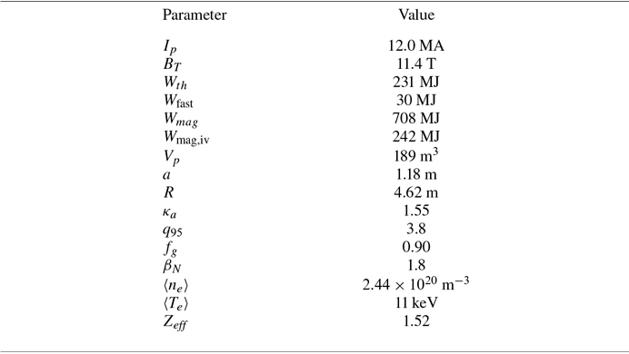


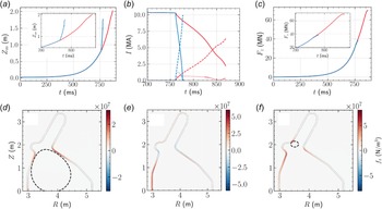


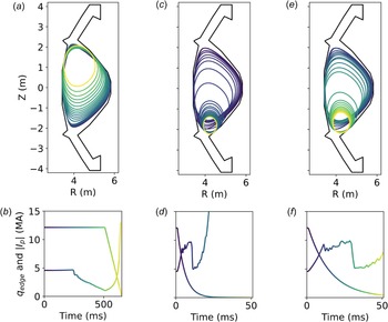

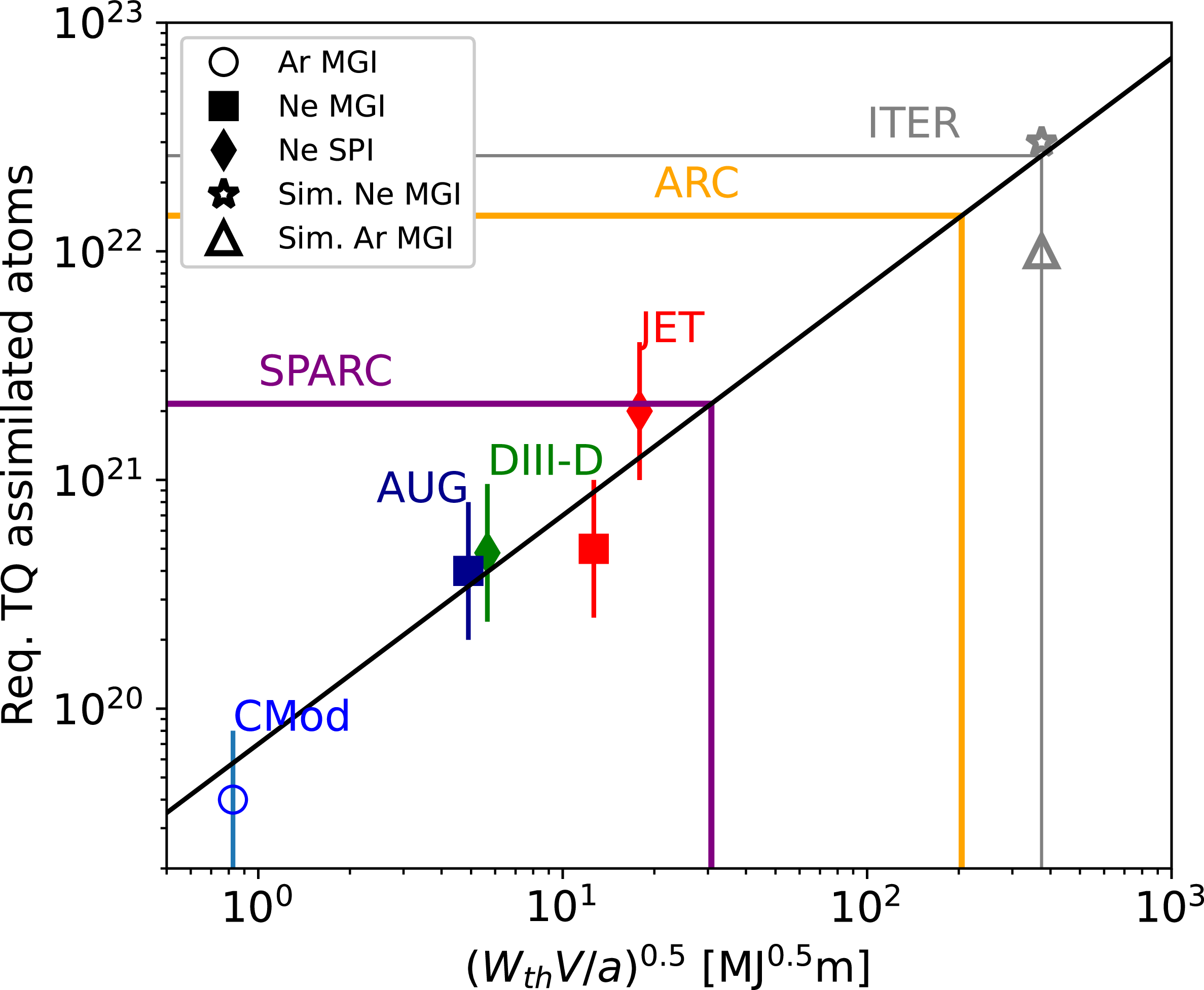


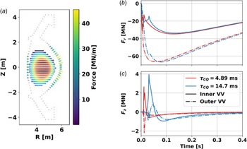


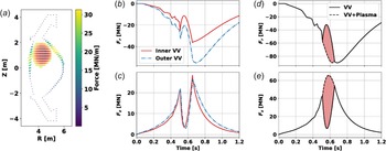


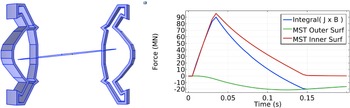


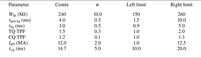





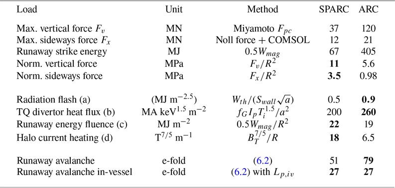

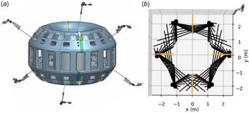
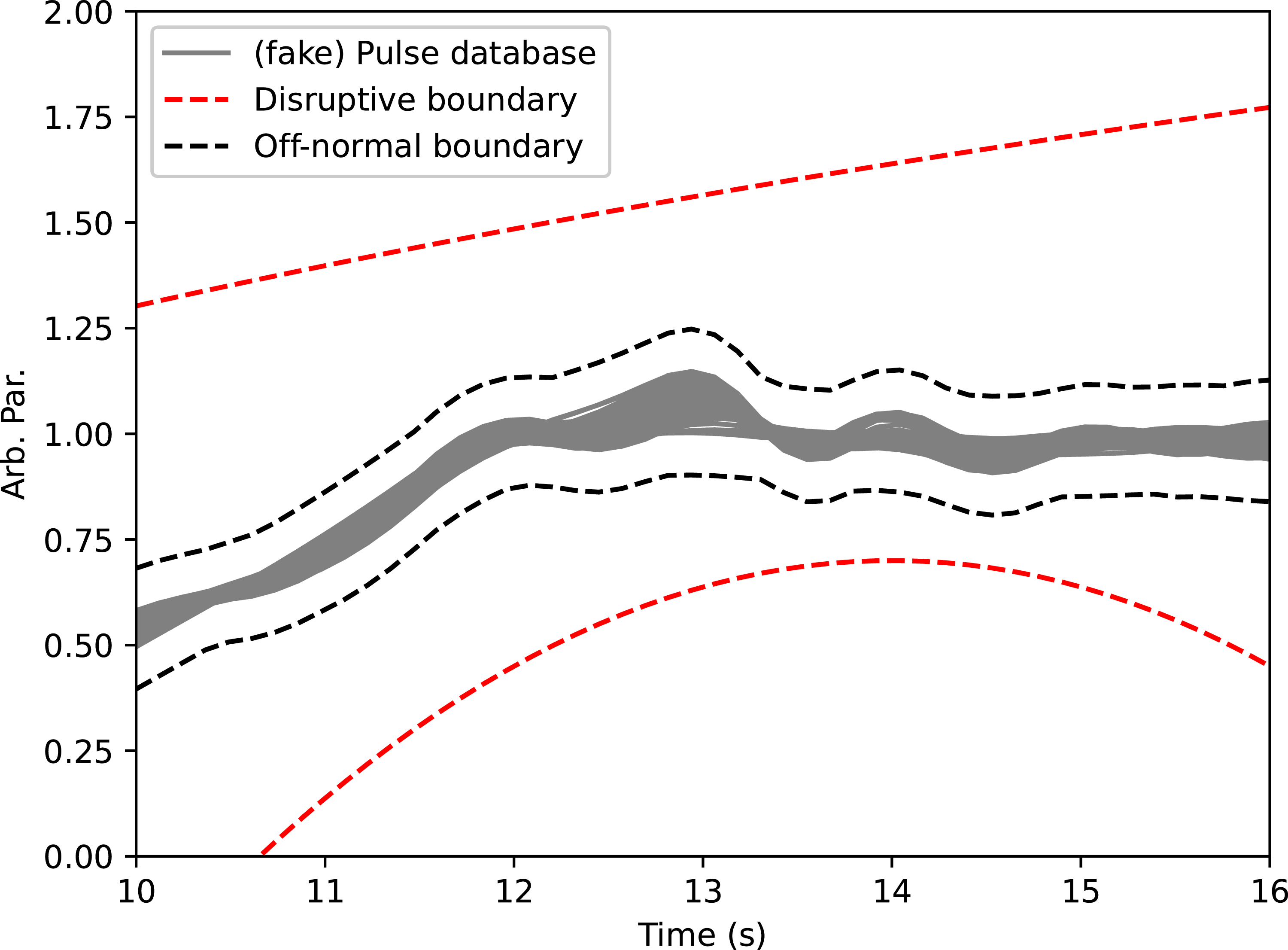


 Open access

